Formulas for Counting the Sizes of Markov Equivalence Classes of Directed Acyclic Graphs

Abstract

The sizes of Markov equivalence classes of directed acyclic graphs play important roles in measuring the uncertainty and complexity in causal learning. A Markov equivalence class can be represented by an essential graph and its undirected subgraphs determine the size of the class. In this paper, we develop a method to derive the formulas for counting the sizes of Markov equivalence classes. We first introduce a new concept of core graph. The size of a Markov equivalence class of interest is a polynomial of the number of vertices given its core graph. Then, we discuss the recursive and explicit formula of the polynomial, and provide an algorithm to derive the size formula via symbolic computation for any given core graph. The proposed size formula derivation sheds light on the relationships between the size of a Markov equivalence class and its representation graph, and makes size counting efficient, even when the essential graphs contain non-sparse undirected subgraphs.

Keywords: Directed acyclic graph; Markov equivalence class; Size formula; Causality

1 Introduction

A Markov Equivalence class contains all statistically equivalent models of directed acyclic graphs (DAG) (Pearl, 2000; Spirtes et al., 2001). In general, observational data is not sufficient to distinguish an underlying DAG from the others in the same Markov equivalence class. The size of a Markov equivalence class is the number of DAGs in the class. It plays an important part in papers to measure the “uncertainty” of causal graphs or to evaluate the “complexity” of a Markov equivalence class in causal learning (He and Geng, 2008; Chickering, 2002). For example, He and Geng (2008) propose several criterions, all of which are defined on the sizes of Markov equivalence classes, to measure the uncertainty of causal graphs for a candidate intervention; choosing interventions by minimizing these criterions makes helpful but expensive interventions more efficient. Maathuis et al. (2009) introduce a method to estimate the average causal effects of the covariates on the response by considering the DAGs in the equivalence class; the size of the class determines the complexity of the estimation.

An essential graph represents a Markov equivalence class and its undirected subgraphs determine the size of the class (Andersson et al., 1997). The size of a small Markov equivalence class can be counted via traversal methods that list all DAGs in the Markov equivalence class (Gillispie and Perlman, 2002). Recently, He et al. (2015) propose a size counting algorithm that calculates the size of a Markov equivalence class via partitioning the class recursively. In general, this method is efficient for Markov equivalence classes represented by sparse essential graphs, but becomes much time-consuming when the essential graphs contain non-sparse undirected subgraphs.

Counting graphs based on formulas is usually elegant and efficient. Robinson (1973, 1977) provide recursive formulas to count DAGs with a given number of vertices. Steinsky (2003) develops recursive formulas to count Markov equivalence classes of size 1. Later, Gillispie (2006) introduces recursive formulas for arbitrary size, based on all configurations of the undirected essential graphs that produce this size. However, there are few formulas available for counting the size of a given Markov equivalence class, except five formulas introduced in He et al. (2015) for Markov equivalence classes represented by five specific types of undirected essential graphs (trees, graphs with up to two missing edges, etc.).

In this paper, we focus on the formulas for counting the size of a Markov equivalence class. We first introduce a new concept of “core graph”, which is an undirected chordal graph without dominating vertices. An undirected essential graph can be represented by its core graph and the number of dominating vertices. The size of the corresponding Markov equivalence class is a polynomial of the number of dominating vertices given its core graph. Then we develop an iterative method to derive the polynomial, and give the explicit polynomials for both several specific types of core graphs and all core graphs with up to five missing edges. Based on symbolic computation, we introduce a size formula derivation algorithm and a formula-based size counting algorithm for general core graphs and Markov equivalence classes, respectively. Our experiments show that the proposed size formula derivation is efficient in general and formula-based algorithm can speedup size counting dramatically for the Markov equivalence classes represented by essential graphs with non-sparse undirected subgraphs.

The rest of the paper is arranged as follows. In Section 2, we give a brief introduction about Markov equivalence class and size counting of Markov equivalence classes. In Section 3, we propose a method to derive the size formulas and to count the sizes of Markov equivalence classes based on these formulas. In Section 4, we study the size formulas and formula-based size counting of Markov equivalence classes experimentally. We conclude in Section 5 and finally present all proofs in the Appendix.

2 Markov Equivalence Class and Size Counting

A graph ${\cal G}$ consists of a vertex set $V$ and an edge set $E$. A graph is directed (undirected) if all of its edges are directed (undirected). A sequence of edges that connect distinct vertices in $V$, say $\{v_{1},\cdots,v_{k}\}$, is called a path from $v_{1}$ to $v_{k}$ if either $v_{i}\to v_{i+1}$ or $v_{i}-v_{i+1}$ is in $E$ for $i=1,\cdots,k-1$. A path is partially directed if at least one edge in the path is directed. A path is directed (undirected) if all edges are directed (undirected). A cycle is a path from a vertex to itself.

A directed acyclic graph (DAG) $\cal D$ is a directed graph without any directed cycle. Let $V$ be the vertex set of $\cal D$ and $\tau$ be a subset of $V$. The induced subgraph ${\cal D}_{\tau}$ of $\cal D$ over $\tau$, is defined to be the graph whose vertex set is $\tau$ and whose edge set contains all of those edges of $\cal D$ with two end points in $\tau$. A v-structure is a three-vertex induced subgraph of $\cal D$ like $v_{1}\rightarrow v_{2}\leftarrow v_{3}$. A graph is called a chain graph if it contains no partially directed cycles. The isolated undirected subgraphs of the chain graph after removing all directed edges are the chain components of the chain graph. A chord of a cycle is an edge that joins two nonadjacent vertices in the cycle. An undirected graph is chordal if every cycle with four or more vertices has a chord.

A graphical model is a probabilistic model for which a DAG denotes the conditional independencies between random variables. A Markov equivalence class is a set of DAGs that encode the same set of conditional independencies. Let the skeleton of an arbitrary graph $\cal G$ be the undirected graph with the same vertices and edges as $\cal G$, regardless of their directions. Verma and Pearl (1990) prove that two DAGs are Markov equivalent if and only if they have the same skeleton and the same v-structures. Moreover, Andersson et al. (1997) show that a Markov equivalence class can be represented uniquely by an essential graph, denoted by ${\cal C}$, which has the same skeleton as ${\cal D}$, and an edge is directed in ${\cal C}$ if and only if it has the same orientation in every equivalent DAG of $\cal D$. An essential graph is a chain graph and each of its chain components is an undirected and connected chordal graph (UCCG for short).

Let Size$({\cal C})$ denote the size of the Markov equivalence class represented by $\cal C$ (size of $\cal C$ for short). Clearly, $\mbox{Size}({\cal C})=1$ if $\cal C$ is a DAG; otherwise $\cal C$ may contain at least one chain component, denoted by ${\cal C}_{\tau_{1}},\ldots,{\cal C}_{\tau_{k}}$. We can calculate the size of $\cal C$ by counting the DAGs in Markov equivalence classes represented by its chain components using the following equation (He and Geng, 2008; Gillispie and Perlman, 2002):

$$\mbox{Size}({\cal C})=\prod_{i=1}^{k}\mbox{Size}({\cal C}_{\tau_{i}}).$$ (1)

Since each chain component is an undirected and connected chordal graph, to obtain the size of a Markov equivalence class, it is sufficient to compute the size of Markov equivalence classes represented by these UCCGs according to Equation (1).

Let ${\cal U}$ be a UCCG, $\tau$ be the vertex set of $\cal U$ and $\cal D$ be a DAG in the equivalence class represented by $\cal U$. A vertex $v$ is a root of $\cal D$ if all directed edges adjacent to $v$ are out of $v$, and $\cal D$ is $v$-rooted if $v$ is a root of $\cal D$. A $v$-rooted sub-class of $\cal U$ is the set of all $v$-rooted DAGs in the Markov equivalence class represented by $\cal U$. A $v$-rooted essential graph of ${\cal U}$, denoted by ${\cal U}^{(v)}$, is a graph that has the same skeleton as ${\cal U}$, and an edge is directed in ${\cal U}^{(v)}$ if and only if it has the same orientation in every $v$-rooted DAG of $\cal U$. He et al. (2015) show that a $v$-rooted sub-class of $\cal U$ can be represented uniquely by a $v$-rooted essential graph and a Markov equivalence class can be partitioned into sub-classes represented by its rooted essential graphs.

Lemma 1

Let ${\cal U}$ be a UCCG over $\tau=\{{v_{i}}\}_{i=1,\cdots,p}$, ${\cal U}^{(v_{i})}$ be $v_{i}$-rooted essential graph, and $f({\cal U}^{(v_{i})})$ be the size of $v_{i}$-rooted sub-class represented by ${\cal U}^{(v_{i})}$. We have $\emph{Size}({\cal U}^{(v_{i})})\geq 1$ for any $i=1,\cdots,p$, and

$$\emph{Size}({\cal U})=\sum_{i=1}^{p}\emph{Size}({\cal U}^{(v_{i})}).$$ (2)

For any $i\in\{1,\cdots,p\}$, the undirected subgraphs of ${\cal U}^{(v_{i})}$ in Lemma 1 are UCCGs, so we can calculate $\mbox{Size}({\cal U}^{(v_{i})})$ in Equation (2) using Equation (1). As a result, using Equation (1) and Equation (2), He et al. (2015) propose to calculate the size of a Markov equivalence class by partitioning it recursively into rooted sub-classes until the sizes of all these sub-classes can be completely determined by the numbers of vertices and edges. However, when the UCCGs contain non-sparse subgraphs, this method might be much time-consuming.

In the next section, we will show that the size of the Markov equivalence class represented by a UCCG depends on a subgraph of the UCCG, and introduce a size formula derivation algorithm and a formula-based counting algorithm, which can greatly accelerate size counting of Markov equivalence classes with non-sparse undirected subgraphs.

3 Formulas for sizes of Markov equivalence classes

In this section, we introduce the concept of core graph that determines the size formula of a Markov equivalence class in Section 3.1. Then, we discuss the recursive and explicit formulas for the size of a Markov equivalence class given its core graph in Section 3.2. Finally, in Section 3.3, we provide algorithms to derive size formulas and to count the sizes of Markov equivalence classes based on these formulas.

3.1 Core graph

A vertex is dominating in a UCCG $\cal U$ if it is adjacent to all other vertices in $\cal U$. A dominating vertex pruned subgraph of $\cal U$ is obtained by removing some dominating vertices from $\cal U$. We denote a dominating vertex pruned subgraph of $\cal U$ as ${\cal U}^{m-}$ if it is obtained by removing $m$ dominating vertices from $\cal U$. An extended graph of $H$, denoted by ${H}^{m+}$, is a graph obtained by adding $m$ dominating vertices to $H$.

Definition 2 (Core graph of a UCCG)

The core graph of $\cal U$ is the minimal dominating vertex pruned subgraph of $\cal U$.

Let $m$ be the number of dominating vertices in $\cal U$, $\cal K$ be the core graph of $\cal U$. Clearly, $\cal K$ is the same as ${\cal U}^{m-}$. If $\cal U$ is a completed graph, all vertices in $\cal U$ are dominating, so the core graph of $\cal U$ is a null graph. Let $\cal K$ be an undirected graph over $V$. Clearly, according to Definition 2, the undirected graph $\cal K$ is a core graph of some UCCG if and only if $\cal K$ is an undirected chordal graph without dominating vertices. The complement of $\cal K$, denoted by ${\cal K}^{c}$, is a graph on the same vertices and an edge appears in ${\cal K}^{c}$ if and only if it does not occur in $\cal K$. Proposition 3 presents a property of the complement of a core graph.

Proposition 3 (Complement of core graph)

Let $\cal U$ be a UCCG, $m$ be the number of dominating vertices in $\cal U$, $\cal K$ be the core graph of $\cal U$, ${\cal K}^{c}$ be the complement of $\cal K$. We have that ${\cal K}^{c}$ be a connected graph, and for any two edges in ${\cal K}^{c}$, either they share a common vertex, or they are connected by an edge.

This property helps us to construct a core graph. In Table 1, we list all core graphs and the corresponding complement graphs of the UCCGs with up to three missing edges.

Number ( missing edges)	0	1	2	3
$\cal K$	${\cal K}_{\emptyset}$
${\cal K}^{c}$	${\cal K}_{\emptyset}$

Table 1: Core graphs and their complements when at most three edges are missing, $\cal K$, ${\cal K}^{c}$, and ${\cal K}_{\emptyset}$ denote a core graph, the complement of $\cal K$, and a null graph, respectively.

Let $\cal U$ be a UCCG with $m$ dominating vertices, $\cal K$ be the core graph of $\cal U$. As an extended graph of $\cal K$, $\cal U$ is the same as ${\cal K}^{m+}$ regardless the labels of vertices, so we have $\mbox{Size}({\cal U})=\mbox{Size}({\cal K}^{m+})$. Clearly, the size of the Markov equivalence class represented by a UCCG $\cal U$ is determined by its core graph $\cal K$ and the number of dominating vertices $m$. For an undirected chordal graph $\cal K$ and a nonnegative integer $m$, we define a function $f({\cal K},m)$ as following,

$$f({\cal K},m):=\mbox{Size}({\cal K}^{m+}).$$ (3)

From the definition of the formula $f({\cal K},m)$, we have the following lemma directly.

Lemma 4

Let ${\cal K}$ be an undirected chordal graph, and ${\cal K}^{k+}$ be an extended graph of ${\cal K}$, we have $f({{\cal K}^{k+}},m)=f({\cal K},m+k)$.

Consider the UCCGs with at most two missing edges, as shown in Table 1, there is only one core graph exists, so the sizes of the corresponding Markov equivalence classes are determined given the number of vertices in the UCCGs. When three edges are missing in the UCCGs, there are three core graphs exists, so three sizes are possible given the number of vertices. This explains the results introduced in He et al. (2015) that the size of a Markov equivalence class is determined given the number of vertices ($p$) only when no more than two edges are missing in UCCGs.

The size of $\cal U$ might be very huge; for a UCCG $\cal U$ with $p$ vertices, $\mbox{Size}({\cal U})$ reaches the maximum $p!$ when $\cal U$ is a completed graph. In general, more edges in the UCCG (more denser), more larger the corresponding class and more time-consuming of size counting. Fortunately, a dense UCCG $\cal U$ might has sparse core graph $\cal K$ when many dominating vertices exist. In the next section, given the core graph $\cal K$, we will discuss the formula of $f({\cal K},m)$ that can be used to speedup the enumeration of $\mbox{Size}({\cal U})$.

3.2 Size formulas based on core graphs

In this section, we propose a method to derive the size formula $f({\cal K},m)$ defined in Equation (3). We first introduce a recursive formula of $f({\cal K},m)$ given $\cal K$, then propose a method to derive the explicit size formulas, and finally give the explicit formulas for both several specific types of core graphs and all core graphs with up to five missing edges.

Theorem 5 introduces the main recursive formula for the size of a Markov equivalence class whose representation graph is extended from an undirected chordal graph $\cal K$ as follows.

Theorem 5

Let $\cal K$ be an undirected chordal graph over $V$. For any integer $m\geq 0$, ${\cal K}^{m+}$ is an extended graph of $\cal K$, and $f({\cal K},{m})$ is the size of ${\cal K}^{m+}$ defined in Equation (3). We have $f\left({\cal K},{0}\right)=\emph{Size}({\cal K})$, and for any integer $m>0$,

$$f\left({\cal K},{m}\right)=m\cdot f\left({\cal K},{m-1}\right)+\sum_{v\in V}f\left({\cal K}_{N_{v}},{m}\right)\frac{\emph{Size}\left({\cal K}^{(v)}\right)}{\emph{Size}\left({\cal K}_{N_{v}}\right)},$$ (4)

where ${\cal K}^{(v)}$ is a v-rooted graph of ${\cal K}$ and ${\cal K}_{N_{v}}$ is an induced subgraph on the neighbors of $v$.

Theorem 5 shows that the size function $f({\cal K},{m})$ can be calculated through the term $f({\cal K},{m-1})$ and the terms related to some subgraphs of $\cal K$. Below, we discuss the explicit formula of $f({\cal K},{m})$. First, we have the following corollary.

Corollary 6

Let ${\cal K}$ be an undirected chordal graph. The formula $f({\cal K},{m})$ defined in Equation (3) is a polynomial divisible by $m!$.

Consider the recursive formula in Equation (4), the second term in the right side is crucial to derive the explicit formula of $f({\cal K},{m})$. Define

$$g({\cal K},m):=\frac{1}{m!}\sum_{v\in V}f({\cal K}_{N_{v}},{m})\frac{\mbox{Size}({\cal K}^{(v)})}{\mbox{Size}({\cal K}_{N_{v}})}.$$ (5)

If $\cal K$ is an undirected chordal graph, its induced subgraph ${\cal K}_{N_{v}}$ is also an undirected chordal graph. According to Corollary 6, the formula $f({\cal K}_{N_{v}},{m})$ is a polynomial divisible by $m!$, it follows that the formula $g({\cal K},m)$ defined in Equation (5) is a polynomial of $m$. Let $d$ be the degree of polynomial $g({\cal K},m)$, according to Corollary 6, $g({\cal K},m)$ can be represented by

$$g({\cal K},m)=\sum_{i=1}^{d+1}\gamma_{i}m^{i-1}.$$ (6)

Given the polynomial $g({\cal K},m)$, the following theorem shows the explicit formula of $f({\cal K},{m})$.

Theorem 7

Let ${\cal K}$ be an undirected chordal graph, $\{\gamma_{i},i=1,2,\cdots,d+1\}$ be the coefficients of the polynomial $g({\cal K},m)$ defined in Equation (6), and let $a_{ij}=(-1)^{j-i}{j\choose{i-1}}$ for any $i\leq j$. We have, for any $m\geq 0$,

$${f({\cal K},{m})}=\left(\beta_{0}+\sum_{i=1}^{d+1}\beta_{i}m^{i}\right){m!},$$ (7)

where $\beta_{0}=\mbox{Size}({\cal K})$, $\beta_{d+1}={\gamma_{d+1}}/{a_{d+1,d+1}}$, and $\beta_{i}=({{\gamma_{i}-\sum_{j=i+1}^{d+1}a_{i,j}\beta_{j}}})/{{a_{i,i}}},$ for any integer $i\in[1,d]$.

According to Theorem 7, to obtain the explicit formula of $f({\cal K},m)$ for an undirected chordal graph $\cal K$, we just need to calculate the size $\mbox{Size}(\cal K)$, and the polynomial $g({\cal K},m)$ defined in Equation (6). The algorithms for general core graphs $\cal K$ will be introduced in Section 3.3. Below, we discuss the formulas for some specific types of undirected chordal graphs.

When an undirected chordal graph contains some isolated vertices, these vertices can be removed and the corresponding size formula can be obtained as follows.

Corollary 8 (Isolated vertices)

The graph $\cal K$ is composed of an undirected chordal graph ${\cal K}_{1}$ and $j$ isolated vertices. We have

$$f({\cal K},{m})=f({\cal K}_{1},{m})+j\cdot\mbox{Size}({\cal K}_{1})\cdot mm!.$$ (8)

Especially, when ${\cal K}_{1}$ is a null graph, we have $f({\cal K},{m})=(jm+1)m!$.

A tree is a connected graph without cycle, and a tree plus graph is generated by adding one more edge to a tree. We give four explicit size formulas for four specific types of undirected chordal graphs in Corollary 9.

Corollary 9

Let $\cal K$ be an undirected chordal with $p$ vertices.

1. If ${\cal K}$ is a null graph, we have $f({{\cal K}},{m})=m!$.

2. If $\cal K$ is a tree, we have $f({\cal K},{m})=[(p-1)m^{2}+(2p-1)m+p]m!$.

3. If $\cal K$ is a tree plus, we have $f({\cal K},{m})=[m^{3}+2pm^{2}+(4p-1)m+2p]m!$.

4. If $\cal K$ is composed of isolated edges, we have $f({\cal K},{m})=2^{p/2-1}(pm^{2}/2+3pm/2+2)m!$.

id	$(n^{\prime},p)$	$\cal K$	$f({\cal K},{m})/m!$	id	$(n^{\prime},p)$	$\cal K$	$f({\cal K},{m})/m!$
1	(1, 2)		$2m+1$	9	(4,5)		$24m+(m+4)\cdots(m+1)$
2	(2,3)		$m^{2}+5m+2$	10	(5,4)		$m^{2}+7m+2$
3	(3,3)		$3m+1$	11	(5,5)		$2m^{3}+11m^{2}+29m+10$
4	(3,4)		$3m^{2}+7m+4$	12	(5,5)		$m^{3}+10m^{2}+19m+10$
5	(3,4)		$m^{3}+6m^{2}+17m+6$	13	(5,5)		$m^{3}+10m^{2}+19m+10$
6	(4,4)		$4m^{2}+12m+4$	14	(5,6)		$m^{4}+14m^{3}+55m^{2}+82m+40$
7	(4,4)		$2m^{2}+8m+3$	15	(5,6)		$(m+1)(2m+3)(m^{2}+7m+16)$
8	(4,5)		$(m+1)(m+4)(2m+3)$	16	(5,6)		$120m+(m+5)\cdots(m+1)$

Table 2: The explicit formulas for all core graphs with up to five missing edges, $n^{\prime},p$ are the number of missing edges and the number of vertices in the core graph $\cal K$, respectively.

By Corollary 8, corollary 9 and Theorem 7, we can obtain the size formula $f({\cal K},m)$ given an undirected chordal graph $\cal K$. He et al. (2015) give two explicit size formulas for essential graphs with one or two missing edges; here we do the same for core graphs with at most five missing edges. In Table 2, we list all core graphs with up to five missing edges, together with their corresponding size formulas. We give an example to demonstrate the derivation of these formulas. Consider the last (with id 16) core graph in Table 2, $\cal K$ is composed of a completed graph with five vertices (${\cal K}_{1}$) and one isolated vertex. We have Size$({\cal K}_{1})=120$ and $f({\cal K}_{1},m)=(m+5)!$ from Lemma 4, it follows $f({\cal K},m)/m!=[(m+5)!+120mm!]/m!=120m+(m+5)\cdots(m+1)$ by Corollary 8.

Given an undirected connected chordal graph $\cal U$, when its core graph $\cal K$ is small, we can calculate $g({\cal K},m)$ directly following its definition in Equation (5), and then obtain the explicit formula of $f({\cal K},{m})$ according to Theorem 7. However, when the core graph is large, the derivation of $g({\cal K},m)$ becomes more complicated. In the next section, we will provide an algorithm to derive the explicit formulas of $f({\cal K},{m})$ for a general core graph $\cal K$.

3.3 Algorithms

In this section, we introduce two main algorithms. The algorithm SizeF$({{\cal K}})$ in Algorithm 1 gives the explicit formula of $f({{\cal K}},{m})$ for an undirected chordal graph $\cal K$. The algorithm Size$({\cal C})$ in Algorithm 2 counts the size of the Markov equivalence class represented by an essential graph $\cal C$. Both Algorithm 1 and Algorithm 2 call each other recursively.

1

Input: ${\cal K}$, an undirected chordal graph;

Output: $f({{\cal K}},{m})$, a polynomial of $m$.

2

3Let type be the type of ${\cal K}$ and $p$ be the number of vertices in ${\cal K}$;

4 switch type do

5      case null graph do return $m!$;

6        ;

7       case tree do return $[(p-1)m^{2}+(2n-1)m+p]m!$;

8        ;

9       case tree-plus do return $(m^{3}+2pm^{2}+(4p-1)m+2p)m!$;

10        ;

11       case isolated-edge graph do return $2^{p/2-1}(pm^{2}/2+3pm/2+2)m!$;

12       

13

14Let $w$ be the number of dominating vertices in ${\cal K}$; remove these vertices from $\cal K$;

15

16if $w>0$ then

17      

18      ${h}(m)\leftarrow$ SizeF$({\cal K})$;

19       return h(m+w)

20

21Let $k$ be the number of isolated vertices in ${\cal K}$; remove these vertices from ${\cal K}$;

22

23if $k>0$ then

24       return ${\emph{SizeF}}({{\cal K}})+\emph{Size}({\cal K})kmm!$, (see Size(${\cal K}$) in Algorithm 2);

25      

26

27return SizeGF(${\cal K}$), (see SizeGF(${\cal K}$) in Algorithm 3);

28

Algorithm 1 SizeF$({{\cal K}})$

1

Input: $\cal C$, an essential graph;

Output: the size of Markov equivalence classes represented by ${\cal C}$.

2 Let ${\cal C}_{1},\cdots,{\cal C}_{J}$ be all of chain components of $\cal U$; for any integer $0\leq J\leq J$, $m_{j}$ is the number of dominating vertices in ${\cal C}_{j}$ and ${\cal K}_{j}$ the core graph of ${\cal C}_{j}$;

3 for $j\leftarrow 1$ to $J$ do

4       $f_{j}(m)\leftarrow$ SizeF(${\cal K}_{i}$) ;

return $\prod_{j=1}^{J}f_{j}(m_{j})$.

Algorithm 2 Size$({\cal C})$

In Algorithm 1, we first give the explicit formula of $f({\cal K},m)$ when $\cal K$ is null, tree, tree-plus or isolated-edge graph according to Proportion 9. Otherwise, when the undirected chordal graph $\cal K$ contains dominating vertices or isolated vertices, we simplify the formula derivation according to Lemma 4 or Corollary 8, respectively. Finally, for a general undirected chordal graph $\cal K$, we derive the explicit formula of $f({\cal K},{m})$ by the algorithm called SizeGF(${\cal K}$) in Algorithm 3.

The algorithm SizeGF(${\cal K}$) in Algorithm 3 first calculates the polynomial $g({\cal K},m)$ defined in Equation (6) and then derives the explicit polynomial $f({\cal K},m)$ according to Theorem 7. Suppose that the undirected chordal graph $\cal K$ contains $J$ isolated connected subgraphs, we calculate the polynomial $g({\cal K},m)$ in the first part of Algorithm 3 (line 1 to 4) according to Corollary 10 as follows.

Corollary 10

Let $\cal K$ be an undirected chordal graph with $J$ isolated connected subgraphs, denoted by ${\cal K}_{1},\cdots,{\cal K}_{J}$ respectively, $V({\cal K}_{j})$ be the set of vertices in ${\cal}K_{j}$, and $g({\cal K},m)$ is the polynomial defined in Equation (6). We have

$$g({\cal K},m)=\sum_{j=1}^{J}\frac{\mbox{Size}({\cal K})}{\mbox{Size}({\cal K}_{j})}\sum_{v\in V({\cal K}_{j})}\frac{f({\cal K}_{j,N_{v}},{m})}{m!}\frac{\mbox{Size}({\cal K}_{j}^{(v)})}{\mbox{Size}({\cal K}_{j,N_{v}})},$$ (9)

where ${\cal K}_{j}^{(v)}$ is the $v$-rooted essential graph of ${\cal K}_{j}$, and ${\cal K}_{j,N_{v}}$ is the induced subgraph of ${\cal K}_{j}$ on the neighbours of $v$.

1

Input: ${\cal K}$, an undirected chordal graph;

Output: $f({{\cal K}},{m})$, a polynomial of $m$.

2

3Let ${{\cal K}}_{1},\cdots,{{\cal K}}_{J}$ be $J$ UCCGs in ${\cal K}$, $V({\cal K}_{j})$ be the vertex set of ${\cal}K_{j}$;

4 Set $S_{{\cal K}_{j}}^{(v)}\leftarrow{\mbox{Size}({\cal K}_{j}^{(v)})}$ for any integer $j\in[1,J]$ and any $v\in V({{\cal K}}_{j})$;

5 $S_{{\cal K}_{j}}\leftarrow\sum_{v\in V({\cal K}_{j})}{\mbox{Size}({\cal K}_{j}^{(v)})}$, $S_{\cal K}\leftarrow\prod_{j=1}^{J}S_{{\cal K}_{j}}$;

6

7$g(m)\leftarrow\sum_{j=1}^{J}\frac{S_{\cal K}}{S_{{\cal K}_{j}}}\sum_{v\in V({\cal K}_{j})}\frac{\mbox{SizeF}({\cal K}_{j,N_{v}})}{m!}\frac{S_{{\cal K}_{j}}^{(v)}}{\mbox{Size}({\cal K}_{j,N_{v}})}$ and denote it as $\sum_{i=1}^{d+1}\gamma_{i}m^{i-1}$;

8 Set $\beta_{0}\leftarrow S_{\cal K}$; $\beta_{d+1}\leftarrow{\gamma_{d+1}}/{a_{d+1,d+1}}$ and $a_{ij}\leftarrow(-1)^{j-i}{j\choose{i-1}}$ for $i\leq j\leq d+1$;

9 for $i\leftarrow d$ to $1$ do

10      $\beta_{i}\leftarrow\frac{\gamma_{i}-\sum_{j=i+1}^{d+1}a_{i,j}\beta_{j}}{a_{i,i}}$;

return $\sum_{i=0}^{d+1}\beta_{i}m^{i}$m!.

Algorithm 3 SizeGF$({{\cal K}})$

In Algorithm 3, we need to calculate $\mbox{Size}({\cal K}_{j}^{(v)})$ for some $j$ and $v$, which are the sizes of Markov equivalence classes represented by rooted essential graphs. He et al. (2015) propose an algorithm called ChainCom to construct the rooted essential graph and all of its chain components for a UCCG and a root vertex. We give ChainCom in Algorithm 4 in Appendix for the completion of the paper.

In Algorithm 2, we first find the core graphs of the chain components of the essential graph $\cal C$, then calculate the size of the corresponding Markov equivalence class by using the formulas obtained from Algorithm 1. When some subgraphs of these chain components contain dominating vertices, formula-based size counting will display its advantages; this will be studied experimentally in the next section.

4 Experimental Results

In this section, we introduce the implementation of the formula derivation and formula-based counting algorithms, and conduct experiments to evaluate the formula-based size counting algorithm proposed in Section 3. All experiments are run on a linux server at Intel 2.0GHz. These experiments display that the proposed alorithms greatly speed up the size counting, especially when the corresponding UCCGs contain dense subgraphs.

4.1 A Python package for size formula derivation

We developed a Python package named countMEC to derive the size formulas and to count the sizes of Markov equivalence classes based on these formulas. The symbolic computation in countMEC depends on the python package sympy. The following example demonstrates the usage of the package countMEC.

1. from countMEC import *
2. G=ran_conn_chordal_graph(15,95)
3. K=core_graph(G)
4. F=SizeF([K])
5. S=Size(G)

In this example, we first import the package countMEC, and randomly generate a UCCG $G$ with 15 vertices and 95 edges. The graph $G$ is shown in the left of Figure 1. Then, we get the core graph of $G$, denoted by $K$, which is shown in the right of Figure 1. The graph $G$ contains $7$ dominating vertices and the core graph $K$ just contains 8 vertices and 17 edges. In the fourth line, we call SizeF($\cdot$) (Algorithm 1); it outputs the following size formula: $F(m)=\left(m^{3}+16m^{2}+77m+108\right)(m+2)!$. In the last line, we call Size($\cdot$) (Algorithm 2) and get $S=643749120$, which is the size of $G$. It’s easy to check that $S=F(7)$. In this example, it takes 0.5 second to count size using the proposed formula-based algorithm, while 440 seconds are taken with the method introduced in He et al. (2015); we will compare the time complexities of two methods thoroughly in the next section.

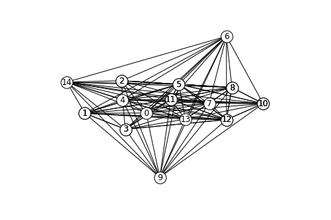
$$G$$

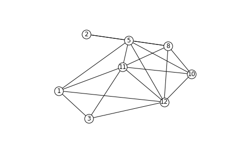
$$K$$

Figure 1: A UCCG $G$ with 15 vertices and 95 edges and its core graph $K$.

4.2 Formula-based size counting

In this section, we experimentally compare the time complexity of our proposed counting algorithms to the benchmark algorithm introduced in He et al. (2015). Let ${\mathbb{U}}_{p}^{n}$ be the set of Markov equivalence classes with $p$ vertices and $n$ edges. We obtain random choral graphs from ${\mathbb{U}}_{p}^{n}$ following He et al. (2015). First, we construct a tree by connecting two vertices (one is sampled from the connected vertices and the other from the isolated vertices) sequentially until all $p$ vertices are connected. Then, we randomly insert an edge such that the resulting graph is chordal, repeatedly until the number of edges reaches $n$. Repeating this procedure $N$ times, we obtain $N$ samples from ${\mathbb{U}}_{p}^{j}$ for each integer $j(\leq n)$.

We first consider the UCCGs in ${\mathbb{U}}_{p}^{n}$ with $p\leq 12$ for each integer $n\in[p+2,p(p-1)/2-3]$. Because the results have the similar patterns for different $p$, we just report the experiments for $p=12$ in this paper. Based on the $10^{5}$ samples from ${\mathbb{U}}_{12}^{n}$ for each integer $n\in[14,63]$, we plot the mean, the minimum, the median, and the maximum of the counting time used by the benchmark algorithm (blue dashed lines) and by the proposed Algorithm 2 (red solid lines) in four panels of Figure 2, respectively. In each panel of Figure 2, the main window displays all results ($n\in[14,63]$) of both algorithms, the two upper sub-windows display the results of both algorithms for $n\in[14,39]$ and $n\in[40,50]$, respectively, and the lower sub-window displays the results of Algorithm 2 again with a proper size-coordinate.

We see that the counting time (mean, minimum, median, and maximum) of the benchmark algorithm is increasing in the number of edges ($n$); size counting based on benchmark algorithm becomes much time-consuming when the graphs are dense. Meanwhile, the time used by Algorithm 2, increases first, and then decreases with the number of edges. Figure 2 shows that size counting based on Algorithm 2 keeps efficient for both sparse and dense graphs.

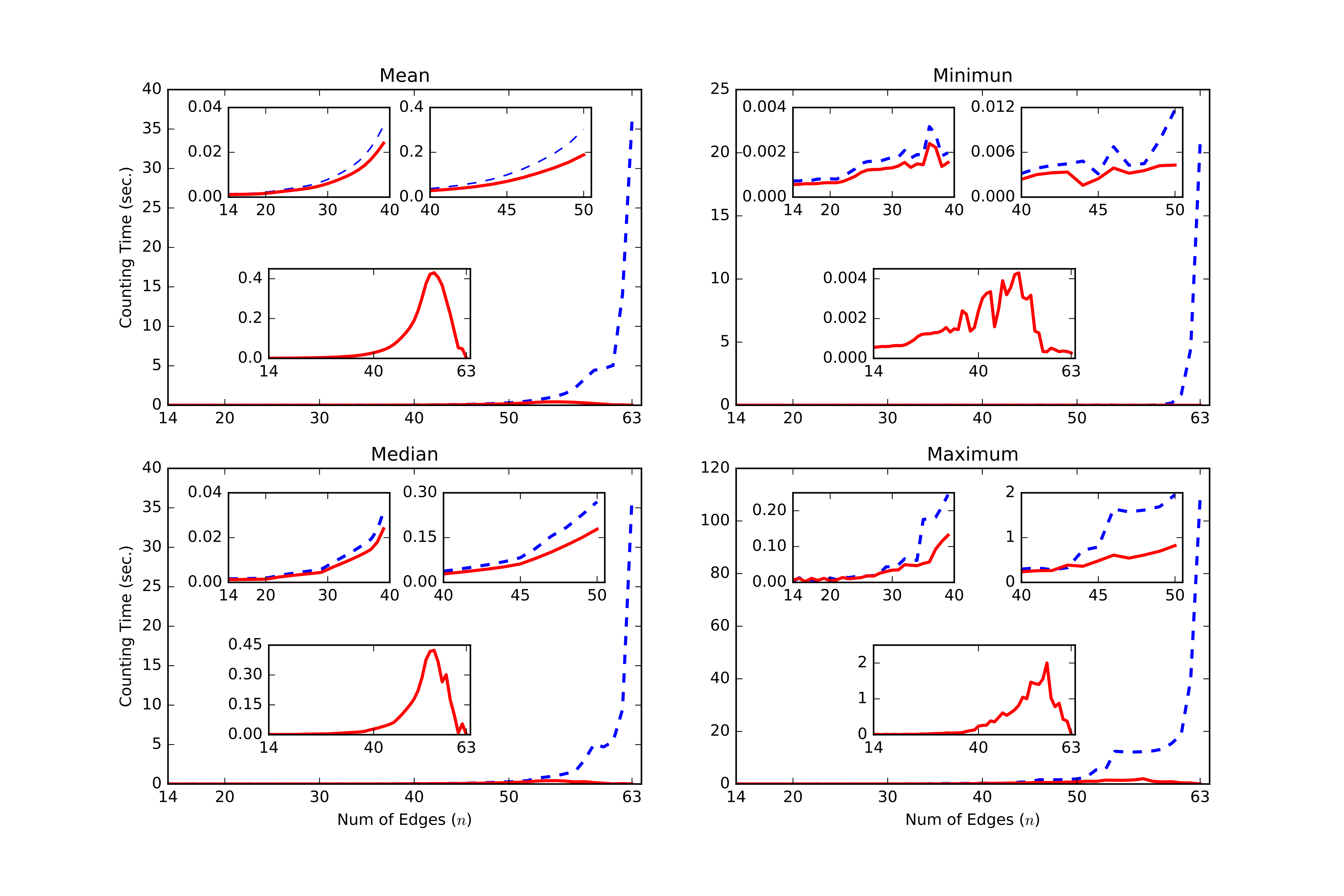
Figure 2: The mean, the minimum, the median and the maximum of counting time of Markov equivalence classes with 12 vertices and $n$ edges.

We also study the sets ${\mathbb{U}}_{p}^{n}$ that contain UCCGs with tens of vertices under sparsity constraints. The number of vertices $p$ is set to $20,50$, and $100$, and the number of edges $n$ is set to $rp$ where $r$ is the ratio of $n$ to $p$. For each $p$, we consider three ratios: 3, 4 and 5. The graphs in ${\mathbb{U}}_{p}^{rp}$ are sparse since $r\leq 5$. For each pair of $(p,r)$, $10^{5}$ UCCGs are generated randomly and then sorted in ascending order according to the counting time used by benchmark algorithm. The ordered $10^{5}$ UCCGs are divided into four subsets. The subset $S_{1}$ contains the first 500 UCCGs, $S_{2}$ contains the next 49500 UCCGs, $S_{3}$ contains the next 49500 UCCGs after $S_{2}$, and $S_{4}$ contains the last 500 UCCGs. For each subset, we report the average of counting time and the average of their ratios in Table 3 for the benchmark algorithm ($T_{1}$) and the proposed algorithm 2 ($T_{2}$). We see that on average, (1) the proposed Algorithm 2 is faster than the benchmark algorithm in all cases, (2) the more edges the UCCGs have ($r$ from $3$ to $5$), or the more time benchmark algorithm used (subset from $S_{1}$ to $S_{4}$), the smaller $T_{2}/T_{1}$, that is, the higher speedup Algorithm 2 achieved. For example, consider the subsets $S_{4}$ and $r=5$, the average counting time is shorten rapidly for all $p\in\{20,50,100\}$, the average of ratios $T_{2}/T_{1}$ are also reduced to nearly 0.02.

$p$		Subset		$r$
				$3$				$4$				$5$
				$T_{1}$	$T_{2}$	$T_{2}/T_{1}$		$T_{1}$	$T_{2}$	$T_{2}/T_{1}$		$T_{1}$	$T_{2}$	$T_{2}/T_{1}$
20		$S_{1}$		0.01	0.01	0.76		0.02	0.02	0.76		0.02	0.02	0.75
		$S_{2}$		0.03	0.03	0.77		0.17	0.13	0.74		1.47	0.96	0.67
		$S_{3}$		0.10	0.07	0.74		1.03	0.52	0.63		21.73	4.38	0.38
		$S_{4}$		0.68	0.32	0.55		21.14	2.23	0.17		954.22	10.92	0.02
50		$S_{1}$		0.07	0.05	0.79		0.19	0.15	0.79		0.74	0.56	0.76
		$S_{2}$		0.18	0.14	0.77		0.77	0.55	0.73		5.82	3.21	0.59
		$S_{3}$		0.55	0.40	0.74		5.18	2.39	0.59		113.22	17.46	0.34
		$S_{4}$		5.62	2.10	0.41		238.98	18.80	0.15		17598.39	128.65	0.02
100		$S_{1}$		0.26	0.21	0.80		0.73	0.58	0.80		3.18	2.27	0.71
		$S_{2}$		0.78	0.60	0.77		2.92	2.05	0.71		21.86	10.90	0.53
		$S_{3}$		2.25	1.63	0.74		19.96	9.04	0.56		429.61	55.63	0.27
		$S_{4}$		21.14	7.81	0.43		897.18	59.59	0.10		59093.25	516.44	0.02

Table 3: The average of counting time ($T_{1}$ for benchmark algorithm and $T_{2}$ for Algrithm 2) and ratios ($T_{2}/T_{1}$) for UCCGs with $p$ vertices and $pr$ edges in different subsets.

We have to point out that the choral graphs generated in our experiments might not be uniformly distributed in the space of chordal graphs and that the results in Figure 2 and Table 3 are not accurate estimations of expectations of the corresponding statistics.

5 Conclusion and discussion

In this paper, we propose a method to derive the size formulas of Markov equivalence classes and to count the sizes based on these formulas. A core graph of an undirected connected chordal graph is introduced and the size formula derivation based on the core graph is proposed. We discuss both recursive and explicit forms of the size formulas and give algorithm to derive these formulas. Comparing to the benchmark counting algorithm, the proposed algorithm can generate more size formulas efficiently, and by these formulas, size counting is accelerated dramatically when the essential graph contains non-sparse undirected subgraphs.

Acknowledgments

This work was supported partially by NSFC (11671020, 11101008, 71271211).

A Algorithm ChainCom(${\cal U},v$)

For the completion of the paper, we give the algorithm ChainCom$({\cal U},v)$ in Algorithm 4, which is introduced in He et al. (2015), to construct the rooted essential graph ${\cal U}^{(v)}$ and all of its chain components.

1

Input: $\cal U$, a UCCG; $v$, a vertex of $\cal U$.

Output: $v-$rooted essential graph of $\cal U$ and all of its chain components.

2

3Set $A=\{v\}$, $B=\tau\setminus v$, ${\mathcal{G}}={\cal U}$ and ${\cal O}=\emptyset$

4while $B$ is not empty do

5       Set ${T}=\{w:w\mbox{ in }{B}\mbox{ and adjacent to $A$}\}$ ;

6      

7      Orient all edges between $A$ and $T$ as $c\to t$ in $\cal G$, where $c\in A,t\in T$;

8      

9      repeat

10             for each edge $y-z$ in the vertex-induced subgraph ${\cal G}_{T}$ do

11                   if $x\to y-z$ in $\mathcal{G}$ and $x$ and $z$ are not adjacent in $\mathcal{G}$ then

12                        Orient $y-z$ to $y\to z$ in $\mathcal{G}$

13                  

14            

15      until  no more undirected edges in ${\cal G}_{T}$ can be oriented ;

16      Set ${A}=T$ and ${B}={B}\setminus{T}$;

17       Append all isolated undirected graphs in ${\cal G}_{T}$ to $\cal O$;

18      

19

return $\cal G$ and ${\cal O}$

Algorithm 4 ChainCom$({\cal U},v)$

B Proofs of Results

In this section, we provide the proofs of the main results of our paper.

Proof of Proposition 3

Let $v_{i_{1}}-v_{j_{1}}$ and $v_{i_{2}}-v_{j_{2}}$ be two edges in ${\cal K}^{c}$. If neither they share a common vertex, nor they are connected by an edge, we have that $v_{i_{1}},v_{j_{1}},v_{i_{2}},v_{j_{2}}$ are four distinct vertices and there is no edge between $v_{i_{1}},v_{j_{1}}$ and $v_{i_{2}},v_{j_{2}}$. Since that $\bar{\cal K}$ is the complement of $\cal K$, we have that the four edges, $v_{i_{1}}-v_{i_{2}}$, $v_{i_{2}}-v_{j_{1}}$, $v_{j_{1}}-v_{j_{2}}$, and $v_{j_{2}}-v_{i_{1}}$ appear in $\cal K$, and meanwhile, the two edges $v_{i_{1}}-v_{j_{1}}$ and $v_{i_{2}}-v_{j_{2}}$ do not occur in $\cal K$. This implies that no chord exists in the cycle $v_{i_{1}}-v_{i_{2}}-v_{j_{1}}-v_{j_{2}}-v_{i_{1}}$ in $\cal K$. It is a contradiction because $\cal K$ is a chordal graph.

Since no dominating vertices appear in $\cal K$, for any vertex $v$ in $\cal K$, there exists another vertex in $\cal K$ such that it is not adjacent to $v$. Consequently, there is no isolated vertex in ${\cal K}^{c}$. Following the proof in the last paragraph, there are no two edges that occur separatively in two isolated subgraphs of $\cal K$. As a result, ${\cal K}^{c}$ is a connected graph. $\blacksquare$

Before proving Theorem 5, we give the following lemma.

Lemma 11

Let $\cal U$ be an undirected chordal graph over $V$ and ${\cal U}^{(v)}$ be the v-rooted graph of $\cal U$. We have that the subgraph of ${\cal U}^{(v)}$ on the neighbors of $v$, denoted by ${\cal U}_{N_{v}}^{(v)}$, is undirected.

Proof  We can get ${\cal U}^{(v)}$ using Algorithm 4. Consider any edge, denoted by $v_{i}-v_{j}$, in ${\cal U}_{N_{v}}$, $v,v_{i}$ and $v_{j}$ form a triangle. According to Algorithm 4, $v_{i}-v_{j}$ can not be oriented to a directed edge since $v\to v_{i}-v_{j}$ is not a induced subgraph of $\cal U$. Therefore, we have that ${\cal U}_{N_{v}}^{(v)}$ is undirected.  

Proof of Theorem 5

Denote the vertices of ${\cal K}$ as $V=\{v_{1},\cdots,v_{p}\}$, and the $m$ extended vertices in ${\cal K}^{m+}$ as $V^{\prime}=\{v_{p+1},\cdots,v_{p+m}\}$. From Lemma 1, we have

$$f\left({{\cal K},{m}}\right)=\sum_{v\in V}\mbox{Size}\left(({{\cal K}^{m+}})^{(v)}\right)+\sum_{v\in V^{\prime}}\mbox{Size}\left(({{\cal K}^{m+}})^{(v)}\right).$$ (10)

For any $v\in V^{\prime}$, since $v$ is adjacent to all other vertices in ${{\cal K}^{m+}}$, from Lemma 11, we have $\mbox{Size}\left(({{\cal K}^{m+}})^{(v)}\right)=f\left({{\cal K},{m-1}}\right)$ and

$$\sum_{v\in V^{\prime}}\mbox{Size}\left(({{\cal K}^{m+}})^{(v)}\right)=m\cdot f\left({{\cal K},{m-1}}\right).$$ (11)

For any $v\in V$, the neighbor set of $v$ in ${\cal K}^{(m+)}$ is $N_{v}\cup V^{\prime}$, from Lemma 11, ${({\cal K}_{N_{v}})}^{m+}$ is a chain component of $({{\cal K}^{m+}})^{(v)}$ when $m>0$. According to Algorithm 4 and Lemma 11, the directions of edges among $v$, $N_{v}$ and $V^{\prime}$ and the other vertices in $({{\cal K}^{m+}})^{(v)}$ are displayed in Figure 3. All edges are directed from $N_{v}\cup V^{\prime}$ to $V-N_{v}\cup\{v\}$ in $({{\cal K}^{m+}})^{(v)}$. We have

$$\mbox{Size}\left(({{\cal K}^{m+}})^{(v)}\right)=\mbox{Size}\left(\left(({{\cal K}^{m+}})^{(v)}\right)_{N_{v}\cup V^{\prime}}\right)\mbox{Size}\left(\left(({{\cal K}^{m+}})^{(v)}\right)_{V-N_{v}\cup\{v\}}\right)$$

First, according to Lemma 11, we can get that $\left(({{\cal K}^{m+}})^{(v)}\right)_{N_{v}\cup V^{\prime}}$ is the same as ${({\cal K}_{N_{v}})}^{m+}$, thus, $\mbox{Size}\left(\left(({{\cal K}^{m+}})^{(v)}\right)_{N_{v}\cup V^{\prime}}\right)=f\left({{\cal K}_{N_{v}}},{m}\right)$ holds. Then, consider the undirected edges in $\left(({{\cal K}^{m+}})^{(v)}\right)_{V-N_{v}\cup\{v\}}$, according to Algorithm 4, because all vertices in $V^{\prime}$ are parents of vertices in $V-N_{v}\cup\{v\}$, we have that $\left(({{\cal K}^{m+}})^{(v)}\right)_{V-N_{v}\cup\{v\}}$ has the same chain components as $\left({\cal K}^{(v)}\right)_{V-N_{v}\cup\{v\}}$. As a result, $\mbox{Size}\left(\left(({{\cal K}^{m+}})^{(v)}\right)_{V-N_{v}\cup\{v\}}\right)=\mbox{Size}\left(\left({\cal K}^{(v)}\right)_{V-N_{v}\cup\{v\}}\right)$. Moreover, according to Equation (1), we have $\mbox{Size}\left(\left({\cal K}^{(v)}\right)_{V-N_{v}\cup\{v\}}\right)=\frac{\mbox{Size}({\cal K}^{(v)})}{\mbox{Size}({\cal K}_{N_{v}})}$. Consequently, we have

$$f\left(({{\cal K}^{m+}})^{(v)}\right)=f({{\cal K}_{N_{v}}},{m})\frac{\mbox{Size}({\cal K}^{(v)})}{\mbox{Size}({\cal K}_{N_{v}})}.$$ (12)

Theorem 5 holds directly from Equation (10), Equation (11) and Equation (12).

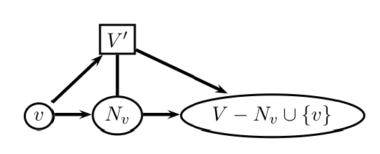
Figure 3: The directions of edges among $v$, $N_{v}$ and $V^{\prime}$ and the other vertices in $({{\cal K}^{m+}})^{(v)}$, where $v\to N_{v}$ represents that each edge between $v$ and $N_{v}$ is directed from $v$ to the vertex in $N_{v}$, and $V^{\prime}-N_{v}$ represents that all edges between $V^{\prime}$ and $N_{v}$ are undirected.

$\blacksquare$

Proof of Corollary 6

For any undirected chordal graph $\cal K$, from Theorem 5, we have

$$f\left({\cal K},{m}\right)=m\cdot f\left({\cal K},{m-1}\right)+\sum_{v\in V}f\left({\cal K}_{N_{v}},{m}\right)h({\cal K},v)$$ (13)

where $V$ is the set of vertices in $\cal K$, $h({\cal K},v)$ is an integer function of $\cal K$ and $v$. Consider $f(\cdot,\cdot)$ terms in the right side of Equation (13), we can calculate them by using Equation (13) again as follows.

$$f\left({\cal K},{m-1}\right)=(m-1)\cdot f\left({\cal K},{m-2}\right)+\sum_{v\in V}f\left({\cal K}_{N_{v}},{m-1}\right)h({\cal K},v)$$ (14)

and

$$f\left({\cal K}_{N_{v}},{m}\right)=m\cdot f\left({{\cal K}_{N_{v}}},{m-1}\right)+\sum_{v^{\prime}\in N_{v}}f\left({{\cal K}}_{N^{\prime}_{v^{\prime}}},{m}\right)h({\cal K}_{N_{v}},v),$$ (15)

where $N^{\prime}_{v^{\prime}}$ is the neighbor set of $v^{\prime}$ in ${\cal K}_{N_{v}}$. Replacing $f\left({\cal K},m-1\right)$ and $f\left({\cal K}_{N_{v}},{m}\right)$ in Equation (13) by the corresponding terms in Equation (14) and Equation (15), we can find that $f\left({\cal K},{m}\right)$ is the sum of the following three types of terms,

1. $m(m-1)f({\cal K},{m-2})$,

2. $mf({{\cal K}_{N_{v}}},{m-1})h({\cal K},v)$, for any $v\in V({\cal K})$, and

3. $f({{\cal K}}_{N^{\prime}_{v^{\prime}}},{m})h({\cal K}_{N_{v}},v)$, where $N^{\prime}_{v^{\prime}}$ is the neighbor set of $v^{\prime}$ in ${\cal K}_{N_{v}}$, for any $v^{\prime},v$ such that $v^{\prime}\in N_{v}$.

Notice that for any $v,v^{\prime}$, we have $N^{\prime}_{v^{\prime}}\subset N_{v}\subset V$, so the graphs in above three types of terms are smaller than that in Equation (13). By this way, using Equation (13) repeatedly, we can calculate $f({\cal K},{m})$ by smaller graphs. Finally, $f({\cal K},{m})$ can be calculated only by $f({\cal K},{0})$ and $f(({\cal K}_{\emptyset}),{k})$ for $k\leq m$. As a result, $f({\cal K},{m})$ is the sum of some polynomials of $m$ and each term of the polynomials contains either $m!f({\cal K},{0})$ or $\frac{m!}{k!}f(({\cal K}_{\emptyset}),{k})$ for $k\leq m$. Because ${\cal K}_{\emptyset}$ is null graph, $f(({\cal K}_{\emptyset}),{k})=k!$, we have that $f({\cal K},{m})$ is a polynomial divisible by $m!$. $\blacksquare$

Proof of Theorem 7

We just need to show that Formula (7) is the solution of Equation (4). First, when $m=0$, we have $f({\cal K},{m})=\beta_{0}=\mbox{Size}({\cal K})$. Theorem 7 holds if the following equation holds,

$$\left(\beta_{0}+\sum_{i=1}^{d+1}\beta_{i}m^{i}\right){m!}=m\left(\beta_{0}+\sum_{i=1}^{d+1}\beta_{i}(m-1)^{i}\right){(m-1)!}+\sum_{i=1}^{d+1}\gamma_{i}m^{i-1}m!.$$

Equivalently,

$$\sum_{i=1}^{d+1}\beta_{i}m^{i}-\sum_{i=1}^{d+1}\beta_{i}(m-1)^{i}=\sum_{i=1}^{d+1}\gamma_{i}m^{i-1}$$ (16)

Consider the left side of Equation (16),

$$\begin{array}[]{rl}\sum_{i=1}^{d+1}\beta_{i}\left[m^{i}-(m-1)^{i}\right]=&\sum_{i=1}^{d+1}\beta_{i}\left[\sum_{j=0}^{i-1}(-1)^{i-(j+1)}{i\choose j}m^{j}\right]\\ =&\sum_{j=0}^{d}\sum_{i=j+1}^{d+1}\left[(-1)^{i-(j+1)}{i\choose j}\beta_{i}m^{j}\right]\\ =&\sum_{k=1}^{d+1}\left[\sum_{i=k}^{d+1}(-1)^{i-k}{i\choose k-1}\beta_{i}\right]m^{k-1}\end{array}$$

If Equation (16) holds for any $m>0$, we have that $\sum_{i=k}^{d+1}(-1)^{i-k}{i\choose k-1}\beta_{i}=\gamma_{k}$ holds for any $k=1,\cdots,d+1$. Let

$$A=\left(\begin{array}[]{cccc}a_{11}&a_{12}&\cdots&a_{1,d+1}\\ 0&a_{22}&\cdots&a_{2,d+1}\\ \vdots&\vdots&\ddots&\vdots\\ 0&0&\cdots&a_{d+1,d+1}\\ \end{array}\right)=\left(\begin{array}[]{cccc}{1\choose 0}&-{2\choose 0}&\cdots&(-1)^{d}{d+1\choose 0}\\ 0&2\choose 1&\cdots&(-1)^{d-1}{d+1\choose 1}\\ \vdots&\vdots&\ddots&\vdots\\ 0&0&\cdots&{d+1\choose d}\\ \end{array}\right)$$

and $\beta=(\beta_{1},\cdots,\beta_{d+1})^{T}$, and $\gamma=(\gamma_{1},\cdots,\gamma_{d+1})^{T}$. We have

$$A\beta=\gamma.$$

It is easy to verify that $\beta$ in Theorem 7 is the solution of $A\beta=\gamma$. $\blacksquare$

Proof of Corollary 8

Let $v_{1},\cdots,v_{j}$ be the $j$ isolated vertices, $v^{\prime}_{1},\cdots,v^{\prime}_{m}$ be the m extended vertices. $V({\cal K}_{1})$ be the vertices in ${\cal K}_{1}$, $V({\cal K})$ be the vertices in ${\cal K}$. Clearly, we have $V({\cal K})=V({\cal K}_{1})\cup\{v_{1},\cdots,v_{j}\}$

Because $\cal K$ is composed of ${\cal K}_{1}$ and $j$ isolated vertices, Equation (8) holds when $m=0$ since $\mbox{Size}({\cal K})=\mbox{Size}(({\cal K}_{1}))$. Consider the case $m=1$. From Theorem 5, we have

$$f\left({\cal K},{m}\right)=m\cdot f\left({\cal K},{m-1}\right)+\sum_{v\in V({\cal K})}f\left({\cal K}_{N_{v}},{m}\right)\frac{\mbox{Size}\left({\cal K}^{(v)}\right)}{\mbox{Size}\left({\cal K}_{N_{v}}\right)}.$$ (17)

Since $m-1=0$, we have $f({\cal K},{m-1})=\mbox{Size}({\cal K})=\mbox{Size}({\cal K}_{1})$, and $m\cdot f\left({\cal K},{m-1}\right)=m\cdot f({\cal K}_{1})$. Moreover, for any $v\in V({\cal K}_{1})$, $\mbox{Size}({\cal K}^{(v)})=\mbox{Size}(({\cal K}_{1})^{(v)})$ and ${\cal K}_{N_{v}}=({\cal K}_{1})_{N_{v}}$ hold. For any $v\in\{v_{1},\cdots,v_{j}\}$, $\mbox{Size}({\cal K}^{(v)})=\mbox{Size}({\cal K}_{1})$ and ${\cal K}_{N_{v}}$ is a null graph; it follows $f({\cal K}_{N_{v}},m)=m!$ and $\mbox{Size}({\cal K}_{N_{v}})=1$. From Equation (17), we have that

$$\begin{array}[]{rl}f\left({\cal K},{m}\right)&=m\cdot\mbox{Size}\left({\cal K}_{1}\right)+\sum_{v\in V({\cal K}_{1})}f\left({({\cal K}_{1})}_{N_{v}},{m}\right)\frac{\mbox{Size}\left({\cal K}_{1}^{(v)}\right)}{\mbox{Size}\left(({{\cal K}_{1}})_{N_{v}}\right)}+\mbox{Size}({\cal K}_{1})jm!\\ &=f({\cal K}_{1},{m})+\mbox{Size}({\cal K}_{1})jm!=f({\cal K}_{1},{1})+\mbox{Size}({\cal K}_{1})j\end{array}$$

We have Equation (8) holds for $m=1$. Suppose that Equation (8) holds for $m=k-1$, consider $m=k$, from Equation (17), we have

$$f\left({\cal K},{k}\right)=k\cdot f\left({\cal K},{k-1}\right)+\sum_{v\in V({\cal K}_{1})}f\left({({\cal K}_{1})}_{N_{v}},{k}\right)\frac{\mbox{Size}\left({\cal K}_{1}^{(v)}\right)}{\mbox{Size}\left(({{\cal K}_{1}})_{N_{v}}\right)}+\mbox{Size}({\cal K}_{1})jk!$$ (18)

Since Equation (8) holds for $m=k-1$, we have

$$f\left({\cal K},{k-1}\right)=f\left({\cal K}_{1},{k-1}\right)+j(k-1)\mbox{Size}({\cal K}_{1})(k-1)!.$$ (19)

From Theorem 5, we can get

$$f\left({\cal K}_{1},{k}\right)=kf\left({\cal K}_{1},{k-1}\right)+\sum_{v\in V({\cal K}_{1})}f\left({({\cal K}_{1})}_{N_{v}},{k}\right)\frac{\mbox{Size}\left({\cal K}_{1}^{(v)}\right)}{\mbox{Size}\left(({{\cal K}_{1}})_{N_{v}}\right)}.$$ (20)

From Equation (18), (19), and (20), we have

$$\begin{array}[]{rl}f\left({\cal K},{k}\right)=&f\left({\cal K}_{1},{k}\right)+j(k-1)\mbox{Size}({\cal K}_{1})k!+\mbox{Size}({\cal K}_{1})jk!\\ =&f\left({\cal K}_{1},{k}\right)+\mbox{Size}({\cal K}_{1})jkk!.\end{array}$$

As a result, Equation (8) holds for any integer $m\geq 0.$ $\blacksquare$

Proof of Corollary 9

The proof of (1)

When $\cal K$ is null graph, ${\cal K}^{m+}$ is a completed graph with $m$ vertices, the result (1) holds obviously.

The proof of (2)

Let $d_{1},d_{2},d_{3},\cdots,d_{p}$ be degrees of vertices $v_{1},\cdots,v_{p}$ in $\cal K$, we have $\sum_{i=1}^{p}d_{i}=2(p-1)$. Consider $g({\cal K},m)$ defined in Equation (5),

$$g({\cal K},m)=\sum_{i=1}^{p}\frac{f({\cal K}_{N_{v_{i}}},{m})}{m!}\frac{\mbox{Size}({\cal K}^{(v_{i})})}{\mbox{Size}({\cal K}_{N_{v_{i}}})}.$$

Since $\cal K$ is a tree, we have that ${\cal K}_{N_{v_{i}}}$ is composed of $d_{i}$ isolated vertices, so $\frac{f({\cal K}_{N_{v}},{m})}{m!}=1+d_{i}m$. We also have ${f({\cal K}^{(v_{i})})=1}$ and ${f({\cal K}_{N_{v_{i}}})}=1$ if $\cal K$ is a tree. Consequently,

$$g({\cal K},m)=\sum_{i=1}^{p}(1+d_{i}m)=p+2(p-1)m$$

The result (2) holds according to Theorem 7.

The proof of (3)

Consider a tree plus graph, if it is chordal, the added edge must be in a triangle, otherwise, the tree plus graph is not chordal. Let $d_{1},d_{2},d_{3},\cdots,d_{p}$ be degrees of vertices $v_{1},\cdots,v_{p}$ in $\cal K$ and $d_{1},d_{2},d_{3}$ are the degrees of the three vertices in the triangle, we have $\sum_{i=1}^{p}d_{i}=2p$. Moreover,considering the induced subgraph of $\cal K$ over $N_{v_{i}}$, we have that ${\cal K}_{N_{v_{i}}}$ is composed of an edge and $d_{i}-2$ isolated vertices for $i=1,2,3$, and ${\cal K}_{N_{v_{i}}}$ just contains $d_{i}$ isolated vertices for $i=4,5,\cdots,p$. Following Corollary 8, we can calculate $g({\cal K},m)$ as following

$$\begin{array}[]{rl}g({\cal K},m)=&\frac{1}{m!}\left[2(d_{1}+d_{2}+d_{3}-6)mm!+3(m+2)!+2\sum_{i\neq 1,2,3}(d_{i}mm!+m!)\right]\\ =&3m^{2}+4pm-3m+2p\end{array}$$

The result (3) holds according to Theorem 7.

The proof of (4)

Consider a vertex $v$ in $\cal K$, we have that $({\cal K}^{m+})^{(v)}$ contains $p/2$ chain components, in which one is a completed graph with $m+1$ vertices, and the others are one-edge graphs. We can calculate $g({\cal K},m)$ defined in Equation (6) as following

$$g({\cal K},m)=2^{p/2}pm/2+2^{p/2}p/2.$$

As a result, the result (4) holds according to Theorem 7. $\blacksquare$

Proof of Corollary 10

According to the definition of $g({\cal K},m)$ in Equation (5)

$$g({\cal K},m)=\sum_{j=1}^{J}\sum_{v\in V({\cal K}_{j})}\frac{f({\cal K}_{N_{v}},{m})}{m!}\frac{\mbox{Size}({\cal K}^{(v)})}{\mbox{Size}({\cal K}_{N_{v}})}.$$

Because $\cal K$ is composed of ${\cal K}_{1},\cdots,{\cal K}_{J}$ that are $J$ isolated connected graphs, we have that ${\cal K}_{N_{v}}={\cal K}_{j,N_{v}}$, and $\mbox{Size}({\cal K}^{(v)})=\mbox{Size}({\cal K}_{j}^{(v)})\prod_{l\neq j}\mbox{Size}({\cal K}_{l})$ $=\mbox{Size}({\cal K}_{j}^{(v)})\frac{\mbox{Size}({\cal K})}{\mbox{Size}({\cal K}_{j})}$. Consequently, Corollary 10 holds. $\blacksquare$

References

- Andersson et al. (1997) S. A. Andersson, D. Madigan, and M. D. Perlman. A characterization of Markov equivalence classes for acyclic digraphs. The Annals of Statistics, 25(2):505–541, 1997.
- Chickering (2002) D. M. Chickering. Learning equivalence classes of Bayesian-network structures. The Journal of Machine Learning Research, 2:445–498, 2002.
- Gillispie (2006) S. B. Gillispie. Formulas for counting acyclic digraph Markov equivalence classes. Journal of Statistical Planning and Inference, 136(4):1410–1432, 2006.
- Gillispie and Perlman (2002) S.B. Gillispie and M.D. Perlman. The size distribution for Markov equivalence classes of acyclic digraph models. Artificial Intelligence, 141(1-2):137–155, 2002.
- He and Geng (2008) Yangbo He and Zhi Geng. Active learning of causal networks with intervention experiments and optimal designs. Journal of Machine Learning Research, 9:2523–2547, 2008.
- He et al. (2015) Yangbo He, Jinzhu Jia, and Bin Yu. Counting and exploring sizes of markov equivalence classes of directed acyclic graphs. Journal of Machine Learning Research, 16:2589–2609, 2015.
- Maathuis et al. (2009) M. H. Maathuis, M. Kalisch, and P. Bühlmann. Estimating high-dimensional intervention effects from observational data. The Annals of Statistics, 37(6A):3133–3164, 2009. ISSN 0090-5364.
- Pearl (2000) J. Pearl. Causality: Models, Reasoning, and Inference. Cambridge Univ Pr, 2000.
- Robinson (1973) R. Robinson. Counting labeled acyclic digraphs. New Directions in the Theory of Graphs, pages 239–273, 1973.
- Robinson (1977) R. Robinson. Counting unlabeled acyclic digraphs. In Combinatorial mathematics V, pages 28–43. Springer, 1977.
- Spirtes et al. (2001) P. Spirtes, C.N. Glymour, and R. Scheines. Causation, Prediction, and Search. The MIT Press, 2001.
- Steinsky (2003) B. Steinsky. Enumeration of labelled chain graphs and labelled essential directed acyclic graphs. Discrete mathematics, 270(1-3):266–277, 2003.
- Verma and Pearl (1990) T. Verma and J. Pearl. Equivalence and synthesis of causal models. In Proceedings of the Sixth Annual Conference on Uncertainty in Artificial Intelligence, page 270. Elsevier Science Inc., 1990.