The MiMeS survey of magnetism in massive stars: Magnetic analysis of the O-type stars

Abstract

We present the analysis performed on spectropolarimetric data of 97 O-type targets included in the framework of the MiMeS (Magnetism in Massive Stars) Survey. Mean Least-Squares Deconvolved Stokes $I$ and $V$ line profiles were extracted for each observation, from which we measured the radial velocity, rotational and non-rotational broadening velocities, and longitudinal magnetic field $B_{\ell}$. The investigation of the Stokes $I$ profiles led to the discovery of 2 new multi-line spectroscopic systems (HD 46106, HD 204827) and confirmed the presence of a suspected companion in HD 37041. We present a modified strategy of the Least-Squares Deconvolution technique aimed at optimising the detection of magnetic signatures while minimising the detection of spurious signatures in Stokes $V$. Using this analysis, we confirm the detection of a magnetic field in 6 targets previously reported as magnetic by the MiMeS collaboration (HD 108, HD 47129A2, HD 57682, HD 148937, CPD-28 2561, and NGC 1624-2), as well as report the presence of signal in Stokes $V$ in 3 new magnetic candidates (HD 36486, HD 162978, HD 199579). Overall, we find a magnetic incidence rate of $7\pm 3$%, for 108 individual O stars (including all O-type components part of multi-line systems), with a median uncertainty of the $B_{\ell}$ measurements of about 50 G. An inspection of the data reveals no obvious biases affecting the incidence rate or the preference for detecting magnetic signatures in the magnetic stars. Similar to A- and B-type stars, we find no link between the stars’ physical properties (e.g. $T_{\rm eff}$, mass, age) and the presence of a magnetic field. However, the Of?p stars represent a distinct class of magnetic O-type stars.

1 Introduction

Stars of spectral type O are the most massive and luminous stars in the Universe. Due to their intense UV luminosities, dense and powerful stellar winds, and rapid evolution, they exert an impact on the structure, chemical enrichment, and evolution of galaxies that is disproportionate to their small relative numbers.

O-type stars are the evolutionary progenitors of neutron stars and stellar-mass black holes. The rotation of the cores of red supergiants (Maeder & Meynet, 2014a), the characteristics of core collapse supernova explosions (Heger et al., 2005), and the relative numbers, rotational properties and magnetic characteristics of neutron stars (and their exotic component of magnetars) may be sensitive to the magnetic properties of their O-type progenitors. Low-metallicity Oe-type stars have also been associated with the origin of long-soft gamma-ray bursts (e.g. Martayan et al., 2010).

Considering the importance of O stars as drivers of galactic structure and evolution, and the significance of magnetic fields in determining their wind structure (e.g. Shore & Brown, 1990; Babel & Montmerle, 1997; ud-Doula & Owocki, 2002; Townsend & Owocki, 2005), rotation (e.g. ud-Doula et al., 2009; Mikulášek et al., 2008; Townsend, 2010), and evolution (e.g. Meynet et al., 2011; Maeder & Meynet, 2014b), understanding the magnetic characteristics of O stars is of major current interest.

The sample of known magnetic O stars is currently very small - less than a dozen are confidently-identified (Wade & MiMeS Collaboration, 2015). The first magnetic O-type star - the young O dwarf $\theta^{1}$ Ori  C - was discovered to be magnetic by Donati et al. (2002). Measurements of $\theta^{1}$ Ori C by Wade et al. (2006) showed that the field is well-described by a dipole configuration with longitudinal magnetic field strength ($B_{\ell}$) ranging from about $-100$ to 600 G. Modelling of those measurements revealed that the dipolar magnetic field strength is between 1-2 kG and that the magnetic field is oblique to the rotation axis by an angle of $\sim$30-70°. Only one other O star was confidently detected to be magnetic prior to the start of the Magnetism in Massive Stars (MiMeS) survey (the Of?p star HD 191612; Donati et al. 2006).

Within the context of the MiMeS project, HD 191612 was re-observed and found to show $B_{\ell}$ variations from about $-600$ to 100 G. Similarly to $\theta^{1}$ Ori C, the field is well-described by a dipole, with a polar field strength of about 2.5 kG, with a magnetic axis oblique to the rotation axis by about 70°. The O supergiant $\zeta$ Ori A is another O-type star with a highly suspected magnetic field (Bouret et al., 2008). Bouret et al. (2008) observed this star and found marginal evidence for the detection of a Zeeman signature in their observations; however, based on the temporal variability of these signatures, they were able to establish with more confidence that this star hosted the weakest magnetic field of O stars known at this time, with a surface dipolar field strength of about 60 G. The field was also found to be oblique to the rotation axis by about 80°. This result has recently been confirmed within the context of the MiMeS project by Blazère et al. (2015), who identified the $\zeta$ Ori Aa component as the magnetic star with a field strength of $\sim$140 G. Measurements of another Of?p star, HD 148937, were reported to find a detected $B_{\ell}$ ($B_{\ell}/\sigma=3.1$) by Hubrig et al. (2008), but a reanalysis of this observation by Bagnulo et al. (2012) found a slightly reduced $B_{\ell}$ value with a correspondingly reduced detection significance of about 2.9, resulting in only a marginal detection of a magnetic field.

The number of confidently detected magnetic O stars has significantly increased since the start of the MiMeS Project. The MiMeS survey alone was responsible for discovering (or confirming the suspicion of) magnetic fields in 6 O stars: HD 108 (Martins et al., 2010), HD 57682 (Grunhut et al., 2009; Grunhut et al., 2012b), HD 148937 (Wade et al., 2012a), NGC 1624-2 (Wade et al., 2012b), HD 47129A2 (Grunhut et al., 2013), CPD-28 2561 (Wade et al., 2015). Sufficient data exists, and has been reported, for three of these stars (HD 57682, HD 148937, CPD-28 2561) to characterise their magnetic field properties (further details of these observations are discussed in Sect. 4.1). Similar to the previously known magnetic O stars, the magnetic fields in these stars are well described by a mainly centred dipole field, with a polar surface field strength ranging from about 1-3 kG, and a magnetic axis inclined to the rotation axis by about 35-80°.

Other authors (Hubrig et al., 2007a; Hubrig et al., 2008, 2011b, 2012a; Hubrig et al., 2013; Hubrig et al., 2014) have also claimed the detection of a magnetic field in 20 other O-type stars, primarily based on low-resolution FORS data. The validity of several of these and other magnetic claims for different classes of stars based on FORS1 observation were investigated by Bagnulo et al. (2012). In particular, Bagnulo et al., using the same FORS data but a different analysis, could not confirm the detection of a significant number of the reported FORS1 detections. In light of this result, there are serious doubts about the robustness of the reported magnetic claims based on low-resolution data. Despite these many refuted claims, magnetic field detections have been obtained with low-resolution FORS data. Nazé et al. (2012); Nazé et al. (2014) discovered and confirmed the presence of a magnetic field in the cluster star Tr16-22 from a survey consisting of 21 massive stars (including 8 O-type stars). Furthermore, in their study of 50 massive stars (including 28 O-type stars), the BOB collaboration announced the detection of a magnetic field in the O star HD 54879 (Castro et al., 2015; Fossati et al., 2015), using a combination of low-resolution FORS2 and high-resolution HARPSpol observations.

The occurrence of magnetic fields amongst O stars is still debated. Based on the complete sample of known magnetic stars in their study (including non O-type stars), Fossati et al. (2015) found a magnetic incidence rate of $6\pm 4$%, but they only identified one magnetic detection out of 28 O stars, leading to a slightly smaller magnetic incidence fraction of $\sim$4%. Although based on a much smaller sample, the study by Nazé et al. (2012) found one magnetic star out of 8 O stars, leading to a much higher incidence rate of $\sim$13%. These studies, however, deal with small number statistics. Inclusion of any of the previously mentioned studies with refuted claims would also drastically change these statistics.

The MiMeS survey (Wade et al. 2016; hereinafter ‘Paper I’) collected over 4800 high resolution circular polarization spectra of roughly 560 bright stars of spectral types B and O. The aim of the survey is to provide critical missing information about field incidence and statistical field properties for a large sample of hot stars, and to provide a broader physical context for interpretation of the characteristics of known magnetic B and O stars.

In this paper (Paper II), we report the results obtained for all 97 O-type stars (or multiple star systems) obtained within the survey. In Sect. 2, we summarise the target sample, and review the characteristics of the observations. Sect. 3 discusses the Least-Squares Deconvolution analysis of the spectropolarimetric data, including line mask selection and tuning, line profile fitting to derive line broadening and binary parameters, and ultimately the magnetic field diagnosis. In Sect. 4 we report our results, summarising the magnetic detections obtained for the previous MiMeS discoveries, the possible magnetic detections, and the probable spurious detections. In Sect. 5, we discuss tests performed to investigate the reliability of our results, examine the characteristics of the observations and details pertaining to possible trends or subsamples of stars, and compare our results with previous reports of magnetic stars in the literature. Finally, Sect. 6 provides a summary of this study.

2 Sample and observations

As described by Paper I, high-resolution circular polarization (Stokes $V$) spectra of 110 Wolf-Rayet (WR) and O-type targets were collected in the context of the MiMeS Project. Of these targets, 3 magnetic stars ($\theta^{1}$ Ori C, Donati et al. 2002; $\zeta$ Ori A, Bouret et al. 2008; and HD 191612, Donati et al. 2006) were previously known or highly suspected to host a magnetic field and were observed as part of the Targeted Component (TC). The 11 WR stars were previously discussed by de la Chevrotière et al. (2013) and de la Chevrotière et al. (2014) and are not further discussed here with the exception of HD 190918, which also contains a spectroscopic O star companion that is included in this study. In this paper, we focus on the 97 Survey Component (SC) systems that host an O-type star.

A total of 879 Stokes $V$ observations of these 97 targets were obtained with the ESPaDOnS, Narval and HARPSpol echelle spectropolarimeters. As described by Paper I, these instruments acquire high-resolution ($R=65,000$ for ESPaDOnS and Narval, $R=115,000$ for HARPSpol) spectra spanning the optical spectrum (from 370 nm to 1 $\mu$m for ESPaDOnS and Narval, and from 380-690 nm for HARPSpol). A majority (57%) of these spectra were obtained in the context of the MiMeS Large Programs (LPs). The remainder (43%) were collected from the Canada-France-Hawaii Telecsope (CFHT), Télescope Bernard Lyot (TBL) and European Southern Observatory (ESO) archives. While a large number of polarimetric sequences were obtained from the archives, some data for all but 5 targets were acquired from the LPs.

The observed sample of O-type stars is best described as an incomplete, magnitude-limited sample. Approximately 50 bright O stars for which high-resolution IUE spectra exist were identified to be observed during the ESPaDOnS LP, and form the core of the sample. The sample contains a number of stellar subgroups of particular interest for magnetic field investigations, including the peculiar Of?p stars, Oe stars, and weak-wind stars. The Of?p stars were systematically included in the survey (all known Galactic Of?p stars were observed), but other classes of stars (e.g. Oe, weak-wind, etc.) were not systematically targeted, unless specific stars were claimed to be magnetic in the literature. In most cases, stars for which better magnetic sensitivity was likely to be obtained were prioritised. Hence we preferentially observed brighter stars with lower projected rotational velocities.

Fig. 3 of Paper I illustrates the distribution of apparent $V$-band magnitudes of the entire SC sample. Among the O stars, the brightest star of the sample is $V=1.8$, while the faintest has $V=11.8$. The median magnitude of the O star SC sample is about 6.7, which is about 0.5 mag fainter than the combined sample.

Paper I discusses the completeness of the SC sample (illustrated in their Fig. 5), and reported that approximately 7% of all stars with B or O spectral types and brighter than $V=8$ were observed in the survey. However, due to the smaller absolute numbers of bright ($V<8$) O-type stars, the magnitude-limited completeness of the O-type SC sample is much higher: we observed about 43% of all O stars brighter than $V=8$. This is a natural result of the rapid increase of the total number of bright stars toward late B spectral types, combined with our survey focus on the hottest (hence most massive) objects. So even though we observed only one-quarter the number of O stars as B stars, our sampling of the complete population of bright O stars is actually much better

Often, to increase the signal-to-noise ratio (S/N) sufficiently to reach the desired magnetic sensitivity, we acquired multiple successive Stokes $V$ spectra of a target during an observing night. We ultimately co-added the un-normalized spectra obtained on a given night for each star, which led to 432 individual polarized spectra of the 97 targets. For some stars, only one nightly-averaged observation exists, while for others we have several nightly-averaged observations obtained over the course of the project. The analysis for each star was carried out on the co-added nightly averages. Individual polarimetric sequences were also investigated for those stars with high $v\sin i$ or that were previously known to show variations on time-scales shorter than the timespan of the co-added sequence of observations. In each case we found the results were consistent with the nightly averaged spectra.

The S/N of the co-added spectra ranged from about 50 to 6200, with a median of 1005, as computed from the peak S/N per 1.8 km s^-1 pixel of each spectrum, in the 500-650 nm range. The large range in obtained S/N is largely a consequence of varying weather conditions, varying brightness of the targets, and differences due to the adopted exposure times (further discussed below). The 210 ESPaDOnS spectra of 87 individual targets were generally of the highest S/N (1059), but they span a large range in precision (the standard deviation of the sample S/N is 722). The 214 Narval spectra of 23 individual targets were of the next highest precision (median S/N of 980, with a standard deviation of 272). Only a small number (7) of O stars were observed with HARPSpol, yielding a median S/N of 470 for 8 co-added spectra (per $\sim$1.8 km s^-1 velocity bin).

Exposure times for spectra acquired in the context of the LPs were computed using the MiMeS exposure time calculation, which predicts the S/N (and hence exposure time) required to reach a desired “magnetic sensitivity" (see Paper I, Sect. 3.5). Archival observations, on the other hand, adopted their own strategy for determining exposure times based on the requirements of their individual programmes. Despite the different strategies that may have been adopted, the S/N of the archival data (median S/N$\sim$1100, with a standard deviation of 323) is slightly higher than the data obtained within the MiMeS LPs (median S/N$\sim$950, with a standard deviation of 482).

The sample of SC O-type stars and their basic properties are summarised in Table 5 of Paper I.

3 Analysis

3.1 Least-Squares Deconvolution

The Least-Squares Deconvolution technique (LSD; Donati et al., 1997) was applied to all polarimetric spectra to increase the effective S/N in order to detect weak magnetic Zeeman signatures. This multi-line procedure combines information from many metallic and He lines in the spectrum to extract a mean unpolarized intensity profile (Stokes $I$), a mean circularly polarized profile (Stokes $V$), and a mean diagnostic null profile (that characterises spurious signal; e.g. Bagnulo et al. 2009). As input, the procedure requires a “line mask", which contains the predicted central wavelength, the line depth, and the predicted or measured Landé factor. The mean Stokes $I$ profile was constructed from the central line depth-weighted average of all lines included in the line mask, while the mean Stokes $V$ profile was constructed from weighting of the product of the central depth, the central wavelength and the Landé factor of each line in the line mask. Because of this weighting, the LSD procedure is somewhat sensitive to the input line mask (e.g. Donati et al., 1997). In particular, the presence of emission lines and lines that fail the self-similarity assumption of the LSD procedure (i.e. that are not well represented by the average shape of the majority of the other lines), can add destructively to the final line profile. Thus, care must be taken in the construction of the line mask to reduce the effects of these lines, since a relatively small number of lines are available for LSD in the spectra of hot stars (in contrast to the thousands of lines potentially available in the spectra of cool stars, for example).

The primary tool used in this study was the iLSD code of Kochukhov et al. (2010) and an idl front-end developed by one of us (JHG) to extract all profiles on to a velocity grid with a resolution of 1.8 km s^-1. We adopted LSD scaling weights corresponding to a Landé factor of 1.2 and wavelength of 500 nm. To further increase the S/N, we also took advantage of the regularisation capabilities of iLSD by setting the regularisation parameter ($\lambda$) to a value of 0.2 (see Sect. 3.4 for further details).

In order to construct optimal line masks, we first utilised the Vienna Atomic Line Database (VALD2; Piskunov et al., 1995; Kupka et al., 1999) to create the initial “full" line list. The input used appropriate values for their effective temperature ($T_{\rm eff}$) and surface gravity ($\log(g)$), which were based on the spectral type of each star using the corresponding calibration of Martins et al. (2005a), and assumed solar abundances. The full mask included all lines retrieved via an extract stellar request to VALD2 in the range of 370 to 980 nm, with a line-depth cut-off of 1% the continuum. This yielded between 1000 to 2500 lines for each mask, decreasing in number with increasing temperature.

Using an interactive idl code that compares the LSD model (the convolution of the LSD profile with the line mask) with the observed spectrum, we proceeded to develop a “clean" line mask for each observation that excluded all H lines, strong emission lines, lines blended with these lines, and lines blended with strong telluric absorption bands. Finally, we continued to remove all lines that poorly represented the average line profile (e.g. broad He lines) and thus did not satisfy the self-similarity assumption of the LSD procedure.

We next created a “tweaked" mask, whereby we automatically adjusted the depths of the remaining lines to provide the best fit between the LSD model and the observed Stokes $I$ spectrum. This was carried out using the Levenberg-Marquardt, non-linear least-squares algorithm from the mpfit library (Moré, 1978; Markwardt, 2009). The line depths were constrained to have positive values (i.e. absorption lines). The line mask resulting from the successive procedures of cleaning and tweaking was considered the optimal line mask. We found that, with typically only a few hundred lines in the final optimal line mask for each star, the tweaking procedure can greatly improve the quality of fit between the observed spectrum and the LSD model and also improve our ability to detect Zeeman signatures (see Sect. 3.4 for further details). This last step, which essentially assigns empirical depths to each of the remaining lines, also reduces our sensitivity to the choice of input line mask, which may have a slightly different model $T_{\rm eff}$, $\log(g)$ or abundances from the observed star. One of the main results of the tweaking process is to increase the strength of the He lines relative to the metallic lines. The process of cleaning and tweaking greatly reduced the total number of lines in the optimal line mask, to about 200 to 1200 lines. In general, stars with lower effective temperature and narrower line widths had the most lines remaining in their masks; there was no correlation between $\log(g)$ (or luminosity class) and the remaining number of lines from the optimisation procedure. Typically, all elements lighter than Cerium remained in the list, with the majority of the lines comprised of He, C, N, O, Ne, and Fe. All data, LSD profiles, and masks for each star in this study are hosted at a dedicated MiMeS page at the Canadian Astronomy Data Centre (CADC).

While all stars of the same spectral type and luminosity class (independent of other factors such as line width) used the same initial line mask, we optimised the line mask for each star and each observation separately (the same initial cleaned mask was used for each observation, but each observation was tweaked separately). This strategy essentially treats all observations independently (even for the same star), which, in principle, should maximise our ability to detect weak Zeeman signatures from individual observations for stars with multiple observations and a varying spectrum; however, the LSD profiles extracted from a single mask for stars with multiple observations were very similar to the LSD profiles from the individually tailored masks (the usable lines for the LSD procedure did not vary too substantially). Therefore, a single mask per star could have been used and the results presented here would not differ by much.

From each optimal line mask we also used the multi-profile capability of iLSD to simultaneously extract representative mean, unblended profiles of both He and metallic lines. This was accomplished by providing iLSD with two input line masks, one entirely composed of He lines and the other consisting of all other remaining lines in the mask.

In addition to the optimal line mask and its derivatives, we also extracted LSD profiles using the line mask employed by Donati et al. (2006) for Of?p star HD 191612. This line mask contains only 12 lines between 400 and 600 nm, most of which are He lines, in addition to some CNO lines. Despite the relatively few lines employed in this mask, it has proven to yield the most significant Zeeman detections in the discovery of many recent magnetic O-type stars (e.g. Wade et al., 2011; Wade et al., 2012a; Grunhut et al., 2013). From hereon out, this line mask is referred to as the Of?p mask.

The extraction of the final LSD profiles utilised a $\sigma$-clipping procedure (applied to pixel-by-pixel differences between the observed Stokes $I$ spectrum and LSD model). All pixels that differed by more than 50$\sigma$ from the model were rejected and not used in the calculation of the LSD profile. We found this was necessary to reduce the impact of blended telluric features, cosmic rays, echelle ripples, and other general cosmetic issues or spectral contributions that were not of stellar origin.

In a few situations, we encountered extracted LSD Stokes $V$ and diagnostic null $N$ profiles with continuum levels that were systematically offset from zero. This was only observed for observations that were extracted from several co-added high-S/N spectra and the offset appeared to be the same in both Stokes $V$ and $N$. This offset may be due to remnant pseudo-continuum polarization that was not fully subtracted during the libre-esprit reduction process. In order to correct for this effect, we fit a linear function of the form $y=mx+b$ to the LSD diagnostic null profile and subtracted this fit from both the LSD Stokes $V$ and $N$ profiles.

The last step in the calculation of the final LSD profiles was to renormalize each profile to its apparent intensity continuum. A line of the form $y=mx+b$ was fit to the continuum regions (determined interactively) about the Stokes $I$ profiles. We then divided all Stokes profiles ($I$, $V$ and $N$) by this fit.

In addition to using the iLSD code of Kochukhov et al. (2010), we also extracted LSD profiles using the LSD code of Donati et al. (1997) as a consistency check, as it remains the most commonly used code. Unlike the LSD code of Donati et al., iLSD only performs the deconvolution procedure, leaving the user to implement additional operations (some of which have been implemented via our wrapper code, as previously discussed). While the results of the two codes are generally in excellent agreement, the noise characteristics of the LSD profiles can differ in some cases. Furthermore, the use of regularisation, as discussed by Kochukhov et al. 2010, can improve the S/N, which is important in this work as we are searching for weak signals. However, the potentially higher S/N and the difference in the noise characteristics may lead to an increase in spurious signal and the apparent detection of a Zeeman signature (see Sects. 3.3 and 3.4 for further details). As discussed by Donati et al. 1997, several factors can lead to a spurious signal, especially for high S/N observations (e.g. rapid variability of the target, spectrograph drifts, inhomogeneities in CCD pixel sensitivities). We suspect that spurious signals in our sample are most likely caused by small variations in the shape of the line profiles (likely due to stellar variability) from one sub-exposure to the next and small differences in the line profile shape between the two polarization spectra (possibly due to differential optical aberrations or non-uniform fibre illumination). Due to the different treatment of the data by each code, in important specific cases, we also mention the results obtained using the Donati et al. 1997 code in this paper.

3.2 Profile fitting

3.2.1 Single Stars

Each of the final LSD Stokes $I$ profiles were fit following the same procedure as discussed by Neiner et al. (2015). From the fitting procedure, we derived for each profile the radial velocity $v_{r}$, the projected equatorial rotational broadening $v\sin i$, contributions remaining from non-rotational broadening, which we consider as macroturbulent broadening $v_{\rm mac}$, and the line depth. We emphasise that our goal here is to determine reliable $v\sin i$ and total line width measurements, and, as discussed by Simón-Díaz & Herrero (2014), inclusion of $v_{\rm mac}$ is important to avoid over-estimating $v\sin i$. We warn the reader against over-interpreting the $v_{\rm mac}$ results, as the inclusion of He i lines and the LSD technique itself, can introduce additional broadening to the final mean profile (Kochukhov et al., 2010).

Following the strategy adopted by Simón-Díaz & Herrero, each observed profile was compared to a synthetic profile that was computed from the convolution of a rotationally-broadened profile with that of a radial-tangential (RT) macrotubulence broadened profile following the parametrisation of Gray (2005), assuming equal contributions from the radial and tangential component. A linear limb-darkening law was also used to compute the synthetic profiles, with a limb-darkening coefficient of 0.3, which is appropriate for O-type stars (e.g. Claret, 2000). We adopted the RT macroturbulent formalism in our modelling as Simón-Díaz & Herrero have shown a good agreement between their similar profile fitting technique and the more time-consuming (and believed to be more accurate) Fourier technique (Gray, 1981). Furthermore, as the RT broadening does not contribute significantly in the region of the line core, this method should maximise the contribution of rotational broadening to the line profile compared to the more commonly used Gaussian profile for hot OB stars (e.g. Martins et al., 2015). The total line broadening $v_{\rm tot}$ is obtained by adding the $v\sin i$ and $v_{\rm mac}$ in quadrature.

The fitting procedure uses the mpfit library (Moré, 1978; Markwardt, 2009) to find the best fit solution. To further maximise the contribution of rotational broadening, we set the initial guess of $v\sin i$ to the full width half maximum of the profile (identified interactively), and the macroturbulent contribution to one-half of this value. It is certainly possible that the contribution from rotational broadening may be overestimated with this approach and hence our profiles correspond more to “maximal" rotation profiles. Typical uncertainties for the measurements are on the order of 10-20%. Results are presented in Appendix C.

To assess the reliability of our measurements, we compared our results obtained for single stars to those presented by Simón-Díaz & Herrero. In total, 44 stars were found to be in common between both studies, with our $v\sin i$ measurements being about 6% higher on average, with a standard deviation of 20%. We noticed a slight trend between the two different subsets of these measurements. Generally, we achieved a poorer agreement with the results of Simón-Díaz & Herrero for stars with $v\sin i<100$ (on average our results are 16% larger compared Simón-Díaz & Herrero, with a 20% standard deviation), compared to stars with $v\sin i>100$ (our measurements are on average 10% lower, with a 5% standard deviation). While there are some differences between the results of the two studies, the agreement appears consistent within our estimated uncertainties (of 10-20%).

In Fig. 1, we illustrate the achieved quality of fit for two examples: one profile that is dominated by macroturbulent broadening (the magnetic star HD 57682), and one profile with a very high relative contribution of rotational broadening (HD 149757). In the case of HD 57682, the fitted parameters (and the quality of the fit) are in better agreement with values derived using the Fourier technique, and additional constraints derived from the measured rotation period as reported by Grunhut et al. (2012a), than would be the case using a Gaussian profile to represent macroturbulence ($v\sin i$$\sim$13 km s^-1 when using a Gaussian profile vs 8 km s^-1 using the RT formulation; according to Grunhut et al. 2012a, the $v\sin i$ should be on the order of 5 km s^-1).

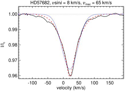
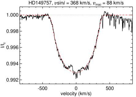
Figure 1: Example LSD profiles illustrating the quality of fit of the profile fitting procedure. The observed LSD profile (solid black) is compared with the best-fitting model profile (dashed red) for one profile dominated by macroturbulence (top panel) and another profile that is dominated by rotational broadening (bottom panel). In the macroturbulence dominated case (top panel), we also illustrate the poorer quality of the fit achieved when using a Gaussian (dotted blue) instead of the radial-tangential formulation for macroturbulence, as adopted in this study.

3.2.2 Spectroscopic multiple systems

For LSD profiles that show signs of multiple spectroscopic components, and for stars that are known spectroscopic binaries, we attempted to simultaneously fit multiple single-star absorption profiles to the observed LSD profile. The individual synthetic fits follow the same description as for the single star case previously discussed, and an overall best fit was determined using mpfit. The simultaneous fitting of multiple profiles for a single observation is a difficult task and the solution is often degenerate. We therefore attempted to constrain each fit based on previously published parameters (e.g. $v\sin i$, radial velocity), whenever possible. The details of the fitting attempts are further discussed in Appendix A. The best fitting parameters are available in Appendix C. These results are simply used to derive the profile fitting parameters (such as radial velocity, line broadening, and line depth), and are not meant to infer any other (physical) parameter of the systems (such as radius/luminosity ratios).

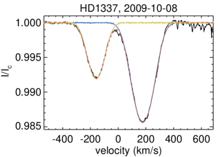
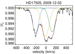
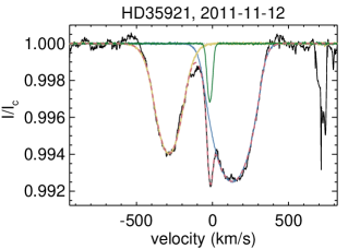
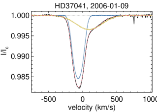
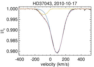
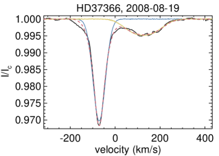
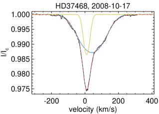
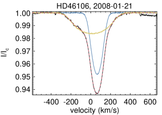
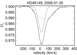
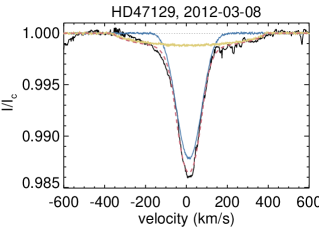
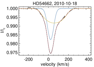
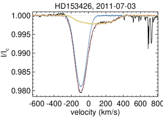
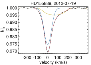
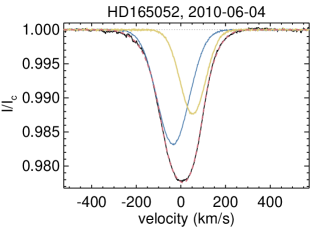
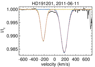
Figure 12: Example unpolarized Stokes $I$ LSD profiles for multi-line spectroscopic binaries for which we were able to fit individual profiles to each component. The solid black line is the observed LSD profile, the solid blue line is the fit to the primary profile, solid yellow line is the fit to the secondary profile, the solid green line is the fit to the tertiary profile (where applicable), and the dashed red line is the combined fit to the observed line profile. The name and observation date have been provided for each profile.

We next constructed semi-empirical ‘disentangled’ profiles for each component in the observed LSD profile by combining the best-fitting Stokes $I$ profile model for each component (random Gaussian noise is also added, in accordance with the S/N of the observation, to preserve the relative noise contribution from each profile for future calculations; however, residual telluric features are the dominant source of “noise" in most profiles, which is not accounted for) with the observed Stokes $V$ and diagnostic $N$ profiles. In the case of non-detections, the use of the fitted profiles better enabled us to determine spectroscopic and magnetic measurements (such as the longitudinal field) for each component separately. This is due to the fact that the velocity limits and a more representative equivalent width measurement could be determined from the separated profiles. In Fig. 2, we provide an example of the achieved quality of fit for an LSD profile showing multiple components. A comparison for all stars is provided in Fig. 12, in Appendix A.

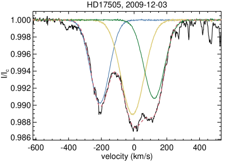
Figure 2: Example LSD profile showing the quality of fit of the multi-profile fitting procedure. The observed LSD profile (solid black) is compared with the best-fitting profiles for each component (indicated by different colours). The thick dashed line shows the co-added profile of the individual components, while the thin horizontal dashed line indicates the continuum level. The additional features in the observed LSD profile reflect telluric blends from some line regions that persist into the final LSD profile.

3.3 Magnetic diagnosis

As discussed in Sect. 3.4 of Paper I, our primary method for establishing the presence of a magnetic field relies on the detection of excess signal in the LSD Stokes $V$ profile, resulting from the longitudinal Zeeman effect, based on the calculation of the False Alarm Probability (FAP), as described by Donati et al. (1992). We quantify the likelihood that a Zeeman signature was detected by measuring the FAP computed from each LSD Stokes $V$ profile, within the confines of the Stokes $I$ line profile (as determined visually Donati et al., 1992). Following Donati et al. (1997), we consider a Zeeman signature to be definitely detected (DD) if the excess signal within the line profile results in a FAP $<10^{-5}$. If the FAP is greater than $10^{-5}$ but less than $10^{-3}$, a signature is considered marginally detected (MD). A FAP greater than $10^{-3}$ is considered a non-detection (ND). In addition to establishing the presence of excess signal within the line profile, we further require that no excess signal is measured outside of the line profile. In the case of some strongly magnetic stars, residual incoherent polarization signal may remain outside of the line profile. However, in such cases the magnetic signal is sufficiently strong that there is no ambiguity concerning its detection; in such cases signatures are usually detectable in individual spectral lines as well. An additional criterion for the evaluation of the reality of the signal is that no excess signal is detected in the null profile. However, radial velocity motions or other line profile variations that occur on timescales of a single polarimetric sequence can result in residual uncancelled signal in the diagnostic null for stars with Zeeman signatures in Stokes $V$. The magnetic signal is typically only slightly affected and sufficiently strong that there is no ambiguity concerning its detection. This problem is common for pulsating stars (e.g. Neiner et al., 2012b). In the event that a FAP leads to a detection within the line profile (FAP $<10^{-5}$), but fails one or more of the other criteria, we consider this to be a marginal detection. Visual inspection of the detected profiles is further carried out to confirm the detection status.

We note that this adopted approach is sensitive to any deviations of the Stokes $V$ profile within the confines of the line profile. In principle, many systematics could result in spurious detections (e.g. rapid variability of the target, spectrograph drifts, inhomogeneities in CCD pixel sensitivities), in addition to random noise. Quality control checks carried out using the large number of null detections (see Sect. 5.1) or analyses performed on the TC (see, for example, Paper I) lead us to understand that the incidence of such artefacts is quite low. Furthermore, examination of the shape, and the coherence of the temporal variation of the Stokes $V$ profile is the best method for verification. Using this guideline as a basis, we consider a detection spurious when the Stokes $V$ profile does not reveal any obvious Zeeman signature and/or the coherence of the temporal variation of this signature is inconsistent with expectations (e.g. the signal is statistically detected in only a few of many observations of similar S/N). A priori, we do not know which stars are magnetic, but, in general, the stars for which we confidently detect magnetic fields show clear evidence of a Zeeman signature in several observations, and, furthermore, the temporal variations of these signatures behave within expectations. The sample of confidently detected magnetic stars have been previously reported by the MiMeS collaboration and consists of: HD 108 (Martins et al., 2010), HD 57682 (Grunhut et al., 2009; Grunhut et al., 2012b), HD 148937 (Wade et al., 2012a), NGC 1624-2 (Wade et al., 2012b), HD 47129A2 (Grunhut et al., 2013), CPD-28 2561 (Wade et al., 2015). For some stars, there is clear evidence for a Zeeman signature in at least one observation, but we lack a sufficient number of observations to confirm this detection. We consider these stars to be potential magnetic candidates.

Since the total velocity width of the line profiles varies substantially from one star to another, we devised a procedure to determine the optimal width of the velocity bin (yielding the most precise magnetic diagnosis) for each individual extracted LSD profile. This was accomplished by maximising the likelihood of detecting a magnetic field by searching for the bin width that provided the lowest FAP. This optimisation requires a delicate balance between increasing the bin width (thereby increasing the S/N per bin) and at the same time decreasing the amplitude of any potential Zeeman signature. To avoid the latter, the maximum allowed bin width was chosen such that the line profile must span a minimum of 20 bins (where possible, limited by the adopted minimum velocity width of 1.8 km s^-1 for the LSD profiles extracted from all instruments - which corresponds to the spectral pixel width for ESPaDOnS and Narval - and the intrinsic width of the line profile). This value was chosen based on our experience of modelling Stokes $V$ profiles resulting from large-scale magnetic fields.

In addition to quantifying the detection of a Zeeman signature using the FAP, we also computed the mean longitudinal magnetic field $B_{\ell}$ using the unbinned profiles from each observation. The longitudinal field was determined using the first-order moment of the Stokes $V$ profile (Rees & Semel, 1979; Mathys, 1989; Donati et al., 1997; Wade et al., 2000):

$$\centering B_{\ell}=-21.4\times 10^{1}1\frac{\int(v-v_{0})V(v)dv}{\lambda zc\int[1-I(v)]dv}.\@add@centering$$ (1)

In this equation, $V(v)$ and $I(v$) represent the continuum normalized Stokes $I$ and $V$ profiles. The mean Landé factor ($z$) and mean wavelength ($\lambda$) correspond to the LSD weights adopted in our analysis (1.2 and 500 nm, respectively), while $c$ is the speed of light. The integration limits are the same as the ones used for the FAP analysis. The uncertainties were computed by propagating the individual uncertainties of each pixel following standard error propagation rules (see Landstreet et al. 2015 Eq. 3 for further details). We also computed similar measurements from the diagnostic null profile $N_{\ell}$ using the same integration limits. Results are available in Appendix C. The $B_{\ell}$ measurements were not used to establish the presence of a magnetic field, as it is possible that a particular magnetic geometry could lead to a net null $B_{\ell}$ measurement, but the velocity-resolved Stokes $V$ profile still shows a clear Zeeman signature due to the combination of the Zeeman and Doppler effects for large-scale fields.

The same analysis described above for single stars was also performed on the disentangled profiles extracted from observations of systems with multiple components. This allowed us to establish magnetic measurements and detection criteria for each component individually; however, this procedure naturally does not account for any possible magnetic contamination in the Stokes $V$ signal from overlapping profiles, i.e. it assumes that the other components are not magnetic. Results are available in the Appendix C.

3.4 Mask comparison

For each observation, we extracted at least 6 LSD profiles using each of the different line masks discussed in Sect. 3.1:

• the original line mask derived from the VALD request

• the ‘cleaned’ version of the VALD line mask

• the optimal ‘cleaned and tweaked’ VALD line mask

• the He-line only ‘cleaned and tweaked’ VALD line mask

• the metal-line only ‘cleaned and tweaked’ VALD line mask

• the Of?p line mask.

For each mask, we examined the binned and unbinned versions of the resulting LSD profiles. When comparing the results for the optimal line mask, we found a noticeable difference in the number of detections among the known magnetic sample. In this case, the optimally binned profiles resulted in about 3 times more detected Zeeman signatures (61) compared to the unbinned profiles (22). This result emphasises the importance of this procedure for such a large sample of stars with different line widths. From this point forward, all discussion of the detection criteria corresponds to the optimally binned profiles, unless otherwise specified.

We also extracted additional LSD profiles with varying values of the regularisation parameter. Regularisation is important, since, as discussed by Kochukhov et al. (2010), it can improve the achievable S/N, which is important in this study as we are searching for weak Zeeman signatures. To assess the performance of the different masks and the procedures, we investigated the number of detections, both real and presumably spurious (i.e. formal detections obtained from observations from the unconfirmed magnetic star sample). The regularisation parameter was modified between 0 and 0.5 (where a higher value increases the amount of regularisation) and the results are presented in Table 1. As we increased the amount of regularisation, we found an increase in the number of detections among the confirmed magnetic sample, but this also led to an even larger fraction of apparently spurious detections. Ultimately, we adopted a value of 0.2 as it provided a reasonable balance between the number of detections belonging to the confirmed magnetic stars and the number of potentially spurious detections. Finally, we note that several of the previously reported magnetic stars would not have been detected in this analysis without regularisation (HD 148937, CPD-28 2561).

Table 1: Summary of regularisation tests conducted with iLSD. Listed are the regularisation value used for the given test, the number of observations of confirmed magnetic stars that resulted in detections, and the number of observations from non-magnetic stars that resulted in potentially spurious detections.

Regularisation value	Confirmed	Spurious
0.00	29	0
0.05	39	3
0.10	58	4
0.20	61	9
0.30	71	15
0.40	72	38
0.50	78	56

We next attempted to assess the performance of the different masks. In particular, we compared the FAP and the detection status from the sample of confirmed magnetic stars. The results are listed in Table 2. The main conclusion from this comparison is that the optimal line mask provided the largest number of detected Stokes $V$ signatures. Compared to the original VALD line mask, the optimal line mask provided about a 50% increase in the number of detected profiles (61 vs 39). We conclude that ‘tweaking’ is an important step to improve the ability to detect weak Zeeman signatures in O stars, since results from the ‘cleaned’ line mask did not increase the total number of detections compared to the original line mask. To further emphasise the importance of this procedure, we note that the increased number of detections when using the additional step of ‘tweaking’ are not limited to just a larger number of MDs. In fact, we found a much larger improvement in the number of DDs (41 vs 20) compared to a small increase in MDs (20 vs 19), when comparing these two categories of line masks.

Table 2: Performance comparison of different masks. Included for each mask is its identifier, the number of MDs and DDs, and the total number of detected observations for the known magnetic star sample. Lastly, we list the total number of potentially spurious detected observations among the presumably non-magnetic stars.

Mask	Confirmed magnetic			Spurious
	MD	DD	total	total
Original	14	25	39	7
Cleaned	19	20	39	4
Optimal	20	41	61	9
He only	20	39	59	16
Metal only	11	27	38	20
Of?p	14	29	43	13

The LSD profiles extracted from the He-only line mask provided the next largest number of detections (59), which likely reflects the fact that strong He lines dominate the Zeeman signal; however, we still found a large number of detected profiles with the metal line only line mask (38). While the Of?p line mask has proven to yield the most significant Zeeman detections in the recent discovery of a number of magnetic O stars, our study finds that this mask resulted in considerably fewer detections compared to some of the other line masks (43); however, in some situations, this mask provided a marked improvement compared to the optimal line mask (e.g. HD 47129A2, CPD-28 2561).

Using the observations of the magnetic star sample is one way to evaluate the line masks, but it is also important to consider the non-magnetic sample. In this respect we are interested in the number of apparently spurious detections resulting from the use of a given line mask. From this comparison we found that the metal line only line mask resulted in the largest number of spurious detections, while a similar number of spurious detections were also found from the He-only line mask. The Of?p line mask and optimal line mask had a similar number of potentially spurious detections. We do note that some of the apparently spurious detections are potential magnetic candidates (as further discussed below).

As previously mentioned, different strategies adopted by different LSD codes can also affect these results. If instead we used the LSD code of Donati et al. (1997), we found fewer spurious detections using the optimal line mask (5 vs 9), but iLSD also resulted in a larger number of detected profiles among the confirmed magnetic star sample (61 vs 54; see Table 3 for a summary). Some of the spurious detections were the same between both codes (HD 34078 - both MD; HD 162978 - both MD; HD 199579 - DD with iLSD, MD with Donati et al. code), some had spurious detections for the same star, but with different observations (HD 24912 - 2006-12-14 resulted in a MD with iLSD, 2007-09-10 resulted in a MD with Donati et al. code; HD 47129A1 - 2012-09-28 resulted in a MD with iLSD, 2012-02-09 resulted in a MD with Donati et al. code), while others were only detections with iLSD (HD 36486, HD 66811, HD 167264, HD 209975). Some of the discrepancies may be attributed to the differences in the achieved S/N between the two codes, likely a result of the improvement afforded by the use of regularisation with iLSD. In the cases where iLSD resulted in a lower FAP (and a different detection threshold), the S/N achieved with iLSD was anywhere between 2% lower to 55% higher than what was found with the Donati et al. code, with a median improvement of about 10%. Furthermore, some of the apparently spurious detections are in fact considered possible magnetic stars, and the achieved detection status sometimes differed between both codes (HD 162978, HD 199579 - detected with both codes; HD 36486 - only detected with iLSD; see Sect. 4.1 for further details). Further discussion of all stars and observations with formal detections is provided in the following sections.

Table 3: Comparison of results obtained with iLSD and the LSD code of Donati et al. (1997). Listed are the total number of MDs and DDs obtained for the previously known magnetic stars, and for the sample of presumably non-magnetic stars.

Code	Magnetic		Non-magnetic
	MD	DD	MD	DD
iLSD	20	41	5	4
Donati et al. (1997)	17	37	5	0

Based on this comparison of all LSD profiles extracted from the various line masks, we conclude that the optimal line mask is the most suitable choice for the aims of this survey. This line mask generally provides the highest S/N for the resulting LSD line profiles and also results in the highest success of detecting Zeeman signatures. In the following, all results, unless otherwise stated, are based on the optimal line mask.

Comparing the results obtained here with previous studies of O stars performed using the same data (e.g. Grunhut et al., 2009; Martins et al., 2010; Grunhut et al., 2012a; Wade et al., 2012a; Wade et al., 2015; Wade et al., 2012b), we note that there are differences in the details of the measurements due to the use of different masks. However, all stars that were previously detected remain detected (in fact, for most stars the quality of the profiles and the statistical significance of the detections is improved thanks to the optimal binning, regularisation, or sometimes a better line mask). Any basic parameters determined from the published magnetic measurements (rotational periods, magnetic dipole field strengths/geometries), are in good agreement with similar measurements determined from the homogeneous analysis presented here.

4 Results

Of the 97 O star targets, we identified 28 targets belonging to spectroscopic multiple star systems. Two of these are newly suspected multi-line spectroscopic systems (HD 46106, HD 204827). Simón-Díaz et al. (2006) presented evidence for the possible presence of a spectroscopic companion in HD 37041, which we confirm with greater certainty in this work. The rest of systems were previously known to exhibit multi-line spectra. Twelve of these systems contain at least one O-type star companion. A spectral classification was not carried out for the newly suspected multi-line systems, so we cannot establish if the companions in these systems are also O stars.

From the 28 systems with evidence for multi-line profiles, we could not reliably disentangle 6 systems, although we note (as discussed in Appendix A) that mean profiles of a few of these systems are likely dominated by just a single component. Therefore, we evaluated the magnetic properties of 69 presumably single O-type stars, 18 systems with only a single O-type star, 9 systems with two O-type stars, and 1 system with 3 O-type stars, leading to a total of 108 O stars analysed in this study.

Table 4 summarises the basic characteristics of the sample of stars for which we obtained a detection of a Zeeman signature in at least one observation. From this analysis, we confirm that 6 out of our 97 survey targets are confidently detected to be magnetic. Furthermore, our data suggest the possibility that an additional 3 targets could also host detectable magnetic fields, although we lack sufficient evidence for confirmation. Lastly, we find marginal evidence for the formal detection of a signal in the Stokes $V$ profiles of 6 additional stars in our sample. A careful inspection of these profiles does not reveal any obvious Zeeman signature, and we ultimately conclude that the excess signal is of spurious origin.

None of the other 82 O stars (or systems) evaluated here result in a formal detection of signal in the mean Stokes $V$ profile based on the FAP analysis with the optimal mask. The incidence of detected magnetic fields in our survey sample is 6 over 97 star systems, i.e. $6.2\pm 2.6$% of the O star systems we observed are confirmed to be magnetic, where the uncertainties are derived from counting statistics. Including all individual O stars that are part of multiple star systems, we find an incidence rate of 6 out of 108 stars, or $5.6\pm 2.3$%. Finally, including the potential magnetic candidates, we obtain an incidence fraction between 5.6 and 8.3%. From this range, we arrive at a final magnetic incidence fraction of $7\pm 3$%, where the uncertainty takes into account the additional uncertainty stemming from counting statistics.

4.1 The detected sample

Table 4: Summary of the observations of stars for which we obtain a formal detection of signal in the Stokes $V$ profile based on the FAP analysis discussed in the text. The first set of stars show overwhelming evidence for the presence of a magnetic field and are thus considered confirmed magnetic stars. The next group of stars exhibit clear significant structure that is qualitatively consistent with the Zeeman effect in their Stokes $V$ profiles, but we lack sufficient evidence to confirm the presence of a magnetic field in these stars. The last group of stars have a formal detection of signal in Stokes $V$ in some of the analysed LSD profiles, but show no strong evidence that this signal is a result of a magnetic field. These are therefore considered to be spurious detections. Listed for each star is its HD, CPD, or NGC designation, common name, spectral type, $B$-band magnitude, the total number of nightly-combined observations, the number of marginal detections (MD), the number of definite detections (DD), the range of variation of the measured longitudinal field ($B_{\ell}$), the median uncertainty of the $B_{\ell}$ measurements ($\sigma$), the median $v\sin i$, the median $v_{\rm mac}$ of all observations, and the median total line broadening (computed from adding $v\sin i$ and $v_{\rm mac}$ in quadrature) of all the observations, each inferred from the LSD profiles.

Name	Common	Spec	$B$	#	#	#	$B_{\ell}$ range	$\sigma$	$v\sin i$	$v_{\rm mac}$	$v_{\rm tot}$
	name	type	mag	Obs	MD	DD	(G)	(G)	(km s-1)	(km s-1)	(km s-1)
Confirmed magnetic stars
HD 1081,2		O8f?p	7.58	37	5	16	-152,+27	20	122	93	153
HD 47129A23,4	Plaskett’s star	O7.5 III	6.11	21	4∗	6∗	-1235,+807	296	370	183	413
HD 576825		O9.5 IV	6.24	20	3	17	-121,+246	12	10	62	63
HD 1489376		O6f?p	7.12	17	1	6	-736,+361∗∗	268	71	130	148
CPD-28 25617		O6.5f?p	10.13	21	6∗∗∗	1∗∗∗	-1752,+981	411	20	197	198
NGC 1624-28,9		O7f?p	12.4	12	2	7	8,+4378	448	14	80	81
Possible magnetic stars
HD 36486	$\delta$ Ori A	O9.5 IINwk	2.02	2	0	1	-151,+48	64	121	105	160
HD 162978	63 Oph	O8 II(f)	6.24	2	1	0	-12,+113	17	78	111	136
HD 199579	HR 8023	O6.5 V((f))z	6.01	1	0	1	-159,+183	17	60	126	140
Spurious detections
HD 24912	$\xi$ Per	O7.5 III(n)((f))	4.08	13	1	0	-62,+105	20	203	90	222
HD 34078	AE Aur	O9.5 V	6.18	4	1	0	-252,+19	10	17	55	58
HD 47129A1	Plaskett’s star	O8 III/I	6.11	21	1	0	-88,+522	34	77	75	107
HD 66811	$\zeta$ Pup	O4 If	1.98	2	1	0	-4,+30	18	187	178	258
HD 167264	15 Sgr	O9.7 Iab	5.42	9	0	1	-17,+105	24	59	108	123
HD 209975	19 Cep	O9 Ib	5.19	10	0	1	-95,+32	12	71	105	127
Notes: ∗Using the Of?p star line mask; ∗∗Ignoring the two poorest quality observations; ∗∗∗Using the Of?p star line mask and the
Donati et al. (1997) LSD code. Additional references: 1Martins et al. (2010); 2Shultz et al. (in prep); 3Grunhut et al. (2013); 4Grunhut et al.
(in prep); 5Grunhut et al. (2012a); 6Wade et al. (2012a); 7Wade et al. (2015); 8Wade et al. (2012b); 9Macinnis et al. (in prep).

Fig. 3 shows example LSD profiles for each of the confirmed magnetic stars: HD 108, HD 47129A2, HD 57682, HD 148937, CPD-28 2561, NGC 1624-2. The detection of a Zeeman signature is significant in each case. In addition to these confirmed magnetic detections, three O stars known to be magnetic prior to the MiMeS survey were also observed as part of the Project: $\theta^{1}$ Ori C (Donati et al., 2002; Wade et al., 2006; Chuntonov, 2007), $\zeta$ Ori Aa (Bouret et al., 2008; Blazère et al., 2015), and HD 191612 (Donati et al., 2006; Hubrig et al., 2010; Wade et al., 2011). We confirm a magnetic detection for each of these stars.

Fig. 4 provides example LSD profiles for each of the possible magnetic stars: HD 36486, HD 162978, HD 199579. For each of these stars we obtain a formal detection of signal in at least one observation, and the Stokes $V$ profile presents a coherent variation across the line that is apparent; however, insufficient data exists to confirm the presence of a magnetic field in these stars.

Fig. 5 presents example LSD profiles of each of the probable spuriously detected stars. In this case, a formal detection of signal is obtained in at least one observation, but upon closer examination of the data, or when considering the entirety of the data, we conclude that the star is not magnetic and that the excess signal detected in the observations is of spurious origin (i.e. the signal is not a consequence of an organised field on the surface of the star).

As previously discussed, in a few of the known/confirmed magnetic stars, the Of?p line mask results in a systematic improvement in the detection of signal. We therefore list the supposedly non-magnetic stars for which we obtained detections using the Of?p line mask: HD 37041, HD 47839, HD 48099, HD 153426. A visual inspection of all of the detected profiles did not reveal any clear evidence of a Zeeman signature.

It should be noted that the thresholds set by Donati et al. (1997) for the designation of a polarization signal to be a DD or a MD are somewhat arbitrary. If the threshold, primarily for a MD, were set to a lower value, many of the spurious detections would cease to qualify. In some of these cases, random noise within the Stokes $V$ line profile results in signal, which could be why the higher S/N achieved for these observations with iLSD is more likely to result in a MD than with the LSD code of Donati et al.. In most situations, the majority of the spurious detections result in a MD. Furthermore, these MDs, in general, only represent a small fraction of the total number of observations obtained for an individual target, which stands in strong contrast to the much larger proportion of DDs achieved for the confirmed magnetic stars (except for CPD-28 2561) and, to a lesser extent, the possible magnetic stars.

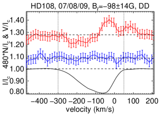
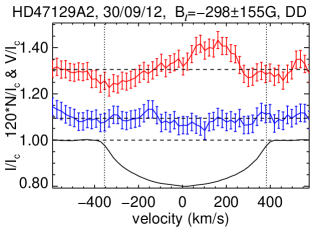
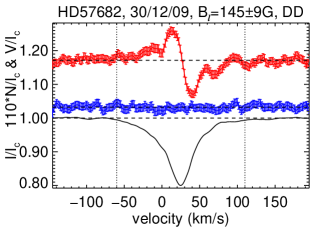
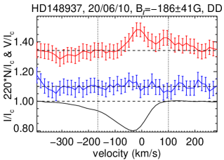
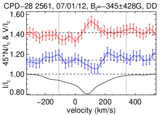
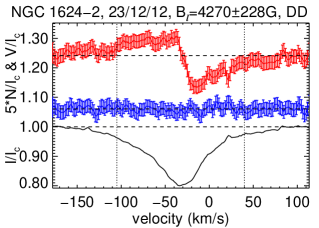
Figure 3: Example unpolarized Stokes $I$ (bottom), diagnostic null (middle) and circularly polarized Stokes $V$ (top) LSD profiles for each star considered magnetic. The detection of a Zeeman signature within the line profile of each Stokes $V$ profile with the accompanying lack of excess signal in the diagnostic null profile or outside of the line profile is used to qualify an observation as a detection. The profiles have all been rescaled such that the Stokes $I$ profile reaches a depth of 20% of the continuum and the Stokes $V$ and diagnostic null profiles have been amplified by the indicated factor. The LSD profiles for HD 47129A2 and CPD-28 2561 were constructed from the Of?p line mask discussed in the text. All other profiles were constructed from the optimal line mask. The Stokes $I$ profile for HD 47129A2 is the best-fitting profile. The name, observation date, longitudinal magnetic field with corresponding uncertainty, and detection diagnosis is indicated for each profile. Vertical dotted lines are included to show the adopted integration range for each profile. The profiles have been smoothed over 3 pixels and expanded by the indicated amount for display purposes.

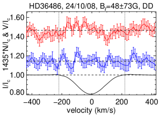
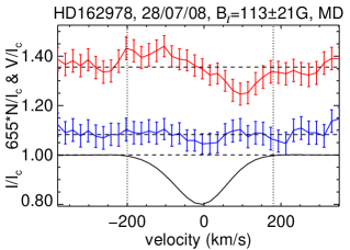
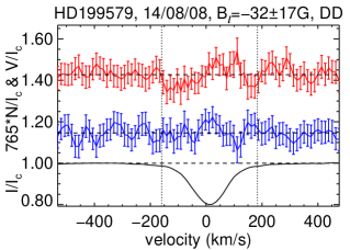
Figure 4: Same as Fig. 3 for each star that may possibly be magnetic. See Fig. 3 for further details.

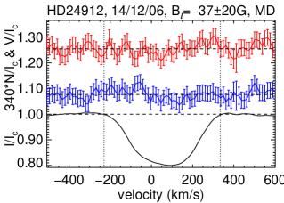
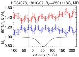
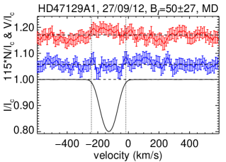
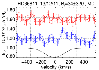
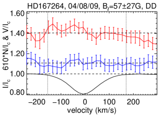
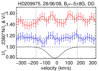
Figure 5: Same as Fig. 3 for each star that is considered to be a spurious detection. The Stokes $I$ profile for HD 47129A1 is the best-fitting profile. See Fig. 3 for further details.

Notes for particular stars (following the order presented in Table 4) are provided below.

• HD 108: Excess signal is detected outside of the line profile of one of the MDs (2008-10-26). In this case we suspect that the excess signal is residual incoherent polarization left over from the imperfect profile extraction.

• HD 47129A2 (Plaskett’s star): is a well-known multiple star system consisting of two similar O-type stars, one that exhibits relatively narrow lines (the component A1) and one component that hosts relatively broad lines (the component A2; see Appendix A for additional details). From the FAP analysis, we obtain 3 MD with the optimal line mask. Alternatively, using the simpler Of?p line mask (as employed by Grunhut et al. 2013 and Grunhut et al. in prep), we obtain 6 DD and 4 MD. This likely reflects the fact that the optimal line mask is better tailored for the component with stronger lines - in this case the narrow-line component. The Of?p line mask generally includes the strongest lines of the broad line component, and so the polarization signal is less diluted by contamination from the narrow line component. No magnetic field is confidently detected for the narrow line star (see discussion below).

• CPD-28 2561 (CD-28 5104): With the FAP analysis, we obtain 1 MD using the optimal line mask. Using the Of?p line mask we obtain somewhat better results with 3 MD, but using the Donati et al. 1997 code results in 1 DD and 6 MD. Other than HD 47129A2, this is the only star for which adoption of the Of?p line mask results in a systematic improvement in our ability to detect a Zeeman signature.

• HD 36486 ($\delta$ Ori A): is an eclipsing binary system with a close visual companion (e.g. Harvin et al., 2002). Two observations were obtained of this system on consecutive nights in 2008-10, from which we could not disentangle the individual components. We therefore discuss the results from the blended profile. A DD is obtained for the second observation (2008-10-24), which has a significantly higher S/N relative to the first observation (2008-10-23). We note that the profiles extracted with the Donati et al. (1997) LSD code both result in a ND. With only two observations, we cannot reliably confirm nor deny the presence of a magnetic field in this star. However, the lack of obvious emission in the typically strong magnetospheric emission lines of magnetic O-type stars (e.g. Balmer lines such as H$\alpha$, He ii $\lambda$4686, see e.g. Grunhut et al. 2012a) could argue against this star hosting a large-scale magnetic field. If the global magnetic field is sufficiently weak though, we may not expect strong emission. While the well-known magnetic star $\delta$ Ori C is nearby, it is sufficiently separated such that we do not expect any contamination in our observations of this star.

• HD 162978 (63 Oph): was observed 2 times: the first observation (2008-07-28) results in a MD and a $\sim$5$\sigma$ detection significance of the longitudinal field ($B_{\ell}=111\pm 23$ G). The star was reobserved several years later (2012-06-21) with approximately twice better S/N ($B_{\ell}=-13\pm 14$ G), but we do not confirm the presence of signal in the Stokes $V$ profile from that observation (the FAP analysis results in a ND). This star also exhibits uncharacteristically weak emission in key lines in which magnetospheric emission would be expected. However, we do note that the first observation in which signal was detected shows a higher level of emission relative to the second observation with a non-detected field. This behaviour could be naturally explained by a magnetic star if the magnetic pole was oriented closer to our line of sight in the first observation compared to the second, and the magnetically confined wind, which is more confined to the magnetic equator, were viewed more face-on (e.g. Sundqvist et al., 2012). We therefore consider this star a highly probable magnetic candidate.

• HD 199579 (HR 8023): Is a binary system that was observed a single time (2008-08-15). The profiles of this observation are sufficiently entangled that we could not extract individual profiles for each component and instead discuss the results of the blended profile. The FAP analysis results in a DD (a MD is obtained with the Donati et al. LSD code). This star exhibits an asymmetric absorption profile in H$\alpha$, which could be indicative of weak magnetospheric emission.

• HD 24912 ($\xi$ Per): The FAP measured from one of the profiles provides a MD (2006-12-14). Several other observations were obtained with similar S/N as the MD observation, yet no formal detections are found in any of those profiles. The profile with the MD does not present any obvious Zeeman signature in Stokes $V$. Considering this fact and the larger number of NDs, we conclude that the detection is spurious. HD 24912 is also a known non-radial pulsator, with a 3.5 h pulsation period and weak spectroscopic variability associated with this phenomenon (de Jong et al., 1999). The pulsation is likely responsible for the asymmetric Stokes $I$ line profile (see Fig. 5), and may be responsible for the spurious signal, if it were accompanied by other issues, as previously discussed. Similar results and conclusions for this star were obtained by David-Uraz et al. (2014).

• HD 34078 (AE Aur): The FAP of one of the binned profiles (2007-10-18) results in a MD; however, a MD with a similar FAP is obtained outside of the line profile in Stokes $V$ as well. No obvious Zeeman signature can be seen in the Stokes $V$ profile.

• HD 47129A1 (Plaskett’s star): One of the binned profiles of the narrow line component (A1; 2012-09-27) results in a MD based on the FAP analysis. The broad line profile of that same night also results in a MD. Given that the narrow line profile is blended with the broad line profile at all phases, its Stokes $V$ profile is contaminated by the broad line component. In fact, the detected signal appears to be part of a broader Zeeman signature that extends well outside the limits of the line profile, which is attributed to the broad line component (as shown in Fig. 5). A more thorough analysis by Grunhut et al. (in prep) shows that there is no apparent signal associated with the narrow line component.

• HD 66811 ($\zeta$ Pup): A MD is obtained from the FAP analysis for the first observation (2011-12-13) (a ND is found using the Donati et al. LSD code). A DD is also obtained within the null profile for the first observation. The second observation taken a few months later (2012-02-13) had a similar S/N but results in a ND. Since a detection is also found in the null profile, this leads us to consider the Stokes $V$ detection to be spurious. Similar results were also obtained by David-Uraz et al. (2014).

• HD 167264 (15 Sgr): Despite the similar precision of all the observations, only the FAP analysis of the profile of a single night (2009-08-04) results in a DD (a ND is obtained using the LSD code of Donati et al.). Visual inspection of the Stokes $V$ LSD profile reveals some coherent structure that could be evidence of a Zeeman profile, although the potential signature extends well outside the line profile, suggesting it is likely spurious.

• HD 209975 (19 Cep): One observation (2008-06-27) results in a $\sim$$3.1\sigma$ significance ($B_{\ell}=24\pm 8$ G); however, the FAP analysis of this observation results in a ND. The observation obtained on 2008-06-28 results in a DD (a ND is obtained using the LSD code of Donati et al.). The Stokes $V$ profile shows structure that could be indicative of a Zeeman signature, but this structure also extends outside of the line profile and therefore is likely spurious. Similar results were also reported by David-Uraz et al. (2014).

5 Discussion

5.1 Quality assessment

In this section, we discuss the quality and reliability of our data, and how that may relate to spurious detections, and possible biases. We do not address the potential for missed fields, as this will be discussed in the forthcoming paper in this series.

In Fig. 6, we show the cumulative distribution of the longitudinal field uncertainty ($\sigma$) as a representation of the precision achieved in this study. We find that about 25% of our observations achieved a $\sigma$ of 20 G or better. As some stars were observed more than once, we note that this precision was achieved for 34 different targets. Approximately 50% of our sample of observations (76 different targets) was acquired with a $\sigma$ of 50 G or less, or about 70% (101 targets) with 100 G or better. The quality achieved in this study represents the most magnetically sensitive probe of the largest sample of O-type stars to date.

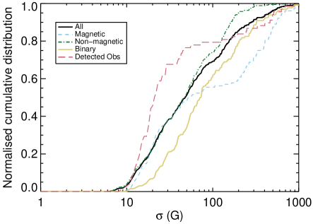
Figure 6: Cumulative distribution of longitudinal field uncertainty $\sigma$ for different samples of observations (as indicated by the included legend). The magnetic sample includes all observations corresponding to the stars deemed confidently detected as magnetic. The non-magnetic sample includes all observations of stars that are not considered confidently detected. The binary sample includes all binary stars for which the different line profiles could be disentangled. The detected sample includes only those observations for which a signal was detected in Stokes $V$.

One quality check that we performed was to investigate the precision of the data (including instrumental, reduction, and measurement systematics), by analysing the distribution of significances of the longitudinal magnetic field measurements relative to the estimated uncertainties. In Fig. 7, we show the distributions for both the confirmed magnetic sample and the unconfirmed/non-detected sample (which includes potential and spurious detections) for all stars. The measurements computed from the Stokes $V$ profile ($B_{\ell}/\sigma$) and the diagnostic null profiles ($N_{\ell}/\sigma$) are both included in this figure.

The first important conclusion is that the measurements obtained from the diagnostic null profiles from both the magnetic and non-magnetic sample (a total of 483 profiles) are consistent with a Gaussian distribution centred around a significance of 0, and all values are within $\pm 3\sigma$. The next important conclusion is that the $B_{\ell}$ measurements of the non-magnetic sample (including unconfirmed magnetic stars) are consistent with the null measurements. A two-sided Kolmogorov-Smirnov (KS) test supports the hypothesis that the non-magnetic sample of observations is drawn from the same underlying distribution - this hypothesis is not ruled out at about 2$\sigma$ confidence. This is not true for the $B_{\ell}$ measurements from the magnetic sample, which show clear differences from the null distribution. We warn the reader to avoid over-interpreting the preference for negative $B_{\ell}$ values from the magnetic star sample in this figure. This is a result of a large number of negative measurements for a few stars and should not be interpreted as a statistical preference for a given orientation of magnetic fields in O-type stars. We underscore that while the quality control checks show that the $B_{\ell}$ measurements are well behaved, these values are not used to establish whether an observation is considered a magnetic detection.

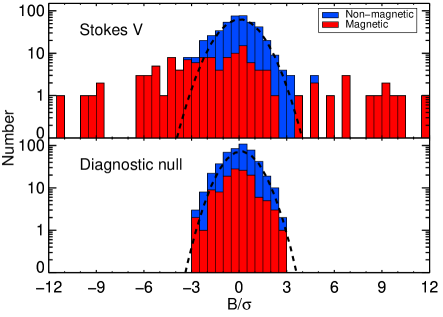
Figure 7: Top: histogram of the detection significance of the longitudinal field measurement ($B_{\ell}/\sigma$) obtained from all observations of individual stars (i.e. all non-entangled stars). Bottom: same as the top but measured from the diagnostic null profile *$N_{\ell}/\sigma$). The dashed curves represent a pure Gaussian distribution for comparison. The magnetic sample only includes all observations from stars that were confidently detected as magnetic. The non-magnetic sample includes all observation from stars that were not considered confidently detected as magnetic.

Another quality check that we performed was to assess the overall reliability of the LSD noise level of the polarimetric profiles. This is particularly important as it could provide insight into the small number of spurious detections that we encountered in our analysis, especially if we find that the noise is underestimated. We carried out a series of tests using the diagnostic null profiles, the details of which are provided in Appendix B. The overall conclusion is that, in general, the LSD uncertainties appear to be over-estimated by about 20% for the unbinned profiles. On the one hand, reducing the uncertainties by about 20% does increase the number of detections among the magnetic sample when using the unbinned profiles (37 vs 22), but this is still not as efficient as the binning strategy (61 detections). On the other hand, the uncertainty of the binned profiles are in good agreement with our expectations (they are over-estimated by $\sim$3%), although the tests show that the binning does introduce a small increase ($\sim$1.5%) in the number of FAPs from the null profiles that would be considered detections, and so some extra care must be taken when using this procedure and assessing the presence of a detectable Zeeman signature. In fact, 1.5% of the non-magnetic sample (353 observations) corresponds to about 5 observations, which is in excellent agreement with the number of detections we highly suspect as being spurious.

5.2 Biases

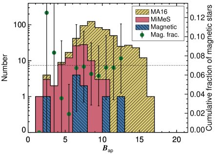
Figure 8: Histograms comparing the number of targets observed at a given approximate $B_{\rm ap}$ magnitude. Included are histograms according to the GOSSS (Maíz Apellániz et al., 2016, MA16), the targets observed in this study, and the magnetic and potentially magnetic stars identified in this work. Also shown is the cumulative magnetic incidence fraction as a function of $B_{\rm ap}$. Each bin provides the total magnetic incidence for all targets (97 in total) with a $B_{\rm ap}$ less than or equal to the indicated $B_{\rm ap}$ of the bin. The adopted magnetic incidence fraction (7%) is indicated by the horizontal dotted line, but note that the magnetic incidence fraction derived from the 97 targets, but including the potential candidates, is $8\pm 4$%.

In this section we discuss the reliability of our findings when taking into account observational biases. The first bias we consider is the reliability of our incidence rate with respect to the brightness of the selected stars in our sample. This is particularly important as two of the six confirmed magnetic stars are faint targets, and much fainter than the brightness of the general population of stars included in this study. To assess this potential issue, we compare the approximate $B$ magnitude ($B_{\rm ap}$) of our sample (e.g. Maíz Apellániz et al., 2016) to the distribution presented by the Galactic O-Star Spectroscopic Survey (GOSSS; Maíz Apellániz et al. 2016. Fig. 8 compares the histograms of the $B_{\rm ap}$ obtained from the GOSSS sample, our entire sample, and the sample of magnetic stars (including the potential candidates). We also present the cumulative magnetic incidence fraction achieved in our study, taking into account the potential magnetic candidates in this figure. In this comparison, we treat each system as an individual target to avoid potential discrepancies associated with determination of the relative brightness of each component in multiple star systems. Hence, the statistics correspond to only the 97 targets and not the total 108 individual O stars, as previously mentioned. The most obvious conclusion to be drawn from this analysis is that the incidence fraction converges to $\sim$7% with increasing magnitude. Maximum completeness of our sample of stars ($\sim$86%) is reached for $B_{\rm ap}<4$, but this only includes 6 stars. A more statistically relevant sample is reached for $B_{\rm ap}<7$, for which we achieve a completeness of 66% that includes 52 total targets in our sample, and between 2 and 4 magnetic stars (including the potential candidates). From this sample, we derive an incidence fraction of $7\pm 5$%, which is consistent with our adopted value. Including the fainter bins with a much higher magnetic incidence fraction relative does not appear to significantly affect the final incidence fraction, which leads us to conclude that our results are not sensitive to this particular observational bias.

Given the previous findings, the next outstanding question that we address here is whether there were any characteristics of the detected stars that favoured the detection of signal in the magnetic star sample versus the non-magnetic sample. This is of particular interest because it would introduce a detection bias, and it would also affect the inferred properties of the magnetic stars. One such possibility could be a result of systematically obtaining higher magnetic precision with the detected sample. We return to Fig. 6, which also shows cumulative distributions for a number of different sub-populations, to address this issue. Our first conclusion is that the distribution of uncertainties measured from the individual components of the binary sample shows a definite trend compared to the general sample of all observation - it systematically achieves a lower precision for the same relative population. This is to be expected since the S/N that we aimed for, according to the exposure time calculator described in Paper I, did not take into account binarity, so the typical magnetic precision that we achieve for each component of a binary system would naturally be lower.

Comparing the sample of observations of the magnetically confirmed stars to the non-magnetic sample, we also find some obvious differences. The samples are in excellent agreement up to about $\sigma=30$ G, before the magnetic sample’s cumulative distributions start to diverge. Surprisingly, the magnetic sample achieves substantially poorer precision than the non-magnetic sample for more than 50% of its population. Taking a closer look at the magnetic results, we find that this distribution is bimodal. The low-$\sigma$ population is dominated by many observations of HD 108 and HD 57682. HD 57682 is unique among the magnetic O-star sample as it has a rich spectrum of sharp lines, which results in higher magnetic precision at the same S/N as the other magnetic stars. The high-$\sigma$ end is populated by observations of the hot, faint stars CPD-28 2561 and NGC 1624-2, with the other stars filling in the values in between. While this comparison shows that the general population of observations of the magnetic stars achieved poorer precision than the non-magnetic sample, there are also several observations of the magnetic stars for which we did not detect excess signal. If instead we only look at the subsample of the observations with detected signatures, we do find a trend towards higher precision for about 80% of that subsample; however, these observations are again dominated by many observations of just two stars: HD 108 and HD 57682, and it is therefore difficult to draw any conclusions.

Another way to investigate any potential biases related to magnetic precision is to search for any systematic trends in the two most important factors for estimating the original exposure times: the apparent brightness and line broadening. In Fig. 9, we compare $\sigma$ to the measured total line broadening and apparent brightness for each star. In general, we find no obvious relationship between the line width and the achieved magnetic precision for most stars, except for the few stars with the very broadest lines ($v_{\rm tot}\ga 300$ km s^-1), which have larger uncertainties relative to the narrower line stars, and some of the individual components of binary systems. Furthermore, we also find no obvious relationship between the obtained precision and the brightness of the star. This result is expected as the Survey aimed to detected Zeeman signatures for field strengths between about 100 to 1000 G, which roughly translates into expected $\sigma$$\sim$$10-100$ G, for all stars in the sample.

The magnetic stars essentially fall into two groups: some stars with average precision that is in good agreement with other stars of similar brightness and line width; and the other group of stars with a magnetic precision that is generally worse than that of stars with similar line width. This former group includes most of the magnetic stars (HD 108, the broad line component of HD 47129 (A2), HD 57682, and HD 148937). The latter group includes the two fainter magnetic stars (CPD-28 2561 and NGC 1624-2), which are among the faintest stars observed in the Survey. Thus the poorer precision is a reflection of their apparent brightness and the lower achieved S/N (recall that integration times were generally kept to less than two hours). One other aspect of the magnetic stars is that several stars have a large range in their obtained precision. The relatively large range is primarily a reflection of changes in observing conditions and the corresponding S/N that was achieved for these observations, and not, for example, due to variable emission that would reduce the strength of Stokes $I$.

Therefore, based on the above discussion, we conclude that there are no obvious biases that would account for the detection of excess signal in the magnetic sample versus the non-magnetic sample.

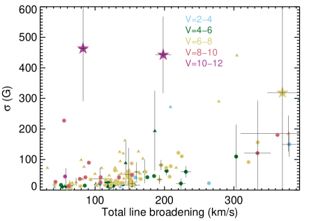
Figure 9: Measured longitudinal field error bar $\sigma$ vs total line width. The plotted data points correspond to the median value obtained for each star, and the error bars correspond to the standard deviation of the values. Different colours correspond to different magnitude bins (as indicated), while different symbols correspond to different sub-populations (circles: single stars, triangles: binaries, stars: confirmed magnetic stars). The two poorest observations for CPD-28 2561 were ignored.

5.3 Comparison with magnetic results obtained in other works

In this paper we list the confirmation of a magnetic field in six O stars previously reported as magnetic by the MiMeS collaboration (HD 108, the broad line component of HD 47129 (A2), HD 57682, HD 148937, CPD-28 2561, and NGC 1624-2), in addition to the three already known magnetic O stars discovered before this Survey ($\theta^{1}$ Ori C, $\zeta$ Ori A, and HD 191612). Three of the six new magnetic O stars have been observed by other authors and confirmed to be magnetic (Hubrig et al., 2008; Hubrig et al., 2010, 2011c; Hubrig et al., 2012b; Hubrig et al., 2013, 2015).

As previously discussed, a magnetic field detection has also been obtained with low-resolution FORS data for the O star Tr16-22 by Nazé et al. (2012) and confirmed by Nazé et al. (2014), and for the O star HD 54879, which was also confirmed with high-resolution spectropolarimetry (Castro et al., 2015). These two targets have not been observed within the MiMeS Survey, but their magnetic detections are convincing and therefore there is little doubt that they are indeed magnetic.

While a number of magnetic field detections have been claimed in 20 other O-type stars (Hubrig et al., 2007a; Hubrig et al., 2008, 2011b, 2012a; Hubrig et al., 2013; Hubrig et al., 2014), doubts had already been cast by other authors on the validity of these claims. In particular, Bagnulo et al. (2012) showed, using the same FORS data as Hubrig et al. (2008), and focusing in particular on the evaluation of realistic uncertainties, that 4 O stars previously claimed to be magnetic by Hubrig et al. were not magnetic: HD 36879, HD 152408, HD 155806, and HD 164794. In the same way, again using the same FORS data, Bagnulo et al. (2012, 2015) showed that the claims of a field in $\zeta$ Oph (Hubrig et al., 2011b) and 15 Mon (Hubrig et al., 2013) are also spurious.

Of those 20 O stars claimed to be magnetic, 12 were analysed in this work (the results for each star can be found in Appendix C). In most cases, the magnetic precision in this study exceeded that of previous measurements that led to claimed detections. No evidence of a large-scale magnetic field was found for any of these stars. For 6 of these stars, the FORS data were also re-analysed by other teams, and all were refuted as magnetic stars (Bagnulo et al., 2015).

Only 5 O stars ($\theta^{1}$ Ori C, HD 148937, CPD-28 2561, Tr16-22, and HD 54879) have been measured to be magnetic with FORS data and are confirmed to be magnetic O stars. This means that about 75% of the claimed magnetic detections among O stars using FORS are considered spurious. This percentage is consistent with the 80% spurious detections among O stars observed with FORS, as found by Bagnulo et al. (2012). Eight stars claimed to be magnetic from FORS observations have not been observed or analysed yet by independent teams, but considering the statistics exposed above, the claimed magnetic fields in these 8 stars should be considered with great caution.

Notes for particular stars previously claimed as magnetic and included in this Survey are provided below.

• HD 47839 (15 Mon) is a multi-line spectroscopic binary that was observed 8 times between 2006-12 and 2012-03, with the majority of these observations being acquired between 2007-09 to 2007-11. A ND is obtained for each component, and for each observation, but we note that the primary component dominates the line flux.

• HD 66811 ($\zeta$ Pup) was previously discussed in Sect. 4.1.

• HD 153426 is a spectroscopic binary that was observed twice between 2011-07 and 2012-07. A ND is obtained for each component. The primary component dominates the line profile.

• HD 155806 was observed 4 times between 2008-06 and 2008-08. No formal detection of excess signal was found for any of the observations (see also Fullerton et al. 2011). The $B_{\ell}$ measurement from one of our observations results in a 3.2$\sigma$ detection ($B_{\ell}=-44\pm 14$ G; 2008-06-25), but no evidence of nonzero $B_{\ell}$ is obtained from the other observations with similar precision.

• HD 164794 (9 Sgr) is a spectroscopic binary that was observed 5 times between 2005-06 and 2011-07. We were not able to disentangle the two components and therefore we report the results for the blended profile. Hubrig et al. (2013) presented results based on publicly available HARPS data collected within the MiMeS HARPSpol LP. Their analysis resulted in a $B_{\ell}=210\pm 42$ G ($B_{\ell}/\sigma\sim 5$) from this data, while our analysis of the same data results in a substantially lower field measurement of $B_{\ell}=-1\pm 48$ G ($B_{\ell}/\sigma\sim 0$), despite having similar uncertainties.

The total number of known and confirmed magnetic O stars at the time of writing is thus 11: HD 108, the broad line component of HD 47129 (A2), HD 54879, HD 57682, HD 148937, HD 191612, CPD-28 2561, NGC 1624-2, Tr16-22, $\theta^{1}$ Ori C, and $\zeta$ Ori Aa.

5.4 Searching for trends

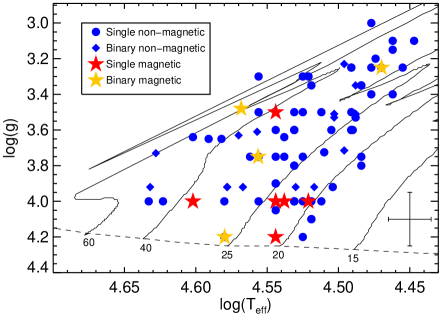
Figure 10: $\log(g)-T_{\rm eff}$ diagram showing the position of all stars studied here in addition to other confirmed magnetic O stars ($\theta^{1}$ Ori C, $\zeta$ Ori Aa, Tr16-22, HD 54879, HD 191612). Evolutionary tracks of Ekström et al. (2012) are also included. The blue loops of some of the evolutionary tracks are neglected for display purposes. Note that there are several overlapping symbols due to different stars with similar properties. The size of the typical error bars is indicated in the figure.

One of the ultimate goals for a study of this nature is to identify a link between a physical or phenomenological property and massive O-type stars hosting large-scale, strong magnetic fields. This idea is well established for late-type stars as there is a direct correlation between the observed magnetic field strength and certain activity indicators (e.g. Ca ii H&K core emission, X-ray emission, etc.), which probe the coronal or chromospheric emission that is modified by the presence of a magnetic field (e.g. Noyes et al., 1984). Similarly, among the intermediate-mass A and B stars that host strong magnetic fields, distinct chemical peculiarities are observed that make these stars easily identifiable - the so called Ap/Bp stars (e.g. Donati & Landstreet, 2009). Martins et al. (2012a); Martins et al. (2015) already investigated the correlation between CNO abundance peculiarities among the magnetic O-type stars compared to the non-magnetic O-type stars and found no obvious distinctions between the two different populations. We therefore look into other physical or phenomenological properties.

The first aspect we investigate is whether there are any correlations between physical properties and magnetism in the attempt to identify regions of the Hertzsprung-Russel (HR) diagram that would be more likely to host magnetic stars, similar, for example, to the pulsational instability strips. In Fig. 10, we present a $\log(g)-T_{\rm eff}$ diagram that contains all the stars studied here in addition to other confirmed magnetic O stars ($\theta^{1}$ Ori C, $\zeta$ Ori Aa, Tr16-22, HD 54879, HD 191612). The $T_{\rm eff}$ and $\log(g)$ values for each star are taken from Martins et al. (2015) (when available) or were estimated based on their spectral type according to the study of Martins et al. (2005a). The parameters adopted for HD 54879 were taken from Castro et al. (2015), while the parameters for NGC 1624-2 adopted the results of Wade et al. (2012b), and the parameters for $\zeta$ Ori Aa were taken from Blazère et al. (2015). This figure is an update to that presented by Martins et al. (2015), now containing all known magnetic O stars (11) and all the O stars studied in this work. Even with the inclusion of several additional magnetic O stars, our conclusion mirrors that of Martins et al. - there appears to be no correlation between physical properties (e.g. $M$, $T_{\rm eff}$, $\log(g)$ and therefore $L$, $R$ and age) and the presence of magnetic fields in O-type stars. While there are no obvious correlations, we do point out that majority of known magnetic O-type stars are concentrated on the first half of the main sequence. The only star that is more evolved is the supergiant $\zeta$ Ori Aa, which is close to the terminal age main sequence. This could be related to the decrease of the surface field strength with increasing radius as the star evolves, due to magnetic flux conservation.

Motivated by the results of Landstreet et al. (2007) and Fossati et al. (2016) that show evidence for magnetic field decay, we attempted to search for any correlation between age and surface magnetic field strength. To do so, we followed a similar strategy as adopted by Landstreet et al. (2007) and looked at the correlation between the $B_{rms}$ parameter (derived from $B_{\ell}$ measurements found in this work, and from $B_{\ell}$ measurements reported in the dedicated studies of these individual stars) and $\log(g)$, which we used as a proxy for age. We also looked at the correlation of $\log(g)$ with surface dipole field strength, based on results of the dedicated studies of the individual magnetic O stars. Unfortunately, the majority of the magnetic stars have $log(g)\sim 4$ and host a large range of field strengths (several hundreds to thousands of G). Other than $\zeta$ Ori Aa, the magnetic stars with $log(g)\la 4$ have similar field strengths to those measured from stars with $log(g)\sim 4$, so no obvious conclusions can be made. The only star that shows evidence for a decrease of magnetic field strength with age is $\zeta$ Ori Aa, which is the most evolved magnetic star in this sample and also hosts the weakest field.

Another important aspect that we investigate is the correlation between rotation rate and the presence of a magnetic field. It is well established that main sequence and pre-main sequence magnetic A and B stars generally rotate at a fraction of the speed of non-magnetic A and B stars (e.g. Donati & Landstreet, 2009; Alecian et al., 2013), likely as a result of the shedding of angular momentum due to magnetic coupling to the stellar wind and/or circumstellar disk during star formation (e.g. Stȩpień, 2000). To address this aspect, we present a histogram of the rotation periods for each O-type star in our sample, in addition to all confirmed magnetic O stars (see Fig. 11). For the magnetic stars, we adopted the rotation periods inferred from their photometric, spectroscopic, or $B_{\ell}$ variations from previous studies. Since we do not have independent measurements of the rotation periods for the non-magnetic stars, we therefore estimated the rotation periods of these stars assuming rigid rotation using our $v\sin i$ measurements and typical radii according to their spectral types, based on the study by Martins et al. (2005a). For stars with multiple measurements, we used the median $v\sin i$. The rotation period was also estimated in this way for HD 54879, using the radius ($6.7^{1.0}_{-0.9}$ $R_{\odot}$) and $v\sin i$ ($7\pm 2$ km s^-1) of Castro et al. (2015). We assumed $\sin i=1$ when obtaining the rotation periods to obtain maximal values (this also reduces the potential bias from our profile fitting that could over-estimate the contribution of $v\sin i$ to the line profile). While the individual rotation periods of the non-magnetic stars are highly uncertain, as a collective they are more robust, and the distribution is sufficient for the purposes of this discussion.

The full interpretation of the results presented in Fig. 11 is outside the scope of this paper, but we can make some general conclusions. The first conclusion is that the distribution of rotation periods for the magnetic stars is very different from that of the non-magnetic stars (a two-sided KS test supports the hypothesis that the magnetic sample is not drawn from the same underlying distribution as the non-magnetic sample - the null hypothesis that the two distributions are drawn from the same sample is rejected at 99.9% confidence). The most significant conclusion is that the majority (60%) of the magnetic stars have rotation periods longer than the longest periods found in the population of non-magnetic stars (stars with rotation periods $\ga$50 d all appear to be magnetic). We can therefore conclude that magnetic fields play a very important role in explaining the rotation among the slowest rotating O-type stars. However, there still exists a population of magnetic stars with rotation periods comparable to the periods found from the non-magnetic stars. As discussed by ud-Doula et al. (2009), angular momentum loss depends on several key physical parameters of the star such as the magnetic field strength, the mass-loss rate, the rotation rate, and the radius. Therefore, to interpret the current rotation period of the star one needs to take all these factors into account, in addition to the age of the star (the older the star, the longer the star may have been affected by angular momentum loss).

The magnetic stars with the shortest rotation periods are: the broad line component of Plaskett’s star (1.21551 d - Grunhut et al. in prep); $\zeta$ Ori Aa (6.83 d - Blazère et al. 2015); HD 148937 (7.03 d - Nazé et al. 2008; Wade et al. 2012a); $\theta^{1}$ Ori C (15.442 d - see Wade et al. 2006, and references therein). The more rapid rotation of these stars relative to the other magnetic O stars is likely a reflection of one (or several) of the following reasons: the age (an insufficient amount of time has passed to carry away enough angular momentum); the magnetic field strength is much weaker than other magnetic O-type stars and therefore couples more weakly to the stellar wind, which reduces the angular momentum loss; some form of angular momentum transport has occurred due to binary interaction, which has rejuvenated the star. This topic will be addressed in a future paper in this series.

Given the tendency to overestimate the rotational contribution to line profiles of magnetic stars (e.g. Sundqvist et al., 2013), it may very well be that the rotation rates of the non-magnetic stars are also over-estimated and therefore the rotation periods are under-estimated; however, if we compare to the $v\sin i$ distribution of all stars instead of their rotation periods, we arrive at a very similar result, except that the $v\sin i$ of HD 108 is considerably over-estimated in this study (see e.g. Martins et al., 2010, Shultz et al. in prep).

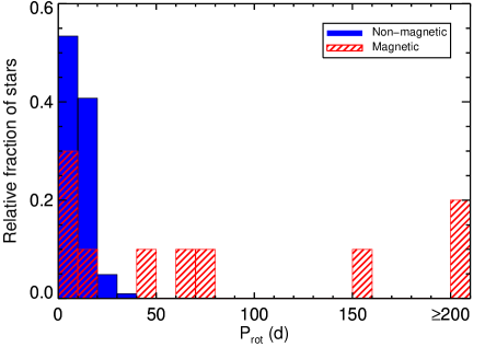
Figure 11: Histogram of the O star rotation periods. The rotation periods of the magnetic stars were taken from the literature, while the periods of the non-magnetic stars were estimated from their $v\sin i$ measurements and radii according to their spectral types.

We next attempt to link an observable phenomenon to the presence of magnetic fields, by looking at the incidence rate of magnetism among a number of different subsamples.

5.4.1 Oe stars

Oe stars are a subset of O-type stars that currently exhibit, or at some point in their history have exhibited, emission in their spectra, typically in the Balmer lines. As recent studies have suggested a much higher incidence of magnetic fields among early-type emission line stars, this group is of particular interest (e.g. Hubrig et al., 2007b; Hubrig et al., 2009).

A careful examination of all our spectra revealed evidence of emission in the H$\alpha$ Balmer line for 47 of our targets, including all stars with a confirmed magnetic field. This results in a somewhat higher magnetic incidence fraction among emission line O stars of $13\pm 6$%, but by no means indicates a direct link between emission and magnetic fields. This result is not surprising as a number of different physical mechanisms could be responsible for producing emission in these sources (e.g. wind emission, wind-wind collision, magnetosphere, decretion disks, etc).

Of particular interest among the Oe stars are the classical Oe stars (Conti & Leep, 1974), which have been suggested to be a magnetic phenomenon (for example, the magnetically torqued disk model; Cassinelli et al. 2002). The characteristics of their line emission is generally morphologically distinct from other emission line stars and is attributed to a circumstellar decretion disk, usually considered to be a continuation of the Be phenomenon towards hotter spectral types (see Porter & Rivinius, 2003; Rivinius et al., 2013, for further details of the emission characteristics of Be stars).

Out of the 8 prototypical classical Oe stars proposed by Frost & Conti (1976), only two were observed in the context of the MiMeS survey: HD 155806 and HD 149757, which were both discussed in the previous section and are not found to be magnetic. Additionally, the Be Star Spectra (BeSS) database contains a catalogue of all known $\sim$2000 confirmed or suspected classical and Herbig Oe and Be stars, as well as a collection of more than 100 000 spectra provided by professional and amateur astronomers (Neiner et al., 2011). If we include all the stars with an O-type classification present in this database, there is a potential sample of about 70 stars. Unfortunately, only a few of these additional stars were analysed by the MiMeS Survey (HD 17505, HD 24912, HD 37041, HD 57682). Of the total sample of possible classical Oe stars analysed here, only HD 155806 exhibits an emission morphology consistent with a classical Oe star. The others either show no obvious emission (HD 17505), only minor core emission (HD 24912, HD 149757), or their emission is attributed to other phenomena (HD 37041 is nebular; HD 57682 is magnetospheric - see Grunhut et al. 2012a for further details) during the epoch of observation. Therefore, with the very limited sample of classical Oe stars available in this work, there is no evidence of a direct connection between magnetism and the classical Oe phenomenon. A more statistically significant study will be required to determine if classical Oe and Be stars are as magnetic or less magnetic than normal O-stars, and this is the subject of a future paper in this series (Neiner et al. in prep); however, a preliminary analysis carried out by the MiMeS collaboration indicates that Be stars have a lower magnetic detection rate relative to non-Be stars (Wade et al., 2014).

5.4.2 “Weak-wind” stars

“Weak-wind" stars are O-type dwarfs that have anomalously lower observationally derived mass-loss rates (by a factor of $\sim$100), and terminal wind velocities that are also found to be lower than theoretical predictions determined from their luminosity (e.g., Martins et al., 2004, 2005b; Marcolino et al., 2009; Martins et al., 2012b). This behaviour occurs for stars with $\log{\rm L}/\rm{L_{\odot}}<5.2$, and is found for both solar and lower metallicity objects. While no current solution exists to explain such behaviour, Martins et al. (2005b) suggested that magnetic fields may significantly alter the ionisation structure, which would reduce the mass-loss rates and terminal wind velocities. The discovery of a magnetic field in several early-B stars (e.g. $\zeta$ Cas Neiner et al. 2003a, V2052 Oph Neiner et al. 2003b, 2012a) and in the weak-wind O9 IV star HD 57682 (Grunhut et al., 2009, 2012a) has provided additional support for the possibly important role of magnetic fields to explain this phenomenon.

Included in our survey are six additional targets that have been identified as so-called “weak wind” stars by Martins et al. (2005b) or Marcolino et al. (2009): HD 37468, HD 38666, HD 46149, HD 46202, HD 66788, HD 149757. Our observations provide no evidence for the presence of a magnetic field in any of these stars. Results for each star can be found in Appendix C.

The lack of detection in any of the other weak-wind stars in this survey highly suggests that strong, large-scale magnetic fields do not play an important role in this phenomenon. This is further supported by recent MHD simulations of ud-Doula et al. (2008) that have shown that the presence of a strong, large-scale magnetic field can reduce the mass carried away by the stellar wind by around 90%. This is in poor agreement with the orders of magnitude drop in the observed mass-loss rates. The more likely explanation is related to issues with how mass-loss rates are measured (e.g. Huenemoerder et al., 2012), or with the theoretical predictions (e.g. Muijres et al., 2012).

5.4.3 Runaway stars

Recent studies suggest a high incidence of candidate runaways among known magnetic O stars, possibly implying that the detected magnetic fields are generated or acquired during the ejection process (e.g. Hubrig et al., 2011c). Exploration of the runaway status of all stars analysed here is outside the scope of this current study, but it is worth mentioning that only 3 of the original 7 stars identified as magnetic and runaway candidates by Hubrig et al. (2011a) should be considered runaway candidates at $>$$1\sigma$ significance (HD 108, HD 152408, HD 191612). HD 152408, which was previously discussed, shows no evidence of the presence of a magnetic field in this study or by Bagnulo et al. (2012). Four additional candidates of this subclass were presented by Hubrig et al. (2011c), and of those 4, 3 were analysed in this study and show no evidence of the presence of a magnetic field (HD 153426, HD 153919, HD 154643). Therefore, it is unlikely that magnetic fields generated or acquired during the ejection process are a viable origin for magnetism in O-type stars.

5.4.4 Of?p stars

Of the currently identified magnetic O stars, 5 are associated with the peculiar spectral classification “Of?p". This classification was first introduced by Walborn (1972, 1973) according to the presence of C iii $\lambda 4650$ emission with a strength comparable to the neighbouring N iii lines. Well-studied Of?p stars are now known to exhibit recurrent, and apparently periodic, spectral variations (in Balmer, He i, C iii and Si iii lines), narrow P Cygni or emission components in the Balmer lines and He i lines, and UV wind lines weaker than those of typical Of supergiants (see Nazé et al., 2010, and references therein).

Our sample includes all 5 of the known (Walborn et al., 2010) Galactic Of?p stars: HD 191612, HD 108, HD 148937, NGC 1624-2, and CPD-28 2561. All but HD 191612 (detected as magnetic by Donati et al., 2006, and included in the TC) were survey targets. Many of these stars are relatively faint and would not have been considered as suitable survey targets, but were included as a consequence of the known field of HD 191612.

Our investigation establishes that the Of?p stars represent a distinct class of magnetic O-type stars. It therefore appears that the particular spectral peculiarities that define the Of?p classification are a consequence of their magnetism. The analogous periodic photometric and spectroscopic variability of several Of?p stars discovered in the Magellanic Clouds (Nazé et al., 2015; Walborn et al., 2015) provides further support to their magnetic nature (all well-studied magnetic O-type stars are known to exhibit period variability, which is a consequence of rotational modulation of their confined winds).

Detailed investigations of the magnetic field and wind properties of the Of?p stars have been published by Martins et al. (2010), Wade et al. (2011); Wade et al. (2012a, b), and Hubrig et al. (2015).

6 Summary

The MiMeS LPs acquired about 500 high-resolution, high-S/N spectropolarimetric Stokes $V$ sequences of O-type stars with ESPaDOnS, Narval, or HARPSpol. An additional $\sim$380 spectropolarimetric Stokes $V$ sequences were collected from the public archives corresponding to each instrument/observatory. In the end we obtained high-resolution spectropolarimetric Stokes $V$ sequences for 97 O-type star systems.

After co-adding all sequences of a given target obtained on a given night, we ended up with 416 individual polarized spectra of the 97 targets. Mean LSD Stokes $I$, Stokes $V$ and diagnostic null profiles were extracted from each spectrum using a number of different line masks. Ultimately, we concluded that line masks individually tailored for each spectrum were the most suitable for the detection of signal resulting from a Zeeman signature.

For each of the extracted mean LSD Stokes $I$ profiles, we attempted to constrain their basic spectral properties (e.g. $v_{r}$, $v\sin i$, $v_{\rm mac}$) through the use of an automated tool. These results can be found in Appendix C. In the process of fitting each profile, we encountered several profiles that showed obvious signs of multiplicity or were previously known multi-line spectroscopic systems. In these cases we simultaneously fit the profiles of all components, when possible, and used these fits to extract individual profiles of each star. This procedure also led to the discovery of 2 new possible spectroscopic companions for HD 46106, and HD 204827, and the confirmation of a spectroscopic companion for HD 37041.

Taking into account the multiple star systems, we therefore performed a magnetic analysis on 108 O-type stars. With a median precision of the $B_{\ell}$ measurements of 50 G (25% of the observations were acquired with $\sigma$$<$20 G and 70% with $\sigma$$<$100 G), this is the most magnetically sensitive study of the largest sample of O-type stars carried out to date. The MiMeS survey discovered or confirmed the presence of a magnetic field in 6 O-type stars: HD 108, the broad line component of HD 47129 (A2), HD 57682, HD 148937, CPD-28 2561, and NGC 1624-2. An additional 3 stars (HD 36486, HD 162978, HD 199579) show evidence suggesting the presence of a magnetic field, but we lack the data to confirm these suspected fields. Based on these results, we derive a magnetic incidence fraction of $7\pm 3$% among the observed O-type stars. This is substantially lower than other previous claims obtained, in general, with low-resolution spectropolarimetry (e.g. $\sim$30%; Hubrig et al., 2011c). Furthermore, we were not able to confirm the presence of a magnetic field in 12 stars that were previously claimed to be magnetic by others. This is in good agreement with an independent reanalysis of the low-resolution FORS data by Bagnulo et al. (2012), who were not able confirm the majority of magnetic claims among the FORS archival data.

The majority of magnetic O stars are located in the first half of the main sequence ($\zeta$ Ori Aa is the only exception, as it currently resides close to the terminal age of the main sequence). Besides this qualitative observation, we found no correlation between the presence of a magnetic field and the physical properties of the star (e.g. $T_{\rm eff}$, $\log(g)$, $M$, or age). While there is no direct correlation between the rotation period of a star and the presence of a magnetic field, the majority of the confirmed magnetic stars are found to be rotating much slower than non-magnetic stars. The slower rotation likely results from enhanced angular momentum loss due to magnetic coupling with the stellar wind, which is expected to rapidly decrease the angular rotation rate of the star within a few million years (e.g. ud-Doula et al., 2009). In fact, detailed studies of the magnetic O-type stars show convincing evidence for the presence of co-rotating, magnetically structured winds, the presence of which agrees well with theoretical or numerical expectations between the coupling of the magnetic field and wind (e.g. Grunhut et al., 2012a, 2013; Sundqvist et al., 2012; Wade et al., 2011; Wade et al., 2012a, b; Wade et al., 2015).

We also explored the incidence of magnetic fields for certain subclasses of stars that present different phenomenological characteristics (e.g. “weak-winds", emission). No direct correlation could be found between the phenomena that define most subclasses and the presence of a magnetic field.

The only subclass for which we were able to identify a direct link with the presence of magnetic fields is the peculiar Of?p stars. All 5 of the known Galactic Of?p stars were included in this survey and all were found to be magnetic. We therefore establish that the Of?p stars represent a distinct class of magnetic O-type stars, similar to the intermediate-mass, chemically peculiar Ap/Bp stars.

This paper presents the magnetic results for all O-stars studied as part of the MiMeS Survey. In the next paper in this series, we will study the null results in more detail. This will allow us to address issues such as fields below our detection threshold, the possibility of a magnetic desert, and the completeness of our survey.

Appendix A Details of the spectroscopic multiple systems

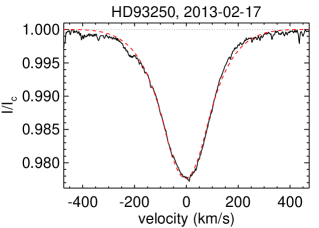
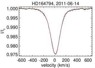
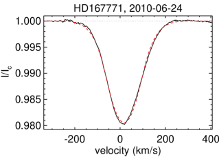
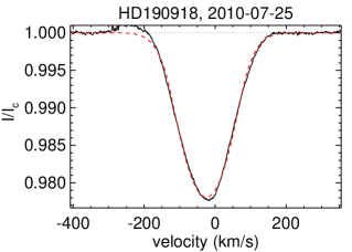
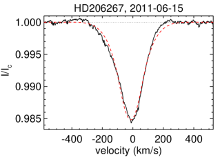
Figure 14: Example unpolarized Stokes $I$ LSD profiles for multi-line spectroscopic binaries for which we were unable to fit individual profiles to each component. The solid black line is the observed LSD profile, the dashed red line is a single star synthetic profile fit to the entangled observation. The name and observation date have been provided for each star.

This section provides a summary of the details of the spectroscopic multiple systems. In Fig. 12, we illustrate the quality of our multi-line fitting technique to the LSD profiles of each system. Fig. 14 provides a comparison between the observed LSD profile and a synthetic profile corresponding to a single star to illustrate the level of entanglement. Example profiles for HD 36486 and HD 199579 are provided in Fig. 4.

• HD 1337 (AO Cas) is a well-known close binary ($P=3.52$ d) with two O-star components (e.g. Bagnuolo et al., 1999; Palate & Rauw, 2012). The LSD profile shows two clearly separated profiles; the RV measurements of each component agree well with previous studies.

• HD 17505 is a triple system composed of three O-type stars, which was previously studied by Hillwig et al. (2006) and additional references therein. Our LSD profile shows a clearly blended profile with three obvious components. The RV measurements and other aspects of the line profiles of the three components are in good agreement with previous studies.

• HD 35921 (LY Aur) is a spectroscopic eclipsing binary with a close visual companion (ADS 4072B; e.g. Stickland et al., 1994; Mason et al., 1998). The primary component (A1) is an O star and the secondary (A2) is an early B star. Our LSD profile shows three distinct profiles - two deep and broad profiles (corresponding to the primary and secondary components) and one narrower weak component. The spectroscopic binary is well separated with the primary at positive velocities in our spectrum, in accordance with the orbital solution of Stickland et al. (1994). The reported separation of the visual companion ($\sim$0.61 arcsec; Mason et al., 1998) is small enough that it would fall in the instrument’s pupil and therefore we included an additional component for this star in our fitting procedure. We suspect that the narrow profile blended with the primary profile at an RV $\sim$-18 km s^-1 comes from the visual companion (component B), although Stickland et al. (1994) find a value of about $+25$ km s^-1. There appears to be a fourth component at very high velocities, but we suspect this is just due to residual telluric features. In fact, similar features can be seen in other profiles for different stars, but their relative strength varies. In this case, the strength of the feature is deep enough that it was attributed to another star.

• HD 36486 ($\delta$ Ori A) is a complex multiple star system consisting of an eclipsing spectroscopic binary with a $\sim$6 d period (the Aa1 and Aa2), and close visual companion (Ab) (e.g. Harvin et al., 2002; Richardson et al., 2015, and references therein). Additionally, there are two more angularly separated components B and C. The primary component of the eclipsing binary is a late O-type star and its companion is an early B-type star. There is no evidence in our LSD profiles for the presence of multiple line profiles. Any attempts at fitting our observed profiles with multiple components (using the orbital parameters of Harvin et al. 2002) failed. Given the large magnitude difference in the optical of the two stars in the close binary system ($\Delta V\sim$2.5; Harvin et al., 2002), we suspect that our LSD profile is dominated by the primary O star. Note that $\delta$ Ori C is a well-known magnetic Bp star and is separated by about 50 arcsec from $\delta$ Ori A. This separation is sufficiently large that no contamination of the observations by light of $\delta$ Ori c is possible.

• HD 37041 ($\theta^{2}$ Ori A) is part of a multiple star system with at least four components (Mason et al., 1998). The brightest component (Aa) belongs to a spectroscopic binary, which is known to have a 21 d orbital period (Aikman & Goldberg, 1974). The companion (Ab) is not spatially resolved nor detected in previous studies (e.g. Sota et al., 2011); however, Simón-Díaz et al. (2006) noted that the poor fit of their single-star synthetic line profiles to the wings of the He i lines in their observed spectrum could be caused by the presence of a companion star. The other components in this system are well separated and should not contribute at all to the observed spectrum of this star. Our LSD profiles show strong evidence for the presence of the companion as a depression in the wings of the primary profile, similar to what was observed by Simón-Díaz et al.. The parameters for the LSD profile of each component was obtained from the best fit to all observations.

• HD 37043 ($\iota$ Ori) is part of a 29 d double-lined, spectroscopic binary system in a highly eccentric orbit (Stickland et al., 1987; Bagnuolo et al., 2001). The primary is a late O-type star and the secondary is an early-type B star. Our observed LSD profile shows the secondary clearly blended with the blue wing of the primary star. We fixed the RV values to the orbital velocities from Stickland et al. (1987) to constrain our fits to the entangled profile. The resulting EW ratios of the two components are in good agreement with results of Bagnuolo et al. (2001).

• HD 37366 is a double-lined spectroscopic system in a 32 d orbit with a faint visual companion (see Boyajian et al., 2007, and references therein). The primary star is classified as a late O-type star, while the secondary is an early B-type star. Our LSD profile shows two well-separated profiles - a narrow profile at negative velocities and a very broad profile at positive velocities. The RV measurements and widths of the profiles are consistent with the study of Boyajian et al. (2007).

• HD 37468 ($\sigma$ Ori AB) is a massive triple system composed of the recently confirmed double-lined spectroscopic binary (the Aa and Ab components) and the well-known visual companion $\sigma$ Ori B that is separated by less than 0.3 arcsec from the binary system (Simón-Díaz et al., 2011, and references therein). The binary system is comprised of an O-type star and an early B-type companion (Simón-Díaz et al., 2015). Our LSD profile shows the clear presence of a narrow line profile entangled with a much broader profile. We fit our LSD profile without any constraints and found that our best-fitting values are consistent with Simón-Díaz et al. (2015). $\sigma$ Ori B was not included in our original fits. Our attempts to include this component resulted in a failure for our fits to converge. Further constraining the models using the orbital and rotational velocities determined by Simón-Díaz et al. (2015) did not improve the situation. We therefore neglected component B. This should have minimal impact on the results, as this component represents about 20% of the overall EW, or about 10% of the EW of the Aa and Ab components.

• HD 46106 is not a previously known spectroscopic binary. Our LSD profile shows strong evidence for two components - one narrow line component and one broad line component. Our RV measurement differs substantially from a previous measurement of Duflot et al. (1995) and the line asymmetry also differs from the profiles of Sota et al. (2011), both key points that further support our binarity claim.

• HD 46149 is a recently discovered spectroscopic binary composed of a late O-type star and an early B-type star (Mahy et al., 2009). Our LSD profiles show evidence for both a broad and narrow line component. We conducted our fits without any constraints and the resulting RV measurements are in good agreement with Mahy et al. (2009).

• HD 47129 (Plaskett’s star) is a well-known multiple star system consisting of a spectroscopic binary in addition to 3 visual companions at distances of 36 mas, 0.78 arcsec and 1.12 arcsec (Turner et al., 2008; Sana et al., 2014). The spectroscopic binary system was previously found to be composed of two O star components, one with narrow lines (A1) and the other showing relatively broad lines (A2), with similar RV variations (e.g. Plaskett, 1922; Linder et al., 2008); however, the recent work of Grunhut et al. (in prep) argues that the broad line component shows only weak RV variations consistent with a mean RV of about 15 km s^-1. We therefore constrained the broad line component to have a fixed RV of 15 km s^-1, but allowed all other values to vary. The resulting RV measurements for the narrow line component are in good agreement with previous studies (e.g. Linder et al., 2008). The spectral types used in this work are from Linder et al..

• HD 47839 (15 Mon) is a known speckle (with a separation of 0.035 arcsec) and single-lined spectroscopic binary system (Gies et al., 1993). The primary star has a spectral type of O7 V, while the secondary is in the range of B0-O9 (Gies et al. suspect a spectral type of O9.5 Vn, considering the breadth of the potential secondary’s lines). Our LSD profiles show evidence for stronger absorption in the red wing compared to the blue wing, which we attribute to the presence of the companion with broad lines - a result that supports the findings of Gies et al.. We constrained our fits by adopting the RV values corresponding to the orbital solution of Gies et al.. Given that these stars are of similar temperature, we use the EW ratio of the best-fitting profiles to establish a flux ratio of $\Delta m=1$, which agrees well with the lower limit of the flux ratio from a similar analysis of He i lines and the speckle observations as measured by Gies et al..

• HD 48099 is a double-lined spectroscopic binary with a short $\sim$3 d period. The system is composed of two O stars (Mahy et al., 2010). Both of our LSD profiles show evidence for the blending of two profiles. We used the predicted RV values and the rotational velocities of Mahy et al. (2010) to constrain our fits to the observed LSD profiles. The resulting best-fitting profiles are in good agreement with the results presented by Mahy et al. (2010) and provide a reasonable fit to the observed profiles.

• HD 54662 is a long period ($\sim$560 d) double-lined O-O star spectroscopic binary (Boyajian et al., 2007). Our LSD profile shows clear evidence for the presence of both a narrow and broad line component. We carried out an unconstrained fit to the LSD profile and the resulting RV measurements and line broadening for the narrow line component are consistent with previous studies (Conti & Frost, 1977; Boyajian et al., 2007). We find a higher value for the line broadening of the broad line component than Boyajian et al.. The EW ratios of the two fits are in good agreement with the flux ratio found by Boyajian et al., given that the temperatures of the two stars are similar.

• HD 93250 is a recently discovered interferometric binary system with a separation of less than 2$\times 10^{-3}$ arcsec. Sana et al. (2011) carried out a detailed investigation and found no evidence for the presence of a spectroscopic companion. It was also shown that two similar profiles separated by 50 km s^-1 could reproduce the apparently single line profile. Our LSD profile shows no convincing evidence for the presence of two blended profiles. We note that the intensity of the red wing of our LSD profile is slightly elevated relative to the blue wing, which may be an indication of a spectroscopic companion. Considering the degeneracy of potential fits, we did not attempt to fit this profile.

• HD 153426 is a known radial velocity variable star that is suspected to be an SB2 (Crampton, 1972). Our first LSD profile obtained on 2011-07-03 shows clear evidence for extended absorption in the red wing that we attribute to the presence of a very broad profile, in addition to the narrow line component. The presence of this broad profile is not apparent in the second LSD profile obtained on 2012-06-22. We fit LSD profiles assuming maximum contribution from the broad line component. This provides a good fit to our first profile, but does not fit the second profile well.

• HD 155889 is a known speckle binary with a 0.19 arcsec separation (e.g. Mason et al., 1998). Our LSD profile exhibits enhanced absorption in the red wing of the line profile, which we attribute to the presence of a spectroscopic companion, which may or may not be the speckle companion. Our fits to the LSD profile assume maximum contribution of the broad line companion.

• HD 164794 (9 Sgr) is a recently uncovered spectroscopic O-O star binary in an eccentric orbit, with a long (8.6 yr) orbital period. The study of Rauw et al. (2012) determined both the orbital and spectroscopic parameters of the secondary star. They found both components to have similar brightness and similar line widths. Our spectra were obtained at epochs where the stars have similar RVs and their spectra are highly blended. We attempted to fit our LSD profiles using the RV solution and estimated rotational velocities of the previous study, but the final results are too degenerate to find a reasonably unique solution. We therefore do not attempt to disentangle the profiles for this system and analysed the single blended profile instead. The spectral types noted in this work are from Rauw et al. (2012).

• HD 165052 is a well-known SB2 system composed of two O-type stars in a close 3 d orbit (Conti, 1974; Morrison & Conti, 1978; Stickland et al., 1997b). This system was recently investigated as part of the study of Linder et al. (2007), who found the two components to have similar spectral types and a luminosity ratio of about 1.55, in favour of the primary. This study also determined the rotational broadening parameters of each component. Our observation does not show clear evidence for two separate profiles; however, this is easily explained as we observed this star at conjunction and thus both profiles are well blended. We first attempted to fit the LSD profile using RV values for each component based on the orbital solution of Linder et al., as well as their rotational broadening measurements. While the resulting solution provided a reasonable fit to the observed LSD profile, we found a much better fit when only constraining the RV of each component. In the latter case the total line broadening for each component is considerably higher than what is reported by Linder et al. and we find the primary star to exhibit broader lines. The EW ratio of the two profiles are in good agreement with results of Linder et al. with the primary to secondary EW ratio of 1.59.

• HD 167771 is a well-known spectroscopic binary, although the secondary component was only revealed many years after the first RV variation measurements by Stickland et al. (1997a). This study found that the EW ratio (primary/secondary) of the cross-correlation function profiles from IUE data was about 1.7, with velocity widths of 115 and 85 km s^-1 for the primary and secondary, respectively. Unfortunately, our observation was taken at a phase when the two profiles are heavily blended and the observed LSD profiles appear to be that of a single star. We attempted to fit the observation using the orbital solution and rotational velocities of each component from Stickland et al.. The results were in poor agreement with the data. We next tried to fit the LSD profile using just the RV constraints from Stickland et al.. We obtained a much better fit, but the total line broadening was about 30 km s^-1 higher for the primary and about 40 km s^-1 higher for the secondary. We furthermore found that the EW ratio of the two profiles was closer to 1.5 than the expected 1.7. Considering the degeneracy involved when fitting these highly blended profiles we chose not to utilise our fits in any measurements.

• HD 190918 is a well-known WR+O binary system with several faint, nearby visual companions (e.g. Hoffleit et al., 1983; Mason et al., 2001). The WR+O binary is in a long 112 d orbit (Underhill & Hill, 1993). Our observed spectrum shows strong emission lines consistent with the presence of the WR star in addition to clear absorption lines resulting from the O star companion. Our line mask was tailored to only include absorption lines contributed from the O star. As the WR star does not contribute to the absorption line spectrum profile, the LSD profiles extracted for this star should be considered as originating from a single star.

• HD 191201 is a double-lined spectroscopic O-O star binary with an $\sim$8 d orbital period in a circular orbit (Burkholder et al., 1997). Our data shows two well-separated profiles and the RV measurements of each profile are consistent with the orbital solution presented by Burkholder et al. - the primary component is at positive RV and the secondary at negative RV. We did not use any constraints when fitting the LSD profile.

• HD 193322 is a hierarchical multiple star system consisting of at least 6 components (see ten Brummelaar et al., 2011, and references therein). The B, C and D components are found at angular separations greater than 2.68 arcsec and are not observed as part of our spectra (Turner et al., 2008). The Aa component is a late O-type star in a long period orbit (35 yr) with another binary system consisting of a late O-type star (Ab1) and likely an early B-type star (Ab2). Our LSD line profile exhibits a narrow component with extended absorption in the wings of the profile. According to the study of ten Brummelaar et al., based on the relative brightness of each component and the previously determined rotational velocities, we suspect that we are only sensitive to components Aa (the broad line component, evident in the wings) and Ab1 (the narrow component). We constrained the fits to our LSD profile using the rotational broadening values of ten Brummelaar et al..

• HD 193443 is a spectroscopic binary recently studied by Mahy et al. (2013), composed of two late O-type stars. Our LSD profile does not show obvious signs of binarity, although it is slightly asymmetric with an extended red wing. Using the RV solution of Mahy et al. we conducted our fit to the LSD profile. The best-fitting profile provides a good fit to the observation and, given that the temperatures of the two stars are similar, the resulting EW ratio of the individual profiles are in good agreement with the relative brightness ratio of the primary to secondary of about 4, as found by Mahy et al..

• HD 199579 is a spectroscopic binary with a faint ($\Delta V\sim 2.5$; Williams et al., 2001) secondary. The primary component is an O-type star and the companion is likely a B-type star. This star was observed only once and our LSD profile appears dominated by the primary. We find no obvious signs of the secondary component in our spectrum.

• HD 204827 is a known speckle and Hipparcos binary with a separation of about 0.9 arcsec (e.g. Mason et al., 1998). This system was not a previously known SB2, although it is a well-known single-line spectroscopic binary (Petrie & Pearce, 1961). Our LSD profile shows clear evidence for the presence of a strong broad profile (Aa) with a weak contribution from an additional profile. This secondary profile may belong to the visual companion (Ab). Assuming that the stars have similar spectral types, the EW ratio of the two components suggest the dominant profile contributes roughly 95% of the total optical light. This is in good agreement with the Hipparcos magnitude difference of the visual companion (Perryman & ESA, 1997).

• HD 206267 is a spectroscopic triple system (Stickland, 1995). The brightest component and faintest component are O-type stars locked in a 3.7 d orbit, while the intermediate bright star is found at a constant velocity and has a spectral type of OB (Burkholder et al., 1997). Our LSD profile shows no evidence of multiple components. We attempted to constrain the fit using parameters from Stickland and Burkholder et al., but the individual components are too entangled in our LSD profile to find a reasonably non-degenerate solution.

• HD 209481 (14 Cep, LZ Cep) is a well-known double-lined spectroscopic binary consisting of two late O-type stars in a close 3 d orbit (see Mahy et al., 2011, and references therein). We have several observations of this star, and the LSD profiles of some reveal two well-separated profiles. We constrained the profile parameters of the two components using these easily separable profiles, and then used these constraints for the more entangled observations. To further constrain the fits, we also utilised the RV solution of Mahy et al..

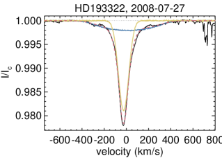
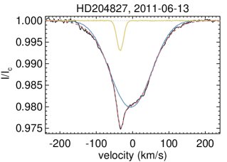
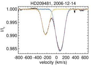
Figure 13: continued

Appendix B Assessment of LSD noise characteristics

We describe here the details of an analysis used to characterise the reliability of the LSD uncertainties. On the one hand, if the uncertainties are over-estimated this affects our ability to detect signal and therefore identify magnetic stars. On the other hand, if the uncertainties are under-estimated, this would result in a larger number of spurious detections. In order to address this problem we compared the FAPs measured from the observed null profiles to a theoretical FAP distribution, from the single star population only. The theoretical distribution was obtained by generating a series of random profiles with the same noise characteristics as the observed profiles and then measuring the FAP of each theoretical null profile. The individual pixel uncertainties used for the theoretical profiles were created assuming a Gaussian distribution with a standard deviation equal to the uncertainty found in the observed LSD profile. 100 theoretical profiles generated with random noise were obtained for each observation to create the theoretical distribution.

In Fig. 15, we compare the observed and theoretical cumulative distributions for both the binned and unbinned profiles. The obtained FAP distribution from the observed unbinned profiles is significantly different from the predicted distribution - the observed sample contains a significantly larger fraction of high-FAP values compared to the theoretical distribution. One possible interpretation of this mismatch is that the uncertainties established from the LSD procedure are incorrect. We therefore proceeded to recompute the FAP distribution by adjusting all LSD uncertainties by a fixed value. A two-sided KS test was used to find a fixed value that provided the best agreement between the noise-adjusted distribution and the predicted null distribution. The results from this exercise suggest that the LSD uncertainties are over-estimated by about 20%. We carried out this same procedure for the binned profiles and the results were very different - in this case the uncertainties were over-estimated by about 3%. We repeated this same analysis with the LSD profiles generated by the Donati et al. (1997) LSD code. The results are similar, but the LSD profiles generated with the Donati et al. code result in an over-estimation by about 10% for the unbinned profiles and 6% for the binned profiles.

Another check to test the reliability of the LSD uncertainties was to compare the mean S/N estimated from the pixel uncertainties ($1/\sigma$) with the S/N estimated from the root-mean-square (RMS) deviation from no signal in the null profiles. In the case of pure Gaussian noise, the RMS S/N should equal the $\sigma$ S/N. In Fig. 16, we compare the S/N obtained from each method. The results show that there is a systematic offset between the two S/N measurements - the S/N obtained from the RMS measurements is consistently higher than the S/N obtained from the mean uncertainty. These results are consistent with the previous analysis. Increasing the S/N measurements from the uncertainties by about 20% brings the two S/N measurements into much better agreement.

The level of disagreement of the uncertainties on the order of 10-20%, as found in this work, is consistent with other magnetometry studies (e.g. Wade et al., 2000). The unbinned profiles are used to compute $B_{\ell}$ and $N_{\ell}$ values, and so these measurements, and their uncertainties, should be considered accurate to within about 10-20%. This has little impact on the results presented in this work as the $B_{\ell}$ values are not used to establish whether a Zeeman signature is detected or not. The binned profiles are used to establish the statistical significance of a detected Zeeman signature, and, in this case, the noise characteristics of these profiles agree well with theoretical predictions.

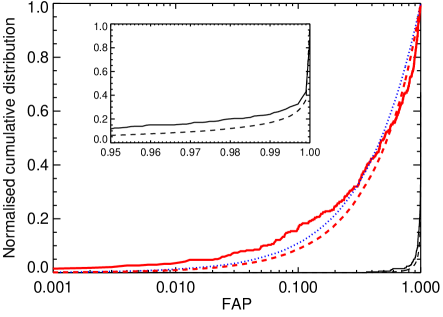
Figure 15: Comparison of cumulative distributions of the FAP. The FAP distribution obtained from the observed unbinned null profiles (thin black) and observed binned null profiles (thick red) are compared to a theoretical null distribution (dotted blue). The theoretical null distribution is the same when using the uncertainties obtained from the observed binned or unbinned profiles. Also shown are theoretical null distributions where the individual pixel uncertainties have been decreased by 20% for the unbinned profiles (thin black dashed) and decreased by 3% for the binned profiles (thick red dashed). The inset provides an expanded view of a small region of the unbinned distributions to highlight the differences. The corrected distributions significantly improve the agreement between the observed and theoretical distributions.

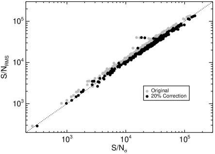
Figure 16: Comparison of the S/N level estimated from the LSD profiles ($<1/\sigma>$), versus the S/N estimated from the RMS of the diagnostic null profile. The grey points correspond to the original measurements, while the black points correspond to the same measurements, but increasing the S/N by 20%, as found from the noise analysis discussed in the text. The dotted line corresponds to a one-to-one relation.

Appendix C Summary of results

This section provides a summary of all measurements for each observation of each star. Table 5 presents the results for all presumably single O stars, while Table 14 presents the results for all stars that are either part of known multi-line spectroscopic systems, or where there is sufficient evidence to suggest that the stars are part of multi-line spectroscopic systems.

Table 5: Table of observations and magnetic results for spectroscopically single stars. Included are the names adopted in this analysis, the common name, the spectral type and the luminosity class, the adopted line mask, the observation date, the heliocentric Julian date at mid exposure (2450000+), the exposure time of the polarimetric sequence, the instrument used (ESPaDOnS (E), Narval (N), or HARPSpol (H)), the peak S/N in the co-added spectrum within the range of 500 to 600 nm, the optimal velocity width determined for the binned LSD profile, the detection flag (definite detection (DD), marginal detection (MD) or non-detection (ND)), the integration range corresponding to the line profile, the longitudinal magnetic field strength ($B_{\ell}$), the longitudinal field strength measured from the diagnostic null profile ($N_{\ell}$), and the uncertainty of the longitudinal field ($\sigma$). Also given are the results from the line fitting routine: the radial velocity ($v_{r}$), the projected rotational velocity ($v\sin i$), additional non-rotational velocity considered macroturbulence ($v_{\rm mac}$), and the median total line broadening $v_{\rm tot}$, computed by summing $v\sin i$ and $v_{\rm mac}$ in quadrature. Some observations consisted of multiple sequences with different exposure times. We list all sequences, but only provide details for the combined spectra.

Name	Common	Spec	Mask	Date	HJD	Exp	Ins	S/N	Width	Det	Int lims	$B_{\ell}$	$N_{\ell}$	$\sigma$	$v_{r}$	$v\sin i$	$v_{\rm mac}$	$v_{\rm tot}$
	name	type				(s)			(km s-1)	flag	(km s-1)	(G)	(G)	(G)	(km s-1)	(km s-1)	(km s-1)	(km s-1)
HD 108		O8f?p var	t35000g40	2007-10-15	4389.4322	$3\times 4\times 900$	N	930	16.2	ND	-300,50	-52	15	22	-95	115	98	151
				2007-10-16	4390.5286	$3\times 4\times 900$	N	831	18.0	ND	-300,50	-5	-34	27	-91	122	86	149
				2007-10-18	4392.3743	$3\times 4\times 900$	N	609	12.6	ND	-300,50	-53	13	33	-94	121	87	149
				2007-10-19	4393.4062	$3\times 4\times 900$	N	978	7.2	ND	-300,50	-61	-5	20	-93	122	96	155
				2007-10-20	4394.3890	$3\times 4\times 900$	N	958	18.0	MD	-300,50	-65	31	20	-97	124	89	153
				2007-10-21	4395.4171	$3\times 4\times 900$	N	962	14.4	MD	-300,50	-69	-9	20	-97	123	96	156
				2007-10-23	4397.3944	$3\times 4\times 900$	N	950	18.0	MD	-300,50	-36	11	21	-92	121	86	149
				2007-10-24	4398.3960	$3\times 4\times 900$	N	947	12.6	ND	-300,50	-48	-25	21	-94	119	81	144
				2008-10-14	4754.3964	$5\times 4\times 900$	N	1262	18.0	DD	-300,50	-79	-3	16	-94	119	104	158
				2008-10-15	4755.8721	$2\times 4\times 650$	E	792	16.2	ND	-300,50	-83	12	36	-98	122	93	153
				2008-10-23	4763.3783	$5\times 4\times 900$	N	1093	18.0	DD	-300,50	-107	-27	18	-95	123	90	152
				2008-10-24	4764.3587	$5\times 4\times 900$	N	1350	18.0	DD	-300,50	-54	12	15	-93	127	92	157
				2008-10-25	4765.3705	$5\times 4\times 900$	N	1013	12.6	DD	-300,50	-111	-50	18	-99	128	90	157
				2008-10-26	4766.3575	$5\times 4\times 900$	N	1058	18.0	MD	-300,50	-44	-31	18	-104	120	96	154
				2009-07-04	5018.0721	$2\times 4\times 1300$	E	1317	14.4	DD	-300,50	-97	4	17	-96	122	88	151
				2009-07-06	5020.0697	$2\times 4\times 1300$	E	1211	9.0	DD	-300,50	-151	-21	17	-97	122	86	150
				2009-07-08	5022.0717	$2\times 4\times 1300$	E	1428	12.6	DD	-300,50	-98	2	16	-98	127	72	146
				2009-07-12	5026.0672	$2\times 4\times 1300$	E	1405	18.0	MD	-300,50	-93	6	21	-101	121	95	154
				2009-07-13	5027.0801	$2\times 4\times 1300$	E	1463	18.0	ND	-300,50	-103	-11	29	-102	123	83	149
				2009-07-20	5033.5842	$3\times 4\times 750$	N	776	18.0	DD	-300,50	-125	22	28	-90	114	111	159
				2009-07-24	5037.5658	$3\times 4\times 750$	N	823	10.8	DD	-300,50	-105	-17	25	-95	131	76	151
				2009-07-25	5038.6094	$3\times 4\times 700$	N	660	12.6	ND	-300,50	-11	64	34	-94	121	98	156
				2009-07-26	5039.5963	$4\times 4\times 806$	N	745	12.6	DD	-300,50	-112	-25	29	-97	126	94	157
				2009-07-27	5040.5793	$3\times 4\times 900$	N	659	12.6	ND	-300,50	24	-30	37	-102	118	98	153
				2009-07-28	5041.5715	$3\times 4\times 900$	N	924	14.4	ND	-300,50	-44	-21	24	-99	119	86	147
				2009-07-29	5042.5830	$3\times 4\times 900$	N	1019	18.0	ND	-300,50	12	10	21	-95	125	71	144
				2009-07-30	5043.5810	$4\times 4\times 812$	N	1007	16.2	DD	-300,50	-117	6	22	-97	124	94	156
				2009-07-31	5044.5793	$3\times 4\times 812$	N	951	9.0	ND	-300,50	27	-6	24	-96	117	103	156
				2009-08-01	5045.5790	$3\times 4\times 900$	N	662	10.8	ND	-300,50	-84	-43	33	-96	124	91	154
				2009-08-03	5047.6030	$3\times 4\times 900$	N	956	16.2	DD	-300,50	-123	-19	23	-94	113	104	154
				2009-08-04	5048.5600	$3\times 4\times 900$	N	980	18.0	ND	-300,50	-80	22	22	-96	122	93	154
				2009-09-02	5078.0719	$1\times 4\times 1300$	E	874	16.2	DD	-300,50	-114	22	25	-96	118	97	153
				2009-09-07	5082.9793	$2\times 4\times 1300$	E	1373	16.2	DD	-300,50	-108	-16	19	-94	119	91	150
				2009-09-24	5099.9121	$2\times 4\times 1300$	E	1328	3.6	DD	-300,50	-138	6	15	-98	120	99	156
				2009-09-30	5105.8921	$2\times 4\times 1300$	E	1230	16.2	DD	-300,50	-95	3	18	-98	122	86	149
				2009-10-04	5109.9925	$2\times 4\times 1300$	E	851	16.2	ND	-300,50	-34	-56	79	-102	126	96	158
				2009-10-09	5114.9038	$2\times 4\times 1300$	E	1430	18.0	ND	-300,50	-151	-18	34	-98	116	106	157

Table 6: continued

Name	Common	Spec	Mask	Date	HJD	Exp	Ins	S/N	Width	Det	Int lims	$B_{\ell}$	$N_{\ell}$	$\sigma$	$v_{r}$	$v\sin i$	$v_{\rm mac}$	$v_{\rm tot}$
	name	type				(s)			(km s-1)	flag	(km s-1)	(G)	(G)	(G)	(km s-1)	(km s-1)	(km s-1)	(km s-1)
HD 13745		O9.7 II(n)	t30000g35	2012-08-21	6161.6453	$1\times 4\times 1200$	N	488	10.8	ND	-230,225	-21	60	82	-23	184	64	195
				2012-08-22	6162.6066	$1\times 4\times 1200$	N	405	16.2	ND	-230,225	-132	116	105	-20	159	112	195
				2012-08-23	6163.6452	$1\times 4\times 1200$	N	478	21.6	ND	-230,225	108	103	72	-18	179	92	201
HD 14633		ON8.5 V	t34000g40	2009-10-08	5113.8973	$1\times 4\times 1300$	E	869	19.8	ND	-230,155	-7	32	37	-35	123	86	150
HD 24431		O9 III	t32000g35	2011-11-06	5873.0370	$2\times 4\times 720$	E	1144	14.4	ND	-180,150	13	5	24	-14	58	114	128
HD 24534	X Per	O9.5npe	t32000g40	2010-12-13	5544.7754	$2\times 4\times 790$	E	1741	12.6	ND	-265,240	308	-86	111	-1	205	93	225
HD 24912	$\xi$ Per	O7.5 III(n)((f))	t35000g40	2006-12-10	4080.7723	$1\times 4\times 300$	N	2317	23.4	ND	-230,335	7	17	21	64	211	89	230
				-	-	$2\times 4\times 420$	N	-	-	-	-	-	-	-	-	-	-	-
				2006-12-13	4083.4167	$3\times 4\times 480$	N	2610	25.2	ND	-230,335	-36	28	21	69	203	85	220
				2006-12-14	4084.3789	$1\times 4\times 420$	N	2341	12.6	MD	-230,335	-43	52	22	62	217	82	232
				-	-	$2\times 4\times 480$	N	-	-	-	-	-	-	-	-	-	-	-
				2006-12-15	4085.3650	$5\times 4\times 420$	N	4324	16.2	ND	-230,335	-6	23	12	67	199	89	218
				-	-	$2\times 4\times 480$	N	-	-	-	-	-	-	-	-	-	-	-
				2006-12-16	4086.3015	$1\times 4\times 420$	N	736	18.0	ND	-230,335	93	145	77	64	219	94	238
				2007-09-06	4350.6051	$3\times 4\times 420$	N	3851	7.2	ND	-230,335	6	6	13	57	203	95	224
				-	-	$2\times 4\times 450$	N	-	-	-	-	-	-	-	-	-	-	-
				-	-	$1\times 4\times 500$	N	-	-	-	-	-	-	-	-	-	-	-
				-	-	$1\times 4\times 540$	N	-	-	-	-	-	-	-	-	-	-	-
				2007-09-07	4351.6076	$2\times 4\times 450$	N	4635	28.8	ND	-230,335	3	-1	11	52	206	109	233
				-	-	$1\times 4\times 500$	N	-	-	-	-	-	-	-	-	-	-	-
				-	-	$3\times 4\times 540$	N	-	-	-	-	-	-	-	-	-	-	-
				2007-09-08	4352.5924	$2\times 4\times 450$	N	3735	9.0	ND	-230,335	-3	16	14	54	201	87	219
				-	-	$1\times 4\times 520$	N	-	-	-	-	-	-	-	-	-	-	-
				-	-	$1\times 4\times 600$	N	-	-	-	-	-	-	-	-	-	-	-
				2007-09-09	4353.6224	$2\times 4\times 450$	N	2175	14.4	ND	-230,335	-57	15	27	59	201	106	227
				2007-09-10	4354.6398	$1\times 4\times 500$	N	1777	23.4	ND	-230,335	-26	-25	32	56	192	90	213
				2007-09-11	4355.6545	$1\times 4\times 400$	N	1668	9.0	ND	-230,335	-18	-68	34	58	207	90	225
				2007-09-12	4356.6973	$1\times 4\times 430$	N	1452	19.8	ND	-230,335	-15	64	40	56	201	95	223
				2011-10-31	5866.9213	$5\times 4\times 90$	E	2078	12.6	ND	-230,335	-20	16	27	65	187	113	218
HD 30614	$\alpha$ Cam	O9 Ia	t31000g35	2006-12-13	4083.4987	$1\times 4\times 230$	N	827	14.4	ND	-260,175	34	19	44	0	95	108	144
				2007-12-21	4456.7072	$4\times 4\times 140$	E	2854	14.4	ND	-195,175	-14	-17	12	-1	100	81	128
				2010-11-14	5516.0385	$2\times 4\times 120$	E	1487	16.2	ND	-155,175	-17	24	17	8	93	88	129
				2013-12-31	6293.8306	$1\times 4\times 140$	E	1339	14.4	ND	-235,175	34	3	29	0	99	99	140
				2012-01-01	6294.8142	$3\times 4\times 140$	E	1377	18.0	ND	-170,175	-22	40	23	14	93	96	134
HD 34078		O9.5 V	t32000g40	2007-10-15	4389.6002	$5\times 4\times 500$	N	1465	9.0	ND	-20,145	10	12	7	53	17	52	55
				2007-10-18	4392.5032	$4\times 4\times 500$	N	871	7.2	MD	-20,145	-298	110	127	53	17	55	58
				2007-10-19	4393.5066	$2\times 4\times 500$	N	1042	9.0	ND	-20,145	16	4	10	54	16	56	58
				2010-02-26	5254.7895	$1\times 4\times 200$	E	816	9.0	ND	-20,145	20	-6	13	54	14	58	60
HD 34656		O7.5 II(f)	t35000g40	2011-11-10	5877.0636	$1\times 4\times 650$	E	862	14.4	ND	-185,165	-47	-26	31	-7	70	109	130
HD 35619		O7.5 V	t36000g40	2012-01-07	5933.8654	$1\times 4\times 1300$	E	655	7.2	ND	-115,175	-10	-41	42	20	43	99	108
HD 36512	$\upsilon$ Ori	O9.7 V	t34000g45	2012-11-13	6245.5592	$1\times 4\times 360$	N	427	3.6	ND	-40,70	10	23	17	16	16	48	51
HD 36861	$\lambda$ Ori A	O8 III((f))	t34000g40	2007-12-21	4456.7322	$2\times 4\times 35$	E	1306	12.6	ND	-110,205	10	2	18	33	62	86	106
				2008-01-18	4484.8133	$1\times 4\times 35$	E	674	12.6	ND	-110,205	-8	9	36	32	63	85	106
				2008-01-22	4488.8758	$2\times 4\times 35$	E	1359	14.4	ND	-110,205	18	-16	18	33	62	87	107

Table 7: continued

Name	Common	Spec	Mask	Date	HJD	Exp	Ins	S/N	Width	Det	Int lims	$B_{\ell}$	$N_{\ell}$	$\sigma$	$v_{r}$	$v\sin i$	$v_{\rm mac}$	$v_{\rm tot}$
	name	type				(s)			(km s-1)	flag	(km s-1)	(G)	(G)	(G)	(km s-1)	(km s-1)	(km s-1)	(km s-1)
				2008-10-14	4754.5248	$2\times 4\times 90$	N	885	16.2	ND	-110,205	46	15	26	34	62	91	110
				2008-10-26	4766.4996	$7\times 4\times 90$	N	1925	9.0	ND	-110,205	-13	-26	12	35	62	89	108
				2009-03-15	4906.3005	$1\times 4\times 150$	N	975	9.0	ND	-110,205	1	48	23	32	62	88	108
				2009-03-17	4908.3350	$1\times 4\times 150$	N	1147	7.2	ND	-110,205	-20	8	20	31	62	91	110
				2010-10-16	5486.9385	$4\times 4\times 70$	E	2513	16.2	ND	-110,205	8	6	10	34	59	90	107
HD 36879		O7 V(n)((f))	t37000g40	2009-09-05	5081.0801	$1\times 4\times 900$	E	747	18.0	ND	-220,275	36	-78	78	32	187	94	209
				2012-01-31	5958.7826	$2\times 4\times 965$	E	1374	14.4	ND	-220,275	-24	-52	39	31	184	99	209
HD 38666	$\mu$ Col	O9.5 V	t32000g40	2010-01-23	5220.8493	$2\times 4\times 275$	E	1241	7.2	ND	-70,275	15	44	21	105	113	79	138
HD 42088		O6 V((f)z	t39000g40	2010-03-07	5263.8708	$1\times 4\times 580$	E	549	5.4	ND	-80,140	-13	-18	34	18	46	106	116
HD 46056		O8 Vn	t35000g40	2008-12-07	4809.1153	$2\times 4\times 877$	E	740	23.4	ND	-395,450	152	-68	181	31	349	99	363
HD 46150		O5 V((f))z	t41000g45	2007-12-22	4457.8460	$1\times 4\times 325$	E	1663	9.0	ND	-200,300	33	-32	34	41	79	176	193
				-	-	$1\times 4\times 400$	E	-	-	-	-	-	-	-	-	-	-	-
				-	-	$2\times 4\times 725$	E	-	-	-	-	-	-	-	-	-	-	-
				2008-10-17	4758.0440	$1\times 4\times 877$	E	1091	14.4	ND	-200,300	28	-61	56	45	80	179	196
				2012-01-30	5957.8122	$3\times 4\times 840$	E	2191	25.2	ND	-200,300	12	10	28	37	85	168	188
HD 46202		O9.5 V	t32000g40	2008-01-18	4484.7561	$2\times 4\times 1100$	E	616	7.2	ND	-30,100	-2	-10	13	34	21	58	62
				2012-02-01	5959.7517	$1\times 4\times 600$	E	530	5.4	ND	-30,100	-4	9	16	35	18	61	64
HD 46223		O4 V((f))	t43000g45	2007-03-07	4167.9029	$2\times 4\times 700$	E	895	14.4	ND	-160,240	80	-93	59	35	73	156	173
				2008-01-21	4487.7567	$3\times 4\times 860$	E	1409	18.0	ND	-160,240	-38	-11	35	38	73	158	174
HD 46485		O7 Vn	t37000g40	2008-12-08	4810.1209	$2\times 4\times 877$	E	496	32.4	ND	-370,410	187	-269	418	18	318	180	366
				2008-12-09	4811.1389	$2\times 4\times 877$	E	739	36.0	ND	-370,410	169	165	117	29	316	109	334
				2012-02-13	5971.7504	$1\times 4\times 1740$	E	880	37.8	ND	-370,410	45	-103	121	31	314	107	332
HD 46966		O8.5 IV	t32000g35	2012-02-01	5959.9724	$1\times 4\times 1040$	E	1179	10.8	ND	-70,150	-4	-13	16	34	50	90	102
HD 47432	V689 Mon	O9.7 Ib	t30000g35	2012-02-01	5959.9033	$1\times 4\times 720$	E	1303	12.6	ND	-115,225	-3	-10	19	59	93	94	132
HD 55879		O9.7 III	t31000g35	2008-08-20	4760.1195	$1\times 4\times 600$	E	1368	14.4	ND	-115,175	-4	-15	15	28	36	77	85
HD 57682		O9.5 IV	t32000g40	2008-12-04	4806.0799	$1\times 4\times 500$	E	302	9.0	MD	-60,110	255	18	55	21	8	65	65
				2008-12-05	4807.1081	$1\times 4\times 500$	E	922	1.8	DD	-60,110	137	20	15	22	4	61	61
				2009-05-03	4955.7675	$2\times 4\times 600$	E	1418	9.0	DD	-60,110	-40	8	11	23	14	63	64
				2009-05-04	4956.7498	$2\times 4\times 540$	E	1346	9.0	DD	-60,110	-39	-15	12	22	14	64	65
				2009-05-06	4958.7805	$1\times 4\times 540$	E	633	9.0	MD	-60,110	-42	-1	23	23	10	72	73
				2009-05-07	4959.7489	$2\times 4\times 540$	E	1060	3.6	DD	-60,110	-74	6	14	22	16	66	68
				2009-05-08	4960.7480	$2\times 4\times 540$	E	873	5.4	DD	-60,110	-110	11	17	22	10	72	72
				2009-12-30	5197.0958	$2\times 4\times 540$	E	1529	1.8	DD	-60,110	144	3	10	23	6	54	54
				2010-01-03	5201.0428	$2\times 4\times 540$	E	1106	1.8	DD	-60,110	101	-32	12	24	0	62	62
				2010-01-22	5219.9545	$2\times 4\times 540$	E	1338	1.8	DD	-60,110	-121	0	12	22	16	60	62
				2010-01-28	5225.9836	$2\times 4\times 540$	E	1571	1.8	DD	-60,110	-120	-19	11	22	16	58	60
				2010-01-30	5228.0016	$2\times 4\times 540$	E	1164	1.8	DD	-60,110	-114	22	13	22	15	62	63
				2010-01-31	5228.9032	$2\times 4\times 540$	E	1217	1.8	DD	-60,110	-92	-4	19	22	15	62	64
				2010-02-23	5251.9132	$2\times 4\times 414$	E	1170	1.8	DD	-60,110	154	-9	12	22	3	55	55
				2010-02-27	5255.9891	$2\times 4\times 414$	E	909	1.8	DD	-60,110	177	13	18	22	8	60	60
				2010-03-03	5259.9420	$2\times 4\times 414$	E	1134	1.8	DD	-60,110	152	0	13	21	12	52	54
				2010-03-07	5263.9096	$2\times 4\times 414$	E	859	1.8	DD	-60,110	98	-19	14	22	9	62	63
				2010-11-27	5529.0352	$2\times 4\times 415$	E	1178	9.0	DD	-60,110	-57	19	13	23	18	61	64
				2010-12-23	5555.0640	$2\times 4\times 415$	E	1040	9.0	MD	-60,110	0	3	14	22	8	66	66

Table 8: continued

Name	Common	Spec	Mask	Date	HJD	Exp	Ins	S/N	Width	Det	Int lims	$B_{\ell}$	$N_{\ell}$	$\sigma$	$v_{r}$	$v\sin i$	$v_{\rm mac}$	$v_{\rm tot}$
	name	type				(s)			(km s-1)	flag	(km s-1)	(G)	(G)	(G)	(km s-1)	(km s-1)	(km s-1)	(km s-1)
				2010-12-30	5561.0732	$2\times 4\times 415$	E	957	1.8	DD	-60,110	92	-6	14	22	5	62	62
HD 66788		O8 V	t35000g40	2010-01-23	5220.9878	$1\times 4\times 600$	E	189	14.4	ND	15,280	53	-122	90	149	27	87	91
				2010-01-31	5228.9922	$1\times 4\times 600$	E	219	9.0	ND	15,280	-179	-74	114	148	27	83	88
HD 66811	$\zeta$ Pup	O4 If	t40000g40	2011-12-13	5909.7247	$5\times 4\times 120$	H	1940	18.0	MD	-345,300	27	-51	22	-16	175	198	264
				2012-02-13	5971.8333	$30\times 4\times 20$	E	6195	32.4	ND	-345,300	-5	-2	15	-14	200	158	255
HD 69106		O9.7 In	t30000g35	2012-01-09	5937.0428	$1\times 4\times 1710$	E	1183	27.0	ND	-340,375	113	255	92	10	311	81	321
HD 93028		O9 IV	t32000g40	2013-02-17	6341.6832	$2\times 4\times 700$	H	179	5.4	ND	-65,120	42	-13	42	27	29	81	86
HD 148937		O6f?p	t38000g40	2009-05-02	4955.0466	$1\times 4\times 680$	E	976	10.8	ND	-165,100	-39	131	58	-56	76	126	148
				2009-05-07	4959.9732	$1\times 4\times 680$	E	529	5.4	ND	-165,100	-317	86	105	-59	66	157	171
				2009-09-03	5078.7452	$2\times 4\times 600$	E	733	9.0	ND	-165,100	-97	119	77	-58	71	151	167
				2010-06-18	5366.8954	$2\times 4\times 600$	E	1161	12.6	MD	-165,100	-158	-71	39	-48	75	136	155
				2010-06-19	5367.9025	$2\times 4\times 600$	E	1157	14.4	MD	-165,100	-187	-7	45	-52	64	135	149
				2010-06-20	5368.8751	$2\times 4\times 600$	E	1074	14.4	MD	-165,100	-100	16	47	-50	70	127	145
				2010-06-21	5369.9019	$2\times 4\times 600$	E	752	14.4	MD	-165,100	-208	4	74	-54	71	127	146
				2010-06-22	5370.8613	$2\times 4\times 600$	E	630	12.6	ND	-165,100	-43	247	82	-54	59	138	150
				2010-06-23	5371.8590	$2\times 4\times 600$	E	1187	7.2	MD	-165,100	-116	-8	43	-51	73	121	141
				2010-06-24	5372.8647	$2\times 4\times 600$	E	1138	12.6	DD	-165,100	-85	33	39	-52	73	130	149
				2010-07-22	5400.7887	$2\times 4\times 600$	E	1036	12.6	ND	-165,100	-44	-13	51	-53	71	131	149
				2010-07-23	5401.7989	$2\times 4\times 600$	E	232	14.4	ND	-165,100	90	202	403	-53	57	152	162
				2010-07-24	5402.7923	$2\times 4\times 600$	E	427	14.4	ND	-165,100	-13	103	138	-55	74	131	151
				2010-07-25	5403.7958	$2\times 4\times 600$	E	890	7.2	ND	-165,100	23	-34	63	-56	73	130	149
				2010-07-26	5404.8023	$2\times 4\times 600$	E	1066	9.0	ND	-165,100	23	18	51	-54	69	129	146
				2010-07-27	5405.7784	$2\times 4\times 600$	E	1213	14.4	ND	-165,100	19	35	44	-53	76	120	142
				2010-07-28	5406.7679	$2\times 4\times 600$	E	1201	10.8	MD	-165,100	59	-77	43	-53	78	126	148
HD 149038	$\mu$ Nor	O9.7 Iab	t30000g35	2010-07-30	5408.7713	$3\times 4\times 250$	E	2029	7.2	ND	-116,160	-1	7	11	8	67	102	122
HD 149757	$\zeta$ Oph	O9.5 Ivnn	t30000g35	2011-03-18	5639.7152	$1\times 4\times 45$	N	814	30.6	ND	-420,420	-146	-185	160	-5	353	114	371
				2011-03-21	5642.6222	$1\times 4\times 45$	N	842	39.6	ND	-420,420	154	64	150	0	362	83	372
				2011-04-05	5657.6642	$1\times 4\times 45$	N	874	18.0	ND	-420,420	-289	-85	145	0	351	97	364
				2011-05-17	5699.4867	$1\times 4\times 45$	N	922	25.2	ND	-420,420	-367	162	142	-1	370	49	373
				2011-06-08	5721.9033	$20\times 4\times 45$	E	2621	32.4	ND	-420,420	54	3	49	0	353	117	372
				2011-06-10	5723.5012	$1\times 4\times 45$	N	861	37.8	ND	-420,420	-69	-70	171	1	356	112	373
				2011-06-13	5726.4798	$1\times 4\times 45$	N	739	18.0	ND	-420,420	17	110	169	-1	365	103	379
				2011-06-14	5727.4664	$1\times 4\times 45$	N	1004	41.4	ND	-420,420	8	-54	123	0	367	124	387
				2011-06-15	5728.4821	$1\times 4\times 45$	N	847	32.4	ND	-420,420	57	146	152	-4	362	110	378
				2011-07-04	5747.4769	$1\times 4\times 45$	N	1000	9.0	ND	-420,420	-33	55	126	0	360	84	370
				2011-07-07	5750.4789	$1\times 4\times 45$	N	747	41.4	ND	-420,420	-55	-130	169	0	368	88	379
				2011-07-10	5753.4412	$1\times 4\times 45$	N	940	23.4	ND	-420,420	149	-67	138	2	368	53	372
				2011-07-11	5754.4292	$1\times 4\times 45$	N	955	18.0	ND	-420,420	33	136	126	1	355	167	393
				2011-08-10	5784.3431	$1\times 4\times 45$	N	953	30.6	ND	-420,420	-134	-247	129	0	342	192	392
				2011-08-11	5785.3411	$1\times 4\times 45$	N	875	12.6	ND	-420,420	-195	-68	140	1	356	147	386
				2011-08-15	5789.3449	$1\times 4\times 45$	N	828	37.8	ND	-420,420	-203	-113	150	-2	358	106	373
				2011-08-16	5790.3385	$1\times 4\times 45$	N	892	27.0	ND	-420,420	-140	-34	136	1	360	144	388
				2011-08-17	5791.3380	$1\times 4\times 45$	N	892	32.4	ND	-420,420	62	-20	138	-1	363	133	387
				2011-08-18	5792.4038	$1\times 4\times 45$	N	551	39.6	ND	-420,420	61	-202	207	2	362	163	397

Table 9: continued

Name	Common	Spec	Mask	Date	HJD	Exp	Ins	S/N	Width	Det	Int lims	$B_{\ell}$	$N_{\ell}$	$\sigma$	$v_{r}$	$v\sin i$	$v_{\rm mac}$	$v_{\rm tot}$
	name	type				(s)			(km s-1)	flag	(km s-1)	(G)	(G)	(G)	(km s-1)	(km s-1)	(km s-1)	(km s-1)
				2011-08-20	5794.4007	$1\times 4\times 45$	N	751	34.2	ND	-420,420	181	-197	155	0	375	97	388
				2011-08-21	5795.3316	$1\times 4\times 45$	N	1021	30.6	ND	-420,420	143	110	122	3	351	157	385
				2011-08-22	5796.3507	$1\times 4\times 45$	N	634	36.0	ND	-420,420	146	-235	198	-1	373	78	381
				2011-08-23	5797.3309	$1\times 4\times 45$	N	1051	5.4	ND	-420,420	-63	40	120	-1	367	91	378
				2011-08-26	5800.3249	$1\times 4\times 45$	N	517	28.8	ND	-420,420	1	-137	266	2	363	129	386
				2011-08-27	5801.3478	$1\times 4\times 45$	N	593	30.6	ND	-420,420	193	131	205	-1	363	130	386
				2011-08-28	5802.3253	$1\times 4\times 45$	N	556	27.0	ND	-420,420	-94	350	302	0	368	128	390
				2012-01-16	5943.7772	$1\times 4\times 45$	N	718	7.2	ND	-420,420	142	166	172	-6	372	69	378
				2012-01-17	5944.7437	$1\times 4\times 45$	N	807	43.2	ND	-420,420	163	9	155	-1	370	78	378
				2012-01-24	5951.7745	$1\times 4\times 45$	N	1001	18.0	ND	-420,420	-14	32	129	0	349	131	373
				2012-01-25	5952.7690	$1\times 4\times 45$	N	1134	30.6	ND	-420,420	2	85	110	0	359	125	380
				2012-01-27	5954.7475	$1\times 4\times 45$	N	537	34.2	ND	-420,420	90	133	232	1	368	85	377
				2012-06-21	6100.3841	$1\times 4\times 45$	N	881	9.0	ND	-420,420	22	5	141	1	341	208	400
				2012-06-22	6101.3752	$1\times 4\times 45$	N	950	43.2	ND	-420,420	-75	-175	131	0	354	147	383
				2012-06-23	6102.4691	$1\times 4\times 45$	N	1015	10.8	ND	-420,420	-9	-205	117	1	370	163	404
				2012-07-09	6118.3834	$1\times 4\times 45$	N	907	10.8	ND	-420,420	-114	293	137	0	358	115	376
				2012-07-12	6121.3793	$1\times 4\times 45$	N	844	36.0	ND	-420,420	-54	121	142	1	378	121	397
				2012-08-06	6146.3435	$1\times 4\times 45$	N	968	37.8	ND	-420,420	179	30	128	1	367	101	380
				2012-08-07	6147.3406	$1\times 4\times 45$	N	790	21.6	ND	-420,420	64	-219	156	-3	365	62	370
				2012-08-08	6148.3422	$1\times 4\times 45$	N	913	32.4	ND	-420,420	107	-184	137	1	364	91	375
				2012-08-09	6149.3421	$1\times 4\times 45$	N	743	39.6	ND	-420,420	-342	79	161	-1	353	202	407
				2012-08-12	6152.3450	$1\times 4\times 45$	N	624	16.2	ND	-420,420	-46	282	196	0	358	83	368
				2012-08-14	6154.3514	$1\times 4\times 45$	N	858	28.8	ND	-420,420	-203	-143	146	0	364	155	396
				2012-08-16	6156.3397	$1\times 4\times 45$	N	649	34.2	ND	-420,420	-55	-55	182	1	358	91	369
				2012-08-17	6157.3362	$1\times 4\times 45$	N	741	14.4	ND	-420,420	22	-1	163	1	376	61	381
				2012-08-18	6158.3456	$1\times 4\times 45$	N	687	39.6	ND	-420,420	207	277	176	0	371	99	384
				2012-08-19	6159.3486	$1\times 4\times 45$	N	767	10.8	ND	-420,420	-115	162	156	1	347	201	401
				2012-08-20	6160.3356	$1\times 4\times 45$	N	789	19.8	ND	-420,420	351	174	156	1	358	102	372
HD 151804	V973 Sco	O8 Iaf	t33000g40	2011-05-26	5708.8607	$2\times 4\times 800$	H	693	9.0	ND	-200,80	-19	-12	26	-56	79	86	116
HD 152233		O6 III(f)	t38000g40	2011-07-09	5752.8627	$1\times 4\times 1035$	E	1320	19.8	ND	-235,143	-65	22	36	-39	87	141	166
HD 152247		O9.5 II-III	t31000g35	2011-07-06	5749.8714	$1\times 4\times 815$	E	378	18.0	ND	-203,172	-63	67	87	-28	77	132	153
HD 152249		OC9 Iab	t30000g35	2011-07-13	5756.8794	$1\times 4\times 925$	E	1238	19.8	ND	-222,157	56	32	27	-26	82	104	132
HD 152408	HR 6272	O8 Iafpe	t32000g35	2012-07-05	6114.8740	$3\times 4\times 500$	E	1545	10.8	ND	-270,45	13	-50	42	-95	78	157	175
HD 153919		O6 Iaf	t35000g40	2011-06-13	5726.9951	$1\times 4\times 625$	E	987	12.6	ND	-330,130	70	-23	73	-91	121	162	203
HD 154368	V1074 Sco	O9.5 Iab	t30000g35	2011-03-15	5637.0916	$1\times 4\times 700$	E	1269	12.6	ND	-110,155	10	12	14	12	74	98	123
HD 154643		O9.5 III	t31000g35	2011-07-01	5744.8787	$1\times 4\times 1340$	E	1113	9.0	ND	-140,180	-13	13	23	17	106	87	137
HD 155806		O7.5 V	t36000g40	2008-06-24	4642.9151	$10\times 4\times 300$	E	3070	9.0	ND	-125,150	-45	9	14	8	71	109	130
				2008-07-19	4667.8746	$5\times 4\times 300$	E	1592	14.4	ND	-125,150	-12	-7	26	12	69	127	144
				2008-07-25	4673.8225	$5\times 4\times 300$	E	2092	14.4	ND	-125,150	-8	-9	16	10	67	137	153
				2008-07-26	4674.8225	$5\times 4\times 300$	E	2092	14.4	ND	-125,150	4	-12	15	10	65	143	157
HD 156154		O7.5 Ibf	t33000g40	2012-06-22	6101.9297	$1\times 4\times 940$	E	711	16.2	ND	-155,170	-23	-21	41	-1	80	108	134
HD 162978	63 Oph	O8 II(f)	t35000g40	2008-07-28	4676.8010	$1\times 4\times 700$	E	1268	19.8	MD	-200,180	111	12	23	-10	81	112	138
				2012-06-21	6100.9532	$4\times 4\times 720$	E	2329	18.0	ND	-200,180	-12	-9	14	-12	76	110	133
HD 164492		O7.5 Vz	t35000g40	2011-06-13	5727.0256	$1\times 4\times 430$	E	465	10.8	ND	-100,110	74	-1	35	-5	37	86	94

Table 10: continued

Name	Common	Spec	Mask	Date	HJD	Exp	Ins	S/N	Width	Det	Int lims	$B_{\ell}$	$N_{\ell}$	$\sigma$	$v_{r}$	$v\sin i$	$v_{\rm mac}$	$v_{\rm tot}$
	name	type				(s)			(km s-1)	flag	(km s-1)	(G)	(G)	(G)	(km s-1)	(km s-1)	(km s-1)	(km s-1)
HD 167263	16 Sgr	O9.5 II-IIIn	t31000g35	2011-06-14	5728.0772	$1\times 4\times 500$	E	1200	25.2	ND	-230,258	-74	-39	44	5	51	201	207
HD 167264	15 Sgr	O9.7 Iab	t30000g35	2005-06-20	3543.0215	$3\times 4\times 300$	E	1263	5.4	ND	-155,170	-14	-3	19	19	78	92	120
				2009-07-25	5038.3841	$1\times 4\times 675$	N	917	12.6	ND	-155,170	1	-8	26	-1	60	104	120
				2009-07-26	5039.3971	$1\times 4\times 600$	N	539	16.2	ND	-155,170	4	-19	43	0	1	141	141
				2009-07-27	5040.3804	$1\times 4\times 600$	N	788	10.8	ND	-155,170	-4	-8	30	-1	62	102	119
				2009-07-28	5041.3726	$1\times 4\times 600$	N	943	12.6	ND	-155,170	-17	25	24	0	61	101	118
				2009-07-29	5042.3784	$1\times 4\times 600$	N	1039	18.0	ND	-155,170	13	-30	23	1	47	112	121
				2009-07-31	5044.3835	$1\times 4\times 575$	N	980	16.2	ND	-155,170	-9	23	23	0	59	112	127
				2009-08-04	5048.4338	$1\times 4\times 575$	N	841	18.0	DD	-155,170	58	-16	28	0	34	134	139
				2011-06-18	5732.0087	$5\times 4\times 350$	E	584	14.4	ND	-155,170	106	-61	53	0	58	108	123
HD 186980		O7.5 III((f))	t35000g40	2010-06-03	5352.0394	$1\times 4\times 1300$	E	963	9.0	ND	-135,150	12	4	19	0	69	102	123
HD 188001	9 Sge	O7.5 Iabf	t34000g40	2010-07-23	5401.0197	$1\times 4\times 720$	E	666	18.0	ND	-145,190	-5	-24	42	2	84	120	147
HD 188209		O9.5 Iab	t30000g35	2008-06-21	4639.4823	$3\times 4\times 675$	N	1065	10.8	ND	-180,160	-42	6	22	-8	69	92	115
				2008-06-22	4640.4853	$3\times 4\times 675$	N	1907	9.0	ND	-180,160	-14	9	13	-13	66	96	116
				2008-06-25	4643.4814	$5\times 4\times 675$	N	2244	9.0	ND	-180,160	-11	-18	10	-5	75	92	118
				2008-06-27	4645.4606	$5\times 4\times 675$	N	2626	12.6	ND	-180,160	-3	-4	9	-14	73	108	131
				2008-06-28	4646.4620	$5\times 4\times 675$	N	3365	18.0	ND	-180,160	-17	2	10	-7	65	105	123
				2008-06-29	4647.6248	$3\times 4\times 675$	N	1925	12.6	ND	-180,160	24	-21	12	-13	70	93	116
				2008-06-30	4648.4493	$3\times 4\times 675$	N	1536	16.2	ND	-180,160	-5	-18	13	-7	71	93	117
				2010-06-24	5373.0832	$1\times 4\times 400$	E	1243	18.0	ND	-180,160	-19	6	20	-10	76	95	122
HD 189957		O9.7 III	t31000g35	2008-10-15	4755.7132	$1\times 4\times 860$	E	656	10.8	ND	-100,185	-70	63	33	34	84	90	122
HD 192281	V2011 Cyg	O4.5 Vn(f)	t42000g45	2012-08-13	6153.4443	$1\times 4\times 1500$	N	482	28.8	ND	-300,320	-330	51	156	-30	254	218	334
				2012-08-14	6154.4049	$1\times 4\times 1500$	N	530	10.8	ND	-300,320	-74	281	139	-27	256	219	337
HD 192639		O7.5 Iabf	t34000g40	2012-08-08	6148.5135	$1\times 4\times 1800$	N	802	18.0	ND	-170,170	-63	27	34	1	93	119	151
HD 201345		ON9.5 IV	t30000g35	2010-07-25	5404.0871	$1\times 4\times 700$	E	346	9.0	ND	-125,170	-57	0	65	17	91	91	129
HD 203064	68 Cyg	O7.5 IIIn((f))	t35000g40	2006-12-16	4086.3320	$1\times 4\times 540$	N	705	21.6	ND	-325,370	145	-146	263	25	287	88	300
				2007-09-10	4354.5400	$1\times 4\times 600$	N	1322	30.6	ND	-340,390	87	-131	59	8	286	93	300
				2007-11-12	4417.2759	$1\times 4\times 200$	N	737	37.8	ND	-325,420	-26	-35	110	45	285	103	303
				2012-09-29	6200.8041	$5\times 4\times 245$	E	3158	36.0	ND	-315,400	3	-30	26	30	289	95	304
HD 206183		O9.5 IV-V	t30000g35	2010-07-23	5400.9447	$1\times 4\times 250$	E	376	3.6	ND	-60,35	-7	8	17	-14	14	39	42
HD 207198		O9 II	t32000g35	2009-07-24	5037.4429	$1\times 4\times 675$	N	722	10.8	ND	-155,130	-44	-11	23	-17	67	111	130
				2009-07-25	5038.4357	$2\times 4\times 675$	N	1104	5.4	ND	-155,130	-9	18	15	-18	70	109	129
				2009-07-27	5040.4339	$2\times 4\times 675$	N	864	12.6	ND	-155,130	13	17	19	-18	72	104	126
				2009-07-28	5041.4247	$2\times 4\times 675$	N	1258	14.4	ND	-155,130	1	-18	13	-19	71	110	131
				2009-07-29	5042.4406	$2\times 4\times 675$	N	1320	9.0	ND	-155,130	2	21	13	-21	69	100	122
				2009-07-30	5043.4198	$2\times 4\times 675$	N	1257	9.0	ND	-155,130	30	-4	13	-24	70	98	120
				2009-07-31	5044.4381	$2\times 4\times 675$	N	1359	7.2	ND	-155,130	-17	4	12	-18	68	104	124
				2009-08-01	5045.4408	$1\times 4\times 675$	N	899	5.4	ND	-155,130	35	8	27	-20	70	105	126
				2009-08-04	5048.4691	$1\times 4\times 675$	N	901	14.4	ND	-155,130	-14	9	19	-23	71	101	123
				2010-07-25	5404.1181	$1\times 4\times 600$	E	850	14.4	ND	-155,130	-33	21	25	-23	68	106	126
HD 207538		O9.7 IV	t30000g35	2008-07-30	4677.9267	$1\times 4\times 1000$	E	793	7.2	ND	-100,70	-5	-12	13	-18	33	72	79
HD 209975	19 Cep	O9 Ib	t31000g35	2006-12-13	4083.2886	$1\times 4\times 660$	N	1093	16.2	ND	-175,170	-26	10	23	-17	71	101	124

Table 11: continued

Name	Common	Spec	Mask	Date	HJD	Exp	Ins	S/N	Width	Det	Int lims	$B_{\ell}$	$N_{\ell}$	$\sigma$	$v_{r}$	$v\sin i$	$v_{\rm mac}$	$v_{\rm tot}$
	name	type				(s)			(km s-1)	flag	(km s-1)	(G)	(G)	(G)	(km s-1)	(km s-1)	(km s-1)	(km s-1)
				2007-11-09	4414.4893	$1\times 4\times 550$	N	787	16.2	ND	-175,170	27	-26	31	-17	69	106	126
				2007-11-13	4418.2738	$1\times 4\times 200$	N	459	16.2	ND	-175,170	-94	25	51	-17	73	112	134
				2007-12-21	4639.5936	$3\times 4\times 275$	E	2157	18.0	ND	-175,170	-25	5	11	-17	74	104	128
				2008-06-21	4639.5936	$5\times 4\times 450$	N	1572	7.2	ND	-175,170	19	-25	14	-9	84	105	134
				2008-06-22	4640.5958	$5\times 4\times 450$	N	2341	14.4	ND	-175,170	16	-13	10	-15	65	108	126
				2008-06-25	4643.6168	$3\times 4\times 450$	N	2029	14.4	ND	-175,170	9	-28	12	-15	72	100	123
				2008-06-27	4645.6138	$5\times 4\times 450$	N	2942	12.6	ND	-175,170	24	0	8	-17	63	104	122
				2008-06-28	4645.6138	$5\times 4\times 450$	N	2527	18.0	DD	-175,170	-7	-9	8	-18	61	110	125
				2010-07-26	4646.6087	$4\times 4\times 250$	E	1313	3.6	ND	-175,170	-13	14	19	-17	71	112	133
HD 210809		O9 Iab	t31000g35	2011-06-19	5733.0596	$1\times 4\times 1100$	E	963	16.2	ND	-225,90	-5	-9	23	-75	94	105	140
HD 210839	$\lambda$ Cep	O6.5 I(n)fp	t35000g40	2006-12-13	4083.3250	$1\times 4\times 660$	N	1039	10.8	ND	-330,240	-43	-24	60	-74	215	98	236
				2011-07-07	5750.5962	$1\times 4\times 660$	N	1225	16.2	ND	-330,240	23	-107	53	-69	197	121	231
				2011-07-08	5751.6033	$1\times 4\times 660$	N	1289	23.4	ND	-330,240	-75	-83	53	-67	195	88	214
				2011-08-10	5784.5415	$1\times 4\times 660$	N	1312	28.8	ND	-330,240	42	13	50	-59	209	109	235
				2011-08-27	5801.5608	$1\times 4\times 660$	N	991	10.8	ND	-330,240	-34	-47	65	-63	200	122	235
				2011-08-28	5802.5492	$1\times 4\times 660$	N	1330	23.4	ND	-330,240	34	-20	54	-59	208	108	235
				2012-06-16	6095.6192	$1\times 4\times 660$	N	803	9.0	ND	-330,240	15	65	81	-67	180	108	210
				2012-06-22	6101.6012	$1\times 4\times 660$	N	1246	25.2	ND	-330,240	-18	-60	58	-69	203	101	227
				2012-06-24	6103.5574	$1\times 4\times 660$	N	910	21.6	ND	-330,240	60	29	75	-70	195	124	232
				2012-07-09	6118.5796	$1\times 4\times 660$	N	1074	16.2	ND	-330,240	190	-13	65	-61	179	145	231
				2012-07-18	6127.6186	$1\times 4\times 660$	N	1284	25.2	ND	-330,240	-134	40	53	-70	218	98	239
				2012-07-19	6128.6044	$1\times 4\times 660$	N	1224	14.4	ND	-330,240	-24	73	58	-64	199	125	235
				2012-07-22	6131.5983	$1\times 4\times 660$	N	1293	23.4	ND	-330,240	102	14	58	-66	165	148	222
				2012-07-23	6132.5925	$1\times 4\times 660$	N	1242	21.6	ND	-330,240	-11	-117	52	-60	216	87	233
				2012-07-24	6133.6173	$1\times 4\times 660$	N	1339	27.0	ND	-330,240	-2	-74	51	-65	191	115	223
				2012-08-06	6146.5919	$1\times 4\times 660$	N	1422	28.8	ND	-330,240	-57	-68	45	-67	169	158	231
				2012-08-07	6147.5646	$1\times 4\times 660$	N	1076	28.8	ND	-330,240	35	36	69	-78	200	108	227
				2012-08-08	6148.5762	$1\times 4\times 660$	N	1229	16.2	ND	-330,240	72	28	60	-59	198	91	218
				2012-08-09	6149.5869	$1\times 4\times 660$	N	1373	23.4	ND	-330,240	-43	-2	49	-68	189	131	230
				2012-08-11	6151.5983	$1\times 4\times 660$	N	882	28.8	ND	-330,240	164	-177	105	-70	206	100	229
				2012-08-12	6152.5376	$1\times 4\times 660$	N	772	14.4	ND	-330,240	-113	175	85	-62	186	116	220
				2012-08-13	6153.5309	$1\times 4\times 660$	N	1307	27.0	ND	-330,240	76	-68	59	-74	200	116	231
				2012-08-15	6155.5435	$1\times 4\times 660$	N	848	12.6	ND	-330,240	38	1	76	-57	195	129	234
				2012-08-16	6156.5190	$1\times 4\times 660$	N	1003	27.0	ND	-330,240	4	-6	68	-57	204	89	222
				2012-08-17	6157.5429	$1\times 4\times 660$	N	1014	21.6	ND	-330,240	-109	80	70	-60	214	95	234
				2012-08-18	6158.6321	$1\times 4\times 660$	N	720	19.8	ND	-330,240	-129	110	128	-75	199	105	226
HD 214680	10 Lac	O9 V	t33000g40	2006-12-10	4080.2870	$1\times 4\times 600$	N	1276	3.6	ND	-105,85	-3	-6	11	-11	29	43	52
				2006-12-11	4081.2425	$1\times 4\times 600$	N	1314	9.0	ND	-105,85	-8	1	11	-10	27	45	53
				2006-12-13	4083.2366	$1\times 4\times 150$	N	-	7.2	ND	-105,85	-5	-3	12	-10	25	49	55
				2006-12-14	4084.2390	$1\times 4\times 600$	N	1241	10.8	ND	-105,85	-10	-15	11	-11	27	46	53
				2006-12-15	4085.2358	$1\times 4\times 600$	N	1406	10.8	ND	-105,85	-12	5	11	-11	27	44	52
				2006-12-16	4086.2369	$1\times 4\times 600$	N	1168	10.8	ND	-105,85	-8	8	14	-10	26	48	54
				2007-09-07	4351.4938	$1\times 4\times 600$	N	1382	10.8	ND	-105,85	3	3	11	-10	25	46	53

Table 12: continued

Name	Common	Spec	Mask	Date	HJD	Exp	Ins	S/N	Width	Det	Int lims	$B_{\ell}$	$N_{\ell}$	$\sigma$	$v_{r}$	$v\sin i$	$v_{\rm mac}$	$v_{\rm tot}$
	name	type				(s)			(km s-1)	flag	(km s-1)	(G)	(G)	(G)	(km s-1)	(km s-1)	(km s-1)	(km s-1)
				2007-10-15	4389.3354	$3\times 4\times 300$	N	1596	10.8	ND	-105,85	17	3	9	-11	27	43	51
				2007-10-16	4390.4334	$3\times 4\times 300$	N	1377	10.8	ND	-105,85	-11	9	10	-9	26	46	53
				2007-10-17	4391.4930	$3\times 4\times 500$	N	2188	9.0	ND	-105,85	-3	-5	7	-11	25	45	52
				2007-10-18	4392.2742	$3\times 4\times 300$	N	1139	9.0	ND	-105,85	11	1	12	-10	27	47	54
				2007-10-19	4393.2939	$3\times 4\times 500$	N	1993	5.4	ND	-105,85	9	-1	7	-9	25	45	52
				2007-10-20	4394.2781	$3\times 4\times 500$	N	2022	5.4	ND	-105,85	9	6	7	-11	28	42	50
				2007-10-21	4395.2927	$3\times 4\times 500$	N	1781	7.2	ND	-105,85	-10	10	8	-10	29	39	49
				2007-10-23	4397.2818	$3\times 4\times 500$	N	1892	10.8	ND	-105,85	-1	8	8	-11	28	42	50
				2007-10-24	4398.2859	$3\times 4\times 500$	N	2113	7.2	ND	-105,85	5	-11	7	-10	25	44	51
				2007-11-06	4411.4652	$1\times 4\times 200$	N	622	9.0	ND	-105,85	10	-10	21	-10	26	51	57
				2008-07-26	4675.0209	$1\times 4\times 100$	E	895	7.2	ND	-105,85	-26	18	15	-10	24	53	58
HD 218195		O8.5 III	t33000g40	2011-07-04	5733.1055	$1\times 4\times 1200$	E	675	10.8	ND	-145,105	-30	27	25	-29	62	88	108
HD 218915		O9.5 Iab	t30000g35	2011-06-19	5733.1055	$1\times 4\times 1200$	E	977	5.4	ND	-200,35	22	2	17	-88	66	94	114
HD 227757		O9.5 V	t32000g40	2010-06-24	5373.0974	$1\times 4\times 30$	E	52	5.4	ND	-80,35	-13	125	227	-31	24	50	55
				2010-07-25	5404.0568	$1\times 4\times 290$	E	137	7.2	ND	-80,35	7	47	59	-30	25	51	57
HD 258691		O9.5 IV	t33000g40	2008-01-22	4488.7572	$3\times 4\times 860$	E	441	7.2	ND	-70,145	-52	4	36	35	23	75	78
HD 328856		O9.7 II	t31000g35	2012-07-06	6115.8643	$1\times 4\times 1635$	E	717	18.0	ND	-200,140	85	-42	49	-32	98	118	153
BD+60 499		O9.5 V	t32000g40	2008-08-18	4698.0339	$1\times 4\times 800$	E	199	7.2	ND	-110,20	-5	6	45	-46	26	51	57
CPD-28 2561	CD-28 5104	O6.5f?p	t32000g40	2009-01-12	4845.0187	$2\times 4\times 1085$	E	320	19.8	ND	-110,340	200	91	235	79	84	166	186
				2011-12-09	5905.7982	$2\times 4\times 900$	H	111	18.0	ND	-110,340	131	1407	569	47	82	152	173
				2012-01-03	5931.0435	$2\times 4\times 1085$	E	398	18.0	ND	-110,340	-603	-313	326	82	6	199	199
				2012-01-04	5931.8858	$2\times 4\times 1085$	E	382	14.4	ND	-110,340	-838	-634	375	76	3	200	200
				2012-01-05	5933.0340	$1\times 4\times 1085$	E	263	12.6	ND	-110,340	-101	-535	594	73	5	195	195
				2012-01-06	5934.0025	$1\times 4\times 1085$	E	247	23.4	ND	-110,340	-1751	-431	664	72	5	197	197
				2012-01-07	5934.9999	$1\times 4\times 1085$	E	308	21.6	ND	-110,340	-353	184	461	74	4	202	202
				2012-01-08	5936.0127	$1\times 4\times 1085$	E	284	7.2	ND	-110,340	-707	284	483	79	4	198	198
				2012-01-09	5936.9512	$1\times 4\times 1085$	E	279	21.6	ND	-110,340	-719	-1154	472	84	20	201	202
				2012-01-11	5938.9264	$1\times 4\times 1085$	E	291	23.4	ND	-110,340	-268	-109	393	87	35	200	203
				2012-01-13	5940.9614	$1\times 4\times 1085$	E	222	18.0	ND	-110,340	43	761	478	78	39	186	190
				2012-01-15	5943.0200	$2\times 4\times 1085$	E	400	19.8	ND	-110,340	50	183	231	69	82	156	177
				2012-01-16	5943.9863	$1\times 4\times 1085$	E	300	12.6	ND	-110,340	-87	314	298	70	89	154	178
				2012-02-09	5967.9074	$2\times 4\times 1085$	E	340	19.8	ND	-110,340	984	-99	443	54	11	206	206
				2012-02-10	5968.9683	$2\times 4\times 1085$	E	302	14.4	ND	-110,340	92	-560	528	47	25	197	198
				2012-02-11	5969.8898	$2\times 4\times 1085$	E	385	19.8	ND	-110,340	793	-85	405	42	40	183	188
				2012-11-26	6259.1339	$2\times 4\times 750$	E	319	23.4	ND	-110,340	1009	-227	557	67	1	207	207
				2012-12-20	6283.0962	$4\times 4\times 750$	E	348	12.6	ND	-110,340	-415	-99	298	81	99	144	175
				2012-12-23	6285.9938	$4\times 4\times 750$	E	530	16.2	ND	-110,340	-646	-361	213	75	63	180	190
				2012-12-28	6291.0388	$4\times 4\times 750$	E	347	23.4	ND	-110,340	-889	-234	399	85	17	212	213
				2013-01-01	6295.0035	$8\times 4\times 750$	E	383	23.4	MD	-110,340	-728	-127	493	71	4	204	204
BD-13 4930		O9.7 V	t30000g35	2010-06-24	5373.0597	$1\times 4\times 600$	E	249	3.6	ND	-50,50	12	4	27	0	16	40	43
NGC 1624-2		O7f?p	t32000g40	2012-01-31	5958.7179	$1\times 4\times 600$	E	113	3.6	DD	-105,40	4216	134	463	-34	20	80	82
				2012-02-01	5959.7180	$1\times 4\times 600$	E	105	3.6	DD	-105,40	4372	352	510	-34	16	81	83
				2012-02-02	5960.7157	$1\times 4\times 600$	E	66	7.2	MD	-105,40	3817	164	1001	-36	13	79	80
				2012-02-03	5961.7153	$1\times 4\times 600$	E	109	7.2	DD	-105,40	3323	113	496	-35	19	81	83

Table 13: continued

Name	Common	Spec	Mask	Date	HJD	Exp	Ins	S/N	Width	Det	Int lims	$B_{\ell}$	$N_{\ell}$	$\sigma$	$v_{r}$	$v\sin i$	$v_{\rm mac}$	$v_{\rm tot}$
	name	type				(s)			(km s-1)	flag	(km s-1)	(G)	(G)	(G)	(km s-1)	(km s-1)	(km s-1)	(km s-1)
				2012-02-08	5966.7229	$1\times 4\times 600$	E	88	9.0	DD	-105,40	3493	141	629	-35	10	84	85
				2012-03-24	6011.3300	$1\times 4\times 1200$	N	78	5.4	MD	-105,40	3296	-23	690	-32	14	72	73
				2012-09-26	6197.9751	$2\times 4\times 1350$	E	222	7.2	ND	-105,40	-23	-206	215	-31	14	69	70
				2012-09-29	6200.9997	$2\times 4\times 1350$	E	204	9.0	ND	-105,40	31	-46	262	-31	16	67	69
				2012-12-08	6270.7804	$2\times 4\times 1350$	E	207	1.8	DD	-105,40	3316	143	329	-33	14	85	86
				2012-12-23	6285.8219	$3\times 4\times 1350$	E	260	1.8	DD	-105,40	4269	-69	243	-35	14	82	83
				2012-12-31	6293.7615	$2\times 4\times 1350$	E	253	1.8	DD	-105,40	3536	-50	249	-33	13	81	82
				2013-01-02	6295.8571	$1\times 4\times 1350$	E	70	3.6	ND	-105,40	4348	406	2721	-30	17	90	91

Table 14: Table of observations and magnetic results for spectroscopic binary systems. Included are the name adopted in this analysis, the common name, the spectral type, the luminosity class, the adopted line mask, the observation date, the heliocentric Julian date at mid exposure (2450000+), the exposure time of the polarimetric sequence, the instrument used (ESPaDOnS (E), Narval (N), or HARPSpol (H)), the peak S/N in the co-added spectrum within the range of 500 to 600 nm, the designation of the spectroscopic component, the optimal velocity width determined for the binned LSD profile, the detection flag (definite detection (DD), marginal detection (MD) or non-detection (ND)), the integration range corresponding to the line profile, the longitudinal magnetic field strength ($B_{\ell}$), the longitudinal field strength measured from the diagnostic null profile ($N_{\ell}$), and the uncertainty of the longitudinal field ($\sigma$). Also given are the results from the line fitting routine: the radial velocity ($v_{r}$), the projected rotational velocity ($v\sin i$), additional non-rotational velocity considered macroturbulence ($v_{\rm mac}$, and the total line broadening $v_{\rm tot}$., computed by adding $v\sin i$ and $v_{\rm mac}$ in quadrature. We were unable to disentangle individual profiles for the last 6 stars listed. Some observations consisted of multiple sequences with different exposure times. We list all sequences, but only provide details for the combined spectra.

Name	Common	Spec	Mask	Date	HJD	Exp	Ins	S/N	Spec	Width	Det	Int lims	$B_{\ell}$	$N_{\ell}$	$\sigma$	$v_{r}$	$v\sin i$	$v_{\rm mac}$	$v_{\rm tot}$
	name	type				(s)			Comp	(km s-1)	flag	(km s-1)	(G)	(G)	(G)	(km s-1)	(km s-1)	(km s-1)	(km s-1)
HD 1337	AO Cas	O9.5 II(n)	t31000g35	2009-10-08	5113.8454	$1\times 4\times 720$	E	1280	A	10.8	ND	-6,363	46	-37	39	178	118	113	164
									B	14.4	ND	-319,0	-46	-134	74	-160	82	99	129
HD 17505		O6.5 IIIn((f))	t37000g35	2009-12-03	5169.7075	$1\times 4\times 600$	E	660	Aa1	10.8	ND	-348,-67	86	-9	126	-209	42	129	136
									Ab	14.4	ND	-179,176	-314	61	128	-10	53	154	163
									Aa2	14.4	ND	1,271	-74	-44	121	123	62	126	141
HD 35921		O9.5 II	t31000g35	2011-11-12	5878.8720	$1\times 4\times 940$	E	1215	A	23.4	ND	-114,372	-102	-44	75	130	202	79	217
									B	21.6	ND	-492,-81	76	-48	104	-287	122	117	169
									C	3.6	ND	-53,19	16	-45	74	-18	27	16	31
HD 37041	$\theta^{2}$ Ori A	O9.5 Ivp	t32000g40	2006-01-09	3746.0046	$4\times 4\times 1.7$	E	1467	Aa	14.4	ND	-240,104	2	19	39	-68	119	86	147
									Ab	36.0	ND	-344,514	-45	357	285	92	202	374	425
				2007-03-06	4166.8592	$3\times 4\times 400$	E	2558	Aa	18.0	ND	-256,96	9	-46	22	-80	119	90	149
									Ab	45.0	ND	-339,586	180	196	181	123	202	320	379
				2012-02-02	5960.8833	$4\times 4\times 250$	E	2051	Aa	14.4	ND	-65,286	42	28	28	108	119	90	149
									Ab	28.8	ND	-353,343	574	-9	185	-6	202	207	289
HD 37043	$\iota$ Ori	O9 III var	t32000g35	2010-10-17	5487.9486	$12\times 4\times 30$	E	2793	A	18.0	ND	-77,256	24	9	11	90	79	111	136
									B	23.4	ND	-189,267	681	144	273	39	201	57	209
HD 37366		O9.5 IV	t30000g35	2008-08-19	4699.1091	$1\times 4\times 1600$	E	1057	A	7.2	ND	-149,6	-11	-15	13	-72	20	61	65
									B	10.8	ND	-34,285	45	-12	96	125	109	82	136
HD 37468	$\sigma$ Ori	O9.7 III	t30000g35	2008-10-17	4757.9598	$5\times 4\times 75$	E	2790	Aa	19.8	ND	-149,229	-7	1	19	40	117	106	158
									Ab	5.4	ND	-41,60	5	-11	10	9	26	32	41
HD 46106		O9.7 II-III	t30000g35	2008-01-21	4487.8443	$1\times 4\times 900$	E	605	A	9.0	ND	-66,195	-23	65	73	64	85	69	109
									B	10.8	ND	-300,330	-425	567	291	14	253	117	278
HD 46149		O8.5 V	t34000g40	2007-03-09	4169.9140	$2\times 4\times 450$	E	547	A	7.2	ND	-37,137	-94	-1	45	49	40	61	73
									B	19.8	ND	-149,213	18	2	108	32	140	76	159
				2008-01-20	4486.7552	$3\times 4\times 860$	E	1126	A	5.4	ND	-74,104	-1	14	21	16	40	60	72
									B	19.8	ND	-126,239	-67	40	50	56	140	78	160
				2012-02-03	5961.8011	$1\times 4\times 1140$	E	986	A	9.0	ND	-40,135	-32	-7	27	47	40	61	73
									B	12.6	ND	-142,210	86	-51	60	34	140	66	155
HD 47129	Plaskett’s star	O8fp var	t32000g40	2012-02-03	5961.8587	$2\times 4\times 600$	E	2010	A1	10.8	ND	82,352	29	-34	37	217	77	66	102
									A2	45.0	MD	-447,473	640	221	404	15	370	156	402
				2012-02-08	5966.8775	$4\times 4\times 600$	E	2350	A1	10.8	ND	-119,145	27	31	24	12	77	105	130
									A2	36.0	ND	-364,386	-149	-510	297	15	370	0	370
				2012-02-09	5967.7681	$2\times 4\times 600$	E	1560	A1	14.4	ND	-209,55	13	-6	39	-77	77	94	122
									A2	36.0	ND	-398,431	-543	165	217	15	370	0	370
				2012-02-11	5969.7754	$4\times 4\times 600$	E	2911	A1	7.2	ND	-289,-67	21	3	18	-177	77	75	107
									A2	23.4	ND	-355,388	98	-90	202	15	370	0	370
				2012-03-13	6000.4172	$1\times 4\times 1200$	N	977	A1	5.4	ND	-249,-10	-13	68	66	-130	77	69	103
									A2	10.8	ND	-353,379	-1242	964	447	15	370	0	370

Table 15: continued

Name	Common	Spec	Mask	Date	HJD	Exp	Ins	S/N	Spec	Width	Det	Int lims	$B_{\ell}$	$N_{\ell}$	$\sigma$	$v_{r}$	$v\sin i$	$v_{\rm mac}$	$v_{\rm tot}$
	name	type				(s)			Comp	(km s-1)	flag	(km s-1)	(G)	(G)	(G)	(km s-1)	(km s-1)	(km s-1)	(km s-1)
				2012-03-14	6001.3654	$1\times 4\times 1200$	N	1049	A1	10.8	ND	-166,43	-8	121	52	-62	77	47	90
									A2	43.2	ND	-510,539	-269	190	564	15	370	240	441
				2012-03-23	6010.3588	$1\times 4\times 1200$	N	587	A1	14.4	ND	-166,167	93	28	131	-1	77	110	134
									A2	25.2	ND	-353,385	59	-310	844	15	370	0	370
				2012-03-25	6012.3442	$1\times 4\times 1200$	N	1192	A1	12.6	ND	-271,-22	26	-141	52	-148	77	70	104
									A2	34.2	ND	-497,534	776	-484	551	15	370	220	430
				2012-09-24	6196.0910	$2\times 4\times 900$	E	2492	A1	10.8	ND	-31,275	18	21	35	122	77	107	132
									A2	34.2	ND	-357,386	-515	-181	279	15	370	0	370
				2012-09-26	6198.0940	$2\times 4\times 900$	E	2365	A1	12.6	ND	-200,41	-20	1	27	-80	77	86	116
									A2	32.4	ND	-377,406	109	-101	184	15	370	0	370
				2012-09-27	6199.0822	$2\times 4\times 900$	E	2335	A1	10.8	MD	-242,-17	50	6	29	-129	77	67	102
									A2	14.4	MD	-373,403	230	-166	193	15	370	0	370
				2012-09-30	6202.1011	$2\times 4\times 900$	E	2283	A1	7.2	ND	-247,3	38	31	39	-123	77	77	109
									A2	34.2	MD	-355,383	-304	184	165	15	370	0	370
				2012-11-28	6261.1258	$2\times 4\times 900$	E	1858	A1	7.2	ND	-136,91	-34	16	42	-22	77	63	99
									A2	43.2	ND	-443,480	103	-25	323	15	370	53	374
				2012-11-29	6262.0632	$3\times 4\times 900$	E	2040	A1	9.0	ND	-58,183	-88	51	45	62	77	87	116
									A2	43.2	ND	-366,500	-204	-622	391	15	370	183	413
				2012-12-01	6264.1275	$2\times 4\times 900$	E	1045	A1	12.6	ND	86,354	501	246	171	219	77	92	120
									A2	45.0	ND	-425,462	565	-86	1626	15	370	0	370
				2012-12-09	6272.1203	$2\times 4\times 900$	E	2195	A1	10.8	ND	-287,-55	-5	2	30	-171	77	63	99
									A2	30.6	ND	-346,388	4	78	207	15	370	0	370
				2012-12-20	6282.9362	$2\times 4\times 900$	E	2194	A1	9.0	ND	-53,181	-48	21	28	63	77	72	105
									A2	27.0	ND	-345,400	709	-1185	879	15	370	0	370
				2012-12-21	6284.1161	$2\times 4\times 900$	E	2222	A1	10.8	ND	-148,55	31	0	27	-48	77	64	100
									A2	34.2	ND	-386,424	248	135	263	15	370	0	370
				2012-12-25	6288.0983	$1\times 4\times 900$	E	1195	A1	7.2	ND	-272,-55	17	-12	75	-163	77	61	98
									A2	34.2	ND	-389,422	-351	738	607	15	370	0	370
				2012-12-26	6289.1047	$2\times 4\times 900$	E	2090	A1	10.8	ND	-184,28	6	21	34	-79	77	79	110
									A2	27.0	ND	-449,484	39	228	319	15	370	0	370
				2012-12-27	6289.9822	$2\times 4\times 900$	E	2539	A1	9.0	ND	-134,109	-41	13	24	-13	77	106	131
									A2	36.0	ND	-424,458	-105	-7	235	15	370	0	370
HD 47839	15 Mon	O7 V((f)) var	t37000g40	2006-12-10	4080.5001	$1\times 4\times 270$	N	796	A	10.8	ND	-89,156	-23	-2	30	32	53	86	101
									B	19.8	ND	-102,273	-578	88	540	85	183	34	186
				2006-12-15	4085.4876	$1\times 4\times 700$	N	1503	A	12.6	ND	-91,154	-1	27	18	30	53	86	101
									B	18.0	ND	-120,278	41	206	178	78	183	34	186
				2007-09-09	4353.6886	$1\times 4\times 740$	N	1120	A	12.6	ND	-89,156	2	-22	27	32	53	86	101
									B	14.4	ND	-121,267	-312	-172	195	73	183	34	186
				2007-09-10	4354.6775	$1\times 4\times 1000$	N	1383	A	10.8	ND	-89,156	2	3	20	32	53	86	101
									B	21.6	ND	-120,278	-125	43	146	79	183	34	186
				2007-09-11	4355.6849	$1\times 4\times 800$	N	990	A	12.6	ND	-91,156	-20	-2	30	32	53	86	101
									B	12.6	ND	-127,275	209	124	200	71	183	34	186
				2007-10-20	4394.6986	$4\times 4\times 200$	N	1589	A	12.6	ND	-89,154	-3	6	16	32	53	86	101
									B	18.0	ND	-107,284	-61	233	151	87	183	34	186

Table 16: continued

Name	Common	Spec	Mask	Date	HJD	Exp	Ins	S/N	Spec	Width	Det	Int lims	$B_{\ell}$	$N_{\ell}$	$\sigma$	$v_{r}$	$v\sin i$	$v_{\rm mac}$	$v_{\rm tot}$
	name	type				(s)			Comp	(km s-1)	flag	(km s-1)	(G)	(G)	(G)	(km s-1)	(km s-1)	(km s-1)	(km s-1)
				2007-10-23	4397.7020	$4\times 4\times 200$	N	1696	A	12.6	ND	-91,156	1	7	15	32	53	86	101
									B	14.4	ND	-120,296	329	50	172	89	183	34	186
				2012-02-02	5960.9956	$3\times 4\times 160$	E	2098	A	7.2	ND	-89,147	-2	1	12	30	53	86	101
									B	7.2	ND	21,318	108	61	264	167	183	34	186
HD 48099		O6.5 V(n)((f))	t38000g40	2006-12-14	4084.4811	$1\times 4\times 960$	N	630	A	18.0	ND	-121,240	59	-35	66	58	91	118	149
									B	9.0	ND	-168,24	64	41	100	-73	51	61	80
				2012-02-03	5961.9608	$2\times 4\times 840$	E	2024	A	9.0	ND	-140,220	4	-36	22	39	91	118	149
									B	9.0	ND	-151,42	-12	-25	37	-54	51	61	80
HD 54662		O7 V((f))z var?	t37000g40	2010-10-18	5489.0726	$2\times 4\times 720$	E	1331	A	5.4	ND	-61,105	-23	-29	25	22	36	57	67
									B	16.2	ND	-126,245	11	-30	59	58	148	70	163
HD 153426		O9 II-III	t32000g35	2011-07-03	5746.8157	$1\times 4\times 800$	E	695	A	14.4	ND	-257,79	57	58	55	-90	88	106	138
									B	27.0	ND	-236,403	422	110	442	85	295	75	304
				2012-06-22	6101.8866	$1\times 4\times 740$	E	825	A	16.2	ND	-208,123	-2	-86	52	-44	88	106	138
									B	32.4	ND	-354,342	-316	608	736	-9	295	75	304
HD 155889		O9.5 IV	t32000g40	2012-07-19	6128.7479	$1\times 4\times 420$	H	277	A	7.2	ND	-94,98	-7	42	37	2	29	76	82
									B	12.6	ND	-85,223	-378	224	164	68	135	47	143
HD 165052		O5.5Vz+O8V	t38000g40	2010-06-04	5351.9373	$1\times 4\times 1100$	E	1190	A	14.4	ND	-239,166	-3	27	55	-37	63	152	165
									B	14.4	ND	-106,213	10	61	65	53	52	120	131
HD 191201		O9.5 III+B0 IV	t30000g35	2011-06-11	5725.0925	$1\times 4\times 1400$	E	1047	A	10.8	ND	20,346	12	3	51	184	72	113	134
									B	12.6	ND	-338,-97	-51	19	54	-218	49	87	100
HD 193322		O9 IV(n)	t31000g35	2008-07-27	4675.9022	$2\times 4\times 500$	E	1237	Aa	21.6	ND	-445,477	278	38	299	15	350	183	395
									Ab1	9.0	ND	-155,102	27	-17	22	-27	40	98	106
HD 193443		O9 III	t32000g35	2011-06-10	5724.0826	$1\times 4\times 700$	E	907	A	16.2	ND	-241,103	8	5	39	-69	73	121	141
									B	10.8	ND	-64,134	-43	-7	77	34	62	57	84
HD 204827		O9.7 III	t30000g35	2011-06-13	5727.0551	$1\times 4\times 900$	E	662	Aa	16.2	ND	-148,140	98	17	49	-5	71	98	120
									Ab	3.6	ND	-56,-11	45	58	54	-35	10	18	21
HD 209481	14 Cep	O9 IV(n) var	t31000g35	2006-12-14	4084.2744	$1\times 4\times 600$	N	867	A	16.2	ND	-121,268	14	60	74	74	122	109	164
									B	16.2	ND	-394,-58	-36	51	120	-226	92	105	140
				2009-07-20	5033.4828	$1\times 4\times 675$	N	667	A	21.6	ND	-179,231	-73	124	97	27	127	115	171
									B	5.4	ND	-275,75	160	-168	134	-100	93	110	144
				2009-07-24	5037.4851	$1\times 4\times 825$	N	1191	A	21.6	ND	-306,105	85	-32	48	-98	127	115	171
									B	9.0	ND	38,385	213	24	83	212	93	110	144
				2009-07-25	5038.4921	$1\times 4\times 675$	N	916	A	19.8	ND	-180,231	59	2	66	26	127	115	171
									B	10.8	ND	-271,80	-51	60	107	-95	93	110	144
				2009-07-26	5039.4922	$1\times 4\times 675$	N	804	A	19.8	ND	-161,253	192	67	62	46	127	115	171
									B	18.0	ND	-329,20	-225	9	90	-154	93	110	144
				2009-07-27	5040.4895	$1\times 4\times 675$	N	315	A	19.8	ND	-300,107	142	-112	180	-97	127	115	171
									B	14.4	ND	40,384	-459	-307	322	212	93	110	144
				2009-07-28	5041.4801	$1\times 4\times 675$	N	1058	A	18.0	ND	-195,216	26	-9	54	10	127	115	171
									B	10.8	ND	-241,110	5	1	76	-66	93	110	144
				2009-07-29	5042.4962	$1\times 4\times 675$	N	1199	A	12.6	ND	-152,261	23	-62	48	54	127	115	171
									B	12.6	ND	-348,0	-21	128	70	-174	93	110	144
				2009-07-30	5043.4763	$1\times 4\times 675$	N	1037	A	9.0	ND	-302,110	85	-17	60	-96	127	115	171
									B	14.4	ND	27,376	-62	-49	100	201	93	110	144

Table 17: continued

Name	Common	Spec	Mask	Date	HJD	Exp	Ins	S/N	Spec	Width	Det	Int lims	$B_{\ell}$	$N_{\ell}$	$\sigma$	$v_{r}$	$v\sin i$	$v_{\rm mac}$	$v_{\rm tot}$
	name	type				(s)			Comp	(km s-1)	flag	(km s-1)	(G)	(G)	(G)	(km s-1)	(km s-1)	(km s-1)	(km s-1)
				2009-07-31	5044.4961	$1\times 4\times 675$	N	1105	A	19.8	ND	-208,201	2	-39	57	-4	127	115	171
									B	18.0	ND	-213,134	40	-17	86	-40	93	110	144
				2009-08-03	5047.4605	$1\times 4\times 675$	N	968	A	21.6	ND	-228,180	39	-69	69	-24	127	115	171
									B	18.0	ND	-171,182	71	5	89	6	93	110	144
				2011-06-21	5735.0269	$3\times 4\times 400$	E	2417	A	19.8	ND	-265,145	3	2	22	-60	127	115	171
									B	18.0	ND	-66,282	-3	-6	39	108	93	110	144
HD 36486	$\delta$ Ori A	O9.5 IINwk	t30000g35	2008-10-23	4763.4967	$1\times 4\times 50$	N	866	A	19.8	ND	-100,280	58	16	41	95	126	96	158
				2008-10-24	4764.5328	$10\times 4\times 50$	N	6093	A	10.8	DD	-220,220	17	13	9	0	117	114	163
HD 93250		O4 IIIfc:	t42000g35	2013-02-17	6341.6051	$2\times 4\times 900$	H	313	-	14.4	ND	-271,267	138	9	122	-3	86	203	220
HD 164794	9 Sgr	O3.5 V((f*))+O5-5.5 V((f))	t43000g45	2005-06-19	3541.0074	$5\times 4\times 300$	E	979	-	19.8	ND	-234,257	-30	-12	66	12	73	188	202
				2005-06-20	3542.0184	$4\times 4\times 300$	E	999	-	12.6	ND	-243,264	-62	65	66	9	74	195	209
				2005-06-23	3544.9829	$3\times 4\times 300$	E	1016	-	18.0	ND	-243,264	34	-45	63	10	74	195	209
				2011-05-25	5707.8434	$1\times 4\times 600$	H	588	-	9.0	ND	-236,252	-1	83	48	0	81	185	202
				-	-	$2\times 4\times 900$	H	-	-	-	-,-	-	-	-	-	-	-	-	-
				2011-06-14	5728.0338	$2\times 4\times 600$	E	1920	-	16.2	ND	-240,257	65	19	34	9	77	188	203
HD 167771	HR 6841	O7 III(f)	t36000g40	2010-06-24	5373.0014	$2\times 4\times 800$	E	1576	-	16.2	ND	-162,198	22	3	20	17	91	118	149
HD 190918		WN5o+O9 I	t30000g35	2008-07-30	4677.8197	$2\times 4\times 490$	E	1070	B	18.0	ND	-217,165	-147	2	60	-10	110	97	147
				2010-07-25	5404.0084	$1\times 4\times 1300$	E	866	B	14.4	ND	-193,186	56	127	79	-25	104	87	136
HD 199579	HR 8023	O6.5 V((f))z	t38000g40	2008-08-14	4754.8639	$4\times 4\times 600$	E	2029	A(?)	12.6	DD	-159,183	-32	-9	19	10	60	126	140
HD 206267		O6.5 V((f))	t38000g40	2011-06-15	5729.0643	$6\times 4\times 450$	E	1824	-	16.2	ND	-239,211	54	8	46	-14	84	165	185

References

- Aikman & Goldberg (1974) Aikman G. C. L., Goldberg B. A., 1974, JRASC, 68, 205
- Alecian et al. (2013) Alecian E., Wade G. A., Catala C., Grunhut J. H., Landstreet J. D., Böhm T., Folsom C. P., Marsden S., 2013, MNRAS, 429, 1027
- Babel & Montmerle (1997) Babel J., Montmerle T., 1997, A&A, 323, 121
- Bagnulo et al. (2009) Bagnulo S., Landolfi M., Landstreet J., Landi Degl’Innocenti E., Fossati L., Sterzik M., 2009, PASP, 121, 993
- Bagnulo et al. (2012) Bagnulo S., Landstreet J., Fossati L., Kochukhov O., 2012, A&A, 538, A129
- Bagnulo et al. (2015) Bagnulo S., Fossati L., Landstreet J. D., Izzo C., 2015, A&A, 583, A115
- Bagnuolo et al. (1999) Bagnuolo Jr. W. G., Gies D. R., Riddle R., Penny L. R., 1999, ApJ, 527, 353
- Bagnuolo et al. (2001) Bagnuolo Jr. W. G., Riddle R. L., Gies D. R., Barry D. J., 2001, ApJ, 554, 362
- Blazère et al. (2015) Blazère A., Neiner C., Tkachenko A., Bouret J.-C., Rivinius T., 2015, A&A, 582, A110
- Bouret et al. (2008) Bouret J.-C., Donati J.-F., Martins F., Escolano C., Marcolino W., Lanz T., Howarth I., 2008, MNRAS, 389, 75
- Boyajian et al. (2007) Boyajian T. S., et al., 2007, ApJ, 664, 1121
- Burkholder et al. (1997) Burkholder V., Massey P., Morrell N., 1997, ApJ, 490, 328
- Cassinelli et al. (2002) Cassinelli J. P., Brown J. C., Maheswaran M., Miller N. A., Telfer D. C., 2002, ApJ, 578, 951
- Castro et al. (2015) Castro N., et al., 2015, A&A, 581, A81
- Chuntonov (2007) Chuntonov G. A., 2007, Astrophysics, 50, 83
- Claret (2000) Claret A., 2000, A&A, 363, 1081
- Conti (1974) Conti P. S., 1974, ApJ, 187, 539
- Conti & Frost (1977) Conti P. S., Frost S. A., 1977, ApJ, 212, 728
- Conti & Leep (1974) Conti P. S., Leep E. M., 1974, ApJ, 193, 113
- Crampton (1972) Crampton D., 1972, MNRAS, 158, 85
- David-Uraz et al. (2014) David-Uraz A., et al., 2014, MNRAS, 444, 429
- Donati & Landstreet (2009) Donati J.-F., Landstreet J., 2009, ARA&A, 47, 333
- Donati et al. (1992) Donati J.-F., Semel M., Rees D. E., 1992, A&A, 265, 669
- Donati et al. (1997) Donati J.-F., Semel M., Carter B., Rees D., Collier Cameron A., 1997, MNRAS, 291, 658
- Donati et al. (2002) Donati J.-F., Babel J., Harries T., Howarth I., Petit P., Semel M., 2002, MNRAS, 333, 55
- Donati et al. (2006) Donati J.-F., Howarth I., Bouret J.-C., Petit P., Catala C., Landstreet J., 2006, MNRAS, 365, L6
- Duflot et al. (1995) Duflot M., Figon P., Meyssonnier N., 1995, A&AS, 114, 269
- Ekström et al. (2012) Ekström S., et al., 2012, A&A, 537, A146
- Fossati et al. (2015) Fossati L., et al., 2015, A&A, 582, A45
- Fossati et al. (2016) Fossati L., et al., 2016, A&A, 592, A84
- Frost & Conti (1976) Frost S. A., Conti P. S., 1976, in Slettebak A., ed., IAU Symposium Vol. 70, Be and Shell Stars. p. 139
- Fullerton et al. (2011) Fullerton A., Petit V., Bagnulo S., Wade G., Wade 2011, in Neiner C., Wade G., Meynet G., Peters G., eds, IAU Symposium Vol. 272, IAU Symposium. pp 182–183 (arXiv:1010.2224), doi:10.1017/S1743921311010246
- Gies et al. (1993) Gies D. R., et al., 1993, AJ, 106, 2072
- Gray (1981) Gray D., 1981, ApJ, 251, 155
- Gray (2005) Gray D. F., 2005, The Observation and Analysis of Stellar Photospheres. Cambridge University Press
- Grunhut et al. (2009) Grunhut J., et al., 2009, MNRAS, 400, L94
- Grunhut et al. (2012a) Grunhut J. H., et al., 2012a, MNRAS, 426, 2208
- Grunhut et al. (2012b) Grunhut J. H., Wade G. A., MiMeS Collaboration 2012b, in Hoffman J. L., Bjorkman J., Whitney B., eds, American Institute of Physics Conference Series Vol. 1429, American Institute of Physics Conference Series. pp 67–74 (arXiv:1109.6384), doi:10.1063/1.3701903
- Grunhut et al. (2013) Grunhut J. H., et al., 2013, MNRAS, 428, 1686
- Harvin et al. (2002) Harvin J. A., Gies D. R., Bagnuolo Jr. W. G., Penny L. R., Thaller M. L., 2002, ApJ, 565, 1216
- Heger et al. (2005) Heger A., Woosley S. E., Spruit H. C., 2005, ApJ, 626, 350
- Hillwig et al. (2006) Hillwig T. C., Gies D. R., Bagnuolo Jr. W. G., Huang W., McSwain M. V., Wingert D. W., 2006, ApJ, 639, 1069
- Hoffleit et al. (1983) Hoffleit D., Saladyga M., Wlasuk P., 1983, A Supplement to the Bright Star Catalogue. Containing data compiled through 1981 for stars 7.10 V and brighter that are not in the Bright Star Catalogue.
- Hubrig et al. (2007a) Hubrig S., North P., Schöller M., 2007a, Astronomische Nachrichten, 328, 475
- Hubrig et al. (2007b) Hubrig S., Yudin R. V., Pogodin M., Schöller M., Peters G. J., 2007b, Astronomische Nachrichten, 328, 1133
- Hubrig et al. (2008) Hubrig S., Schöller M., Schnerr R., González J., Ignace R., Henrichs H., 2008, A&A, 490, 793
- Hubrig et al. (2009) Hubrig S., Schöller M., Savanov I., Yudin R. V., Pogodin M. A., Štefl S., Rivinius T., Curé M., 2009, Astronomische Nachrichten, 330, 708
- Hubrig et al. (2010) Hubrig S., Ilyin I., Schöller M., 2010, Astronomische Nachrichten, 331, 781
- Hubrig et al. (2011a) Hubrig S., Kharchenko N. V., Schöller M., 2011a, Astronomische Nachrichten, 332, 65
- Hubrig et al. (2011b) Hubrig S., Oskinova L., Schöller M., 2011b, Astronomische Nachrichten, 332, 147
- Hubrig et al. (2011c) Hubrig S., et al., 2011c, A&A, 528, A151
- Hubrig et al. (2012a) Hubrig S., Oskinova L. M., Schöller M., 2012a, in Shibahashi H., Takata M., Lynas-Gray A. E., eds, Astronomical Society of the Pacific Conference Series Vol. 462, Progress in Solar/Stellar Physics with Helio- and Asteroseismology. p. 314
- Hubrig et al. (2012b) Hubrig S., Kholtygin A., Scholler M., Langer N., Ilyin I., Oskinova L., 2012b, Information Bulletin on Variable Stars, 6019, 1
- Hubrig et al. (2013) Hubrig S., et al., 2013, A&A, 551, A33
- Hubrig et al. (2014) Hubrig S., Schöller M., Ilyin I., Lo C. G., 2014, in Mathys G., Griffin E. R., Kochukhov O., Monier R., Wahlgren G. M., eds, Putting A Stars into Context: Evolution, Environment, and Related Stars. pp 366–370 (arXiv:1309.5499)
- Hubrig et al. (2015) Hubrig S., et al., 2015, MNRAS, 447, 1885
- Huenemoerder et al. (2012) Huenemoerder D. P., Oskinova L. M., Ignace R., Waldron W. L., Todt H., Hamaguchi K., Kitamoto S., 2012, ApJ, 756, L34
- Kochukhov et al. (2010) Kochukhov O., Makaganiuk V., Piskunov N., 2010, A&A, 524, A5
- Kupka et al. (1999) Kupka F., Piskunov N., Ryabchikova T. A., Stempels H. C., Weiss W. W., 1999, A&AS, 138, 119
- Landstreet et al. (2007) Landstreet J., Bagnulo S., Andretta V., Fossati L., Mason E., Silaj J., Wade G., 2007, A&A, 470, 685
- Landstreet et al. (2015) Landstreet J. D., Bagnulo S., Valyavin G. G., Gadelshin D., Martin A. J., Galazutdinov G., Semenko E., 2015, A&A, 580, A120
- Linder et al. (2007) Linder N., Rauw G., Sana H., De Becker M., Gosset E., 2007, A&A, 474, 193
- Linder et al. (2008) Linder N., Rauw G., Martins F., Sana H., De Becker M., Gosset E., 2008, A&A, 489, 713
- Maeder & Meynet (2014a) Maeder A., Meynet G., 2014a, ApJ, 793, 123
- Maeder & Meynet (2014b) Maeder A., Meynet G., 2014b, ApJ, 793, 123
- Mahy et al. (2009) Mahy L., Nazé Y., Rauw G., Gosset E., De Becker M., Sana H., Eenens P., 2009, A&A, 502, 937
- Mahy et al. (2010) Mahy L., Rauw G., Martins F., Nazé Y., Gosset E., De Becker M., Sana H., Eenens P., 2010, ApJ, 708, 1537
- Mahy et al. (2011) Mahy L., Martins F., Machado C., Donati J.-F., Bouret J.-C., 2011, A&A, 533, A9
- Mahy et al. (2013) Mahy L., Rauw G., De Becker M., Eenens P., Flores C. A., 2013, A&A, 550, A27
- Maíz Apellániz et al. (2016) Maíz Apellániz J., et al., 2016, ApJS, 224, 4
- Marcolino et al. (2009) Marcolino W. L. F., Bouret J.-C., Martins F., Hillier D. J., Lanz T., Escolano C., 2009, A&A, 498, 837
- Markwardt (2009) Markwardt C. B., 2009, in Bohlender D. A., Durand D., Dowler P., eds, Astronomical Society of the Pacific Conference Series Vol. 411, Astronomical Data Analysis Software and Systems XVIII. p. 251 (arXiv:0902.2850)
- Martayan et al. (2010) Martayan C., Zorec J., Frémat Y., Ekström S., 2010, A&A, 516, A103
- Martins et al. (2004) Martins F., Schaerer D., Hillier D. J., Heydari-Malayeri M., 2004, A&A, 420, 1087
- Martins et al. (2005a) Martins F., Schaerer D., Hillier D. J., 2005a, A&A, 436, 1049
- Martins et al. (2005b) Martins F., Schaerer D., Hillier D. J., Meynadier F., Heydari-Malayeri M., Walborn N. R., 2005b, A&A, 441, 735
- Martins et al. (2010) Martins F., Donati J.-F., Marcolino W., Bouret J.-C., Wade G., Escolano C., Howarth I., Mimes Collaboration 2010, MNRAS, 407, 1423
- Martins et al. (2012a) Martins F., Escolano C., Wade G., Donati J., Bouret J., Mimes Collaboration 2012a, A&A, 538, A29
- Martins et al. (2012b) Martins F., Mahy L., Hillier D. J., Rauw G., 2012b, A&A, 538, A39
- Martins et al. (2015) Martins F., et al., 2015, A&A, 575, A34
- Mason et al. (1998) Mason B. D., Gies D. R., Hartkopf W. I., Bagnuolo Jr. W. G., ten Brummelaar T., McAlister H. A., 1998, AJ, 115, 821
- Mason et al. (2001) Mason B. D., Wycoff G. L., Hartkopf W. I., Douglass G. G., Worley C. E., 2001, AJ, 122, 3466
- Mathys (1989) Mathys G., 1989, Fundamentals of Cosmic Physics, 13, 143
- Meynet et al. (2011) Meynet G., Eggenberger P., Maeder A., 2011, A&A, 525, L11
- Mikulášek et al. (2008) Mikulášek Z., et al., 2008, A&A, 485, 585
- Moré (1978) Moré J., 1978, in Watson G., ed., Lecture Notes in Mathematics, Vol. 630, Numerical Analysis. Springer Berlin Heidelberg, pp 105–116, doi:10.1007/BFb0067700, http://dx.doi.org/10.1007/BFb0067700
- Morrison & Conti (1978) Morrison N. D., Conti P. S., 1978, ApJ, 224, 558
- Muijres et al. (2012) Muijres L. E., Vink J. S., de Koter A., Müller P. E., Langer N., 2012, A&A, 537, A37
- Nazé et al. (2008) Nazé Y., Walborn N. R., Rauw G., Martins F., Pollock A. M. T., Bond H. E., 2008, AJ, 135, 1946
- Nazé et al. (2010) Nazé Y., ud-Doula A., Spano M., Rauw G., De Becker M., Walborn N. R., 2010, A&A, 520, A59
- Nazé et al. (2012) Nazé Y., Bagnulo S., Petit V., Rivinius T., Wade G., Rauw G., Gagné M., 2012, MNRAS, 423, 3413
- Nazé et al. (2014) Nazé Y., Wade G. A., Petit V., 2014, A&A, 569, A70
- Nazé et al. (2015) Nazé Y., Walborn N. R., Morrell N., Wade G. A., Szymański M. K., 2015, A&A, 577, A107
- Neiner et al. (2003a) Neiner C., Geers V. C., Henrichs H. F., Floquet M., Frémat Y., Hubert A.-M., Preuss O., Wiersema K., 2003a, A&A, 406, 1019
- Neiner et al. (2003b) Neiner C., et al., 2003b, A&A, 411, 565
- Neiner et al. (2011) Neiner C., de Batz B., Cochard F., Floquet M., Mekkas A., Desnoux V., 2011, AJ, 142, 149
- Neiner et al. (2012a) Neiner C., Alecian E., Briquet M., Floquet M., Frémat Y., Martayan C., Thizy O., Mimes Collaboration 2012a, A&A, 537, A148
- Neiner et al. (2012b) Neiner C., Landstreet J. D., Alecian E., Owocki S., Kochukhov O., Bohlender D., MiMeS Collaboration 2012b, A&A, 546, A44
- Neiner et al. (2015) Neiner C., Grunhut J., Leroy B., De Becker M., Rauw G., 2015, A&A, 575, A66
- Noyes et al. (1984) Noyes R. W., Hartmann L. W., Baliunas S. L., Duncan D. K., Vaughan A. H., 1984, ApJ, 279, 763
- Palate & Rauw (2012) Palate M., Rauw G., 2012, A&A, 537, A119
- Perryman & ESA (1997) Perryman M., ESA eds, 1997, The HIPPARCOS and TYCHO catalogues. Astrometric and photometric star catalogues derived from the ESA HIPPARCOS Space Astrometry Mission ESA Special Publication Vol. 1200. ESA
- Petrie & Pearce (1961) Petrie R. M., Pearce J. A., 1961, Publications of the Dominion Astrophysical Observatory Victoria, 12, 1
- Piskunov et al. (1995) Piskunov N., Kupka F., Ryabchikova T., Weiss W., Jeffery C., 1995, A&AS, 112, 525
- Plaskett (1922) Plaskett J. S., 1922, MNRAS, 82, 447
- Porter & Rivinius (2003) Porter J. M., Rivinius T., 2003, PASP, 115, 1153
- Rauw et al. (2012) Rauw G., Sana H., Spano M., Gosset E., Mahy L., De Becker M., Eenens P., 2012, A&A, 542, A95
- Rees & Semel (1979) Rees D., Semel M., 1979, A&A, 74, 1
- Richardson et al. (2015) Richardson N. D., Moffat A. F. J., Gull T. R., Lindler D. J., Gies D. R., Corcoran M. F., Chené A.-N., 2015, ApJ, 808, 88
- Rivinius et al. (2013) Rivinius T., Carciofi A. C., Martayan C., 2013, A&ARv, 21, 69
- Sana et al. (2011) Sana H., Le Bouquin J.-B., De Becker M., Berger J.-P., de Koter A., Mérand A., 2011, ApJL, 740, L43
- Sana et al. (2014) Sana H., et al., 2014, ApJS, 215, 15
- Shore & Brown (1990) Shore S., Brown D., 1990, ApJ, 365, 665
- Simón-Díaz & Herrero (2014) Simón-Díaz S., Herrero A., 2014, A&A, 562, A135
- Simón-Díaz et al. (2006) Simón-Díaz S., Herrero A., Esteban C., Najarro F., 2006, A&A, 448, 351
- Simón-Díaz et al. (2011) Simón-Díaz S., Caballero J. A., Lorenzo J., 2011, ApJ, 742, 55
- Simón-Díaz et al. (2015) Simón-Díaz S., et al., 2015, ApJ, 799, 169
- Sota et al. (2011) Sota A., Maíz Apellániz J., Walborn N. R., Alfaro E. J., Barbá R. H., Morrell N. I., Gamen R. C., Arias J. I., 2011, ApJS, 193, 24
- Stȩpień (2000) Stȩpień K., 2000, A&A, 353, 227
- Stickland (1995) Stickland D. J., 1995, The Observatory, 115, 180
- Stickland et al. (1987) Stickland D. J., Pike C. D., Lloyd C., Howarth I. D., 1987, A&A, 184, 185
- Stickland et al. (1994) Stickland D. J., Koch R. H., Pachoulakis I., Pfeiffer R. J., 1994, The Observatory, 114, 107
- Stickland et al. (1997a) Stickland D. J., Lloyd C., Koch R. H., 1997a, The Observatory, 117, 143
- Stickland et al. (1997b) Stickland D. J., Lloyd C., Koch R. H., 1997b, The Observatory, 117, 295
- Sundqvist et al. (2012) Sundqvist J., ud-Doula A., Owocki S., Townsend R., Howarth I., Wade G., 2012, MNRAS, p. L433
- Sundqvist et al. (2013) Sundqvist J. O., Simón-Díaz S., Puls J., Markova N., 2013, A&A, 559, L10
- Townsend (2010) Townsend R. H. D., 2010, ApJS, 191, 247
- Townsend & Owocki (2005) Townsend R., Owocki S., 2005, MNRAS, 357, 251
- Turner et al. (2008) Turner N., ten Brummelaar T., Roberts L., Mason B., Hartkopf W., Gies D., 2008, AJ, 136, 554
- Underhill & Hill (1993) Underhill A. B., Hill G. M., 1993, Space Science Reviews, 66, 281
- Wade & MiMeS Collaboration (2015) Wade G. A., MiMeS Collaboration 2015, in Balega Y. Y., Romanyuk I. I., Kudryavtsev D. O., eds, Astronomical Society of the Pacific Conference Series Vol. 494, Physics and Evolution of Magnetic and Related Stars. p. 30 (arXiv:1411.3604)
- Wade et al. (2000) Wade G. A., Donati J.-F., Landstreet J. D., Shorlin S. L. S., 2000, MNRAS, 313, 823
- Wade et al. (2006) Wade G., Fullerton A., Donati J.-F., Landstreet J., Petit P., Strasser S., 2006, A&A, 451, 195
- Wade et al. (2011) Wade G., et al., 2011, MNRAS, 416, 3160
- Wade et al. (2012a) Wade G., et al., 2012a, MNRAS, 419, 2459
- Wade et al. (2012b) Wade G. A., et al., 2012b, MNRAS, 425, 1278
- Wade et al. (2014) Wade G. A., Petit V., Grunhut J., Neiner C., 2014, preprint, (arXiv:1411.6165)
- Wade et al. (2015) Wade G. A., et al., 2015, MNRAS, 447, 2551
- Wade et al. (2016) Wade G. A., et al., 2016, MNRAS, 456, 2
- Walborn (1972) Walborn N. R., 1972, AJ, 77, 312
- Walborn (1973) Walborn N. R., 1973, AJ, 78, 1067
- Walborn et al. (2010) Walborn N. R., Sota A., Maíz Apellániz J., Alfaro E. J., Morrell N. I., Barbá R. H., Arias J. I., Gamen R. C., 2010, ApJL, 711, L143
- Walborn et al. (2015) Walborn N. R., et al., 2015, AJ, 150, 99
- Williams et al. (2001) Williams A. M., et al., 2001, ApJ, 548, 425
- de Jong et al. (1999) de Jong J. A., Henrichs H. F., Schrijvers C., Gies D. R., Telting J. H., Kaper L., Zwarthoed G. A. A., 1999, A&A, 345, 172
- de la Chevrotière et al. (2013) de la Chevrotière A., St-Louis N., Moffat A. F. J., the MiMeS Collaboration 2013, ApJ, 764, 171
- de la Chevrotière et al. (2014) de la Chevrotière A., St-Louis N., Moffat A. F. J., the MiMeS Collaboration 2014, ApJ, 781, 73
- ten Brummelaar et al. (2011) ten Brummelaar T. A., et al., 2011, AJ, 142, 21
- ud-Doula & Owocki (2002) ud-Doula A., Owocki S., 2002, ApJ, 576, 413
- ud-Doula et al. (2008) ud-Doula A., Owocki S., Townsend R., 2008, MNRAS, 385, 97
- ud-Doula et al. (2009) ud-Doula A., Owocki S., Townsend R., 2009, MNRAS, 392, 1022