Energy spectra of X-ray quasi-periodic oscillations in the Lense–Thirring precession model

Abstract

We model the energy dependence of a quasi periodic oscillation (QPOs) produced by Lense-Thirring precession of a hot inner flow. We use a fully 3-dimensional Monte-Carlo code to compute the Compton scattered flux produced by the hot inner flow intercepting seed photons from an outer truncated standard disc. The changing orientation of the precessing torus relative to the line of sight produces the observed modulation of the X-ray flux.

We consider two scenarios of precession. First, we assume that the precession axis is perpendicular to the plane of the outer disc. In this scenario the relative geometry of the cold disc and the hot torus does not change during precession, so the emitted spectrum does not change, and the modulation is solely due to the changing viewing angle. In the second scenario the precession axis is tilted with respect to the outer disc plane. This leads to changes in the relative geometry of the hot flow and cold plasma, possibly resulting in variations of the plasma temperature and thus generating additional spectral variability, which combines with the variations due to the viewing angle changes.

1 Introduction

Figure 1: Schematic view of the geometry in the scenario 2). The precession axis (with arrow; brown) is tilted to the outer disc normal by angle $\theta_{p}$. The two panels show two extreme orientations of the precession axis relative to the direction towards the observer, located to the left, in the plane of the page. Each panel shows in turn two extreme positions of the precessing torus (green and black) relative to the observer. The viewing angle is represented by the red fan-like lines, spaced by $\cos i=0.1$. The torus thickness is measured by its half-opening angle, $\theta_{0}$, as marked. For the assumed $\theta_{0}=15^{\circ}$ and $\theta_{P}=15^{\circ}$, the observer usually sees the top of the torus in case a), while they would see more of the outer torus boundary in case b). See also fig 2 in Veledina et al. (2013).

The low-frequency QPO is a common feature observed in the 1-10 Hz range of X-ray power spectra of standard (i.e., $\sim 10\,M_{\odot}$) black hole binaries. Their frequencies vary and are correlated with the slope of the X-ray spectrum, suggesting a connection of the QPO with a variable truncation radius of the standard accretion disk, as it makes a transition into a hot inner flow. Moreover, the QPO energy spectra (or the rms$(E)$ amplitude) imply that it is the harder, Comptonized component of the energy spectrum that undergoes the oscillations, rather than the directly observed disc emission, although the driving parameter of the variability may depend on the spectral state of the source (e.g., Churazov, Gilfanov & Revnivtsev 2001; Życki & Sobolewska 2005; Sobolewska & Życki 2006; Remillard & McClintock 2006; Done, Gierliński & Kubota 2007; Axelsson, Done & Hjalmarsdotter 2014, Axelsson & Done 2016).

One possible mechanism to explain the low-$f$ QPO is the Lense-Thirring precession of the inner disc, appearing as a result, for example, of the accreting plasma forming a disc in a plane inclined to the equatorial plane of a rotating black hole (Bardeen-Petterson effect; Bardeen & Petterson 1975; Fragile, Mathews & Wilson 2001). Lense-Thirring precession was suggested as a model of QPO in X-ray binaries by Stella & Vietri (1998). That initial model, based on a simple solution of the precession predicted, among other things, that the frequency of precession is a strong function of the black hole spin. This is actually a problem because the observed frequencies of low-$f$ QPO show rather little scatter, not neceesarily correlated with the estimated spin values of black holes in relevant sources (e.g. Pottschmidt et al. 2003).

For geometrically thick torii, simulations show that the misalignment results in a solid body precession of the inner flow, rather than the flow forming a disk in the equatorial plane of the black hole (Fragile et al. 2007). Moreover, the inner edge of the torus appears to be cutoff by bending waves in such a way that the precession frequency becomes only weakly dependent on the black hole spin (Ingram, Done & Fragile 2009). These two recent results make the Lense-Thirring precession not only an attractive but also a realistic model to explain the low-$f$ QPO, especially as the same geometry of an inner hot flow and outer cold disc is the best scenario to explain the low/hard state of accreting sources. Specific models formulated within this geometry are able to explain basic spectral and variability properties as well as correlations between spectral and timing parameters observed in X-ray binaries (Done et al. 2007).

Figure 2: Ratio of the disc luminosity intercepted by the torus to the total disc emitted luminosity, $l_{\rm soft}=l_{\rm s}/l_{\rm s,0}$ (solid curves; left y-axis), as a function of precession phase, $\phi_{\rm p}$. The red curve shows a reference case of the torus co-planar with the outer disc. The green curve shows our precession scenario 1), where the torus precesses around an axis perpendicular to the outer disc plane, so the relative geometry of the two does not change. However, the torus tilt means that the fraction $l_{\rm s}/l_{\rm s,0}$ is lower than in the reference case. (Note that in these two situation $l_{\rm s}/l_{\rm s,0}$ is constant – the fluctuations demonstrate the statistical noise in the Monte Carlo simulations.) The two blue curves show the precession scenario 2), where the changing relative geometry leads to the $l_{\rm s}/l_{\rm s,0}$ ratio varying between the maximum value corresponding to the co-planar configuration (at $\phi_{\rm p}=180^{\circ}$) and the minimum value, corresponding to tilt $2\theta_{\rm p}$. The red, green and blue curves are for the torus opening $\theta_{0}=15^{\circ}$, while the magenta curve shows the case of $\theta_{0}=45^{\circ}$ (geometrically thicker torus) in the scenario 2) (so it should be compared with the blue curve). The dotted blue curve shows the variations of the electron temperature, corresponding to the blue solid curve of $l_{\rm s}/l_{\rm s,0}$.

The overall geometry which we thus envision would be that of a standard Shakura-Sunyaev accretion disc truncated at a given radius, $R_{\rm tr}>r_{\rm ms}$, where $r_{\rm ms}$ is the marginally stable circular orbit. The inner accretion flow, below $R_{\rm tr}$, consists of the hot plasma forming precessing torus. Hard X-ray are produced by inverse Compton upscattering of the soft photons entering the torus from the cold disc.

The mechanisms of modulation of X-ray emission in this geometry are two-fold. Firstly, the angle between the line of sight and the axis of the torus changes with precession phase. Since the Comptonized emission in this geometry is not isotropic, the observed emission varies. Secondly, plasma temperature changes, if the relative geometry of the hot and cold phases of accretion changes, because of the change of heating to cooling ratio of the plasma. This leads to spectral (slope) variations and adds to the former variability. A third effect, variable relativistic distortions of the radiation, may also be important. Although the above mentioned truncation of the inner radius means that the flow does not really extend into the region of very strong gravity, the light bending of the photons emitted on the opposite side of the torus introduces distortions to the observed light curves. This will be especially important for high inclination sources.

The model based on the above ideas has been explored in a number of papers. Ingram & Done (2011, 2012a) showed how the precession scenario fits into the global model of X-ray spectra and variability of accreting black holes. It does indeed fit well with the standard explanation of the low/hard state, namely the truncated disc/inner hot flow geometry, and the propagating fluctuations model explaining the broad band X-ray variability.

Ingram & Done (2012b) added to the model the Fe K$\alpha$ line, produced in the outer disc as a result of X-ray illumination by the inner flow. They showed that the varying illumination of the outer disc by the precessing flow produces a characteristic modulation of the centroid energy of the line with the QPO period. The recent detection of this signal in H 1743-322 gives strong support to the model (Ingram et al. 2016a).

Veledina & Poutanen (2015) generalized the effect of X-ray reprocessing in the outer disc to compute the optical continuum component from the reprocessing and they predicted how variability of the X-ray and optical flux may be correlated in this model. Finally, Ingram et al. (2015) computed the polarisation of the X-ray radiation and showed how this changes as a result of the precession.

One uncertain aspect of the Lense-Thirring precession model is the excitation mechanism of the precession. Presumably, if the precession were caused by the misalignment of the orbital plane and equatorial plane of the black hole, it would be a persistent phenomenon. Observationally, the low-$f$ QPO are transitory phenomena and their appearance seems to correlate with state transitions of the sources. This would suggest that the precession would have to be somehow induced internally within the flow as its structure changes, but it remains to be seen if such an effect is indeed possible. One possible difference in precession geometry between the two possibilities might be the orientation of the precession axis. It would be tilted to the outer disc axis, in the misalignment case, while it might be expected to be aligned with the outer disc axis, if the precession is somehow induced internally. A hint about the geometry may be coming from recent observations of H 1743-322, where Ingram et al. (2016b) find variations of the amplitude of the reflected component, pointing out to the misalignment case (our scenario 2, see below).

The goal of this paper is to determine the character of spectral variability expected in this model in a realistic 3-D geometry. We perform Monte Carlo simulations of the inverse Compton upscattering of the soft photons from the outer disc in the hot uniform precessing torus, taking into account all the usual physical processes and the geometrical setup. We simulate sequences of energy spectra from the precession, for a range of torus parameters, study the spectral variability and compute the variability characteristics, for example, the amplitude as a function of energy, rms$(E)$. We consider the two above mentioned cases of the orientation of the precession axis: perpendicular to the outer disc plane (scenario 1) and tilted with respect to it (scenario 2). We do not include the reflection component resulting from reprocessing of the hard X-rays in the outer disc. This will be included in the forthcoming investigation. We do not include the broad band variability of the comptonized emission, either, so the presented rms$(E)$ refers to the QPO only, but it does include all the Fourier harmonics.

2 Model

2.1 Geometry

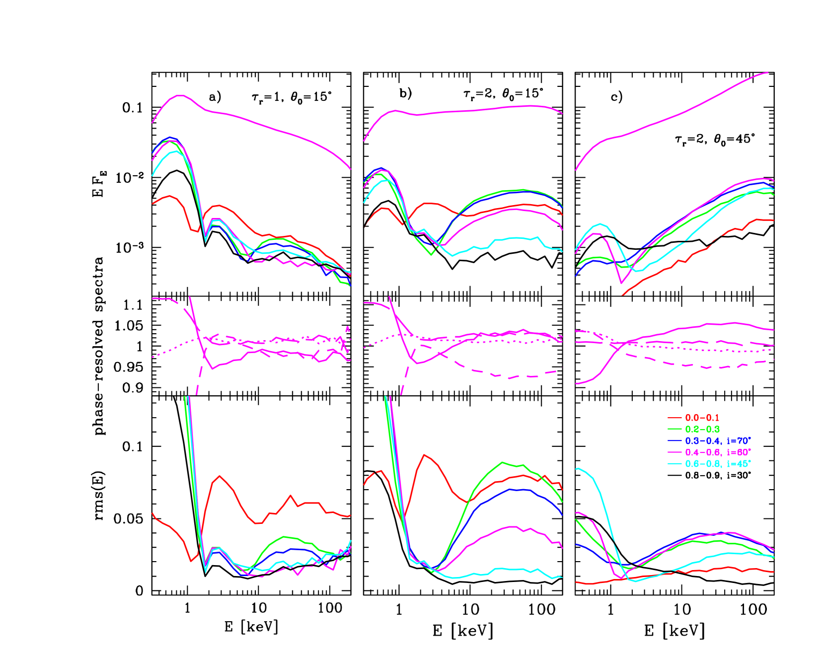
Figure 3: Compton scattered spectra and QPO variability for geometry 1) (precession axis perpendicular to the plane of the outer disc). Columns a), b), c) show the results for different torus parameters: radial optical thickness, $\tau_{\rm r}$, and the half-opening angle $\theta_{0}$, as labelled. The top panels in each column show the time averaged spectrum at the viewing angle $i=60^{\circ}$ (topmost, magenta curve) and the QPO spectra for different viewing angle, as labelled (description in bottom panel, column c). The middle panels show the QPO-phase resolved spectra at four phases separated by $90^{\circ}$, normalized to the time averaged spectrum, at $i=60^{\circ}$, to demonstrate the range of spectral variability. The bottom panels show the fractional ${\rm rms}(E)$ amplitude for different viewing angle. See Sec 3.2.1 for details.

We assume that the hot inner flow forms a torus with a wedge-like cross-section (Fig. 1), with the half-opening angle, $\theta_{0}$, measured from the equatorial plane. The inner boundary, at $r_{1}$, is assumed cylindrical, while the outer boundary, at $r_{2}$, is spherical. The outer cold disc extends from $r_{\rm disc}\approx r_{2}$ outwards. The hot torus precesses around a precession axis, with (constant) precession angle (polar angle between the axis of the torus and the precession axis) $\theta_{p}$. As discussed in Introduction the precession axis itself can be 1) perpendicular to the plane of the outer disc, or 2) it can be inclined to the plane by the same angle $\theta_{p}$. The major difference between the two geometries is that in scenario 1) the relative geometry of the hot torus and the cold disc does not change with the precession phase, while it does change in geometry 2). In fact, in scenario 2), at one particular phase of precession, the equatorial planes of the hot flow and the cold disc may overlap, so the former is not inclined to the latter. There is one more parameter in scenario 2), which is the azimuthal position angle of the precession axis, $\phi_{0}$. We use a convension that $\phi_{0}=0^{\circ}$ means that the precession axis is directed towards the observer (Fig. 1a) while $\phi_{0}=180^{\circ}$ means that the precession axis is directed away from the observer (Fig. 1b). Schematic representation of the geometry can also be seen in Ingram & Done (2012b; fig 1) and in fig 2 in Veledina et al. (2013), where the angle $\beta$ corresponds to our $\theta_{p}$.

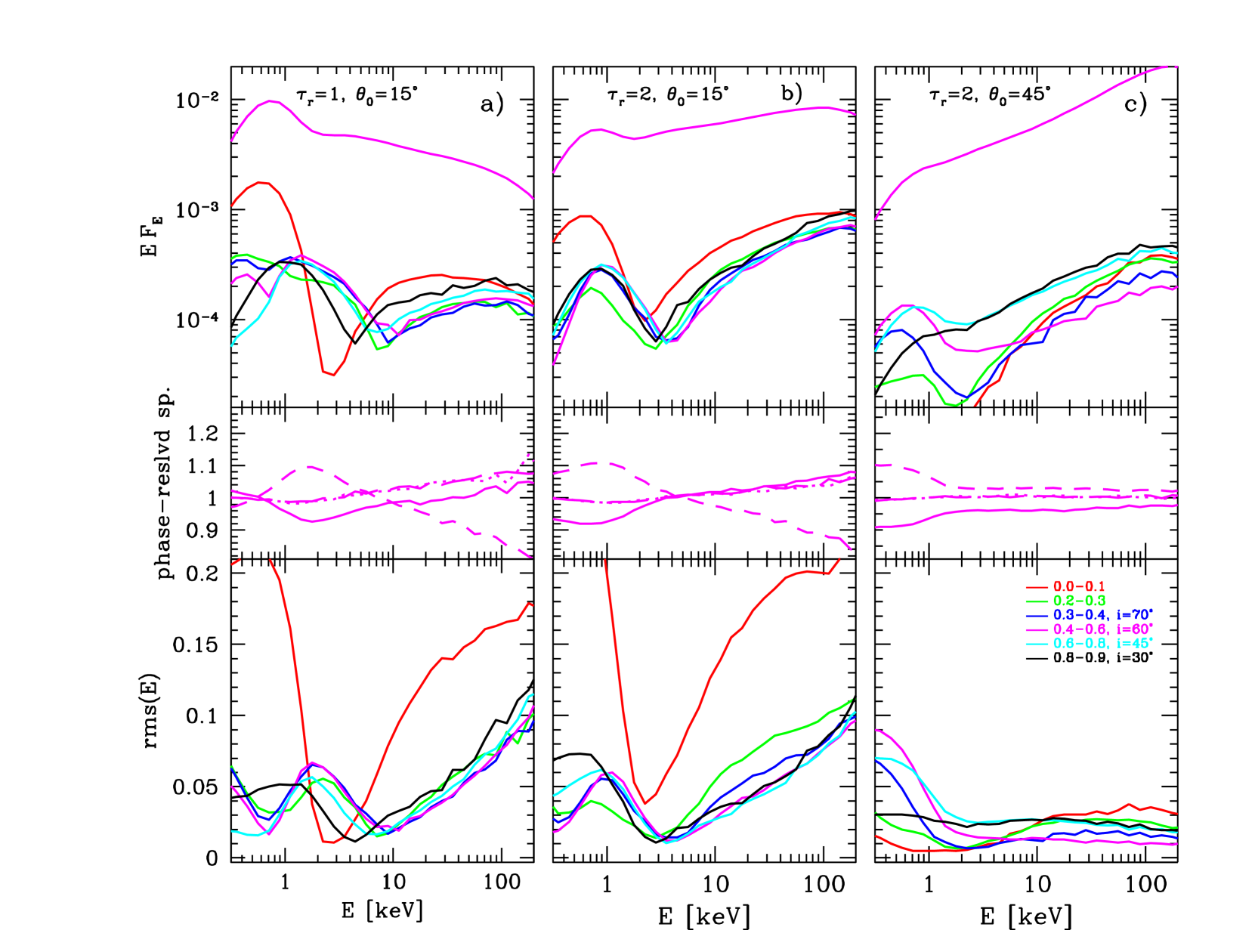
Figure 4: Compton scattered spectra and QPO variability for geometry 2), for the case of $\phi_{0}=0^{\circ}$ (precession axis inclined wrt to the outer disc normal, directed towards the observer; see fig 1a). Columns a), b), c) show the results for different torus parameters: $\tau_{\rm r}$ and $\theta_{0}$, as labelled. The top panels in each column show the time averaged spectrum at the viewing angle $i=60^{\circ}$ (topmost, magenta curve) and the QPO spectra for different viewing angle, as labelled in the bottom panel c). The middle panels show the QPO-phase resolved spectra at four phases separated by $90^{\circ}$, normalized to the time averaged spectrum, at $i=60^{\circ}$. The bottom panels show the ${\rm rms}(E)$ amplitude for different viewing angle.

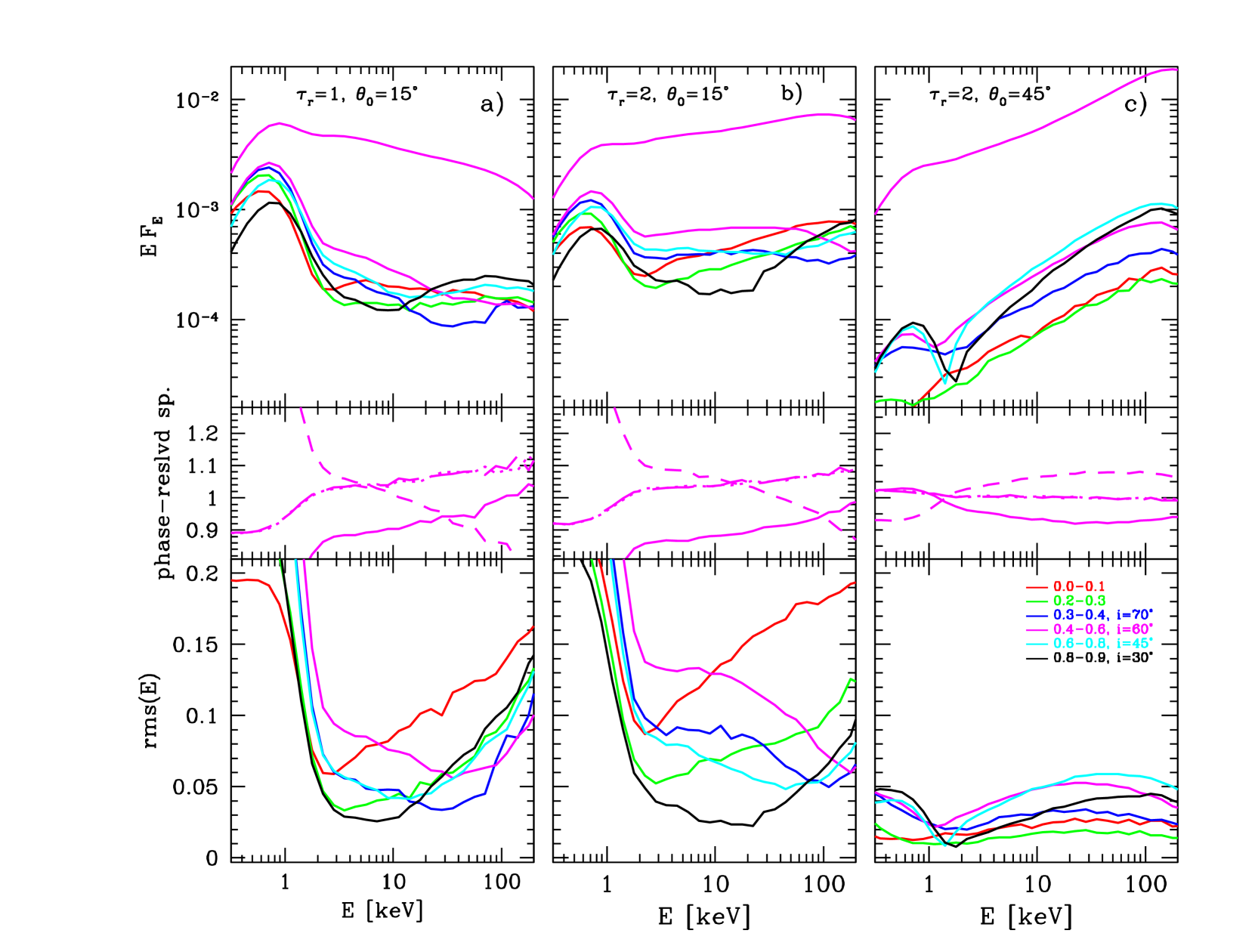
Figure 5: Compton scattered spectra and QPO variability for geometry 2), for the case of $\phi_{0}=180^{\circ}$ (precession axis inclined wrt to the outer disc normal, directed away from the observer; see fig 1b). Columns a), b), c) show the results for different torus parameters: $\tau_{\rm r}$ and $\theta_{0}$, as labelled. The top panels in each column show the time averaged spectrum at the viewing angle $i=60^{\circ}$ (topmost, magenta curve) and the QPO spectra for different viewing angle, as labelled in the bottom panel c). The middle panels show the QPO-phase resolved spectra at four phases separated by $90^{\circ}$, normalized to the time averaged spectrum, at $i=60^{\circ}$. The bottom panels show the ${\rm rms}(E)$ amplitude for different viewing angle.

The optical thickness of the hot plasma in the radial direction is $\tau_{r}$, the thickness in other directions following from the assumed uniform density of the plasma, and corresponding dimensions. The cold disc is assumed to radiate a local blackbody emission, with the standard radial temperature profile $T(r)\propto r^{-3/4}$, i.e. we neglect any boundary effects (e.g., illumination). Consistently, we neglect the hard X-ray component reflected/reprocessed by the cold disc. The local disc emission is assumed isotropic. The maximum disc temperature, at $r=r_{\rm disc}$, is denoted $T_{0}$.

2.2 Monte Carlo comptonization code

The code was already described in Janiuk, Czerny & Życki (2000). It uses the standard prescriptions of Pozdnyakov, Sobol & Syunyaev (1993) and Górecki & Wilczewski (1984) for simulating the inverse Compton scattering of soft photons in a hot plasma. We implemented a range of geometries, allowing the soft photons to originate both inside the hot plasma and outside it (as is the present case). The code assumes uniform plasma density and temperature and it does not include the X-ray reflection from the outer disc. In the present case we consider full 3-D geometry, schematically shown in Fig. 1.

3 Results

The inner hot flow is quite likely to be geometrically thick, so we consider the cases of $\theta_{0}=15^{\circ}$ ($h/r\approx 0.3$) and $\theta_{0}=45^{\circ}$ ($h/r=1$). The absolute (physical) values of the inner and outer torus radii would be important for determination of the plasma temperature (through the heating-cooling balance), but with our simplified treatment of the temperature we use dimentionless units. Nevertheless, the ratio $r_{2}/r_{1}$ is important and we assume $r_{1}=6$ and $r_{2}=30$. The precession angle is assumed $\theta_{p}=15^{\circ}$, while $T_{0}=0.2\,$keV. We compute a sequence of spectra corresponding to different phases of precession and calculate the r.m.s. amplitude of variability as a function of photon energy in the usual way.

3.1 Plasma temperature

The hot torus intercepts a fraction of the soft photons from the cold disc. In the geometrical scenario 1) this fraction is constant as a function of precession phase, while it does vary in geometry 2). This is demonstrated in Fig. 2, where we plot the ratio of luminosity intercepted by the torus to the total luminosity emitted by the disc, for two values of $\theta_{0}$.

The intercepted luminosity is $\approx 10\%$, for all considered parameters. In the scenario 2), and for the geometrically thick torus, $\theta_{0}=45^{\circ}$, the variations are very small, $\approx 2\%$. This is because, for $\theta_{p}<\theta_{0}$ (i.e., the torus is geometrically thicker than the range of its wobble due to precession), only the outer torus boundary is visible from the outer disc, irrespective of the precession phase. Thus, the effective solid angle of the torus from the outer disc is approximately constant, considering that the disc emission is concentrated towards its inner edge. Variations are somewhat larger, $\approx 20\%$, for the thinner torus, when the effective solid angle of the torus does depend on the degree of misalignement of the torus and disc planes.

The varying fraction of the intercepted soft flux implies variations of the plasma temperature, $kT$, since it affects the heating to cooling ratio of the plasma, $l_{\rm h}/l_{\rm s}$. Physical values of $l_{\rm h}$ and $l_{\rm s}$ would depend on the details of energy generation in the flows, most importantly the radial energy generation rates and the transition radius, $r_{2}=r_{\rm disc}$. Detailed considerations of these processes are clearly beyond the scope of this paper, therefore here we simply assume a constant value of $l_{\rm h}$, and $l_{\rm s}$ varying as described above.

We estimate variations of $kT$ adopting Comptonization formulae from Beloborodov (1999a), with $\tau_{T}=1$ and $\delta=1/6$. The average $l_{\rm h}/l_{\rm s}$ ratio is assumed such that the resulting plasma temperature is close to 100 keV, as observed in the accreting sources. The temperature is constant in geometry 1) as the seed photons are constant with phase, but the change in $l_{\rm s}$ for geometry 2) means that $kT(\phi)$ also changes by around 10%, as shown in Fig. 2 (dotted line).

3.2 Variability amplitude

Here we present the fractional amplitude of variability (containing both the main QPO and its all harmonics) as a function of energy, in the two considered scenarios for the precession geometry. We want to compare our simulations with the observations which show subtle changes in QPO shape relative to the Compton scattered continuum (Axelsson et al. 2014; Axelsson & Done 2016). Hence we plot only the Compton scattered spectra and its variability, and do not include the constant disc component which will dilute the fractional variability of both the QPO and broadband variability at low energies.

We consider two values of the radial optical thickness of the torus, $\tau_{r}=1,2$ and two values of the torus shape, parameterized by $\theta_{0}$, with $\theta_{0}=15^{\circ}$ and $45^{\circ}$. We combine these torus parameters into three cases, $\tau_{r}=1$, $\theta_{0}=15^{\circ}$; $\tau_{r}=2$, $\theta_{0}=15^{\circ}$ and $\tau_{r}=2$, $\theta_{0}=45^{\circ}$, resulting in a broad range of the “effective” optical thickness of the torus, which determins the slope of the final Comptonized spectrum.

3.2.1 Geometry I. Precession axis perpendicular to the outer disk

The results are plotted in Fig. 3. Three columns of the plot show the three cases of the “effective” optical thickness. The top panels of each column present the time average spectrum at the viewing angle $i=60^{\circ}$ (the top magenta curve) and the QPO spectra (i.e., the variable components), for different viewing angle as labelled (viewing angle labels in the bottom panel, column c).

The middle panels show the QPO-phase resolved spectra, at four values of the QPO phase separated by $90^{\circ}$, normalized to the time averaged spectrum, at $i=60^{\circ}$, to demonstrate the range of spectral variability.

The bottom panels show the ${\rm rms}(E)$ amplitude for different viewing angle.

The highest amplitude of the Comptonized component alone is actually observed at energies corresponding to seed photon spectrum. Related to this, there is a pronounced bump in rms$(E)$, especially for high viewing angle for thin torus ($\theta_{\rm p}=15^{\circ}$), at energies corresponding to the first scattering in the Comptonized spectrum. As the torus orientation changes relative to the observer, the effective optical thickness along the line of sight changes. This results in a variable fraction of scattered and unscattered photons. The change of effective $\tau$ (“effective” meaning integrated over all lines of sight leading to different points on the emitting disc) depends on the viewing angle. For high viewing angle (close to “edge on”) the change is large, since depending on the torus position, an observer may see through the entire torus, or very little of it. For lower viewing angle (close to “top view”) there is still a large amplitude of variability of the un-scattered component, because of the possibility of (part of) the torus to be in the line of sight at a particular precession phase. However, the observed scattered component will have reached observer after changing its direction of motion by about $90^{\circ}$. Photons originating at any azimuthal angle are approximately equally likely to achieve this, so such a component will only be weakly variable with the precession phase. Obviously, the observed amplitude at energies of the seed photons is strongly suppressed when the directly observed, constant disc emission is added (Fig. 3).

The feature in rms$(E)$ due to first scattering is very prominent for low $\tau$ and/or high viewing angle situations. However, its strength might be a consequence of the simplifying assumptions of the model, most importantly the uniform temperature and density of the plasma. The situation might be reminiscent of that from early studies of Comptonized spectra (e.g., Stern et al. 1995). These predicted strong first-scattering feature in the spectrum, which was not observed in X-ray data. It was later realized that a realistic geometry would be rather non-uniform and that would most likely smear out such features.

Where the first-scattering feature is not so prominent, the rms$(E)$ increases somewhat with energy (at least for viewing angles $\geq 30^{\circ}$), up to a maximum at 20–40 keV, then it decreases again. This behaviour reflects the subtle changes of the spectrum, as the changing orientation of the torus means it is observed at changing viewing angle. The variability is stronger for larger $\tau_{r}$ (right vs. left panels in Fig. 3), at least when the line of sight passes through the torus, because the transmitted fraction, $e^{-\tau}$, is more variable. At low viewing angles the variability is generally weaker, since the emission is closer to isotropy. The energy dependence is also weaker, the rms spectra being either independent of energy or slighly deceasing with $E$.

Variability is weaker for geometrically thicker torus (right vs. left panels in Fig. 3). At high viewing angle the reason for this is that now the optical depth along the line of sight does not change much, as the range of torus “wobble” (due to precession) is small compared to torus angular size. At low viewing angle, the reason is rather different, namely it is the higher degree of isotropy of emission for thicker (geometrically hence also optically) torus.

3.2.2 Geometry II. Precession axis tilted to the outer disk

In this scenario there is one additional parameter, which is the location of the observer relative to the precession axis. The location can be parameterized by the position angle of the precession axis, $\phi_{0}$, i.e. the angle between the plane of the precession axis and outer disc normal, and the plane of the line of sight and the outer disc normal (angle $\phi$ in fig 2 of Veledina et al. 2013; see Fig 1). For $\phi_{0}$ close to $0^{\circ}$ the observer (especially positioned close to top-view) may see only the top of the torus and never see its outer boundary, while for $\phi_{0}$ close to $180^{\circ}$ the observer may see the outer boundary for a significant fraction of precession period. Obviously, situations with $\phi_{0}$ and $360^{\circ}-\phi_{0}$ are equivalent. Figures 4–5 show the resulting rms$(E)$ dependencies for different $\phi_{0}$.

In this geometry the amplitude of variability can be expected to be larger than in geometry I. There are two obvious reasons for this, both related to the variable number of soft photons entering the hot precessing torus. The mere fact that the numer of soft photons varies causes additional variability of the normalization of the overall Comptonized spectrum. Then there is the additional spectral variability caused by temperature variations of the plasma. However, the obvious correlation between these two parameters (Fig. 2), and the complicated dependence of the spectrum on the precession angle (Sec. 3.2.1) mean that the resulting rms$(E)$ is rather complicated. In particular, the influence of the temperature variations is rather different for $\phi_{0}=0^{\circ}$ and for $\phi_{0}=180^{\circ}$. The total variability amplitude is 4-10% for our parameters which approximately matches the observed range of values.

The results show a complicated dependence of rms$(E)$ on the viewing angle. The dependence is actually rather weak when mostly top/bottom torus walls are observed, as is the case of $\phi_{0}=0$ at not-too-high viewing angle (Fig 4a,b), or when the torus emits almost isotropically because of larger optical depth (Fig 4c; Fig 5c). However, there is a significant dependence on $i$ when during the torus precession an observer sees both the outer and upper torus walls (Fig 5a,b).

4 Discussion

The Lense-Thirring precession appears to be an attractive model for the low-frequency QPO observed in black hole binaries. Current magnetohydrodynamical simulations reveal that a hot torus-shaped plasma can precess as a solid body (Fragile et al. 2007), with frequencies matching those observed in black hole X-ray binaries (Ingram et al. 2009). This precessing hot torus scenario fits well into the overall geometry envisioned for the hard state of X-ray binaries, where a trucated disk and a hot inner flow seems to be the most complete scenario, explaining, at least at the phenomenological level, a range of observational data both in the spectral and time domain (review, e.g., in Done et al. 2007). The recent detection of the predicted iron line energy modulation with QPO phase (Ingram et al. 2016a) gives strong support to this model.

The most important variability characteristic presented in this paper is the energy dependence of the amplitude of variability. The model fractional rms$(E)$ does not generally show a clear monotonic dependence. There are various effects influencing the rms$(E)$, like the seed photon contribution and the first scattering effects. Also, if the precession results in the observer seeing both the top and the outer torus boundary, the rms$(E)$ seems to be more complicated than in the simpler case (cf Fig. 4 and Fig. 5 and panels a) and b) in Fig. 1), although in a realistic situation the hot plasma may form a rather smoother structure, which may influence the details of rms$(E)$. There are nevertheless regions of parameter space where rms$(E)$ does increase, which can also be represented as the QPO energy spectrum being harder than the time averaged spectrum. The character of the simulated rms$(E)$ relation can be expected to be only weakly dependent on the spectral shape, as the mechanism of the modulation is independent of the spectral formation.

Observationally, an interesting anticorrelation seems to exist between the spectral shape (slope) of the time averaged and the QPO spectrum: the QPO spectrum is harder than the time averaged spectrum in the soft spectral state of a source, while the QPO spectrum is softer than the time averaged spectrum when the source is in a hard specral state (e.g., Sobolewska & Życki 2006; Axelsson et al. 2014; Axelsson & Done 2016). Simple analysis performed by Życki & Sobolewska (2005) suggests that the two types of behaviour correspond to two different driving parameters of the oscillations, for example, either by the plasma heating rate or the cooling rate. A particular geometrical scenario considered in Życki & Sobolewska (2005), namely a modulation of the covering factor of the cold reflecting plasma (e.g. the cold disc), predicted the QPO spectrum being softer than the time averaged spectrum.

The Lense-Thirring precession model is a different geometrical model, though, and for some parameters it does predict the QPO spectrum harder than the time averaged specrum, as mentioned above. This happens for a range of torus shapes, producing both hard and soft time averaged spectra. It is therefore uncertain that it would be possible to construct such a series of models that would on one hand predict spectral hard–soft state evolution and, consistently the QPO spectrum evolution.

The model predicts also a significant variability of the seed photons component. This is because of the varying observed fraction of the disc component transmitted through the precessing torus. The observed soft emission would obviously be a sum of the transmitted fraction and the directly observed disc emission and the latter dominates over the former (the intercepted fraction is about 10%, Fig. 1) and so the observed variability amplitude would be negligible at the seed photon energy, as indeed observed.

Figure 6: Relation between the spectral slope of the Comptonized emission, $\Gamma$, and the QPO frequency, as a function of the transition radius between the outer disc and the precessing torus, $r_{2}$, for black hole spin $a=0.9$. The spectral slope depends on $r_{2}$ through the plasma heating-to-cooling ratio, while $f_{\rm QPO}$ depends on $r_{2}$ because the precessing torus moment of inertia depends on $r_{2}$ (Ingram et al. 2009). See Discussion for details.

The presented Lense-Thirring precession model can also qualitatively reproduce the correlation between the spectral slope and the QPO-frequency. Adopting a simple description of the energy generation in the accretion flow,

$$F_{\rm grav}(r)\propto\left(1-\sqrt{r_{1}\over r}\right){1\over r^{3}},$$ (1)

where the inner radius of the precessing torus is given as $r_{1}=3.0(h/r)^{-4/5}a^{2/5}$ (Ingram et al. 2009 and references therein), we can describe the heating-cooling balance of the hot plasma as a function of the transition radius, $r_{2}$:

$$l_{\rm h}(r_{2})\propto\int_{r_{1}}^{r_{2}}rF_{\rm grav}(r)dr,$$ (2)

and $l_{\rm s}(r_{2})=0.1[l_{\rm tot}-l_{\rm h}(r_{2})]$, where $l_{\rm tot}=\int_{{\rm r}_{1}}^{\infty}rF_{\rm grav}(r)\,dr$, and the numerical factor 0.1 accounts for the fraction of soft photons intercepted by the hot flow (Fig. 2). Using $\Gamma=2.33(l_{\rm h}/l_{\rm s})^{-1/6}$ (Beloborodov 1999b) and combining it with Eq. 2 in Ingram et al. (2009) we can obtain a simple example of the $\Gamma$-$f_{\rm QPO}$ relation, for a given value of $a$ (Fig. 6). Obviously, Eq. 1 is a rather ad hoc generalization of the simple formula for gravitational energy dissipation in Keplerian disc in Schwarzschild metric, so it should not be relied upon to provide a robust quantitative relation. However, it does capture the trend and the right range of both parameters.

The presented computations are admittedly simplified in some aspects. Most importantly the Comptonizing plasma is uniform in density and temperature, and the situation described is quasi-static. In more realistic scenarios the overall variability would come from perturbations of mass accretion rate propagating radially through the flow. A perturbation in mass flow may result in a perturbation of plasma temperature propagating inwards, leading to spectral evolution superposed on the geometrical effect. This may remove from the spectra the signatures of the first scattering, which are generally not observed (e.g., Stern et al. 1995). These more complicated scenarios should be considered in detail to see whether they may account for the whole range of observed behaviour.

References

- [] Axelsson M., Done, C., 2016, MNRAS, 458, 1778
- [] Axelsson M., Done, C., Hjalmarsdotter L., 2014, MNRAS, 438, 657
- [] Bardeen J. M., Petterson J. A., 1975, ApJ, 195, L65
- [] Beloborodov A. M., 1999a in High Energy Processes in Accreting Black Holes, ASP Conference Series 161, ed. J. Poutanen & R. Svensson, p.295 (arXiv:astro-ph/9901108)
- [] Beloborodov A. M., 1999b, ApJ, 510, L123
- [] Churazov E., Gilfanov M., Revnivtsev M., 2001, MNRAS, 321, 759
- [] Done C., Gierliński M., Kubota A., 2007, A&AR, 15, 1
- [] Fragile P. C., Mathews G. J., Wilson J. R., 2001, ApJ, 553, 955
- [] Fragile P. C., Blaes B. M., Anninos P., Salmonson J. D., 2007, ApJ, 668, 417
- [] Górecki A., Wilczewski W., 1984, AcA, 34, 141
- [] Ingram A., Done C., 2011, MNRAS, 415, 2323
- [] Ingram A., Done C., 2012a, MNRAS, 419, 2369
- [] Ingram A., Done C., 2012b, MNRAS, 427, 934
- [] Ingram A., Done C., Fragile P. C., 2009, MNRAS, 397, L101
- [] Ingram A., Maccarone T. J., Poutanen J., Krawczynski H., 2015, ApJ, 807, 53
- [] Ingram A., van der Klis M., Middleton M., Done c., Altamirano D., Heil L., Uttley P., Axelsson M., 2016a, MNRAS, 461, 1967
- [] Ingram A., van der Klis M., Middleton M., Altamirano D., Uttley P., 2016b, MNRAS, in press (arXiv:1610.00948 [astro-ph.HE])
- [] Janiuk A., Czerny B., Życki P. T., 2000, MNRAS, 318, 180
- [] Pottschmidt K. et al., 2003, A&A, 407, 1039
- [] Pozdnyakov L. A., Sobol I. M., Syunyaev R. A., 1983, ASPRv, 2, 189
- [] Remillard R. A., McClintock J. E., 2006, A&AS, 38, 903
- [] Sobolewska M., Życki P. T., 2006, MNRAS, 370, 405
- [] Stella L., Vietri M., 1998, ApJ, 492, L59
- [] Stern B. E., Poutanen J., Svensson R., Sikora M., Begelman M. C., 1995, ApJ, 449, L13
- [] Veledina A., Poutanen J, 2015, MNRAS, 448, 939
- [] Veledina A., Poutanen J, Ingram A., 2013, ApJ, 778, 165
- [] Życki P. T., Sobolewska M., 2005, MNRAS, 364, 891