Exact solution of the critical Ising model with special toroidal boundary conditions.

Abstract

The Ising model in two dimensions with special toroidal boundary conditions is analyzed. These boundary conditions, which we call duality twisted boundary conditions, may be interpreted as inserting a specific defect line (“seam”) in the system, along non-contractible circles of the cylinder, before closing it into a torus. We derive exact expressions for the eigenvalues of a transfer matrix for the critical ferromagnetic Ising model on the M x N square lattice wrapped on the torus with a specific defect line. As a result we have obtained analytically the partition function for the Ising model with such boundary conditions. In the case of infinitely long cylinders of circumference L with duality twisted boundary conditions we obtain the asymptotic expansion of the free energy and the inverse correlation lengths. We find that the ratio of subdominant finite-size correction terms in the asymptotic expansion of the free energy and the inverse correlation lengths should be universal. We verify such universal behavior in the framework of a perturbating conformal approach by calculating the universal structure constant $C_{n1n}$ for descendent states generated by the operator product expansion (OPE) of the primary fields. For such states the calculations of an universal structure constants is a difficult task, since it involves knowledge of the four-point correlation function, which in general is not fixed by conformal invariance except for some particular cases, including the Ising model.

1 Introduction

Finite-size corrections and scaling for critical lattice systems, initiated more than four decades ago by Ferdinand, Fisher, and Barber ferdinand ; FerdFisher ; barber have attracted much attention in intervening decades (see Refs. privman ; hu for reviews). Finite-size effects are of practical interest due to recent progress in fine processing technologies, which has enabled the fabrication of nanoscale materials with novel shapes nano1 ; nano2 ; nano3 . As soon as one has a finite system one must consider the question of boundary conditions on the outer surfaces or “walls” of the system. As is well known, the critical behavior near boundaries normally differs from the bulk behavior.

To understand the effects of boundary conditions, it is especially valuable to study model systems which have exact results (for more details, see Igloi ). Two-dimensional models of statistical mechanics have long served as a proving ground in attempts to understand critical behavior and to test the general ideas of finite-size scaling. Very few of them have been solved exactly and the Ising model is the most prominent example. Since Onsager obtained the exact solution of the two-dimensional Ising model with cylindrical boundary conditions in 1944 Onsager , exact treatments of Ising models on different two-dimensional surfaces have been continuously attempted to address different two-dimensional topologies Kaufman ; LuWu2001 ; LuWu1998 ; Liaw ; Brascamp ; Brien . The partition function for the Ising model on finite lattices has been calculated exactly for many different boundary conditions, including toroidal Kaufman , the Mobius strip and the Klein bottle LuWu2001 , as well as self-dual LuWu1998 , helical Liaw , and Brascamp and Kunz boundary conditions Brascamp . Additionally systems with cylindrical boundary condition in one direction and free, fixed and mixed boundary condition in another direction have been investigated Brien .

The Ising model with a defect line goes back at least to Bariev Bariev and McCoy and Perk Mccoy . The interpretation in terms of conformal invariance was started by Turban Turban and Henkel and Patkos Henkel1 . Recently, there has been much progress on understanding conformal boundary conditions in rational conformal field theories. This has been caused by its relevance in string and brane theory on the one hand, and in various problems of statistical mechanics and condensed matter on the other. For $sl(2)$ minimal theories, a complete classification has been given Behrend ; Behrend1 of the conformal boundary conditions on a cylinder. A complete classification of the conformal boundary condition on the torus has also been given Affleck1997 ; Affleck1996 ; Petkova ; Chui . The key idea is to compute the partition function on a torus by identifying the states at the two ends of a cylinder through the trace operation. This may be interpreted as inserting defect line into the system along non contractible circles of the cylinder, before closing it into a torus. The effect of this operation is to “twist” the boundary conditions. In statistical mechanics, this is a familiar operation, often referred to as a “seam”.

In this paper we reported the exact solution of the critical Ising model in two dimensions with a specific defect line. We note that some preliminary results of our investigations have already been announced in a letter pki . Our goal is not to discuss defect lines in general, but rather to specialize to a very peculiar type, namely the only one which can be treated in terms of unitary representations of the $c=1/2$ Virasoro algebra. Note that in general there are an infinite set of boundary conditions associated with defects Affleck1996 ; Affleck1997 , which can all be described in terms of unitary representations of the $c=1$ Virasoro algebra. The principle of unitarity of the underlying field theory restricts, through the Kac formula, the possible values of the central charge $c$, and the highest conformal dimensions $\Delta$ and $\bar{\Delta}$. For the 2D Ising model, we have $c=1/2$ and the only possible values are $\Delta,\bar{\Delta}=0,1/16,1/2$.

A central element of the modern theory of bulk critical phenomena is the division into (bulk) universality classes. In general, each bulk universality class of critical phenomena splits into several boundary universality classes. For the Ising universality class there are nine different boundary universality classes. Three of them are associated with the strip geometry and nine boundary universality classes are associated with the cylinder geometry.

The study of boundary conditions in conformal field theories has attracted much attention in recent decades. The original papers by Cardy and Lewellen Cardy1991 and Cardy Cardy1989 on boundary conformal field theory set out the basic properties. For the Ising universality class, which corresponds to a conformal field theory with central charge $c=1/2$, there are three highest weight representations with weights $(0,1/2,1/16)$, corresponding to the bulk primary operators ($\mathbb{I},\epsilon,\sigma$) representing the unit operator, the energy density and the magnetization, respectively. Thus for the Ising model on a plane we have three different conformally invariant boundary conditions: when the boundary spins are all fixed up, all fixed down or all are free. They can be denoted by $(+),(-)$ and $(f)$ and they correspond to the conformal dimensions $0,1/2,1/16$, respectively. In the strip geometry we have three different pairs of boundary conditions related by fusion rules to the three possible values of the conformal dimensions $0,1/16,1/2$ Cardy1989 . For example $(--),(-+)$ and $(-f)$ are related to the conformal dimensions $0,1/2$ and $1/16$, respectively in agreement with Ising fusion rules

$$\epsilon\otimes\epsilon = \mathbb{I}$$

$$\epsilon\otimes\sigma = \sigma$$

$$\epsilon\otimes\mathbb{I} = \epsilon.$$ (1)

Thus for the Ising model in the strip geometry we have three different conformally invariant boundary conditions with the conformal dimension $\Delta$ equal to

$$\Delta = 0\hskip 36.98866pt\mbox{for free, fixed $(++)$ or $(--)$ boundary conditions}$$ (2)

$$\Delta = \frac{1}{2}\hskip 34.14322pt\mbox{for fixed $(+-)$ or $(-+)$ boundary conditions}$$ (3)

$$\Delta = \frac{1}{16}\hskip 28.45274pt\mbox{for mixed boundary conditions.}$$ (4)

For fixed $(++)$ (or $(+-)$) boundary conditions the spins are fixed to the same (or opposite) values on two sides of the strip. Mixed boundary conditions correspond to free boundary conditions on one side of the strip, and fixed boundary conditions on the other. In the terminology of surface critical phenomena (for a general review of critical behavior at surfaces, see Binder ) these three boundary universality classes: free, fixed $(+-)$ and mixed correspond to “ordinary”, “extraordinary” and “special” surface critical behavior, respectively.

Let us now consider the Ising model on a torus defined by modular parameter $\tau=\tau_{1}+i\tau_{2}$. The partition function of the Ising model in CFT can be written as

$$Z_{\rm Ising}={\rm Tr}\,e^{-2\pi\tau_{2}\left(L_{0}+\bar{L}_{0}-\frac{1}{24}\right)+2\pi i\tau_{1}\left(L_{0}-\bar{L}_{0}\right)}$$ (5)

where $L_{0},\bar{L}_{0}$ are the Virasoro generators. In terms of the eigenvalues of $L_{0}$ and $\bar{L}_{0}$ we can rewrite the partition function in the form

$$Z_{\rm Ising}=\sum_{\alpha}e^{-2\pi\tau_{2}\left(\Delta_{\alpha}+\bar{\Delta}_{\alpha}-\frac{1}{24}\right)+2\pi i\tau_{1}\left(\Delta_{\alpha}-\bar{\Delta}_{\alpha}\right)}=\sum_{\alpha}e^{-2\pi\tau_{2}\left(h_{\alpha}-\frac{1}{24}\right)+2\pi i\tau_{1}s_{\alpha}},$$ (6)

where $\Delta_{\alpha},\bar{\Delta}_{\alpha}$ are the holomorphic and antiholomorphic conformal dimensions of the scaling operators $\phi_{\alpha}$ and $h_{\alpha}=\Delta_{\alpha}+\bar{\Delta}_{\alpha}$ and $s_{\alpha}=\Delta_{\alpha}-\bar{\Delta}_{\alpha}$ are known as scaling dimension and conformal spin of $\phi_{\alpha}$ respectively. The scaling operators come in conformal towers built up from the primary operators. If $\Delta,\bar{\Delta}$ are the conformal dimensions of a primary operator, then the scaling operators in its conformal tower have conformal dimensions of the form $\Delta_{n}=\Delta+n$ and $\bar{\Delta}_{m}=\bar{\Delta}+m$, where $n,m\in\mathbb{N}$. The universal part in finite size corrections of the ground state energy expected from conformal field theory depends on the central charge $c$, the scaling dimension $h=\Delta+\bar{\Delta}$ and conformal spin $s=\Delta-\bar{\Delta}$ of the ground state. The scaling dimension $(h)$ and the conformal spin $(s)$ of the ground stateare are the universal constants, but may depend on the boundary conditions. In the case of the Ising model ($c=\frac{1}{2}$) the conformal dimensions $\Delta,\bar{\Delta}$ can take the values $0,\frac{1}{2}$ and $\frac{1}{16}$. Thus for the Ising model on an infinitely long cylinder there are nine possible values of the pair of the conformal dimensions $(\Delta,\bar{\Delta})$ and as a consequence nine different boundary conditions. Three of them with conformal spin $s=0$ and the remaining six can be combined into three pairs which can be identified by the absolute value of the conformal spin. Thus for the Ising model on the infinitely long cylinder we have following nine boundary conditions:

$$(\Delta,\bar{\Delta}) = (0,0)\hskip 51.21504pt\mbox{for periodic boundary conditions}$$ (7)

$$(\Delta,\bar{\Delta}) = \left(\frac{1}{16},\frac{1}{16}\right)\hskip 28.45274pt\mbox{for antiperiodic boundary conditions}$$ (8)

$$(\Delta,\bar{\Delta}) = \left(\frac{1}{2},\frac{1}{2}\right)\qquad$$ (9)

$$(\Delta,\bar{\Delta}) = \left(\frac{1}{16},0\right)\,\mbox{and}\,\left(0,\frac{1}{16}\right)\hskip 14.22636pt\mbox{for duality-twisted boundary conditions}$$ (10)

$$(\Delta,\bar{\Delta}) = \left(\frac{1}{2},0\right)\,\mbox{and}\,\left(0,\frac{1}{2}\right)\qquad$$ (11)

$$(\Delta,\bar{\Delta}) = \left(\frac{1}{2},\frac{1}{16}\right)\,\mbox{and}\,\left(\frac{1}{16},\frac{1}{2}\right)\qquad$$ (12)

Note that the pairs of boundary conditions listed in Eqs. (10) - (12) [e.g. $\left(\frac{1}{16},0\right)$ and $\left(0,\frac{1}{16}\right)$] can be referred to as complex conjugate boundary conditions following terminology of the Refs. Grimm ; Grimm1993 .

Past efforts have been focused mainly on periodic and antiperiodic boundary conditions. Little attention has been paid to the boundary condition given by Eqs. (9) - (12). In this paper we will try to fill partially this gap and consider one of these sets of boundary conditions, namely those given by Eq. (10) with $(\Delta,\bar{\Delta})=\left(\frac{1}{16},0\right)$. We will refer to such boundary conditions as duality-twisted boundary conditions since that name have been given to boundary condition with $(\Delta,\bar{\Delta})=\left(\frac{1}{16},0\right)$ for the case of the Ising quantum chain and have been considered in Ref. Schutz . Furthermore, the complete spectrum of the Hamiltonian for finite chains of length $N$ with this set of boundary conditions is obtained exactly Grimm .

Although many theoretical results are now known about the critical exponents and universal relations among the leading critical amplitudes, not much information is available on ratios among the amplitudes in finite-size correction terms Aharony ; Aharony1 ; Aharony2 . New universal amplitude ratios for finite-size corrections of the two-dimensional Ising model on square, triangular and honeycomb lattices with periodic, antiperiodic, free, fixed and mixed boundary conditions have been recently presented Izmailian2001 ; Izmailian2009a ; Izmailian2009b ; Izmailian2012 ; Izmailian2010 .

In this paper we present a new set of universal amplitude ratios for the finite-size corrections of the two-dimensional Ising model on square lattices for duality twisted boundary conditions and show that such universal behavior is correctly reproduced by the conformal perturbative approach. We also extend the calculation of the universal structure constants for descendent states generated by the OPE of the primary fields. For such states the calculations of the universal structure constants is a difficult task, since it involves the knowledge of the four-point correlation function, which in general does is fix by conformal invariance except for some particular cases, including the Ising model.

Our objective in this paper is to study the Ising model in two dimensions with particular toroidal boundary conditions, the so-called duality-twisted boundary conditions. The paper is organized as follows. In Sec. 2 we introduce the Ising model on the square lattice with duality-twisted boundary conditions. In Sec. 3 we define the transfer matrix of the model. In Sec. 4 we derive exact expressions for the eigenvalues of the transfer matrix for the critical ferromagnetic Ising model on the $M\times N$ square lattice. We also derive the exact expression for the conformal partition function in Sec. 5. In Sec. 6 we consider the limit $N\to\infty$ for which we obtain the expansion of the free energy and inverse correlation lengths for the Ising model on an infinitely long cylinder of circumference $L_{x}$ with duality twisted boundary conditions. We find that ratio of subdominant finite-size correction terms should be universal and in Sec. 7 and Sec. 8 we show that such universal behavior is correctly reproduced by the conformal perturbative approach. Our main results are summarized and discussed in Sec. 9.

2 Ising model with specific defect line (“seam”)

The Ising model is one of the classical models in statistical mechanics. The anisotropic two-dimensional Ising model on a lattice with periodic boundary conditions and with a specific defect line (“seam”) was formulated in Refs. Brien ; Pearce2001 . For the Ising model the seams are labelled by the Kac labels $(r,s)$. There are six possible partition functions $Z_{(r,s)}(q)$ labelled by $(r,s)=(1,1),(1,2),(1,3),(2,1),(2,2),(2,3)$ and for three of them, namely, for the seams $(r,s)=(1,1),(1,2)$ and $(1,3)$, the partition functions $Z_{(r,s)}(q)$ are obtained numerically to very high precision in Pearce2001 :

$$Z_{P}=Z_{(1,1)}(q) = \left|\chi_{0}(q)\right|^{2}+\left|\chi_{\frac{1}{2}}(q)\right|^{2}+\left|\chi_{\frac{1}{16}}(q)\right|^{2}$$ (13)

$$Z_{(1,2)}(q) = \left[\chi_{0}(q)+\chi_{\frac{1}{2}}(q)\right]\chi_{\frac{1}{16}}(q)^{*}+\left[\chi_{0}(q)+\chi_{\frac{1}{2}}(q)\right]^{*}\chi_{\frac{1}{16}}(q)$$ (14)

$$Z_{A}=Z_{(1,3)}(q) = \chi_{0}(q)\chi_{\frac{1}{2}}(q)^{*}+\chi_{0}(q)^{*}\chi_{\frac{1}{2}}(q)+\left|\chi_{\frac{1}{16}}(q)\right|^{2}$$ (15)

where $\chi_{0}\equiv\chi_{0}(q)$, $\chi_{\frac{1}{2}}\equiv\chi_{\frac{1}{2}}(q)$ and $\chi_{\frac{1}{16}}\equiv\chi_{\frac{1}{16}}(q)$ are the chiral characters and $q$ is the modular parameter. The $(r,s)=(1,1)$ and $(1,3)$ seams reproduce the well known partition function of the Ising model with periodic and antiperiodic boundary conditions respectively. In contrast, little attention has been paid to the boundary conditions given by the seam $(r,s)=(1,2)$. In what follows we will give the exact solution for the Ising model with seams $(r,s)=(1,2)$ and show that they correspond to duality-twisted boundary conditions. In our calculations we will follow the method of the Ref. Pearce2001 .

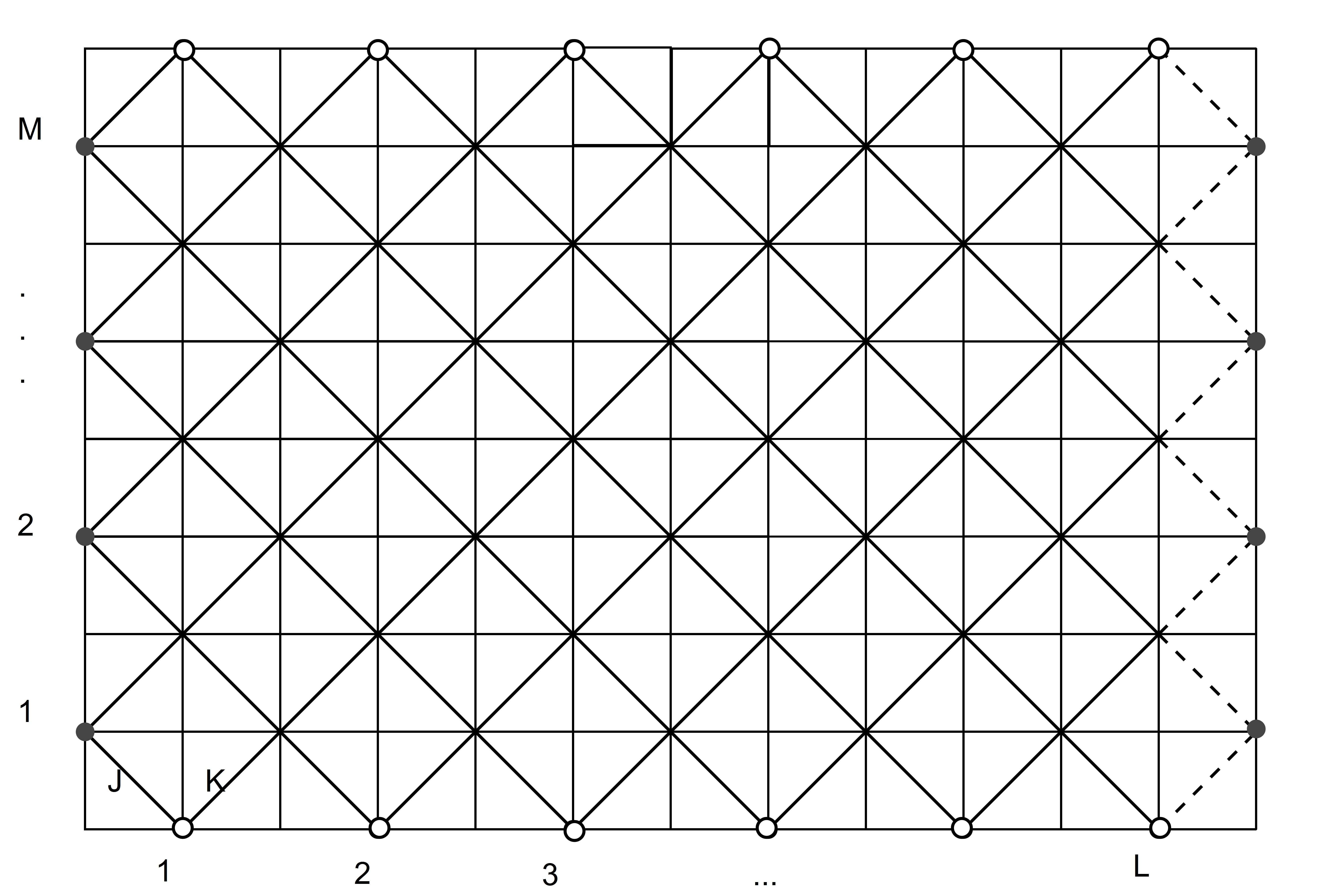
Figure 1: The lattice is constructed with $2L$ regular faces in each row and $2M$ regular faces in each column. The lattice has two sublattices which can be even or odd. The heights are even on the even sublattice and odd on the odd sublattice. On the even sublattice the heights are fixed to the value $2$. On the odd sublattice we identify the state $a=1$ with the usual $+$ Ising state and $a=3$ with the usual $-$ Ising state. The odd sublattice can be considered as the square lattice rotated by $45$ degrees, in which each row has $L$ faces and each column has $M$ faces. The faces on the odd sublattice are twice as large as regular faces. The line defect is inserted along the rightmost columnar edge (dashed line) before closing the lattice into a torus with periodic boundary conditions. Periodic boundary conditions are imposed in both directions.

Let us consider a square lattice rotated by $45$ degrees (Fig. 1), in which each row has $L$ faces and each column has $M$ faces. We insert one defect line (seam) along the last column. The lattice thus consists of $2L-1$ regular (zigzagging) columnar edges and one defect line and $2M$ regular (zigzagging) row edges. Periodic boundary conditions are imposed in both directions and in Fig. 1 this is represented as identifying the light (dark) nodes on the first row (column) with the respective light (dark) nodes on the last row (column). The physical dimensions of the lattice, $L_{x}$ and $L_{y}$, are given by

$$L_{x} = \sqrt{2}\left(L-\frac{1}{2}\right)$$ (16)

$$L_{y} = \sqrt{2}\;M.$$ (17)

The finite-size partition function for the Ising model $Z_{L_{x}L_{y}}$ can be written as

$$Z_{L_{x}L_{y}}=\sum_{s}\exp{\left(J\sum_{\langle ij\rangle}s_{i}s_{j}+K\sum_{\langle ij\rangle}s_{i}s_{j}\right)}$$

where the first sum within the parenthesis is over NW-SE edges, and the second sum over NE-SW edges and spin variable $s_{i}$ can take the two values $\pm 1$. Since we restrict ourselves to the critical Ising model, we have $\sinh(2J)\sinh(2K)=1$. This condition can be conveniently parameterized by introducing a so-called spectral parameter $u$, so that $\sinh(2J)=\cot(2u),\sinh(2K)=\tan(2u)$, with $0<u<\pi/4$. The anisotropy parameter is $\zeta$ related to the spectral parameter $u$ through

$$\xi=\sin 4u.$$ (18)

For the isotropic system $(K=J)$ we have $u=\pi/8$ and $\zeta=1$. Now the finite-size partition function $Z_{L_{x}L_{y}}$ can be rewritten in the following form

$$Z_{L_{x}L_{y}}(u)=Tr\left[T(u)^{M}\right]=\sum_{n}e^{-M{\bf E}_{n}(u)}=\sum_{n}e^{-L_{y}{\cal E}_{n}(u)}$$ (19)

where the sum is over all eigenvalues of a transfer matrix $T(u)$, written as $e^{-{\bf E}_{n}(u)}$ and

$${\cal E}_{n}(u)=\frac{\sqrt{2}}{2}{\bf E}_{n}(u).$$ (20)

Consider a row-periodic transfer matrix $T(u)$. If we write the eigenvalues of this transfer matrix as

$$T_{n}(u)=\exp{\left(-{\bf E}_{n}(u)\right)}=\exp{\left(-\sqrt{2}\;{\cal E}_{n}(u)\right)},\qquad n=0,1,2,...$$ (21)

then conformal invariance predicts that the leading finite-size corrections to the energies ${\cal E}_{n}$ take the form Chui

$${\cal E}_{n}(u)=L_{x}f_{\rm{bulk}}$$

$$+\frac{2\pi}{L_{x}}\left[\left(-\frac{c}{12}+\Delta_{n}+\bar{\Delta}_{n}+k_{n}+\bar{k}_{n}\right)\sin(gu)+i(\Delta_{n}-\bar{\Delta}_{n}+k_{n}-\bar{k}_{n})\cos(gu)\right]+O\left(\frac{1}{L_{x}}\right)$$

(22)

where $f_{\rm{bulk}}$ is the bulk free energy, $c$ is the central charge (for Ising model $c=\frac{1}{2}$), $\Delta_{n}$ and $\bar{\Delta}_{n}$ are the conformal dimensions, $k_{n},\bar{k}_{n}\in N$, label descendent levels and $g$ is Coxeter number, which for Ising model is $g=4$. Eq. (22) can be rewritten as

$${\cal E}_{n}(u)=L_{x}f_{\rm{bulk}}+\frac{2\pi i}{L_{x}}\left[\left(-\frac{c}{24}+\Delta_{n}+k_{n}\right)e^{-igu}-\left(-\frac{c}{24}+\bar{\Delta}_{n}+\bar{k}_{n}\right)e^{igu}\right]+O\left(\frac{1}{L_{x}}\right).$$

(23)

The leading finite-size corrections to the ground state energies $E_{0}$ take the form

$${\cal E}_{0}(u) = L_{x}f_{\rm{bulk}}+\frac{2\pi}{L_{x}}\left[\left(-\frac{c}{12}+\Delta_{0}+\bar{\Delta}_{0}\right)\sin(gu)+i(\Delta_{0}-\bar{\Delta}_{0})\cos(gu)\right]+O\left(\frac{1}{L_{x}}\right)$$ (24)

$$= L_{x}f_{\rm{bulk}}+\frac{2\pi i}{L_{x}}\left[\left(-\frac{c}{24}+\Delta_{0}\right)e^{-igu}-\left(-\frac{c}{24}+\bar{\Delta}_{0}\right)e^{igu}\right]+O\left(\frac{1}{L_{x}}\right).$$

3 The transfer matrix of the model

Unitary $c<1$ CFT models admit a full classification known as the ADE classification T1 ; T2 ; T3 . Lattice realizations of these models have been constructed in T4 . The ADE Dinkin diagrams play a central role. The Boltzmann weights Pearce2001 of the models are prescribed to the faces of a regular square lattice

$$W\left(\begin{array}[]{cc|}d&c\\ a&b\end{array}\;u\right)=s_{1}(-u)\delta_{ac}+s_{0}(u)\frac{\sqrt{\psi_{a}\psi_{c}}}{\psi_{b}}.\delta_{bd}$$ (27)

Here $a,b,c,d$ are the spin states that take values from $G=A,D,E$ graphs, $u$ ($0<u<\lambda$) is the spectral parameter, $\lambda=\frac{\pi}{g}$ is the crossing parameter, and $g$ is the Coxeter number of G. For $s_{k}(u)$

$$s_{k}(u)=\frac{\sin(u+k\lambda)}{\sin\lambda},$$ (28)

$\psi_{a}$ are the entries of Perron-Frobenius eigenvector (i.e. normalized eigenvector with positive components) of the adjacency matrix $G$.

In this theory the critical Ising model corresponds to $\mathcal{M}(A_{2},A_{3})$. So the Ising model is related to the Dynkin diagram $A_{3}$ (see Fig. 2) whose Coxeter number $g=4$. The $A_{3}$ adjacency matrix is

$$G=\begin{pmatrix}0&1&0\\ 1&0&1\\ 0&1&0\end{pmatrix}.$$ (29)

Its Perron-Frobenius eigenvector is

$$\psi=\left(\begin{array}[]{c}\frac{1}{2}\\ \frac{\sqrt{2}}{2}\\ \frac{1}{2}\end{array}\right).$$ (33)

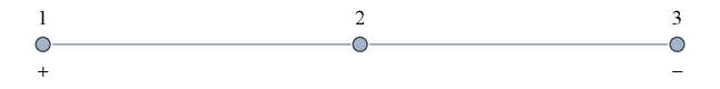
Figure 2: $A_{3}$ Dynkin diagram

The $A_{3}$ model is one of the Andrews-Baxter-Forrester models Andrews $A_{L}$ with $L=3$. In the $A_{3}$ model, the spins $a,b,c,d,...$ assigned to the sites of the lattice take heights from the set ${1,2,3}$ (from $A_{3}$ Dynkin diagram) and satisfy the adjacency condition that heights on adjacent sites must differ by $\pm 1$. In the $A_{3}$ model, the square lattice has two sublattices which can be even or odd. The heights are even on the even sublattice and odd on the odd sublattice. On the even sublattice the heights are fixed to the value 2. On the odd sublattice we identify the state $a=1$ with the usual $+$ Ising state and $a=3$ with the usual $-$ Ising state. From the $A_{3}$ Dynkin diagram (Fig. 2) we get the allowed face configurations (see Fig. 3).

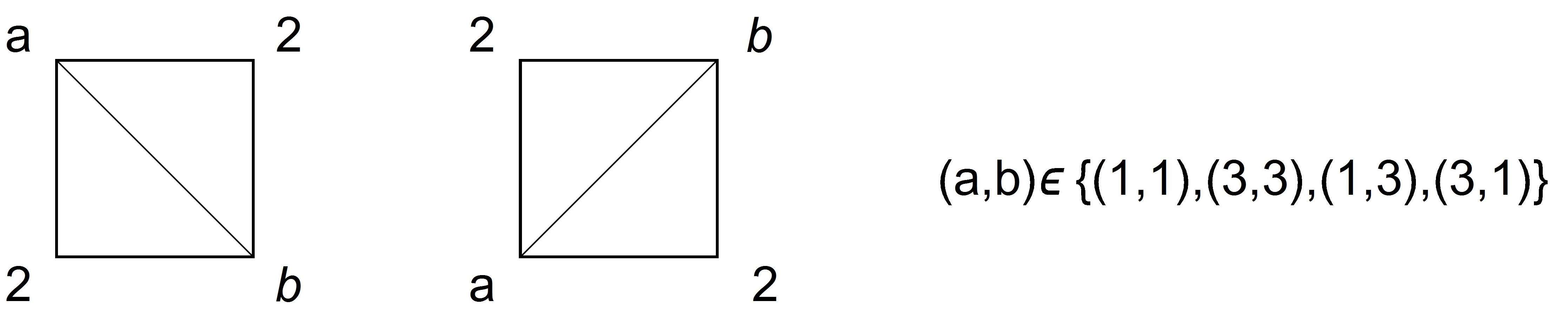
Figure 3: Allowed face configurations

We can calculate the weights of these faces by inserting the respective parameters in equation (27). Thus we get

$$W\left(\begin{array}[]{cc|}1&2\\ 2&1\end{array}\;u\right)=W\left(\begin{array}[]{cc|}3&2\\ 2&3\end{array}\;u\right)=\sqrt{2}\sin{\left(u+\frac{\pi}{4}\right)}$$ (38)

$$W\left(\begin{array}[]{cc|}3&2\\ 2&1\end{array}\;u\right)=W\left(\begin{array}[]{cc|}1&2\\ 2&3\end{array}\;u\right)=\sqrt{2}\cos{\left(u+\frac{\pi}{4}\right)}$$ (43)

$$W\left(\begin{array}[]{cc|}2&1\\ 1&2\end{array}\;u\right)=W\left(\begin{array}[]{cc|}2&3\\ 3&2\end{array}\;u\right)=\cos{\left(u\right)}$$ (48)

$$W\left(\begin{array}[]{cc|}2&3\\ 1&2\end{array}\;u\right)=W\left(\begin{array}[]{cc|}2&1\\ 3&2\end{array}\;u\right)=\sin{\left(u\right)}.$$ (53)

Obviously one can construct two kinds of transfer matrix (see Fig. 4).

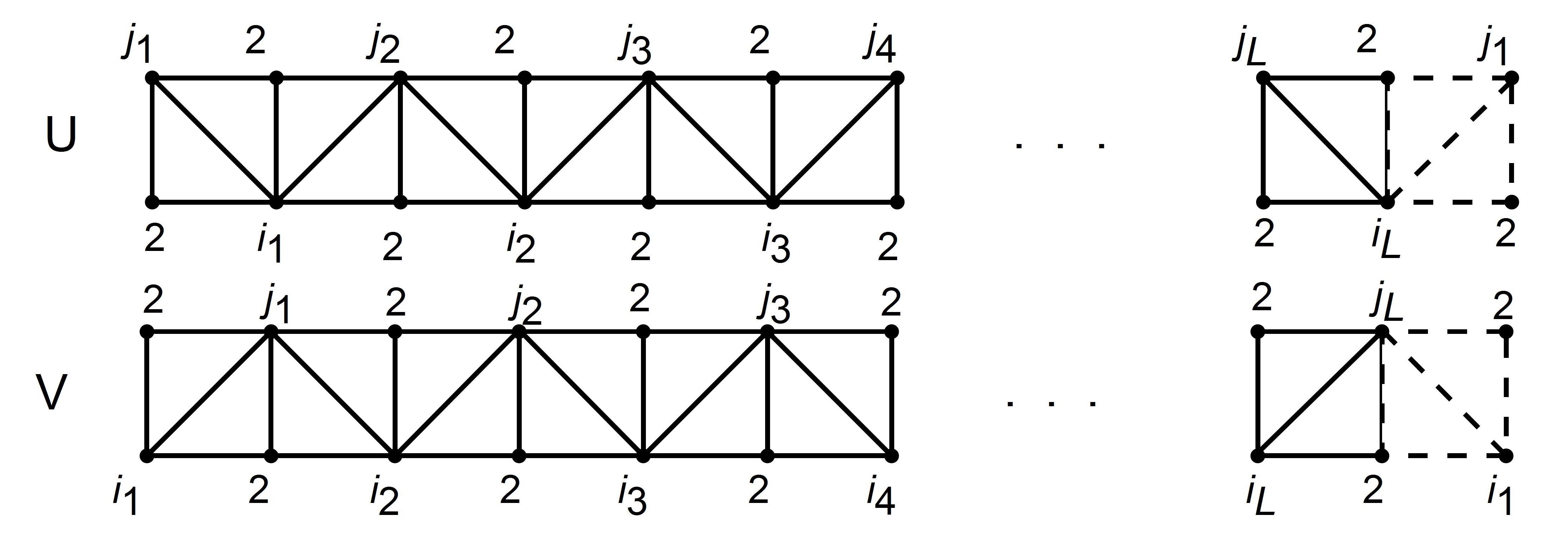
Figure 4: $U$ and $V$ transfer matrices. The rows of the transfer matrices consist of $2L-1$ regular faces followed by single seams. Single seams are represented by dashed lines. The indices $i_{k}$, $j_{k}$ take values $1$ or $3$.

Here the rows consist of $2L-1$ usual faces followed by single seams (depicted in red). The indices $i_{k}$, $j_{k}$ take values $1$ or $3$. They are ($2^{L}\times 2^{L}$) square matrices. Our boundary conditions are given with seams $(r,s)=(1,2)$, which for the $A_{3}$ model (Ising model) have the following weights Pearce2001

$$W^{(1,2)}\left(\begin{array}[]{cc}d&c\\ a&b\end{array}\right)=ie^{i\frac{\pi}{8}}\delta_{ac}-ie^{-i\frac{\pi}{8}}\frac{\sqrt{\psi_{a}\psi_{c}}}{\psi_{b}}\delta_{bd}.$$ (56)

Thus we get

$$W^{(1,2)}\begin{pmatrix}1&2\\ 2&1\end{pmatrix}=W^{(1,2)}\begin{pmatrix}3&2\\ 2&3\end{pmatrix} = ie^{i\frac{\pi}{8}}-\sqrt{2}ie^{-i\frac{\pi}{8}}$$

$$W^{(1,2)}\begin{pmatrix}3&2\\ 2&1\end{pmatrix}=W^{(1,2)}\begin{pmatrix}1&2\\ 2&3\end{pmatrix} = ie^{i\frac{\pi}{8}}$$ (57)

$$W^{(1,2)}\begin{pmatrix}2&1\\ 1&2\end{pmatrix}=W^{(1,2)}\begin{pmatrix}2&3\\ 3&2\end{pmatrix} = ie^{i\frac{\pi}{8}}-\frac{ie^{-i\frac{\pi}{8}}}{\sqrt{2}}$$

$$W^{(1,2)}\begin{pmatrix}2&3\\ 1&2\end{pmatrix}=W^{(1,2)}\begin{pmatrix}2&1\\ 3&2\end{pmatrix} = -\frac{ie^{-i\frac{\pi}{8}}}{\sqrt{2}}$$ (58)

Note that the (1,2) seam weights are complex and since the defect line can be interpreted in terms of modified bonds $J^{\prime}$ and $K^{\prime}$ it means that bonds $J^{\prime}$ and $K^{\prime}$ may be complex. In terms of these quantities we can construct the double row transfer matrix $U(u)V(v)$ (see Fig. 5).

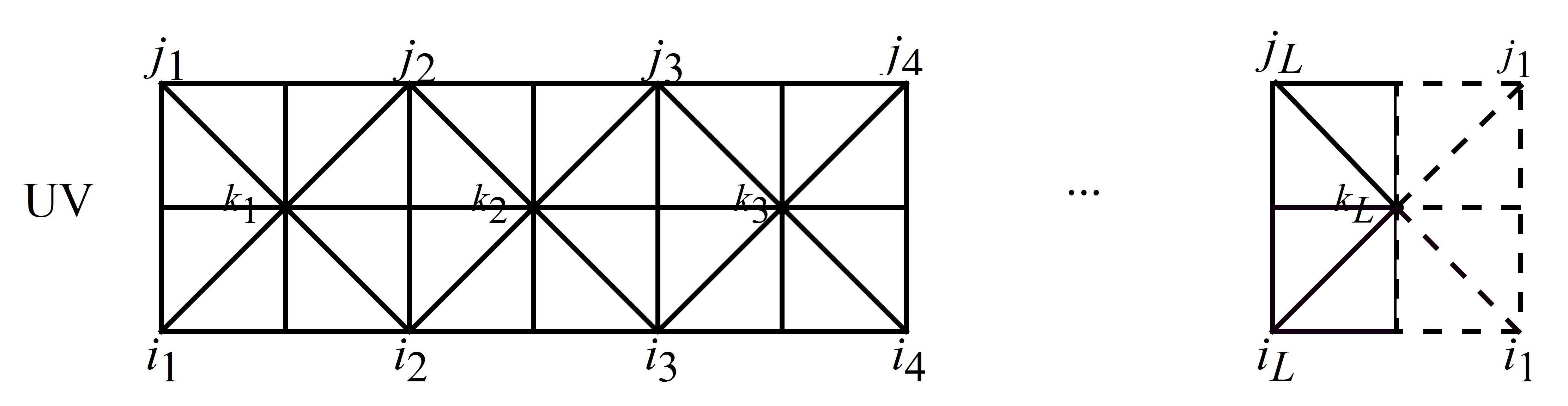
Figure 5: The $UV$ double row transfer matrix consists of $L-1$ blocks and the last dashed block.

Where $i_{a}$, $j_{a}$, $k_{a}$ take values ${1,3}$ ($a=1,...L$), and over the variables $k_{1}$, $k_{2}$,$...$, $k_{L}$ a summation is performed. On other vertexes assume non-fluctuating heights equal to $2$. The double row transfer matrix consists of $L-1$ blue blocks and the last blue-red block which we denote by $G(u,v)$ and $S(u,v)$ respectively. In terms of elemental Boltzmann weights Eqs. (38), (48), (3), (3) we get

$$G\left(\begin{array}[]{cc|c}j_{a}&j_{a+1}&u\\ i_{a}&i_{a+1}&v\end{array}\right)=\sum_{k_{a}={1,3}}W\left(\begin{array}[]{cc|}j_{a}&2\\ 2&k_{a}\end{array}\;u\right)W\left(\begin{array}[]{cc|}2&j_{a+1}\\ k_{a}&2\end{array}\;u\right)W\left(\begin{array}[]{cc|}2&k_{a}\\ i_{a}&2\end{array}\;v\right)W\left(\begin{array}[]{cc|}k_{a}&2\\ 2&i_{a+1}\end{array}\;v\right)$$ (69)

$$S\left(\begin{array}[]{cc|c}j_{L}&j_{1}&u\\ i_{L}&i_{1}&v\end{array}\right)=\sum_{k_{L}={1,3}}W\left(\begin{array}[]{cc|}j_{L}&2\\ 2&k_{L}\end{array}\;u\right)W^{(1,2)}\begin{pmatrix}2&j_{1}\\ k_{L}&2\end{pmatrix}W\left(\begin{array}[]{cc|}2&k_{L}\\ i_{L}&2\end{array}\;v\right)W^{(1,2)}\begin{pmatrix}k_{L}&2\\ 2&i_{1}\end{pmatrix}.$$ (76)

For the matrix elements of the transfer matrix $T(u,v)=U(u)V(v)$ we have

$$T^{j_{1}\;j_{2}\;j_{3}\cdots j_{L}}_{{i_{1}\;i_{2}\;i_{3}\cdots i_{L}}}(u,v)=G\left(\begin{array}[]{cc|c}j_{1}&j_{2}&u\\ i_{1}&i_{2}&v\end{array}\right)G\left(\begin{array}[]{cc|c}j_{2}&j_{3}&u\\ i_{2}&i_{3}&v\end{array}\right)...S\left(\begin{array}[]{cc|c}j_{L}&j_{1}&u\\ i_{L}&i_{1}&v\end{array}\right)$$ (84)

In what follows we will need the weights $G(u,u+\frac{\pi}{4})$ and $S(u,u+\frac{\pi}{4})$. An elementary calculation ensures that

$$G\left(\begin{array}[]{cc}1&1\\ 1&1\end{array}\right)=G\left(\begin{array}[]{cc}1&3\\ 1&3\end{array}\right)=G\left(\begin{array}[]{cc}3&1\\ 3&1\end{array}\right)=G\left(\begin{array}[]{cc}3&3\\ 3&3\end{array}\right)=\cos^{2}(2u)$$ (93)

$$G\left(\begin{array}[]{cc}1&1\\ 3&3\end{array}\right)=G\left(\begin{array}[]{cc}3&3\\ 1&1\end{array}\right)=-\sin^{2}(2u)$$ (98)

$$G\left(\begin{array}[]{cc}1&3\\ 3&1\end{array}\right)=G\left(\begin{array}[]{cc}3&1\\ 1&3\end{array}\right)=\sin^{2}(2u)$$ (103)

$$G\left(\begin{array}[]{cc}1&1\\ 1&3\end{array}\right)=G\left(\begin{array}[]{cc}1&3\\ 1&1\end{array}\right)=G\left(\begin{array}[]{cc}3&1\\ 3&3\end{array}\right)=G\left(\begin{array}[]{cc}3&3\\ 3&1\end{array}\right)=0$$ (112)

$$G\left(\begin{array}[]{cc}1&1\\ 3&1\end{array}\right)=G\left(\begin{array}[]{cc}3&3\\ 1&3\end{array}\right)=\cos(2u)+\sin(2u)$$ (117)

$$G\left(\begin{array}[]{cc}1&3\\ 3&3\end{array}\right)=G\left(\begin{array}[]{cc}3&1\\ 1&1\end{array}\right)=\cos(2u)-\sin(2u)$$ (122)

$$S\left(\begin{array}[]{cc}1&1\\ 1&1\end{array}\right)=S\left(\begin{array}[]{cc}1&3\\ 1&3\end{array}\right)=S\left(\begin{array}[]{cc}3&1\\ 3&1\end{array}\right)=S\left(\begin{array}[]{cc}3&3\\ 3&3\end{array}\right)=\cos(2u)$$ (131)

$$S\left(\begin{array}[]{cc}1&1\\ 3&3\end{array}\right)=S\left(\begin{array}[]{cc}3&3\\ 1&1\end{array}\right)=-i\sin(2u)$$ (136)

$$S\left(\begin{array}[]{cc}1&3\\ 3&1\end{array}\right)=S\left(\begin{array}[]{cc}3&1\\ 1&3\end{array}\right)=i\sin(2u)$$ (141)

$$S\left(\begin{array}[]{cc}1&1\\ 1&3\end{array}\right)=S\left(\begin{array}[]{cc}1&3\\ 1&1\end{array}\right)=S\left(\begin{array}[]{cc}3&1\\ 3&3\end{array}\right)=S\left(\begin{array}[]{cc}3&3\\ 3&1\end{array}\right)=0$$ (150)

$$S\left(\begin{array}[]{cc}1&1\\ 3&1\end{array}\right)=S\left(\begin{array}[]{cc}3&3\\ 1&3\end{array}\right)=S\left(\begin{array}[]{cc}1&3\\ 3&3\end{array}\right)=S\left(\begin{array}[]{cc}3&1\\ 1&1\end{array}\right)=1.$$ (159)

It follows from Eq. (93) that at the special point $v=u+\frac{\pi}{4}$ the only nonzero elements of the transfer matrix are

$$T^{j_{1}\;j_{2}\;j_{3}\cdots j_{L}}_{{j_{1}\;j_{2}\;j_{3}\cdots j_{L}}}\left(u,u+\frac{\pi}{4}\right)=\cos\left(2u\right)^{2L-1}$$

$$T^{j_{1}\;j_{2}\;j_{3}\cdots j_{L}}_{{\tilde{j}_{1}\;\tilde{j}_{2}\;\tilde{j}_{3}\cdots\tilde{j}_{L}}}\left(u,u+\frac{\pi}{4}\right)=i\left(-1\right)^{L}\sin\left(2u\right)^{2L-1}$$ (160)

where $\tilde{j}_{a}=3$ if $j_{a}=1$ and $\tilde{j}_{a}=1$ if $j_{a}=3$.

Thus the double row transfer matrix $U(u)V(v)$ satisfies the functional equation

$$U(u)V\left(u+\frac{\pi}{4}\right)=\cos\left(2u\right)^{2L-1}I+i\left(-1\right)^{L}\sin\left(2u\right)^{2L-1}R,$$ (161)

where $I$ is the Identity matrix, and R is a square matrix with anti-diagonal entries equal to 1 with remaining entries $0$ (both are ($2^{L}\times 2^{L}$) matrices).

4 Calculation of the Eigenvalues

Let us introduce the matrix $P(u)$

$$P(u)=\begin{pmatrix}0&V(u)\\ U(u)&0\end{pmatrix}.$$ (162)

It is easy to check that $U^{\dagger}(u)U(u)=V(u)V^{\dagger}(u)$ and, $U(u)U^{\dagger}(u)=V^{\dagger}(u)V(u)$ from which we deduce that the Matrix $P(u)$ is normal i.e. $P(u)P^{\dagger}(u)=P^{\dagger}(u)P(u)$ so that $P(u)$ is diagonalizable. Let $\Lambda(u)$ be the eigenvalue and $\begin{pmatrix}x_{1}\\ x_{2}\end{pmatrix}$ the eigenvector of $P(u)$;

$$P(u)\begin{pmatrix}x_{1}\\ x_{2}\end{pmatrix}=\begin{pmatrix}0&V(u)\\ U(u)&0\end{pmatrix}\begin{pmatrix}x_{1}\\ x_{2}\end{pmatrix}=\begin{pmatrix}V(u)x_{2}\\ U(u)x_{1}\end{pmatrix}=\Lambda(u)\begin{pmatrix}x_{1}\\ x_{2}\end{pmatrix}.$$ (163)

Evidently

$$U(u)V(v)x_{2}=\Lambda(v)U(u)x_{1}=\Lambda(u)\Lambda(v)x_{2}$$

$$V(v)U(u)x_{1}=\Lambda(u)V(v)x_{2}=\Lambda(u)\Lambda(v)x_{1}.$$ (164)

Since $R^{2}=1$, the eigenvalues of $R$ are $r=\pm 1$. By acting both sides of the Eq. (161) on the vector $x_{2}$ we get

$$\Lambda\left(u\right)\Lambda\left(u+\frac{\pi}{4}\right) = \left(\cos 2u\right)^{2L-1}+ir\left(-1\right)^{L}\left(\sin 2u\right)^{2L-1}$$ (165)

$$= \left(\cos 2u\right)^{2L-1}-r\left(i\sin 2u\right)^{2L-1}\qquad$$

$$= \left(\frac{e^{2iu}+e^{-2iu}}{2}\right)^{2L-1}-r\left(\frac{e^{2iu}-e^{-2iu}}{2}\right)^{2L-1}.$$

Let us examine the case $r=-1$ (to obtain the eigenvalues corresponding to $r=+1$, one should simply take the complex conjugates of the eigenvalues of the case $r=-1$). Changing variable from $u$ to $x\equiv e^{2iu}$ and noting that if $u\rightarrow u+\frac{\pi}{4}$ then $x\rightarrow ix$ we can obtain from Eq. (165) that

$$\Lambda\left(x\right)\Lambda\left(ix\right) = (2x)^{-(2L-1)}\left[(x^{2}+1)^{2L-1}+(x^{2}-1)^{2L-1}\right]$$ (166)

To factorize the r.h.s. of Eq. (166) we need to find the $(2L-1)$ solutions of

$$t^{2L-1}+(t-2)^{2L-1}=0,$$ (167)

where $t\equiv x^{2}+1$. The solutions $t_{k}$ for $k=1,2,...,2L-1$ can be expressed through the $2L-1$ roots of $(-1)$ and are

$$t_{k}=-\frac{2e^{\frac{i\pi(2k-1)}{2L-1}}}{1-e^{\frac{i\pi(2k-1)}{2L-1}}}.$$ (168)

Then we obtain

$$t^{2L-1}+(t-2)^{2L-1}=\prod_{k=1}^{2L-1}(t-t_{k})$$

which means that

$$\Lambda\left(x\right)\Lambda\left(ix\right) = 2^{2(1-L)}x^{-(2L-1)}\prod_{k=1}^{2L-1}\left(x^{2}-i\cot\left(\frac{\pi(2k-1)}{2(2L-1)}\right)\right).$$ (169)

Splitting this product into two parts,

$$\prod_{k=1}^{2L-1}F(k)=\prod_{k=1}^{L-1}F(k)\prod_{k=L}^{2L-1}F(k),$$ (170)

then shifting the index in the second part as $k=2L-k$, the Eq. (169) may be expressed as

$$\Lambda\left(x\right)\Lambda\left(ix\right) = 2^{2(1-L)}x^{-(2L-1)}x^{2}\prod_{k=1}^{L-1}\left(x^{2}-i\cot\left(\frac{\pi(2k-1)}{2(2L-1)}\right)\right)\left(x^{2}+i\cot\left(\frac{\pi(2k-1)}{2(2L-1)}\right)\right).$$

Let us replace $x^{2}\to-(ix)^{2}$ in the first factor of the product in Eq. (LABEL:Lamb2). We obtain

$$\Lambda\left(x\right)\Lambda\left(ix\right) = \left(2^{-L+1}\right)^{2}(x)^{-L+\frac{3}{2}}(ix)^{-L+\frac{3}{2}}\left(i^{\frac{3}{2}L-\frac{7}{4}}\right)^{2}$$ (172)

$$\prod_{k=1}^{L-1}\left(x^{2}+i\cot\frac{\pi(2k-1)}{2(2L-1)}\right)\left((ix)^{2}+i\cot\frac{\pi(2k-1)}{2(2L-1)}\right).$$

Let us now replace $x^{2}\to-(ix)^{2}$ in the second factor of the product in Eq. (LABEL:Lamb2). We obtain another equivalent representation of $\Lambda\left(x\right)\Lambda\left(ix\right)$:

$$\Lambda\left(x\right)\Lambda\left(ix\right) = \left(2^{-L+1}\right)^{2}(x)^{-L+\frac{3}{2}}(ix)^{-L+\frac{3}{2}}\left(i^{\frac{3}{2}L-\frac{7}{4}}\right)^{2}$$ (173)

$$\prod_{k=1}^{L-1}\left(x^{2}-i\cot\frac{\pi(2k-1)}{2(2L-1)}\right)\left((ix)^{2}-i\cot\frac{\pi(2k-1)}{2(2L-1)}\right)$$

From Eqs. (172) and (173) we can see that $\Lambda\left(x\right)\Lambda\left(ix\right)$ can be written as

$$\Lambda\left(x\right)\Lambda\left(ix\right) = \left(2^{-L+1}\right)^{2}(x)^{-L+\frac{3}{2}}(ix)^{-L+\frac{3}{2}}\left(i^{\frac{3}{2}L-\frac{7}{4}}\right)^{2}$$ (174)

$$\prod_{k=1}^{L-1}\left(x^{2}+i\mu_{k}\cot\frac{\pi(2k-1)}{2(2L-1)}\right)\left((ix)^{2}+i\mu_{k}\cot\frac{\pi(2k-1)}{2(2L-1)}\right)$$

where $\mu_{k}=\pm 1$ for all $k$. Now, it is easy to see from Eq. (174) that

$$\Lambda(x)=\varepsilon\,2^{-L+1}i^{\frac{3}{2}L-\frac{7}{4}}x^{-L+\frac{3}{2}}\prod_{k=1}^{L-1}\left(x^{2}+i\mu_{k}\cot\frac{\pi(2k-1)}{2(2L-1)}\right)$$ (175)

where $\varepsilon=\pm 1$. For the eigenvalues of the two row transfer matrices $UV$ of the twisted Ising model we get

$$\Lambda^{2}(u)=2^{-2L+2}\>i^{-L+\frac{1}{2}}\>e^{-2iu(2L-3)}\>\prod_{k=1}^{L-1}\left(e^{i4u}+i\mu_{k}\cot\frac{\pi(2k-1)}{2(2L-1)}\right)^{2}$$ (176)

in which $\mu_{k}=\pm 1$ can be chosen arbitrarily so we have $2^{L-1}$ eigenvalues. The remaining eigenvalues can be found by taking the complex conjugate of Eq. (176). Altogether we get $2^{L}$ eigenvalues. Thus we have obtained all $2^{L}$ eigenvalues of the two row transfer matrices $U(u)V(u)$. Let us denote the eigenvalues of the two row transfer matrices $U(u)V(u)$ by $\lambda(u)$, which is equal to

$$\lambda(u)=\Lambda^{2}(u).$$

Using the identity $\prod_{k=1}^{L-1}\sin^{2}\frac{\pi(2k-1)}{2(2L-1)}=2^{-2L+2}$ we can get a new form of Eq. (176)

$$\lambda=e^{2i\left(u-\frac{\pi}{8}\right)}\prod_{k=1}^{L-1}\left(e^{2i\left(u-\frac{\pi}{8}\right)}\sin\left(\frac{\pi(2k-1)}{2(2L-1)}\right)+\mu_{k}e^{-2i\left(u-\frac{\pi}{8}\right)}\cos\left(\frac{\pi(2k-1)}{2(2L-1)}\right)\right)^{2}.$$ (177)

Since $\lambda$ is complex quantity, we can represent it as

$$\lambda=|\lambda|\exp{(i\theta)}.$$

From Eq. (177) one can easily obtain the following expressions for the absolute value of the eigenvalue $|\lambda|$ and the argument $\theta$

$$\left|\lambda\right| = \prod_{k=1}^{L-1}\left[1+\mu_{k}\sin(4u)\sin\left(\frac{\pi(2k-1)}{2L-1}\right)\right],$$ (178)

$$\theta = 2u-\frac{\pi}{4}+\sum_{k=1}^{L-1}\arctan{\frac{\cos(4u)\cos{\left(\frac{\pi(2k-1)}{2L-1}\right)}}{\sin(4u)+\mu_{k}\sin\left(\frac{\pi(2k-1)}{2L-1}\right)}}.$$ (179)

Let us now consider the largest eigenvalue $\lambda_{0}$, which corresponds to the case when all $\mu_{k}=1$. For the absolute value of the largest eigenvalue $|\lambda_{0}|$ we obtain

$$\left|\lambda_{0}\right| = \prod_{k=1}^{L-1}\left[1+\sin(4u)\sin\left(\frac{\pi(2k-1)}{2L-1}\right)\right]$$

$$= \prod_{k=1}^{L-1}\left[1+\sin(4u)\sin\left(\frac{2\pi k}{2L-1}\right)\right]$$

$$= \prod_{k=0}^{L-1}\left[1+\sin(4u)\sin\left(\frac{\pi k}{2L-1}\right)\right].$$

The product $\prod_{k=0}^{2L-2}\left[1+\sin(4u)\sin\left(\frac{\pi k}{2L-1}\right)\right]$ can be expressed as

$$\prod_{k=0}^{2L-2}\left[1+\sin(4u)\sin\left(\frac{\pi k}{2L-1}\right)\right]=\prod_{k=0}^{L-1}\left[1+\sin(4u)\sin\left(\frac{\pi k}{2L-1}\right)\right]^{2}.$$ (181)

Then the absolute value of $\lambda_{0}$ can be written in the form

$$\left|\lambda_{0}\right| = \sqrt{\prod_{k=0}^{2L-2}\left[1+\sin(4u)\sin\left(\frac{\pi k}{2L-1}\right)\right]}.$$

The argument $\theta_{0}$ of the largest eigenvalue $\lambda_{0}$ is given by

$$\theta_{0}=2u-\frac{\pi}{4}+\sum_{k=1}^{L-1}\arctan{\frac{\cos(4u)\cos{\left(\frac{\pi(2k-1)}{2L-1}\right)}}{\sin(4u)+\sin\left(\frac{\pi(2k-1)}{2L-1}\right)}}.$$ (182)

Let us change variable $k$ as $k\to L-k$. Then the argument $\theta_{0}$ given by Eq. (182) can be transformed to the form

$$\theta_{0}=2u-\frac{\pi}{4}-\sum_{k=1}^{L-1}\arctan{\frac{\cos(4u)\cos{\left(\frac{2\pi k}{2L-1}\right)}}{\sin(4u)+\sin\left(\frac{2\pi k}{2L-1}\right)}}.$$ (183)

The sum over $k$ in Eq. (183) can be extended up to $2L-2$ as

$$\theta_{0} = 2u-\frac{\pi}{4}+\frac{1}{2}\sum_{k=1}^{2L-2}(-1)^{k+1}\arctan{\frac{\cos(4u)\cos{\left(\frac{\pi k}{2L-1}\right)}}{\sin(4u)+\sin\left(\frac{\pi k}{2L-1}\right)}}$$ (184)

$$= \frac{1}{2}\sum_{k=0}^{2L-2}(-1)^{k+1}\arctan{\frac{\cos(4u)\cos{\left(\frac{\pi k}{2L-1}\right)}}{\sin(4u)+\sin\left(\frac{\pi k}{2L-1}\right)}}.$$ (185)

In the last step we have use the fact that $\frac{1}{2}\arctan{\cot{(4u)}}=\frac{\pi}{4}-2u$.

The derivation of the asymptotic expansion of $\log\lambda_{0}=\log\left|\lambda_{0}\right|+i\theta_{0}$ can be divided to two parts. First, with the help of the Euler-Maclaurin summation formula (see Eq. (308) in appendix A) we can derive the asymptotic expansion of the logarithm of the absolute value of $\lambda_{0}$

$$\log\left|\lambda_{0}\right| = \frac{1}{2}\sum_{k=0}^{2L-2}\log\left[1+\sin(4u)\sin\left(\frac{\pi k}{2L-1}\right)\right]$$ (186)

$$= -f_{\rm{bulk}}(2L-1)-2\sum_{k=0}^{\infty}\frac{B_{2k+2}f^{(2k+1)}(0)}{(2k+2)!}\left(\frac{\pi}{2L-1}\right)^{2k+1}$$

$$= -f_{\rm{bulk}}(2L-1)-\frac{\pi\sin(4u)}{12}\frac{1}{2L-1}-\frac{\pi^{3}\sin(4u)\cos(8u)}{720(2L-1)^{3}}+...$$ (187)

where $f(x)$ is given by

$$f(x)=\frac{1}{2}\log\left[1+\sin(4u)\sin x\right]$$ (188)

and $f_{\rm{bulk}}$ is given by

$$f_{\rm{bulk}}=-\frac{1}{\pi}\int_{0}^{\pi}f(x)dx=-\frac{1}{2\pi}\int_{0}^{\pi}\log\left[1+\sin(4u)\sin x\right]dx.$$ (189)

Now with the help of the Boole summation formula (see Eq. (313) in appendix A) the asymptotic expansion of the argument $\theta_{0}$ can be written in the form

$$\theta_{0} = \frac{1}{2}\sum_{k=0}^{2L-2}(-1)^{k+1}\arctan{\frac{\cos(4u)\cos{\left(\frac{\pi k}{(2L-1)}\right)}}{\sin(4u)+\sin\left(\frac{\pi k}{(2L-1)}\right)}}$$ (190)

$$= -\frac{1}{2}\sum_{n=0}^{\infty}\frac{E_{2n+1}(0)}{(2n+1)!}\left[g^{(2n+1)}(\pi)+g^{(2n+1)}(0)\right]\left(\frac{\pi}{2L-1}\right)^{2n+1}$$

where function $g(x)$ is given by

$$g(x)=\frac{1}{2}\arctan{\frac{\cos(4u)\cos x}{\sin(4u)+\sin x}}.$$ (191)

Since the function $g(x)$ obeys the symmetry $g(x)=-g(\pi-x)$, the derivatives of the function $g(x)$ at the points zero and $\pi$ are related to each other as

$$g^{(2k+1)}(0) = g^{(2k+1)}(\pi),\qquad\qquad k=0,1,2,...$$ (192)

$$g^{(2k)}(0) = -g^{(2k)}(\pi),\qquad\qquad k=0,1,2,....$$ (193)

Using Eq. (192) the asymptotic expansion of the argument of $\lambda$ can finally be written in the form

$$\theta_{0} = -\sum_{n=0}^{\infty}\frac{E_{2n+1}(0)g^{(2n+1)}(0)}{(2n+1)!}\left(\frac{\pi}{2L-1}\right)^{2n+1}$$ (194)

$$= -\frac{\pi\cos{(4u)}}{4(2L-1)}+\frac{\pi^{3}\sin(4u)\sin(8u)}{48(2L-1)^{3}}+....$$ (195)

Thus the leading finite-size corrections to the ground state energies ${\cal E}_{0}=\frac{\sqrt{2}}{2}{\bf E}_{0}=-\frac{\sqrt{2}}{2}\log\lambda_{0}$ take the form

$${\cal E}_{0}=-\frac{\sqrt{2}}{2}\log{\lambda_{0}} = f_{\rm{bulk}}\frac{\sqrt{2}}{2}(2L-1)+\frac{2\sqrt{2}\pi}{2L-1}\left(\frac{1}{48}\sin(4u)+\frac{i}{16}\cos(4u)\right)+O\left(\frac{1}{2L-1}\right).$$

The leading finite-size corrections to the ground state energies ${\cal E}_{0}$ given by Eq. (24) for the Ising model with $c=1/2$ and $g=4$ take the form

$${\cal E}_{0} = L_{x}f_{\rm{bulk}}+\frac{2\pi}{L_{x}}\left[\left(-\frac{1}{24}+\Delta+\bar{\Delta}\right)\sin(4u)+i(\Delta-\bar{\Delta})\cos(4u)\right]+O\left(\frac{1}{L_{x}}\right)$$ (197)

$$= L_{x}f_{\rm{bulk}}+\frac{2\pi i}{L_{x}}\left[\left(-\frac{1}{48}+\Delta\right)e^{-i4u}-\left(-\frac{1}{48}+\bar{\Delta}\right)e^{i4u}\right]+O\left(\frac{1}{L_{x}}\right).$$ (198)

Compare Eqs. (LABEL:E0Ising) and (197) for $L_{x}=\sqrt{2}(L-1/2)$ we can see that $\Delta=1/16$ and $\bar{\Delta}=0$. Thus we have shown that duality twisted boundary conditions with $\left(\Delta,\bar{\Delta}\right)=\left(\frac{1}{16},0\right)$ correspond to the boundary conditions with seam $(r,s)=(1,2)$.

Let us now consider the other eigenvalues given by Eq. (177), which correspond to some combination of the $\{\mu_{k}\}=(\mu_{1},\mu_{2},...,\mu_{L-1})$. Denote by $\lambda_{\{p\}}$ the eigenvalue given by Eq. (177) with $\mu_{p}=-1$ and the other $\mu_{k}$ have value $\mu_{k}=+1$. The first exited state corresponds to the second largest eigenvalues $\lambda_{1}=\lambda_{\{1\}}$, and the second exited state corresponds to the third largest eigenvalue $\lambda_{2}=\lambda_{\{L-1\}}$. It is easy to show that

$$\lambda_{\{p\}} = \lambda_{0}\left[\frac{\exp[2i\left(u-\frac{\pi}{8}\right)]\sin\left(\frac{\pi(2p-1)}{4L-2}\right)-\exp[-2i\left(u-\frac{\pi}{8}\right)]\cos\left(\frac{\pi(2p-1)}{4L-2}\right)}{\exp[2i\left(u-\frac{\pi}{8}\right)]\sin\left(\frac{\pi(2p-1)}{4L-2}\right)+\exp[-2i\left(u-\frac{\pi}{8}\right)]\cos\left(\frac{\pi(2p-1)}{4L-2}\right)}\right]^{2}$$ (199)

$$= \lambda_{0}A_{p}e^{i\phi_{p}}$$ (200)

where $A_{p}$ and $\phi_{p}$ are given by

$$\log A_{p} = \log\frac{1-\sin(4u)\sin\left(\frac{\pi(2p-1)}{2L-1}\right)}{1+\sin(4u)\sin\left(\frac{\pi(2p-1)}{2L-1}\right)}=-4\sum_{n=0}^{\infty}\frac{(2p-1)^{2n+1}f^{(2n+1)}(0)}{(2n+1)!}\left(\frac{\pi}{2L-1}\right)^{2n+1}$$ (201)

$$\phi_{p} = 2\arctan\left[\cos(4u)\tan\left(\frac{\pi(2p-1)}{2L-1}\right)\right]=-4\sum_{n=0}^{\infty}\frac{(2p-1)^{2n+1}g^{(2n+1)}(0)}{(2n+1)!}\left(\frac{\pi}{2L-1}\right)^{2n+1}$$ (202)

For values of $p$ close to $L$ its convenient consider instead of Eq. (200) the expressions

$$\lambda_{\{L-p\}} = \lambda_{0}A_{L-p}e^{i\phi_{L-p}}.$$ (203)

From Eqs. (201) and (202) one can easily obtain the expressions for the $A_{L-p}$ and $\phi_{L-p}$:

$$\log A_{L-p} = \log\frac{1-\sin(4u)\sin\left(\frac{2p\pi}{2L-1}\right)}{1+\sin(4u)\sin\left(\frac{2p\pi}{2L-1}\right)}=-4\sum_{n=0}^{\infty}\frac{(2p)^{2n+1}f^{(2n+1)}(0)}{(2n+1)!}\left(\frac{\pi}{2L-1}\right)^{2n+1}$$ (204)

$$\phi_{L-p} = -2\arctan\left[\cos(4u)\tan\left(\frac{2p\pi}{2L-1}\right)\right]=4\sum_{n=0}^{\infty}\frac{(2p)^{2n+1}g^{(2n+1)}(0)}{(2n+1)!}\left(\frac{\pi}{2L-1}\right)^{2n+1}.$$ (205)

The asymptotic expansions of $\log\lambda_{\{p\}}$ and $\log\lambda_{\{L-p\}}$ can be written by using Eqs. (179), (186), (201), (202), (204) and (205) as

$$-\log\lambda_{\{p\}} = f_{\rm{bulk}}(2L-1)+2\sum_{n=0}^{\infty}\left(\frac{B_{2n+2}}{2n+2}+2(2p-1)^{2n+1}\right)\frac{f^{(2n+1)}(0)}{(2n+1)!}\left(\frac{\pi}{2L-1}\right)^{2n+1}$$ (206)

$$+i\sum_{n=0}^{\infty}\left(E_{2n+1}(0)+4(2p-1)^{2n+1}\right)\frac{g^{(2n+1)}(0)}{(2n+1)!}\left(\frac{\pi}{2L-1}\right)^{2n+1}$$

$$-\log\lambda_{\{L-p\}} = f_{\rm{bulk}}(2L-1)+2\sum_{n=0}^{\infty}\left(\frac{B_{2n+2}}{2n+2}+2(2p)^{2n+1}\right)\frac{f^{(2n+1)}(0)}{(2n+1)!}\left(\frac{\pi}{2L-1}\right)^{2n+1}$$ (207)

$$+i\sum_{n=0}^{\infty}\left(E_{2n+1}(0)-4(2p)^{2n+1}\right)\frac{g^{(2n+1)}(0)}{(2n+1)!}\left(\frac{\pi}{2L-1}\right)^{2n+1}.$$

From Eqs. (206) and (207) one can obtain the leading finite-size corrections to the exited state energies ${\cal E}_{p}=\frac{\sqrt{2}}{2}{\bf E}_{p}=-\frac{\sqrt{2}}{2}\log\lambda_{\{p\}}$ and ${\cal E}_{L-p}=\frac{\sqrt{2}}{2}{\bf E}_{L-p}=-\frac{\sqrt{2}}{2}\log\lambda_{\{L-p\}}$ in the form

$${\cal E}_{p}=-\frac{\sqrt{2}}{2}\log\lambda_{\{p\}}=L_{x}f_{\rm{bulk}}$$

$$+\frac{2\pi}{L_{x}}\left[\left(-\frac{23}{48}+p\right)\sin{(4u)}+i\left(\frac{9}{16}-p\right)\cos{(4u)}\right]+O\left[\frac{1}{L_{x}}\right]^{2}$$

$$=L_{x}f_{\rm{bulk}}+\frac{2\pi i}{L_{x}}\left[\frac{1}{24}e^{-4iu}+\left(\frac{25}{48}-p\right)e^{4iu}\right]+O\left[\frac{1}{L_{x}}\right]^{2}$$ (208)

$${\cal E}_{L-p}=-\frac{\sqrt{2}}{2}\log\lambda_{\{L-p\}}=L_{x}f_{\rm{bulk}}$$

$$+\frac{2\pi}{L_{x}}\left[\left(\frac{1}{48}+p\right)\sin(4u)+i\left(\frac{1}{16}+p\right)\cos(4u)\right]+O\left[\frac{1}{L_{x}}\right]^{2}$$

$$=L_{x}f_{\rm{bulk}}+\frac{2\pi i}{L_{x}}\left[\left(\frac{1}{24}+p\right)e^{-4iu}+\frac{1}{48}e^{4iu}\right]+O\left[\frac{1}{L_{x}}\right]^{2}$$ (209)

where $L_{x}$ is given by Eq. (16).

The leading finite-size corrections to the exited state energies ${\cal E}_{n}$ given by Eqs. (22) and (23) for the Ising model with $c=1/2$ and $g=4$ take the form

$${\cal E}_{n} = L_{x}f_{\rm{bulk}}+\frac{2\pi}{L_{x}}\left[\left(-\frac{1}{24}+\Delta+\bar{\Delta}+k_{n}+\bar{k}_{n}\right)\sin(4u)+i(\Delta-\bar{\Delta}+k_{n}-\bar{k}_{n})\cos(4u)\right]$$ (210)

$$+ O\left(\frac{1}{L_{x}}\right)$$

$$= L_{x}f_{\rm{bulk}}+\frac{2\pi i}{L_{x}}\left[\left(-\frac{1}{48}+\Delta+k_{n}\right)e^{-i4u}-\left(-\frac{1}{48}+\bar{\Delta}+\bar{k}_{n}\right)e^{i4u}\right]+O\left(\frac{1}{L_{x}}\right).$$

Now compare Eqs. (208), (209) with Eq. (210) we can see that for the exited state ${\cal E}_{p}$ we have

$$|\Delta=1/16,k_{p}=0;\bar{\Delta}=1/2,\bar{k}_{p}=p-1\rangle$$ (211)

and for the exited state ${\cal E}_{L-p}$ we have

$$|\Delta=1/16,k_{L-p}=p;\bar{\Delta}=0,\bar{k}_{L-p}=0\rangle.$$ (212)

5 Twisted partition function $Z_{(1,2)}(p)$

Now we have all the necessary information to start the calculations of partition function for the Ising model with duality-twisted boundary conditions $Z_{L_{x}L_{y}}$. For large $L_{x}$ and $L_{y}$ (always keeping the ratio $L_{y}/L_{x}$ constant) we have

$$Z_{L_{x}L_{y}}=\sum_{l}\lambda_{l}^{M}\approx e^{-L_{x}L_{y}f_{\rm{bulk}}}Z_{(1,2)}(q),$$ (213)

where $f_{\rm{bulk}}$ is the bulk free energy, $q$ is the modular parameter and $Z_{(1,2)}(q)$ is the universal conformal partition function.

Let us now find the general form of the eigenvalues with significant input in the partition function. From Eq. (178) we can see that these are eigenvalues for which almost all $\mu_{k}=1$ and some $\mu_{k}$ are allowed to take the value $-1$ only if $k\ll L$ or $L-k\ll L$. Any “significant” eigenvalue will be specified by two sets of indexes $K=\{k_{1},k_{2},\cdots,k_{m}\}$ and $\bar{K}=\{\bar{k}_{1},\bar{k}_{2},\cdots,\bar{k}_{\bar{m}}\}$, where $\bar{k}_{i}\equiv L-k_{i}$ with $k_{1}<k_{2}<k_{3}<\cdots<k_{m}\ll L$ and $\bar{k_{1}}<\bar{k_{2}}<\bar{k_{3}}<\cdots<\bar{k}_{\bar{m}}\ll L$ so that $\mu_{\bar{k}_{i}}=-1$,$\mu_{k_{i}}=-1$ and the other $\mu$’s are $+1$. From above it is easy to get

$$-\frac{\sqrt{2}}{2}\log\lambda_{K\bar{K}}=L_{x}f_{\rm{bulk}}$$

$$+\frac{2\pi i}{L_{x}}\left[\left(-\frac{c}{24}+\frac{1}{16}+\sum_{i}k_{i}\right)e^{-4iu}-\left(-\frac{c}{24}+\sum_{i}\left(\bar{k}_{i}-\frac{1}{2}\right)\right)e^{4iu}\right]+O\left[\frac{1}{N}\right]^{2}.$$ (214)

From antiholomorphic part of the Eq. (214) one can see that exited state in antiholomorphic region is correspond to the conformal state $\bar{\psi}_{-\bar{\nu}_{1}}\bar{\psi}_{-\bar{\nu}_{2}}...\bar{\psi}_{-\bar{\nu}_{n}}|0>$, where $\bar{\nu}_{i}=\bar{k}_{i}-1/2$ are half integer numbers. In particular the exited state ${\cal E}_{p}$ ($|p>$) given by Eq. (211) corresponds to the conformal state $\bar{\psi}_{-p+1/2}|0>$. It is easy to show that

$$[L_{-1}\bar{\psi}_{m}]=\left(\frac{1}{2}-m\right)\,\bar{\psi}_{m-1}$$ (215)

from which, using the fact that $L_{-1}|0>=0$ one can derive that

$$\bar{\psi}_{-p+1/2}|0>=\frac{1}{(p-1)!}[L_{-1}^{p-1}\bar{\psi}_{-1/2}]|0>=\frac{1}{(p-1)!}L_{-1}^{p-1}\bar{\psi}_{-1/2}|0>=\frac{1}{(p-1)!}L_{-1}^{p-1}|1/2>$$ (216)

Thus the state $|p>$ is the descendent conformal state $L_{-1}^{p-1}|\bar{\Delta}>$ generated by the primary field $\bar{\psi}(\bar{z})$ with conformal dimension $\bar{\Delta}=1/2$. Now from holomorphic part of the Eq. (214) one can see that exited state in holomorphic region is correspond to the conformal state $\psi_{-k_{1}}\psi_{-k_{2}}...\psi_{-k_{n}}|\sigma>$, where $|\sigma>=\sigma(0)|0>$ is the asymptotic state created by a primary field $\sigma(0)$ of the conformal dimension $\Delta=1/16$. The exited state ${\cal E}_{p}$ ($|L-p>$) given by Eq. (212) correspond to the conformal state $\psi_{-p}|\sigma>=\psi_{-p}\sigma(0)|0>$, which can be considered as descendent of the conformal state generated by product of two conformal fields $\psi(z)\sigma(0)$.

Now from Eqs. (213) and (5) we can obtain that

$$Z_{(1,2)}(q)=\sum_{K\bar{K}}q^{-\frac{c}{24}+\frac{1}{16}+\sum_{i}k_{i}}\bar{q}^{-\frac{c}{24}+\sum_{i}\left(\bar{k}_{i}-\frac{1}{2}\right)}$$ (217)

where $q$ is a modular parameter given by

$$q=e^{-\frac{2\pi iL_{y}}{L_{x}}e^{-4iu}}.$$ (218)

For further calculations it is convenient to introduce the occupation numbers $\varepsilon_{k}=\frac{1-\mu_{k}}{2}$ and $\bar{\varepsilon}_{\bar{k}}=\frac{1-\bar{\mu}_{\bar{k}}}{2}$. In terms of this quantities the universal conformal partition function Eq. (217) can be rewritten as

$$Z_{(1,2)}(q)=\sum_{\{\varepsilon\}\{\bar{\varepsilon}\}}q^{-\frac{c}{24}+\frac{1}{16}+\sum_{k}^{\infty}k\varepsilon_{k}}\bar{q}^{-\frac{c}{24}+\sum_{\bar{k}}^{\infty}\left(\bar{k}-\frac{1}{2}\right)\bar{\varepsilon}_{\bar{k}}}$$

$$=q^{-\frac{c}{24}+\frac{1}{16}}\bar{q}^{-\frac{c}{24}}\sum_{\{\varepsilon\}\{\bar{\varepsilon}\}}\prod_{k=1}^{\infty}q^{k\varepsilon_{k}}\prod_{\bar{k}=1}^{\infty}\bar{q}^{\left(\bar{k}-\frac{1}{2}\right)\bar{\varepsilon}_{\bar{k}}}$$

$$=q^{-\frac{c}{24}+\frac{1}{16}}\bar{q}^{-\frac{c}{24}}\sum_{\varepsilon_{1}\in\{0,1\}}\sum_{\varepsilon_{2}\in\{0,1\}}\cdots\sum_{\bar{\varepsilon}_{1}\in\{0,1\}}\sum_{\bar{\varepsilon}_{2}\in\{0,1\}}\cdots\prod_{k=1}^{\infty}q^{k\varepsilon_{k}}\prod_{\bar{k}=1}^{\infty}\bar{q}^{\left(\bar{k}-\frac{1}{2}\right)\bar{\varepsilon}_{\bar{k}}}$$

$$=q^{-\frac{c}{24}+\frac{1}{16}}\bar{q}^{-\frac{c}{24}}\prod_{k=1}^{\infty}\left(1+q^{k}\right)\prod_{\bar{k}=1}^{\infty}\left(1+\bar{q}^{\bar{k}-\frac{1}{2}}\right).$$ (219)

Taking into account that

$$\chi_{0}=\frac{1}{2}q^{-\frac{1}{48}}\left(\prod_{k=1}^{\infty}\left(1+q^{k-\frac{1}{2}}\right)+\prod_{k=1}^{\infty}\left(1-q^{k-\frac{1}{2}}\right)\right)$$

$$\chi_{\frac{1}{2}}=\frac{1}{2}q^{-\frac{1}{48}}\left(\prod_{k=1}^{\infty}\left(1+q^{k-\frac{1}{2}}\right)-\prod_{k=1}^{\infty}\left(1-q^{k-\frac{1}{2}}\right)\right)$$

$$\chi_{\frac{1}{16}}=q^{\frac{1}{24}}\prod_{k=1}^{\infty}\left(1+q^{k}\right),$$ (220)

and adding the conjugate part of the eigenvalue set we get

$$Z_{(1,2)}(q)=\left[\chi_{0}(q)+\chi_{\frac{1}{2}}(q)\right]^{*}\chi_{\frac{1}{16}}(q)+\left[\chi_{0}(q)+\chi_{\frac{1}{2}}(q)\right]\chi_{\frac{1}{16}}(q)^{*}.$$ (221)

Thus we have obtained analytically the universal conformal partition function for the Ising model with duality-twisted boundary conditions $Z_{(1,2)}(q)$ which confirms the numerical result of Pearce2001 .

6 Universal amplitude ratios

In this section we present the set of universal amplitude ratios for finite-size corrections of the two-dimensional Ising model on square lattices with duality-twisted boundary conditions given by Eq. (10). Let us denote the free energy per spin $f$, the inverse correlation lengths $\xi^{-1}_{p}$ and $\xi^{-1}_{L-p}$ of our critical Ising model as

$$L_{x}f = -\frac{\sqrt{2}}{2}\log\left(\left|\lambda_{0}\right|\right)$$ (222)

$$\xi^{-1}_{p} = \frac{\sqrt{2}}{2}\log\left(\left|\frac{\lambda_{0}}{\lambda_{\{p\}}}\right|\right)=-\frac{\sqrt{2}}{2}\log{A_{p}}$$ (223)

$$\xi^{-1}_{L-p} = \frac{\sqrt{2}}{2}\log\left(\left|\frac{\lambda_{0}}{\lambda_{\{L-p\}}}\right|\right)=-\frac{\sqrt{2}}{2}\log{A_{L-p}}.$$ (224)

From Eqs. (186), (201) and (204) it is clear that asymptotic expansions for the free energy per spin $f$ and the inverse correlation lengths $\xi^{-1}_{p}$ and $\xi^{-1}_{L-p}$ can be written in the forms

$$L_{x}(f-f_{\rm{bulk}}) = \sum_{k=1}^{\infty}\frac{a_{k}(p)}{L_{x}^{2k-1}}$$ (225)

$$\xi^{-1}_{p} = \sum_{k=1}^{\infty}\frac{b_{k}(p)}{L_{x}^{2k-1}}$$ (226)

$$\xi^{-1}_{L-p} = \sum_{k=1}^{\infty}\frac{c_{k}(p)}{L_{x}^{2k-1}},$$ (227)

where coefficients $a_{k}(p)$, $b_{k}(p)$ and $c_{k}(p)$ are given by

$$a_{k}(p) = \frac{\pi^{2k-1}B_{2k}}{2^{k-1}(2k)!}f^{(2k-1)}(0)$$ (228)

$$b_{k}(p) = \frac{\pi^{2k-1}(2p-1)^{2k-1}}{2^{k-2}(2k-1)!}f^{(2k-1)}(0)$$ (229)

$$c_{k}(p) = \frac{2^{k+1}\pi^{2k-1}p^{2k-1}}{(2k-1)!}f^{(2k-1)}(0).$$ (230)

The coefficients $a_{1}(p)$, $b_{1}(p)$, $c_{1}(p)$

$$a_{1}(p) = \frac{\pi}{24}\sin{y}$$ (231)

$$b_{1}(p) = (2p-1)\pi\sin{y}$$ (232)

$$c_{1}(p) = 2p\pi\sin{y}$$ (233)

are universal and related to the conformal anomaly number (c), the conformal dimensions of the ground state ($\Delta,\bar{\Delta}$), and the scaling dimensions of the $p$-th scaling fields ($x_{p},z_{p}$) of the theory in the following way

$$a_{1}(p) = 2\pi\zeta\left(-\frac{c}{12}+\Delta+\bar{\Delta}\right)$$ (234)

$$b_{1}(p) = 2\pi\zeta x_{p}$$ (235)

$$c_{1}(p) = 2\pi\zeta z_{p},$$ (236)

with $c=1/2$, $\Delta=1/16$, $\bar{\Delta}=0$, $x_{p}=p-1/2$, $z_{p}=p$ and anisotropy parameter $\zeta=\sin y$.

The coefficients $a_{k}(p)$, $b_{k}(p)$ and $c_{k}(p)$ for $k\geq 2$ are non-universal, since they depends on non-universal parameter $f^{(2k-1)}(0)$, but ratio of this coefficients are universal and given by

$$r_{p}(k)=\frac{b_{k}(p)}{a_{k}(p)} = \frac{4k(2p-1)^{2k-1}}{B_{2k}}$$ (237)

$$r_{L-p}(k)=\frac{c_{k}(p)}{a_{k}(p)} = \frac{4k(2p)^{2k-1}}{B_{2k}}.$$ (238)

Below we will show that universality of the ratios $r_{p}(k),r_{L-p}(k)$ for $k=1$ and $2$ follow from the conformal field theory.

The case for $k=1$ is trivial, since $r_{p}(1)$ and $r_{L-p}(1)$ are the ratios of universal coefficients $a_{1}(p)$, $b_{1}(p)$ and $c_{1}(p)$ and equal to

$$r_{p}(1) = 24(2p-1)$$ (239)

$$r_{L-p}(1) = 48p.$$ (240)

The case $k=2$ is non-trivial. The ratios $r_{p}(2)$ and $r_{L-p}(2)$ are given by

$$r_{p}(2) = -240(2p-1)^{3}$$ (241)

$$r_{L-p}(2) = -1920p^{3}.$$ (242)

7 Perturbative conformal field theory

The finite-size corrections to Eq. (22) can in principle be computed in perturbative conformal field theory. In general, any critical lattice Hamiltonian contains correction terms to the fixed-point Hamiltonian $H_{c}=\frac{\pi}{L_{x}}\left(L_{0}+\bar{L}_{0}-\frac{c}{12}\right)$

$$H=\zeta H_{c}+\sum_{k}g_{k}\int_{-L_{x}/2}^{L_{x}/2}\phi_{k}(v)dv,$$ (243)

where $g_{k}$ is a non-universal constant and $\phi_{k}(v)$ is a perturbating conformal field with scaling dimension $x_{k}$. Among these fields are those associated with the conformal block of the identity operator, the leading operator of which has the scaling dimension $x_{l}=4$. To first order in the perturbation, the energy gaps $({\cal E}_{n}-{\cal E}_{0})$ and the ground-state energy (${\cal E}_{0}$) can be written as

$${\cal E}_{n}-{\cal E}_{0} = \frac{2\pi}{L_{x}}\zeta x_{n}+2\pi\sum_{k}g_{k}(C_{nkn}-C_{0k0})\left(\frac{2\pi}{L_{x}}\right)^{x_{k}-1},$$

$${\cal E}_{0} = {\cal E}_{0,c}+2\pi\sum_{k}g_{k}C_{0k0}\left(\frac{2\pi}{L_{x}}\right)^{x_{k}-1},$$

where $C_{nkn}$ are universal structure constants. Note, that the ground state energy ${\cal E}_{0}$ and the energy gaps (${\cal E}_{n}-{\cal E}_{0}$) are, respectively, the quantum analogues of the free energy $f$ and inverse spin-spin correlation lengths $\xi_{n}^{-1}$; that is, $L_{x}f\Leftrightarrow{\cal E}_{0},\quad\xi_{n}^{-1}\Leftrightarrow{\cal E}_{n}-{\cal E}_{0}$.

In the case of the cylinder geometry the spectra of the Hamiltonian (243) are built by the irreducible representation $\Delta,\bar{\Delta}$ of two commuting Virasoro algebras $L_{n}$ and ${\bar{L}}_{n}$. The leading finite-size corrections ($1/L_{x}^{3}$) can be described by the Hamiltonian given by Eq. (243) with a single perturbating conformal field $\phi_{1}(v)=L_{-2}^{2}(v)+\bar{L}_{-2}^{2}(v)$ with scaling dimension $x_{1}=4$, which belongs to the tower of the identity henkel . Thus the ratio $r_{n}(2)$ are indeed universal and given by

$$r_{n}(2)=\frac{C_{n1n}-C_{010}}{C_{010}}.$$

The universal structure constants $C_{n1n}$ can be obtained from the matrix elements $\langle n|\phi_{1}(0)|n\rangle=\left({2\pi}/{L_{x}}\right)^{x_{1}}C_{n1n}$ cardy86 , which for descendent states ($L_{-1}^{n}|\Delta\rangle$) generated by primary field $\psi(z,\bar{z})$ with conformal dimension $\Delta$ have already been computed by Reinicke reinicke87 :

$$C_{n1n} = \left(\frac{c}{24}\right)^{2}+\frac{11c}{1440}+(\Delta+r)\left(\Delta-\frac{2+c}{12}+\frac{r(2\Delta+r)(5\Delta+1)}{(\Delta+1)(2\Delta+1)}\right)$$ (244)

$$+ \frac{r}{30}\left[r^{2}(5c-8)-(5c+28)\right]\delta_{\Delta,0}+(\Delta\rightarrow\bar{\Delta},r\rightarrow\bar{r}).$$

Let us consider the case $c=1/2$. For the two-dimensional Ising model with duality-twisted boundary conditions the ground state $|0\rangle$, the excited states $|p\rangle$ and $|L-p\rangle$ are given by

$$|0\rangle = |\Delta_{0}=\frac{1}{16},r=0;\bar{\Delta}_{0}=0,\bar{r}=0\rangle$$ (245)

$$|p\rangle = |\Delta_{p}=\frac{1}{16},r=0;\bar{\Delta}_{p}=\frac{1}{2},\bar{r}=p-1\rangle$$ (246)

$$|L-p\rangle = |\Delta_{L-p}=\frac{1}{16},r=p;\bar{\Delta}_{L-p}=0,\bar{r}=0\rangle.$$ (247)

Note that the excited states $|p\rangle$ can be identified as descendent states of the primary field $\psi(z)$ with conformal dimension $\bar{\Delta}=1/2$, while the excited states $|L-p\rangle$ can be identified as descendent states generated by the OPE of the primary fields $\psi(z)\sigma(0)$ where $\sigma(0)$ is the spin operator with conformal dimension $\Delta=1/16$. Thus for descendent states of the primary field the universal structure constants $C_{n1n}$ can be obtained from Eq. (244):

$$C_{010} = -\frac{7}{11520},$$ (248)

$$C_{p1p} = -\frac{7}{11520}+\frac{7(2p-1)^{3}}{48}.$$ (249)

Now the ratios $r_{p}$ are given by

$$r_{p} = \frac{C_{p1p}-C_{010}}{C_{010}}=-240(2p-1)^{3}$$ (250)

which is exactly coincide with Eq. (241) for all $p$. Thus we have obtained from CFT that ratios $r_{p}$ indeed universal and given by Eqs. (241).

Naive application of Eq. (244) for the universal structure constants $C_{(L-p)1(L-p)}$ would lead to

$$C_{(L-p)1(L-p)}=-\frac{7}{11520}-\frac{7p}{51}+\frac{7p^{2}}{34}+\frac{56p^{3}}{51},$$ (251)

and for $r_{L-p}$ we obtain

$$r_{L-p} = \frac{C_{(L-p)1(L-p)}-C_{010}}{C_{010}}=-\frac{1920}{17}p(16p^{2}+3p-2)$$ (252)

which coincides with Eq. (242) only for $p=1$ and $2$. For $p=1$ we have only one descendant field $L_{-1}$ for which we can apply the Reinicke formula for descendent states ($L_{-1}^{n}|\Delta\rangle$) given by Eq. (244). For $p=2$ we have two descendent fields $L_{-1}^{2}$ and $L_{-2}$, but since at level 2 we have null vector $L_{-2}+\eta L_{-1}^{2}$ there is actually only one independent descendent field $L_{-1}^{2}$ and again we can apply the Reinicke formula for ($L_{-1}^{n}|\Delta\rangle$) states. The situation with $p\geq 3$ is drastically different since excited states $|L-p\rangle$ for $p\geq 3$ can be identified as descendent states generated by the OPE of primary fields $\psi(z)\sigma(0)$ for which Reinicke formula is invalid and as result the Eq. (252) is different from Eq. (242). For such states the calculations of the universal structure constants $C_{n1n}$ is not straightforward since it involves knowledge of the four-point correlation function. The conformal invariance in general does not fix the precise form of the four-point correlation function but for some particular cases it is possible to write down explicit form of the four-point correlation function. One of such cases is Ising model and in the next section we have calculated for the Ising model the universal structure constants $C_{n1n}$ for descendent states generated by the OPE of the primary fields $\psi(z)\sigma(0)$ and find that the results are in complete agreement with Eq. (242) for all values of $p$. Thus we have obtained from CFT that ratios $r_{p}$ and $r_{L-p}$ indeed universal and given by Eqs. (241) and (242).

8 Universal structure constants

8.1 Universal structure constants for descendent states generated by primary field $\psi(z,\bar{z})$.

Let us first reobtain the universal structure constants for descendent states ($L_{-1}^{n}|\Delta\rangle$) generated by primary field $\psi(z,\bar{z})$ with conformal dimension $\Delta$ reinicke87 . The universal structure constants $C_{n1n}$ can be obtained from the matrix elements

$$\langle n|\varphi_{1}(0,0)|n\rangle=\left(\frac{2\pi}{L_{x}}\right)^{x_{1}}C_{n1n},$$ (253)

where $|n\rangle=|\Delta+r,\bar{\Delta}+\bar{r}\rangle$ is the exited state, $\varphi_{1}$ is the perturbating conformal field, which in our case is given by

$$\varphi_{1}(v,\bar{v})=L_{-2}^{2}(v)+\bar{L}_{-2}^{2}(\bar{v})$$ (254)

with scaling dimension $x_{1}=4$. The matrix element $\langle n|\varphi_{1}(0,0)|n\rangle$ can be obtained from the spectral decomposition of the three and two point correlation functions reinicke87

$$\langle n|\varphi_{1}(0,0)|n\rangle=\left(\frac{2\pi}{L_{x}}\right)^{x_{1}}C_{n1n}=\frac{a_{r,r;\bar{r},\bar{r}}}{b_{r,\bar{r}}}$$ (255)

where $a_{r,r;\bar{r},\bar{r}}$ and $b_{r,\bar{r}}$ are the coefficients in the spectral decomposition of the three and two point correlation functions under conformal mapping of the infinite plane (with coordinate z) to infinite cylinder of circumference $L_{x}$ (with coordinate $\omega$) $z=e^{\frac{2\pi}{L_{x}}\omega}$

$$\langle 0|\psi(\omega_{1},\bar{\omega}_{1})\varphi_{1}(\omega_{2},\bar{\omega}_{2})\psi(\omega_{3},\bar{\omega}_{3})|0\rangle = \sum_{r_{1},r_{2};\bar{r}_{1},\bar{r}_{2}}a_{r_{1},r_{2};\bar{r}_{1},\bar{r}_{2}}\xi_{1}^{\Delta+r_{1}}\xi_{2}^{\Delta+r_{2}}\bar{\xi}_{1}^{\bar{\Delta}+\bar{r}_{1}}\bar{\xi}_{2}^{\bar{\Delta}+\bar{r}_{2}}$$ (256)

$$\langle 0|\psi(\omega_{1},\bar{\omega}_{1})\psi(\omega_{3},\bar{\omega}_{3})|0\rangle = \sum_{r,\bar{r}}b_{r,\bar{r}}\left(\xi_{1}\xi_{2}\right)^{\Delta+r}\left(\bar{\xi}_{1}\bar{\xi}_{2}\right)^{\bar{\Delta}+\bar{r}}$$ (257)

where $\Delta$ is conformal dimension of the primary field $\psi(\omega,\bar{\omega})$. Also

$$\xi_{i}=\frac{z_{i}}{z_{i+1}}=\exp\left\{\frac{2\pi}{L_{x}}\left(\omega_{i}-\omega_{i+1}\right)\right\}\qquad\mbox{and}\qquad\xi_{1}\xi_{2}=\frac{z_{1}}{z_{3}}$$ (258)

In what follow we will use the notation $\langle...\rangle$ instead of $\langle 0|...|0\rangle$. Since $\psi(\omega,\bar{\omega})$ is a primary field which is transformed under the plane-cylinder mapping as

$$\psi(\omega,\bar{\omega})=\left(\frac{2\pi}{L_{x}}\right)^{\Delta}\left(\frac{2\pi}{L_{x}}\right)^{\bar{\Delta}}z^{\Delta}{\bar{z}}^{\bar{\Delta}}\psi(z,\bar{z}),$$ (259)

the two point correlation function on the cylinder $\langle\psi(\omega_{1},\bar{\omega}_{1})\psi(\omega_{3},\bar{\omega}_{3})\rangle$ can be written as

$$\langle\psi(\omega_{1},\bar{\omega}_{1})\psi(\omega_{3},\bar{\omega}_{3})\rangle=\left(\frac{2\pi}{L_{x}}\right)^{2\Delta}\left(\frac{2\pi}{L_{x}}\right)^{2\bar{\Delta}}\left(z_{1}z_{3}\right)^{\Delta}\left(\bar{z}_{1}\bar{z}_{3}\right)^{\bar{\Delta}}\langle\psi(z_{1},\bar{z}_{1})\psi(z_{3},\bar{z}_{3})\rangle.$$ (260)

The two point correlation function on the infinite plane $\langle\psi(z_{1},\bar{z}_{1})\psi(z_{3},\bar{z}_{3})\rangle$ is known (see for example francesco p. 180) and can be written as

$$\langle\psi(z_{1},\bar{z}_{1})\psi(z_{3},\bar{z}_{3})\rangle=\frac{1}{\left(z_{1}-z_{3}\right)^{2\Delta}}\frac{1}{\left(\bar{z}_{1}-\bar{z}_{3}\right)^{2\bar{\Delta}}}.$$ (261)

After little algebra we can obtain that the two point correlation function on the cylinder $\langle\psi(\omega_{1},\bar{\omega}_{1})\psi(\omega_{3},\bar{\omega}_{3})\rangle$ can be written as

$$\langle\psi(\omega_{1},\bar{\omega}_{1})\psi(\omega_{3},\bar{\omega}_{3})\rangle=\left(\frac{2\pi}{L_{x}}\right)^{2\Delta}\left(\frac{2\pi}{L_{x}}\right)^{2\bar{\Delta}}\sum_{r=0}^{\infty}\sum_{\bar{r}=0}^{\infty}c_{r}c_{\bar{r}}\left(\xi_{1}\xi_{2}\right)^{\Delta+r}\left(\bar{\xi}_{1}\bar{\xi}_{2}\right)^{\bar{\Delta}+\bar{r}},$$ (262)

where coefficient $b_{r,\bar{r}}$ is given by

$$b_{r,\bar{r}}=\left(\frac{2\pi}{L_{x}}\right)^{2\Delta}\left(\frac{2\pi}{L_{x}}\right)^{2\bar{\Delta}}c_{r}c_{\bar{r}}$$ (263)

and

$$c_{r}=\frac{(2\Delta+r-1)!}{r!(2\Delta-1)!}.$$ (264)

Now let us calculate the three point correlation function on the cylinder $\langle\psi(\omega_{1},\bar{\omega}_{1})\varphi_{1}(\omega_{2},\bar{\omega}_{2})\psi(\omega_{3},\bar{\omega}_{3})\rangle$ with $\varphi_{1}(\omega_{2},\bar{\omega}_{2})=L_{-2}^{2}(\omega_{2})+\bar{L}_{-2}^{2}(\bar{\omega}_{2})$. Using general transformation formula for conformal fields francesco ; Gaberdiel1994 the conformal operator $L_{-2}^{2}(\omega)$ transforms under plane-cylinder mapping as

$$L_{-2}^{2}(\omega) = \oint\oint\frac{T(\omega_{1})T(\omega_{2})}{(\omega_{1}-\omega)(\omega_{2}-\omega)}\frac{d\omega_{1}}{2\pi i}\frac{d\omega_{2}}{2\pi i}$$ (265)

$$= \left(\frac{2\pi}{L_{x}}\right)^{4}\oint\oint\frac{\left[z_{1}^{2}T(z_{1})-\frac{c}{24}\right]\left[z_{2}^{2}T(z_{2})-\frac{c}{24}\right]}{z_{1}z_{2}(\log{z_{1}}-\log{z})(\log{z_{2}}-\log{z})}\frac{dz_{1}}{2\pi i}\frac{dz_{2}}{2\pi i}$$

$$= \left(\frac{2\pi}{L_{x}}\right)^{4}\left[z^{4}L_{-2}^{2}(z)-\frac{c-10}{12}z^{2}L_{-2}(z)+\frac{3z^{3}}{2}L_{-3}(z)+\frac{\alpha c}{96}\right]$$

where $\alpha=(22+5c)/30$ and $c$ is the central charge. Here we have used the OPE of the energy-momentum tensor $T(z)$

$$T(z_{1})T(z_{2})\sim\frac{c/2}{(z_{1}-z_{2})^{4}}+\frac{2T(z_{2})}{(z_{1}-z_{2})^{2}}+\frac{T^{\prime}(z_{2})}{(z_{1}-z_{2})}+T^{2}(z_{2})+...$$ (266)

Using the transformations of the primary field $\psi(\omega,\bar{\omega})$ and conformal operators $L_{-2}^{2}(\omega),\bar{L}_{-2}^{2}(\bar{\omega})$ under plane-cylinder mapping, the three point correlation function on the cylinder
$\langle\psi(\omega_{1},\bar{\omega}_{1})\varphi_{1}(\omega_{2},\bar{\omega}_{2})\psi(\omega_{3},\bar{\omega}_{3})\rangle$ can be written as

$$\langle\psi(\omega_{1},\bar{\omega}_{1})\varphi_{1}(\omega_{2},\bar{\omega}_{2})\psi(\omega_{3},\bar{\omega}_{3})\rangle=\left(\frac{2\pi}{L_{x}}\right)^{2\Delta+2\bar{\Delta}+4}(z_{1}z_{3})^{\Delta}(\bar{z}_{1}\bar{z}_{3})^{\bar{\Delta}}\left(\Phi+\bar{\Phi}\right)$$ (267)

where $\Phi$ is the three point correlation function on the plane and given by

$$\Phi=\langle\psi(z_{1},\bar{z}_{1})\left[z_{2}^{4}L_{-2}^{2}(z_{2})-\frac{c-10}{12}z_{2}^{2}L_{-2}(z_{2})+\frac{3z_{2}^{3}}{2}L_{-3}(z_{2})+\frac{\alpha c}{96}\right]\psi(z_{3},\bar{z}_{3})\rangle.$$ (268)

The correlation function $\langle\psi(z_{1},\bar{z}_{1})L_{-k}(z_{2})\psi(z_{3},\bar{z}_{3})\rangle$ on the plane can be calculated with the help of

$$\langle\psi(z_{1},\bar{z}_{1})L_{-k}(z)\psi(z_{2},\bar{z}_{2})\rangle=\sum_{i=1}^{2}\left\{\frac{\Delta(k-1)}{(z_{i}-z)^{k}}-\frac{1}{(z_{i}-z)^{k-1}}\frac{\partial}{\partial z_{i}}\right\}\langle\psi(z_{1},\bar{z}_{1})\psi(z_{2},\bar{z}_{2})\rangle.$$ (269)

Now using expression for the two point correlation function on the plane given by Eq. (261) one can easily write down the three point correlation functions $\Phi$ and $\bar{\Phi}$ on the plane. As result we obtain three point correlation function on the cylinder $\langle\psi(\omega_{1},\bar{\omega}_{1})\varphi_{1}(\omega_{2},\bar{\omega}_{2})\psi(\omega_{3},\bar{\omega}_{3})\rangle$ in the form

$$\langle\psi(\omega_{1},\bar{\omega}_{1})\varphi_{1}(\omega_{2},\bar{\omega}_{2})\psi(\omega_{3},\bar{\omega}_{3})\rangle = \sum_{r=0}^{\infty}\sum_{\bar{r}=0}^{\infty}a_{r,r;\bar{r},\bar{r}}(\xi_{1}\xi_{2})^{\Delta+r}(\bar{\xi}_{1}\bar{\xi}_{2})^{\bar{\Delta}+\bar{r}}$$ (270)

$$+ \sum_{r_{1}\neq r_{2}}\sum_{\bar{r}_{1}\neq\bar{r}_{2}}a_{r_{1},r_{2};\bar{r}_{1},\bar{r}_{2}}\xi_{1}^{\Delta+r_{1}}\xi_{2}^{\Delta+r_{2}}\bar{\xi}_{1}^{\bar{\Delta}+\bar{r}_{1}}\bar{\xi}_{2}^{\bar{\Delta}+\bar{r}_{2}},$$

where coefficient $a_{r,r;\bar{r},\bar{r}}$ are given by

$$a_{r,r;\bar{r},\bar{r}}=\left(\frac{2\pi}{L_{x}}\right)^{2\Delta+2\bar{\Delta}+4}$$

$$c_{r}c_{\bar{r}}\left\{\frac{\alpha c}{96}+(\Delta+r)\left[\Delta-\frac{c}{12}-\frac{1}{6}+\frac{r(5\Delta+1)(2\Delta+r)}{(\Delta+1)(2\Delta+1)}\right]+(r\to\bar{r},\Delta\to\bar{\Delta})\right\}.$$ (271)

Now from Eqs. (255), (263) and (271) it is easy to obtain the universal structure constants $C_{n1n}$

$$C_{n1n}=\left(\frac{L_{x}}{2\pi}\right)^{4}\frac{a_{r,r;\bar{r},\bar{r}}}{b_{r}b_{\bar{r}}} = \frac{\alpha c}{96}+(\Delta+r)\left[\Delta-\frac{c}{12}-\frac{1}{6}+\frac{r(5\Delta+1)(2\Delta+r)}{(\Delta+1)(2\Delta+1)}\right]$$ (272)

$$+ (r\to\bar{r},\Delta\to\bar{\Delta})$$

which exactly reproduces Reinicke results for $\Delta\neq 0$ (see Eq. (2.17) and second line of Eq. (2.18) of reinicke87 ).

For the case $\Delta=0$ one should replace the primary fields $\psi(\omega,\bar{\omega})$ by tensor $T(\omega)\bar{T}(\bar{\omega})$. The universal structure constants $C_{n1n}$ for the case $\Delta=0$ can be found along the same lines as above

$$C_{n1n}=\left[\left(\frac{c}{24}\right)^{2}+\frac{11c}{1440}+\left(\frac{11}{30}+\frac{c}{12}\right)r(2r^{2}-3)\right]+\left\{r\to\bar{r}\right\},\quad r\neq 1,\bar{r}\neq 1$$ (273)

which is exactly reproduce Reinicke results for $\Delta=0$ (see Eq. (2.17) and first line of Eq. (2.18) of reinicke87 ). Eqs. (272) and (273) can be combine in one equation which is given by Eq. (244).

8.2 Universal structure constants for descendent states generated by the OPE of the primary fields.

The asymptotic state $|h\rangle=\phi(0)|0\rangle$ created by a primary field $\phi(0)$ of conformal dimension $h$ is the source of an infinite tower of descendant states of higher conformal dimensions which can be obtained by inserting another primary field near 0 and applying operator product expansion (OPE). For such states the calculations of the universal structure constants $C_{n1n}$ is not straightforward. But for some cases it can be done. For example if the state under consideration is to be produced by the OPE $\psi(z)\phi(0)$ one can still use Eq. (255), but instead of Eqs. (256) and (257) one should use the following equations

$$\langle h|\psi(\omega_{1},\bar{\omega}_{1})\varphi_{1}(\omega_{2},\bar{\omega}_{2})\psi(\omega_{3},\bar{\omega}_{3})|h\rangle = \sum_{r_{1},r_{2};\bar{r}_{1},\bar{r}_{2}}a_{r_{1},r_{2};\bar{r}_{1},\bar{r}_{2}}\xi_{1}^{\Delta+r_{1}}\xi_{2}^{\Delta+r_{2}}\bar{\xi}_{1}^{\bar{\Delta}+\bar{r}_{1}}\bar{\xi}_{2}^{\bar{\Delta}+\bar{r}_{2}}$$ (274)

$$\langle h|\psi(\omega_{1},\bar{\omega}_{1})\psi(\omega_{3},\bar{\omega}_{3})|h\rangle = \sum_{r,\bar{r}}b_{r,\bar{r}}\left(\xi_{1}\xi_{2}\right)^{\Delta+r}\left(\bar{\xi}_{1}\bar{\xi}_{2}\right)^{\bar{\Delta}+\bar{r}}$$ (275)

where in $|h\rangle$ and out $\langle h|$ states can be defined as

$$|h\rangle = \lim_{\zeta\to 0}\phi(\zeta)|0\rangle$$ (276)

$$\langle h| = \lim_{\zeta\to\infty}\zeta^{2h}\langle 0|\phi(\zeta).$$ (277)

The two point correlation functions on the cylinder can be written in terms of the two point correlation function on the infinite plane in the way similar to Eq. (260)

$$\langle h|\psi(\omega_{1},\bar{\omega}_{1})\psi(\omega_{3},\bar{\omega}_{3})|h\rangle = \left(\frac{2\pi}{L_{x}}\right)^{2\Delta+2\bar{\Delta}}\left(z_{1}z_{3}\right)^{\Delta}\left(\bar{z}_{1}\bar{z}_{3}\right)^{\bar{\Delta}}\langle h|\psi(z_{1},\bar{z}_{1})\psi(z_{3},\bar{z}_{3})|h\rangle$$ (278)

Then using Eqs. (276) and (277) the two point correlation function on the infinite plane $\langle h|\psi(z_{1},\bar{z}_{1})\psi(z_{3},\bar{z}_{3})|h\rangle$ can be written as limiting case of four point correlation function $\langle\phi(\zeta_{1},\bar{\zeta}_{1})\psi(z_{1},\bar{z}_{1})\psi(z_{3},\bar{z}_{3})\phi(\zeta_{3},\bar{\zeta}_{3})\rangle$

$$\langle h|\psi(z_{1},\bar{z}_{1})\psi(z_{3},\bar{z}_{3})|h\rangle=\lim_{\zeta_{1},\bar{\zeta}_{1}\to\infty}\lim_{\zeta_{3},\bar{\zeta}_{3}\to 0}\zeta_{1}^{2h}{\bar{\zeta}_{1}}^{2\bar{h}}\langle\phi(\zeta_{1},\bar{\zeta}_{1})\psi(z_{1},\bar{z}_{1})\psi(z_{3},\bar{z}_{3})\phi(\zeta_{3},\bar{\zeta}_{3})\rangle.$$ (279)

Let us now calculate the three point correlation function on the cylinder
$\langle h|\psi(\omega_{1},\bar{\omega}_{1})\varphi_{1}(\omega_{2},\bar{\omega}_{2})\psi(\omega_{3},\bar{\omega}_{3})|h\rangle$. In the case when $\varphi_{1}(\omega_{2},\bar{\omega}_{2})=L_{-2}^{2}(\omega_{2})+\bar{L}_{-2}^{2}(\bar{\omega}_{2})$ one can consider holomorphic and antiholomorphic parts separately. The transformation of the conformal operator $L_{-2}^{2}(\omega)$ under plane-cylinder mapping is given by Eq. (265). Using the transformations of the primary field $\psi(\omega,\bar{\omega})$ and conformal operators $L_{-2}^{2}(\omega),\bar{L}_{-2}^{2}(\bar{\omega})$ under plane-cylinder mapping, the three point correlation function on the cylinder $\langle h|\psi(\omega_{1},\bar{\omega}_{1})\varphi_{1}(\omega_{2},\bar{\omega}_{2})\psi(\omega_{3},\bar{\omega}_{3})|h\rangle$ can be written in terms of the three point correlation function on the infinite plane as

$$\langle h|\psi(\omega_{1},\bar{\omega}_{1})\varphi_{1}(\omega_{2},\bar{\omega}_{2})\psi(\omega_{3},\bar{\omega}_{3})|h\rangle=\left(\frac{2\pi}{L_{x}}\right)^{2\Delta+2\bar{\Delta}+4}\left(\Omega+\bar{\Omega}\right)$$ (280)

where $\Omega$ is given by

$$\Omega=(z_{1}z_{3})^{\Delta}(\bar{z}_{1}\bar{z}_{3})^{\bar{\Delta}}$$

$$\langle h|\psi(z_{1},\bar{z}_{1})\left[z_{2}^{4}L_{-2}^{2}(z_{2})-\frac{c-10}{12}z_{2}^{2}L_{-2}(z_{2})+\frac{3z_{2}^{3}}{2}L_{-3}(z_{2})+\frac{\alpha c}{96}\right]\psi(z_{3},\bar{z}_{3})|h\rangle$$ (281)

The three point correlation function on the infinite plane $\langle h|\psi(z_{1},\bar{z}_{1})\varphi_{1}(z_{2},\bar{z}_{2})\psi(z_{3},\bar{z}_{3})|h\rangle$ (with $\varphi_{1}=L_{-2}^{2},L_{-2}$ or $L_{-3}$) can be written as

$$\langle h|\psi(z_{1},\bar{z}_{1})\varphi_{1}(z_{2},\bar{z}_{2})\psi(z_{3},\bar{z}_{3})|h\rangle=$$

$$\lim_{\zeta_{1}\to\infty}\lim_{\bar{\zeta}_{1}\to\infty}\zeta_{1}^{2h}{\bar{\zeta}_{1}}^{2\bar{h}}\langle\phi(\zeta_{1},\bar{\zeta}_{1})\psi(z_{1},\bar{z}_{1})\varphi_{1}(z_{2},\bar{z}_{2})\psi(z_{3},\bar{z}_{3})\phi(0,0)\rangle.$$ (282)

Then the correlation function $\langle\phi(\zeta_{1},\bar{\zeta}_{1})\psi_{\Delta_{1}}(z_{1},\bar{z}_{1})L_{-k}(z_{2})\psi_{\Delta_{3}}(z_{3},\bar{z}_{3})\phi(\zeta_{3},\bar{\zeta}_{3})\rangle$ can be calculated with the help of

$$\langle\psi_{1}(z_{1})\psi_{2}(z_{2})L_{-k}(z)\psi_{3}(z_{3})\psi_{4}(z_{4})\rangle=$$

$$\sum_{i=1}^{4}\left\{\frac{\Delta_{i}(k-1)}{(z_{i}-z)^{k}}-\frac{1}{(z_{i}-z)^{k-1}}\frac{\partial}{\partial z_{i}}\right\}\langle\psi_{1}(z_{1})\psi_{2}(z_{2})\psi_{3}(z_{3})\psi_{4}(z_{4})\rangle$$ (283)

where $\Delta_{i}$ is conformal dimension of the primary field $\psi_{i}(z_{i})$.

While the conformal invariance in general does not fix the precise form of the four-point correlation function, for some particular cases it is possible to write down an explicit form for it. For example in Ising model one can write the explicit form of the four-point correlation function $\langle\sigma(\zeta_{1},\bar{\zeta}_{1})\psi(z_{1},\bar{z}_{1})\psi(z_{1},\bar{z}_{3})\sigma(\zeta_{3},\bar{\zeta}_{3})\rangle$ as (see for example francesco p. 446)

$$\langle\sigma(\zeta_{1},\bar{\zeta}_{1})\psi(z_{1},\bar{z}_{1})\psi(z_{1},\bar{z}_{3})\sigma(\zeta_{3},\bar{\zeta}_{3})\rangle=$$

$$\frac{\left(\sqrt{\frac{(z_{1}-\zeta_{1})(z_{3}-\zeta_{3})}{(z_{1}-\zeta_{3})(z_{3}-\zeta_{1})}}+\sqrt{\frac{(z_{1}-\zeta_{3})(z_{3}-\zeta_{1})}{(z_{1}-\zeta_{1})(z_{3}-\zeta_{3})}}\right)}{2(z_{1}-z_{3})(\zeta_{1}-\zeta_{3})^{1/8}}\frac{\left(\sqrt{\frac{(\bar{z}_{1}-\bar{\zeta}_{1})(\bar{z}_{3}-\bar{\zeta}_{3})}{(\bar{z}_{1}-\bar{\zeta}_{3})(\bar{z}_{3}-\bar{\zeta}_{1})}}+\sqrt{\frac{(\bar{z}_{1}-\bar{\zeta}_{3})(\bar{z}_{3}-\bar{\zeta}_{1})}{(\bar{z}_{1}-\bar{\zeta}_{1})(\bar{z}_{3}-\bar{\zeta}_{3})}}\right)}{2(\bar{z}_{1}-\bar{z}_{3})(\bar{\zeta}_{1}-\bar{\zeta}_{3})^{1/8}}.$$ (284)

Here $\sigma(\zeta_{i},\bar{\zeta}_{i})$ is spin operator with conformal dimension $h=\bar{h}=1/16$ and $\psi(z_{i},\bar{z}_{i})\equiv\psi(z_{i})\bar{\psi}(\bar{z}_{i})$ is the fermionic operator with conformal dimension $h=\bar{h}=1/2$. Then using Eqs. (278), (279) and (284) the two point correlation function on the cylinder $\langle h|\psi(\omega_{1},\bar{\omega}_{1})\psi(\omega_{3},\bar{\omega}_{3})|h\rangle$ can be written as

$$\langle h|\psi(\omega_{1},\bar{\omega}_{1})\psi(\omega_{3},\bar{\omega}_{3})|h\rangle=\left(\frac{2\pi}{L_{x}}\right)^{2}\sqrt{z_{1}z_{3}}\sqrt{\bar{z}_{1}\bar{z}_{3}}\langle h|\psi(z_{1},\bar{z}_{1})\psi(z_{3},\bar{z}_{3})|h\rangle$$

$$=\left(\frac{2\pi}{L_{x}}\right)^{2}\sqrt{z_{1}z_{3}}\sqrt{\bar{z}_{1}\bar{z}_{3}}\lim_{\zeta_{1}\to\infty}\lim_{\bar{\zeta}_{1}\to\infty}\zeta_{1}^{1/8}{\bar{\zeta}_{1}}^{1/8}\langle\sigma(\zeta_{1},\bar{\zeta}_{1})\psi(z_{1},\bar{z}_{1})\psi(z_{1},\bar{z}_{3})\sigma(0,0)\rangle$$

$$=\left(\frac{2\pi}{L_{x}}\right)^{2}\frac{z_{1}+z_{3}}{2(z_{3}-z_{1})}\frac{\bar{z}_{1}+\bar{z}_{3}}{2(\bar{z}_{3}-\bar{z}_{1})}=\left(\frac{2\pi}{L_{x}}\right)^{2}\frac{1+\xi_{1}\xi_{2}}{2(1-\xi_{1}\xi_{2})}\frac{1+\bar{\xi}_{1}\bar{\xi}_{2}}{2(1-\bar{\xi}_{1}\bar{\xi}_{2})}.$$ (285)

Now the two point correlation function $\langle h|\psi(\omega_{1},\bar{\omega}_{1})\psi(\omega_{3},\bar{\omega}_{3})|h\rangle$ can be written in the form

$$\langle h|\psi(\omega_{1},\bar{\omega}_{1})\psi(\omega_{3},\bar{\omega}_{3})|h\rangle=\sum_{r,\bar{r}}b_{r,\bar{r}}\left(\xi_{1}\xi_{2}\right)^{r}\left(\bar{\xi}_{1}\bar{\xi}_{2}\right)^{\bar{r}}$$ (286)

where $b_{r,\bar{r}}$ is given by

$$b_{r,\bar{r}}=\left(\frac{2\pi}{L_{x}}\right)^{2}\left(1-\frac{1}{2}\delta_{r,0}\right)\left(1-\frac{1}{2}\delta_{\bar{r},0}\right).$$ (287)

The three point correlation function on the cylinder $\langle h|\psi(\omega_{1},\bar{\omega}_{1})\varphi_{1}(\omega_{2},\bar{\omega}_{2})\psi(\omega_{3},\bar{\omega}_{3})|h\rangle$ for the Ising model can be written as

$$\langle h|\psi(\omega_{1},\bar{\omega}_{1})\varphi_{1}(\omega_{2},\bar{\omega}_{2})\psi(\omega_{3},\bar{\omega}_{3})|h\rangle=\left(\frac{2\pi}{L_{x}}\right)^{6}\left(\Omega+\bar{\Omega}\right)$$ (288)

where $\Omega$ is given by

$$\Omega=\sqrt{z_{1}z_{3}}\sqrt{\bar{z}_{1}\bar{z}_{3}}\langle h|\psi(z_{1},\bar{z}_{1})\left[z^{4}L_{-2}^{2}(z)+\frac{19}{24}z^{2}L_{-2}(z)+\frac{3z^{3}}{2}L_{-3}(z)+\frac{49}{11520}\right]\psi(z_{3},\bar{z}_{3})|h\rangle.$$ (289)

Let us now calculate the three point correlation function
$z_{2}^{2}\sqrt{z_{1}z_{3}}\sqrt{\bar{z}_{1}\bar{z}_{3}}\mbox{$\langle\frac{1}{16}|$}\psi(z_{1},\bar{z}_{1})L_{-2}(z_{2})\psi(z_{3},\bar{z}_{3})|\frac{1}{16}\rangle$ which we denote as $\langle L_{-2}\rangle$. From Eqs. (282), (283) and (284) we can easily obtain that

$$\langle L_{-2}\rangle=\frac{2z_{2}(z_{2}^{2}+z_{1}z_{3})(z_{1}-3z_{3})(z_{3}-3z_{1})-z_{2}^{2}(z_{1}+z_{3})^{3}-(z_{1}+z_{3})(z_{2}^{2}+z_{1}z_{3})^{2}}{32(z_{2}-z_{1})^{2}(z_{2}-z_{3})^{2}(z_{1}-z_{3})}$$

$$\times\frac{\bar{z}_{1}+\bar{z}_{3}}{2(\bar{z}_{3}-\bar{z}_{1})}$$

$$=\frac{2(\xi_{1}+\xi_{2})(1-3\xi_{1}\xi_{2})(3-\xi_{1}\xi_{2})+(1+\xi_{1}\xi_{2})^{3}+(1+\xi_{1}\xi_{2})(\xi_{1}+\xi_{2})^{2}}{32(1-\xi_{1})^{2}(1-\xi_{2})^{2}(1-\xi_{1}\xi_{2})}\;\frac{1+\bar{\xi}_{1}\bar{\xi}_{3}}{2(1-\bar{\xi}_{1}\bar{\xi}_{3})}.$$

(290)

Now we can rewrite the Eq. (290) keeping only the terms which contribute to the expansion of $(\xi_{1}\xi_{2})^{r}(\bar{\xi}_{1}\bar{\xi}_{2})^{\bar{r}}$. As result we obtain

$$\langle L_{-2}\rangle \equiv z_{2}^{2}\sqrt{z_{1}z_{3}}\sqrt{\bar{z}_{1}\bar{z}_{3}}\mbox{$\langle\frac{1}{16}|$}\psi(z_{1},\bar{z}_{1})L_{-2}(z_{2})\psi(z_{3},\bar{z}_{3})\mbox{$|\frac{1}{16}\rangle$}$$ (291)

$$= \frac{1+32\xi_{1}\xi_{2}-\xi_{1}^{2}\xi_{2}^{2}}{32(1-\xi_{1}\xi_{2})^{2}}\;\frac{1+\bar{\xi}_{1}\bar{\xi}_{2}}{2(1-\bar{\xi}_{1}\bar{\xi}_{2})}.$$

Other three point functions can be found along the same line as above

$$z_{2}^{3}\sqrt{z_{1}z_{3}}\sqrt{\bar{z}_{1}\bar{z}_{3}}\mbox{$\langle\frac{1}{16}|$}\psi(z_{1},\bar{z}_{1})L_{-3}(z_{2})\psi(z_{3},\bar{z}_{3})\mbox{$\mbox{$|\frac{1}{16}\rangle$}$}=$$

$$\frac{\xi_{1}^{2}\xi_{2}^{2}-32\xi_{1}\xi_{2}-1}{16(1-\xi_{1}\xi_{2})^{2}}\;\frac{1+\bar{\xi}_{1}\bar{\xi}_{2}}{2(1-\bar{\xi}_{1}\bar{\xi}_{2})}$$ (292)

$$z_{2}^{4}\sqrt{z_{1}z_{3}}\sqrt{\bar{z}_{1}\bar{z}_{3}}\mbox{$\langle\frac{1}{16}|$}\psi(z_{1},\bar{z}_{1})L_{-2}^{2}(z_{2})\psi(z_{3},\bar{z}_{3})\mbox{$\mbox{$|\frac{1}{16}\rangle$}$}$$

$$=\frac{33+1662\xi_{1}\xi_{2}+128\xi_{1}^{2}\xi_{2}^{2}+1794\xi_{1}^{3}\xi_{2}^{3}-33\xi_{1}^{4}\xi_{2}^{4}}{512(1-\xi_{1}\xi_{2})^{4}}\frac{1+\bar{\xi}_{1}\bar{\xi}_{2}}{2(1-\bar{\xi}_{1}\bar{\xi}_{2})}.$$ (293)

Here again we keep only the terms which contribute to the expansion of $(\xi_{1}\xi_{2})^{r}(\bar{\xi}_{1}\bar{\xi}_{2})^{\bar{r}}$. Now plugging Eqs. (261), (291) - (293) back to Eqs. (289) we obtain that

$$\Omega = \frac{7\left(\xi_{1}^{4}\xi_{2}^{4}+478\xi_{1}^{3}\xi_{2}^{3}+1920\xi_{1}^{2}\xi_{2}^{2}+482\xi_{1}\xi_{2}-1\right)}{2880(1-\xi_{1}\xi_{2})^{4}}\;\frac{1+\bar{\xi}_{1}\bar{\xi}_{2}}{2(1-\bar{\xi}_{1}\bar{\xi}_{2})}$$

$$= \left(\frac{7}{2880}-\frac{1687}{1440(1-\xi_{1}\xi_{2})}+\frac{49}{6(1-\xi_{1}\xi_{2})^{2}}-\frac{14}{(1-\xi_{1}\xi_{2})^{3}}+\frac{7}{(1-\xi_{1}\xi_{2})^{4}}\right)\;\frac{1+\bar{\xi}_{1}\bar{\xi}_{2}}{2(1-\bar{\xi}_{1}\bar{\xi}_{2})}.$$

Now one can easy obtain

$$\Omega = \sum_{r=0}^{\infty}\sum_{\bar{r}=0}^{\infty}\left(-\frac{7}{1440}+\frac{7r^{3}}{6}\right)\left(1-\frac{1}{2}\delta_{r,0}\right)\left(1-\frac{1}{2}\delta_{\bar{r},0}\right)(\xi_{1}\xi_{2})^{r}(\bar{\xi}_{1}\bar{\xi}_{2})^{\bar{r}}.$$ (295)

Thus three point correlation function on the cylinder $\langle h|\psi(\omega_{1},\bar{\omega}_{1})\varphi_{1}(\omega_{2},\bar{\omega}_{2})\psi(\omega_{3},\bar{\omega}_{3})|h\rangle$ for the Ising model can be written as

$$\langle h|\psi(\omega_{1},\bar{\omega}_{1})\varphi_{1}(\omega_{2},\bar{\omega}_{2})\psi(\omega_{3},\bar{\omega}_{3})|h\rangle=$$

$$\sum_{r;\bar{r}}a_{r,r;\bar{r},\bar{r}}(\xi_{1}\xi_{2})^{r}(\bar{\xi}_{1}\bar{\xi}_{2})^{\bar{r}}+\sum_{r_{1}\neq r_{2};\bar{r}_{1}\neq\bar{r}_{2}}a_{r_{1},r_{2};\bar{r}_{1},\bar{r}_{2}}\xi_{1}^{r_{1}}\xi_{2}^{r_{2}}\bar{\xi}_{1}^{\bar{r}_{1}}\bar{\xi}_{2}^{\bar{r}_{2}}$$ (296)

where coefficient $a_{r,r;\bar{r},\bar{r}}$ is given by

$$a_{r,r;\bar{r},\bar{r}} = \left(\frac{2\pi}{L_{x}}\right)^{6}\left(-\frac{7}{1440}+\frac{7r^{3}}{6}\right)\left(1-\frac{1}{2}\delta_{r,0}\right)\left(1-\frac{1}{2}\delta_{\bar{r},0}\right)+\left\{r\leftrightarrow\bar{r}\right\}.$$ (297)

Now from Eqs. (287) and (297) it is easy to obtain the universal structure constants $C_{n1n}$

$$C_{n1n}=\left(\frac{L_{x}}{2\pi}\right)^{4}\frac{a_{r,r;\bar{r},\bar{r}}}{b_{r}b_{\bar{r}}}=\left(-\frac{7}{1440}+\frac{7r^{3}}{6}\right)+(r\to\bar{r}).$$ (298)

Let us now consider the ground state $|0\rangle$ and the excited state $|L-p\rangle$

$$|0\rangle = |\Delta_{0}=\frac{1}{16},r=0;\bar{\Delta}_{0}=0,\bar{r}=0\rangle$$ (299)

$$|L-p\rangle = |\Delta_{L-p}=\frac{1}{16},r=p;\bar{\Delta}_{L-p}=0,\bar{r}=0\rangle.$$ (300)

Since the $\Delta$ and $\bar{\Delta}$ is different in the ground state $|0\rangle$ and in the excited state $|L-p\rangle$ as well one has to treat the holomorphic and antiholomorphic dependence separately. Thus the universal structure constants $C_{010}$ for the ground state consist of a holomorphic part $C_{0}$ with $\Delta_{0}=\frac{1}{16}$ and $r=0$ and an antiholomorphic part $\bar{C}_{0}$ with $\bar{\Delta}_{0}=0$ and $\bar{r}=0$. The expression for $C_{0}$ can be obtained from the holomorphic part of the Eq. (244) and given by

$$C_{0}=-\frac{7}{1440}$$ (301)

and the expression for $\bar{C}_{0}$ can be obtained from the antiholomorphic part of the Eq. (244) and given by

$$\bar{C}_{0}=\frac{49}{11520}.$$ (302)

Thus for the universal structure constants $C_{010}$ for the ground state we finally obtain

$$C_{010}=C_{0}+\bar{C}_{0}=-\frac{7}{1440}+\frac{49}{11520}=-\frac{7}{11520}.$$ (303)

The universal structure constants $C_{(L-p)1(L-p)}$ for the exited state $|L-p\rangle$ consist of a holomorphic part $C_{L-p}$ with $\Delta=\frac{1}{16}$ and $r=p$ and an antiholomorphic part $\bar{C}_{L-p}$ with $\bar{\Delta}=0$ and $\bar{r}=0$. The expression for $C_{L-p}$ can be obtained from the holomorphic part of the Eq. (298) and given by

$$C_{L-p}=-\frac{7}{1440}+\frac{7p^{3}}{6}$$ (304)

and expression for $\bar{C}_{L-p}$ can be obtained from the antiholomorphic part of the Eq. (244) and given by

$$\bar{C}_{L-p}=\frac{49}{11520}.$$ (305)

Thus for the universal structure constants $C_{(L-p)1(L-p)}$ for the exited state $|L-p\rangle$ we finally obtain

$$C_{(L-p)1(L-p)}=C_{L-p}+\bar{C}_{L-p}=-\frac{7}{11520}+\frac{7p^{3}}{6}.$$ (306)

Now we can calculate the ratio $r_{L-p}$ which is given by

$$r_{L-p} = \frac{C_{(L-p)1(L-p)}-C_{010}}{C_{010}}=-1920p^{3}.$$ (307)

Thus, we can see that the ratio $r_{L-p}$ given by Eqs. (307) coincide with Eq. (242) for all p. Thus we verify the universality of the aspect ratios $r_{L-p}$ for all values of $p$.

9 Conclusion

For the Ising model on an infinitely long cylinder there are six different boundary universality classes with different values of $\Delta$ and $\bar{\Delta}$. Past efforts have been focused mainly on periodic ($\Delta=0,\bar{\Delta}=0$) and antiperiodic boundary conditions ($\Delta=1/16,\bar{\Delta}=1/16$). Little attention has been paid to the boundary condition given by Eqs. (9) - (12). In this paper we fill partially this gap and consider one of those boundary conditions, namely those given by Eq. (10) with $(\Delta,\bar{\Delta})=\left(\frac{1}{16},0\right)$. These boundary conditions, which we call duality-twisted, may be interpreted as inserting a specific defect line (“seam”) in the system, along non contractible circles of the cylinder, before closing it into a torus. In this work we derive exact expressions for ${\it all}$ eigenvalues of the transfer matrix for the critical ferromagnetic Ising model on the $M\times N$ square lattice wrap on torus with specific defect line (“seam”) with seam $(r,s)=(1,2)$. We reproduce by an exact calculation the exact formula for the universal conformal partition function $Z_{(1,2)}(q)$, for which there is also an anterior numerical confirmation Pearce2001 .

In the limit $N\to\infty$ we obtain the asymptotic expansion of the free energy $f$ and the inverse correlation lengths $\xi_{p}^{-1}$ and $\xi_{L-p}^{-1}$ for an infinitely long cylinder of circumference $L_{x}$ with duality twisted boundary conditions. We find that subdominant finite-size corrections to scaling should be to the form $a_{k}/L^{2k-1}_{x}$ for the free energy $f$ and $b_{k}(p)/L_{x}^{2k-1}$ $c_{k}(p)/L_{x}^{2k-1}$ and for inverse correlation lengths $\xi^{-1}_{p}$ and $\xi^{-1}_{L-p}$, respectively, with integer value of $k$. We investigate the sets $\left\{a_{k},b_{k}(p),c_{k}(p)\right\}$ by exact evaluation and find that the amplitude ratios $b_{k}(p)/a_{k}$ and $c_{k}(p)/a_{k}$ are universal. We verify this universal behavior in the framework of perturbating conformal approach by using the Reinicke formula reinicke87 for descendent states ($L_{-1}^{n}|\Delta\rangle$) of the primary field $\psi(z)$ with conformal dimension $\Delta=1/2$ given by Eq. (244) and also using our computation of the universal structure constant $C_{n1n}$ for descendent states generated by the OPE of the primary fields $\psi(z)\sigma(0)$.

10 Acknowledgement

This research was partially supported by the grant of the Science Committee of the Ministry of Science and Education of the Republic of Armenia under contract 15T-1C068. N.I. and R.K. was also supported by IRSES grants (DIONICOS, PIRSES-GA-2013-612707) within the 7th EU Framework Programme. We would like to thank Paul Pearce and Rubik Poghossian for valuable discussions and comments.

Appendix A The Euler-Maclaurin and Boole summation formulas

Let us start with the Euler - Maclaurin summation formula. Suppose that $f(x)$ together with its derivatives is continuous within the interval $(0,b)$. The Euler-Maclaurin summation formula states

$$\sum_{k=0}^{L-1}f(kh+\alpha h)=\frac{1}{h}\int_{0}^{b}f(x)dx+\sum_{n=1}^{\infty}\frac{h^{n-1}}{n!}B_{n}(\alpha)(f^{(n-1)}(b)-f^{(n-1)}(0))$$ (308)

where $0\leq\alpha\leq 1$, $h=\frac{b}{L}$ and $B_{n}(\alpha)$ are the Bernoulli polynomials. The Bernoulli polynomials are characterized by a generating function

$$\frac{te^{xt}}{e^{t}-1}=\sum_{n=0}^{\infty}B_{n}(x)\frac{t^{n}}{n!}.$$ (309)

For example the first few Bernoulli polynomials are

$$B_{0}(\alpha) = 1$$

$$B_{1}(\alpha) = \alpha-\frac{1}{2}$$

$$B_{2}(\alpha) = \alpha^{2}-\alpha+\frac{1}{6}$$

$$B_{3}(\alpha) = \alpha^{3}-\frac{3\alpha^{2}}{2}+\frac{\alpha}{2}$$

$$B_{4}(\alpha) = \alpha^{4}-2\alpha^{3}+\alpha^{2}-\frac{1}{30},$$

$B_{p}\equiv B_{p}(0)$ are the Bernoulli numbers. Starting from $p=3$ the values of $B_{p}$ with odd $p$ are zero. For $\alpha=\frac{1}{2}$ we have

$$B_{n}(1/2)=(2^{1-n}-1)B_{n}$$ (310)

For alternating finite sums one can use the Boole summation formula Borwein

$$\sum_{k=0}^{L-1}(-1)^{k}f(kh+\alpha h)=\frac{1}{2}\sum_{n=0}^{\infty}\frac{h^{n}}{n!}E_{n}(\alpha)\left[(-1)^{L-1}f^{(n)}(b)+f^{(n)}(0)\right]$$ (311)

where $0\leq\alpha\leq 1$, $h=\frac{b}{L}$ and $E_{n}(\alpha)$ are the Euler polynomials. The Euler polynomials are characterized by a generating function

$$\frac{2e^{xt}}{e^{t}+1}=\sum_{n=0}^{\infty}E_{n}(x)\frac{t^{n}}{n!}.$$ (312)

For example the first few Euler polynomials are

$$E_{0}(\alpha) = 1$$

$$E_{1}(\alpha) = \alpha-\frac{1}{2}$$

$$E_{2}(\alpha) = \alpha^{2}-\alpha$$

$$E_{3}(\alpha) = \alpha^{3}-\frac{3\alpha^{2}}{2}+\frac{1}{4}$$

$$E_{4}(\alpha) = \alpha^{4}-2\alpha^{3}+\alpha.$$

All even Euler polynomials at $\alpha=0$ are zero ($E_{2p}(0)=0$). Thus for $\alpha=0$ the Boole summation formula now reads as

$$\sum_{k=0}^{L-1}(-1)^{k}f(kh)=\frac{1}{2}\sum_{n=0}^{\infty}\frac{h^{2n+1}}{(2n+1)!}E_{2n+1}(0)\left[(-1)^{L-1}f^{(2n+1)}(b)+f^{(2n+1)}(0)\right].$$ (313)

References

- (1) A. E. Ferdinand, Statistical mechanics of dimers on a quadratic lattice, J. Math. Phys. 8 (1967) 2332.
- (2) A. E. Ferdinand and M. E. Fisher, Bounded and inhomogeneous Ising models. I. Specific-heat anomaly of a finite lattice, Phys. Rev. 185 (1969) 832.
- (3) M. Fisher and M. N. Barber, Scaling theory for finite-size effects in the critical region, Phys. Rev. Lett. 28 (1972) 1516.
- (4) V. Privman ed., Finite-size Scaling and Numerical Simulation of Statistical Systems, World Scientific, Singapore, 1990.
- (5) C.-K. Hu, Historical review on analytic, Monte Carlo, and renormalization group approaches to critical phenomena of some lattice models, Chin. J. Phys. 52 (2014) 1.
- (6) S. Kawata, H.-B. Sun, T. Tanaka, and K. Takeda, Finer features for functional microdevices, Nature 412 (2001) 697.
- (7) V. F. Puntes, K. M. Krishnan, and A. P. Alivisatos, Colloidal nanocrystal shape and size control: The case of cobalt, Science 291 (2001) 2115.
- (8) Y. Yin, R. M. Rioux, C. K. Erdonmez, S. Hughes, G. A. Somorjai, and A. P. Alivisatos, Formation of hollow nanocrystals through the nanoscale Kirkendall effect, Science 304 (2004) 711.
- (9) F. Igloi, I. Peschel and L. Turban, Inhomogeneous systems with unusual critical behaviour, Adv. Phys. 42 (1993) 683 [cond-mat/9312077].
- (10) L. Onsager, Crystal statistics. I. A two-dimensional model with an odrer-disorder transition, Phys. Rev. 65 (1944) 117.
- (11) B. Kaufman, Crystal statistics. II. Partition function evaluated by spinor analysis, Phys. Rev. 76 (1949) 1232.
- (12) W.T. Lu and F.Y. Wu, Ising model on nonorientable surfaces: Exact solution for the Moebius strip and the Klein bottle, Phys. Rev. E 63 (2001) 026107 [cond-mat/0007325].
- (13) W.T. Lu and F.Y. Wu, Partition function zeroes of a self-dual Ising model, Physica A 258 (1998) 157 [cond-mat/9805282].
- (14) T.W. Liaw, M.C. Huang, Y.L. Chou, S.C. Lin, F.Y. Li, Partition functions and finite-size scalings of Ising model on helical tori, Phys. Rev. E 73 (2006) 055101(R) [cond-mat/0512262].
- (15) H.J. Brascamp and H. Kunz, Zeroes of the partition function for the Ising model in the complex temperature plane, J. Math. Phys. 15 (1974) 66.
- (16) D.L. O’Brien, P.A. Pearce and S.O. Warnaar, Finitized conformal spectrum of the Ising model on the cylinder and torus, Physica A 228 (1996) 63.
- (17) R. Bariev, Influence of linear defects on the local magnetization of a plane Ising lattice, Sov. Phys. JETP 50 (1979) 613.
- (18) B.M. McCoy and J.H.H. Perk, Two-spin correlation functions of an Ising model with continuous exponents, Phys. Rev. Lett. 44 (1980) 840.
- (19) L. Turban, Conformal invariance and linear defects in the two-dimensional Ising model, J. Phys. A bf 18 (1985) L325.
- (20) M. Henkel and A. Patkos, Conformal structure in the spectrum of an altered quantum Ising chain, J. Phys. A 20 (1987) 2199.
- (21) R.E. Behrend, P.A. Pearce, V.B. Petkova and J.B. Zuber, On the classification of bulk and boundary conformal field theories, Phys. Lett. B 444 (1998) 163 [hep-th/9809097].
- (22) R.E. Behrend, P.A. Pearce, V.B. Petkova and J.B. Zuber, Boundary conditions in rational conformal field theories, Nucl. Phys. B 579 (2000) 707 [hep-th/9908036].
- (23) M. Oshikawa and I. Affleck, Boundary conformal field theory approach to the two-dimensional critical Ising model with a defect line, Nucl. Phys. B 495 (1997) 533 [cond-mat/9612187].
- (24) M. Oshikawa and I. Affleck, Defect lines in the Ising model and boundary states on orbifolds, Phys. Rev. Lett. 77 (1996) 2604 [hep-th/9606177].
- (25) V.B. Petkova and J.B. Zuber, Generalised twisted partition functions, Phys. Lett. B 504 (2001) 157 [hep-th/0011021].
- (26) C.H.O. Chui, C. Mercat and P.A. Pearce, Integrable and conformal twisted boundary conditions for sl(2) A-D-E lattice models, J. Phys. A 36 (2003) 2623 [hep-th/0210301].
- (27) A.R. Poghosyan, R. Kenna and N.Sh. Izmailian, The critical Ising model on a torus with a defect line, EPL 111 (2015) 60010 [arXiv:1506.08990].
- (28) J.L. Cardy and D.C. Lewellen, Bulk and boundary operators in conformal field theory, Phys. lett. B 259 (1991) 274.
- (29) J.L. Cardy, Boundary conditions, fusion rules and the Verlinde formula, Nucl. Phys. B 324 (1989) 581.
- (30) K. Binder, in: C. Domb, J.L. Lebowitz (Eds.), Phase Transitions and Critical Phenomena, vol. 8, Academic Press, London, 1983, p. 1.
- (31) G. Schtz, ”Duality twisted” boundary conditions in n-state Potts models, J. Phys. A: Math. Gen. 26 (1993) 4555.
- (32) U. Grimm, Spectrum of a duality-twisted Ising quantum chain, J. Phys. A: Math. Gen. 35 (2002) L25 [hep-th/0111157].
- (33) U. Grimm and G. Schtz, The spin-1/2 XXZ Heisenberg chain, the quantum algebra , and duality transformations for minimal models, J. Stat. Phys. 71 (1993) 923.
- (34) A. Aharony and G. Ahlers, Universal ratios among correction-to-scaling amplitudes and effective critical exponents, Phys. Rev. Lett. 44 (1980) 782.
- (35) M.C. Chang and A. Houghton, Universal ratios among correction-to-scaling amplitudes on the coexistence curve, Phys. Rev. Lett. 44 (1980) 785.
- (36) A. Aharony and M.E. Fisher, University in analytic corrections to scaling for planar Ising models, Phys. Rev. Lett. 45 (1980) 679.
- (37) N.S. Izmailian and C. K. Hu, Exact universal amplitude ratios for two-dimensional Ising models and a quantum spin chain, Phys. Rev. Lett. 86 (2001) 5160 [cond-mat/0009102].
- (38) N.S. Izmailian and C. K. Hu, Boundary conditions and amplitude ratios for finite-size corrections of a one-dimensional quantum spin model, Nucl. Phys. B 808 (2009) 613 [arXiv:1005.1710].
- (39) N.S. Izmailian and Y.N. Yeh, Ising model with mixed boundary conditions: universal amplitude ratios, Nucl. Phys. B 814 (2009) 573 [arXiv:1005.1712].
- (40) N.S. Izmailian, Universal amplitude ratios for scaling corrections on Ising strips with fixed boundary conditions, Nucl. Phys. B 854 (2012) 184 [arXiv:1108.2574].
- (41) N.S. Izmailian, Finite-size corrections in the Ising model with special boundary conditions, Nucl. Phys. B 839 (2010) 446.
- (42) C.H.O. Chui, C. Mercat, W. Orrick and P.A. Pearce, Integrable lattice realizations of conformal twisted boundary conditions, Phys. Lett. B 517 (2001) 429 [hep-th/0106182].
- (43) A. Cappelli, C. Itzykson and J.B. Zuber, Modular invariant partition functions in two dimensions, Nucl. Phys. B 280 (1987) 445.
- (44) A. Cappelli, C. Itzykson, J.B. Zuber, The A-D-E classification of minimal and conformal invariant theories, Comm. Math. Phys. 113 (1987) 1.
- (45) A. Kato, Classification of modular invariant partition functions in two dimensions, Mod. Phys. Lett. A 2 (1987) 585.
- (46) V. Pasquier, Two-dimensional critical systems labelled by Dynkin diagrams, Nucl. Phys. B 285 (1987) 162.
- (47) G.E. Andrews, R.J. Baxter and P.J. Forrester, Eight-vertex SOS model and generalized Rogers-Ramanujan-type identities, J. Stat. Phys. 35 (1984) 193.
- (48) M. Henkel, Conformal invariance and critical phenomena, Springer Verlag, Heidelberg, 1999.
- (49) J. Cardy, Operator content of two-dimensional conformally invariant theories, Nucl. Phys. B 270 (1986) 186.
- (50) P. Reinicke, Analytical and non-analytical corrections to finite-size scaling, J. Phys. A: Math. Gen. 20 (1987) 5325.
- (51) P. Di Francesco, P. Mathieu and D. Snchal, Conformal Field Theory, Springer (Heidelberg), 1997.
- (52) M. Gaberdiel, A general transformation formula for conformal fields, Phys. Lett. B 325 (1994) 366.
- (53) Jonathan M. Borwein, Neil J. Calkin and Dante Manna, Euler-Boole summation revisited, American Mathemaical Monthly 116 (2009) 387.