Hybrid Airy Plasmons with Dynamically Steerable Trajectories

Abstract

With the intriguing properties of diffraction-free, self-accelerating, and self-healing, Airy plasmons are promising to be used in the trapping, transporting, and sorting of micro-objects, imaging, and chip scale signal processing. However, the high dissipative loss and the lack of dynamical steerability restrict the implementation of Airy plasmons in these applications. Here we reveal the hybrid Airy plasmons for the first time by taking a hybrid graphene-based plasmonic waveguide in the terahertz (THz) domain as an example. Due to the coupling between an optical mode and a plasmonic mode, the hybrid Airy plasmons can have large propagation lengths and effective transverse deflections, where the transverse waveguide confinements are governed by the hybrid modes with moderate quality factors. Meanwhile, the propagation trajectories of hybrid Airy plasmons are dynamically steerable by changing the chemical potential of graphene. These hybrid Airy plasmons may promote the further discovery of non-diffracting beams with the emerging developments of optical tweezers and tractor beams.

I Introduction

With the analogies between Schrödinger equation and paraxial wave equation, the concept of Airy beams is extended from quantum mechanics to optics to describe a kind of non-diffracting beams AJP ; OL32-979 ; LPR4-529 , where the field amplitude is truncated to ensure the containment of finite energy OL32-2447 and to enable the experimental realization PRL99-213901 . Due to the intriguing properties of diffraction-free, self-accelerating OL32-979 , self-healing OE16-12880 , and abruptly autofocusing OL35-4045 ; OL36-1842 , Airy beams are promising in a serials of applications, including the trapping, transporting, and sorting of micro-objects nphoton2-675 ; OL36-2883 ; AO50-43 , imaging OL40-5686 , and chip scale signal processing APL102-101101 ; OL39-5997 . Besides, the concept of Airy beams has been extended into various fields of physics, such as temporal pulses nphoton4-103 ; OE16-10303 ; OE19-2286 , spin waves PRL104-197203 , water waves PRL115-034501 , and matter waves nature ; PRA87-043637 .

Considering potential applications in flatland devices, one-dimensional Airy beams propagating on metal-dielectric or graphene-dielectric interfaces in the form of surface plasmon polaritons with subwavelength transverse waveguide confinements were theoretically proposed OL35-2082 ; ieeepj and experimentally realized PRL107-116802 ; PRL107-126804 . However, the propagation lengths of Airy plasmons are usually short owing to the strong Ohmic losses in metal and graphene, which brings a challenge to the observation and implementation of Airy plasmons experimentally in the framework of paraxial wave equation OL34-3430 . Meanwhile, the traditional methods to steer beam propagation trajectories such as tuning the excitation source OL36-3191 and creating linear optical potentials OL36-1164 ; OL38-1443 are either cumbersome or non-real time, although the dynamical steerability is essential in optical micromanipulation and signal processing. Thus, searching for a better platform to realize the low-loss and dynamically steerable Airy plasmons is highly imperative LPR8-221 .

In this paper, inspired by the hybrid plasmonic waveguides where both subwavelength confinement and long range propagation are fulfilled nphoton2-496 ; JLT32-3597 , we reveal the hybrid Airy plasmons for the first time by taking a hybrid graphene-based plasmonic waveguide in the THz domain as an example. Due to the coupling between an optical mode and a plasmonic mode, the hybrid Airy plasmons can have large propagation lengths and effective transverse deflections, where the transverse waveguide confinements are governed by the hybrid modes with moderate quality factors. Meanwhile, since the chemical potential of graphene can be tuned by applying a gate voltage, the propagation trajectories of hybrid Airy plasmons are dynamically steerable.

II Results and discussion

II.1 Model equation

For the quasi-TM Airy plasmons propagating in a planar plasmonic waveguide, the governing paraxial wave equation for the amplitude $\psi$ is

$$i\frac{\partial\psi\left(s,\xi\right)}{\partial\xi}+\frac{\partial^{2}\psi\left(s,\xi\right)}{\partial s^{2}}=0,$$ (1)

where $\psi$ is related with the magnetic field $H_{y}$, $s=y/y_{0}$ is the dimensionless coordinate in the transverse direction that is parallel to the interfaces, $\xi=z/2\beta y_{0}^{2}$ is the dimensionless complex propagation distance, $\beta=\beta_{r}+i\beta_{i}$ is the propagation constant of the waveguide mode distributed in $x$ direction with $\beta_{r}\equiv\text{Re}\left(\beta\right)$ and $\beta_{i}\equiv\text{Im}\left(\beta\right)$, and $y_{0}$ is an arbitrary transverse scale. The solution of Airy plasmons with finite energy at the input of $\psi\left(s,0\right)=\text{Ai}\left(s\right)\exp\left(as\right)$ is

$$\psi\left(s,\xi\right)=\text{Ai}\left(s-\xi^{2}+i2a\xi\right)\exp\left[i\left(s\xi+a^{2}\xi-\frac{2}{3}\xi^{3}\right)\right]\exp\left(as-2a\xi^{2}\right),$$ (2)

where $a$ is a positive decay factor to truncate the amplitude at the negative infinity, and the width of main lobe of Airy plasmons is approximated by $2y_{0}$ OL35-2082 . According to the integral representation of Airy function Airy-function , Eq. (2) can also be built using plane waves

$$\psi\left(s,\xi\right)=\frac{1}{2\pi}\int_{-\infty}^{+\infty}\Phi\left(k_{s},\xi\right)\exp\left(ik_{s}s\right)dk_{s},$$ (3)

where

$$\Phi\left(k_{s},\xi\right)=\exp\left(\frac{a^{3}}{3}\right)\exp\left(-ia^{2}k_{s}\right)\exp\left(-ak_{s}^{2}\right)\exp\left(i\frac{k_{s}^{3}}{3}\right)\exp\left(-ik_{s}^{2}\xi\right)$$ (4)

is the Fourier spectrum in $k$-space, the cubic phase term $\exp\left(ik_{s}^{3}/3\right)$ is associated with the spectrum of Airy plasmons, the first Gaussian function $\exp\left(-ak_{s}^{2}\right)$ arises from the exponential apodization of the beam, and the second Gaussian function $\exp\left(k_{s}^{2}\ \xi_{i}\right)$ is originated from the last term in Eq. (4) with $\xi_{i}\equiv\text{Im}\left(\xi\right)=-\beta_{i}z/\left[2\left(\beta_{r}^{2}+\beta_{i}^{2}\right)y_{0}^{2}\right]$. From Eqs. (3)-(4), the $y$ and $z$ components of the wavevector are $k_{y}=k_{s}/y_{0}$ and $k_{z}=\left(\beta_{r}+\delta\beta_{r}\right)+i\left(\beta_{i}+\delta\beta_{i}\right)$, respectively, where $\delta\beta_{r}=-k_{y}^{2}\beta_{r}/\left[2\left(\beta_{r}^{2}+\beta_{i}^{2}\right)\right]$ and $\delta\beta_{i}=k_{y}^{2}\beta_{i}/\left[2\left(\beta_{r}^{2}+\beta_{i}^{2}\right)\right]$. To insure the validity of the quasi-TM condition, the wavevector components must satisfy $\left|k_{y}\right|\ll\beta_{r}$, $\left|\delta\beta_{r}\right|\ll\beta_{r}$, $\left|\delta\beta_{i}\right|\ll\beta_{i}$, and the paraxial approximation $\left|\partial^{2}\psi/\partial z^{2}\right|\ll\left|2i\beta\partial\psi/\partial z\right|$. Given the Gaussian spectrum of Airy plasmons in Eq. (4), the four conditions reduce to

$$\sqrt{a}\beta_{r}y_{0}\gg 1.$$ (5)

Besides, according to Eq. (2), the parabolic self-deflection experienced by Airy plasmons during propagation can be estimated as

$$y=\frac{z^{2}}{4\beta_{r}^{2}y_{0}^{3}}.$$ (6)

Taking $L_{a}=1/2\beta_{i}$ as the analytically estimated propagation length of Airy plasmons OL35-2082 , the transverse displacement at the propagation length can be calculated analytically as

$$\Delta y_{a}(z=L_{a})=\frac{1}{16\beta_{r}^{2}\beta_{i}^{2}y_{0}^{3}}.$$ (7)

From Eq. (2), the decay factor $a$ imposes an attenuation to the propagation of Airy plasmons, and $\xi_{i}$ introduces extra exponential terms. These induce errors to the analytical results $L_{a}$ and $\Delta y_{a}$. Thus we also need to calculate the propagation length and transverse displacement numerically, and compare them with the analytical results. For simplicity, the numerical propagation length $L_{n}$ is defined as the distance where the power $P=\int_{-\infty}^{+\infty}\left|H_{y}\left(x,y,z\right)\right|^{2}dy$ decreases to $e^{-1}P_{0}$ along the propagation direction, where $P_{0}=\int_{-\infty}^{+\infty}\left|H_{y}\left(x,y,z=0\right)\right|^{2}dy$ is the input power at $z=0$. Accordingly, the numerical transverse displacement $\Delta y_{n}$ can be defined as the displacement of the maximum field intensity from $z=0$ to the propagation length. Since the solution of Airy plasmons is assumed to be a perturbation of the waveguide mode, our model is valid if the analytical propagation length $L_{a}$ and transverse displacement $\Delta y_{a}$ are approximately equal to the numerical propagation length $L_{n}$ and transverse displacement $\Delta y_{n}$, respectively.

To realize one-dimensional Airy plasmons in a planar plasmonic waveguide, Eq. (5) must be fulfilled. Since the decay factor $a$ is usually small to avoid excessively changing the non-diffracting behavior of Airy plasmons, the real part of propagation constant $\beta_{r}$ and the transverse scale $y_{0}$ must be large enough. However, from Eq. (7) the decrease of the transverse displacement $\Delta y_{a}$ would be a challenge for the detection and measurement of Airy plasmons experimentally. A contradiction exists between the validity of Eq. (5) and a large enough transverse displacement. To solve this problem, plasmonic waveguides with high quality factors defined as $Q=\beta_{r}/\beta_{i}$ acsphotonics3-737 should be used.

II.2 Hybrid modes

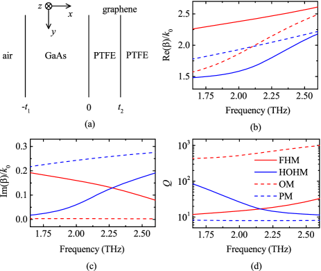
Figure 1: (Color Online) (a) Schematic of the hybrid graphene-based planar plasmonic waveguide, where $z$ is the propagation direction, $x$ is perpendicular to the interfaces, the thickness of GaAs is $t_{1}=20$ $\mu$m, the thickness of the left PTFE is $t_{2}=10$ $\mu$m, and the permittivities for air, GaAs, and PTFE are $\varepsilon_{1}=1$, $\varepsilon_{2}=13.06+0.01i$, and $\varepsilon_{3}=2.08+0.01i$, respectively. The parameters for the trilayer graphene are $\mu=$ 10 000 $\text{cm}^{2}/(\text{V}\cdot\text{s})$, $T=300$ K, and $\mu_{c}=0.3$ eV. (b)-(d) The real and imaginary parts of the propagation constants, and the quality factors of the hybrid modes versus frequency, respectively, where the solid red curves denote the fundamental hybrid mode (FHM) and the solid blue curves denote the higher order hybrid mode (HOHM). For comparison, the corresponding curves for the optical mode (OM) supported by air-GaAs-PTFE and plasmonic mode (PM) supported by PTFE-graphene-PTFE are also plotted in dashed red and blue, respectively.

Plasmonic waveguides based on nobel metals usually have low quality factors due to the strong Ohmic losses in metals. Even for graphene-based plasmonic waveguides, graphene plasmons also suffer from high dissipative loss Nanotechnology ; IEEEJSQE , although the surface conductivity of graphene is almost purely imaginary in the THz domain science332-1291 . In contrary, dielectric optical waveguides have high quality factors since the dielectric loss is low. If the optical mode in a dielectric optical waveguide and the plasmonic mode in a plasmonic waveguide are coupled, hybrid modes with moderate quality factors may exist.

Inspired by the hybrid plasmonic waveguides where both subwavelength confinement and long range propagation are fulfilled nphoton2-496 ; JLT32-3597 , and the flourishing developments of THz science and technology nmat1-26 , we propose a planar hybrid graphene-based plasmonic waveguide in the THz domain as an example. The structure is shown in Fig. 1(a), where $z$ is the propagation direction, $x$ is perpendicular to the interfaces, the thicknesses of GaAs and the left polytetrafluoroethylene (PTFE) are $t_{1}=20$ $\mu$m and $t_{2}=10$ $\mu$m, respectively. The thickness of the right PTFE can be treated as infinite as long as it is large enough compared with the skin depth of the waveguide mode. The permittivities for air, GaAs, and PTFE are $\varepsilon_{1}=1$, $\varepsilon_{2}=13.06+0.01i$ optical constants , and $\varepsilon_{3}=2.08+0.01i$ JKPS , respectively. GaAs and PTFE are widely used in THz waveguides and their permittivities are both assumed to be constants since their chromatic dispersions are small in the THz domain. The surface conductivity of trilayer graphene is $\sigma=3\sigma_{g}$ NL7-2711 ; nnano7-330 ; LPR8-291 , where $\sigma_{g}$ is the surface conductivity of monolayer graphene calculated by Kubo formula with $\mu=$ 10 000 $\text{cm}^{2}/(\text{V}\cdot\text{s})$, $T=300$ K, and $\mu_{c}=0.3$ eV JAP103-064302 ; JP19-026222 . Here, a trilayer graphene is used because it supports plasmonic modes with higher quality factors compared with those supported by the monolayer graphene APL101-111609 ; JLT32-3597 .

The hybrid modes supported by the hybrid plasmonic waveguide can be explained using the coupled mode theory (CMT). In CMT, the mode of an entire waveguide array is treated as a coupling between modes from single isolated waveguide channels waveguide theory . Following a similar procedure, the hybrid plasmonic waveguide shown in Fig. 1(a) can be divided into two isolated waveguide channels (a dielectric optical waveguide and a plasmonic waveguide) by increasing the thickness of middle PTFE to infinity, where the dielectric optical waveguide is composed by air-GaAs-PTFE, and the plasmonic waveguide is composed by PTFE-graphene-PTFE. Since the two channels are isolated from each other, the thicknesses of all PTFE layers in the two channels are infinite. For the dielectric optical waveguide, GaAs is used as a high refractive index material and a single TM optical mode (OM) is supported in the waveguide, where the dispersion relation and quality factor are shown by the dashed red lines in Fig. 1(b)-(c) and (d), respectively. Since the dielectric losses are low, the imaginary part of the propagation constant is small, and the optical mode has a high quality factor over the chosen frequency range. While for the plasmonic waveguide, PTFE is used both as the substrate and superstrate of the trilayer graphene and a TM plasmonic mode (PM) is supported, where the dispersion relation and quality factor are shown by the dashed blue lines. The plasmonic mode has a low quality factor due to the high Ohmic loss in graphene. For the hybrid plasmonic waveguide, the optical mode with a high quality factor and the plasmonic mode with a low quality factor can be coupled in phase and out of phase, leading to a fundamental mode and a higher order mode, respectively. As shown by the solid red lines, the fundamental hybrid mode (FHM) has the largest $\beta_{r}$ and the corresponding quality factor is high at higher frequencies with the decrease of $\beta_{i}$, while the higher order hybrid mode (HOHM) has the smallest $\beta_{r}$ and the corresponding quality factor is high at lower frequencies with the decrease of $\beta_{i}$, as shown by the solid blue lines.

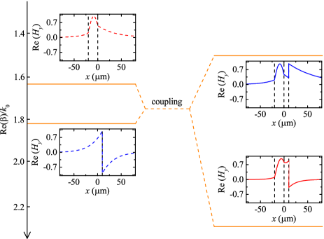
Figure 2: (Color Online) Propagation constants and corresponding field distributions of the modes before and after coupling at $f=1.75$ THz. The dashed black lines indicate the interfaces between different media, and the dashed yellow lines describe the coupling. The other parameters are $t_{1}=20$ $\mu$m, $t_{2}=10$ $\mu$m, $\varepsilon_{1}=1$, $\varepsilon_{2}=13.06+0.01i$, $\varepsilon_{3}=2.08+0.01i$, $\mu=$ 10 000 $\text{cm}^{2}/(\text{V}\cdot\text{s})$, $T=300$ K, and $\mu_{c}=0.3$ eV.

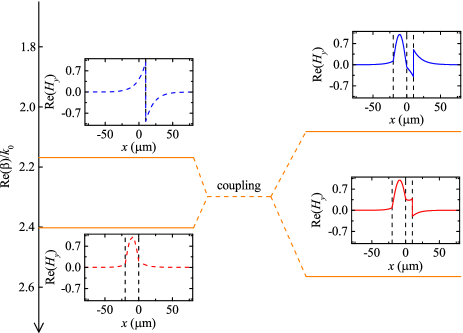
Figure 3: (Color Online) Propagation constants and corresponding field distributions of the modes before and after coupling at $f=2.50$ THz. The dashed black lines indicate the interfaces between different media, and the dashed yellow lines describe the coupling. The other parameters are the same as those shown in Fig. 2.

Fig. 2 shows the propagation constants and corresponding field distributions of the modes before and after coupling at $f=1.75$ THz. Before coupling, the plasmonic waveguide supports an anti-symmetric TM plasmonic mode with $\beta=1.82$, and the dielectric optical waveguide supports an asymmetric TM optical mode with $\beta=1.63$, where the quality factors are $Q=445.4$ and $Q=8.1$, respectively. At this frequency, the propagation constant of plasmonic mode is larger than that of the optical mode. After coupling, the fundamental mode has a quality factor of $Q=12.5$ with $\beta=2.30$, where the optical mode and the plasmonic mode are coupled in phase. While the higher order mode has a quality factor of $Q=61.4$ with $\beta=1.50$, where the optical mode and the plasmonic mode are coupled out of phase. This indicates that the higher order mode is little perturbed by the trilayer graphene compared with the fundamental mode, and it has a higher quality factor which is favourable for the implementation of Airy plasmons.

In contrast, Fig. 3 shows the propagation constants and corresponding field distributions of the modes before and after coupling at $f=2.50$ THz. Before coupling, the plasmonic mode has a quality factor of $Q=8.0$ with $\beta=2.17$, and the optical mode has a quality factor of $Q=907.2$ with $\beta=2.40$. At this frequency, the propagation constant of plasmonic mode is smaller than that of the optical mode. After coupling, the fundamental mode has a quality factor of $Q=26.8$ with $\beta=2.57$, and the higher order mode has a quality factor of $Q=12.0$ with $\beta=2.08$. In contrast to the hybrid modes at $f=1.75$ THz, the fundamental mode at $f=2.50$ THz has a higher quality factor compared with the higher order mode.

Clearly, the coupling between the optical mode and the plasmonic mode leads to the hybrid modes with moderate quality factors. For 1D Airy plasmons, if the waveguide mode distribution in $x$ direction is chosen as the hybrid mode with a higher quality factor, we can get a large enough transverse displacement under the fulfillment of Eq. (5).

II.3 Hybrid Airy plasmons

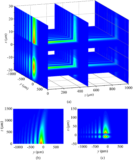
Figure 4: (Color Online) (a) The distributions of $\left|H_{y}\right|^{2}$ for hybrid Airy plasmons on two $y$-$z$ cut planes with $x=-t_{1}/2$ and $x=t_{2}$, and on three $x$-$y$ cut planes along the propagation direction with $z=0$ $\mu$m, $z=500$ $\mu$m, and $z=1000$ $\mu$m, respectively. The distributions at the $y$-$z$ plane with $x=t_{2}$ and the $x$-$y$ plane with $z=0$ are also shown in (b) and (c), respectively. The parameters for (a)-(c) are $a=0.1$, $f=1.75$ THz, $y_{0}=100$ $\mu$m, and $\mu_{c}=0.3$ eV.

For Airy plasmons in a hybrid plasmonic waveguide, if their transverse waveguide confinements are governed by the hybrid modes, these Airy plasmons can be called as hybrid Airy plasmons. In contrast to the Airy beams where the transverse waveguide confinements are governed by the optical modes JMO57-341 or plasmonic modes OL35-2082 , hybrid Airy plasmons are formed due to the coupling between an optical mode and a plasmonic mode.

Without loss of generality, we consider hybrid Airy plasmons where the transverse waveguide confinements are governed by the higher order hybrid mode at $f=1.75$ THz, since it has the highest quality factor within our parameter range. For simplicity, Fig. 4 shows the distributions of $\left|H_{y}\right|^{2}$ at different cut planes, where the scales of $x$, $y$, $z$ axis are different, and the parameters are $a=0.1$, $y_{0}=100$ $\mu$m, and $\mu_{c}=0.3$ eV. Note that Eq. (5) is valid under the above parameters. The distribution at the $y$-$z$ plane exhibits the diffraction-free and self-deflection behaviors of Airy plasmons, and the distribution at the $x$-$y$ plane is governed by the higher order hybrid mode in the hybrid plasmonic waveguide, where the width of the main lobe of hybrid Airy plasmons is much larger than its height. It is worth to note that, although the values of $\left|H_{y}\right|^{2}$ at two $y$-$z$ planes are nearly equal, the graphene-based plasmonic waveguide channel carries more energy if we use the standard definition of energy flux density $\left\langle S\right\rangle_{z}=\frac{1}{2}\text{Re}\left(E_{x}H_{y}^{\ast}\right)$.

As shown in Fig. 4(b), due to the high quality factor of the hybrid mode, the energy attenuation experienced by Airy plasmons is relatively small and the propagation length is comparably large, although the dissipative loss exists both in dielectric media and in trilayer graphene. Under the chosen parameters, the propagation length is $L_{n}=537.5$ $\mu$m ($L_{a}=558.9$ $\mu$m), and the corresponding transverse displacement at the propagation length is $\Delta y_{n}=24.0$ $\mu$m ($\Delta y_{a}=26.0$ $\mu$m), where the analytical results are nearly equal to the numerical results. The large transverse displacement is favourable for the detection and measurement of Airy plasmons experimentally. It is worth to note that, if the transverse waveguide confinement of Airy plasmons is governed by the plasmonic mode shown in Fig. 2 with $a=0.1$ and $y_{0}=100$ $\mu$m, the propagation length is $L_{n}=0.6$ $\mu$m ($L_{a}=0.6$ $\mu$m) and the corresponding transverse displacement at the propagation length is $\Delta y_{n}=1.0$ $\mu$m ($\Delta y_{a}=0.2$ $\mu$m). Our hybrid Airy plasmons show a better performance due to the moderate quality factor of the hybrid mode.

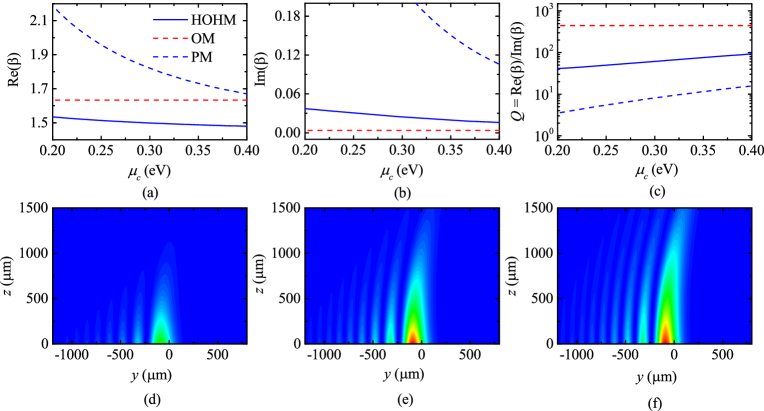
Figure 5: (Color Online) (a)-(c) The real and imaginary parts of the propagation constants, and the quality factors of the higher order hybrid mode (HOHM) versus the chemical potential of trilayer graphene, respectively. For comparison, the curves for the optical mode (OM) supported by air-GaAs-PTFE and plasmonic mode (PM) supported by PTFE-graphene-PTFE are also plotted in dashed red and blue, respectively, and the curves for the fundamental hybrid mode are omitted. (d)-(e) The distributions of $\left|H_{y}\right|^{2}$ at the $y$-$z$ plane with $x=t_{2}$ for $\mu_{c}=0.2$ eV, $\mu_{c}=0.3$ eV, and $\mu_{c}=0.4$ eV, respectively. The other parameters are $a=0.1$, $f=1.75$ THz, and $y_{0}=100$ $\mu$m.

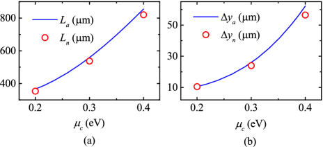
Figure 6: (Color Online) (a) Analytical propagation length $L_{a}$ and (b) transverse displacement $\Delta y_{a}$ of Airy plasmons versus the chemical potential of trilayer graphene. The numerical propagation length $L_{n}$ and transverse displacement $\Delta y_{n}$ for $\mu_{c}=0.2$ eV, $\mu_{c}=0.3$ eV, and $\mu_{c}=0.4$ eV are also plotted for comparison. The other parameters are $a=0.1$, $f=1.75$ THz, and $y_{0}=100$ $\mu$m.

For the effective trapping, transporting, and sorting of micro-objects, Airy plasmons with dynamically steerable trajectories are required. Since the self-deflection behavior is related with the propagation constant of the hybrid mode, we can tune the chemical potential of trilayer graphene dynamically by applying a gate voltage science332-1291 . As shown in Fig. 5 (a)-(c), for the higher order hybrid mode (HOHM), both the propagation constant and quality factor change effectively if the chemical potential is tuned from $0.2$ eV to $0.4$ eV (the curves for the fundamental hybrid mode are omitted), where the parameters are $a=0.1$, $f=1.75$ THz, and $y_{0}=100$ $\mu$m to insure the validity of Eq. (5). Clearly, when the chemical potential is large, the imaginary part of the propagation constant $\beta_{i}$ is small and the corresponding propagation length is large. The increases of the propagation length and quality factor lead to a larger transverse displacement of Airy plasmons, as shown by the distributions of $\left|H_{y}\right|^{2}$ at the $y$-$z$ plane with $x=t_{2}$ for $\mu_{c}=0.2$ eV, $\mu_{c}=0.3$ eV, and $\mu_{c}=0.4$ eV in Fig. 5 (a)-(c), respectively. Thus the transverse displacement is dynamically steerable by changing the chemical potential of graphene (See Supporting Information).

To quantitatively show the steerable trajectories by tuning the chemical potential of trilayer graphene, we plot the numerical propagation lengths $L_{n}$ and transverse displacements $\Delta y_{n}$ for $\mu_{c}=0.2$ eV, $\mu_{c}=0.3$ eV, and $\mu_{c}=0.4$ eV as well as the analytical counterparts in Fig. 6. The consistency between the analytical and numerical results not only confirms the validity of the paraxial approximation which insures the non-diffracting behavior of Airy plasmons, but also demonstrates the feasibility of dynamically steerable trajectories of hybrid Airy plasmons.

Finally, we would like to note that, our hybrid Airy plasmons can be realized experimentally by considering both the waveguide fabrication and Airy plasmons excitation. For the waveguide fabrication, all the materials including GaAs, PTFE, and graphene are widely used in THz waveguides. Graphene can be grown well by a CVD reaction between CH${}_{\text{4}}$ and H${}_{\text{2}}$ on copper substrate, which can be etched away using acid solution. The suspended graphene can subsequently be transferred to arbitrary substrate. Recently, we have designed a graphene/GaAs van der Waals heterostructure solar cell NE16-310 and studied the electric power generation from a single moving droplet on graphene/PTFE ACSNano10-7297 . The wet transfer technique that used in the two experiments can be directly applied to fabricate the hybrid graphene-based plasmonic waveguide. While for the Airy plasmons excitation, it includes two steps: the generation of surface plasmon polaritons (SPPs) and the generation of Airy plasmons. The two steps can be accomplished simultaneously by a delicately designed grating PRL107-116802 ; OL38-1443 . Alternatively, a laser beam can be coupled into SPPs by grating, and Airy plasmons can be generated by a nonperiodically arranged nanocave array PRL107-126804 .

III Conclusion

In conclusion, we reveal the hybrid Airy plasmons for the first time by taking a hybrid graphene-based plasmonic waveguide in the THz domain as an example. Due to the moderate quality factors of the hybrid modes, hybrid Airy plasmons where the transverse waveguide confinements are governed by the hybrid modes can have large propagation lengths and effective transverse deflections, and they are promising to solve the long standing problems for the experimental observation and implementation of Airy plasmons. Meanwhile, the propagation trajectories of hybrid Airy plasmons are dynamically steerable by changing the chemical potential of trilayer graphene. This interesting finding may lead to the flexible optical micromanipulation in flatland plasmonic devices and chip scale signal processing, and the hybrid Airy plasmons may promote the further discovery of non-diffracting beams with the emerging developments of optical tweezers and tractor beams.

IV Methods

IV.1 Paraxial Wave Equation

Airy beams propagating in a planar waveguide can be described by the 1D paraxial wave equation which is similar with the Schrödinger equation in quantum mechanics. For simplicity, we assume that Airy beams are perturbations of the waveguide modes, and they behave as quasi-TM or quasi-TE modes approximately. The Helmholtz equation is

$$\nabla^{2}\Phi+k_{0}^{2}\varepsilon\left(x\right)\Phi=0,$$ (8)

where $\varepsilon\left(x\right)$ is the distribution of relative permittivity, $\Phi=H_{y}(x,y,z)$ for the quasi-TM Airy beams, and $\Phi=E_{y}(x,y,z)$ for the quasi-TE Airy beams. The scalar field $\Phi\left(x,y,z\right)$ can be expressed as a functional dependence of the form JMO57-341

$$\Phi\left(x,y,z\right)=\psi\left(y,z\right)\Phi_{0}\left(x\right)\exp\left(i\beta z\right),$$ (9)

where the dimensionless scalar function $\psi\left(y,z\right)$ is dependent on both the transverse direction $y$ and the propagation direction $z$, the scalar function $\Phi_{0}\left(x\right)$ is only dependent on the transverse direction $x$, and $\beta$ is a parameter that is related to the $z$ component of the wavevector. Substituting Eq. (9) into Eq. (8), multiplying the result by $\Phi_{0}^{\ast}\left(x\right)$, and integrating over $x$ direction yields a scalar wave equation

$$\left[2i\beta\frac{\partial\psi}{\partial z}+\frac{\partial^{2}\psi}{\partial y^{2}}\right]+\left[\frac{I_{2}}{I_{0}}+k_{0}^{2}\varepsilon\left(x\right)-\beta^{2}\right]\psi=0,$$ (10)

where $I_{0}=\int_{-\infty}^{+\infty}\left|\Phi_{0}\left(x\right)\right|^{2}dx$, $I_{2}=\int_{-\infty}^{+\infty}\Phi_{0}^{\prime\prime}\left(x\right)\Phi_{0}^{\ast}\left(x\right)dx$, and the term $\partial^{2}\psi/\partial z^{2}$ is neglected by employing the paraxial approximation OL35-2082 ; OL32-674 . Note the functional dependence between $\psi$ and $x$ is neglected for step index waveguides or graded index waveguides with $\nabla\varepsilon\approx 0$. For the slowly varying amplitude, the scalar function is expressed as $\psi\left(y,z\right)=\phi\left(y,z\right)\exp\left\{i\left[I_{2}/I_{0}+k_{0}^{2}\varepsilon\left(x\right)-\beta^{2}\right]/\left(2\beta\right)z\right\}$, which leads to the one-dimensional paraxial wave equation $i\phi_{z}\left(y,z\right)+\left(1/2\beta\right)\phi_{yy}\left(x,z\right)=0$. If the function $\Phi_{0}\left(x\right)$ is chosen as the magnetic (electric) field distribution of TM (TE) waveguide mode, and the parameter $\beta=\beta_{r}+i\beta_{i}$ is the corresponding propagation constant, $I_{2}/I_{0}+k_{0}^{2}\varepsilon\left(x\right)-\beta^{2}=0$ and the paraxial wave equation for the amplitude $\psi$ is

$$i\frac{\partial\psi\left(s,\xi\right)}{\partial\xi}+\frac{\partial^{2}\psi\left(s,\xi\right)}{\partial s^{2}}=0,$$ (11)

where $s=y/y_{0}$ is the dimensionless transverse coordinate, $\xi=z/2\beta y_{0}^{2}$ is the dimensionless complex propagation distance, and $y_{0}$ is an arbitrary transverse scale.

IV.2 Dispersion relation for hybrid modes

Dispersion relation for hybrid modes in the hybrid graphene-based planar plasmonic waveguide can be calculated by standard waveguide theory waveguide theory , where the field components in each region are derived from Helmholtz equation, and the propagation constant is determined by imposing appropriate boundary conditions. For the structure shown in Fig. 1, the magnetic field distribution can be written as follows

$$H_{y}\left(x\right)=\left\{\begin{array}[c]{ll}Ae^{k_{1}x}e^{i\beta z},&x\leq-t_{1},\\ B\sin\left(k_{2}x\right)e^{i\beta z}+C\cos\left(k_{2}x\right)e^{i\beta z},&-t_{1}<x\leq 0,\\ De^{k_{3}x}e^{i\beta z}+Ee^{-k_{3}x}e^{i\beta z},&0<x\leq t_{2},\\ Fe^{-k_{3}x}e^{i\beta z},&x>t_{2},\end{array}\right.$$ (12)

where $k_{1}=\sqrt{\beta^{2}-k_{0}^{2}\varepsilon_{1}}$, $k_{2}=\sqrt{k_{0}^{2}\varepsilon_{2}-\beta^{2}}$, $k_{3}=\sqrt{\beta^{2}-k_{0}^{2}\varepsilon_{3}}$, $k_{0}=2\pi f/c$ is the wavenumber in free space, $f$ is the frequency, and $\varepsilon_{1}$, $\varepsilon_{2}$, and $\varepsilon_{3}$ are relative permittivities of air, GaAs, and PTFE, respectively. Considering the boundary conditions, the dispersion relation is

$$e^{-2k_{3}t_{2}}=\frac{\alpha_{+}\left[\beta_{-}\tan\left(k_{2}t_{1}\right)+\gamma_{+}\right]}{\alpha_{-}\left[\beta_{+}\tan\left(k_{2}t_{1}\right)-\gamma_{-}\right]},$$ (13)

where $\alpha_{\pm}=\left(1+i\sigma k_{3}/\omega\varepsilon_{0}\varepsilon_{3}\right)\left(k_{3}/\varepsilon_{3}\right)\pm\left(k_{3}/\varepsilon_{3}\right)$, $\beta_{\pm}=\left(k_{1}/\varepsilon_{1}\right)\left(k_{3}/\varepsilon_{3}\right)\pm\left(k_{2}/\varepsilon_{2}\right)^{2}$, $\gamma_{\pm}=\left(k_{2}/\varepsilon_{2}\right)\left[\left(k_{1}/\varepsilon_{1}\right)\pm\left(k_{3}/\varepsilon_{3}\right)\right]$, and $\sigma$ is the surface conductivity of trilayer graphene.

The hybrid modes are formed by the coupling between the optical modes in dielectric waveguide and the plasmonic modes in graphene-based plasmonic waveguide. The dispersion relation for the optical modes in dielectric waveguide is

$$\tan\left(k_{2}t_{1}\right)=-\frac{\gamma_{+}}{\beta_{-}},$$ (14)

which can be obtained by setting $\sigma=0$ in Eq. (13). While for the plasmonic modes in graphene-based plasmonic waveguide science332-1291 , the dispersion relation is

$$\beta=k_{0}\sqrt{\varepsilon_{3}-\left(\frac{2\varepsilon_{3}}{\sigma\eta_{0}}\right)^{2}},$$ (15)

where $\eta_{0}=\sqrt{\mu_{0}/\varepsilon_{0}}$ is the wave impendence in free space.

The surface conductivity of monolayer graphene can be calculated by Kubo formula $\sigma_{g}\left(\omega,\mu_{c},\Gamma,T\right)=\sigma_{\text{intra}}+\sigma_{\text{inter}}$, where

$$\sigma_{\text{intra}}=\frac{ie^{2}k_{B}T}{\pi\hbar^{2}\left(\omega+i\tau^{-1}\right)}\left[\frac{\mu_{c}}{k_{B}T}+2\ln\left(e^{-\mu_{c}/k_{B}T}+1\right)\right]$$ (16)

is due to intraband contribution,

$$\sigma_{\text{inter}}=\frac{ie^{2}\left(\omega+i\tau^{-1}\right)}{\pi\hbar^{2}}\int_{0}^{\infty}\frac{f_{d}\left(-\varepsilon\right)-f_{d}\left(\varepsilon\right)}{\left(\omega+i\tau^{-1}\right)^{2}-4\left(\varepsilon/\hbar\right)^{2}}d\varepsilon$$ (17)

is due to interband contribution JAP103-064302 ; JP19-026222 , and the nonlocal effects are neglected PRB80-245435 . In the above formula, $-e$ is the charge of an electron, $\hbar=h/2\pi$ is the reduced Plank’s constant, $T$ is the temperature, $\mu_{c}$ is the chemical potential, $\tau=\mu\mu_{c}/ev_{F}^{2}$ is the carrier relaxation time, $\mu$ is the carrier mobility which ranges from 1 000 $\text{cm}^{2}/(\text{V}\cdot\text{s})$ to 230 000 $\text{cm}^{2}/(\text{V}\cdot\text{s})$ ACSnano , $v_{F}=c/300$ is the Fermi velocity, $f_{d}\left(\varepsilon\right)=1/\left[e^{\left(\varepsilon-\mu_{c}\right)/k_{B}T}+1\right]$ is the Fermi-Dirac distribution, and $k_{B}$ is the Boltzmann’s constant. In this paper, we use a moderate mobility of $\mu=$ 10 000 $\text{cm}^{2}/(\text{V}\cdot\text{s})$, $T=300$ K, and the chemical potential $\mu_{c}$ is tuned from $0.2$ eV to $0.4$ eV.

V acknowledgement

We are grateful to Mr. Huikai Zhong for his valuable discussion. This work was sponsored by the National Natural Science Foundation of China under Grants No. 61322501, No. 61574127, and No. 61275183, the Top-Notch Young Talents Program of China, the Program for New Century Excellent Talents (NCET-12-0489) in University, the Fundamental Research Funds for the Central Universities, and the Innovation Joint Research Center for Cyber-Physical-Society System. X. Lin acknowledges the support from Chinese Scholarship Council (CSC No. 201506320075).

References

- (1) M. V. Berry and N. L. Balazs, Nonspreading wave packets, Am. J. Phys. 47, 264 (1979)
- (2) G. A. Siviloglou and D. N. Christodoulides, Accelerating finite energy Airy beams, Opt. Lett. 32, 979 (2007).
- (3) M. Mazilu, D. J. Stevenson, F. G.-Moore, and K. Dholakia, Light beats the spread: “non-diffracting” beams, Laser Photonics Rev. 4, 529 (2010).
- (4) I. M. Besieris and A. M. Shaarawi, A note on an accelerating finite energy Airy beam, Opt. Lett. 32, 2447 (2007).
- (5) G. A. Siviloglou, J. Broky, A. Dogariu, and D. N. Christodoulides, Observation of accelerating Airy beams, Phys. Rev. Lett. 99, 213901 (2007).
- (6) J. Broky, G. A. Siviloglou, A. Dogariu, and D. N. Christodoulides, Self-healing properties of optical Airy beams, Opt. Exp. 16, 12880 (2008).
- (7) N. K. Efremidis and D. N. Christodoulides, Abruptly autofocusing waves, Opt. Lett. 35, 4045 (2010).
- (8) D. G. Papazoglou, N. K. Efremidis, D. N. Christodoulides, and S. Tzortzakis, Observation of abruptly autofocusing waves, Opt. Lett. 36, 1842 (2011).
- (9) J. Baumgartl, M. Mazilu, and K. Dholakia, Optically mediated particle clearing using Airy wavepackets, Nat. Photon. 2, 675 (2008).
- (10) P. Zhang, J. Prakash, Z. Zhang, M. S. Mills, N. K. Efremidis, D. N. Christodoulides, and Z. Chen, Trapping and guiding microparticles with morphing autofocusing Airy beams, Opt. Lett. 36, 2883 (2011).
- (11) Z. Zheng, B.-F. Zhang, H. Chen, J. Ding, and H.-T. Wang, Optical trapping with focused Airy beams, Appl. Opt. 50, 43 (2011).
- (12) Y. Liang, Y. Hu, D. Song, C. Lou, X. Zhang, Z. Chen, and J. Xu, Image signal transmission with Airy beams, Opt. Lett. 40, 5686 (2015).
- (13) P. Rose, F. Diebel, M. Boguslawski, and C. Denz, Airy beam induced optical routing, Appl. Phys. Lett. 102, 101101 (2013).
- (14) N. Wiersma, N. Marsal, M. Sciamanna, and D. Wolfersberger, All-optical interconnects using Airy beams, Opt. Lett. 39, 5997 (2014).
- (15) A. Chong, W. H. Renninger, D. N. Christodoulides, and F. W. Wise, Airy-Bessel wave packets as versatile linear light bullets, Nat. Photon. 4, 103 (2010).
- (16) P. Saari, Laterally accelerating Airy pulses, Opt. Exp. 16, 10303 (2008).
- (17) K.-Y. Kim, C.-Y. Hwang, and B. Lee, Slow non-dispersing wavepackets, Opt. Exp. 19, 2286 (2011).
- (18) T. Schneider, A. A. Serga, A. V. Chumak, C. W. Sandweg, S. Trudel, S. Wolff, M. P. Kostylev, V. S. Tiberkevich, A. N. Slavin, and B. Hillebrands, Nondiffractive subwavelength wave beams in a medium with externally controlled anisotropy, Phys. Rev. Lett. 104, 197203 (2010).
- (19) S. Fu, Y. Tsur, J. Zhou, L. Shemer, and A. Arie, Propagation Dynamics of Airy Water-Wave Pulses, Phys. Rev. Lett. 115, 034501 (2015).
- (20) N. V.-Bloch, Y. Lereah, Y. Lilach, A. Gover, and A. Arie, Generation of electron Airy beams, Nature 494, 331 (2013).
- (21) N. K. Efremidis, and V. Paltoglou, Accelerating and abruptly autofocusing matter waves, Phys. Rev. A 87, 043637 (2013).
- (22) A. Salandrino, and D. N. Christodoulides, Airy plasmon: a nondiffracting surface wave, Opt. Lett. 35, 2082 (2010).
- (23) Y. Yang, H. T. Dai, B. F. Zhu, and X. W. Sun, Dynamic Control of the Airy Plasmons in a Graphene Platform, IEEE Photonics J. 6, 4801207 (2014).
- (24) A. Minovich, A. E. Klein, N. Janunts, T. Pertsch, D. N. Neshev, and Y. S. Kivshar, Generation and Near-Field Imaging of Airy Surface Plasmons, Phys. Rev. Lett. 107, 116802 (2011).
- (25) L. Li, T. Li, S. M. Wang, C. Zhang, and S. N. Zhu, Plasmonic Airy Beam Generated by In-Plane Diffraction, Phys. Rev. Lett. 107, 126804 (2011).
- (26) A. V. Novitsky, and D. V. Novitsky, Nonparaxial Airy beams: role of evanescent waves, Opt. Lett. 34, 3430 (2009).
- (27) P. Zhang, S. Wang, Y. Liu, X. Yin, C. Lu, Z. Chen, and X. Zhang, Plasmonic Airy beams with dynamically controlled trajectories, Opt. Lett. 36, 3191 (2011).
- (28) W. Liu, D. N. Neshev, I. V. Shadrivov, A. E. Miroshnichenko, and Y. S. Kivshar, Plasmonic Airy beam manipulation in linear optical potentials, Opt. Lett. 36, 1164 (2011).
- (29) F. Bleckmann, A. Minovich, J. Frohnhaus, D. N. Neshev, and S. Linden, Manipulation of Airy surface plasmon beams, Opt. Lett. 38, 1443 (2013).
- (30) A. E. Minovich, A. E. Klein, D. N. Neshev, T. Pertsch, Y. S. Kivshar, and D. N. Christodoulides, Airy plasmons: non-diffracting optical surface waves, Laser Photon. Rev. 8, 221 (2014).
- (31) R. F. Oulton, V. J. Sorger, D. A. Genov, D. F. P. Pile, and X. Zhang, A hybrid plasmonic waveguide for subwavelength confinement and long range propagation, Nat. Photon. 2, 496 (2008).
- (32) X. Zhou, T. Zhang, L. Chen, W. Hong, and X. Li, A Graphene-Based Hybrid Plasmonic Waveguide With Ultra-Deep Subwavelength Confinement, J. Lighwave Techno. 32, 3597 (2014).
- (33) M. Abramowitz, and I. A. Stegun, Handbook of Mathematical Functions (Dover, 1972).
- (34) A. R. Davoyan and N. Engheta, Salient Features of Deeply Subwavelength Guiding of Terahertz Radiation in Graphene-Coated Fibers, ACS Photonics 3, 737 (2016).
- (35) R. Li, X. Lin, S. Lin, X. Liu, and Hongsheng Chen, Atomically thin spherical shell-shaped superscatterers based on a Bohr model, Nanotechnology 26, 505201 (2015).
- (36) R. Li, B. Zheng, X. Lin, R. Hao, S. Lin, W. Yin, E. Li, and H. Chen, Design of Ultracompact Graphene-Based Superscatterers, IEEE J. Sel. Top. Quant. 23, 4600208 (2017).
- (37) A. Vakil, and N. Engheta, Transformation Optics Using Graphene, Science 332, 1291 (2011).
- (38) B. Ferguson and X.-C. Zhang, Materials for terahertz science and technology, Nat. Mat. 1, 26 (2002).
- (39) D. Palik, Handbook of Optical Constants of Solids (Academic Press, 1998).
- (40) Y.-S. Jin, G.-J. Kim, and S.-G. Jeon, Terahertz Dielectric Properties of Polymers, J. Korean Phys. Soc. 49, 513 (2006).
- (41) C. Casiraghi, A. Hartschuh, E. Lidorikis, H. Qian, H. Harutyunyan, T. Gokus, K. S. Novoselov, and A. C. Ferrari, Rayleigh Imaging of Graphene and Graphene Layers, Nano Lett. 7, 2711 (2007).
- (42) H. Yan, X. Li, B. Chandra, G. Tulevski, Y. Wu, M. Freitag, W. Zhu, P. Avouris, and F. Xia, Tunable infrared plasmonic devices using graphene/insulator stacks, Nat, Nanotech. 7, 330 (2012).
- (43) D. A. Smirnova, I. V. Shadrivov, A. I. Smirnov, and Y. S. Kivshar, Dissipative plasmon-solitons in multilayer graphene, Laser Photonics Rev. 8, 291 (2014).
- (44) G. W. Hanson, Dyadic Green’s functions and guided surface waves for a surface conductivity model of graphene, J. Appl. Phys. 103, 064302 (2008).
- (45) V. P. Gusynin, S. G. Sharapov, and J. P. Carbotte, Magneto-optical conductivity in graphene, J. Phys. 19, 026222 (2007).
- (46) C. H. Gan, Analysis of surface plasmon excitation at terahertz frequencies with highly doped graphene sheets via attenuated total reflection, Appl. Phys. Lett. 101, 111609 (2012).
- (47) K. Okamoto, Fundamentals of Optical Waveguides (Elsevier, 2006).
- (48) V. Lakshminarayanana, and K. Thyagarajan, Non-diffracting Airy beams in planar optical waveguides: a convenient method for visualization, J. Mod. Opt. 57, 341 (2010).
- (49) X. Li, W. Chen, S. Zhang, Z. Wu, P. Wang, Z. Xu, H. Chen, W. Yin, H. Zhong, S. Lin, 18.5% efficient graphene/GaAs van der Waals heterostructure solar cell, Nano Energy 16, 310 (2015).
- (50) S. S. Kwak, S. Lin, J. H. Lee, H. Ryu, T. Y. Kim, H. Zhong, H. Chen, and S.-W. Kim, Triboelectrification-Induced Large Electric Power Generation from a Single Moving Droplet on Graphene/Polytetrafluoroethylene, ACS Nano 10, 7297 (2016).
- (51) E. Feigenbaum, and M. Orenstein, Plasmon-soliton, Opt. Lett. 32, 674 (2007).
- (52) M. Jablan, H. Buljan, and M. Soljačić, Plasmonics in graphene at infrared frequencies, Phys. Rev. B 80, 245435 (2009).
- (53) W. Gao, J. Shu, C. Qiu, and Q. Xu, Excitation of Plasmonic Waves in Graphene by Guided-Mode Resonances, ACS Nano 6, 7806 (2012).