In-medium dispersion relations of charmonia studied by maximum entropy method

Abstract

We study in-medium spectral properties of charmonia in the vector and pseudoscalar channels at nonzero momenta on quenched lattices, especially focusing on their dispersion relation and weight of the peak. We measure the lattice Euclidean correlation functions with nonzero momenta on the anisotropic quenched lattices and study the spectral functions with the maximum entropy method. The dispersion relations of charmonia and the momentum dependence of the weight of the peak are analyzed with the maximum entropy method together with the errors estimated probabilistically in this method. We find significant increase of the masses of charmonia in medium. It is also found that the functional form of the charmonium dispersion relations is not changed from that in the vacuum within the error even at $T\simeq 1.6T_{\rm c}$ for all the channels we analyzed.

I introduction

Understanding properties of heavy quarkonia in hot medium near and above the critical temperature $T_{\rm c}$ of the deconfinement phase transition is one of the important subjects in relativistic heavy ion collisions Brambilla et al. (2011); Andronic et al. (2016). It is believed that, by understanding the stabilities of heavy quarkonia, their yields in heavy ion collisions can be used as a signal of the formation of the quark-gluon plasma Matsui and Satz (1986). Because of their heavy mass, heavy quarks (charm and bottom quarks and their antiparticles) also serve as unique theoretical and experimental probes to diagnose the properties of the hot medium, such as the heavy-quark potential Hashimoto et al. (1986) and the transport properties Akamatsu et al. (2009). Experimental progress in this field, such as the isolation of charm and bottom quarks using the silicon vertex tracker PHENIX Collaboration et al. (2009), will enrich the study of heavy quarks further.

The hot matter created by heavy ion collisions with temperature ($T$) near $T_{\rm c}$ is believed to be a strongly interacting system. Lattice QCD is a powerful method to investigate such a region of QCD at which nonperturbative effects will play a crucial role. The study of the properties of charmonia at finite temperature is one of the longstanding subjects on the lattice Asakawa and Hatsuda (2004); Datta et al. (2004a); Umeda et al. (2004); Datta et al. (2005); Jakovác et al. (2007); Umeda (2007); WHOT-QCD Collaboration et al. (2011); Ding et al. (2012); Borsányi et al. (2014). In lattice QCD numerical simulations, which rely on the imaginary time formalism, however, one cannot analyze dynamical properties encoded in spectral functions directly. Instead, only Euclidean correlation functions are calculable on the lattice. To obtain the spectral functions from the Euclidean correlators, one has to take an analytic continuation from imaginary time to real time. The maximum entropy method (MEM) is a useful method to perform this analytic continuation on the basis of probability theory. Jarrell and Gubernatis (1996); Asakawa et al. (2001). The studies of charmonium spectral functions with MEM qualitatively agree with each other in that the charmonia in the vector and pseudoscalar channels survive up to around $T\simeq 1.5T_{\rm c}$ Asakawa and Hatsuda (2004); Datta et al. (2004a, 2005); Borsányi et al. (2014).

In the previous studies on heavy quarkonia on the lattice, the analyses have been performed only for zero momentum with a few exceptions Datta et al. (2004b); Nonaka et al. (2011); Oktay and Skullerud (2010); Aarts et al. (2013); Ding (2013). The spectral function with zero momentum represents the spectral properties of a charmonium at rest in medium. On the other hand, charmonia in the hot medium created by heavy ion collisions typically have nonnegligible velocity against the rest frame of the medium because charmonia generated by hard processes in the early stage can have large momentum. The finiteness of the velocity of charmonia may modify their properties, such as the stability Liu et al. (2007) and the dispersion relation, i.e. the momentum dependence of energy. Here it is worthwhile to note that such modifications of the dispersion relations in medium are suggested in various systems Bellac (2000); Shuryak (1990); Pisarski and Tytgat (1996), and such a modification can give rise to novel phenomena such as van Hove singularity Van Hove (1953); Braaten et al. (1990); Kitazawa et al. (2014); Kim et al. (2015). It thus is interesting to explore the momentum dependence of spectral functions of charmonia and their dispersion relations near and above $T_{\rm c}$ with the first principle simulation on the lattice. The purpose of the present study is to perform a quantitative study on the momentum dependence of charmonium spectral functions on the lattice with MEM.

In this study we explore the properties of charmonia in the vector and pseudoscalar channels, corresponding to $J/\psi$ and $\eta_{c}$, respectively, at nonzero momenta on anisotropic quenched lattices. In addition to the standard analysis of the spectral functions in MEM, we study the dispersion relations and the momentum dependence of the spectral weights of the $J/\psi$ and $\eta_{c}$ peaks on the basis of MEM. To perform the measurement of the dispersion relation with a quantitative error analysis in MEM, we analyze the center of weight of the peak in the spectral function. As we will see later, this quantity is identical to the peak position for sufficiently narrow peaks, but error analysis can be carried out in MEM. Similarly, we analyze the weight of the peak, which corresponds to the residue of the peak, with the error analysis. For the vector channel, the transverse and longitudinal components are investigated separately in the analysis.

We find that the masses of $J/\psi$ and $\eta_{c}$ defined by the dispersion relation at zero momentum show significant increase as $T$ is raised. It is also found that the dispersion relation of charmonia continues to take the Lorentz covariant form, i.e. the same form as in the vacuum, even well above $T_{\rm c}$ within the error. Our numerical analysis also suggests that the weight of the peak at finite temperature does not have momentum dependence within the error.

This paper is organized as follows. In Sec. II, we introduce the spectral function and summarize its properties. We then discuss MEM in Sec. III. The error estimate in this method and the quantities corresponding to the dispersion relation and spectral weight of charmonia are discussed in this section. In Sec. IV, we show our lattice set up. We then discuss the numerical results in Sec. V. Sec. VI is devoted to conclusion.

II Euclidean correlator and spectral function

Dynamical properties of charmonia are encoded in the Euclidean correlators

$$G^{lm}(\tau,\vec{p})=\int d^{3}xe^{i\vec{p}\cdot\vec{x}}\left\langle J^{l}(\tau,\vec{x})J^{m\dagger}(0,\vec{0})\right\rangle,$$ (1)

where the imaginary time $\tau$ is restricted to the interval $0\leq\tau<1/T$ and $J^{l}(\tau,\vec{x})=\bar{c}(\tau,\vec{x})i\gamma^{l}c(\tau,\vec{x})$ is the local interpolating operator in the Heisenberg representation with the charm quark field $c(\tau,\vec{x})$ with $l=0,1,2,$ and $3$ for the vector channel and $l=5$ for the pseudoscalar channel. The spectral function $A^{lm}(\omega,\vec{p})$ is defined as the imaginary part of the retarded correlator $G^{lm}_{\rm R}(\omega,\vec{p})$ divided by $\pi$,

$$A^{lm}(\omega,\vec{p}) =\frac{1}{\pi}{\rm Im}\left[G^{lm}_{\rm R}(\omega,\vec{p})\right],$$ (2)

where

$$G^{lm}_{\rm R}(\omega,\vec{p}) =\int_{-\infty}^{\infty}dt\int d^{3}\vec{x}e^{-i\vec{p}\cdot\vec{x}+i\omega t}G^{lm}_{\rm R}(t,\vec{x}),$$ (3)

$$G^{lm}_{\rm R}(t,\vec{x}) =i\theta(t)\langle[J^{l}(t,\vec{x}),J^{m\dagger}(0,\vec{0})]\rangle.$$ (4)

The diagonal components of the spectral functions $A^{ll}(\omega,\vec{p})$ are related to Eq. (1) by the Laplace-like transformation as

$$G^{ll}(\tau,\vec{p})=\int_{0}^{\infty}{K}(\tau,\omega){A^{ll}}{(\omega,\vec{p})}d\omega,$$ (5)

with

$$K(\tau,\omega)=\frac{e^{-\tau\omega}+e^{-(1/T-\tau)\omega}}{1-e^{-\omega/T}}.$$ (6)

In the following, we represent the diagonal components of the spectral functions as

$$A^{l}(\omega,\vec{p})=A^{ll}(\omega,\vec{p}).$$ (7)

In the vacuum, as a consequence of Lorentz invariance and charge conservation, the vector spectral function can be represented as

$$A^{\mu\nu}(\omega,\vec{p})=\left(\frac{p^{\mu}p^{\nu}}{P^{2}}-g^{\mu\nu}\right)A_{\rm V}(P^{2}),$$ (8)

with $\mu,\nu=0,1,2,$ and $3$ and $P^{2}=\omega^{2}-|\vec{p}|^{2}$. When there is a bound state which couples to $J^{l}$, the corresponding spectral function $A_{\rm V}(\omega,p)=A_{\rm V}(P^{2})$ or $A_{\rm PS}(\omega,p)=A^{5}(\omega,\vec{p})$ has a peak structure around $\omega\simeq\pm E({p})$, where $E({p})$ is the dispersion relation of the bound state with $p=|\vec{p}|$. The peak structure is approximately be given by a delta function,

$$Z\delta(\omega^{2}-E(p)^{2})=\frac{Z}{2E(p)}\delta\left(\omega-E(p)\right),$$ (9)

where the right hand side represents the peak at $\omega>0$, and $Z>0$ is the residue. Because of Lorentz invariance, $E(p)$ in the vacuum is given by

$$E(p)=\sqrt{m^{2}+p^{2}},$$ (10)

where $m$ is the mass of the bound state. It is also shown from Lorentz invariance that $Z$ in Eq. (9) does not have momentum dependence.

The property of the bound state peak in Eqs. (9) and (10) is modified at finite temperature. First, the width of the peak becomes larger and the delta function in Eq. (9) is replaced by a smooth function with a peak. Second, because Lorentz invariance is lost in medium, $Z$ can depend on momentum. The dispersion relation $E(p)$ can also be modified from the Lorentz covariant form Eq. (10).

At finite temperature, $A^{\mu\nu}(\omega,\vec{p})$ in Eq. (8) is decomposed into the transverse and longitudinal components as Kapusta and Gale (2006)

$$A^{\mu\nu}(\omega,\vec{p})=P_{\rm T}^{\mu\nu}A_{\rm T}(\omega,p)+P_{\rm L}^{\mu\nu}A_{\rm L}(\omega,p),$$ (11)

where the projection operators onto the transverse and longitudinal components, $P_{\rm T}$ and $P_{\rm L}$, respectively, are defined as

$$P_{\rm T}^{00}=P_{\rm T}^{0i}=P_{\rm T}^{i0}=0,$$ (12)

$$P_{\rm T}^{ij}=\delta^{ij}-p^{i}p^{j}/p^{2},$$ (13)

$$P_{\rm L}^{\mu\nu}=p^{\mu}p^{\nu}/P^{2}-g^{\mu\nu}-P_{\rm T}^{\mu\nu},$$ (14)

with $i,j=1,2,$ and $3$. The transverse and longitudinal spectral functions $A_{\rm T}(\omega,p)$ and $A_{\rm L}(\omega,p)$ are identical in the vacuum, $A_{\rm T}(\omega,p)=A_{\rm L}(\omega,p)=A_{\rm V}(\omega,p)$, from Eq. (8). When the momentum is taken as $\vec{p}=(p,0,0)$, $A_{\rm T}(\omega,p)$ and $A_{\rm L}(\omega,p)$ are related to $A^{i}(\omega,\vec{p})$ as

$$A_{\rm T}(\omega,p) =\frac{1}{2}\left(A^{2}(\omega,\vec{p})+A^{3}(\omega,\vec{p})\right),$$ (15)

$$A_{\rm L}(\omega,p) =\frac{\omega^{2}-{p}^{2}}{\omega^{2}}A^{1}(\omega,\vec{p}).$$ (16)

From the general property of the spectral function, $A^{l}(\omega,\vec{p})$ are semi-positive for $\omega>0$ Kapusta and Gale (2006). The semi-positivity of $A_{\rm T}(\omega,p)$ is then guaranteed from Eq. (15). On the other hand, Eq. (16) shows that $A_{\rm L}(\omega,p)$ is semi-negative in the space-like region $0<\omega<p$.

III maximum entropy method

In this section we give a briefly review of MEM and show how the dispersion relations and spectral weights of charmonia are estimated in our analysis using MEM.

To obtain the spectral function from the lattice Euclidean correlator, we have to take the inverse transformation of Eq. (5). MEM Jarrell and Gubernatis (1996); Asakawa et al. (2001) is a method to infer the most probable image of the spectral function from a limited number of data points for a Euclidean correlator on the basis of Bayes’ theorem.

In the analysis of a spectral function $A(\omega)$ corresponding to a Euclidean correlator $G(\tau)$ obtained in a Monte Carlo simulation with Eq. (5), the most important quantity is the $\chi$-square,

$$\chi^{2}=\sum_{i,j}\left(G(\tau_{i})-G_{A}(\tau_{i})\right)C_{ij}^{-1}\left(G(\tau_{j})-G_{A}(\tau_{j})\right),$$ (17)

where the correlation between different temporal points $\tau_{i}$ is encoded in the covariance matrix $C_{ij}$, $i$ and $j$ run over discrete temporal points and $G_{A}(\tau_{i})$ is the correlator defined by Eq. (5) from the spectral function $A(\omega)$.

In the standard least-square method, $A(\omega)$ is determined so as to minimize Eq. (17). Because the number of the degrees of the freedom of the continuous function $A(\omega)$ is larger than the one of the discrete data for $G(\tau)$, however, the minimum of $\chi^{2}$ is heavily degenerating. To choose one, some ansatz to constrain the functional form of $A(\omega)$ is required.

In order to remove this degeneracy, MEM introduces a prior probability represented by the Shannon-Jaynes entropy Bryan (1990),

$$S=\int_{0}^{\infty}\left[A(\omega)-m(\omega)-A(\omega)\log\left(\frac{A(\omega)}{m(\omega)}\right)\right]d\omega,$$ (18)

where the default model $m(\omega)$ expresses prior knowledge. From Bayes’ theorem, it is obtained that the conditional probability of having $A(\omega)$ from $G(\tau)$ and the prior knowledge is proportional to $P(A,\alpha)=\exp[Q(A,\alpha)]$ Asakawa et al. (2001), where

$$Q(A,\alpha)=\alpha S(A)-\frac{1}{2}\chi^{2}(A).$$ (19)

The parameter $\alpha$ controls the relative weight between $\chi^{2}$ and $S$. It is known that the spectral image that maximizes $P(A,\alpha)$ for a given $\alpha$ is unique if it exists Asakawa et al. (2001). The final output image $A_{\rm out}(\omega)$ is obtained by integrating $A(\omega)$ with a weight $P(A,\alpha)$ over $\alpha$ and $A$ space as

$$A_{\mathrm{out}}(\omega)=\mathopen{\hbox{${\langle}$}\mkern 2.0mu\kern-3.49998pt\leavevmode\hbox{${\langle}$}}A(\omega)\mathclose{\hbox{${\rangle}$}\mkern 2.0mu\kern-3.49998pt\leavevmode\hbox{${\rangle}$}},$$ (20)

where

$$\mathopen{\hbox{${\langle}$}\mkern 2.0mu\kern-3.49998pt\leavevmode\hbox{${\langle}$}}{\cal O}\mathclose{\hbox{${\rangle}$}\mkern 2.0mu\kern-3.49998pt\leavevmode\hbox{${\rangle}$}}=\frac{1}{Z_{\rm P}}\int d\alpha\int\left[dA\right]P(A,\alpha){\cal O},$$ (21)

is the average over the plausibility $P(A,\alpha)$ with $Z_{\rm P}\equiv\int d\alpha\int[dA]P(A,\alpha)$. Here, the measure $[dA]$ is defined as

$$[dA]\equiv\lim_{N_{\omega}\to\infty}\prod_{l=1}^{N_{\omega}}\frac{dA_{l}}{\sqrt{A_{l}}},$$ (22)

with the discretized spectral function $A_{l}=A(\omega_{l})$ with discrete $\omega$ values $\omega_{l}$ Asakawa et al. (2001). When $P(A,\alpha)$ is sharply peaked around $A_{\alpha}(\omega)$, Eq. (20) is well approximated as

$$A_{\mathrm{out}}(\omega)\simeq\frac{1}{Z_{\rm P}}\int d\alpha A_{\alpha}(\omega)P(\alpha),$$ (23)

where

$$P(\alpha)\equiv\int[dA]P(A,\alpha).$$ (24)

III.1 Error analysis

A characteristic of MEM is that this method enables us to estimate the error of quantities given by the integral of a function of $A_{\rm out}(\omega)$ quantitatively.

Let us consider a quantity given by the weighted integral of $A(\omega)$ with a weight function $f(\omega)$ and an interval $I=[\omega_{\rm min},\omega_{\rm max}]$,

$$W=\int_{I}f(\omega)A(\omega)d\omega.$$ (25)

In MEM, the average of $W$ is estimated as

$$\langle W\rangle=\mathopen{\hbox{${\bigg{\langle}}$}\mkern 2.0mu\kern-3.49998pt\leavevmode\hbox{${\bigg{\langle}}$}}\int_{I}d\omega f(\omega)A(\omega)\mathclose{\hbox{${\bigg{\rangle}}$}\mkern 2.0mu\kern-3.49998pt\leavevmode\hbox{${\bigg{\rangle}}$}},$$ (26)

and the error of $\langle W\rangle$ is given by the variance of $W$ in $P(A,\alpha)$ space as

$$\Delta W=\sqrt{\mathopen{\hbox{${\langle}$}\mkern 2.0mu\kern-3.49998pt\leavevmode\hbox{${\langle}$}}(\delta W)^{2}\mathclose{\hbox{${\rangle}$}\mkern 2.0mu\kern-3.49998pt\leavevmode\hbox{${\rangle}$}}},$$ (27)

where $\delta W=W-\mathopen{\hbox{${\langle}$}\mkern 2.0mu\kern-3.49998pt\leavevmode\hbox{${\langle}$}}W\mathclose{\hbox{${\rangle}$}\mkern 2.0mu\kern-3.49998pt\leavevmode\hbox{${\rangle}$}}$.

Typically, the magnitude of the error estimated in this way becomes larger as the interval $I$ becomes narrower. In particular, when one makes the error estimate of $A_{\mathrm{out}}(\omega)$ at a given $\omega$ with $f(\omega^{\prime})=\delta(\omega^{\prime}-\omega)$, one obtains a huge error $\Delta A_{\mathrm{out}}(\omega)\gg A_{\mathrm{out}}(\omega)$. This means that the functional form of $A_{\mathrm{out}}(\omega)$ itself does not have quantitative meaning. For example, it does not make sense to distinguish whether the functional form of a peak structure in $A_{\mathrm{out}}(\omega)$ is Gaussian or Lorentzian in MEM. The values of the position and width of the peak do not have statistically relevant meanings, either. In order to obtain a moderate value of the error, the interval $I$ has to be chosen sufficiently large. This limitation of the analysis is associated with reconstructing apparently more information than the original one. Even if the correlators $G(\tau_{i})$ for discrete $\tau_{i}$’s are determined with an infinitesimal statistical error, the reconstructed image $A_{\rm out}(\omega)$ still have error. This is because the error in MEM includes intrinsic one associated with the introduction of the entropy, in addition to statistical one. Thus, for instance, it is not sufficient to estimate the error in the result with the Jackknife methods, which takes account of only the statistical error. The error analysis with Eq. (27) is essential and absolutely necessary Asakawa et al. (2001).

III.2 Dispersion relation and residue

In this study, we focus on the dispersion relation and the momentum dependence of the spectral weight of the $J/\psi$ and $\eta_{c}$. To study these quantities with error estimates in MEM, we have to represent $E(p)$ and $Z$ in Eq. (9) in the form in Eq. (25).

For such a quantity corresponding to the residue $Z$, we consider

$$\bar{Z}(p)=\int_{I}d\omega 2\omega A(\omega,p),$$ (28)

for a peak in a spectral function $A(\omega,p)$, where $I$ is the interval of $\omega$ which covers the peak structure. By substituting Eq. (9) into Eq. (28) one easily finds that for the delta function Eq. (9) we have $\bar{Z}(p)=Z$. When the interval $I$ does not include other structures in $A(\omega)$, therefore, $\bar{Z}(p)$ corresponds to $Z$. Note that $\bar{Z}(p)$ defined by Eq. (28) is meaningful only for well isolated peaks for which such a choice of $I$ is possible. Since Eq. (28) has the form given in Eq. (25), $\bar{Z}(p)$ is a quantity which can be estimated in MEM with error.

Next, to analyze the dispersion relation in MEM, we consider the center of the weight of a peak of the dimensionless spectrum $A(\omega)/\omega^{2}$, which is given by

$$\bar{E}(p)=\frac{\int_{I}d\omega\omega(A(\omega,p)/\omega^{2})}{\int_{I}d\omega(A(\omega,p)/\omega^{2})}.$$ (29)

By substituting Eq. (9) into Eq. (29), it is again checked that $\bar{E}(p)=E(p)$ for this case. In practical analysis, we calculate Eq. (29) as

$$\bar{E}(p)=\frac{\mathopen{\hbox{${\langle}$}\mkern 2.0mu\kern-3.49998pt\leavevmode\hbox{${\langle}$}}\int_{I}d\omega\omega(A(\omega,p)/\omega^{2})\mathclose{\hbox{${\rangle}$}\mkern 2.0mu\kern-3.49998pt\leavevmode\hbox{${\rangle}$}}}{\mathopen{\hbox{${\langle}$}\mkern 2.0mu\kern-3.49998pt\leavevmode\hbox{${\langle}$}}\int_{I}d\omega(A(\omega,p)/\omega^{2})\mathclose{\hbox{${\rangle}$}\mkern 2.0mu\kern-3.49998pt\leavevmode\hbox{${\rangle}$}}},$$ (30)

in order to perform the analysis with the saddle point approximation for $P(A,\alpha)$ Asakawa et al. (2001). In the error analysis for Eq. (30), we take account of the correlation between the numerator and denominator using the general formula of error propagation. Because the numerator and denominator are positively correlated, the inclusion of this correlation leads to the suppression of the error of Eq. (30).

In the above discussions, the definitions of $\bar{Z}(p)$ and $\bar{E}(p)$ depend on the energy interval $I$. Because the choice of the interval has an arbitrariness, in the analyses of these quantities one has to check the dependence of $\bar{Z}(p)$ and $\bar{E}(p)$ on the interval $I$ by varying it in a moderate range. This analysis will be performed in Sec. V.3. As we will see there, the peaks corresponding to the $J/\psi$ and $\eta_{c}$ analyzed in this study are well isolated and our results on $\bar{Z}(p)$, $\bar{E}(p)$, and their errors are insensitive to the choice of $I$.

IV Simulation set up

Table 1: Lattice simulation parameters.

$T/T_{\mathrm{c}}$	$N_{\tau}$	$N_{\sigma}$	$N_{\mathrm{conf}}$
1.70	44	64	700
1.62	46	64	500
1.56	48	64	500
1.49	50	64	500
1.38	54	64	500
0.78	96	64	500

In this study, we measure the momentum dependence of charmonium correlation functions Eq. (1) in the vector and pseudoscalar channels on quenched anisotropic lattices with the standard Wilson gauge action and Wilson fermion. The simulation parameters are $\beta=7.0$, the bare anisotropy $\xi_{0}=3.5$, the spatial hopping parameter $\kappa_{\sigma}=0.08285$, and the fermion anisotropy $\gamma_{F}=3.476$ Asakawa and Hatsuda (2004). The anisotropy $\xi=a_{\sigma}/a_{\tau}$ is $4$ with the lattice spacings along spatial and temporal directions, $a_{\sigma}$ and $a_{\tau}$, respectively. The temporal lattice spacing in physical unit is $a_{\tau}=0.00975$ fm Asakawa and Hatsuda (2004). In Table. 1, we summarize the lattice parameters, the lattice volumes $N_{\sigma}^{3}\times N_{\tau}$, the temperature $T$ in the unit of $T_{\rm c}$ Asakawa and Hatsuda (2004), and the number of configurations $N_{\rm conf}$. We fix the lattice size for spatial direction to $N_{\sigma}=64$. With the aid of the large anisotropy, our lattice has a large spatial volume; in physical unit the spatial length is $L_{\sigma}\simeq 2.5$ fm. The aspect ratio $\xi N_{\sigma}/N_{\tau}$ is $5.1$ for $N_{\tau}=50$. The large spatial extent enables a detailed study of the momentum dependence of the quantities on the lattice. With a periodic boundary condition along spatial direction, the momentum of bosons on the lattice is discretized as

$$p_{i}=\frac{2}{a_{\sigma}}\sin\left(\frac{\pi\hat{p}_{i}}{N_{\sigma}}\right),$$ (31)

with integer $\hat{p}_{i}$ in $-N_{\sigma}/2<\hat{p}_{i}\leq N_{\sigma}/2$. In the analysis of Euclidean correlators we take the momentum along $1$ direction, i.e. $\vec{p}=(p,0,0)$. The largest lattice with $N_{\tau}=96$ and $T/T_{\rm c}=0.78$ is regarded as the vacuum one, in which the medium effects are well suppressed.

To improve statistics, we have measured the correlation functions eight times on each gauge configuration with different positions of the point source. The eight sources are located on two timeslices separated by $N_{\tau}/2$ with four sources in each timeslice with maximal separation. The correlation function on a configuration is then defined by the average of these eight measurements. We have checked that the statistics improves about $\sqrt{8}$ times with this treatment, suggesting that the correlation between eight measurements is well suppressed. Because of this treatment, our numerical analyses have an advantage in the statistics of the correlation function compared to the previous studies. The number of $N_{\tau}$ is also large in our analyses thanks to the large anisotropy compared to the other studies of spectral functions in MEM. These characteristics of our analysis enable us to obtain numerical results with high resolution.

In the MEM analysis of spectral functions, we use a default model $m(\omega)=m_{0}\omega^{2}+m_{1}T\omega$ Aarts et al. (2007), where $m_{0}=1.15$ for the pseudoscalar channel and $m_{0}=0.40$ for the vector channel Asakawa and Hatsuda (2004). We analyzed the default model dependence of the reconstructed spectral function by changing $m_{0}$ and $m_{1}$: $m_{0}$ is varied in the $50\%$ range from the above values, while the dependence on $m_{1}$ is also checked in the range $0\leq m_{1}\leq 2.0$. We found that the dependence on $m_{0}$ and $m_{1}$ is well suppressed in this range near the peak of the $J/\psi$ and $\eta_{c}$; the change of the spectral image caused by the variation of $m_{0}$ and $m_{1}$ in these ranges around the charmonium peak is less than a few percent. In the following analyses we thus set $m_{1}=0$. For nonzero $p$ and large $\omega$, it may be better to replace the default model by $m(\omega)=m_{0}(\omega^{2}-p^{2})$ as suggested from Lorentz invariance. We have performed MEM analysis with a default model

$$m(\omega)=\begin{cases}m_{0}(\omega^{2}-p^{2})&\omega^{2}\geq p^{2}+\epsilon\\ m_{0}\epsilon&\omega^{2}<p^{2}+\epsilon\end{cases},$$ (32)

with several choices of small parameter $\epsilon$. We, however, found that the default model dependence of our results is well suppressed again around the peak of the $J/\psi$ and $\eta_{c}$, and the following numerical results hardly change.

For the analysis of $A_{\rm T}(\omega,p)$ and $A_{\rm PS}(\omega,p)$, we reconstruct them from the corresponding correlators $G_{\rm T}(\tau,p)=(G^{2}(\tau,\vec{p})+G^{3}(\tau,\vec{p}))/2$ and $G_{\rm PS}(\tau,p)=G^{5}(\tau,\vec{p})$. On the other hand, $A_{\rm L}(\omega,p)$ can become negative and one cannot apply MEM to this channel directly. We thus analyze $A^{1}(\omega,\vec{p})$ from $G^{1}(\tau,\vec{p})$ with MEM and obtain $A_{\rm L}(\omega,p)$ using Eq. (16).

For sets of gauge configurations with $N_{\tau}=48$ and $54$, we observed that the reconstructed spectral images obtained in MEM analysis behave in an unreasonable way in some channels. We found that the error of the spectral functions tends to become large when such behaviors are observed. For example, although the spectral functions $A^{i}(\omega,\vec{p})$ with $\vec{p}=0$ should be degenerated for $i=1,2,$ and $3$ because of rotational invariance, for $N_{\tau}=48$ and $54$, we observed that the reconstructed images of $A^{i}(\omega,\vec{p})$ behave in qualitatively different ways. It is also found that $P(\alpha)$ as a function of $\alpha$ has rapid changes for some values of $\alpha$ when such a pathological behavior is observed in MEM analysis. We have checked that these results do not come from the numerical resolution in our MEM algorithm by changing the numerical precision of our code. We have also checked that they do not depend on the choice of the default model. This problem is discussed in detail in Appendix A. In this study, we simply exclude $N_{\tau}=48$ and $54$ in the following discussion and concentrate on $N_{\tau}=44,~{}46,~{}50,$ and $96$, which do not show such behaviors.

In the analysis of the dispersion relation Eq. (30) and the weight of the peak Eq. (28), the interval $I=[\omega_{\rm min},\omega_{\rm max}]$ has to be chosen appropriately. In this study, we set $\omega_{\rm min}=3$ GeV, while for the upper bound $\omega_{\rm max}$ we use the value of $\omega$ at which the spectral function takes the first local minimum on the right of the peak corresponding to the $J/\psi$ or $\eta_{c}$. We found that our numerical results for $\bar{Z}(p)$ and $\bar{E}(p)$, as well as their errors, are insensitive to the choice of the lower bound $\omega_{\rm min}$; for example, these quantities do not change within the numerical precision even if $\omega_{\rm min}$ is set to $2$ GeV. Our numerical analysis suggests that the results of $\bar{Z}(p)$ and $\bar{E}(p)$ hardly change for a variation of the lower and/or upper limits of $I$ in the range where the reconstructed image takes a small value. The dependence of our results on the choice of $\omega_{\rm max}$ will be discussed in Sec. V.3.

V Numerical results

V.1 Correlation function

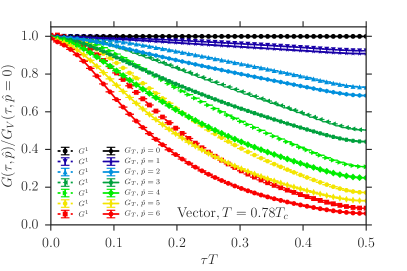
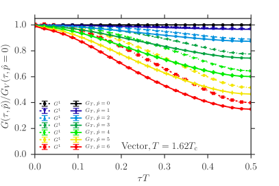
Figure 1: Momentum dependence of correlation functions for the vector channel, $G^{1}(\tau,\vec{p})$ and $G_{\rm T}(\tau,{p})$, normalized by the correlation function with zero momentum $G_{\rm V}({\tau},{0})$ for $T=0.78T_{\rm c}$ (upper) and $T=1.62T_{\rm c}$ (lower). The dashed and solid lines represent $G^{1}(\tau,\vec{p})$ and $G_{\rm T}(\tau,{p})$, respectively.

In this section, we show the numerical results. We first see the momentum dependence of the correlation functions. Figure 1 shows the correlation functions $G^{1}(\tau,\vec{p})$ and $G_{\rm T}(\tau,p)$ in the vector channel normalized by those with zero momentum,

$$G_{\rm V}(\tau,0)=\frac{1}{3}\sum_{i=1,2,3}G^{i}(\tau,\vec{0}),$$ (33)

for various values of $\hat{p}$ below and above $T_{\rm c}$. In the figure, the ratios $G^{1}(\tau,\vec{p})/G_{\rm V}(\tau,0)$ and $G_{\rm T}(\tau,p)/G_{\rm V}(\tau,0)$ are plotted by the dashed and solid lines, respectively. The errors in the figure are estimated for the ratios $G^{1}(\tau,\vec{p})/G_{\rm V}(\tau,0)$ and $G_{\rm T}(\tau,p)/G_{\rm V}(\tau,0)$ by the jackknife method; because of the strong correlation between correlation functions with different $p$, these errors are suppressed compared with those of the correlation functions themselves. The figure shows that the ratios $G^{1}(\tau,\vec{p})/G_{\rm V}(\tau,0)$ and $G_{\rm T}(\tau,p)/G_{\rm V}(\tau,0)$ become smaller as $p$ is increased. This behavior is consistent with Eqs. (5) and (9) because as $E(p)$ becomes larger, the contribution of the bound state to the correlation function is more suppressed. The figure also shows that $G^{1}(\tau,\vec{p})$ and $G_{\rm T}(\tau,p)$ behave differently even at $T=0.78T_{\rm c}$. As momentum become larger, the separation becomes more prominent with $G_{\rm T}(\tau,p)<G^{1}(\tau,\vec{p})$. As we discussed in Sec. II, $A_{\rm T}(\omega,\vec{p})=A_{\rm L}(\omega,\vec{p})=A_{\rm V}(P^{2})$ in the vacuum. From Eq. (16) we thus have

$$A_{\rm T}(\omega,p)=\frac{\omega^{2}-p^{2}}{\omega^{2}}A_{1}(\omega,\vec{p}).$$ (34)

Because the factor $(\omega^{2}-p^{2})/\omega^{2}$ is always smaller than unity, we have $A_{\rm T}(\omega,p)\leq A_{1}(\omega,\vec{p})$, which leads to $G_{\rm T}(\tau,p)\leq G^{1}(\tau,\vec{p})$. Similar behavior is observed for $T=1.62T_{\rm c}$.

V.2 Spectral function

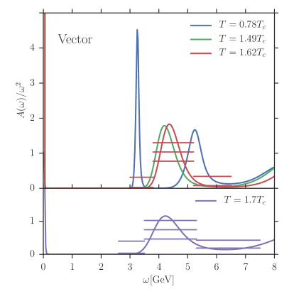
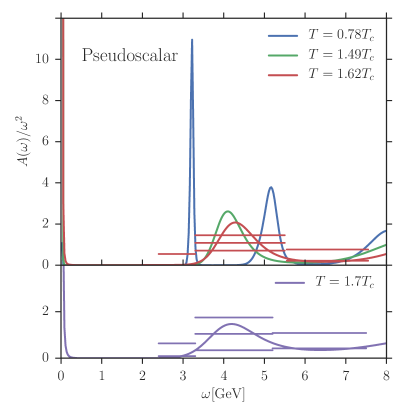
Figure 2: Spectral functions at $T/T_{\rm c}=0.78,~{}1.49,~{}1.62$, and $1.7$ at zero momentum. The upper and lower panels show the vector and pseudoscalar channels, respectively. The horizontal lines show the averages of the spectral functions for some ranges of $\omega$ and their errors at $T/T_{\rm c}=1.62$ and $1.70$.

Next, we analyze the $T$ dependence of the spectral functions with MEM and study the existence of the peaks corresponding to the $J/\psi$ and $\eta_{c}$ at finite temperature. The upper and lower panels of Fig. 2 show the spectral functions with zero momentum in the vector and pseudoscalar channels, respectively. The error bars for the average of the spectral function for some intervals of $\omega$ estimated by Eq. (27) are shown by three horizontal lines for $T/T_{\rm c}=1.62$ and $1.70$. The central lines show the averages of the spectral functions in the interval covered by the line, and the top and bottom ones indicate its $1\sigma$ error band. The result of the error analysis in the vector channel suggests that the peak corresponding to the $J/\psi$ exists at $T=1.62T_{\rm c}$ with probabilistic significance. On the other hand, for the pseudoscalar channel at $T=1.62T_{\rm c}$, the error for the peak structure corresponding to the $\eta_{c}$ has a small overlap with the error which is put for the right side valley of the structure. This shows that the plausibility of the existence of the peak is smaller than that for the vector channel. In other words, absence of the peak of $\eta_{c}$ at $T=1.62T_{\rm c}$ cannot be excluded by $1\sigma$.

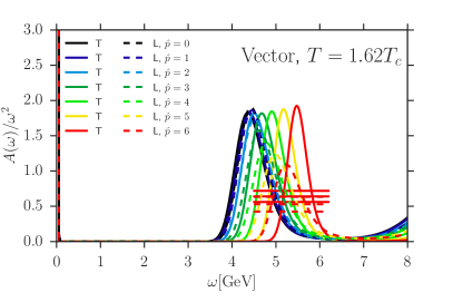
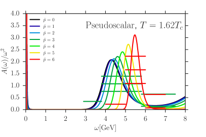
Figure 3: Momentum dependence of the spectral functions at $T=1.62T_{\rm c}$. The upper and lower panels show the vector and pseudoscalar channels, respectively. The error bars are shown for averages of the spectral functions for the vector channel at $\hat{p}=6$ and for the pseudoscalar channel at $\hat{p}=3$ and $6$.

In order to discuss the existence of the peak in the pseudoscalar channel at $T=1.62T_{\rm c}$ and the momentum dependence of the peaks, we next show the momentum dependence of the spectral functions in the vector and pseudoscalar channels at $T=1.62T_{\rm c}$ in the upper and lower panels in Fig. 3, respectively. In the upper panel, $A_{\rm T}(\omega,p)$ and $A_{\rm L}(\omega,p)$ are shown by the solid and dashed lines, respectively. In the lower panel, the errors for the peaks of the spectral functions in the pseudoscalar channel are shown for $\hat{p}=3$ and $6$. The lower panel suggests that the peak corresponding to the $\eta_{c}$ exists at $\hat{p}=3$ and $6$. The existence of the $J/\psi$ peak in the vector channel at nonzero momenta is also indicated from the upper panel. We thus suppose that the $J/\psi$ and $\eta_{c}$ survive up to $T=1.62T_{\rm c}$, which is a consistent result as in previous works Asakawa and Hatsuda (2004); Datta et al. (2004a), The possibility that the existence of the peak depends on $p$ for $T=1.62T_{\rm c}$, however, is not excluded in these analyses.

Figure 3 also shows that the peaks corresponding to the $J/\psi$ and $\eta_{c}$ are well isolated from the second structure in the spectral functions. This suggests that the dependence of $\bar{Z}(p)$ and $\bar{E}(p)$ on $\omega_{\rm max}$ is suppressed so that these quantities can be analyzed with small ambiguity.

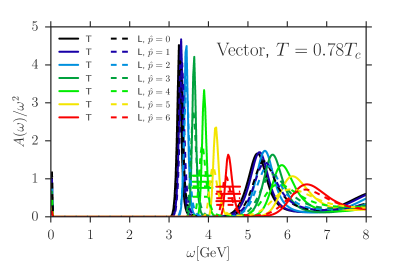
Figure 4: Momentum dependence of the spectral functions $A_{\rm T}(\omega,p)$ and $A_{\rm L}(\omega,p)$ in the vector channel at $T=0.78T_{\rm c}$. Errors for the average of the spectral functions are shown for $\hat{p}=4$ and $6$.

In Fig. 4, we show the momentum dependence of the spectral functions in the vector channel, $A_{\rm T}(\omega,p)$ and $A_{\rm L}(\omega,p)$, for $T=0.78T_{\rm c}$. To see the separation of the transverse and longitudinal channels, we show the errors for the averages of $A_{\rm T}(\omega,p)$ and $A_{\rm L}(\omega,p)$ with the same energy interval for $\hat{p}=4$ and $6$. From the figure, one observes that the spectral functions in the transverse and longitudinal channels agree with each other within the error. This result is consistent with the vacuum property of the spectral functions discussed in Sec. II. It, however, is worth emphasizing that this agreement is obtained although $A_{\rm T}(\omega,p)$ and $A_{\rm L}(\omega,p)$ are constructed from completely different correlation functions as shown in Fig. 1. From the upper panel in Fig. 3, one also finds that the degeneracy of $A_{\rm T}(\omega,p)$ and $A_{\rm L}(\omega,p)$ is observed even for $T=1.62T_{\rm c}$. This is a nontrivial result because these functions can behave differently because of the lack of Lorentz invariance.

V.3 Residue and dispersion relation

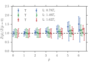
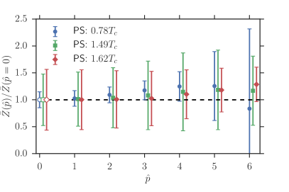
Figure 5: Ratio of the residues of the peaks, $\bar{Z}(p)/\bar{Z}(0)$, corresponding to the $J/\psi$ (upper) and $\eta_{c}$ (lower). The transverse (T) and longitudinal (L) components are shown in the upper panel.

Next, we turn to $\bar{Z}(p)$ and $\bar{E}(p)$. In Fig. 5, we show the momentum dependence of $\bar{Z}(p)$ obtained with Eq. (28) for the vector and pseudoscalar channels for $T/T_{\rm c}=0.78,~{}1.49,$ and $1.62$. In the figure, the normalized results, $\bar{Z}(p)/\bar{Z}(0)$, are plotted in order to see the momentum dependence of $\bar{Z}(p)$. The errors in the figure include only the one of the numerator of the ratio estimated by MEM. The figure shows that $\bar{Z}(p)$ does not have momentum dependence within the error for all the temperatures and all the channels for which we carried out analysis. This result is reasonable for $T/T_{\rm c}=0.78$, at which the medium effects should be well suppressed. Our analysis, however, show that $\bar{Z}(p)$ is insensitive to $p$ even at $T/T_{\rm c}=1.49$ and $1.62$, which is a nontrivial result.

We note that the errors of $\bar{Z}(p)/\bar{Z}(0)$ in Fig. 5 would be reduced if we take into account the correlation between $\bar{Z}(p)$ and $\bar{Z}(0)$. In order to estimate the correlation, however, one has to perform the MEM analysis for two different correlation functions in a single analysis. Because we perform the MEM analysis for individual momenta, this correlation cannot be estimated in our analysis.

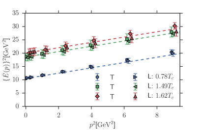
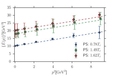
Figure 6: Dispersion relations $\bar{E}(p)$ of the $J/\psi$ (upper) and $\eta_{c}$ (lower) for $T/T_{\rm c}=0.78$, $1.49$, and $1.62$. The dashed lines indicate the vacuum dispersion relation Eq. (10) with $m=\bar{E}(0)$.

$T/T_{\rm c}$	$0.78$	$1.49$	$1.62$
$J/\psi$	$3.24(6)$	$4.30(16)$	$4.47(16)$
$\eta_{c}$	$3.19(5)$	$4.24(31)$	$4.49(48)$

Table 2: Masses of the ground states of the charmonia in the vector and pseudoscalar channels defined by $\bar{m}=\bar{E}(0)$.

To see the medium effects on the dispersion relation, we show the results on $\bar{E}(p)$ in Fig. 6. In the figure, we plot the square of this quantity $(\bar{E}(p))^{2}$ as a function of $p^{2}$, since this plot is convenient to see the deviation of $\bar{E}(p)$ from the vacuum dispersion relation Eq. (10). From the figure, one first observes that the masses of the charmonia, defined by $\bar{m}=\bar{E}(0)$, become larger as $T$ is increased. The values of $\bar{m}$ in the vector and pseudoscalar channels at $T/T_{\rm c}=0.78,~{}1.49,$ and $1.62$ are listed in Table 2. Although such a mass shift in MEM analyses were suggested in previous study Nonaka et al. (2011), our analysis confirms the medium effects on the mass of the charmonia with a quantitative error analysis for the first time.

In Fig. 6, the vacuum dispersion relation Eq. (10) with $m=\bar{m}$ is shown by the dashed lines. The figure shows that the functional form of $\bar{E}(p)$ is consistent with Eq. (10) within statistics even at $T/T_{\rm c}=1.49$ and $1.62$.

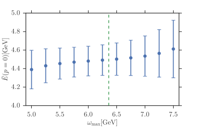
Figure 7: $\omega_{\rm max}$ dependence of $\bar{E}(p=0)$ for $N_{\tau}=46$ for the $J/\psi$ peak in the vector channel. The lower bound is fixed to $\omega_{\rm min}=3$ GeV. The vertical dashed line shows the local minimum between the first and second peaks.

In order to see the dependence of these results on the choice of the interval $I=[\omega_{\rm min},\omega_{\rm max}]$, in Fig. 7 we show the $\omega_{\rm max}$ dependence of $\bar{E}(p=0)$ for $N_{\tau}=46$ in the vector channel with $\omega_{\rm min}=3$ GeV. The value of $\omega_{\rm max}$ used in Fig. 6, i.e. the minimum of the spectral function between the first and second peaks, is shown by the vertical dashed line. The figure shows that the value and error of $\bar{E}(p)$ are insensitive to the choice of $\omega_{\rm max}$. In fact, the variation of the result with the change of $\omega_{\rm max}$ in $\pm 500$ MeV is about four times smaller than the error. The same conclusions holds also for the other cases and for $\bar{Z}(p)$. As discussed already in Sec. IV, the numerical results hardly change with the variation of $\omega_{\rm min}$. For example, when we choose the lower bound as $\omega_{\rm min}=2$ GeV, the numerical result overlaps with that in Fig. 7 within numerical precision. These results suggest that our analysis of $\bar{E}(p)$ is insensitive to the choice of the interval $I$ and thus is well justified.

The results in Figs. 5 and 6 suggest that the momentum dependence of the charmonia hardly changes from the Lorentz covariant one in Eqs. (9) and (10) even well above $T_{\rm c}$, although the rest mass $m$ is significantly increased as $T$ is raised. In vector channels, we do not observe difference between the transverse and longitudinal components within the error in MEM analysis even at finite temperature. These results are nontrivial because Lorentz symmetry is lost in medium, and quite interesting from the phenomenological points of view.

VI Conclusion

In this paper, we study the properties of charmonia at nonzero momentum in the vacuum and in medium with the lattice Euclidean correlation functions in the pseudoscalar and vector channels with MEM. The transverse and longitudinal components for the vector channel are analyzed separately. In addition to the standard analysis of spectral functions, we focus on the residue and dispersion relations for charmonia. To analyze these quantities with error in MEM, we have introduced the definitions in Eqs. (28) and (29). We have numerically checked that the peaks corresponding to the $J/\psi$ and $\eta_{c}$ can be studied by this analysis, as they are well isolated and the results are insensitive to the choice of the interval $I$.

In the vacuum, the dispersion relations for charmonia in all channels, pseudoscalar and vector, are consistent with the Lorentz covariant form and the residues for the bound states do not show the momentum dependence. In the vector channel, the peaks for the transverse and longitudinal components agree with each other within probabilistic significance. At finite temperature, we find the significant mass enhancement of charmonia as medium effects. On the other hand, the dispersion relations are consistent with that in the vacuum even at $T\simeq 1.6T_{\rm c}$ within probabilistic significance in MEM. Difference of the spectral functions between the transverse and longitudinal components in the vector channel is not observed. These results suggest an interesting observation that the medium effect on momentum dependence is well suppressed, although further improvement in statistics is required to obtain more accurate conclusion. We finally remark that these results cannot be explained by the naïve potential model. It is not explained by the threshold enhancement Mócsy and Petreczky (2008), either. These results suggest that the mass shift at finite temperature is caused by the nonperturbative interaction between charmonia and gluons in the medium.

Appendix A Failure of MEM analysis

As discussed in Sec. IV, in our MEM analysis we observed that the output spectral images behave in an unreasonable way in some channels and momenta on several sets of configurations. In this appendix, we discuss this problem in detail and show a criterion to remove them from the analysis.

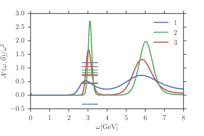
Figure 8: Reconstructed spectral images $A^{i}(\omega,\vec{0})$ with $i=1,~{}2$, and 3 and for $N_{\tau}=54$. The errors for the first peak in the spectral functions are measured at the same $\omega$ interval.

Let us first specify the problem. In Fig. 8, we show the spectral functions in the vector channel at zero momentum $A^{i}(\omega,\vec{p}=0)$ obtained by MEM for $i=1,~{}2$, and $3$ with $N_{\tau}=54$ ($T=1.38T_{\rm c}$). Because of rotational symmetry, these three spectral functions have to degenerate. Moreover, since our analysis discussed in Sec. V.2 shows the existence of a peak corresponding to the $J/\psi$ at $T/T_{\rm c}=1.49$ and $1.62$, the spectral function for $T=1.38T_{\rm c}$ should also have the peak. In Fig. 8, we indeed observe the peak in $A^{2}(\omega,\vec{0})$ and $A^{3}(\omega,\vec{0})$. The peak, however, is not observed in $A^{1}(\omega,\vec{0})$. This result shows that the reconstruction of the spectral image in MEM does not work well for $A^{1}(\omega,\vec{0})$. In the figure, the errors for the averages of $A^{i}(\omega,\vec{0})$ around the $J/\psi$ peak are also shown. The result shows that the averages for all channels agree with one another within the error, although the error for $A^{1}(\omega,\vec{0})$ is large. In this sense, the MEM analysis gives the consistent results for these three channels. It, however, seems obvious from the figure that the MEM analysis for $A^{1}(\omega,\vec{0})$ is not working well compared with the other two channels.

We observed this kind of unstable results in some channels and momenta for $N_{\tau}=48$ and $54$. We have checked that the increase of statistics does not always resolve this problem; this problem sometimes manifests itself when the number of gauge configurations is increased. We have also checked that this problem does not come from the finite numerical precision in our MEM code by confirming that the same problem shows up even if we change the numerical precision in our code from double to quadruple. It has been also checked that the change of the default model does not cure this problem.

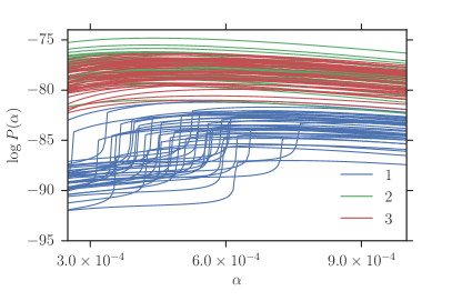
Figure 9: $\alpha$ dependence of $P^{i}(\alpha)$ with $i=1,2,$ and $3$. The results are shown for $25$ jackknife samples for each $i$. The reference point of the vertical axis is arbitrary.

We found that when the output spectral image shows an unstable behavior, the probability $P(\alpha)$ in Eq. (24) behaves pathologically as a function of $\alpha$. In Fig. 9, we show the probabilities $P^{i}(\alpha)$ for the three channels corresponding to the results in Fig. 8. In the figure, $P^{i}(\alpha)$ is shown for $25$ jackknife samples, i.e. the results for $25$ sets of configurations in which $1/25$ succeeding configurations are removed from the total configurations. From the figure, one finds that $P^{1}(\alpha)$ has an almost discontinuous kink structure while $P^{2}(\alpha)$ and $P^{3}(\alpha)$ behave smoothly as a function of $\alpha$. The figure also shows that the existence of the kink is robust against the small variation of the set of gauge configurations. We found that when $P(\alpha)$ has such kink structures, the output spectral image behaves in an unstable way as in $A^{1}(\omega,\vec{p})$ in Fig. 8.

At present, we have not clarified the origin of this pathological behaviors. One possibility for the origin of this behavior is the numerical precision of the lattice simulation and correlation functions. The numerical simulations, however, have been performed in double precision and it is difficult to alter the precision.

The pathological behavior of $P(\alpha)$ is observed on the analysis for $N_{\tau}=54$ and $48$, while we do not observe it for $N_{\tau}=96,~{}50,~{}46$, and $44$. In our study, we simply exclude the results of $N_{\tau}=54$ and $48$ from our analysis and concentrate on the other four $N_{\tau}$ values, which do not have the problem.

References

- Brambilla et al. (2011) N. Brambilla et al., Eur. Phys. J. C 71, 1 (2011), arXiv:1010.5827 [hep-ph] .
- Andronic et al. (2016) A. Andronic et al., Eur. Phys. J. C 76, 1 (2016), arXiv:1506.03981 [nucl-ex] .
- Matsui and Satz (1986) T. Matsui and H. Satz, Physics Letters B 178, 416 (1986).
- Hashimoto et al. (1986) T. Hashimoto, O. Miyamura, K. Hirose, and T. Kanki, Phys. Rev. Lett. 57, 2123 (1986).
- Akamatsu et al. (2009) Y. Akamatsu, T. Hatsuda, and T. Hirano, Phys. Rev. C 79, 054907 (2009), arXiv:0809.1499 [hep-ph] .
- PHENIX Collaboration et al. (2009) PHENIX Collaboration et al., Phys. Rev. Lett. 103, 082002 (2009), arXiv:0903.4851 [hep-ex] .
- Asakawa and Hatsuda (2004) M. Asakawa and T. Hatsuda, Phys. Rev. Lett. 92, 012001 (2004), arXiv:hep-lat/0308034 [hep-lat] .
- Datta et al. (2004a) S. Datta, F. Karsch, P. Petreczky, and I. Wetzorke, Phys. Rev. D 69, 094507 (2004a), arXiv:hep-lat/0312037 [hep-lat] .
- Umeda et al. (2004) T. Umeda, K. Nomura, and H. Matsufuru, Eur. Phys. J. C 39, 9 (2004), arXiv:hep-lat/0211003 [hep-lat] .
- Datta et al. (2005) S. Datta, F. Karsch, P. Petreczky, and I. Wetzorke, J. Phys. G: Nucl. Part. Phys. 31, S351 (2005), arXiv:hep-lat/0412037 [hep-lat] .
- Jakovác et al. (2007) A. Jakovác, P. Petreczky, K. Petrov, and A. Velytsky, Phys. Rev. D 75, 014506 (2007), arXiv:hep-lat/0611017 [hep-lat] .
- Umeda (2007) T. Umeda, Phys. Rev. D 75, 094502 (2007), arXiv:hep-lat/0701005 [hep-lat] .
- WHOT-QCD Collaboration et al. (2011) WHOT-QCD Collaboration, H. Ohno, S. Aoki, S. Ejiri, K. Kanaya, Y. Maezawa, H. Saito, and T. Umeda, Phys. Rev. D 84, 094504 (2011), arXiv:1104.3384 [hep-lat] .
- Ding et al. (2012) H.-T. Ding, A. Francis, O. Kaczmarek, F. Karsch, H. Satz, and W. Soeldner, Phys. Rev. D 86, 014509 (2012), arXiv:1204.4945 [hep-lat] .
- Borsányi et al. (2014) S. Borsányi et al., J. High Energ. Phys. 2014, 1 (2014), arXiv:1401.5940 [hep-lat] .
- Jarrell and Gubernatis (1996) M. Jarrell and J. E. Gubernatis, Physics Reports 269, 133 (1996).
- Asakawa et al. (2001) M. Asakawa, Y. Nakahara, and T. Hatsuda, Progress in Particle and Nuclear Physics 46, 459 (2001), arXiv:hep-lat/0011040 [hep-lat] .
- Datta et al. (2004b) S. Datta, F. Karsch, P. Petreczky, S. Wissel, and I. Wetzorke, arXiv:hep-lat/0409147 [hep-lat] (2004b), .
- Nonaka et al. (2011) C. Nonaka, M. Asakawa, M. Kitazawa, and Y. Kohno, J. Phys. G: Nucl. Part. Phys. 38, 124109 (2011).
- Oktay and Skullerud (2010) M. B. Oktay and J. I. Skullerud, arXiv:1005.1209 [hep-lat] (2010), .
- Aarts et al. (2013) G. Aarts, C. Allton, S. Kim, M. P. Lombardo, M. B. Oktay, S. M. Ryan, D. K. Sinclair, and J.-I. Skullerud, J. High Energ. Phys. 2013, 1 (2013), arXiv:1210.2903 [hep-lat] .
- Ding (2013) H.-T. Ding, Nuclear Physics A The Quark Matter 2012 Proceedings of the XXIII International Conference on Ultrarelativistic Nucleus‒Nucleus Collisions, 904–905, 619c (2013), arXiv:1210.5442 [nucl-th] .
- Liu et al. (2007) H. Liu, K. Rajagopal, and U. A. Wiedemann, Phys. Rev. Lett. 98, 182301 (2007), arXiv:hep-ph/0607062 [hep-ph] .
- Bellac (2000) M. L. Bellac, Thermal Field Theory, revised.版 ed. (Cambridge University Press, 2000).
- Shuryak (1990) E. V. Shuryak, Phys. Rev. D 42, 1764 (1990).
- Pisarski and Tytgat (1996) R. D. Pisarski and M. Tytgat, Phys. Rev. D 54, R2989 (1996), arXiv:hep-ph/9604404 [hep-ph] .
- Van Hove (1953) L. Van Hove, Phys. Rev. 89, 1189 (1953).
- Braaten et al. (1990) E. Braaten, R. D. Pisarski, and T. C. Yuan, Phys. Rev. Lett. 64, 2242 (1990).
- Kitazawa et al. (2014) M. Kitazawa, T. Kunihiro, and Y. Nemoto, Phys. Rev. D 89, 056002 (2014), arXiv:1312.3022 [hep-ph] .
- Kim et al. (2015) T. Kim, M. Asakawa, and M. Kitazawa, Phys. Rev. D 92, 114014 (2015), arXiv:1505.07195 [nucl-th] .
- Kapusta and Gale (2006) J. I. Kapusta and C. Gale, Finite-temperature field theory: principles and applications. (Cambridge University Press, 2006).
- Bryan (1990) R. K. Bryan, Eur Biophys J 18, 165 (1990).
- Aarts et al. (2007) G. Aarts, C. Allton, J. Foley, S. Hands, and S. Kim, Phys. Rev. Lett. 99, 022002 (2007), arXiv:hep-lat/0703008 .
- Mócsy and Petreczky (2008) Á. Mócsy and P. Petreczky, Phys. Rev. D 77, 014501 (2008), arXiv:0705.2559 [hep-ph] .