Accelerating Hartree–Fock exchange calculation using
the TURBOMOLE program system:
different techniques for different purposes

Abstract

Hartree–Fock theory is one of the most ancient methods of computational chemistry, but up to the present day quantum chemical calculations on Hartree–Fock level or with hybrid density functional theory can be excessively time consuming.

We compare three currently available techniques to reduce the computational demands of such calculations in terms of timing and accuracy.

I Introduction

Hartree–Fock (HF) as an autonomous quantum chemical level of theory is nowadays hardly in use anymore, but still it remains one of the most applied methods, because it serves as reference wave function for post–HF methods like Møller–Plesset perturbation theory (MP2, MP3, …) or Coupled–Cluster calculations (CC2, CCSD, CCSD(T), …). Also, density functional theory (DFT) makes use of a HF-like method in the computation of hybrid functionals like the popular B3-LYP or PBE0. The evaluation of HF exchange is the time determining operation in such a hybrid DFT calculation. In modern implementations of MP2 energy calculations the HF part often takes significantly longer than the MP2 part.

Several techniques to reduce the computational costs are available on the market, e.g. applying integral screeningHäser and Ahlrichs (1989); Ochsenfeld et al. (1998), exploitation of the resolution–of–the–identityWeigend (2002); Kattannek (2006) (RI), and using pseudospectralFriesner (1985) or seminumerical methodsNeese et al. (2009); Plessow and Weigend (2012).

There is some confusion among users about which method is the appropriate one for their specific problem. In this piece of writing, we summarize the efficiency and accuracy of available techniques and aim to provide some guidance for their usage.

II Computational background

Hartree-Fock (HF) became applicable for scientific computing around 1950 due to the works of C. C. J. RoothaanRoothaan (1951) and G. G. HallHall (1951) and the introduction of spacial basis functions like those of Gaussian-type by BoysBoys (1950). The Roothaan–Hall self-consistent field method (SCF) equation is

$$FC=SC\epsilon,$$ (1)

$F$ is the Fock matrix, $S$ is the overlap matrix, $C$ are the expansion coefficients for the molecular orbitals (MOs), and $\epsilon$ is a diagonal matrix with orbital energies. The Fock matrix can be separated in the Coulomb part $J$ and the exchange part $K$. The SCF equation is solved iteratively, until the energy is minimized to convergence. $J$ and $K$ can be evaluated hereby either in shared or in separated loops over basis functions. If they are calculated separately, the $J$ part can be solved very efficiently using special techniques, e.g. with the multipole accelerated RI-$J$ (MARI-$J$) approach.Sierka et al. (2003) That leaves the $K$ part to be optimized.

Approximations

The formal scaling of the two-electron, four center integrals which build up both the $J$ and $K$ part of the Fock matrix is $N^{4}$, with $N$ being the total number of atom centered basis functions (see below). Already direct SCF procedures with a common evaluation of $J$ and $K$ can be speeded up significantly and their asymptotic scaling can be reduced to $N^{2}$ by applying two–electron integral screeningHäser and Ahlrichs (1989). The convergence can be accelerated by the use of minimized density differences or direct inversion in the iterative subspace (DIIS).Pulay (1980) Integral screening and related techniques are generally used wherever applicable, since the mathematically sound deployment of upper bounds for the integrals do not introduce any noticeable numerical errors. While for smaller structures the formal scalings remains $N^{4}$, the situation gets better the bigger the molecules become - depending on the size and diffuseness of the chosen basis set (see Table 1).

Table 1: Scaling behaviour of the time-demanding steps in a HF or hybrid DFT calculation

	formal scaling $\rightarrow$	asymptotic scaling
2-e integrals ($J$ and $K$)	$N^{4}$	$N^{2}$
( RI-$J$ instead of $J$	$N^{3}$	$N^{2}$ )
( MARI-$J$ instead of $J$	$N^{3}$	$N$ )
DFT quadrature	$N^{3}$	$N$
Matrix diagonalization	$N^{3}$	$N^{3}$

We refer to the results from such calculations as exact HF solution, because no approximation is used, only integrals are neglected that do not contribute.

rij

If the RI approximation is being used for the Coulomb part $J$, the operator can be replaced:

$$J_{\nu\mu}\sim J_{\nu\mu}^{RI}\qquad;\qquad K_{\nu\mu}=K_{\nu\mu}^{screened}.$$ (2)

The $K$ part can be re-ordered for an exact optimum–screened procedureKattannek (2006) which is similar to a linear scaling procedure as described by Ochsenfeld et al.Ochsenfeld et al. (1998). This introduces an RI error in $J$ but not in $K$. This approach will be denoted rij in the following.

rik

The RI approximation can also be used to fully replace the exchange part:Weigend (2002)

$$J_{\nu\mu}\sim J_{\nu\mu}^{RI}\qquad;\qquad K_{\nu\mu}\sim K_{\nu\mu}^{RI}.$$ (3)

The same Coulomb operator as above from Eq.2 is used. This approach will be denoted rik in the following. (One can also call it rijk, but the $J$ part is not crucial here.)

senex

In the approach denoted senex in the following, again the Coulomb operator from Eq.2 is used while the evaluation of $K$ is now done by solving one integral analytically and the other one numerically on a spacial grid:Plessow and Weigend (2012)

$$J_{\nu\mu}\sim J_{\nu\mu}^{RI}\qquad;\qquad K_{\nu\mu}\sim K_{\nu\mu}^{SN}.$$ (4)

This is a seminumerical procedure that can be done with the same grids on which the density functionals are evaluated.

Basis sets and auxiliary basis sets

The introduction of linear combination of atomic orbitals (LCAO) as approximation of one-electron wave functions was a fundamental step for practical calculations. The development of general applicable basis sets made model chemistry reproducible and revisable. Yet, a steady and on-going development created a whole zoo of basis sets inhibited by an enormous amount of abbreviations, lots of them only understandable by experts. At the EMSL Basis Set Exchange (https://bse.pnl.gov/bse/portal) the most frequently used ones can be obtained ready to use in different input formats.

Different recommendations can be given for DFT and wave function theories (WFT). For DFT, already relatively small basis sets often yield decent results. To benchmark their performance, we use def-SV(P)Schäfer et al. (1992) and def-TZVPSchäfer et al. (1994) as typical representatives. For an improved quantitative description - especially when dealing with heavy element compounds -, we rather suggest to use the def2 basis setsWeigend and Ahlrichs (2005), though. def-SV(P) is a split valence basis set with one set of polarization functions for the non-hydrogen atoms. It is of comparable size and quality as the Pople 6-31G*Hariharan and Pople (1973) basis set. def-TZVP is a triple-$\zeta$ basis set with one set of uncontracted polarization functions. This is comparable to the 6-311G**Krishnan et al. (1980) basis set.

Wave function theory is not only more expensive in terms of computational time, but also much more demanding concerning the basis set. Heavily polarized triple- and quadruple-$\zeta$ basis sets def2-TZVPP and def2-QZVPPWeigend and Ahlrichs (2005) as typical representatives will be used in the following sections. Those are comparable to Dunnings cc-pVTZ and cc-pVQZ.Dunning (1989) Additional diffuse basis functions are required when studying anions or properties related to electron densities not localized close to the atoms. We use def2-TZVPPDRappoport and Furche (2010) for such a basis set. The suffix D indicates the diffuse functions here, as the + is for the Pople type basis sets and the prefix aug- for the ones of Dunning type.

The prefixes def- and def2- for the basis set will be skipped in the following, because the names are unambiguous for the elements computed in this work.

The SVP, TZVP and QZVP basis set family combines several benefits which make them usable for almost all applications – namely the fact that they are available for all elements, automatically include ECPs for heavier elements to include scalar relativistic effects. Furthermore, when applying the RI approximation, special auxiliary basis sets are needed. For the used basis sets optimized auxiliary basis sets are available for RI-J, RI-K and correlated RI calculations like RI-MP2, RI-CC2, RI-CCSD, etc. They are optimized and investigated for $J^{RI}$ in Ref. Weigend, 2006 and for the common usage in $J^{RI}$ and $K^{RI}$ in Ref. Weigend, 2008. All TURBOMOLE basis sets and auxilary basis sets can be found online: http://www.cosmologic.de/basis-sets/basissets.php

III Benchmark calculations

All calculations have been performed using TURBOMOLE V6.4.TM The exact HF SCF calculations were done with the dscf module. The approximated HF approaches are implemented in the ridft module. (Despite of its name it can also perform non–DFT calculations.) Default settings were used throughout if not specified otherwise.

As benchmark sets, amylose-chains containing one (24 atoms), two (45 atoms), and four (87 atoms) D-glucose unitsKussmann and Ochsenfeld (2007) and arsenic clusters As_n (n=4,8,12)Furche et al. (2014) were selected. $C_{1}$ symmetry was used in the computations. For atomization energy tests, the structures of methane, ethane, propane, and butane were optimized on BP/SV(P) level.

Accuracy

The differences (RI and seminumerical errors) between exact HF energies (using dscf) and the approximated HF energies (using ridft) are collected in Table 2 for the different amylose-chains with the different basis sets.

Table 2: The RI and seminumerical errors per atom of amylose chains in $\mu$Hartree. na is the number of atoms, nbf the number of CAO basis functions.

	na	nbf	rij	rik	senex
SV(P)
	24	204	146	-21	151
	45	389	149	-21	173
	87	759	150	-21	167
TZVP
	24	312	159	-10	129
	45	592	160	-10	167
	87	1152	160	-10	143
TZVPP
	24	612	31	-12	-9
	45	1158	30	-12	23
	87	2250	29	-12	-3
TZVPPD
	24	750	31	-12	-13
	45	1418	29	-12	16
	87	2754	29	-12	-11
QZVPP
	24	1284	31	-14	-51
	45	2426	29	-14	-38
	87	4710	29	-14	-58

rij and rik yield errors of the same size for all molecules with a specific basis set. This leads to an error cancellation when reactions are studied. The errors of senex are as small as the RI errors, but they are not systematic for different molecular sizes. This behavior is illustrated in Fig. 1. Thus, for senex no such error cancellation can be expected.

Figure 1: The RI and seminumerical errors per atom in $\mu$Hartree for 1, 2, and 4 glucose units with the different basis sets. nbf is the number of CAO basis functions.

To get an impression of such error cancellation, atomization energies of small alkanes have been calculated on HF, MP2, CCSD(T), and B3-LYP level using the cc-pVTZ basis set. The frozen core approximation was used in the correlated calculations. In Table 3 the differences (RI and seminumerical errors) between calculations using a reference wave function from dscf and from ridft with the different approximations is shown.

Table 3: The RI and seminumerical errors in calculations of atomization energies of alkanes using the cc-pVTZ basis set in kcal/mol.

molecule	approximation	HF	MP2	CCSD(T)	B3-LYP
methane	rij	-0.06	-0.06	-0.07	-0.07
	rik	0.00	0.00	0.00	0.00
	senex, m1	-1.03	-1.94	-0.65	-0.05
	senex, m3	-1.17	-1.97	-0.74	-0.08
	senex, m5	-0.06	-0.06	-0.06	-0.08
ethane	rij	-0.09	-0.08	-0.09	-0.10
	rik	0.00	0.00	0.00	-0.01
	senex, m1	-2.27	-3.92	-1.42	-0.10
	senex, m3	-2.30	-3.92	-1.45	-0.11
	senex, m5	-0.09	-0.08	-0.09	-0.11
propane	rij	-0.12	-0.11	-0.12	-0.13
	rik	0.00	0.00	0.00	-0.01
	senex, m1	-3.39	-6.18	-2.24	-0.14
	senex, m3	-3.44	-5.85	-2.15	-0.15
	senex, m5	-0.12	-0.11	-0.12	-0.15
butane	rij	-0.15	-0.14	-0.15	-0.17
	rik	0.00	0.01	0.01	-0.01
	senex, m1	-4.72	-8.47	-3.20	-0.25
	senex, m3	-4.58	-7.80	-2.87	-0.19
	senex, m5	-0.15	-0.14	-0.15	-0.19

The calculation of atomization energies is known to be prone to insufficiencies of the basis set as well as of the method itself, since all errors sum up. It can be seen that the errors introduced by the RI approximation are well–behaved, the rik errors being an order of magnitude smaller than the ones from rij due to the larger auxiliary basis set of rik which is used for both $J$ and $K$ part of a rik calculation. The errors of senex with the default grid (m1) are noticeable larger and quickly increasing with the system size. Grids of the m5 size have to be used to reach the accuracy of rij. This is a consequence of the irregular patterns recognizable in Table 2.

A comparison between the different methods shows an interesting effect. On MP2 level the errors are larger than on HF level, while they are smaller on CCSD(T) level. It can be assumed that applying perturbation theory on an imprecise wave function increases its deficits, whereas the iterative solution of the CCSD equation repairs some of them.

The situation looks more relaxed when using hybrid-DFT rather than pure HF. In the last column of the table the values for the B3-LYP functional (using 20% HF exchange) are collected. The RI errors are of the same magnitude as for HF and already with small grids the seminumerical errors are acceptable.

Timings

In Table 4 the wall-times in minutes are collected for the different approximations, basis sets, and system sizes of amylose chains. In Fig. 2 the data is plotted.

Table 4: The wall-time in minutes for HF calculations of amylose chains. The SCF was started from an extended Hückel guess. In all cases, the number of SCF iterations in the same row was identical. na is the number of atoms, nbf the number of CAO basis functions.

							fudged
	na	nbf	dscf	rij	rik	senex	rik
SV(P)
	24	204	1.9	1.7	2.3	5.7	2.3
	45	389	10.8	8.1	24.9	27.7	24.9
	87	759	53.1	30.0	298.5	101.0	99.5
TZVP
	24	312	8.8	7.3	4.6	11.8	4.6
	45	592	53.9	37.8	42.1	58.6	42.1
	87	1152	269.2	156.3	584.7	224.0	146.2
TZVPP
	24	612	53.3	39.4	12.0	27.7	12.0
	45	1158	296.6	188.4	103.6	133.9	103.6
	87	2250	1403.9	737.6	1447.4	487.6	180.9
TZVPPD
	24	750	159.7	121.5	16.3	40.9	16.3
	45	1418	1206.7	859.9	164.3	225.4	82.2
	87	2754	7427.1	4506.8	3162.6	908.8	316.3
QZVPP
	24	1284	582.8	388.9	33.9	98.3	33.9
	45	2426	3133.3	1808.3	427.7	470.3	142.6
	87	4710	15920.4	7043.1	8456.7	1643.3	497.5

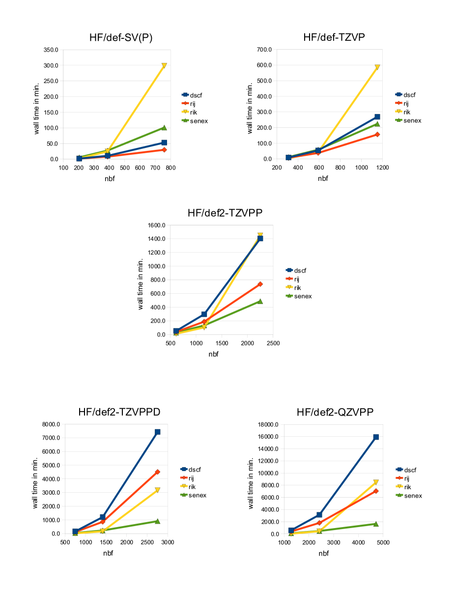
Figure 2: The computational wall-time in minutes for 1, 2, and 4 glucose units with the different basis sets. nbf is the number of CAO basis functions.

rij always performs better than dscf. For the typical DFT basis sets SV(P) and TZVP, it is the fastest and the curve will stay under the others when going to even larger systems due to its scaling. For larger basis sets rik is faster for small and medium sized systems, but rij can pass by on larger systems.

The performance of rik is very good for TZVPP basis sets or larger, as long as everything fits in memory. But performance goes down due to the need of blocking – if the memory given is insufficient, the algorithm has to redo the same loops for several batches into which the whole problem has been divided. For the computations a maximum memory ($ricore) of 2GB was chosen. The additional column denoted fudged rik in Table 4 is a hypothetical timing, calculated as if enough memory were available such that only one batch would be sufficient. It can be seen that the blocking is the main reason that the performance drops for larger systems. Since more and more memory is available in off–the–shelf computers, rik will become more and more fetching in future applications.

senex with the m1 grid is very fast for basis sets of TZVPP size and larger. Especially, for bigger systems one has to admit that the performance looks impressive.

Heavier elements, truncated RI, and semi-direct dscf

When studying compounds composed of elements beyond the realms of organic chemistry, the trends and characteristics can be recognized already with smaller systems. We use arsenic cluster to benchmark the performance of heavier atoms. The timings are collected in Table 5. The advantage of rik when using large basis sets over dscf and rij diminishes for these systems compared to the amylose chains. The performance behavior of the other approaches is quite similar to the former cases.

Two additional columns are presented here. One with timings of semi-direct SCF as an option of dscf and the other with timings of truncated RI as an option of rik. In the semi-direct dscf mode, the most time consuming and frequently used integrals are stored on disk. The semi-direct mode is for smaller systems a bit faster than the fully direct mode, but the situation changes for larger problems.

In truncated RI procedures reduced auxiliary basis sets are used during SCF iterations. The final SCF iteration is computed with the full auxiliary basis set. Usually, functions with the two highest $l$-quantum numbers are skipped. For rij and senex this will be not efficient, since it would only affect the $J$ part and it is, furthermore, not compatible with MARI-$J$. The error of the truncation is by orders of magnitudes smaller than the RI error on HF energies, but can increase the error of post-HF calculations, see Ref. Weigend, 2002.

Table 5: The wall-time in minutes for HF calculations of arsenic cluster As_n (n=4,8,12). The SCF was started from extended Hückel guess. In all cases, the number of SCF iterations in the same row was identical. na is the number of atoms, nbf the number of CAO basis functions.

							fudged	semi-direct	trunc.
	na	nbf	dscf	rij	rik	senex	rik	dscf	rik
SV(P)
	4	140	0.7	0.7	1.8	1.2	1.8	0.3	1.7
	8	280	5.5	4.7	23.5	6.9	23.5	3.1	22.0
	12	420	17.7	13.7	122.9	23.0	61.5	11.2	119.5
TZVP
	4	156	1.5	1.4	2.1	1.6	2.1	0.5	2.5
	8	312	12.2	9.8	29.7	10.3	29.7	6.0	25.9
	12	468	34.9	25.1	135.3	30.1	67.7	20.4	121.0
TZVPP
	4	220	3.8	3.3	3.3	2.4	3.3	1.8	2.9
	8	440	37.8	28.9	50.4	20.0	50.4	52.5	47.0
	12	660	105.7	75.4	212.7	53.7	70.9	106.5	186.5
TZVPPD
	4	248	5.7	5.1	3.6	3.0	3.6	3.0	3.6
	8	496	66.4	51.0	57.7	25.3	57.7	70.7	56.1
	12	744	220.1	158.0	244.4	67.1	81.5	203.2	224.8
QZVPP
	4	444	37.3	29.8	8.6	9.3	8.6	22.4	7.7
	8	888	317.0	226.1	106.6	57.9	53.3	315.9	102.5
	12	1332	1071.3	656.4	638.4	194.7	159.6	1093.6	588.5

IV Conclusion

rij is in almost all cases the better choice than plain dscf. One exception could come up for really large systems, somewhere beyond 20000 basis functions. Here, the memory demands of RI could be a limiting factor. However, at the moment such calculations are not yet feasible except for single-point energy calculations.

rik is a good choice for small to medium sized molecules with large basis set, especially with diffuse functions. A typical scenario is a MP2 calculation in which HF is the most time consuming part, e.g. in a RI-MP2 energy calculation of glucose with def2-TZVPPD with the ricc2 module and a reference wave function from dscf, the HF part take 98% of the overall run time.

From a pessimistic point of view, one could say that senex is not fast enough for typical DFT applications with small basis sets and not accurate enough for typical WFT applications with large basis sets. More optimistically one has to say, that hybrid–DFT with large basis sets or two–component relativistic hybrid–DFT of larger system are becoming accessible through this.

The semi-direct mode of dscf introduces no additionali error, but it is for larger systems not faster than the direct mode. Also, it has to be noted that the semi-direct mode leads to additional I/O. The truncated rik is always faster than full rik, yet not really significantly. It can be of use in hybrid–DFT calculations, but the small gain timing does hardly outweigh the loss of precision to make it a good choice for WFT applications.

As general remark it should be pointed out, that one must not mix calculations with different approximations. In one coherent investigations all systems have to be treated in the same way.

References

- Häser and Ahlrichs (1989) M. Häser and R. Ahlrichs, J. Comput. Chem. 10, 104 (1989).
- Ochsenfeld et al. (1998) C. Ochsenfeld, C. A. White, and M. Head-Gordon, J. Chem. Phys. 109, 1663 (1998).
- Weigend (2002) F. Weigend, Phys. Chem. Chem. Phys. 4, 4285 (2002).
- Kattannek (2006) M. Kattannek, Ph.D. thesis, Fakultät für Chemie und Biowissenschaften, Universität Karlsruhe (TH) (2006).
- Friesner (1985) R. A. Friesner, Chem. Phys. Lett. 116, 39 (1985).
- Neese et al. (2009) F. Neese, F. Wennmohs, A. Hansen, and U. Becker, Chem. Phys. 356, 98 (2009).
- Plessow and Weigend (2012) P. Plessow and F. Weigend, J. Comput. Chem. 33, 810 (2012).
- Roothaan (1951) C. C. J. Roothaan, Rev. Mod. Phys. 23, 69 (1951).
- Hall (1951) G. G. Hall, Proc. R. Soc. Lond. A 205, 541 (1951).
- Boys (1950) S. F. Boys, Proc. R. Soc. Lond. A 200, 542 (1950).
- Sierka et al. (2003) M. Sierka, A. Hogekamp, and R. Ahlrichs, J. Chem. Phys. 118, 9136 (2003).
- Pulay (1980) P. Pulay, Chem. Phys. Lett. 73, 393 (1980).
- Schäfer et al. (1992) A. Schäfer, H. Horn, and R. Ahlrichs, J. Chem. Phys. 97, 2571 (1992).
- Schäfer et al. (1994) A. Schäfer, C. Huber, and R. Ahlrichs, J. Chem. Phys. 100, 5829 (1994).
- Weigend and Ahlrichs (2005) F. Weigend and R. Ahlrichs, Phys. Chem. Chem. Phys. 7, 3297 (2005).
- Hariharan and Pople (1973) P. C. Hariharan and J. A. Pople, Theor. Chem. Acc. 28, 213 (1973).
- Krishnan et al. (1980) R. Krishnan, J. S. Binkley, R. Seeger, and J. A. Pople, J. Chem. Phys. 72, 650 (1980).
- Dunning (1989) T. H. Dunning, J. Chem. Phys. 90, 1007 (1989).
- Rappoport and Furche (2010) D. Rappoport and F. Furche, J. Chem. Phys. 133, 134105 (2010).
- Weigend (2006) F. Weigend, Phys. Chem. Chem. Phys. 8, 1057 (2006).
- Weigend (2008) F. Weigend, J. Comput. Chem. 29, 167 (2008).
-
(22)
TURBOMOLE V6.4 2012, a development of University of
Karlsruhe and Forschungszentrum Karlsruhe GmbH, 1989-2007, TURBOMOLE
GmbH, since 2007; available from
http://www.turbomole.com. - Kussmann and Ochsenfeld (2007) J. Kussmann and C. Ochsenfeld, J. Chem. Phys. 127, 054103 (2007).
- Furche et al. (2014) F. Furche, R. Ahlrichs, C. Hättig, W. Klopper, M. Sierka, and F. Weigend, WIREs Comput Mol Sci 4, 91 (2014).