Bursts of activity in collective cell migration

Abstract

Dense monolayers of living cells display intriguing relaxation dynamics, reminiscent of soft and glassy materials close to the jamming transition, and migrate collectively when space is available, as in wound healing or in cancer invasion. Here we show that collective cell migration occurs in bursts that are similar to those recorded in the propagation of cracks, fluid fronts in porous media and ferromagnetic domain walls. In analogy with these systems, the distribution of activity bursts displays scaling laws that are universal in different cell types and for cells moving on different substrates. The main features of the invasion dynamics are quantitatively captured by a model of interacting active particles moving in a disordered landscape. Our results illustrate that collective motion of living cells is analogous to the corresponding dynamics in driven, but inanimate, systems.

Introduction

Collective cell movement depends on intracellular biological mechanisms as well as environmental cues due to the extracellular matrix (ECM)[1, 2, 3, 4, 5], mainly composed by collagen which is organized in hierarchical structures, such as fibrils and fibers. The mechanical properties of collagen fibril networks are essential to offer little resistance and high sensitivity to small deformations, allowing easy local remodeling and strong strain stiffening needed to ensure cell and tissue integrity [6]. Wound healing is a typical biological assay to study collective migration of cells under controlled conditions in vitro and is a prototypical experimental method to study active matter [7, 8, 9, 10]. Experiments performed on soluble collagen [11] or other gels [12], micro-patterned [13, 14] and deformable substrates [1] show that cell migration is guided by the substrate structure and stiffness [15, 5, 16].

It has been argued that collective migration properties arise from stresses transmitted between neighboring cells [1] giving rise to long-ranged stress waves in the monolayer [17, 18]. Hence the dynamics of an invading cell sheet is ruled by a combination of long-range internal stresses and interactions with the substrate, suggesting an analogy with driven elastic systems moving in a disordered medium such as cracks lines [19, 20], imbibition fronts [21] or ferromagnetic domain walls [22]. The scaling laws in these systems are usually associated with a depinning critical point that has been widely studied by simple models for interface dynamics. Thanks to a combination of numerical simulations [23, 24] and renormalization group theory [25, 23, 26, 27], we now have a detailed picture of the non-equilibrium phase transitions and universality classes in these systems. Here we substantiate the analogy between collective cell migration and depinning by revealing and characterizing widely distributed bursts of activity in the collective migration of different types cells (human cancer cells and epithelial cells, mouse endothelial cells) over different substrates (plastic, soluble and fibrillar collagen) and experimental conditions (VE-cadherin knock down) and compare the experiments with simulations of a computational model of active particles [10]. We find that in all these cases the statistical properties of the bursts follow universal scaling laws that are quantitatively similar to those observed in driven disordered systems [28].

Results and discussion

Cell front dynamics and activity clusters

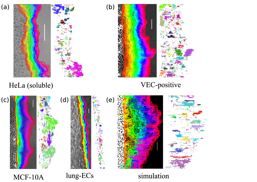
Figure 1: Cell front dynamics displays activity bursts. Examples of cell fronts and their time evolution and the corresponding activity maps. Cell fronts are colored according to time. Regions marked by the same color in the activity map move collectively. The scale bars are 100$\mu$m. a) HeLa cells moving on soluble collagen substrates. b) Mouse endothelial cells derived from embryonic stem cells (VEC-positive). c) Human mammary epithelial cells (MCF-10A). d) Mouse endothelial cells extracted from lungs (lung-ECs). e) Numerical simulations of the model.

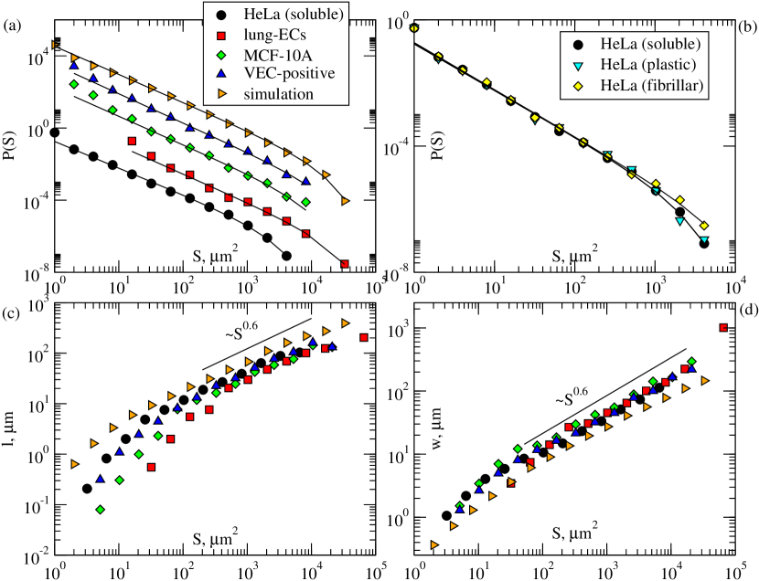
Figure 2: Cell activity bursts statistics displays scaling a) Distributions of the areas of activity clusters display power law scaling with a cutoff. The distributions for different cell types have been shifted for clarity. The slope obtained fitting the distributions is very similar for all cell types. b) Distributions of the areas of activity clusters for HeLa cells moving on different substrates. The scaling exponent is the same but the cutoff size for fibrillar collagen substrates is larger than for plastic and soluble collagen substrates. c) The average cluster length and d) the average cluster width scale with the cluster size with an exponent that is independent on the cell type.

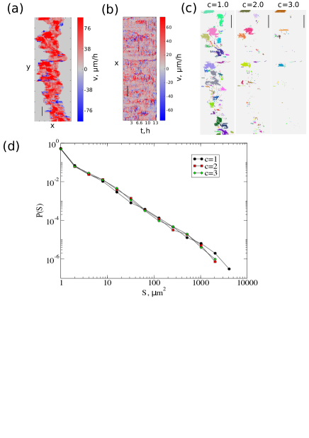
Figure S1: Determination of activity areas from images. Scale bars are 100$\mu$m. a) Spatial front velocity maps. Each pixel is colored according to the velocity of the front once it passes through that location. b) Spatio-temporal velocity map. Each pixel corresponds to the velocity ($v_{f}(x,t)$) at time $t$ of the front at point $x$ c) Activity clusters are obtained by setting threshold $c$ to the data in panel a. Results obtained with different values of $c$ are reported in three panels. d) Cluster size distributions for different values of $c$.

We perform migration experiments on different cell lines as described in the Materials and Methods section. We extract and record the cell front position as a function of time as shown in Fig. 1 for experiments (see Videos S1-S7) and in simulations (Video S8). The fronts show a rough structure with localized bursts of activity that is reminiscent of elastic lines moving in a pinning landscape [19, 20, 21, 22]. Spatio-temporal velocity fluctuations in moving fronts can be effectively quantified by constructing activity maps, as done previously for moving crack fronts [20] and fluid imbibition through porous media [21]. As discussed in the Materials and Methods section, from each time-lapse movie we construct a spatial map $v^{f}(x,y)$ measuring the velocity of the front at position $(x,y)$ (see Fig. S1). Using these maps we can define regions of coordinated activity by introducing a threshold $c$ for the velocity. The maps reported in Fig. 1 vividly illustrate the formation of localized clusters of activity similar to those found in fracture [20] and imbibition [21]. The corresponding distributions of cluster areas are reported in Fig. 2a for experiments on different cell types and for simulations. They all display a power law decay $P(S)\sim S^{-\tau}$ up to a cutoff length $S^{*}$.

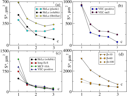
Figure S2: The characteristic cluster size $S^{*}=2\langle S^{2}\rangle/\langle S\rangle$ as a function of the velocity threshold $c$. a) Hela Cells on different substrates. b) Mouse endothelial cells expressing VE-cadherin or not. c) Comparison between different cell lines d) Simulations of the model for different values of $\beta$.

The exponent $\tau$ of the power law distribution appears to be similar for different cell types: the fitted values (see Table S1) are all similar within error bars ($\tau\simeq 1.4-1.6$) and remarkably close to the values recorded in crack front propagation [20]. As observed in moving cracks fronts, the cluster distributions, and in particular the cutoff to the power law decay, depends on the threshold $c$ used to identify the activity (see Materials and Methods and Fig. S1).The value of the cutoff $S^{*}$ is in all cases much larger than the typical size of a cell indicating that correlated activity spans multiple cells (Fig. S2). We also provide additional evidence for universality by measuring the relation between width, length and size of clusters Fig. 2cd. Also in this case, we find robust scaling across different cell lines and experimental conditions.

Cell migration on collagen matrix

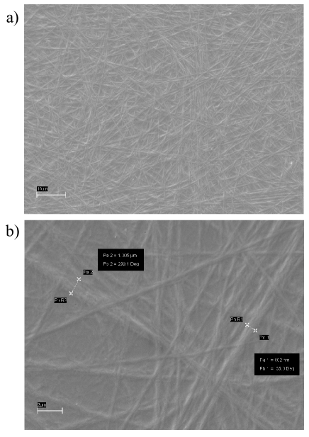
Figure S3: Scanning electron micrograph of the fibrillar collagen substrate at two different magnifications. From the high magnification image b) it is possible to estimate the fiber diameter.

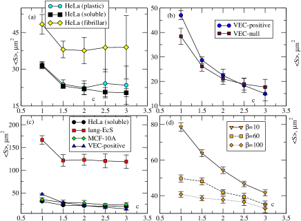
Figure S4: The average cluster size as a function of the velocity threshold $c$. a) HeLa Cells on different substrates. b) Mouse endothelial cells expressing VE-cadherin or not. c) Comparison between different cell lines d) Simulations of the model for different values of $\beta$.

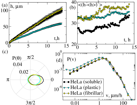
Figure S5: Dependence of the front dynamics on the substrate properties. a) Front position as a function of time indicates that fronts move slowly on plastic substrates. b) The standard deviation of the front (i.e. the front roughness) is larger for cells moving on fibrillar collagen. c) Angular velocity distribution as obtained from PIV. d) Distribution of absolute values of velocities as obtained by PIV.

To study quantitatively the effect of the substrate on the migration capability of cancer cells, we study wound healing under three different cell coating conditions: plastic (i. e. no coating), bovine soluble and fibrillar collagen. The two types of collagen substrates are exactly the same in terms of biochemistry, but differ in the structural organization. In Fig. S3, we show the fibrillar organization of our collagen substrate by scanning electron microscopy (SEM), while soluble collagen substrates display no fibrils or structure. As shown in Fig. 2b, the exponent of the activity cluster distribution is independent on the substrate. The average cluster size, however, is larger for fibrillar collagen than for soluble collagen and plastic, independently on the value of $c$ (see Fig 2b and Fig. S4a) To further quantify the role of the substrate in front propagation, we record average position of front as a function of time. As shown Fig. S5a, cell front motion is significantly slower on plastic substrates than on collagen ones. There is no noticeable difference in the average velocity of fronts moving on soluble and fibrillar collagen substrates. Fluctuations do, however, differ as shown by the standard deviation of the front position that is larger for cells moving on fibrillar collagen substrates (Fig S5b)

Velocity distributions

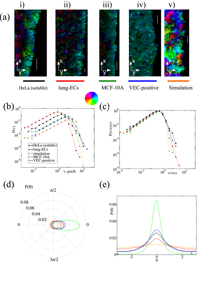
Figure 3: Cell velocity distributions display universal statistics a) Velocity maps for different cell types and for simulations as obtained from PIV. The colors indicate the orientation of the velocity following the color wheel. The length of the arrows is proportional to the magnitude of the velocity. The scale bars are 100$\mu$m. b) The corresponding distributions of velocity magnitudes. c) Scaling the velocities by their magnitude leads to a collapse of all the distributions, apart from small deviations in the tails. d,e) The distribution of the orientations of the velocities.

To better quantify the properties of the different experimental conditions, we resort to particle image velocimetry (PIV, see Materials and Methods) which allows to estimate local velocities treating the cell layer as a fluid. Representative examples of the local velocities for different cell types and for simulations are reported in Fig. 3a which displays the orientation of the velocity field (see also Videos S1-S7). While cells mostly advance towards the empty space there is significant motion also in the transverse and even in the opposite direction. This is summarized in the orientation distribution, revealing small differences due to cell types and substrates (Fig. 3de and S5c). Next, in Fig. 3b and S5d we report the distribution of the absolute value of the velocities extracted from PIV, indicating again quantitative differences between different cell types and substrates. Yet, the general shape of the velocity distribution is similar in all cases as shown in Fig. 3c where the velocities for each experiment are rescaled by their average value. This leads to a collapse of all the distributions, including the results of numerical simulations, apart from small deviations in the tails.

Effect of VE-cadherin knockdown

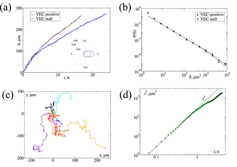
Figure 4: Knock down of VE-cadherin leads to faster fronts and individual cell motion. a) The time evolution of the front position for mouse endothelial cell expressing (VEC-positive) or not (VEC-null) VE-cadherin. VEC-null cells move faster. b) The corresponding cluster size distribution displays the same exponent and small changes in the cutoff. c) In the VEC null cases cells detach from the front and invade the space individually following trajectories as the ones illustrated. d) The average mean-square displacement of the trajectories indicates an initial ballistic regime followed by a slowing down.

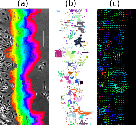
Figure S6: Front dynamics in mouse endothelial cells with VE-cadherin knock down (VEC-null). a) Fronts. b) Activity clusters. c) Results from PIV.

Internal couplings usually play a key role in avalanche statistics [25, 23, 26, 27]. To understand this point in our context, we assess the role of cell-cell interactions performing the same cell migration assay knocking down VE-cadherin in mouse endothelial cells [29]. VE-cadherin is an endothelial specific cadherin molecule located at adherent junctions which regulats adhesion between adjacent endothelial cells. Here we consider cells without VE-cadherin (VEC-null) but still expressing N-cadherin, another important molecule expressed by several types of cells such as neuronal, skeletal and heart muscle cells or fibroblasts [30]. Moreover, N-cadherin is highly expressed in mesenchymal stem cells and cancer cells that are highly invasive and poorly polarized [31]. As shown in Fig. 4a, VEC-null cell fronts move faster, but in a more disordered way (see Fig. S6), than VEC-positive fronts. The distribution of activity cluster areas is very similar in the two cases (Fig. 4a), with slightly larger cutoff size for VEC-positive cells (see Fig. S2). Despite these similarities, VEC-null cells tend to detach from the advancing front and move forward (see Video S9). We have tracked the trajectories of individual cells (Fig. 4c) and shown that they follow a persistent random walk, displaying ballistic motion at short time-scales (Fig. 4d). The combination of faster fronts and individual cells detachment confirms a more invasive phenotype for VEC-null cells [32].

Numerical simulations of an active particle model

In order to better understand how avalanche-like fluctuations arise in collective cell migration, we simulate the model of interacting active particle introduced in Ref. [10] (for the details see the Materials and Methods section). The geometry of the system, the size and number of particles are chosen to match the experimental images. Particles are first packed into a confined space and then allowed to invade space filled with “surface” particles. For the time scales considered in the present experiments, cell division is negligible and therefore we do not consider it in the model. The main tuning parameters of the model are the inter-particle velocity coupling $\beta$, the amplitude of the noise $\eta$ and the adhesion strength $U_{1}$. We also take into account the rough structure of the fibrillar collagen substrate by including a quenched (i.e. time independent) random force field with amplitude $\sigma_{\mathrm{r}f}$ and correlation length $\zeta$. Simulations representing plastic or soluble collagen substrate are performed without quenched disorder (i.e. $\sigma_{\mathrm{r}f}=0$), with fluctuations arising only from the random initial condition and the time-dependent noise in the dynamics. In addition to the random force field, the main difference between our simulations and Ref. [10] is that we do not consider leader cells.

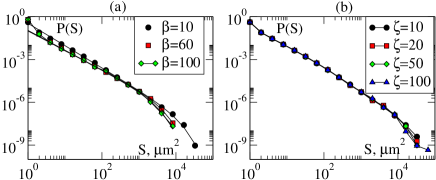
Figure S7: Simulated cluster size distributions a) for different $\beta$ (the strength of alignment between cells), b) for different $\zeta$ (correlation length of the random field).

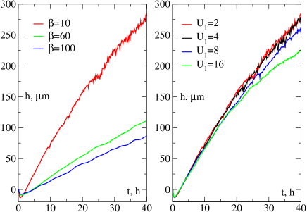
Figure S8: a) Simulations of the model for different values of $\beta$ show that fronts are slower when $\beta$ is increased. b) Simulations of the model for different values of the adhesion strength $U_{1}$ show that fronts are slower when $U_{1}$ is increased.

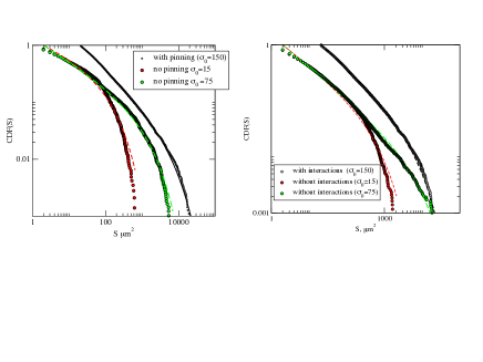
Figure S9: The non-binned cumulative distribution functions (CDF) of the cluster sizes from simulations a) with and without pinning (i. e. no surface particles and no random field) and b) with and without interactions (i.e. $\beta=0$, $U_{0}=U_{1}=0$). The lack of either pinning or interactions leads to clear deviation from a power law distribution, as also shown by fitting the simulation results with the maximum likelihood method. The fit yield scaling exponents $\tau=1.2$ (panel a, red), $\tau=1.38$ (panel a, green), $\tau=1.51$ (panel b, red), $\tau=1.56$ (panel b, green), but the fitted curves deviate systematically from the data and the scaling regime is extremely small. We also notice that in order to record a front at all in these conditions, one should also reduce the noise parameter $\sigma_{0}$.

The numerical simulations allow to reproduce with good accuracy all the salient features of collective cell migration revealed by our experiments as reported in Figs. 1-3. As already discussed, the numerical simulations reproduce the statistical features of activity bursts (Fig. 2) and cell velocities (Fig. 3). Furthermore, the numerical results illustrate the key role played by the substrate disorder, encoded in its correlation length $\zeta$, in determining the cutoff scale of the cluster size distribution (see Fig. S7). In particular, higher values of $\zeta$ correspond to larger activity clusters. This explains why cells move in larger activity bursts on fibrillar substrates, where disorder is stronger. Decreasing the velocity coupling $\beta$ or the adhesion strength $U_{1}$ increases the front velocity (Fig. S8) which should be compared with an analogous result observed when VE-cadherin is knocked down (Fig. 4). The model allows to explore the limits of universality. We observe an activity cluster distribution comparable to the experimentally measured one only for relatively small values of $\beta$. When $\beta$ is larger (e.g. $\beta=60$) the exponent $\tau$ is significantly smaller, suggesting the presence of different universality classes (see Fig. S7 and Table S2 for the results of the fits). Finally, we assess the relevance of interactions (i.e. performing simulations with $\beta=0$ and $U_{0}=U_{1}=0$) and pinning (i.e. no surface particles and no random field) and find that when either one of the two ingredients is missing the distribution is not a power law anymore (see Fig. S9). When neither pinning and interactions are present, we can not record a well defined front.

Universal scaling

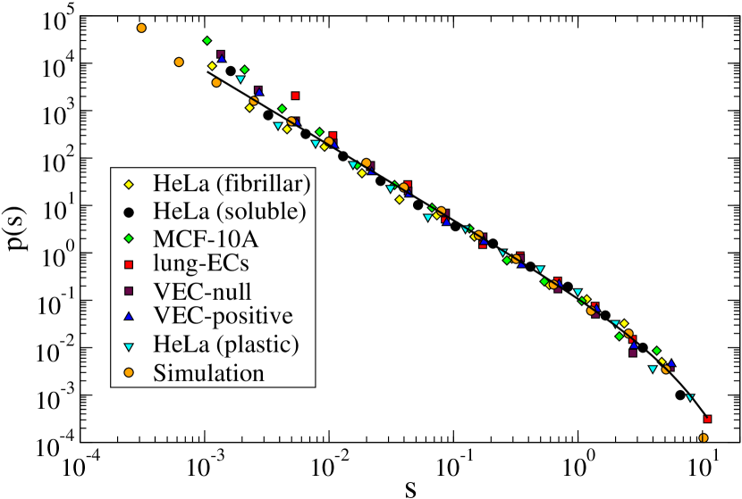
Figure 5: The distribution of activity clusters is universal. The distributions of the areas of activity clusters from Figs. 2 and 4 can all be collapsed into a single universal scaling function $p(s)=s^{-\tau}\exp(-Cs)$ (line) when plotted in terms of the reduced variable $s=S/S^{*}$.

The combinations of experimental results and numerical simulations suggests that the activity bursts observed in collective cell migration could be described by universal scaling laws as in non-equilibrium critical phenomena. In order to strengthen this conclusion it is, however, imperative to overcome the limitations of power law fitting [33] and focus instead on scaling functions, as indicated by Sethna et al. [28]. Ref. [27, 24] shows that in proximity of a depinning critical point, avalanche distributions $P(S)$ can be written as $P(S)=\frac{\langle S\rangle}{S^{*}}p(S/S^{*})$, where $S^{*}=\frac{\langle S^{2}\rangle}{2\langle S\rangle}$ and $p(s)$ is a universal scaling function. Here, we follow the same approach with our data and show that indeed all the experimental distributions, involving different cell lines and substrate, and those obtained from numerical simulations collapse into a single universal scaling curve as shown in Fig. 5. We thus perform a joint fit of all the distributions with a single scaling function $p(s)=s^{-\tau}\exp(-Cs)$, yielding $\tau=1.58\pm 0.02$ as best fitting parameter. This result provides a strong test of the universality of the bursty behavior we observe in collective cell migration.

Discussion

The collective motion of a cell layer as it invades an empty region has been extensively studied experimentally [7, 8, 9, 10] but the relation with the glassy features observed in confluent layers [34, 35] was not explored. The externally driven motion of disordered and glassy systems typically involves intermittent behavior and avalanches [28]. Our work shows that collective bursts of activity are also present in active matter with cells advancing in avalanches of widely distributed sizes. Similar intermittent activity [36] and scaling behavior has been previously recorded in animal [37] and even human mobility patterns [38] and it is thus intriguing to realize that it exists even at the cellular level. Finally, migration is a key property of tumor cells for tissue invasion and metastasis. Our detailed statistical analysis shows quantitatively how the organization and structure of the substrate, either gel or fibrillar, affects the way cells move. The final invasion velocity is the same but the motion is different, with larger intermittent fluctuations present on fibrillar substrates. This finding is interesting since it implies that cancer cells use different internal mechanisms to migrate depending on the environment, a fact that should be relevant for the metastatic process.

Materials and Methods

Collagen coating

Collagen substrates are prepared from a 3% solution of soluble bovine collagen in 0.01 HCl (code C4243, Sigma), kept in ice until use. Both solubilized (”soluble collagen”) and re-fibrillated collagen (”fibrillar collagen”) are prepared in 35 mm Petri dishes. For soluble substrates a sufficient amount of collagen solution is added to a Petri dish so that the bottom is covered, the excess is removed after 15 minutes and the dish is dried at room temperature for at least 2 hours. For fibrillar substrates, a mixture of 3% collagen solution (Code C4243, Sigma), 0.1N NaOH, 10% PBS (8:1:1) is prepared and 0.8mL are pipetted to the petri dish and incubated at 37^∘ C overnight to allow the proper gelification/refibrillation. After polymerization, samples are 5-10 micrometers in height.

Cell culture

HeLa cell line (ATCC CCL-2) is cultured in DMEM medium supplemented with 10% fetal calf serum, 2 mM L-glutamine, 100 U/ml penicillin, 100 mg/ml streptomycin and 0,25 mg/ml amphotericin B (Invitrogen, Milan, Italy) at 37^∘C and humidity (95% relative humidity), and CO2 concentration (5%). Cells are seeded in bovine soluble collagen, or fibrillar bovine collagen or without collagen-coated dishes and growth up to reach confluence overnight. Endothelial cells derived from embryonic stem cells with homozygous null mutation of the VE-cadherin gene (VEC null) [39]. The wild type form of VE-cadherin was introduced in these cells (VEC positive) as described in detail in [40] Endothelial cells isolated from lungs of wild type adult mice and cultured as previously described [29]. Starving medium was MCDB 131 (Invitrogen) with 1% BSA (EuroClone), 2-mM glutamine, 100 U/liter penicillin/streptomycin, and 1-mM sodium pyruvate. The MCF-10A cell line is a non-tumorigenic human mammary epithelial cell line (ATCC CRL10317) grown in DMEM/F12 supplemented with 5%horse serum, 20ng/ml EGF, 0.5mg/ml Hydrocortisone, 100ng/ml Choilera toxin, 10$\mu$g/ml Insulin.

Migration assay

For the migration assay, a wound is introduced in the central area of the confluent cell sheet by using a pipette tip and the migration followed by time-lapse imaging. Hela cells were stained with 10 $\mu$M Cell tracker green CMFDA (Molecular Probes) in serum-free medium for 30 minutes and then the complete medium was replaced. Mouse endothelial cell monolayers were wounded after an overnight starving, washed with PBS, and incubated at 37^∘C in starving medium. MCF-10A cell monolayers were wounded after an O/N doxycicline induction, washed with PBS, and incubated at 37^∘C in fresh media+doxycicline.

Time lapse imaging

For Hela cells, time-lapse multifield experiments were performed using an automated inverted Zeiss Axiovert S100 TV2 microscope (Carl Zeiss Microimaging Inc., Thornwood, NY) with a chilled Hamamatsu CCD camera OrcaII-ER. Displacements of the sample and the image acquisition are computer-controlled using Oko-Vision software (from Oko-lab). This Microscope was equipped with a cage incubator designed to maintain all the required environmental conditions for cell culture all around the microscopy workstation, thus enabling to carry out prolonged observations on biological specimens. Cell Tracker and Phase contrast images were acquired with an A-Plan 10x (NA 0.25) objective; the typical delay between two successive images of the same field was set to 10 minutes for 12 hours. For mouse endothelial cells and MCF-10A cells, time-lapse imaging of cell migration was performed on an inverted microscope (Eclipse TE2000-E; Nikon) equipped with an incubation chamber (OKOLab) maintained at 37^∘C in an atmosphere of 5% CO2. Movies were acquired with a Cascade II 512 (Photometrics) charge-coupled device (CCD) camera controlled by MetaMorph Software (Universal Imaging) using a 4X or 10× magnification objective lens (Plan Fluor 10×, NA 0.30). Images were acquired every 2 or 5 min over a 24h period. See Table S3 for the time lapse parameters.

Scanning Electron Microscopy

Collagen substrates are fixed with 2% glutaraldehyde in 0.1 M cacodylate buffer for 2 h at 4°C and post-fixed with 1% osmium tetroxyde in 0.1 M sodium cacodylate buffer (2 h, room temperature). After several washings with dH2O, they are dehydrated in an increasing ethanol scale and treated with a series of solutions of HMDS (Hexamethyldisilazane) and ethanol in different proportions (1:3, 1:1, 3:1 and 100% HMDS), mounted on stubs, covered with pure gold (Agar SEM Auto Sputter, Stansted, UK). The samples are observed under a scanning electron microscope(SEM) (LEO-1430, Zeiss, Oberkochen, Germany).

Particle image velocimetry (PIV)

The measurements of the velocity field were done using PIVlab app for Matlab [41, 42]. The method is based on the comparison of the intensity fields of two consequent photographs of cells. The difference in the intensity is converted into velocity field measured in $px/frame$. Then the velocity is converted to $\mu m/h$ through coefficient that is specific for each experiment, shown in table S3.

Border progression measurement

The method of border detection is based on the procedures described in  [43, 44]. The method is based on the border extraction procedure described in the manual of the Matlab software package (CellSegmentationExample).

Front activity maps

We analyze the propagation of the cell front, by measuring for each recorded image, and thus, at each time step $t$, the cell front position $y=h(x,t)$, along the abscissa $x$. We then construct a local velocity map of such interface $v^{f}(x,y)$, by computing the velocity of the cell front at each position of the front ($x$, $y=h(x,t)$) during its progression:

$$v^{f}(x,y=h(x,t_{i}))=\frac{h(x,t_{i+1})-h(x,t_{i})}{t_{i+1}-t_{i}}$$

Figure S1a provides such spatial color scale map $v^{f}(x,h(x,t))$ of the local velocity fluctuations for a typical wound healing experiment using HeLa cells moving on a soluble collagen substrate. The various regions of different color levels reveal an intermittent burst-like dynamics on a broad range of length scales. Such a complex dynamics can also be unveiled by representing the spatio-temporal map $v^{f}(x,t)$ giving the instantaneous velocity of each point of the cell front during its propagation, as shown in Fig. S1b. Occasional overhangs in the front are eliminated by the maximum value of $h$ for a given $x$. When the front locally moves backwards, we average all the velocity values at that point. To define areas of correlated activity, we consider the spatial map of the local front velocities $v^{f}(x,h(x,t))$ and define avalanches as clusters of velocities larger than an arbitrary threshold [20, 21]: $v^{f}(x,h(x,t))\geq c\langle v^{f}\rangle$, where $\langle v^{f}\rangle$ is the mean front velocity during the experiment Fig. S1c. Cluster sizes $S$ are given by the area of the clusters, and their shape is characterized by their length $l$ (lateral extension along $x$) and their width $w$ (extension in the mean direction of propagation $y$). The cutoff of the cluster size distribution depends slightly on $c$, but its scaling exponent does not (Fig. S1d).

Simulations of the active particle model

We simulate collective cell migration using a modified version of the model introduced in Ref. [10]. Here we introduce a pinning field and we do not consider a leader cell.

The main equation of motion is given by

$$\frac{d\mathbf{v}_{i}}{dt}=-\alpha\mathbf{v}_{i}+\sum_{j}\left[\frac{\beta}{N_{i}}(\mathbf{v}_{j}-\mathbf{v}_{i})+\mathbf{f}_{ij}\right]+\sigma(\rho_{i})\boldsymbol{\eta}_{i}+\mathbf{F}_{\mathrm{rf}}(\boldsymbol{x}_{i})\,$$ (1)

where the sum is restricted to the nearest neighbors of $i$, $\alpha$ is a damping parameter, $\beta$ is the velocity coupling strength, $\mathbf{f}_{ij}=-\nabla_{i}U(r_{ij})$ is the force between neighboring cells where

$$U(r)=U_{0}\exp(-(r/a_{0})^{2})+U_{1}(r-a_{1})^{2}H(r-a_{1})\,.$$ (2)

Here $H(x)$ is the Heaviside function $H(x)=1$ for $x>0$ and $H(x)=0$ otherwise, $U_{1}$ is the adhesion and $U_{0}$ the repulsive strength. The noise term $\sigma(\rho_{i})\boldsymbol{\eta}_{i}$, here $\boldsymbol{\eta}_{i}$ is an Ornstein-Uhlenbeck process with correlation time $\tau$:

$$\tau\frac{d\boldsymbol{\eta}_{i}}{dt}=-\boldsymbol{\eta}_{i}+\boldsymbol{\xi}_{i},$$ (3)

$\boldsymbol{\xi}_{i}$ is a delta-correlated white noise, independent for each cell $\langle\boldsymbol{\xi}_{i}(t)\boldsymbol{\xi}_{j}(t^{\prime})\rangle=\delta_{ij}\delta(t-t^{\prime})$ The amplitude of the noise term $\sigma$ depends on the density of the neighboring particles $\rho_{i}$:

$$\sigma(\rho_{i})=\sigma_{0}+(\sigma_{1}-\sigma_{0})(1-\rho_{i}/\rho_{0}).$$ (4)

The neighbors of each particle are defined in the same way as Ref. [10] The neighborhood of a particle $i$ is split into $6$ equal sectors. The particle closest to the particle $i$ in each sector (but closer then interaction radius of $100$ $\mu m$) is chosen to be a neighbor. The local density is computed then as $\rho_{i}=1/[\pi(\langle d\rangle/2)^{2}]$, where $\langle d\rangle$ is the average distance between cell $i$ and its $6$ neighbors (for sectors without neighbors the distance is taken to be $100$ $\mu m$). To model heterogeneous substrates we include an additional random force field $\mathbf{F}_{\mathrm{rf}}(\mathbf{x}_{i})$. A pair of Gaussian distributed random numbers, representing the two components of the random force, are placed on a square grid of spacing $\zeta$, quantifying the correlation length of the disorder. The value of random force between grid points is obtained through bilinear interpolation.

As in the original model, the free surface is modeled by surface particles, that are hindering cells to enter the empty space. The interaction between a surface particle and a cell is modeled as

$$\mathbf{f}_{ij}^{s}=-\nabla_{i}U^{s}(r_{ij})\,,$$ (5)

where $U^{s}(r)$ is $U^{s}(r)=A_{s}\exp(-(r/a_{s})^{2})$. A scalar damage variable $q$ is associated with each surface particles and follows the equation

$$\nu\frac{dq_{i}}{dt}=\sum_{j:\mathbf{r_{j}}\in S_{i}}|\mathbf{f_{ij}^{s}}|\,.$$ (6)

The values of the parameters that were used for simulations match the ones used in Ref. [10]: number of particles $N=4000$, size of the box $2L\times L$, $L=1000$ $\mu\mathrm{m}$, $\alpha=1.42\mathrm{h}^{-1}$, $\beta$, varying, but the value used in most of simulations was $\beta=10$ $\mathrm{h}^{-1}$, $\tau=1.39$ $\mathrm{h}^{-1}$, $\sigma_{0}=150$ $\mu\mathrm{m}\mathrm{h}^{-3/2}$, $\sigma_{1}=300$ $\mu\mathrm{m}\mathrm{h}^{-3/2}$, $U_{0}=2400$ $\mu\mathrm{m}^{2}/\mathrm{h}^{2}$, $a_{0}=8$ $\mu\mathrm{m}$, $U_{1}=2\mathrm{h}^{-2}$, $a_{1}=35\mu\mathrm{m}$, $\rho_{0}=4.0\times 10^{-3}\mu\mathrm{m}^{-2}$. $r_{s}$ the radius of interaction between a cell and a surface particle, is chosen to be $r_{s}=50\mu\mathrm{m}$, $\nu=7\mathrm{h}^{-1}$, $A_{s}=2400\mu\mathrm{m}^{2}/\mathrm{h}^{2}$, $a_{s}=8$ $\mu\mathrm{m}$, the threshold value $q_{i}=\theta$ after reaching which the surface particle disappears is taken to be $\theta=30$ $\mu\mathrm{m}$. The values for the parameters of the random field are also varied. Contrary to Ref. [10], we do not introduce any leader cell.

Data fitting

We fit the distribution of cluster sizes using the least-square method for binned histograms and the maximum likelihood method (see Fig. S10, Tables S1, S2 and Supporting Information for more details).

Authors Contributions

OC, MN, SS analyzed the data. CAMLP, CG, LL, MA, MS, UF, CM, GS, EM performed the experiments. OC, MN performed numerical simulations. CAMLP designed the experiments. OC, MJA, SZ designed the model. CAMLP, SZ wrote the manuscript. CAMLP, MJA, SZ coordinated the project.

Supplementary information

Details about the fitting methods

We employ different strategies to obtain the best parameters describing the cluster size distributions in simulations and experiments. We first consider the log-spaced binned probability density functions and perform a lest-square fitting with the function

$$f(x)=Ax^{-\tau}\exp(-Cx)\,,$$ (7)

To obtain a reliable estimate of the cutoff, we first take the logarithm of the distribution and fit it with the logarithm of Eq. 7. The fitting is performed in python using the pyFitting function (https://github.com/gdurin/pyFitting) and the results are reported in table S1 and S2 for experiments and simulations, respectively.

The second strategy relies on the maximum-likelihood estimate. Given the set of measured cluster sizes $S_{i}$, we consider the log-likelihood function

$$\mathcal{L}=-\sum_{i}\log(f(S_{i}))),$$ (8)

where the function $f(x)$ is given by Eq. 7. The function $\mathcal{L}$ is maximized with respect to the parameters $A$, $\tau$ and $\alpha$. The results are again reported in table S1 and S2. A comparison of the fitted function and the data can be presented in a way that is independent on binning by plotting the cumulative distribution functions in Fig. S10. The theoretical function in this case is given by

$$CDF=\frac{\Gamma(1-\tau,Cx)}{\Gamma(1-\tau,Cx_{min})}\,$$ (9)

where $\Gamma(a,b)$ is the incomplete gamma function.

Finally, we collapse together all the experimental probability density function into a unique set. To this end, we first compute the characteristic cluster size $S^{*}=\frac{\langle S^{2}\rangle}{2\langle S\rangle}$ from each experimental data set. We then rescale the cluster sizes, defining a reduced size $s=S/S^{*}$ and a scaling function $p(s)=P(S)\frac{S^{*}}{\langle S\rangle}$. Notice that $p(s)$ is not a distribution, since its integral is not equal to one. Once data for different experiments are rescaled according to this prescription, they are joined into a single set which is fitted by the least-square method using the function reported in Eq. 7. The result yields $A=0.13\pm 0.01$, $\tau=1.58\pm 0.02$ and $C=0.20\pm 0.03$.

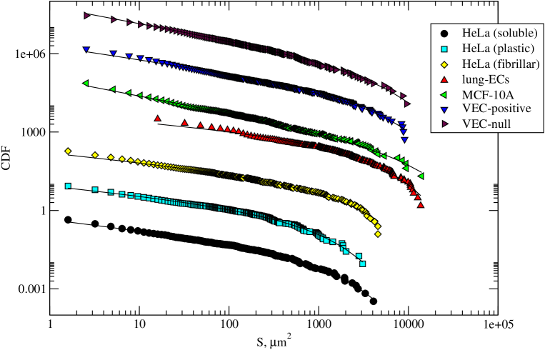
Figure S10: The non-binned cumulative distribution functions (CDF) of the cluster sizes for the different experiments are compared with the results of maximum likelihood estimates.

	Fitting			Maximum likelihood
Name	$A$	$\tau$	$C$	$\tau$	$C$	$x_{min}$
HeLa (soluble)	$0.18\pm 0.02$	$1.48\pm 0.03$	$0.00054\pm 5.2\times 10^{-5}$	$1.48\pm 0.10$	$(3.2\pm 2.43)\times 10^{-4}$	12.8
HeLa (plastic)	$0.17\pm 0.03$	$1.47\pm 0.05$	$0.0006\pm 0.0001$	$1.49\pm 0.09$	$(3.5\pm 2.8)\times 10^{-4}$	8.0
HeLa (fibrillar)	$0.19\pm 0.03$	$1.49\pm 0.04$	$(20\pm 7)\times 10^{-5}$	$1.34\pm 0.14$	$(2.82\pm 2.0)\times 10^{-4}$	28.8
lung-ECs	$0.81\pm 0.36$	$1.58\pm 0.07$	$(7.2\pm 1.4)\times 10^{-5}$	$1.45\pm 0.13$	$(1.1\pm 0.6)\times 10^{-4}$	176
MCF-10A	$0.17\pm 0.06$	$1.58\pm 0.08$	$(16.7\pm 9.2)\times 10^{-5}$	$1.56\pm 0.12$	$(1.2\pm 1.0)\times 10^{-4}$	43.5
VEC-positive	$0.33\pm 0.09$	$1.62\pm 0.05$	$(8.6\pm 4.9)\times 10^{-5}$	$1.55\pm 0.12$	$(1.2\pm 1.0)\times 10^{-4}$	53.8
VEC-null	$0.33\pm 0.04$	$1.62\pm 0.03$	$0.0001\pm 5\times 10^{-5}$	$1.61\pm 0.13$	$(1.7\pm 1.4)\times 10^{-4}$	46.1

Table S1: Best parameters obtained for the cluster distributions for experimental data by least-square fitting of the probability density function and by the maximum likelihood estimate. The smallest value of the cluster size ($x_{min}$) is also reported in the table.

	Fitting			Maximum likelihood
$\beta$	$A$	$\tau$	$C$	$\tau$	$C$	$x_{min}$
$10$	$0.34\pm 0.07$	$1.56\pm 0.04$	$(10\pm 1)\times 10^{-5}$	$1.60\pm 0.02$	$(6.3\pm 1.9)\times 10^{-4}$	$21$
$60$	$0.103\pm 0.007$	$1.37\pm 0.01$	$(3\pm 0.13)\times 10^{-4}$	$1.36\pm 0.05$	$(2.5\pm 0.8)\times 10^{-4}$	$16$
$100$	$0.11\pm 0.02$	$1.39\pm 0.04$	$(3.8\pm 0.3)\times 10^{-4}$	$1.33\pm 0.03$	$(3.9\pm 0.7)\times 10^{-4}$	$6$

Table S2: Best parameters obtained for the cluster distributions for simulated data by least-square fitting of the probability density function and by the maximum likelihood estimate. The smallest value of the cluster size ($x_{min}$) is also reported in the table.

Name	Number of fronts	1 px in $\mu$m	1 frame in min.
HeLa (plastic)	6	1.2658	10
HeLa (soluble)	5	1.2658	10
HeLa (fibrillar)	8	1.2658	10
lung-ECs	11	4	5
MCF-10A	8	1.6	5
VEC-positive	4	1.6	2
VEC-null	4	1.6	2

Table S3: Time-lapse parameters. We list the number of fronts analyzed for each case, The size of a pixel in each case and sizes and time step between two frames .

Supplementary video captions

• (Left) Time lapse of a representative sheet of Hela cells invading a fibrillar collagen substrate. The reconstructed front is reported in red. (Right) Evolution of the corresponding local velocity map obtained by PIV.

• (Left) Time lapse of a representative sheet of Hela cells invading a soluble collagen substrate. The reconstructed front is reported in red. (Right) Evolution of the corresponding local velocity map obtained by PIV.

• (Left) Time lapse of a representative sheet of Hela cells invading a plastic substrate. The reconstructed front is reported in red. (Right) Evolution of the corresponding local velocity map obtained by PIV.

• (Left) Time lapse of a representative sheet of lung derived endothelial cells. The reconstructed front is reported in red. (Right) Evolution of the corresponding local velocity map obtained by PIV.

• (Left) Time lapse of a representative sheet of MCF10-A cells invading a plastic substrate. The reconstructed front is reported in red. (Right) Evolution of the corresponding local velocity map obtained by PIV.

• (Left) Time lapse of a representative sheet of VEC-null mouse endothelial cells invading a plastic substrate. The reconstructed front is reported in red. (Right) Evolution of the corresponding local velocity map obtained by PIV.

• (Left) Time lapse of a representative sheet of VEC-positive mouse endothelial cells invading a plastic substrate. The reconstructed front is reported in red. (Right) Evolution of the corresponding local velocity map obtained by PIV.

• (Left) Representative simulation results. The reconstructed front is reported in red. (Right) Evolution of the corresponding local velocity map obtained by PIV.

• A representative trajectory (yellow) of an isolated VEC-null mouse endothelial cell.

References

- [1] Tambe DT, et al. (2011) Collective cell guidance by cooperative intercellular forces. Nat Mater 10:469–75.
- [2] Brugues A, et al. (2014) Forces driving epithelial wound healing. Nat Phys 10:683–690.
- [3] Haeger A, Krause M, Wolf K, Friedl P (2014) Cell jamming: collective invasion of mesenchymal tumor cells imposed by tissue confinement. Biochim Biophys Acta 1840:2386–95.
- [4] Lange JR, Fabry B (2013) Cell and tissue mechanics in cell migration. Exp Cell Res 319:2418–23.
- [5] Koch TM, Münster S, Bonakdar N, Butler JP, Fabry B (2012) 3d traction forces in cancer cell invasion. PLoS One 7:e33476.
- [6] Sacks MS, Sun W (2003) Multiaxial mechanical behavior of biological materials. Annu Rev Biomed Eng 5:251–84.
- [7] Vedula SRK, Ravasio A, Lim CT, Ladoux B (2013) Collective cell migration: a mechanistic perspective. Physiology (Bethesda) 28:370–9.
- [8] Szabó B, et al. (2006) Phase transition in the collective migration of tissue cells: Experiment and model. Phys Rev E 74:061908.
- [9] Poujade M, et al. (2007) Collective migration of an epithelial monolayer in response to a model wound. Proc Natl Acad Sci U S A 104:15988–93.
- [10] Sepúlveda N, et al. (2013) Collective cell motion in an epithelial sheet can be quantitatively described by a stochastic interacting particle model. PLoS Comput Biol 9:e1002944.
- [11] Haga H, Irahara C, Kobayashi R, Nakagaki T, Kawabata K (2005) Collective movement of epithelial cells on a collagen gel substrate. Biophys J 88:2250–6.
- [12] Ng MR, Besser A, Danuser G, Brugge JS (2012) Substrate stiffness regulates cadherin-dependent collective migration through myosin-ii contractility. J Cell Biol 199:545–63.
- [13] Saez A, Ghibaudo M, Buguin A, Silberzan P, Ladoux B (2007) Rigidity-driven growth and migration of epithelial cells on microstructured anisotropic substrates. Proc Natl Acad Sci U S A 104:8281–6.
- [14] Röttgermann PJF, Alberola AP, Rädler JO (2014) Cellular self-organization on micro-structured surfaces. Soft Matter 10:2397–404.
- [15] Oakes PW, et al. (2009) Neutrophil morphology and migration are affected by substrate elasticity. Blood 114:1387–95.
- [16] Metzner C, et al. (2015) Superstatistical analysis and modelling of heterogeneous random walks. Nat Commun 6:7516.
- [17] Serra-Picamal X, et al. (2012) Mechanical waves during tissue expansion. Nat Phys 8:628–634.
- [18] Banerjee S, Utuje KJC, Marchetti MC (2015) Propagating stress waves during epithelial expansion. Phys Rev Lett 114:228101.
- [19] Maloy KJ, Santucci S, Schmittbuhl J, Toussaint R (2006) Local waiting time fluctuations along a randomly pinned crack front. Phys Rev Lett 96:045501.
- [20] Tallakstad KT, Toussaint R, Santucci S, Schmittbuhl J, Maloy KJ (2011) Local dynamics of a randomly pinned crack front during creep and forced propagation: an experimental study. Phys Rev E Stat Nonlin Soft Matter Phys 83:046108.
- [21] Clotet X, Ortín J, Santucci S (2014) Disorder-induced capillary bursts control intermittency in slow imbibition. Phys Rev Lett 113:074501.
- [22] Durin G, Zapperi S (2000) Scaling exponents for Barkhausen avalanches in polycrystalline and amorphous ferromagnets. Phys Rev Lett 84:4075–4078.
- [23] Leschhorn H, Nattermann T, Stepanow S, Tang LH (1997) Driven interface depinning in a disordered medium. Ann Physik 6:1–34.
- [24] Rosso A, Le Doussal P, Wiese KJ (2009) Avalanche-size distribution at the depinning transition: A numerical test of the theory. Phys Rev B 80:144204.
- [25] Narayan O, Fisher DS (1992) Critical behavior of sliding charge-density waves in 4- epsilon dimensions. Phys Rev B 46:11520.
- [26] Chauve P, Doussal PL, Wiese KJ (2001) Renormalization of pinned elastic systems: how does it work beyond one loop. Phys Rev Lett 86:1785–1788.
- [27] Le Doussal P, Wiese KJ (2009) Size distributions of shocks and static avalanches from the functional renormalization group. Phys Rev E 79:051106.
- [28] Sethna J, Dahmen KA, Myers CR (2001) Crackling noise. Nature 410:242–244.
- [29] Giampietro C, et al. (2015) The actin-binding protein eps8 binds ve-cadherin and modulates yap localization and signaling. J Cell Biol 211:1177–92.
- [30] Goodwin M, Yap AS (2004) Classical cadherin adhesion molecules: coordinating cell adhesion, signaling and the cytoskeleton. J Mol Histol 35:839–44.
- [31] Wheelock MJ, Johnson KR (2003) Cadherins as modulators of cellular phenotype. Annu Rev Cell Dev Biol 19:207–35.
- [32] Giampietro C, et al. (2012) Overlapping and divergent signaling pathways of n-cadherin and ve-cadherin in endothelial cells. Blood 119:2159–70.
- [33] Clauset A, Shalizi CR, Newman ME (2009) Power-law distributions in empirical data. SIAM review 51:661–703.
- [34] Angelini TE, et al. (2011) Glass-like dynamics of collective cell migration. Proc Natl Acad Sci U S A 108:4714–9.
- [35] Park JA, et al. (2015) Unjamming and cell shape in the asthmatic airway epithelium. Nat Mater 14:1040–1048.
- [36] Weber CA, et al. (2015) Random bursts determine dynamics of active filaments. Proceedings of the National Academy of Sciences 112:10703–10707.
- [37] Ginelli F, et al. (2015) Intermittent collective dynamics emerge from conflicting imperatives in sheep herds. Proc Natl Acad Sci U S A 112:12729–34.
- [38] Song C, Koren T, Wang P, Barabasi AL (2010) Modelling the scaling properties of human mobility. Nat Phys 6:818–823.
- [39] Balconi G, Spagnuolo R, Dejana E (2000) Development of endothelial cell lines from embryonic stem cells: A tool for studying genetically manipulated endothelial cells in vitro. Arterioscler Thromb Vasc Biol 20:1443–51.
- [40] Lampugnani MG, et al. (2002) Ve-cadherin regulates endothelial actin activating rac and increasing membrane association of tiam. Mol Biol Cell 13:1175–89.
- [41] Thielicke W (2014) The flapping flight of birds: Analysis and application. Ph.D. thesis.
- [42] Thielicke W, Stamhuis E (2014) Pivlab – towards user-friendly, affordable and accurate digital particle image velocimetry in matlab 2.
- [43] Johnston ST, Simpson MJ, McElwain DLS (2014) How much information can be obtained from tracking the position of the leading edge in a scratch assay? Journal of The Royal Society Interface 11.
- [44] Treloar KK, Simpson MJ (2013) Sensitivity of edge detection methods for quantifying cell migration assays. PLoS One 8:e67389.