A Theoretical Analysis of Noisy Sparse Subspace Clustering on Dimensionality-Reduced Data

Abstract

Subspace clustering is the problem of partitioning unlabeled data points into a number of clusters so that data points within one cluster lie approximately on a low-dimensional linear subspace. In many practical scenarios, the dimensionality of data points to be clustered are compressed due to constraints of measurement, computation or privacy. In this paper, we study the theoretical properties of a popular subspace clustering algorithm named sparse subspace clustering (SSC) and establish formal success conditions of SSC on dimensionality-reduced data. Our analysis applies to the most general fully deterministic model where both underlying subspaces and data points within each subspace are deterministically positioned, and also a wide range of dimensionality reduction techniques (e.g., Gaussian random projection, uniform subsampling, sketching) that fall into a subspace embedding framework (Meng & Mahoney, 2013; Avron et al., 2014). Finally, we apply our analysis to a differentially private SSC algorithm and established both privacy and utility guarantees of the proposed method.

1 Introduction

Subspace clustering is an unsupervised learning paradigm aiming at grouping unlabeled data points into disjoint clusters so that data points within each cluster lie near a low-dimensional linear subspace. It has found many successful applications in computer vision and machine learning, as many high dimensional data can be approximated by a union of low-dimensional subspaces. Examples include motion trajectories (Costeira & Kanade, 1998), face images (Basri & Jacobs, 2003), network hop counts (Eriksson et al., 2012), movie ratings Zhang et al. (2012) and social graphs (Jalali et al., 2011).

The success in applications is made possible by two decades of algorithmic research on this problem. Popular approaches include Expectation-Maximization-style methods such as K-plane (Bradley & Mangasarian, 2000) and Q-flat (Tseng, 2000), algebraic methods such as generalized principal component analysis (Vidal et al., 2005), matrix factorization methods (Costeira & Kanade, 1998), bottom-up local affinity-based methods such as those proposed by Yan & Pollefeys (2006); Ma et al. (2007), and convex optimization based approaches including Low Rank Representation (LRR, Liu et al., 2013) and Sparse Subspace Clustering (SSC, Elhamifar & Vidal, 2013).

In this paper we consider the SSC algorithm, which has drawn much interest from the literature. It is known that SSC enjoys superb performance in practice (Elhamifar & Vidal, 2013) and has theoretical guarantees under fairly general conditions (Soltanolkotabi et al., 2012; Wang & Xu, 2013; Soltanolkotabi et al., 2014). Let $\mathbf{X}\in\mathbb{R}^{d\times N}$ denote the data matrix, where $d$ is the ambient dimension and $N$ is the number of data points. For noiseless data (i.e., data points lie exactly on low-rank subspaces), the exact SSC algorithm solves

$$\min_{\boldsymbol{c}_{i}\in\mathbb{R}^{N}}\|\boldsymbol{c}_{i}\|_{1},\quad\text{s.t. }\boldsymbol{x}_{i}=\mathbf{X}\boldsymbol{c}_{i},\boldsymbol{c}_{ii}=0.$$ (1.1)

for each data point $\boldsymbol{x}_{i}$ to obtain self regression solutions $\boldsymbol{c}_{i}\in\mathbb{R}^{N}$. For noisy data, the following Lasso version of SSC is often used in practice:

$$\min_{\boldsymbol{c}_{i}\in\mathbb{R}^{N}}\|\boldsymbol{x}_{i}-\mathbf{X}\boldsymbol{c}_{i}\|_{2}^{2}+2\lambda\|\boldsymbol{c}_{i}\|_{1},\quad\text{s.t. }\boldsymbol{c}_{ii}=0.$$ (1.2)

The intuition of SSC is to learn a sparse “self-representation” matrix $\mathbf{C}\in\mathbb{R}^{N\times N}$ over all data points by imposing an $\ell_{1}$ penalty on the representation coefficients. This can also be thought of as a convex optimization based graph embedding that captures a specific type of relationship among data points. Each non-zero entry of $\mathbf{C}$ is an edge connecting two data points. It has been shown in Soltanolkotabi et al. (2012); Wang & Xu (2013); Soltanolkotabi et al. (2014) that under mild conditions the learned representation/similarity matrix $\mathbf{C}$ contains no false connections, in that every such edge connects only data points that belong to the same cluster. Finally, spectral clustering (Ng et al., 2002) is performed on the learned similarity matrix $|\mathbf{C}|+|\mathbf{C}|^{T}$ to cluster the $N$ data points into disjoint clusters.

Although success conditions for both exact SSC and Lasso SSC have been extensively analyzed in previous literature, in practice it is inefficient or even infeasible to operate on data with high dimension. Some types of dimensionality reduction is usually required (Vidal, 2010). In this paper, we propose a theoretical framework that analyzes SSC under many popular dimensionality reduction settings, including

• Compressed measurement: With compressed measurement dimensionality-reduced data are obtained by multiplying the original data typically with a random Gaussian matrix. We show that SSC provably succeeds when the projected dimension is on the order of a low-degree polynomial of the maximum intrinsic rank of each subspace.

• Efficient computation: By using fast Johnson-Lindenstrauss transform (FJLT) (Ailon & Chazelle, 2009) or sketching (Charikar et al., 2004; Clarkson & Woodruff, 2013) one can reduce the data dimension for computational efficiency while still preserving important structures in the underlying data. We prove similar results for both FJLT and sketching.

• Handling missing data: In many applications, the data matrix may be incomplete due to measurement and sensing limits. It is shown in this paper that, when data meet some incoherent criteria, uniform feature sampling suffices for SSC.

• Data privacy: Privacy is an important concern in modern machine learning applications. It was shown that Gaussian random projection with added Gaussian noise preserves both information-theoretic (Zhou et al., 2009) and differential privacy (Kenthapadi et al., 2013). We provide a utility analysis which shows that SSC can achieve exact subspace detection despite stringent privacy constraints.

The main contribution of this paper is a unified framework for analyzing sparse subspace clustering on dimensionality-reduced data. In particular, we prove that a subspace embedding property (Clarkson & Woodruff, 2013; Avron et al., 2014) is sufficient to guarantee successful execution of the SSC algorithm after compression. Furthermore, the lowest dimension we can compress the data into only scales as a low-degree polynomial of the intrinsic dimension $r$ and does not depend (up to poly-logarithmic factors) on either the ambient dimension $d$ or the total number of data points $N$. This is a much desired property, because in practical subspace clustering applications both $d$ and $N$ are huge, while the intrinsic dimensionality $r$ typically stays at nearly a constant (Vidal, 2010; Wang & Xu, 2013). We also show by simple derivations and citing existing results that all of the above-mentioned data compression schemes (Gaussian projection, uniform subsampling, FJLT, sketching) are subspace embeddings, and hence fall into the perturbation analysis framework we formulated. Finally, as an application of our analysis, we propose a differentially private SSC algorithm by random projection followed by Gaussian perturbation and prove both privacy and utility guarantees of the proposed algorithm.

1.1 Problem setup and notations

Notations

For a vector $\boldsymbol{x}$, $\|\boldsymbol{x}\|_{p}=(\sum_{i}{|\boldsymbol{x}_{i}|^{p}})^{1/p}$ denotes the vector $p$-norm of $\boldsymbol{x}$. For a matrix $\mathbf{A}$, $\|\mathbf{A}\|_{p}=\sup_{\boldsymbol{x}\neq 0}\|\mathbf{A}\boldsymbol{x}\|_{p}/\|\boldsymbol{x}\|_{p}$ denotes the operator $p$-norm of $\mathbf{A}$. In particular, $\|\mathbf{A}\|_{2}=\sigma_{\max}(\mathbf{A})$ is the spectral norm of $\mathbf{A}$. The subscript $p$ is sometimes dropped for $p=2$; that is, $\|\boldsymbol{x}\|=\|\boldsymbol{x}\|_{2}$ and $\|\mathbf{A}\|=\|\mathbf{A}\|_{2}$.

The uncorrupted data matrix is denoted as $\mathbf{Y}\in\mathbb{R}^{d\times N}$, where $d$ is the ambient dimension and $N$ is the total number of data points. $\mathbf{Y}$ is normalized so that each column has unit two norm, which does not alter the union of subspaces on which $\mathbf{Y}$ lies. Each column in $\mathbf{Y}$ belongs to a union of $k$ subspaces $\mathcal{U}^{(1)}\cup\cdots\cup\mathcal{U}^{(k)}$. For each subspace $\mathcal{U}^{(\ell)}$ we write $\mathbf{Y}^{(\ell)}=(\boldsymbol{y}_{1}^{(\ell)},\cdots,\boldsymbol{y}_{N_{\ell}}^{(\ell)})$ for all columns belonging to $\mathcal{U}^{(\ell)}$, where $N_{\ell}$ is the number of data points in $\mathcal{U}^{(\ell)}$ and $\sum_{\ell=1}^{k}{N_{\ell}}=N$. We assume the rank of the $\ell$th subspace $\mathcal{U}^{(\ell)}$ is $r_{\ell}$ and define $r=\max_{\ell}{r_{\ell}}$. In addition, we use $\mathbf{U}^{(\ell)}\in\mathbb{R}^{d\times r_{\ell}}$ to represent an orthonormal basis of $\mathcal{U}^{(\ell)}$. The observed matrix is denoted by $\mathbf{X}\in\mathbb{R}^{d\times N}$. Under the noiseless setting we have $\mathbf{X}=\mathbf{Y}$; for the noisy setting we have $\mathbf{X}=\mathbf{Y}+\mathbf{Z}$ where $\mathbf{Z}\in\mathbb{R}^{d\times N}$ is a noise matrix which can be either deterministic or stochastic.

We use “$-i$” subscript to denote all except the $i$th column in a data matrix. For example, $\mathbf{Y}_{-i}=(\boldsymbol{y}_{1},\cdots,\boldsymbol{y}_{i-1},\boldsymbol{y}_{i+1},\cdots,\boldsymbol{y}_{N})$ and $\mathbf{Y}_{-i}^{(\ell)}=(\boldsymbol{y}_{1}^{(\ell)},\cdots,\boldsymbol{y}_{i-1}^{(\ell)},\boldsymbol{y}_{i+1}^{(\ell)},\cdots,\boldsymbol{y}_{N_{\ell}}^{(\ell)})$. For any matrix $\mathbf{A}$, let $\mathcal{Q}(\mathbf{A})=\mathrm{conv}(\pm\boldsymbol{a}_{1},\cdots,\pm\boldsymbol{a}_{N})$ denote the symmetric convex hull spanned by all columns in $\mathbf{A}$. For any subspace $\mathcal{U}$ and vector $\boldsymbol{v}$, denote $\mathcal{P}_{\mathcal{U}}\boldsymbol{v}=\mathrm{argmin}_{\boldsymbol{u}\in\mathcal{U}}{\|\boldsymbol{u}-\boldsymbol{v}\|_{2}}$ as the projection of $\boldsymbol{v}$ onto $\mathcal{U}$.

Models

We consider three models for the uncorrupted data $\mathbf{Y}$ of increasing strictness of assumptions. Such hierarchy of models were first introduced in Soltanolkotabi et al. (2012) and have served as reference models in existing analysis of SSC methods (Soltanolkotabi et al., 2014; Heckel & Bolcskei, 2013; Wang & Xu, 2013; Park et al., 2014):

• Fully deterministic model: in the fully deterministic model both the underlying low-rank subspaces $\mathcal{U}^{(1)},\cdots,\mathcal{U}^{(k)}$ and the data points $\boldsymbol{y}_{1}^{(\ell)},\cdots,\boldsymbol{y}_{N_{\ell}}^{(\ell)}$ in each subspace are deterministically placed. This is the most general model for subspace clustering (except the model-free agnostic settings considered in the projective clustering literature (Feldman et al., 2013)) as no stochastic or i.i.d. type assumptions are imposed on either the subspaces or the data points.

• Semi-random model: In the semi-random model the underlying subspaces $\mathcal{U}^{(1)},\cdots,\mathcal{U}^{(k)}$ are again deterministically placed; however, (uncorrupted) data points within each subspace are assumed to be sampled i.i.d. uniformly at random from the unit sphere of the corresponding low-dimensional subspace. One advantage of semi-random modeling is its interpretability: success conditions of SSC could be fully characterized using affinities between subspaces and number of data points per subspace (Soltanolkotabi et al., 2012, 2014; Wang & Xu, 2013).

• Fully-random model: In the fully random model both the underlying subspaces and data points within each subspace are sampled uniformly at random.

Apart from data models, we also consider two models when data $\mathbf{Y}$ are corrupted by noise $\mathbf{Z}=(\boldsymbol{z}_{1},\cdots,\boldsymbol{z}_{N})\neq\mathbf{0}$. In the deterministic noise model, each noise vector $\boldsymbol{z}_{i}$ is adversarially placed, except that the largest maximum magnitude $\max_{1\leq i\leq n}\|\boldsymbol{z}_{i}\|_{2}^{2}$ is upper bounded by a noise parameter $\xi$. In the stochastic noise model, $\boldsymbol{z}_{i}$ is assumed to be i.i.d. sampled from a zero-mean multivariate distribution $\mathcal{N}_{d}(\boldsymbol{0},\sigma^{2}/d\cdot\mathbf{I}_{d\times d})$ for some noise parameter $\sigma$. Note that here we divide the variance $\sigma^{2}$ by $d$ to keep the magnitude of noise constant and not increasing with number of dimensions. In our analysis, the stochastic noise model allows for larger magnitude of noise compared to the deterministic (adversarial) noise setting as it places stronger assumptions on the properties of the noise.

Methods

The first step is to perform dimensionality reduction on the observation matrix $\mathbf{X}$. More specifically, for a target projection dimension $p<d$, the projected observation matrix $\widetilde{\mathbf{X}}^{\prime}\in\mathbb{R}^{p\times N}$ is obtained by first computing $\widetilde{\mathbf{X}}=\mathbf{\Psi}\mathbf{X}$ for some random projection matrix $\mathbf{\Psi}\in\mathbb{R}^{p\times d}$ and then normalizing it so that each column in $\widetilde{\mathbf{X}}^{\prime}$ has unit two norm. Afterwards, Lasso self-regression as formulated in Eq. (1.2) is performed for each column in $\widetilde{\mathbf{X}}^{\prime}$ to obtain the similarity matrix $\mathbf{C}=\{\boldsymbol{c}_{i}\}_{i=1}^{N}\in\mathbb{R}^{N\times N}$. Spectral clustering is then be applied to $\mathbf{C}$ to obtain an explicit clustering of $\mathbf{X}$. In this paper we use the normalized-cut algorithm Shi & Malik (2000) for spectral clustering.

Evaluation measures

To evaluate the quality of obtained similarity matrix $\mathbf{C}$, we consider the Lasso subspace detection property defined in Wang & Xu (2013). More specifically, $\mathbf{C}$ satisfies Subspace Detection Property (SDP) if for each $i\in\{1,\cdots,N\}$ the following holds: 1) $\boldsymbol{c}_{i}$ is a non-trivial solution. That is, $\boldsymbol{c}_{i}$ is not the zero vector; 2) if $c_{ij}\neq 0$ then data points $\boldsymbol{x}_{i}$ and $\boldsymbol{x}_{j}$ belong to the same subspace cluster. The second condition alone is referred to as “Self-Expressiveness Property” (SEP) in Elhamifar & Vidal (2013). Note that we do not require $c_{ij}\neq 0$ for every pair of $\boldsymbol{x}_{i},\boldsymbol{x}_{j}$ belonging to the same cluster. We also remark that in general SEP is not necessary for spectral clustering to succeed, cf. Wang & Xu (2013) .

1.2 Related Work

Heckel et al. (2014) analyzed SSC and threshold-based subspace clustering (TSC, Heckel & Bolcskei, 2013) on dimension-reduced noiseless data. Heckel et al. (2015), which was arxived concurrently with the earlier version in ICML of our paper, further generalized Heckel et al. (2014), with analysis of TSC and SSC-OMP on noisy data. One important limitation of both Heckel et al. (2014, 2015) is that the data points in each subspace is assumed to be drawn uniformly at random, corresponding to the semi-random model specified in Sec. 1.1. Though amenable for theoretical analysis, the semi-random model deviates significantly from subspace clustering practice because data points, even on the same subspace, are not distributed uniformly at random. This is particularly true when data lies on affine subspaces and the “homogeneous embedding” trick is used, which is almost always the case in practice (Elhamifar & Vidal, 2013). The added dimension in homogeneous embedding is constant valued and breaks any semi-random assumptions. In this paper, we complement the results of Heckel et al. (2015) by analyzing noisy SSC under the fully deterministic model, where no stochastic assumptions imposed upon the data points. Our analysis naturally leads to interpretable noise conditions under the semi-random model.

Our proof technique also significantly differs from the one in Heckel et al. (2015) which focused primarily on perturbation of subspace affinities (Soltanolkotabi et al., 2012). When data points are not uniformly distributed, subspace affinity as defined by Soltanolkotabi et al. (2012); Heckel et al. (2015) no longer serves as a good characterization of the difficulty of the subspace clustering problem. Instead, we propose novel perturbation analysis of the dual solution of the noisy SSC formulation, which is applicable under the fully deterministic setting. Finally, we remark that an earlier conference version of this paper (Wang et al., 2015a) which summarized most parts of the deterministic analysis in this paper (including analysis for noisy data) was published before Heckel et al. (2015). Another difference, as noted in Heckel et al. (2015), is that in our analysis the projected noise is added after normalization of the projected signal. We consider this to be a minor difference because the length of the projected signal is close to the length of the original signal, thanks to Proposition 2.7. In particular, for semi-random or fully-random models the length of each data point is very close to one with high probability, and hence the noisy model we analyzed behaves similarly to the one considered in Heckel et al. (2015).

Arpit et al. proposed a novel dimensionality reduction algorithm to preserve independent subspace structures Arpit et al. (2014). They showed that by using $p=2k$, where $k$ is the number of subspaces, one can preserve the independence structure among subspaces. However, their analysis only applies to noiseless and independent subspaces, while our analysis applies even when the least principal angle between two subspaces diminishes and can tolerate a fair amount of noise. Furthermore, in our analysis the target dimension $p$ required depends on the maximum intrinsic subspace dimension $r$ instead of $k$. Usually $r$ is quite small in practice (Elhamifar & Vidal, 2013; Basri & Jacobs, 2003).

Another relevant line of research is high-rank matrix completion. In Eriksson et al. (2012) the authors proposed a neighborhood selection based algorithm to solve multiple matrix completion problems. However, Eriksson et al. (2012) requires an exponential number of data points to effectively recover the underlying subspaces. In contrast, in our analysis $N$ only needs to scale polynomially with $r$. In addition, strong distributional assumptions are imposed in Eriksson et al. (2012) to ensure that data points within the same subspace lie close to each other, while our analysis is applicable to the fully general deterministic setting where no such distributional properties are required.

2 Dimension reduction methods

In this section we review several popular dimensionality reduction methods and show that they are subspace embeddings. To keep the presentation simple, proofs of results in this section are presented in Appendix A. A linear projection $\mathbf{\Psi}\in\mathbb{R}^{p\times d}$ is said to be a subspace embedding if for some $r$-dimensional subspace $\mathcal{L}\subseteq\mathbb{R}^{d}$ the following holds:

$$\Pr_{\mathbf{\Psi}}\left[\|\mathbf{\Psi}\boldsymbol{x}\|\in(1\pm\epsilon)\|\boldsymbol{x}\|,\forall\boldsymbol{x}\in\mathcal{L}\right]\geq 1-\delta.$$ (2.1)

The following proposition is a simple property of subspace embeddings.

Proposition 2.1.

Fix $\epsilon,\delta>0$. Suppose $\mathbf{\Psi}$ is a subspace embedding with respect to a union of subspaces $\mathcal{B}=\{\mathrm{span}(\mathcal{U}^{(\ell)}\cup\mathcal{U}^{(\ell^{\prime})});\ell,\ell^{\prime}\in[k]\}\cup\{\boldsymbol{x}_{i},\boldsymbol{z}_{i};i\in[N]\}$ with parameters $r^{\prime}=2r$, $\epsilon^{\prime}=\epsilon/3$ and $\delta^{\prime}=2\log((k+N)/\delta)$. Then with probability $\geq 1-\delta$ for all $\boldsymbol{x},\boldsymbol{y}\in\mathcal{U}^{(\ell)}\cup\mathcal{U}^{(\ell^{\prime})}$ we have

$$\big{|}\langle\boldsymbol{x},\boldsymbol{y}\rangle-\langle\mathbf{\Psi}\boldsymbol{x},\mathbf{\Psi}\boldsymbol{y}\rangle\big{|}\leq\epsilon\left(\frac{\|\boldsymbol{x}\|^{2}+\|\boldsymbol{y}\|^{2}}{2}\right);$$ (2.2)

furthermore, for all $\boldsymbol{x}\in\{\boldsymbol{x}_{1},\boldsymbol{z}_{1},\cdots,\boldsymbol{x}_{N},\boldsymbol{z}_{N}\}$ the following holds:

$$(1-\epsilon)\|\boldsymbol{x}\|_{2}^{2}\leq\|\mathbf{\Psi}\boldsymbol{x}\|_{2}^{2}\leq(1+\epsilon)\|\boldsymbol{x}\|_{2}^{2}.$$ (2.3)

Random Gaussian projection

In a random Gaussian projection matrix $\mathbf{\Psi}$ each entry $\mathbf{\Psi}_{ij}$ is generated from i.i.d. Gaussian distributions $\mathcal{N}(0,1/\sqrt{p})$, where $p$ is the target dimension after projection. Using standard Gaussian tail bounds and Johnson-Lindenstrauss argument we get the following proposition.

Proposition 2.2.

Gaussian random matrices $\mathbf{\Psi}\in\mathbb{R}^{p\times d}$ is a subspace embedding with respect to $\mathcal{B}$ if

$$p\geq 2\epsilon^{-2}(r+\log(2k^{2}/\delta)+\sqrt{4r\log(2k^{2}/\delta)}+12\log(4N/\delta)).$$ (2.4)

Uniform row sampling

For uniform row sampling each row in the observed data matrix $\mathbf{X}$ is sampled independently at random so that the resulting matrix has $p$ non-zero rows. Formally speaking, each row of the projection matrix $\mathbf{\Omega}$ is sampled i.i.d. from the distribution $\Pr\left[\boldsymbol{\Omega}_{i\cdot}=\sqrt{\frac{d}{p}}\boldsymbol{e}_{j}\right]=\frac{1}{d}$, where $i\in[p]$, $j\in[d]$ and $\boldsymbol{e}_{j}$ is a $d$-dimensional indicator vector with only the $j$th entry not zero.

For uniform row sampling to work, both the observation matrix $\mathbf{X}$ and the column space of the uncorrupted data matrix $\mathbf{Y}$ should satisfy certain incoherence conditions. In this paper, we apply the following two types of incoherence/spikiness definitions, which are widely used in the low rank matrix completion literature Recht (2011); Balzano et al. (2010); Krishnamurthy & Singh (2014).

Definition 2.1 (Column space incoherence).

Suppose $\mathcal{U}$ is the column space of some matrix and $\mathrm{rank}(\mathcal{U})=r$. Let $\mathbf{U}\in\mathbb{R}^{d\times r}$ be an orthonormal basis of $\mathcal{U}$. The incoherence of $\mathcal{U}$ is defined as

$$\mu(\mathcal{U}):=\frac{d}{r}\max_{i=1,\cdots,d}{\|\mathbf{U}_{(i)}\|_{2}^{2}},$$ (2.5)

where $\mathbf{U}_{(i)}$ indicates the $i$th row of $\mathbf{U}$.

Definition 2.2 (Column spikiness).

For a vector $\boldsymbol{x}\in\mathbb{R}^{d}$, the spikiness of $\boldsymbol{x}$ is defined as

$$\mu(\boldsymbol{x}):=d\|\boldsymbol{x}\|_{\infty}^{2}/\|\boldsymbol{x}\|_{2}^{2},$$ (2.6)

where $\|\boldsymbol{x}\|_{\infty}=\max_{i}{|x_{i}|}$ denotes the vector infinite norm.

Under these two conditions, uniform row sampling operator $\mathbf{\Omega}$ is a subspace embedding.

Proposition 2.3.

Suppose $\max_{\ell=1}^{k}{\mu(\mathcal{U}^{(\ell)})}\leq\mu_{0}$ and $\max_{i=1}^{N}{\max(\mu(\boldsymbol{x}_{i}),\mu(\boldsymbol{z}_{i}))}\leq\mu_{0}$ for some constant $\mu_{0}>0$. The uniform sampling operator $\mathbf{\Omega}$ is a subspace embedding with respect to $\mathcal{B}$ if

$$p\geq 8\epsilon^{-2}\mu_{0}(r\log(4rk^{2}/\delta)+\log(8N/\delta)).$$ (2.7)

FJLT and sketching

The Fast Johnson-Lindenstrauss Transform (FJLT, Ailon & Chazelle, 2009) computes a compressed version of a data matrix $\mathbf{X}\in\mathbb{R}^{d\times N}$ using $O(d\log d+p)$ operations instead of $O(pd)$ per column with high probability. The projection matrix $\mathbf{\Phi}$ can be written as $\mathbf{\Phi}=\mathbf{P}\mathbf{H}\mathbf{D}$, where $\mathbf{P}\in\mathbb{R}^{p\times d}$ is a sparse JL matrix, $\mathbf{H}\in\mathbb{R}^{d\times d}$ is a deterministic Walsh-Hadamard matrix and $\mathbf{D}\in\mathbb{R}^{d\times d}$ is a random diagonal matrix. Details of FJLT can be found in Ailon & Chazelle (2009).

Sketching (Charikar et al., 2004; Clarkson & Woodruff, 2013) is another powerful tool for dimensionality reduction on sparse inputs. The sketching operator $\mathbf{S}:\mathbb{R}^{d}\to\mathbb{R}^{p}$ is constructed as $\mathbf{S}=\mathbf{\Pi}\mathbf{\Sigma}$, where $\mathbf{\Pi}$ is a random permutation matrix and $\mathbf{\Sigma}$ is a random sign diagonal matrix. The projected vector $\mathbf{S}\boldsymbol{x}$ can be computed in $O(\mathrm{nnz}(\boldsymbol{x}))$ time, where $\mathrm{nnz}(\boldsymbol{x})$ is the number of nonzero entries in $\boldsymbol{x}$.

The following two propositions show that both FJLT and sketching are subspace embeddings, meaning that with high probability the inner product and norm of any two vectors on a low-dimensional subspace are preserved uniformly. In fact, they are oblivious in the sense that they work for any low-dimensional subspace $\mathcal{L}$.

Proposition 2.4 (Clarkson & Woodruff, 2013).

The FJLT operator $\mathbf{\Phi}$ is an oblivious subspace embedding if $p=\Omega(r/\epsilon^{2})$, with $\delta$ considered as a constant.

Proposition 2.5 (Avron et al., 2014).

The sketching operator $\mathbf{S}$ is an oblivious subspace embedding if $p=\Omega(r^{2}/(\epsilon^{2}\delta))$.

2.1 Simulations

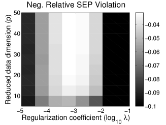
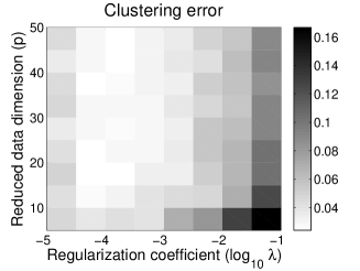
Figure 1: Relative SEP violation (left) and clustering error for Lasso SSC on the Hopkins-155 dataset. The rightmost two columns in the left figure indicate trivial solutions. White indicates good similarity graph or clustering and black indicates poor similarity graph or clustering.

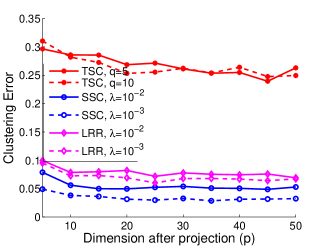
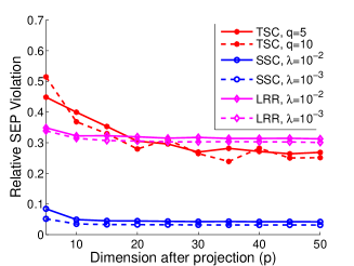
Figure 2: Comparison of clustering error (left) and relative SEP violation (right) for Lasso SSC, TSC and LRR on the Hopkins-155 dataset.

To gain some intuition into the performance of the SSC algorithm on dimensionality-reduced data, we report empirical results on Hopkins-155, a motion segmentation data set that is specifically designed to serve as a benchmark for subspace clustering algorithms (Tron & Vidal, 2007). The ambient dimension $d$ in the data set ranges from 112 to 240, and we compress the data points into $p$ dimension using random Gaussian projection, with $p$ taking the values from 5 to 50. We compare Lasso SSC with TSC (Heckel & Bolcskei, 2013) and LRR (Liu et al., 2013). The Lasso SSC algorithm is implemented using augmented Lagrangian method (ALM, Bertsekas (2014)). The LRR implementation is obtained from Liu (2013). All algorithms are implemented in Matlab.

For evaluation, we report both clustering error and the relative violation of the Self-Expressiveness Property (SEP). Clustering error is defined as the percentage of mis-clustered data points up to permutation. The relative violation of SEP characterizes how much the obtained similarity matrix $\mathbf{C}$ violates the self-expressiveness property. It was introduced in Wang & Xu (2013) and defined as

$$\text{RelViolation}(\mathbf{C},\mathcal{M})=\frac{\sum_{(i,j)\notin\mathcal{M}}{|\mathbf{C}|_{ij}}}{\sum_{(i,j)\in\mathcal{M}}{|\mathbf{C}|_{ij}}},$$ (2.8)

where $(i,j)\in\mathcal{M}$ means $\boldsymbol{x}_{i}$ and $\boldsymbol{x}_{j}$ belong to the same cluster and vice versa.

Figure 1 shows that the relative SEP violation of Lasso SSC goes up when the projection dimension $p$ decreases, or the regularization parameter $\lambda$ is too large or too small. The clustering accuracy acts accordingly. In addition, in Figure 2 we report the clustering error and relative SEP violation for Lasso SSC, TSC and LRR on Hopkins-155. Both clustering error and relative SEP violation are averaged across all 155 sequences. Figure 2 also indicates that Lasso SSC outperforms TSC and LRR under various regularization and projection dimension settings, which is consistent with previous experimental results (Elhamifar & Vidal, 2013).

3 Main results

We present general geometric success conditions for Lasso SSC on dimensionality-reduced data, under the fully deterministic setting where both the underlying low-dimensional subspaces and the data points on each subspace are placed deterministically. We first describe the result for the noiseless case and then the results are extended to handle a small amount of adversarial perturbation or a much larger amount of stochastic noise. In addition, implications of our success conditions under the much stronger semi-random and fully random models are discussed. The basic idea common in all of the upcoming results is to show that the subspace incoherence and inradius (therefore the geometric gap) are approximately preserved under dimension reduction.

3.1 Deterministic model: the noiseless case

We consider first the noiseless case where $\mathbf{Z}=\mathbf{0}$. We begin our analysis with two key concepts introduced in the seminal work of Soltanolkotabi et al. (2012): subspace incoherence and inradius. Subspace incoherence characterizes how well the subspaces associated with different clusters are separated. It is based on the dual direction of the optimization problem in Eq. (1.1) and (1.2), which is defined as follows:

Definition 3.1 (Dual direction, Soltanolkotabi et al., 2012; Wang & Xu, 2013).

Fix a column $\boldsymbol{x}$ of $\mathbf{X}$ belonging to subspace $\mathcal{U}^{(\ell)}$. Its dual direction $\boldsymbol{\nu}(\boldsymbol{x})$ is defined as the solution to the following dual optimization problem:

$$\max_{\boldsymbol{\nu}\in\mathbb{R}^{d}}{\langle\boldsymbol{x},\boldsymbol{\nu}\rangle-\frac{\lambda}{2}\boldsymbol{\nu}^{\top}\boldsymbol{\nu}},\quad\text{s.t. }\|\mathbf{X}^{\top}\boldsymbol{\nu}\|_{\infty}\leq 1.$$ (3.1)

Note that Eq. (3.1) has a unique solution when $\lambda>0$.

The subspace incoherence for $\mathcal{U}^{(\ell)}$, $\mu_{\ell}$, is defined in Eq. (3.2). Note that it is not related to the column subspace incoherence defined in Eq. (2.5). The smaller $\mu_{\ell}$ is the further $\mathcal{U}^{(\ell)}$ is separated from the other subspaces.

Definition 3.2 (Subspace incoherence, Soltanolkotabi et al. (2012); Wang & Xu (2013)).

Subspace incoherence $\mu_{\ell}$ for subspace $\mathcal{U}^{(\ell)}$ is defined as

$$\mu_{\ell}:=\max_{\boldsymbol{x}\in\mathbf{X}\backslash\mathbf{X}^{(\ell)}}{\|\mathbf{V}^{(\ell)\top}\boldsymbol{x}\|_{\infty}},$$ (3.2)

where $\mathbf{V}^{(\ell)}=(\boldsymbol{v}(\boldsymbol{x}_{1}^{(\ell)}),\cdots,\boldsymbol{v}(\boldsymbol{x}_{N_{\ell}}^{(\ell)}))$ and $\boldsymbol{v}(\boldsymbol{x})=\mathcal{P}_{\mathcal{U}^{(\ell)}}\boldsymbol{\nu}(\boldsymbol{x})/{\|\mathcal{P}_{\mathcal{U}^{(\ell)}}\boldsymbol{\nu}(\boldsymbol{x})\|_{2}}$. $\boldsymbol{\nu}(\boldsymbol{x})$ is the dual direction of $\boldsymbol{x}$ defined in Eq. (3.1) and $\mathcal{U}^{(\ell)}$ is the low-dimensional subspace on which $\boldsymbol{x}$ lies.

The concept of inradius characterizes how well data points are distributed within a single subspace. More specifically, we have the following definition:

Definition 3.3 (Inradius, Soltanolkotabi et al., 2012).

For subspace $\mathcal{U}^{(\ell)}$, its inradius $\rho_{\ell}$ is defined as

$$\rho_{\ell}:=\min_{i=1,\cdots,N_{\ell}}{r(\mathcal{Q}(\mathbf{X}_{-i}^{(\ell)}))},$$ (3.3)

where $r(\cdot)$ denotes the radius of the largest ball inscribed in a convex body.

The larger $\rho_{\ell}$ is, the more uniformly data points are distributed in the $\ell$th subspace. We also remark that both $\mu_{\ell}$ and $\rho_{\ell}$ are between 0 and 1 because of normalization.

With the characterization of subspace incoherence and inradius, we are now ready to present our main result, which states sufficient success condition for Lasso SSC on dimensionality-reduced noiseless data under the fully deterministic setting.

Theorem 3.1 (Compressed SSC on noiseless data).

Suppose $\mathbf{X}\in\mathbb{R}^{d\times N}$ is a noiseless input matrix with subspace incoherence $\{\mu_{\ell}\}_{\ell=1}^{k}$ and inradii $\{\rho_{\ell}\}_{\ell=1}^{k}$. Assume $\mu_{\ell}<\rho_{\ell}$ for all $\ell\in\{1,\cdots,k\}$. Let $\widetilde{\mathbf{X}}^{\prime}$ be the normalized data matrix after compression. Assume $0<\lambda<\rho/2$, where $\rho=\min_{\ell}\rho_{\ell}$. If $\mathbf{\Psi}$ satisfies Eq. (2.2,2.3) with parameter $\epsilon$ then Lasso SSC satisfies subspace detection property if $\epsilon$ is upper bounded by

$$\epsilon=O\left(\Delta^{2}\lambda^{3/2}\right),$$ (3.4)

where $\Delta=\min_{\ell}{(\rho_{\ell}-\mu_{\ell})}$ is the minimum gap between subspace incoherence and inradius for each subspace.

We make several remarks on Theorem 3.1. First, an upper bound on $\epsilon$ implies a lower bound about projection dimension $p$, and exact $p$ values vary for different data compression schemes. For example, if Gaussian random projection is used then $\epsilon=O(\Delta^{2}\lambda^{3/2})$ is satisfied with $p=\Omega(\Delta^{-2}\lambda^{3}r\log N)$. In addition, even for noiseless data the regularization coefficient $\lambda$ cannot be too small if projection error $\epsilon$ is present (recall that $\lambda\to 0$ corresponds to the exact SSC formulation). This is because when $\lambda$ goes to zero the strong convexity of the dual optimization problem decreases. As a result, small perturbation on $\mathbf{X}$ could result in drastic changes of the dual direction and Lemma 5.5 fails subsequently. On the other hand, as $\lambda$ increases the similarity graph connectivity decreases because the optimal solution to Eq. (1.2) becomes sparser. To guarantee the obtained solution is nontrivial (i.e., at least one nonzero entry in $\boldsymbol{c}_{i}$), $\lambda$ must not exceed $\rho/2$.

3.2 Deterministic model: the noisy case

When data are corrupted by either adversarial or stochastic noise, we can still hope to get success conditions for Lasso SSC provided that the magnitude of noise is upper bounded. The success conditions can again be stated using the concepts of subspace incoherence and inradius. Although the definition of subspace incoherence in Eq. (3.2) remains unchanged (i.e., defined in terms of the noisy data $\mathbf{X}$), the definition of inradius needs to be slightly adjusted under the noisy setting as follows:

Definition 3.4 (Inradius for noisy SSC, Wang & Xu (2013)).

Let $\mathbf{X}=\mathbf{Y}+\mathbf{Z}$ where $\mathbf{Y}$ is the uncorrupted data, $\mathbf{Z}$ is the noise matrix and $\mathbf{X}$ is the observation matrix. For subspace $\mathcal{U}^{(\ell)}$, its inradius $\rho_{\ell}$ is defined as

$$\rho_{\ell}:=\min_{i=1,\cdots,N_{\ell}}{r(\mathcal{Q}(\mathbf{Y}_{-i}^{(\ell)}))},$$ (3.5)

where $r(\cdot)$ denotes the radius of the largest ball inscribed in a convex body.

As a remark, under the noiseless setting we have $\mathbf{X}=\mathbf{Y}$ and Definition 3.4 reduces to the definition of inradius for noiseless data.

Finally, we have Theorem 3.2 and Theorem 3.3.

Theorem 3.2 (Compressed-SSC under deterministic noise).

Suppose $\mathbf{X}=\mathbf{Y}+\mathbf{Z}$ is a noisy input matrix with subspace incoherence $\{\mu_{\ell}\}_{\ell=1}^{k}$ and inradii $\{\rho_{\ell}\}_{\ell=1}^{k}$. Assume $\max_{i}{\|\boldsymbol{z}_{i}\|_{2}}\leq\eta$ and $\mu_{\ell}<\rho_{\ell}$ for all $\ell\in\{1,\cdots,k\}$. Suppose $\widetilde{\mathbf{X}}^{\prime}=\widetilde{\mathbf{Y}}^{\prime}+\widetilde{\mathbf{Z}}$ where $\widetilde{\mathbf{Y}}^{\prime}$ is the normalized uncorrupted data matrix after compression and $\widetilde{\mathbf{Z}}=\mathbf{\Psi}\mathbf{Z}$ is the projected noise matrix. If $\mathbf{\Psi}$ satisfies Eq. (2.2,2.3) with parameter $\epsilon$ and $\lambda$ satisfies

$$\frac{24\eta}{\Delta}<\lambda<\rho(1-\epsilon)-6\eta,$$ (3.6)

then Lasso SSC satisfies the subspace detection property if the approximation error $\epsilon$ and noise magnitude $\eta$ satisfy

$$\max(\epsilon,\eta)=O\left(\Delta^{2}\lambda^{3/2}\right).$$ (3.7)

Here $\Delta=\min_{\ell}{(\rho_{\ell}-\mu_{\ell})}$ is the minimum gap between subspace incoherence and inradius.

Theorem 3.3 (Compressed-SSC under stochastic noise).

Suppose $\mathbf{X}=\mathbf{Y}+\mathbf{Z}$ is a noisy input matrix with subspace incoherence $\{\mu_{\ell}\}_{\ell=1}^{k}$ and inradii $\{\rho_{\ell}\}_{\ell=1}^{k}$. Assume $\mathbf{Z}_{ij}\sim\mathcal{N}(0,\frac{\sigma^{2}}{d})$ for some noise magnitude parameter $\sigma$. Suppose $\widetilde{\mathbf{X}}^{\prime}=\widetilde{\mathbf{Y}}^{\prime}+\widetilde{\mathbf{Z}}$ where $\widetilde{\mathbf{Y}}^{\prime}$ is the normalized uncorrupted data matrix after compression and $\widetilde{\mathbf{Z}}=\mathbf{\Psi}\mathbf{Z}$ is the projected noise matrix. If the spectral norm of $\mathbf{\Psi}\in\mathbb{R}^{p\times d}$ is upper bounded by $\|\mathbf{\Psi}\|_{2}\leq\psi\sqrt{\frac{d}{p}}$ for some constant $\psi$ (i.e., $\psi=O(1)$) and in addition $\mathbf{\Psi}$ satisfies Eq. (2.2,2.3) with parameter $\epsilon$ and $\lambda$ satisfies

$$C_{1}\cdot\frac{\sigma(1+\sigma)}{\Delta}\sqrt{\frac{\log N}{d}}<\lambda<\frac{\rho}{2}-C_{2}\cdot\sigma(1+\sigma)\sqrt{\frac{\log N}{d}}$$ (3.8)

for some universal constants $C_{1},C_{2}>0$, then Lasso SSC satisfies the subspace detection property if the approximation error $\epsilon$ and noise magnitude $\sigma$ satisfy

$$\epsilon=O\left(\Delta^{2}\lambda^{3/2}\right),\quad\sigma=O\left(\min\left\{\frac{\Delta^{1/2}\lambda^{1/2}d^{1/4}}{\log^{1/4}N},\frac{\Delta\rho^{1/2}d^{1/4}}{r^{1/4}\log^{5/4}N},\frac{\Delta^{2}\lambda^{3/2}d^{1/2}}{r^{1/2}\log^{3/2}N}\right\}\right),$$ (3.9)

where $\Delta=\min_{\ell}{(\rho_{\ell}-\mu_{\ell})}$ is the minimum gap between subspace incoherence and inradius.

Before we proceed some clarification on the ambient data dimension $d$ is needed. Eq. (3.9) seems to suggest that the noise variance $\sigma$ increases with $d$. While this is true if noise magnitude is measured in terms of the $\ell_{2}$ norm $\|\boldsymbol{z}\|_{2}$, we remark that coordinate-wise noise variance does not increase with $d$, because each one of the $d$ coordinates of $z$ is a Gaussian random variable with variance $\sigma^{2}/d$.

These results put forward an interesting view of the subspace clustering problem in terms of resource allocation. The critical geometric gap $\Delta$ (called “Margin of Error” in Wang & Xu (2013)) can be viewed as the amount of resource that we have for a problem while preserving the subspace detection property. It can be used to tolerate noise, compress the data matrix, or alleviate the graph connectivity problem of SSC Wang et al. (2013). With larger geometric gap $\Delta$, the approximation error $\epsilon$ from dimensionality reduction can be tolerated at a larger level, which implies that the original data $\mathbf{X}$ can be compressed more aggressively, at a smaller dimension $p$ after compression, without losing the SDP property of sparse subspace clustering. The results also demonstrate trade-offs between noise tolerance and dimensionality reduction. For example, at a higher level of noise variance $\sigma$ or $\eta$ the regularization parameter $\lambda$ must be set at a lower level, according to conditions in Eqs. (3.6,3.8); subsequently, the approximation error $\epsilon$ in dimensionality reduction needs to be smaller to ensure success of SSC on the projected data, which places a higher lower bound on the dimension $p$ one can compress the original data into.

3.3 Semi-random and Fully-random models

In this section we consider random data models, where either the data points or the underlying low-dimensional subspaces are assumed to be drawn i.i.d. from a uniform distribution. Under the semi-random model the underlying subspaces $\mathcal{U}^{(\ell)}$, $\ell=1,\cdots,k$ are still assumed to be fixed but unknown. However, we place stochastic conditions on the data points by assuming that each data point is drawn uniformly at random from the unit sphere of the corresponding low-dimensional subspace. This assumption makes the success conditions of Lasso SSC more transparent, as the success conditions now only depend on the number of data points per subspace and the affinity between different subspaces, which is formally defined as follows:

Definition 3.5 (Subspace affinity (normalized), (Soltanolkotabi et al., 2012; Wang & Xu, 2013)).

For two subspaces $\mathcal{U}^{(\ell)},\mathcal{U}^{(\ell^{\prime})}$ of intrinsic dimension $r_{\ell}$ and $r_{\ell^{\prime}}$, the affinity between $\mathcal{U}^{(\ell)}$ and $\mathcal{U}^{(\ell^{\prime})}$ is defined as

$$\mathrm{aff}_{\mathrm{N}}(\mathcal{U}^{(\ell)},\mathcal{U}^{(\ell^{\prime})})=\sqrt{\frac{\cos^{2}(\theta_{1})+\cdots+\cos^{2}(\theta_{r_{\ell}\wedge r_{\ell^{\prime}}})}{r_{\ell}r_{\ell^{\prime}}}},$$ (3.10)

where $\theta_{1},\cdots,\theta_{r_{\ell}\wedge r_{\ell^{\prime}}}$ are canonical angles between $\mathcal{U}^{(\ell)}$ and $\mathcal{U}^{(\ell^{\prime})}$. Note that $\mathrm{aff}_{\mathrm{N}}(\mathcal{U}^{(\ell)},\mathcal{U}^{(\ell^{\prime})})$ is always between 0 and 1, with smaller value indicating one subspace being further apart from the other.

We are now able to state our main theorem on success conditions of dimensionality-reduced noisy SSC under the semi-random model.

Theorem 3.4 (Compressed SSC under Semi-random Model).

Suppose $\mathbf{X}=\mathbf{Y}+\mathbf{Z}$ is a noisy input matrix with $\mathbf{Y}^{(\ell)}$ sampled uniformly at random from the unit sphere in $\mathcal{U}^{(\ell)}$ and $\mathbf{Z}_{ij}\sim\mathcal{N}(0,\frac{\sigma^{2}}{d})$ for some noise magnitude parameter $\sigma$. Assume in addition that $N_{\ell}\geq\kappa r_{\ell}$ for some $\kappa>1$ and the subspace affinity $\{\mathrm{aff}_{\mathrm{N}}(\mathcal{U}^{(\ell)},\mathcal{U}^{(\ell^{\prime})})\}_{\ell,\ell^{\prime}=1}^{k}$ satisfies

$$\min_{\ell^{\prime}\neq\ell}\mathrm{aff}_{\mathrm{N}}(\mathcal{U}^{(\ell)},\mathcal{U}^{(\ell^{\prime})})=O\left(\frac{1}{\log^{2}(kN)}\sqrt{\frac{\log\kappa}{r}}\right),\;\;\;\;\forall\ell=1,\cdots,k.$$ (3.11)

Suppose $\widetilde{\mathbf{X}}^{\prime}=\widetilde{\mathbf{Y}}^{\prime}+\widetilde{\mathbf{Z}}$ where $\widetilde{\mathbf{Y}}^{\prime}$ is the normalized uncorrupted data matrix after compression and $\widetilde{\mathbf{Z}}=\mathbf{\Psi}\mathbf{Z}$ is the projected noise matrix. If the spectral norm of $\mathbf{\Psi}\in\mathbb{R}^{p\times d}$ is upper bounded by $\|\mathbf{\Psi}\|_{2}\leq\psi\sqrt{\frac{d}{p}}$ for some constant $\psi$ (i.e., $\psi=O(1)$) and in addition $\mathbf{\Psi}$ satisfies Eq. (2.2,2.3) with parameter $\epsilon$ and $\lambda\asymp\sqrt{\log\kappa/r}$, then Lasso SSC satisfies the subspace detection property with probability $\geq 1-O(1/N)$ if the approximation error $\epsilon$ and noise magnitude $\sigma$ satisfy

$$\epsilon=O\left(\frac{\log^{7/4}\kappa}{r^{7/4}}\right),\;\;\;\;\sigma=O\left(\min\left\{\frac{d^{1/4}\log^{3/4}\kappa}{r\log^{5/4}N},\frac{d^{1/2}\log^{7/4}\kappa}{r^{9/4}\log^{3/2}N}\right\}\right).$$ (3.12)

Furthermore, as a corollary, if $\mathbf{\Psi}\in\mathbb{R}^{p\times d}$ is the random Gaussian projection matrix (i.e., $\mathbf{\Psi}_{ij}\sim\mathcal{N}(0,1/p)$) with $p$ the dimension after projection, then Lasso SSC satisfies the subspace detection property with probability $\geq 1-O(1/N)$ if the noise magnitude $\sigma$ satisfies the constraint as in Eq. (3.12) and the projected dimension $p$ is at least

$$p=\Omega\left(r^{9/2}\cdot\frac{\log(kN)}{\log^{7/2}\kappa}\right).$$ (3.13)

As a remark, Theorem 3.13 shows that using the Gaussian random projection operator, the dimension after projection $p$ depends polynomially on the intrinsic dimension $r$. Such dependency is unavoidable, as one cannot hope to compress the data to the point that data dimension after compression is smaller than the intrinsic dimension. On the other hand, our analysis shows that $p$ depends only poly-logarithmically on both the number of subspaces $k$ and the number of data points $N$. Such dependency is significantly better than treating the entire union-of-subspace model as an agglomerate low-rank model, which would then require $\Omega(kr\log N)$ dimension after compression. However, we conjecture the $r^{9/2}$ term in Eq. (3.13) is loose (which comes up in our argument of strong convexity of the dual problem of SSC) and could be improved to an even lower order of polynomial function. Finally, we note that $p$ needs to increase with $N$, the total number of data points, which might seem counter-intuitive. This is because success of the SSC algorithm is defined in terms of self-expressiveness property over all data points, which becomes more difficult to satisfy with more data points.

We next turn to the fully-random model, where not only the data points but also the underlying subspaces $\mathcal{U}^{(1)},\cdots,\mathcal{U}^{(k)}$ are assumed to be drawn i.i.d. uniformly at random. In this even simpler model, we have the following theorem that directly follows from Theorem 3.13:

Theorem 3.5 (Compressed SSC under fully random model).

With the same notation and conditions in Theorem 3.13, except that the condition on subspace affinity, Eq. (3.11), is replaced by the following condition that involves only the number of data points $N$, the ambient dimension $d$ and the data ratio $\kappa$:

$$r=O\left(\frac{d\log\kappa}{\log N}\right).$$ (3.14)

Then under the random Gaussian projection operator, Lasso SSC succeeds with probability $\geq 1-O(1/N)$ if $\lambda\asymp\sqrt{\log(\kappa)/r}$ and the number of dimension after compression $p$ satisfies

$$p=\Omega\left(r^{9/2}\cdot\frac{\log(kN)}{\log^{7/2}\kappa}\right).$$ (3.15)

4 Application to privacy preserving subspace clustering

Dimensionality reduction is useful in many practical applications involving subspace clustering, as explained in the introduction. In this section, we discuss one particular motivation of compressing data before data analysis in order to protect data privacy. The privacy issue of subspace clustering has received research attention recently (Wang et al., 2015b), as it is applied to sensitive data sets such as medical/genetic or movie recommendation data (Zhang et al., 2012; McWilliams & Montana, 2014). Nevertheless, there has been no prior work on formally establishing privacy claims for sparse subspace clustering algorithms.

In this section we investigate differentially private sparse subspace clustering under a random projection dimension reduction model. This form of privacy protection is called “matrix masking” and has a long history in statistical privacy and disclosure control (see, e.g., Duncan et al., 1991; Willenborg & De Waal, 1996; Hundepool et al., 2012). It has been formally shown more recently that random projections (at least with Gaussian random matrices) protect information privacy (Zhou et al., 2009). Stronger privacy protection can be enforced by injecting additional noise to the dimension reduced data (Kenthapadi et al., 2013). Algorithmically, this basically involves adding iid Gaussian noise to the data after we apply a Johnson-Lindenstrauss transform $\mathbf{\Psi}$ of choice to $\mathbf{X}$ and normalize every column. This procedure guarantees differential privacy (Dwork et al., 2006; Dwork, 2006) at the attribute level, which prevents any single entry of the data matrix from being identified “for sure” given the privatized data and arbitrary side information. The amount of noise to add is calibrated according to how “unsure” we need to be and how “spiky” (Definition 2.2) each data point can be. We show in Sec. 4.1 and 4.2 that the proposed variant of SSC algorithm achieves perfect clustering with high probability while subject to formal privacy constraints. We also prove in Sec. 4.3 that a stronger user-level privacy constraint cannot be attained when perfect clustering of each data point is required. Wang et al. (2015b) discussed alternative solutions to this dilemma by weakening the utility claims.

4.1 Privacy claims

In classic statistical privacy literature, transforming data set $\mathbf{X}$ by taking $\tilde{\mathbf{X}}=\mathbf{A}\mathbf{X}+\mathbf{E}$ for some random matrix $\mathbf{A}$ and $\mathbf{E}$ is called matrix masking. Zhou et al. (2009) show that random compression allows the mutual information of the output $\tilde{\mathbf{X}}$ and raw data $\mathbf{X}$ to converge to $0$ with rate $O(p/d)$ even when $\mathbf{M}=0$, and their result directly applies to our problem. The guarantee suggests that the amount of information in the compressed output $\tilde{\mathbf{X}}$ about the raw data $\mathbf{X}$ goes to 0 as the ambient dimension $d$ gets large.

On the other hand, if $\mathbf{E}\neq\mathbf{0}$ is an iid Gaussian noise matrix, we can protect the $(\varepsilon,\delta)$-differential privacy of every data entry. More specifically, we view the matrix $\mathbf{X}$ as a data collection of $N$ users, each corresponding to a column in $\mathbf{X}$ associated with a $d$-dimensional attribute vector. Each entry in $\mathbf{X}$ then corresponds to a particular attribute of a specific user. The formal definition of attribute differential privacy notion is given below:

Definition 4.1 (Attribute Differential Privacy).

Suppose $\mathcal{O}$ is the set for all possible outcomes. We say a randomized algorithm $\mathcal{A}:\mathbb{R}^{d\times N}\rightarrow\mathcal{O}$ is $(\varepsilon,\delta)$-differentially private at attribute level if

$$\Pr(\mathcal{A}(\mathbf{X})\in\mathcal{S})\leq e^{\varepsilon}\Pr(\mathcal{A}(\mathbf{X}^{\prime})\in\mathcal{S})+\delta$$

for any measurable outcome $\mathcal{S}\subset\mathcal{O}$, any $\mathbf{X}$ and $\mathbf{X}^{\prime}$ that differs in only one entry.

This is a well-studied setting in (Kenthapadi et al., 2013). It is weaker than protecting the privacy of individual users (i.e., entire columns in $\mathbf{X}$), but much stronger than the average protection via mutual information. In fact, it forbids any feature of an individual user from being identified “for sure” by an adversary with arbitrary side information.

Theorem 4.1.

Assume the data (and all other users that we need to protect) satisfy column spikiness conditions with parameter $\mu_{0}$ as in Definition 2.2. Let $\mathbf{\Psi}$ be a Johnson-Lindenstrauss transform with parameter $\epsilon$. Releasing compressed data $\widetilde{\mathbf{X}}^{\prime}=\mathrm{Normalize}(\mathbf{\Psi}\mathbf{X})+\mathcal{N}(0,\sigma^{2}/d\cdot\mathbf{I}_{p\times d})$ with $\sigma=\frac{1+\epsilon}{1-\epsilon}\sqrt{\frac{32\mu_{0}\log(1.25/\delta)}{\varepsilon^{2}}}$ preserves attribute-level $(\varepsilon,\delta)$-differential privacy.

Note that in Theorem 4.1 the exact value of $\mu_{0}$ is not necessary: an upper bound of $\mu_{0}$ would be sufficient, which results in more conservative differentially private procedures.

The proof involves working out the $\ell_{2}$-sensitivity of the operator $\text{Normalize}(\mathbf{\Psi}(\cdot))$ in terms of column incoherence $\mu_{0}$ and apply “Gaussian Mechanism” (Dwork, 2006; Dwork & Roth, 2013). We defer the proof to Sec. 5.6. Note that differential privacy is close to “post-processing”, meaning that any procedure on the released data does not change the privacy level. Therefore, applying SSC on the released data $\widetilde{\mathbf{X}}^{\prime}$ injected with noise remains a $(\epsilon,\delta)$-differentially private procedure.

4.2 Utility claims

We show that if column spikiness $\mu_{0}$ is a constant, Lasso-SSC is able to provably detect the correct subspace structures, despite privacy constraints.

Corollary 4.1.

Let the raw data $\mathbf{X}$ be compressed and privatized using the above described mechanism to get $\widetilde{\mathbf{X}}$. Assume the same set of notations and assumptions in Theorem 3.1. Suppose $\mathbf{\Psi}$ is a JL transform with parameter $\epsilon$. Let $B:=\min_{\ell=1,...,k}\{\rho,r^{-1/2},\rho_{\ell}-\mu_{\ell}\}$. If the privacy parameter $\varepsilon$ satisfies

$$\varepsilon=\Omega\left(\sqrt{\frac{\mu_{0}\log(1/\delta)}{d}}\cdot\max\left\{\frac{\log^{5/4}{N}}{B^{2}},\frac{\log^{3/2}{N}}{B^{11/2}p^{1/4}}\right\}\right),$$ (4.1)

then the solution to Lasso-SSC using obeys the subspace detection property with probability $1-8/N-\delta$.

Corollary 4.1 should be interpreted with care: though we place a lower bound condition on the privacy parameter $\varepsilon$, which might sound strange because $\varepsilon$ is usually specified by users, such lower bound condition is only required to establish utility guarantees. The algorithm itself is always ($\varepsilon,\delta)$-differential private regardless of $\varepsilon$ values, as stated in Theorem 4.1. On the other hand, if the original data $\mathbf{X}$ is sufficiently incoherent (i.e., $\mu_{0}=O(1)$), the right-hand side of Eq. (4.1) scales as $O(\mathrm{poly}(r)/\sqrt{d})$, which quickly approaches zero as the ambient dimension $d$ increases. As a result, the lower bound in Eq. (4.1) is a very mild condition on incoherent data matrix $\mathbf{X}$.

The proof idea of Corollary 4.1 is simple. We are now injecting artificial Gaussian noise to a compressed subspace clustering problem with fixed input, and Theorem 3.3 directly addresses that. All we have to do is to replace the geometric quantities in $\mu_{\ell}$ and $\rho_{\ell}$ by their respective bound after compression in Corollary 5.1 and Lemma 5.2. The complete proof is deferred to Sec. 5.7.

Before proceeding to the impossibility results we make some remarks on the condition of the privacy parameter $\varepsilon$. It can be seen that, smaller privacy parameter (i.e., higher degree of privacy protection) is possible on data sets with larger “geometric gap” that makes subspace clustering relatively easy to succeed on such data sets. In addition, incoherence helps with privacy preservation, as $\varepsilon$ can be set at a smaller level on more incoherent data.

4.3 Impossibility results

As we described in the main results, attribute-level differential privacy is a much weaker notion of privacy. A stronger privacy notion is user-level differential privacy, where two neighboring databases $\mathbf{X}$ and $\mathbf{X}^{\prime}$ differ by a column rather than an entry, and hence the privacy of the entire attribute vector of each user in $\mathbf{X}$ is protected. However, we show in this section that user-level differential privacy cannot be achieved if utility is measured in terms of (perfect) subspace detection property.

We first give a formal definition of user-level differential privacy:

Definition 4.2 (User-Level Differential Privacy).

We say a randomized algorithm $\mathcal{A}:\mathbb{R}^{d\times N}\rightarrow\mathcal{O}$ is $(\varepsilon,\delta)$-differential private at user level if

$$\Pr(\mathcal{A}(\mathbf{X})\in\mathcal{S})\leq e^{\varepsilon}\Pr(\mathcal{A}(\mathbf{X}^{\prime})\in\mathcal{S})+\delta$$

for any measurable outcome $\mathcal{S}\subset\mathcal{O}$, any $\mathbf{X},\mathbf{X}^{\prime}\in\mathcal{X}^{n}$ that differs in only one column.

Compared with the attribute differential privacy defined in 4.1, the only difference is how $\mathbf{X}$ and $\mathbf{X}^{\prime}$ may differ. Note that we can arbitrarily replace any single point in $\mathbf{X}$ with any $x\in\mathcal{X}$, to form $\mathbf{X}^{\prime}$.

The following proposition shows that user-level differential privacy cannot be preserved if perfect subspace detection or clustering is desired. Its proof is placed in Sec. 5.8.

Proposition 4.1.

User-level differential privacy is NOT possible for any $0\leq\varepsilon<\infty$ using any privacy mechanism if perfect subspace detection property or perfect clustering results are desired. In addition, If an algorithm achieves perfect clustering or subspace detection with probability $1-\delta$ for some $\delta\in(0,1)$, user-level differential privacy is NOT possible for any $\varepsilon<\log\left(\frac{1-\delta}{\delta}\right)$.

Intuitively, the reason why attribute-level privacy is not subject to the impossibility result in Proposition 4.1 is because the privacy promise is much weaker: even if perfect subspace detection or clustering results are presented, it is still possible to hide the information of a specific attribute of a user provided that the attribute values are distributed in a incoherent and near-uniform way. On the other hand, change in a user’s complete attribute file may often alter the cluster that user belongs to and eventually break perfect subspace clustering.

User-level privacy for sparse subspace clustering and for privacy in general remains an important open problem. Some progress has been made in Wang et al. (2015b) to address user-level private subspace clustering by weakening the utility guarantee from correct clustering to approximately identifying underlying subspaces. Nevertheless, the analysis in Wang et al. (2015b) mostly focus on simpler algorithms like thresholding-based subspace clustering (Heckel & Bolcskei, 2013) and cannot be easily generalized to state-of-the-art subspace clustering methods such as SSC (Elhamifar & Vidal, 2013) or LRR (Liu et al., 2013).

5 Proofs

Success condition for exact SSC was proved in Soltanolkotabi et al. (2012) and was generalized to the noisy case in Wang & Xu (2013). Below we cite Theorem 6 and Theorem 8 in Wang & Xu (2013) for a success condition of Lasso SSC. In general, Lasso SSC succeeds when there is a sufficiently large gap between subspace incoherence and inradius. Results are restated below, with minor simplification in our notation.

Theorem 5.1 (Wang & Xu, 2013, Theorem 6 and 8).

Suppose $\mathbf{X}=\mathbf{Y}+\mathbf{Z}$ where $\mathbf{Y}$ is the uncorrupted data matrix and $\mathbf{Z}=(\boldsymbol{z}_{1},\cdots,\boldsymbol{z}_{N})$ is a deterministic noise matrix that satisfies $\max_{i=1}^{N}{\|\boldsymbol{z}_{i}\|_{2}}\leq\eta$. Define $\rho:=\min_{\ell}{\rho_{\ell}}$. If

$$\eta\leq\min_{\ell=1,\cdots,k}{\frac{\rho(\rho_{\ell}-\mu_{\ell})}{7\rho_{\ell}+2}},$$ (5.1)

then subspace detection property holds for the Lasso SSC algorithm in Eq. (1.2) if the regularization coefficient $\lambda$ is in the range

$$\max_{\ell=1,\cdots,k}{\frac{\eta(1+\eta)(2+\rho_{\ell})}{\rho_{\ell}-\mu_{\ell}-2\eta}}<\lambda<\rho-2\eta-\eta^{2}.$$ (5.2)

In addition, if $\mathbf{Z}_{ij}\sim\mathcal{N}(0,\sigma_{ij}^{2}/d)$ are independent Gaussian noise with variance $\sigma^{2}:=\max_{i,j}\sigma_{ij}^{2}$ satisfying

$$\sqrt{\frac{\log N}{d}}\sigma(1+\sigma)<C\min_{\ell=1,\cdots,k}\left\{\rho,r^{-1/2},\rho_{\ell}-\mu_{\ell}\right\}$$ (5.3)

for sufficiently small constant $C\geq 1/80$, then with probability at least $1-\frac{10}{N}$ the subspace detection property holds if $\lambda$ is in the range

$$\frac{C_{1}\sigma(1+\sigma)}{\rho_{\ell}-\mu_{\ell}}\sqrt{\frac{\log N}{d}}<\lambda<\rho-C_{2}\sigma(1+\sigma)\sqrt{\frac{\log N}{d}}.$$ (5.4)

Here $C_{1}\leq 80$ and $C_{2}\leq 20$ are absolute constants.

5.1 Proof of Theorem 3.1

We first bound the perturbation of dual directions when the data are noiseless.

Lemma 5.1 (Perturbation of dual directions, the noiseless case).

Assume $0<\lambda<1$. Fix a column $\boldsymbol{x}$ in $\mathbf{X}$ with dual direction $\boldsymbol{\nu}=\boldsymbol{\nu}(\boldsymbol{x})$ and $\boldsymbol{v}=\boldsymbol{v}(\boldsymbol{x})$ defined in Eq. (3.1) and (3.2). Let $\widetilde{\mathbf{X}}$ denote the projected data matrix $\mathbf{\Psi}\mathbf{X}$ and $\widetilde{\mathbf{X}}^{\prime}$ denote the normalized version of $\widetilde{\mathbf{X}}$. Suppose $\boldsymbol{\nu}^{*}$ and $\boldsymbol{v}^{*}$ are computed using the normalized projected data matrix $\widetilde{\mathbf{X}}^{\prime}$. If $\mathbf{\Psi}$ satisfies Eq. (2.2, 2.3) with parameter $\epsilon$ and $\epsilon<1/2\max(1,\|\boldsymbol{\nu}\|^{2})$ then the following holds for all $\boldsymbol{w}\in\mathbf{X}\backslash\mathbf{X}^{(\ell)}$:

$$\big{|}\langle\boldsymbol{v},\boldsymbol{w}\rangle-\langle\boldsymbol{v}^{*},\tilde{\boldsymbol{w}}^{\prime}\rangle\big{|}=O\left(\epsilon^{1/2}\lambda^{-3/4}\right).$$ (5.5)

Proof.

Fix $\ell\in[k]$ and one column $\boldsymbol{x}_{i}$ in $\mathbf{X}$. Let $\mathcal{U}^{(\ell)}$ and $\widetilde{\mathcal{U}}^{(\ell)}$ denote the low-rank subspaces to which $\boldsymbol{x}_{i}$ belongs before and after compression. That is, $\widetilde{\mathcal{U}}^{(\ell)}=\{\mathbf{\Psi}\boldsymbol{x}:\boldsymbol{x}\in\mathcal{U}^{(\ell)}\}$.

First note that $(1-\lambda/2)^{2}\leq\|\boldsymbol{\nu}\|^{2}\leq 2/\lambda$. $\|\boldsymbol{\nu}\|\geq 1-\lambda/2$ because $\langle\boldsymbol{x},\boldsymbol{\nu}\rangle-\lambda/2\cdot\|\boldsymbol{\nu}\|^{2}\leq\langle\boldsymbol{x},\boldsymbol{\nu}\rangle\leq\|\boldsymbol{\nu}\|$ and putting $\boldsymbol{\nu}=\boldsymbol{x}$ we obtain a solution with value $1-\lambda/2$. On the other hand, $\langle\boldsymbol{x},\boldsymbol{\nu}\rangle-\lambda/2\cdot\|\boldsymbol{\nu}\|^{2}\leq\|\boldsymbol{\nu}\|-\lambda/2\cdot\|\boldsymbol{\nu}\|^{2}$ and putting $\boldsymbol{\nu}=\boldsymbol{0}$ we obtain a solution with value 0. Also, under the noiseless setting $\boldsymbol{\nu}\in\mathcal{U}^{(\ell)}$, if $\boldsymbol{x}\in\mathcal{U}^{(\ell)}$.

Define

$$\tilde{\boldsymbol{\nu}}^{\prime}=\frac{\sqrt{1-\epsilon}}{1+\epsilon\max(1,\|\boldsymbol{\nu}\|^{2})}\cdot\tilde{\boldsymbol{\nu}},$$

where $\tilde{\boldsymbol{\nu}}=\mathbf{\Psi}\boldsymbol{\nu}$. Let $f(\boldsymbol{\nu})=\langle\boldsymbol{\nu},\boldsymbol{x}\rangle-\frac{\lambda}{2}\|\boldsymbol{\nu}\|_{2}^{2}$ and $\tilde{f}(\tilde{\boldsymbol{\nu}}^{\prime})=\langle\tilde{\boldsymbol{\nu}}^{\prime},\tilde{\boldsymbol{x}}^{\prime}\rangle-\frac{\lambda}{2}\|\tilde{\boldsymbol{\nu}}^{\prime}\|_{2}^{2}$ denote the values of the optimization problems. The first step is to prove that $\tilde{\boldsymbol{\nu}}$ is feasible and nearly optimal to the projected optimization problem; that is, $\tilde{f}(\tilde{\boldsymbol{\nu}}^{\prime})$ is close to $\tilde{f}(\boldsymbol{\nu}^{*})$.

We first show that $\tilde{\boldsymbol{\nu}}^{\prime}$ is a feasible solution with high probability. By Proposition 2.3, the following bound on $|\tilde{\boldsymbol{x}}_{i}^{\top}\tilde{\boldsymbol{\nu}}|$ holds:

$$|\tilde{\boldsymbol{x}}_{i}^{\top}\tilde{\boldsymbol{\nu}}|\leq|\boldsymbol{x}_{i}^{\top}\boldsymbol{\nu}|+\epsilon\cdot\frac{\|\boldsymbol{x}_{i}\|^{2}+\|\boldsymbol{\nu}\|^{2}}{2}\leq 1+\epsilon\max(1,\|\boldsymbol{\nu}\|^{2}).\quad\forall\boldsymbol{x}_{i}\in\mathbf{X}.$$ (5.6)

Furthermore, with probability $\geq 1-\delta$

$$\|\tilde{\boldsymbol{x}}_{i}\|_{2}^{2}\geq(1-\epsilon)\|\boldsymbol{x}_{i}\|_{2}^{2}=1-\epsilon.$$ (5.7)

Consequently, by the definition of $\tilde{\boldsymbol{\nu}}^{\prime}$ one has

$$\|\widetilde{\mathbf{X}}^{\prime\top}\tilde{\boldsymbol{\nu}}^{\prime}\|_{\infty}\leq\frac{1}{\sqrt{1-\epsilon}}\cdot\frac{\sqrt{1-\epsilon}}{1+\epsilon\max(1,\|\boldsymbol{\nu}\|^{2})}\|\widetilde{\mathbf{X}}^{\top}\tilde{\boldsymbol{\nu}}\|_{\infty}\leq 1.$$ (5.8)

Next, we compute a lower bound on $\tilde{f}(\tilde{\boldsymbol{\nu}}^{\prime})$, which should serve as a lower bound for $\tilde{f}(\boldsymbol{\nu}^{*})$ because $\boldsymbol{\nu}^{*}$ is the optimal solution to the dual optimization problem on the projected data. We first remark that $\langle\boldsymbol{x},\boldsymbol{\nu}\rangle\geq 1-\lambda/2$ due to the optimality condition of the dual problem at $\boldsymbol{\nu}=\boldsymbol{x}$ and hence

$$\langle\tilde{\boldsymbol{x}},\tilde{\boldsymbol{\nu}}\rangle\geq\langle\boldsymbol{x},\boldsymbol{\nu}\rangle-\epsilon\cdot\frac{\|\boldsymbol{x}\|^{2}+\|\boldsymbol{\nu}\|^{2}}{2}\geq 1-\frac{\lambda}{2}-\epsilon\max(1,\|\boldsymbol{\nu}\|^{2})\geq 0,$$

where the last inequality is due to the assumption that $\lambda\in(0,1)$ and $\epsilon<1/2\max(1,\|\boldsymbol{\nu}^{2}\|)$. Consequently, we have the following chain of inequalities:

$$\tilde{f}(\tilde{\boldsymbol{\nu}}^{\prime}) = \langle\tilde{\boldsymbol{x}}^{\prime},\tilde{\boldsymbol{\nu}}^{\prime}\rangle-\frac{\lambda}{2}\|\tilde{\boldsymbol{\nu}}^{\prime}\|_{2}^{2}$$ (5.9)

$$\geq \sqrt{\frac{1-\epsilon}{1+\epsilon}}\frac{\langle\tilde{\boldsymbol{x}},\tilde{\boldsymbol{\nu}}\rangle}{1+\epsilon\max(1,\|\boldsymbol{\nu}\|^{2})}-\frac{\lambda}{2}(1-\epsilon)\|\tilde{\boldsymbol{\nu}}\|_{2}^{2}$$

$$\geq (1-\epsilon)(1-\epsilon\max(1,\|\boldsymbol{\nu}\|^{2}))\left(\langle\boldsymbol{x},\boldsymbol{\nu}\rangle-\epsilon\max(1,\|\boldsymbol{\nu}\|^{2})\right)-\frac{\lambda}{2}(1-\epsilon)(1+\epsilon)\|\boldsymbol{\nu}\|^{2}$$

$$\geq (1-\epsilon)(\langle\boldsymbol{x},\boldsymbol{\nu}\rangle-\epsilon\max(1,\|\boldsymbol{\nu}\|^{2}))-\epsilon\max(1,\|\boldsymbol{\nu}\|^{2})\cdot\langle\boldsymbol{x},\boldsymbol{\nu}\rangle-\frac{\lambda}{2}\|\boldsymbol{\nu}\|^{2}$$

$$\geq \langle\boldsymbol{x},\boldsymbol{\nu}\rangle-\epsilon\max(1,\|\boldsymbol{\nu}\|^{2})-\epsilon\langle\boldsymbol{x},\boldsymbol{\nu}\rangle-\epsilon\max(1,\|\boldsymbol{\nu}\|^{2})\cdot\langle\boldsymbol{x},\boldsymbol{\nu}\rangle-\frac{\lambda}{2}\|\boldsymbol{\nu}\|^{2}$$

$$\geq \langle\boldsymbol{x},\boldsymbol{\nu}\rangle-\epsilon\max(1,\|\boldsymbol{\nu}\|^{2})-\epsilon\|\boldsymbol{\nu}\|-\epsilon\max(1,\|\boldsymbol{\nu}\|^{2})\cdot\|\boldsymbol{\nu}\|-\frac{\lambda}{2}\|\boldsymbol{\nu}\|^{2}$$

$$\geq f(\boldsymbol{\nu})-3\epsilon\max(1,\|\boldsymbol{\nu}\|,\|\boldsymbol{\nu}\|^{2},\|\boldsymbol{\nu}\|^{3})$$

$$\geq f(\boldsymbol{\nu})-3\epsilon\max(1,\|\boldsymbol{\nu}\|^{3}).$$ (5.10)

On the other hand, since $\boldsymbol{\nu}^{*}\in\widetilde{\mathcal{U}}^{(\ell)}$, there exists $\bar{\boldsymbol{\nu}}\in\mathcal{U}^{(\ell)}$ such that $\boldsymbol{\nu}^{*}=\mathbf{\Psi}\bar{\boldsymbol{\nu}}$. Let $\bar{\boldsymbol{\nu}}^{\prime}$ be a scaled version of $\bar{\boldsymbol{\nu}}$ so that it is a feasible solution to the optimization problem in Eq. (3.1) before projection. Using essentially similar analysis one can show that $f(\bar{\boldsymbol{\nu}}^{\prime})\geq\tilde{f}(\boldsymbol{\nu}^{*})-3\epsilon\max(1,\|\boldsymbol{\nu}^{*}\|^{3})$. Consequently, the following bound on the gap between $\tilde{f}(\tilde{\boldsymbol{\nu}}^{\prime})$ and $\tilde{f}(\boldsymbol{\nu}^{*})$ holds:

$$\big{|}\tilde{f}(\tilde{\boldsymbol{\nu}}^{\prime})-\tilde{f}(\boldsymbol{\nu}^{*})\big{|}\leq 6\epsilon\max(1,\|\boldsymbol{\nu}\|^{3},\|\boldsymbol{\nu}^{*}\|^{3}).$$ (5.11)

Because the dual problem in Eq. (3.1) is strongly convex with parameter $\lambda$ (this holds for both the projected and the original problem), we can bound the perturbation of dual directions $\|\tilde{\boldsymbol{\nu}}^{\prime}-\boldsymbol{\nu}^{*}\|$ by the bounds on their values $|\tilde{f}(\tilde{\boldsymbol{\nu}}^{\prime})-\tilde{f}(\boldsymbol{\nu}^{*})|$ as

$$\|\tilde{\boldsymbol{\nu}}^{\prime}-\boldsymbol{\nu}^{*}\|_{2}\leq\sqrt{\frac{2|\tilde{f}(\tilde{\boldsymbol{\nu}}^{\prime})-\tilde{f}(\boldsymbol{\nu}^{*})|}{\lambda}}\leq\sqrt{\frac{12\epsilon\max(1,\|\boldsymbol{\nu}\|^{3},\|\boldsymbol{\nu}^{*}\|^{3})}{\lambda}}.$$ (5.12)

Next, note that $\tilde{\boldsymbol{\nu}}^{\prime},\boldsymbol{\nu}^{*}\in\widetilde{\mathcal{U}}^{(\ell)}$. Also note that for any two vector $\boldsymbol{a},\boldsymbol{b}$ the following holds:

$$\left\|\frac{\boldsymbol{a}}{\|\boldsymbol{a}\|}-\frac{\boldsymbol{b}}{\|\boldsymbol{b}\|}\right\| = \left\|\frac{\boldsymbol{a}}{\|\boldsymbol{a}\|}-\frac{\boldsymbol{b}}{\|\boldsymbol{a}\|}+\frac{\boldsymbol{b}}{\|\boldsymbol{a}\|}-\frac{\boldsymbol{b}}{\|\boldsymbol{b}\|}\right\|$$

$$\leq \frac{\|\boldsymbol{a}-\boldsymbol{b}\|}{\|\boldsymbol{a}\|}+\frac{\|\boldsymbol{b}\|\cdot\big{|}\|\boldsymbol{a}\|-\|\boldsymbol{b}\|\big{|}}{\|\boldsymbol{a}\|\|\boldsymbol{b}\|}$$

$$\leq \frac{\|\boldsymbol{a}-\boldsymbol{b}\|}{\|\boldsymbol{a}\|}+\frac{\|\boldsymbol{a}-\boldsymbol{b}\|}{\|\boldsymbol{a}\|}$$

$$= \frac{2\|\boldsymbol{a}-\boldsymbol{b}\|}{\|\boldsymbol{a}\|}.$$

By symmetry we also have $\|\frac{\boldsymbol{a}}{\|\boldsymbol{a}\|}-\frac{\boldsymbol{b}}{\|\boldsymbol{b}\|}\|\leq\frac{2\|\boldsymbol{a}-\boldsymbol{b}\|}{\|\boldsymbol{b}\|}$. Therefore,

$$\left\|\frac{\boldsymbol{a}}{\|\boldsymbol{a}\|}-\frac{\boldsymbol{b}}{\|\boldsymbol{b}\|}\right\|\leq\frac{2\|\boldsymbol{a}-\boldsymbol{b}\|}{\max(\|\boldsymbol{a}\|,\|\boldsymbol{b}\|)}.$$ (5.13)

Now we can bound $\|\tilde{\boldsymbol{v}}^{\prime}-\boldsymbol{v}^{*}\|$ as follows:

$$\|\tilde{\boldsymbol{v}}^{\prime}-\boldsymbol{v}^{*}\| = \left\|\frac{\tilde{\boldsymbol{\nu}}^{\prime}}{\|\tilde{\boldsymbol{\nu}}^{\prime}\|}-\frac{\boldsymbol{\nu}^{*}}{\|\boldsymbol{\nu}^{*}\|}\right\|$$

$$\leq \frac{2\|\tilde{\boldsymbol{\nu}}^{\prime}-\boldsymbol{\nu}^{*}\|}{\max(\|\tilde{\boldsymbol{\nu}}^{\prime}\|,\|\boldsymbol{\nu}^{*}\|)}\leq\frac{2\|\tilde{\boldsymbol{\nu}}^{\prime}-\boldsymbol{\nu}^{*}\|}{\max(\|\boldsymbol{\nu}\|/4,\|\boldsymbol{\nu}^{*}\|)}$$

$$\leq \frac{16\sqrt{3\epsilon\max(1,\|\boldsymbol{\nu}\|^{3},\|\boldsymbol{\nu}^{*}\|^{3})}}{\sqrt{\lambda}\max(\|\boldsymbol{\nu}\|,\|\boldsymbol{\nu}^{*}\|)}\leq 16\sqrt{\frac{3\epsilon}{\lambda}\max\left(\|\boldsymbol{\nu}\|,\|\boldsymbol{\nu}^{*}\|,\frac{1}{\|\boldsymbol{\nu}\|^{2}},\frac{1}{\|\boldsymbol{\nu}^{*}\|^{2}}\right)}$$

$$\leq 16\sqrt{\frac{3\epsilon}{\lambda}\left(\frac{1}{(1-\lambda/2)^{2}}+\sqrt{\frac{2}{\lambda}}\right)}$$

$$\leq 16\sqrt{\frac{3\epsilon}{\lambda}\left(\sqrt{\frac{16}{\lambda}}+\sqrt{\frac{2}{\lambda}}\right)}=O\left(\epsilon^{1/2}\lambda^{-3/4}\right).$$

where the last line comes from the fact that $\lambda\in(0,1)$.

Note that after normalization $\tilde{\boldsymbol{v}}^{\prime}$ is exactly the same with $\tilde{\boldsymbol{v}}$. Subsequently, for any $\boldsymbol{y}\in\mathbf{X}\backslash\mathbf{X}^{(\ell)}$ we have

$$\big{|}\langle\boldsymbol{v},\boldsymbol{y}\rangle-\langle\boldsymbol{v}^{*},\tilde{\boldsymbol{y}}^{\prime}\rangle\big{|} \leq \big{|}\langle\tilde{\boldsymbol{v}}^{\prime},\tilde{\boldsymbol{y}}^{\prime}\rangle-\langle\boldsymbol{v}^{*},\tilde{\boldsymbol{y}}^{\prime}\rangle\big{|}+\big{|}\langle\tilde{\boldsymbol{v}}^{\prime},\tilde{\boldsymbol{y}}^{\prime}\rangle-\langle\boldsymbol{v},\boldsymbol{y}\rangle\big{|}$$

$$\leq \|\tilde{\boldsymbol{v}}^{\prime}-\boldsymbol{v}^{*}\|\|\tilde{\boldsymbol{y}}^{\prime}\|+\big{|}\langle\tilde{\boldsymbol{v}},\tilde{\boldsymbol{y}}^{\prime}\rangle-\langle\boldsymbol{v},\boldsymbol{y}\rangle\big{|}$$

$$\leq \|\tilde{\boldsymbol{v}}^{\prime}-\boldsymbol{v}^{*}\|+\bigg{|}\frac{1}{\|\mathbf{\Psi}\boldsymbol{v}\|\|\mathbf{\Psi}\boldsymbol{y}\|}\langle\mathbf{\Psi}\boldsymbol{v},\mathbf{\Psi}\boldsymbol{y}\rangle-\langle\boldsymbol{v},\boldsymbol{y}\rangle\bigg{|}$$

$$\leq O\left(\epsilon^{1/2}\lambda^{-3/4}\right)+\left(1-\frac{1}{\|\mathbf{\Psi}\boldsymbol{v}\|\|\mathbf{\Psi}\boldsymbol{y}\|}\right)\|\mathbf{\Psi}\boldsymbol{v}\|\|\mathbf{\Psi}\boldsymbol{y}\|+\big{|}\langle\mathbf{\Psi}\boldsymbol{v},\mathbf{\Psi}\boldsymbol{y}\rangle-\langle\boldsymbol{v},\boldsymbol{y}\rangle\big{|}$$

$$\leq O\left(\epsilon^{1/2}\lambda^{-3/4}\right)+\left(1-\frac{1}{1+\epsilon}\right)(1+\epsilon)+\epsilon$$

$$= O\left(\epsilon+\epsilon^{1/2}\lambda^{-3/4}\right)=O\left(\epsilon^{1/2}\lambda^{-3/4}\right).$$

∎

As a simple corollary, perturbation of subspace incoherence can then be bounded as in Corollary 5.1.

Corollary 5.1 (Perturbation of subsapce incoherence, the noiseless case).

Assume the same notations in Lemma 5.5. Let $\mu_{\ell}$ and $\tilde{\mu}_{\ell}$ be the subspace incoherence of the $\ell$th subspace before and after dimension reduction. Then the following holds for all $\ell=1,\cdots,k$:

$$\tilde{\mu}_{\ell}=\mu_{\ell}+O\left(\epsilon^{1/2}\lambda^{-3/4}\right).$$ (5.14)

The following lemma bounds the perturbation of inradius for each subspace.

Lemma 5.2 (Perturbation of inradius).

Fix $\ell\in\{1,\cdots,k\}$ and $\delta,\epsilon>0$. Let $\mathbf{X}=\mathbf{X}^{(\ell)}=(\boldsymbol{x}_{1},\cdots,\boldsymbol{x}_{N_{\ell}})\subseteq\mathcal{U}^{(\ell)}$ be the noiseless $d\times N_{\ell}$ matrix with all columns belonging to $\mathcal{U}^{(\ell)}$ with unit two norm. Suppose $\widetilde{\mathbf{X}}=\mathbf{\Psi}\mathbf{X}\in\mathbb{R}^{p\times N_{\ell}}$ is the projected matrix and $\widetilde{\mathbf{X}^{\prime}}$ scales every column in $\widetilde{\mathbf{X}}$ so that they have unit norm. Let $\rho_{\ell}$ and $\tilde{\rho_{\ell}}$ be the inradius of subspace $\mathcal{U}^{(\ell)}$ before and after dimensionality reduction, defined on $\mathbf{X}$ and $\widetilde{\mathbf{X}}^{\prime}$ respectively. If $\mathbf{\Psi}$ satisfies Eq. (2.2,2.3) with parameter $\epsilon$ then with probability $\geq 1-\delta$ the following holds:

$$\tilde{\rho}_{\ell}\geq\rho_{\ell}/(1+\epsilon).$$ (5.15)

Proof.

For notational simplicity re-define $\mathbf{X}=\mathbf{X}_{(-i)}$ and $\widetilde{\mathbf{X}}^{\prime}=\widetilde{\mathbf{X}}_{(-i)}^{\prime}$ for some fixed data point $\boldsymbol{x}_{i}^{(\ell)}$. Let $\mathcal{C}$, $\widetilde{\mathcal{C}}$ be the largest Euclidean balls inscribed in $\mathcal{Q}(\mathbf{X})$ and $\mathcal{Q}(\widetilde{\mathbf{X}})$. Since both $\mathcal{Q}(\mathbf{X})$ and $\mathcal{Q}(\widetilde{\mathbf{X}})$ are symmetric convex bodies with respect to the origin, the centers of $\mathcal{C}$ and $\widetilde{\mathcal{C}}$ are the origin. Let $\tilde{\boldsymbol{c}}$ be any point in $\widetilde{\mathcal{C}}\cap\partial\mathcal{Q}(\widetilde{\mathbf{X}})$. By definition, $r(\mathcal{Q}(\widetilde{\mathbf{X}}))=\|\tilde{\boldsymbol{c}}\|$. Since $\tilde{\boldsymbol{c}}\in\widetilde{\mathcal{U}}^{(\ell)}$, we can find $\boldsymbol{c}\in\mathcal{U}^{(\ell)}$ such that $\tilde{\boldsymbol{c}}=\mathbf{\Psi}\boldsymbol{c}$. By Proposition 2.3, we have (with probability $\geq 1-\delta$)

$$\|\tilde{\boldsymbol{c}}\|\geq\frac{1}{\sqrt{1+\epsilon}}\|\boldsymbol{c}\|.$$ (5.16)

On the other hand, $\boldsymbol{c}$ is not contained in the interior of $\mathcal{Q}(\mathbf{X})$. Otherwise, we can find a scalar $a>1$ such that $a\boldsymbol{c}\in\mathcal{Q}(\mathbf{X})$ and hence $a\tilde{\boldsymbol{c}}\in\mathcal{Q}(\widetilde{\mathbf{X}})$, contradicting the fact that $\tilde{\boldsymbol{c}}\in\partial\mathcal{Q}(\widetilde{\mathbf{X}})$. Consequently, we have $\|\boldsymbol{c}\|\geq r(\mathcal{Q}(\mathbf{X}))$ by definition. Therefore,

$$r(\mathcal{Q}(\widetilde{\mathbf{X}}))=\|\tilde{\boldsymbol{c}}\|\geq\frac{1}{\sqrt{1+\epsilon}}\|\boldsymbol{c}\|\geq\frac{r(\mathcal{Q}(\mathbf{X}))}{\sqrt{1+\epsilon}}.$$ (5.17)

Next, we need to lower bound $r(\mathcal{Q}(\widetilde{\mathbf{X}}^{\prime}))$ in terms of $r(\mathcal{Q}(\widetilde{\mathbf{X}}))$. This can be easily done by noting that the maximum column norm in $\widetilde{\mathbf{Y}}$ is upper bounded by $\sqrt{1+\epsilon}$. Consequently, we have

$$r(\mathcal{Q}(\widetilde{\mathbf{X}}^{\prime}))\geq r\left(\mathcal{Q}\left(\frac{1}{\sqrt{1+\epsilon}}\widetilde{\mathbf{X}}\right)\right)\geq\frac{r(\mathcal{Q}(\mathbf{X}))}{1+\epsilon}.$$ (5.18)

∎

With the perturbation of both subspace incoherence and inradius under dimensionality reduction, we are now able to prove Theorem 3.1.

Proof of Theorem 3.1.

Let $\tilde{\mu}_{\ell},\tilde{\rho_{\ell}}$ denote the subspace incoherence and inradius of subspace $\mathcal{U}^{(\ell)}$ after dimensionality reduction. Theorem 5.1 shows that Lasso SSC satisfies the subspace detection property if $\tilde{\mu}_{\ell}<\tilde{\rho}_{\ell}$ for every $\ell$ and $\lambda<\tilde{\rho}$. By Lemma 5.2, $\tilde{\rho}\geq\rho/2$ with high probability and hence $0<\lambda<\rho/2$ is sufficient to guarantee that $\lambda<\tilde{\rho}$ with high probability. Note also that $\tilde{\rho}_{\ell}\geq\frac{\rho_{\ell}}{1+\epsilon}\geq\rho_{\ell}(1-\epsilon)$. Subsequently, the following inequality yields $\tilde{\mu}_{\ell}<\tilde{\rho}_{\ell}$ for every $\ell$:

$$\mu_{\ell}+O\left(\epsilon^{1/2}\lambda^{-3/4}\right)+\rho_{\ell}\epsilon<\rho_{\ell},\quad\forall\ell=1,\cdots,k.$$ (5.19)

Note that when $\epsilon$ is sufficiently small, the $\rho_{\ell}\epsilon$ term is overwhelmingly smaller than $O\left(\epsilon^{1/2}\lambda^{-3/4}\right)$. Therefore, taking $\epsilon$ as

$$\epsilon=O\left(\Delta^{2}\cdot\lambda^{3/2}\right)$$

satisfies Eq. (5.19), where $\Delta=\min_{\ell}(\rho_{\ell}-\mu_{\ell})$ is the critical geometric gap as defined in the main text. Finally, we note that $\epsilon<\lambda/4$ is sufficient to guarantee the $\epsilon<1/2\|\boldsymbol{\nu}\|^{2}$ condition in Lemma 5.5 because $\|\boldsymbol{\nu}\|^{2}\leq 2/\lambda$. ∎

5.2 Proof of Theorem 3.2

When the input matrix is corrupted with deterministic (adversarial) noise, Lemma 5.2 remains unchanged because the inradius is defined in terms of the noiseless data matrix $\mathbf{Y}$. In fact we could simply replace every occurrence of $\mathbf{X}$ with $\mathbf{Y}$ in the proof of Lemma 5.2 to obtain the same perturbation bound for inradius defined for noisy SSC, as in Definition 3.4. Therefore, we only need to prove a noisy version of Lemma 5.5 that bounds the perturbation of dual directions.

Lemma 5.3 (Perturbation of dual directions under deterministic noise).

Assume $0<\lambda<1$. Suppose $\mathbf{X}=\mathbf{Y}+\mathbf{Z}$ where $\mathbf{Y}$ is the uncorrupted data matrix and $\mathbf{Z}$ is the noise matrix with $\max_{i=1,\cdots,n}{\|\boldsymbol{z}_{i}\|_{2}}\leq\eta$. Fix a column $\boldsymbol{x}$ with dual direction $\boldsymbol{\nu}$ and $\boldsymbol{v}$ defined in Eq. (3.1) and (3.2). Suppose $\widetilde{\mathbf{Y}}=\mathbf{\Psi}\mathbf{Y}$ is the projected noiseless data matrix and $\widetilde{\mathbf{Y}}^{\prime}$ is the normalized version of $\widetilde{\mathbf{Y}}$. Let $\widetilde{\mathbf{X}}^{\prime}=\widetilde{\mathbf{Y}}^{\prime}+\widetilde{\mathbf{Z}}^{\prime}$ be the noisy observation after projection, where $\widetilde{\mathbf{Z}}^{\prime}$ is the normalized version of the projected noise matrix $\widetilde{\mathbf{Z}}=\mathbf{\Psi}\mathbf{Z}$. If $\mathbf{\Psi}$ satisfies Eq. (2.2,2.3) with parameter $\epsilon$ and $(\epsilon+4\eta)<1/2\max(1,\|\boldsymbol{\nu}\|^{2})$ then the following holds for all $\boldsymbol{w}\in\mathbf{X}\backslash\mathbf{X}^{(\ell)}$:

$$\big{|}\langle\boldsymbol{v},\boldsymbol{w}\rangle-\langle\boldsymbol{v}^{*},\tilde{\boldsymbol{w}}^{\prime}\rangle\big{|}=O\left(\eta\rho_{\ell}^{-1/2}+(\epsilon+\eta)^{1/2}\lambda^{-3/4}\right).$$ (5.20)

Proof.

Fix $\ell\in\{1,2,\cdots,k\}$ and a particular column $\boldsymbol{x}=\boldsymbol{x}_{i}$. Suppose $\boldsymbol{\nu}$ is the optimal solution to the original dual problem in Eq. (3.1). Define $\boldsymbol{\nu}_{\parallel}=\mathcal{P}_{\mathcal{U}^{(\ell)}}\boldsymbol{\nu}$ and $\boldsymbol{\nu}_{\perp}=\mathcal{P}_{\mathcal{U}^{(\ell)^{\perp}}}\boldsymbol{\nu}$. Let $f(\cdot)$ be the objective value of the dual problem under a specific solution. Then it is easy to observe that

$$f(\boldsymbol{\nu}_{\parallel}) = \langle\boldsymbol{\nu}_{\parallel},\boldsymbol{x}\rangle-\frac{\lambda}{2}\|\boldsymbol{\nu}_{\parallel}\|_{2}^{2}$$

$$\geq \langle\boldsymbol{\nu}_{\parallel},\boldsymbol{x}\rangle-\frac{\lambda}{2}\|\boldsymbol{\nu}\|_{2}^{2}$$

$$= \langle\boldsymbol{\nu},\boldsymbol{x}\rangle-\langle\boldsymbol{\nu}_{\perp},\boldsymbol{x}\rangle-\frac{\lambda}{2}\|\boldsymbol{\nu}\|_{2}^{2}$$

$$= \langle\boldsymbol{\nu},\boldsymbol{x}\rangle-\langle\boldsymbol{\nu}_{\perp},\boldsymbol{x}_{\perp}\rangle-\frac{\lambda}{2}\|\boldsymbol{\nu}\|_{2}^{2}$$

$$= f(\boldsymbol{\nu})-\langle\boldsymbol{x}_{\perp},\boldsymbol{\nu}_{\perp}\rangle$$

$$\geq f(\boldsymbol{\nu})-\eta\|\boldsymbol{\nu}_{\perp}\|_{2}.$$

We then cite the following upper bound for $\|\boldsymbol{\nu}_{\perp}\|$, which appears as Eq. (5.16) in (Wang & Xu, 2013).

$$\|\boldsymbol{\nu}_{\perp}\|_{2}\leq\lambda\eta\left(\frac{1}{r(\mathcal{Q}(\mathbf{Y}_{-i}^{(\ell)}))}+1\right)\leq\frac{2\lambda\eta}{\rho_{\ell}}.$$ (5.21)

Let $\tilde{\boldsymbol{\nu}}=\mathbf{\Psi}\boldsymbol{\nu}_{\parallel}$ and

$$\tilde{\boldsymbol{\nu}}^{\prime}=\frac{\sqrt{1-\epsilon}}{1+(\epsilon+4\eta)\max(1,\|\boldsymbol{\nu}\|^{2})}\cdot\tilde{\boldsymbol{\nu}}.$$

It is easy to verify that $\tilde{\boldsymbol{\nu}}^{\prime}$ is a feasible solution to the projected dual problem. To see this, note that

$$\langle\widetilde{\boldsymbol{x}},\widetilde{\boldsymbol{\nu}}\rangle = \langle\mathbf{\Psi}\boldsymbol{x}_{\parallel},\mathbf{\Psi}\boldsymbol{\nu}_{\parallel}\rangle+\langle\mathbf{\Psi}\boldsymbol{x}_{\perp},\mathbf{\Psi}\boldsymbol{\nu}_{\parallel}\rangle$$

$$\leq \langle\mathbf{\Psi}\boldsymbol{x}_{\parallel},\mathbf{\Psi}\boldsymbol{\nu}_{\parallel}\rangle+(1+\epsilon)\|\boldsymbol{x}_{\perp}\|\|\boldsymbol{\nu}_{\parallel}\|$$

$$\leq \langle\mathbf{\Psi}\boldsymbol{x}_{\parallel},\mathbf{\Psi}\boldsymbol{\nu}_{\parallel}\rangle+(1+\epsilon)\eta\|\boldsymbol{\nu}\|$$

$$\leq \langle\boldsymbol{x}_{\parallel},\boldsymbol{\nu}_{\parallel}\rangle+\epsilon\cdot\frac{\|\boldsymbol{x}_{\parallel}\|^{2}+\|\boldsymbol{\nu}_{\parallel}\|^{2}}{2}+(1+\epsilon)\eta\|\boldsymbol{\nu}\|^{2}$$

$$\leq \langle\boldsymbol{x}_{\parallel},\boldsymbol{\nu}_{\parallel}\rangle+\epsilon\cdot\frac{\|\boldsymbol{x}\|^{2}+\eta^{2}+\|\boldsymbol{\nu}_{\parallel}\|^{2}}{2}+(1+\epsilon)\eta\|\boldsymbol{\nu}\|^{2}$$

$$\leq \langle\boldsymbol{x}_{\parallel},\boldsymbol{\nu}_{\parallel}\rangle+\epsilon\max(1,\|\boldsymbol{\nu}\|^{2})+\frac{\epsilon}{2}\eta+(1+\epsilon)\eta\|\boldsymbol{\nu}\|$$

$$\leq 1+\eta\|\boldsymbol{\nu}_{\perp}\|+\epsilon\max(1,\|\boldsymbol{\nu}\|^{2})+\epsilon\eta+(1+\epsilon)\eta\|\boldsymbol{\nu}\|$$

$$\leq 1+\epsilon\eta+(2+\epsilon)\eta\|\boldsymbol{\nu}\|+\epsilon\max(1,\|\boldsymbol{\nu}\|^{2})$$

$$\leq 1+(\epsilon+4\eta)\max(1,\|\boldsymbol{\nu}\|,\|\boldsymbol{\nu}\|^{2})$$

$$\leq 1+(\epsilon+4\eta)\max(1,\|\boldsymbol{\nu}\|^{2}).$$

In the above derivation, for the third and fourth lines we use the fact that $\mathbf{\Psi}$ is well behaved and $\boldsymbol{x}_{\perp}=\boldsymbol{z}$, $\boldsymbol{\nu}_{\parallel}\in\mathcal{U}^{(\ell)}$. To see why the sixth line holds, notice that

$$\langle\boldsymbol{x},\boldsymbol{\nu}\rangle=\langle\boldsymbol{x}_{\parallel},\boldsymbol{\nu}_{\parallel}\rangle+\langle\boldsymbol{x}_{\perp},\boldsymbol{\nu}_{\perp}\rangle$$

and hence

$$\langle\boldsymbol{x}_{\parallel},\boldsymbol{\nu}_{\parallel}\rangle\leq\langle\boldsymbol{x},\boldsymbol{\nu}\rangle+\|\boldsymbol{x}_{\perp}\|\|\boldsymbol{\nu}_{\perp}\|\leq 1+\eta\|\boldsymbol{\nu}_{\perp}\|.$$

Consequently,

$$\|\widetilde{\mathbf{X}}^{\prime\top}\widetilde{\boldsymbol{\nu}}^{\prime}\|_{\infty}\leq\frac{1}{\sqrt{1-\epsilon}}\cdot\frac{\sqrt{1-\epsilon}}{1+(\epsilon+4\eta)\max(1,\|\boldsymbol{\nu}\|^{2})}\cdot\|\widetilde{\mathbf{X}}^{\top}\widetilde{\boldsymbol{\nu}}\|_{\infty}\leq 1.$$

Next, define $\eta^{\prime}:=\max_{i=1,\cdots,n}\|\tilde{\boldsymbol{z}}_{i}\|_{2}$. Since $\mathbf{\Psi}$ is well behaved, $\eta^{\prime}\leq\sqrt{1+\epsilon}\eta$ with high probability. In addition, $\langle\tilde{\boldsymbol{y}},\tilde{\boldsymbol{\nu}}\rangle\geq 0$ with high probability because

$$\langle\tilde{\boldsymbol{y}},\tilde{\boldsymbol{\nu}}\rangle \geq \langle\boldsymbol{y},\boldsymbol{\nu}\rangle-\epsilon\cdot\frac{\|\boldsymbol{y}\|^{2}+\|\boldsymbol{\nu}\|^{2}}{2}$$

$$= \langle\boldsymbol{x},\boldsymbol{\nu}\rangle-\epsilon\cdot\frac{\|\boldsymbol{y}\|^{2}+\|\boldsymbol{\nu}\|^{2}}{2}-\langle\boldsymbol{z},\boldsymbol{\nu}\rangle$$

$$\geq \langle\boldsymbol{x},\boldsymbol{\nu}\rangle-\epsilon\max(1,\|\boldsymbol{\nu}\|^{2})-\eta\|\boldsymbol{\nu}\|$$

$$\geq 0,$$

where in the last inequality we use the fact that $\langle\boldsymbol{x},\boldsymbol{\nu}\rangle\geq 1-\lambda/2$ and the assumption that $\lambda\in(0,1)$ and $(\epsilon+4\eta)\max(1,\|\boldsymbol{\nu}\|^{2})<1/2$. Applying essentially the same chain of argument as in the proof of Lemma 5.5 we obtain

$$\tilde{f}(\tilde{\boldsymbol{\nu}}^{\prime}) = \langle\tilde{\boldsymbol{x}}^{\prime},\tilde{\boldsymbol{\nu}}^{\prime}\rangle-\frac{\lambda}{2}\|\tilde{\boldsymbol{\nu}}^{\prime}\|_{2}^{2}$$

$$= \langle\tilde{\boldsymbol{y}}^{\prime},\tilde{\boldsymbol{\nu}}^{\prime}\rangle+\langle\tilde{\boldsymbol{z}}^{\prime},\tilde{\boldsymbol{\nu}}^{\prime}\rangle-\frac{\lambda}{2}\|\tilde{\boldsymbol{\nu}}^{\prime}\|_{2}^{2}$$

$$\geq \sqrt{\frac{1-\epsilon}{1+\epsilon}}\frac{\langle\tilde{\boldsymbol{y}},\tilde{\boldsymbol{\nu}}\rangle}{1+(\epsilon+5\eta)\max(1,\|\boldsymbol{\nu}\|^{2})}+\langle\tilde{\boldsymbol{z}}^{\prime},\tilde{\boldsymbol{\nu}}^{\prime}\rangle-\frac{\lambda}{2}\|\tilde{\boldsymbol{\nu}}^{\prime}\|_{2}^{2}$$

$$\geq (1-\epsilon)(1-(\epsilon+5\eta)\max(1,\|\boldsymbol{\nu}\|^{2}))(\langle\boldsymbol{y},\boldsymbol{\nu}_{\parallel}\rangle-(\epsilon+5\eta)\max(1,\|\boldsymbol{\nu}\|^{2}))+\langle\tilde{\boldsymbol{z}}^{\prime},\tilde{\boldsymbol{\nu}}^{\prime}\rangle-\frac{\lambda}{2}\|\tilde{\boldsymbol{\nu}}^{\prime}\|_{2}^{2}$$

$$\geq (1-\epsilon)(\langle\boldsymbol{y},\boldsymbol{\nu}_{\parallel}\rangle-(\epsilon+5\eta)\max(1,\|\boldsymbol{\nu}\|^{2}))-(\epsilon+5\eta)\max(1,\|\boldsymbol{\nu}\|^{2})\cdot\langle\boldsymbol{y},\boldsymbol{\nu}_{\parallel}\rangle+\langle\tilde{\boldsymbol{z}}^{\prime},\tilde{\boldsymbol{\nu}}^{\prime}\rangle-\frac{\lambda}{2}\|\tilde{\boldsymbol{\nu}}^{\prime}\|_{2}^{2}$$

$$\geq \langle\boldsymbol{y},\boldsymbol{\nu}_{\parallel}\rangle-\epsilon\|\boldsymbol{\nu}_{\parallel}\|-(\epsilon+5\eta)\max(1,\|\boldsymbol{\nu}\|^{2})-(\epsilon+5\eta)\max(1,\|\boldsymbol{\nu}\|^{2})\cdot\langle\boldsymbol{y},\boldsymbol{\nu}_{\parallel}\rangle+\langle\tilde{\boldsymbol{z}}^{\prime},\tilde{\boldsymbol{\nu}}^{\prime}\rangle-\frac{\lambda}{2}\|\tilde{\boldsymbol{\nu}}^{\prime}\|_{2}^{2}$$

$$\geq \langle\boldsymbol{y},\boldsymbol{\nu}_{\parallel}\rangle-(3\epsilon+10\eta)\max(1,\|\boldsymbol{\nu}\|,\|\boldsymbol{\nu}\|^{2},\|\boldsymbol{\nu}\|^{3})+\langle\tilde{\boldsymbol{z}}^{\prime},\tilde{\boldsymbol{\nu}}^{\prime}\rangle-\frac{\lambda}{2}\|\tilde{\boldsymbol{\nu}}^{\prime}\|_{2}^{2}$$

$$\geq \langle\boldsymbol{y},\boldsymbol{\nu}_{\parallel}\rangle-(3\epsilon+10\eta)\max(1,|\boldsymbol{\nu}\|^{3})-\sqrt{\frac{1+\epsilon}{1-\epsilon}}\|\tilde{\boldsymbol{z}}\|_{2}\|\tilde{\boldsymbol{\nu}}^{\prime}\|_{2}-\frac{\lambda}{2}\cdot(1-\epsilon)\|\tilde{\boldsymbol{\nu}}\|^{2}$$

$$\geq \langle\boldsymbol{y},\boldsymbol{\nu}_{\parallel}\rangle-(3\epsilon+10\eta)\max(1,|\boldsymbol{\nu}\|^{3})-2\eta^{\prime}\|\tilde{\boldsymbol{\nu}}^{\prime}\|-\frac{\lambda}{2}\cdot(1-\epsilon)(1+\epsilon)\|\boldsymbol{\nu}_{\parallel}\|^{2}$$

$$\geq \langle\boldsymbol{y},\boldsymbol{\nu}_{\parallel}\rangle-\frac{\lambda}{2}\|\boldsymbol{\nu}_{\parallel}\|^{2}-(3\epsilon+10\eta)\max(1,\|\boldsymbol{\nu}\|^{3})-4\eta\|\tilde{\boldsymbol{\nu}}^{\prime}\|$$

$$\geq f(\boldsymbol{\nu}_{\parallel})-(3\epsilon+13\eta)\max(1,\|\boldsymbol{\nu}\|^{3})$$

$$\geq f(\boldsymbol{\nu})-\frac{2\lambda\eta^{2}}{\rho_{\ell}}-(3\epsilon+13\eta)\max(1,\|\boldsymbol{\nu}\|^{3}).$$

Similarly, one can show that

$$\tilde{f}(\boldsymbol{\nu}^{*})\leq f(\boldsymbol{\nu})+\frac{2\lambda\eta^{\prime 2}}{\rho_{\ell}}+(3\epsilon+13\eta^{\prime})\max(1,\|\boldsymbol{\nu}^{*}\|^{3})\leq f(\boldsymbol{\nu})+\frac{3\lambda\eta^{2}}{\rho_{\ell}}+(3\epsilon+19\eta)\max(1,\|\boldsymbol{\nu}^{*}\|^{3}).$$ (5.22)

Consequently, noting that $\tilde{f}(\tilde{\boldsymbol{\nu}}^{\prime})\leq\tilde{f}(\boldsymbol{\nu}^{*})$ one has

$$\big{|}\tilde{f}(\boldsymbol{\nu}^{*})-\tilde{f}(\tilde{\boldsymbol{\nu}}^{\prime})\big{|}\leq\frac{5\lambda\eta^{2}}{\rho_{\ell}}+(6\epsilon+32\eta)\max(1,\|\boldsymbol{\nu}\|^{3},\|\boldsymbol{\nu}^{*}\|^{3}).$$ (5.23)

Since both dual problems (before and after projection) are strongly convex with parameter $\lambda$, the following perturbation bound on $\|\boldsymbol{\nu}^{*}-\tilde{\boldsymbol{\nu}}^{\prime}\|$ holds:

$$\|\boldsymbol{\nu}^{*}-\tilde{\boldsymbol{\nu}}^{\prime}\|\leq\sqrt{\frac{2|\tilde{f}(\boldsymbol{\nu}^{*})-\tilde{f}(\tilde{\boldsymbol{\nu}}^{\prime})|}{\lambda}}\leq\sqrt{\frac{10\eta^{2}}{\rho_{\ell}}+\frac{(12\epsilon+64\eta)\max(1,\|\boldsymbol{\nu}\|^{3},\|\boldsymbol{\nu}^{*}\|^{3})}{\lambda}}.$$ (5.24)

Subsequently,

$$\|\tilde{\boldsymbol{v}}^{\prime}-\boldsymbol{v}^{*}\| \leq \frac{2\|\tilde{\boldsymbol{\nu}}^{\prime}-\boldsymbol{\nu}^{*}\|}{\max(\|\tilde{\boldsymbol{\nu}}^{\prime}\|,\|\boldsymbol{\nu}^{*}\|)}$$

$$\leq \frac{8\|\tilde{\boldsymbol{\nu}}^{\prime}-\boldsymbol{\nu}^{*}\|}{\max(\|\boldsymbol{\nu}\|,\|\boldsymbol{\nu}^{*}\|)}$$

$$\leq 8\sqrt{\frac{10\eta^{2}}{\rho_{\ell}\max(\|\boldsymbol{\nu}\|^{2},\|\boldsymbol{\nu}^{*}\|^{2})}+\frac{12\epsilon+64\eta}{\lambda}\cdot\max\left(\|\boldsymbol{\nu}\|,\|\boldsymbol{\nu}^{*}\|,\frac{1}{\|\boldsymbol{\nu}\|^{2}},\frac{1}{\|\boldsymbol{\nu}^{*}\|^{2}}\right)}$$

$$\leq 8\sqrt{\frac{10\eta^{2}}{\rho_{\ell}(1-\lambda/2)^{2}}+\frac{12\epsilon+64\eta}{\lambda}\left(\frac{1}{(1-\lambda/2)^{2}}+\sqrt{\frac{2}{\lambda}}\right)}$$

$$\leq 16\sqrt{\frac{10\eta^{2}}{\rho_{\ell}}+\frac{12\epsilon+64\eta}{\lambda}}$$

$$= O\left(\sqrt{\frac{\eta^{2}}{\rho_{\ell}}+\frac{\epsilon+\eta}{\lambda}\sqrt{\frac{2}{\lambda}}}\right)$$

$$= O\left(\eta\rho_{\ell}^{-1/2}+(\epsilon+\eta)^{1/2}\lambda^{-3/4}\right).$$

The last inequality is due to the fact that $\sqrt{a+b}\leq\sqrt{a}+\sqrt{b}$ for any $a,b\geq 0$. Finally, the perturbation of the angle between $\boldsymbol{v}$ and $\boldsymbol{y}$ can be bounded by

$$\big{|}\langle\boldsymbol{v},\boldsymbol{y}\rangle-\langle\boldsymbol{v}^{*},\tilde{\boldsymbol{y}}^{\prime}\rangle\big{|}\leq\|\tilde{\boldsymbol{v}}^{\prime}-\tilde{\boldsymbol{v}}^{*}\|+2\epsilon\leq O\left(\eta\rho_{\ell}^{-1/2}+(\epsilon+\eta)^{1/2}\lambda^{-3/4}\right)+2\epsilon\\ =O\left(\eta\rho_{\ell}^{-1/2}+(\epsilon+\eta)^{1/2}\lambda^{-3/4}\right).$$

∎

With Lemma 5.20 the following corollary on subspace incoherence perturbation immediately follows.

Corollary 5.2 (Perturbation of subspace incoherence under deterministic noise).

Assume the conditions as in Lemma 5.20. Let $\mu_{\ell}$ and $\tilde{\mu}_{\ell}$ be the subspace incoherence before and after dimension reduction. Then we have

$$\tilde{\mu}_{\ell}\leq\mu_{\ell}+O\left(\eta\rho_{\ell}^{-1/2}+(\epsilon+\eta)^{1/2}\lambda^{-3/4}\right),\quad\forall\ell\in[k].$$ (5.25)

We are now ready to prove Theorem 3.2 and 3.3, our main theorem stating deterministic success conditions for dimensionality-reduced Lasso SSC on data corrupted by adversarial or stochastic noise.

Proof of Theorem 3.2.

Define $\tilde{\Delta}:=\min_{\ell}(\tilde{\rho}_{\ell}-\tilde{\mu}_{\ell})$ to be the maximum margin of error after dimensionality reduction. We first prove that with $\epsilon$ upper bounded as in Eq. (3.7), $\tilde{\Delta}$ satisfies $\tilde{\Delta}\geq\Delta/2$, where $\Delta=\min_{\ell}(\rho_{\ell}-\mu_{\ell})$ is the maximum margin of error before dimensionality reduction. Essentially, this requires

$$O\left(\eta\rho_{\ell}^{-1/2}\right) < \frac{\Delta}{4},$$

$$O\left((\epsilon+\eta)^{1/2}\lambda^{-3/4}\right) < \frac{\Delta}{4},$$

which amounts to

$$\eta = O\left(\Delta\cdot\lambda^{3/4}\right),$$

$$\epsilon+\eta = O\left(\Delta^{2}\cdot\lambda^{3/2}\right).$$ (5.26)

Notice that the second bound implies the first one, up to numerical constants.

Next we verify that Eq. (5.2) is satisfied after dimensionality reduction. By Eq. (5.26), we can safely assume that $\eta<\frac{\rho_{\ell}}{96}$ because $\Delta<\rho_{\ell}$. Let $\tilde{\eta}$ denote the noise level after projection, that is, $\max_{i}\{\|\tilde{\boldsymbol{z}}_{i}\|\}\leq\tilde{\eta}$. Because $\epsilon<1$, by Proposition 2.3 $\tilde{\eta}\leq 2\eta$ with high probability. Consequently, $\eta<\frac{\rho}{96}$ implies ($\tilde{\rho}=\min_{\ell}{\tilde{\rho}_{\ell}}$ and $\tilde{\mu}=\max_{\ell}{\tilde{\mu}_{\ell}}$)

$$\tilde{\rho}-2\tilde{\eta}-\tilde{\eta}^{2}\geq\rho(1-\epsilon)-6\eta>\lambda.$$ (5.27)

Hence the upper bound on $\lambda$ in Eq. (5.2) is satisfied. For the lower bound, note that $\eta<1/96<1$, $\tilde{\rho}_{\ell}<1$ and hence

$$\frac{\tilde{\eta}(1+\tilde{\eta})(2+\tilde{\rho}_{\ell})}{\tilde{\rho}_{\ell}-\tilde{\mu}_{\ell}-2\tilde{\eta}}\leq\frac{6\tilde{\eta}}{\tilde{\Delta}}\leq\frac{12\eta}{\Delta/2}=\frac{24\eta}{\Delta}<\lambda.$$ (5.28)

Therefore Eq. (5.2) is satisfied when $\lambda$ falls in the particular range, provided that $\epsilon$ and $\eta$ are bounded as in the statement of the theorem. Finally, to satisfy $\epsilon+4\eta<\frac{1}{2\max(1,\|\boldsymbol{\nu}\|^{2})}$ as in the conditions of Lemma 5.20, we need $\epsilon+4\eta<\lambda/4$ (because $\|\boldsymbol{\nu}\|^{2}\leq 2/\lambda$), which yields $\epsilon<\frac{\lambda}{4}-4\eta$. This is clearly implied by the condition as in Eq. (5.26). ∎

5.3 Proof of Theorem 3.3

We now proceed to prove Theorem 3.3, which shows that the dimensionality-reduced noisy sparse subspace clustering algorithm is capable of tolerating a significantly large amount of noise if the noise is stochastic (in particular, Gaussian) rather than adversarial. Similar to the case of Theorem 3.2, the only argument that needs to be revised is the perturbation result for subspace incoherence. To exploit the stochasticity of the noise in the random noise model, we need to sharpen our bound for the adversarial noise in Lemma 5.20. In particular, we can have $\epsilon$ to depend on $\xi\eta$ rather than $\eta$, where $\xi\asymp\sqrt{\frac{r\log N}{d}}$ goes to zero as the ambient dimension $d$ increases. In particular, we have the following lemma:

Lemma 5.4 (Perturbation of dual directions under stochastic noise).

Assume $0<\lambda<1$. Suppose $\mathbf{X}=\mathbf{Y}+\mathbf{Z}$ where $\mathbf{Y}$ is the uncorrupted data matrix and $\mathbf{Z}\sim\mathcal{N}(\boldsymbol{0},\frac{\sigma^{2}}{d}\mathbf{I}_{d\times N})$ is a random Gaussian noise matrix. Fix a column $\boldsymbol{x}$ with dual direction $\boldsymbol{\nu}$ and $\boldsymbol{v}$ defined in Eq. (3.1) and (3.2). Suppose $\widetilde{\mathbf{Y}}=\mathbf{\Psi}\mathbf{Y}$ is the projected noiseless data matrix and $\widetilde{\mathbf{Y}}^{\prime}$ is the normalized version of $\widetilde{\mathbf{Y}}$. Let $\widetilde{\mathbf{X}}^{\prime}=\widetilde{\mathbf{Y}}^{\prime}+\widetilde{\mathbf{Z}}^{\prime}$ be the noisy observation after projection, where $\widetilde{\mathbf{Z}}^{\prime}$ is the normalized version of the projected noise matrix $\widetilde{\mathbf{Z}}=\mathbf{\Psi}\mathbf{Z}$. Suppose $\|\mathbf{\Psi}\|_{2}\leq\psi\sqrt{\frac{d}{p}}$ for some $\psi=O(1)$. In addition, if $\mathbf{\Psi}$ satisfies Eq. (2.2,2.3) with parameter $\epsilon$ and $(\epsilon+\xi\eta)<1/2\max(1,\|\boldsymbol{\nu}\|^{2})$ then the following holds for all $\boldsymbol{w}\in\mathbf{X}\backslash\mathbf{X}^{(\ell)}$:

$$\big{|}\langle\boldsymbol{v},\boldsymbol{w}\rangle-\langle\boldsymbol{v}^{*},\tilde{\boldsymbol{w}}^{\prime}\rangle\big{|}=O\left(\xi^{1/2}\sigma\rho_{\ell}^{-1/2}\log N+(\epsilon+\xi\sigma\log N)^{1/2}\lambda^{-3/4}\right),$$ (5.29)

where $\xi=C\sqrt{\frac{r\log N}{d}}$ for some absolute constant $C$.

Before proving Lemma 5.4, we first state a technical proposition that exploit the concentration properties of Gaussian random vectors. These properties appear and are proved in (Wang & Xu, 2013; Soltanolkotabi et al., 2014).

Proposition 5.1 (Lemma 18, Wang & Xu (2013)).

Fix $\boldsymbol{z}\in\mathbb{R}^{d}$ and $\epsilon\in(0,1)$. Suppose $\boldsymbol{a}\sim\mathcal{N}(\boldsymbol{0},\frac{\sigma^{2}}{d}\mathbf{I}_{d\times d})$ is a $d$-dimensional Gaussian random vector. Then we have

$$\Pr\left[\|\boldsymbol{a}\|_{2}^{2}>(1+\epsilon)\sigma^{2}\right] \leq e^{\frac{d}{2}(\log(1+\epsilon)-\epsilon)};$$ (5.30)

$$\Pr\left[\big{|}\boldsymbol{a}^{\top}\boldsymbol{z}\big{|}>\epsilon\|\boldsymbol{a}\|\|\boldsymbol{z}\|\right] \leq 2e^{-\frac{n\epsilon^{2}}{2}}.$$ (5.31)

We are now ready to prove Lemma 5.4.

Proof of Lemma 5.4.

We first make some easy observations on the stochastic noise $\boldsymbol{z}$ and $\tilde{\boldsymbol{z}}=\mathbf{\Psi}\boldsymbol{z}$ before and after dimensionality reduction. Since $\boldsymbol{z}\mapsto\mathbf{\Psi}\boldsymbol{z}$ is a linear mapping, we conclude that $\tilde{\boldsymbol{z}}$ is still a Gaussian random vector. Because the theory of sparse subspace clustering is rotation invariant, we can properly rotate the space so that $\tilde{\boldsymbol{z}}$ has diagonal covariance matrix; furthermore, the largest element-wise variance of $\tilde{\boldsymbol{z}}$ is upper bounded by $\psi^{2}\sigma^{2}/p$, where $\psi$ is an upper bound on $\sqrt{\frac{p}{d}}\|\mathbf{\Psi}\|_{2}$ and is assumed to behave like a constant (i.e., $\psi=O(1)$).

Fix $\ell\in\{1,2,\cdots,k\}$ and a particular column $\boldsymbol{x}=\boldsymbol{x}_{i}\in\mathbb{X}\backslash\mathbb{X}^{(\ell)}$. Suppose $\boldsymbol{\nu}$ is the optimal solution to the original dual problem in Eq. (3.1). Define $\boldsymbol{\nu}_{\parallel}=\mathcal{P}_{\mathcal{U}^{(\ell)}}\boldsymbol{\nu}$ and $\boldsymbol{\nu}_{\perp}=\mathcal{P}_{\mathcal{U}^{(\ell)^{\perp}}}\boldsymbol{\nu}$. Let $f(\cdot)$ be the objective value of the dual problem under a specific solution. In addition, denote $\eta$ as the maximum magnitude of $\boldsymbol{z}_{i}$ (i.e., $\max_{i}\|\boldsymbol{z}_{i}\|_{2}\leq\eta$). Then it is easy to observe that

$$f(\boldsymbol{\nu}_{\parallel}) = \langle\boldsymbol{\nu}_{\parallel},\boldsymbol{x}\rangle-\frac{\lambda}{2}\|\boldsymbol{\nu}_{\parallel}\|_{2}^{2}$$

$$\geq \langle\boldsymbol{\nu}_{\parallel},\boldsymbol{x}\rangle-\frac{\lambda}{2}\|\boldsymbol{\nu}\|_{2}^{2}$$

$$= \langle\boldsymbol{\nu},\boldsymbol{x}\rangle-\langle\boldsymbol{\nu}_{\perp},\boldsymbol{x}\rangle-\frac{\lambda}{2}\|\boldsymbol{\nu}\|_{2}^{2}$$

$$= f(\boldsymbol{\nu})-\langle\boldsymbol{x},\boldsymbol{\nu}_{\perp}\rangle$$

$$\geq f(\boldsymbol{\nu})-\xi\eta\|\boldsymbol{\nu}_{\perp}\|_{2},$$

where in the last inequality we apply Eq. (5.31) and the fact that $\boldsymbol{z}_{i}$ is independent from $\boldsymbol{\nu}_{\perp}$, since $\boldsymbol{z}_{i}\in\mathcal{X}\backslash\mathcal{X}^{(\ell)}$ and $\boldsymbol{\nu}_{\perp}$ only depends on $\mathcal{X}^{(\ell)}$. We then cite the following upper bound for $\|\boldsymbol{\nu}_{\perp}\|$, which appears as Eq. (5.16) in (Wang & Xu, 2013).

$$\|\boldsymbol{\nu}_{\perp}\|_{2}\leq\lambda\eta\left(\frac{1}{r(\mathcal{Q}(\mathbf{Y}_{-i}^{(\ell)}))}+1\right)\leq\frac{2\lambda\eta}{\rho_{\ell}}.$$ (5.32)

Let $\tilde{\boldsymbol{\nu}}=\mathbf{\Psi}\boldsymbol{\nu}_{\parallel}$ and

$$\tilde{\boldsymbol{\nu}}^{\prime}=\frac{\sqrt{1-\epsilon}}{1+(\epsilon+(3+\psi^{2})\xi\eta)\max(1,\|\boldsymbol{\nu}\|^{2})}\cdot\tilde{\boldsymbol{\nu}}.$$

It is easy to verify that $\tilde{\boldsymbol{\nu}}^{\prime}$ is a feasible solution to the projected dual problem. To see this, note that

$$\langle\widetilde{\boldsymbol{x}},\widetilde{\boldsymbol{\nu}}\rangle = \langle\mathbf{\Psi}\boldsymbol{x}_{\parallel},\mathbf{\Psi}\boldsymbol{\nu}_{\parallel}\rangle+\langle\mathbf{\Psi}\boldsymbol{x}_{\perp},\mathbf{\Psi}\boldsymbol{\nu}_{\parallel}\rangle$$

$$\leq \langle\mathbf{\Psi}\boldsymbol{x}_{\parallel},\mathbf{\Psi}\boldsymbol{\nu}_{\parallel}\rangle+(1+\epsilon)\xi\eta\|\boldsymbol{\nu}_{\parallel}\|$$

$$= \langle\mathbf{\Psi}\boldsymbol{y},\mathbf{\Psi}\boldsymbol{\nu}_{\parallel}\rangle+\langle\mathbf{\Psi}\boldsymbol{z}_{\parallel},\mathbf{\Psi}\boldsymbol{\nu}_{\parallel}\rangle+(1+\epsilon)\xi\eta\|\boldsymbol{\nu}\|$$

$$\leq \langle\mathbf{\Psi}\boldsymbol{y},\mathbf{\Psi}\boldsymbol{\nu}_{\parallel}\rangle+\xi\eta\psi^{2}\|\boldsymbol{\nu}_{\parallel}\|+(1+\epsilon)\xi\eta\|\boldsymbol{\nu}\|$$

$$\leq \langle\boldsymbol{y},\boldsymbol{\nu}_{\parallel}\rangle+\epsilon\cdot\frac{\|\boldsymbol{y}\|^{2}+\|\boldsymbol{\nu}_{\parallel}\|^{2}}{2}+\xi\eta\psi^{2}\|\boldsymbol{\nu}_{\parallel}\|+(1+\epsilon)\xi\eta\|\boldsymbol{\nu}\|^{2}$$

$$= \langle\boldsymbol{x},\boldsymbol{\nu}\rangle-\langle\boldsymbol{z},\boldsymbol{\nu}\rangle+\epsilon\max(1,\|\boldsymbol{\nu}\|^{2})+\xi\eta\psi^{2}\|\boldsymbol{\nu}_{\parallel}\|+(1+\epsilon)\xi\eta\|\boldsymbol{\nu}\|^{2}$$

$$\leq 1+\xi\eta\|\boldsymbol{\nu}\|+\epsilon\max(1,\|\boldsymbol{\nu}\|^{2})+\xi\eta\psi^{2}\|\boldsymbol{\nu}_{\parallel}\|+(1+\epsilon)\xi\eta\|\boldsymbol{\nu}\|^{2}$$

$$\leq 1+(\epsilon+(3+\psi^{2})\xi\eta)\max(1,\|\boldsymbol{\nu}\|^{2}).$$

In the above derivation, for the fourth line we use the fact that $\mathbf{\Psi}\boldsymbol{z}$ is a random Gaussian vector independent of $\mathbf{\Psi}\boldsymbol{\nu}$ (conditioned on $\mathbf{\Psi}$) as discussed above and the assumption that $\|\mathbf{\Psi}\|_{2}\leq\psi$. For the fifth line we use the condition that $\mathbf{\Psi}$ is well-behaved and apply Proposition 2.3. To see why the sixth line holds, notice that

$$\langle\boldsymbol{x},\boldsymbol{\nu}\rangle=\langle\boldsymbol{y}+\boldsymbol{z},\boldsymbol{\nu}_{\parallel}+\boldsymbol{\nu}_{\perp}\rangle=\langle\boldsymbol{y},\boldsymbol{\nu}_{\parallel}\rangle+\langle\boldsymbol{z},\boldsymbol{\nu}\rangle$$

because $\langle\boldsymbol{y},\boldsymbol{\nu}_{\perp}\rangle=0$.

With the upper bound on $\langle\widetilde{\boldsymbol{x}},\widetilde{\boldsymbol{\nu}}\rangle$, we can subsequently upper bound $\|\widetilde{\mathbf{X}}^{\prime\top}\widetilde{\boldsymbol{\nu}}^{\prime}\|_{\infty}$ as

$$\|\widetilde{\mathbf{X}}^{\prime\top}\widetilde{\boldsymbol{\nu}}^{\prime}\|_{\infty}\leq\frac{1}{\sqrt{1-\epsilon}}\cdot\frac{\sqrt{1-\epsilon}}{1+(\epsilon+(3+\psi^{2})\xi\eta)\max(1,\|\boldsymbol{\nu}\|^{2})}\cdot\|\widetilde{\mathbf{X}}^{\top}\widetilde{\boldsymbol{\nu}}\|_{\infty}\leq 1.$$

We now proceed to lower bound $\tilde{f}(\tilde{\boldsymbol{\nu}}^{\prime})$. First note that $\langle\tilde{\boldsymbol{y}},\tilde{\boldsymbol{\nu}}\rangle\geq 0$ with high probability because

$$\langle\tilde{\boldsymbol{y}},\tilde{\boldsymbol{\nu}}\rangle \geq \langle\boldsymbol{y},\boldsymbol{\nu}\rangle-\epsilon\cdot\frac{\|\boldsymbol{y}\|^{2}+\|\boldsymbol{\nu}\|^{2}}{2}$$

$$= \langle\boldsymbol{x},\boldsymbol{\nu}\rangle-\epsilon\cdot\frac{\|\boldsymbol{y}\|^{2}+\|\boldsymbol{\nu}\|^{2}}{2}-\langle\boldsymbol{z},\boldsymbol{\nu}\rangle$$

$$\geq \langle\boldsymbol{x},\boldsymbol{\nu}\rangle-\epsilon\max(1,\|\boldsymbol{\nu}\|^{2})-\xi\eta\|\boldsymbol{\nu}\|$$

$$\geq 0,$$

where in the last inequality we use the fact that $\langle\boldsymbol{x},\boldsymbol{\nu}\rangle\geq 1-\lambda/2$ and the assumption that $\lambda\in(0,1)$ and $(\epsilon+\xi\eta)\max(1,\|\boldsymbol{\nu}\|^{2})<1/2$. Applying essentially the same chain of argument as in the proof of Lemma 5.5 we obtain

$$\tilde{f}(\tilde{\boldsymbol{\nu}}^{\prime}) = \langle\tilde{\boldsymbol{x}}^{\prime},\tilde{\boldsymbol{\nu}}^{\prime}\rangle-\frac{\lambda}{2}\|\tilde{\boldsymbol{\nu}}^{\prime}\|_{2}^{2}$$

$$= \langle\tilde{\boldsymbol{y}}^{\prime},\tilde{\boldsymbol{\nu}}^{\prime}\rangle+\langle\tilde{\boldsymbol{z}}^{\prime},\tilde{\boldsymbol{\nu}}^{\prime}\rangle-\frac{\lambda}{2}\|\tilde{\boldsymbol{\nu}}^{\prime}\|_{2}^{2}$$

$$\geq \sqrt{\frac{1-\epsilon}{1+\epsilon}}\frac{\langle\tilde{\boldsymbol{y}},\tilde{\boldsymbol{\nu}}\rangle}{1+(\epsilon+(3+\psi^{2})\xi\eta)\max(1,\|\boldsymbol{\nu}\|^{2})}+\langle\tilde{\boldsymbol{z}}^{\prime},\tilde{\boldsymbol{\nu}}^{\prime}\rangle-\frac{\lambda}{2}\|\tilde{\boldsymbol{\nu}}^{\prime}\|_{2}^{2}$$

$$\geq (1-\epsilon)(1-(\epsilon+(3+\psi^{2})\xi\eta)\max(1,\|\boldsymbol{\nu}\|^{2}))(\langle\boldsymbol{y},\boldsymbol{\nu}_{\parallel}\rangle-(\epsilon+(3+\psi^{2})\xi\eta)\max(1,\|\boldsymbol{\nu}\|^{2}))$$

$$+\langle\tilde{\boldsymbol{z}}^{\prime},\tilde{\boldsymbol{\nu}}^{\prime}\rangle-\frac{\lambda}{2}\|\tilde{\boldsymbol{\nu}}^{\prime}\|_{2}^{2}$$

$$\geq (1-\epsilon)(\langle\boldsymbol{y},\boldsymbol{\nu}_{\parallel}\rangle-(\epsilon+(3+\psi^{2})\xi\eta)\max(1,\|\boldsymbol{\nu}\|^{2}))-(\epsilon+(3+\psi^{2})\xi\eta)\max(1,\|\boldsymbol{\nu}\|^{2})\cdot\langle\boldsymbol{y},\boldsymbol{\nu}_{\parallel}\rangle$$

$$+\langle\tilde{\boldsymbol{z}}^{\prime},\tilde{\boldsymbol{\nu}}^{\prime}\rangle-\frac{\lambda}{2}\|\tilde{\boldsymbol{\nu}}^{\prime}\|_{2}^{2}$$

$$\geq \langle\boldsymbol{y},\boldsymbol{\nu}_{\parallel}\rangle-\epsilon\|\boldsymbol{\nu}_{\parallel}\|-(\epsilon+(3+\psi^{2})\xi\eta)\max(1,\|\boldsymbol{\nu}\|^{2})-(\epsilon+(3+\psi^{2})\xi\eta)\max(1,\|\boldsymbol{\nu}\|^{2})\cdot\langle\boldsymbol{y},\boldsymbol{\nu}_{\parallel}\rangle$$

$$+\langle\tilde{\boldsymbol{z}}^{\prime},\tilde{\boldsymbol{\nu}}^{\prime}\rangle-\frac{\lambda}{2}\|\tilde{\boldsymbol{\nu}}^{\prime}\|_{2}^{2}$$

$$\geq \langle\boldsymbol{y},\boldsymbol{\nu}_{\parallel}\rangle-(3\epsilon+(6+2\psi^{2})\xi\eta)\max(1,\|\boldsymbol{\nu}\|,\|\boldsymbol{\nu}\|^{2},\|\boldsymbol{\nu}\|^{3})+\langle\tilde{\boldsymbol{z}}^{\prime},\tilde{\boldsymbol{\nu}}^{\prime}\rangle-\frac{\lambda}{2}\|\tilde{\boldsymbol{\nu}}^{\prime}\|_{2}^{2}$$

$$\geq \langle\boldsymbol{y},\boldsymbol{\nu}_{\parallel}\rangle-(3\epsilon+(6+2\psi^{2})\xi\eta)\max(1,|\boldsymbol{\nu}\|^{3})-\frac{\psi}{\sqrt{1-\epsilon}}\xi\eta\|\tilde{\boldsymbol{\nu}}^{\prime}\|_{2}-\frac{\lambda}{2}\cdot(1-\epsilon)\|\tilde{\boldsymbol{\nu}}\|^{2}$$

$$\geq \langle\boldsymbol{y},\boldsymbol{\nu}_{\parallel}\rangle-(3\epsilon+(6+2\psi^{2})\xi\eta)\max(1,|\boldsymbol{\nu}\|^{3})-\psi\xi\eta\|\tilde{\boldsymbol{\nu}}\|_{2}-\frac{\lambda}{2}\cdot(1-\epsilon)(1+\epsilon)\|\boldsymbol{\nu}_{\parallel}\|^{2}$$

$$\geq \langle\boldsymbol{y},\boldsymbol{\nu}_{\parallel}\rangle-\frac{\lambda}{2}\|\boldsymbol{\nu}_{\parallel}\|^{2}-(3\epsilon+(6+2\psi^{2})\xi\eta)\max(1,\|\boldsymbol{\nu}\|^{3})-\psi^{2}\xi\eta\|\boldsymbol{\nu}\|$$

$$\geq f(\boldsymbol{\nu}_{\parallel})-(3\epsilon+(6+3\psi^{2})\xi\eta)\max(1,\|\boldsymbol{\nu}\|^{3})$$

$$\geq f(\boldsymbol{\nu})-\frac{2\lambda\xi\eta^{2}}{\rho_{\ell}}-(3\epsilon+(6+3\psi^{2})\xi\eta)\max(1,\|\boldsymbol{\nu}\|^{3}).$$

Similarly, denoting $\eta^{\prime}$ as $\eta^{\prime}=\max_{i}{\|\tilde{\boldsymbol{z}}_{i}^{\prime}\|}$ one can show that

$$\tilde{f}(\boldsymbol{\nu}^{*})\leq f(\boldsymbol{\nu})+\frac{2\lambda\xi\eta^{\prime 2}}{\rho_{\ell}}+(3\epsilon+(6+3\psi^{2})\xi\eta^{\prime})\max(1,\|\boldsymbol{\nu}^{*}\|^{3})\\ \leq f(\boldsymbol{\nu})+\frac{2\lambda\psi^{2}\xi\eta^{2}}{\rho_{\ell}}+(3\epsilon+(6+3\psi^{2})\psi^{2}\xi\eta)\max(1,\|\boldsymbol{\nu}^{*}\|^{3}).$$ (5.33)

Consequently, noting that $\tilde{f}(\tilde{\boldsymbol{\nu}}^{\prime})\leq\tilde{f}(\boldsymbol{\nu}^{*})$ one has

$$\big{|}\tilde{f}(\boldsymbol{\nu}^{*})-\tilde{f}(\tilde{\boldsymbol{\nu}}^{\prime})\big{|}\leq\frac{4\lambda\psi^{2}\xi\eta^{2}}{\rho_{\ell}}+(6\epsilon+18\psi^{4}\xi\eta)\max(1,\|\boldsymbol{\nu}\|^{3},\|\boldsymbol{\nu}^{*}\|^{3}).$$ (5.34)

Since both dual problems (before and after projection) are strongly convex with parameter $\lambda$, the following perturbation bound on $\|\boldsymbol{\nu}^{*}-\tilde{\boldsymbol{\nu}}^{\prime}\|$ holds:

$$\|\boldsymbol{\nu}^{*}-\tilde{\boldsymbol{\nu}}^{\prime}\|\leq\sqrt{\frac{2|\tilde{f}(\boldsymbol{\nu}^{*})-\tilde{f}(\tilde{\boldsymbol{\nu}}^{\prime})|}{\lambda}}\leq\sqrt{\frac{8\psi^{2}\xi\eta^{2}}{\rho_{\ell}}+\frac{(12\epsilon+36\psi^{4}\xi\eta)\max(1,\|\boldsymbol{\nu}\|^{3},\|\boldsymbol{\nu}^{*}\|^{3})}{\lambda}}.$$ (5.35)

Subsequently,

$$\|\tilde{\boldsymbol{v}}^{\prime}-\boldsymbol{v}^{*}\| \leq \frac{2\|\tilde{\boldsymbol{\nu}}^{\prime}-\boldsymbol{\nu}^{*}\|}{\max(\|\tilde{\boldsymbol{\nu}}^{\prime}\|,\|\boldsymbol{\nu}^{*}\|)}$$

$$\leq \frac{8\|\tilde{\boldsymbol{\nu}}^{\prime}-\boldsymbol{\nu}^{*}\|}{\max(\|\boldsymbol{\nu}\|,\|\boldsymbol{\nu}^{*}\|)}$$

$$\leq 8\sqrt{\frac{8\psi^{2}\xi\eta^{2}}{\rho_{\ell}\max(\|\boldsymbol{\nu}\|^{2},\|\boldsymbol{\nu}^{*}\|^{2})}+\frac{12\epsilon+36\psi^{4}\xi\eta}{\lambda}\cdot\max\left(\|\boldsymbol{\nu}\|,\|\boldsymbol{\nu}^{*}\|,\frac{1}{\|\boldsymbol{\nu}\|^{2}},\frac{1}{\|\boldsymbol{\nu}^{*}\|^{2}}\right)}$$

$$\leq 8\sqrt{\frac{8\psi^{2}\xi\eta^{2}}{\rho_{\ell}(1-\lambda/2)^{2}}+\frac{12\epsilon+36\psi^{4}\xi\eta}{\lambda}\left(\frac{1}{(1-\lambda/2)^{2}}+\sqrt{\frac{2}{\lambda}}\right)}$$

$$\leq 16\sqrt{\frac{8\psi^{2}\xi\eta^{2}}{\rho_{\ell}}+\frac{12\epsilon+36\psi^{4}\xi\eta}{\lambda}}$$

$$= O\left(\sqrt{\frac{\xi\eta^{2}}{\rho_{\ell}}+\frac{\epsilon+\xi\eta}{\lambda}\sqrt{\frac{2}{\lambda}}}\right)$$

$$= O\left(\xi^{1/2}\eta\rho_{\ell}^{-1/2}+(\epsilon+\xi\eta)^{1/2}\lambda^{-3/4}\right).$$

The last inequality is due to the fact that $\sqrt{a+b}\leq\sqrt{a}+\sqrt{b}$ for any $a,b\geq 0$. Finally, the perturbation of the angle between $\boldsymbol{v}$ and $\boldsymbol{y}$ can be bounded by

$$\big{|}\langle\boldsymbol{v},\boldsymbol{y}\rangle-\langle\boldsymbol{v}^{*},\tilde{\boldsymbol{y}}^{\prime}\rangle\big{|}\leq\|\tilde{\boldsymbol{v}}^{\prime}-\tilde{\boldsymbol{v}}^{*}\|+2\epsilon\leq O\left(\xi^{1/2}\eta\rho_{\ell}^{-1/2}+(\epsilon+\xi\eta)^{1/2}\lambda^{-3/4}\right)+2\epsilon\\ =O\left(\xi^{1/2}\eta\rho_{\ell}^{-1/2}+(\epsilon+\xi\eta)^{1/2}\lambda^{-3/4}\right)=O\left(\xi^{1/2}\sigma\rho_{\ell}^{-1/2}\log N+(\epsilon+\xi\sigma\log N)^{1/2}\lambda^{-3/4}\right).$$

∎

The following corollary immediately follows Lemma 5.4.

Corollary 5.3 (Perturbation of subspace incoherence under stochastic noise).

Assume the conditions as in Lemma 5.4. Let $\mu_{\ell}$ and $\tilde{\mu}_{\ell}$ be the subspace incoherence before and after dimension reduction. Then we have

$$\tilde{\mu}_{\ell}\leq\mu_{\ell}+O\left(\xi^{1/2}\sigma\rho_{\ell}^{-1/2}\log N+(\epsilon+\xi\sigma\log N)^{1/2}\lambda^{-3/4}\right),\quad\forall\ell\in[k].$$ (5.36)

We are now ready to prove Theorem 3.3.

Proof of Theorem 3.3.

The theorem would hold if the following inequalities are satisfied:

$$\tilde{\rho}_{\ell}-\tilde{\mu}_{\ell} > \frac{\rho_{\ell}-\mu_{\ell}}{2};$$ (5.37)

$$\frac{\sigma(1+\sigma)}{\Delta}\sqrt{\frac{\log N}{d}} < \frac{\lambda}{100C_{1}C_{2}}.$$ (5.38)

Here Eq. (5.38) is due to Eq. (5.4) and Eq. (5.37) ensures that we can safely substitute $(\tilde{\rho}_{\ell}-\tilde{\mu}_{\ell})$ with $(\rho_{\ell}-\mu_{\ell})$ by incurring only a constant multiplicative term. To satisfy Eq. (5.37), we may take $\xi^{1/2}\sigma\rho_{\ell}^{-1/2}\log N=O(\Delta)$ and $\max(\epsilon,\xi\sigma\log N)=O(\Delta^{2}\lambda^{3/2})$, which subsequently yields

$$\epsilon=O\left(\Delta^{2}\lambda^{3/2}\right);\quad\sigma=O\left(\min\left\{\frac{\Delta\rho^{1/2}d^{1/4}}{r^{1/4}\log^{5/4}N},\frac{\Delta^{2}\lambda^{3/2}d^{1/2}}{r^{1/2}\log^{3/2}N}\right\}\right).$$ (5.39)

On the other hand, Eq. (5.38) implies

$$\sigma=O\left(\max\left\{\frac{\Delta^{1/2}\lambda^{1/2}d^{1/4}}{\log^{1/4}N},\min\left(1,\frac{\lambda\Delta d^{1/2}}{\log^{1/2}N}\right)\right\}\right),$$

∎

5.4 Proof of Theorem 3.13

In this section we prove Theorem 3.13 which characterizes success conditions for dimensionality-reduced Lasso SSC under a semi-random data model. The main tool for our proof is the following two theorems extracted from Wang & Xu (2013), which bound the subspace incoherence and inradius using affinity between subspaces.

Lemma 5.5 (Subspace incoherence bound under semi-random model; Lemma 22, (Wang & Xu, 2013)).

Fix $t>0$. In the semi-random model we have

$$\Pr\left[\forall\ell\neq\ell^{\prime},\mu_{\ell}<t(\log((N_{\ell}+1)N_{\ell^{\prime}})+\log k)\cdot\mathrm{aff}_{\mathrm{N}}(\mathcal{U}^{(\ell)},\mathcal{U}^{(\ell^{\prime})})\right]\geq 1-\frac{1}{k^{2}}\sum_{\ell\neq\ell^{\prime}}{\frac{1}{(N_{\ell}+1)N_{\ell^{\prime}}}e^{-\frac{t}{4}}}.$$ (5.40)

Lemma 5.6 (Inradius bound under semi-random model; Lemma 21, (Wang & Xu, 2013)).

Fix $\beta\in(0,1)$. Suppose for each subspace $\mathcal{U}^{(\ell)}$ we observe $N_{\ell}$ data points drawn uniformly at random from the unit sphere in $\mathcal{U}^{(\ell)}$ and $N_{\ell}\geq\kappa r_{\ell}$ for some $\kappa_{\ell}>0$. We then have

$$\Pr\left[\forall\ell,\rho_{\ell}\geq C\sqrt{\frac{\beta\log\kappa}{r_{\ell}}}\right]\geq 1-\sum_{\ell=1}^{k}{N_{\ell}e^{-r_{\ell}^{\beta}N_{\ell}^{1-\beta}}},$$ (5.41)

where $C>0$ is an absolute constant.

We are now ready to prove Theorem 3.13 by plugging bounds in Lemma 5.40 and 5.6 into the perturbation analysis we derived in previous sections.

Proof of Theorem 3.13.

Setting $t\asymp\log N$ in Eq. (5.40) and $\beta=0.5$ in Eq. (5.41), the following holds for all $\ell\neq\ell^{\prime}$ with probability at least $1-O(1/N)$:

$$\mu_{\ell} \leq O\left(\log^{2}(kN)\cdot\mathrm{aff}_{\mathrm{N}}(\mathcal{U}^{(\ell)},\mathcal{U}^{(\ell^{\prime})})\right);$$ (5.42)

$$\rho_{\ell} \geq \Omega\left(\sqrt{\frac{\log\kappa}{r}}\right).$$ (5.43)

For Lasso SSC to hold on noisy data, we shall require $\mu_{\ell}<\rho_{\ell}/10$. By Eq. (5.42) and (5.43), a sufficient condition of $\mu_{\ell}<\rho_{\ell}/10$ would be

$$\min_{\ell\neq\ell^{\prime}}\mathrm{aff}_{\mathrm{N}}(\mathcal{U}^{(\ell)},\mathcal{U}^{(\ell^{\prime})})=O\left(\frac{1}{\log^{2}(kn)}\sqrt{\frac{\log\kappa}{r}}\right),$$

which is precisely the condition in Eq. (3.11), as stated in Theorem 3.13. Finally, by Theorem 3.3 and note that

$$\lambda\asymp\rho\asymp\sqrt{\frac{\log\kappa}{r}}$$

we obtain the conditions on $\sigma$ and $\epsilon$ in Theorem 3.13. That last equation, Eq. (3.13), is a direct application of the bounds on $\epsilon$ and subspace embedding characterization of Gaussian random projections in Proposition 2.4, which roughly states that

$$p=\Omega\left(\frac{r\log(kN)}{\epsilon^{2}}\right)$$

with probability $\geq 1-O(1/N)$. ∎

5.5 Proof of Theorem 3.15

Theorem 3.15 follows immediate from the subsequent lemma that bounds subspace incoherence under the fully random model.

Lemma 5.7 (Subspace incoherence bound under fully random model;Wang & Xu, 2013, Lemma 23).

Suppose $\mathcal{U}^{(1)},\cdots,\mathcal{U}^{(k)}$ are i.i.d. drawn uniformly at random from all $r$-dimensional linear subspaces in a $d$-dimensional ambient space. We then have

$$\Pr\left[\forall\ell,\mu_{\ell}\leq\sqrt{\frac{6\log N}{d}}\right]\geq 1-\frac{2}{N}.$$ (5.44)

5.6 Proof of Theorem 4.1

Proof.

Let $\mathbf{X}$ and $\mathbf{X}^{\prime}$ differs by only one entry, w.l.o.g, assume it is the $i$th column and $j$th row,

$$\|\mathbf{\Psi}(\mathbf{X}-\mathbf{X}^{\prime})\|_{F}=\|\mathbf{\Psi}(\mathbf{X}_{i}-\mathbf{X}_{i}^{\prime})\|_{2}\leq\|\mathbf{\Psi}\boldsymbol{e}_{j}\||\mathbf{X}_{ji}-\mathbf{X}_{ji}^{\prime}|\leq 2\sqrt{\frac{\mu}{d}}\|\mathbf{\Psi}\boldsymbol{e}_{j}\|.$$

Now we derive the $\ell_{2}$-sensitivity of $\text{Normalize}(\mathbf{\Psi}(\cdot))$, which is the $\ell_{2}$ distance between the vectorized output on any two neighboring input databases $\mathbf{X}$ and $\mathbf{X}^{\prime}$ that differ by only one entry:

$$\|\text{Normalize}(\mathbf{\Psi}\mathbf{X})-\text{Normalize}(\mathbf{\Psi}\mathbf{X}^{\prime})\|_{F}$$

$$= \left\|\frac{\mathbf{\Psi}\mathbf{X}_{i}}{\|\mathbf{\Psi}\mathbf{X}_{i}\|}-\frac{\mathbf{\Psi}\mathbf{X}_{i}^{\prime}}{\|\mathbf{\Psi}\mathbf{X}_{i}^{\prime}\|}\right\|_{2}=\left\|\frac{\mathbf{\Psi}\mathbf{X}_{i}}{\|\mathbf{\Psi}\mathbf{X}_{i}\|}-\frac{\mathbf{\Psi}\mathbf{X}_{i}^{\prime}}{\|\mathbf{\Psi}\mathbf{X}_{i}\|}+\frac{\mathbf{\Psi}\mathbf{X}_{i}^{\prime}}{\|\mathbf{\Psi}\mathbf{X}_{i}\|}-\frac{\mathbf{\Psi}\mathbf{X}_{i}^{\prime}}{\|\mathbf{\Psi}\mathbf{X}_{i}^{\prime}\|}\right\|_{2}$$

$$= \left\|\frac{\mathbf{\Psi}(\mathbf{X}_{i}-\mathbf{X}_{i}^{\prime})}{\|\mathbf{\Psi}\mathbf{X}_{i}\|}+\mathbf{\Psi}\mathbf{X}_{i}^{\prime}\left(\frac{1}{\|\mathbf{\Psi}\mathbf{X}_{i}\|}-\frac{1}{\|\mathbf{\Psi}\mathbf{X}_{i}^{\prime}\|}\right)\right\|$$

$$\leq \frac{\|\mathbf{\Psi}(\mathbf{X}_{i}-\mathbf{X}_{i}^{\prime})\|_{2}}{\|\mathbf{\Psi}\mathbf{X}_{i}\|}+\|\mathbf{\Psi}\mathbf{X}_{i}^{\prime}\|\frac{\left|\|\mathbf{\Psi}\mathbf{X}_{i}^{\prime}\|-\|\mathbf{\Psi}\mathbf{X}_{i}\|\right|}{\|\mathbf{\Psi}\mathbf{X}_{i}\|\|\mathbf{\Psi}\mathbf{X}_{i}^{\prime}\|}$$

$$\leq \frac{2\|\mathbf{\Psi}(\mathbf{X}_{i}-\mathbf{X}_{i}^{\prime})\|_{2}}{\|\mathbf{\Psi}\mathbf{X}_{i}\|}\leq 4\sqrt{\frac{\mu_{0}}{d}}\frac{\|\mathbf{\Psi}\boldsymbol{e}_{j}\|}{\|\mathbf{\Psi}\mathbf{X}_{i}\|}\leq 4\sqrt{\frac{\mu_{0}}{d}}\frac{1+\epsilon}{1-\epsilon}.$$

The last step uses the fact that $\mathbf{\Psi}$ is JL with parameter $\epsilon$.

Lemma 5.8 (Gaussian Mechanism, (Kenthapadi et al., 2013)).

Let $\Delta_{2}f$ be the $\ell_{2}$ sensitivity of $f$, Let $\varepsilon\in(0,1)$ be arbitrary. The procedure that output $f(\mathbf{X})+\mathcal{N}(0,\sigma^{2}I)$ with $\sigma\geq\Delta_{2}f\sqrt{2\log(1.25/\delta)}/\varepsilon$ is $(\varepsilon,\delta)$-differentially private.

Finally, the normalization step does not change privacy claim because differential privacy is close to post-processing. ∎

5.7 Proof of Corollary 4.1

Proof.

The proof involves applying Theorem 3.3 with $\xi=1$ and

$$\sigma=\frac{1+\epsilon}{1-\epsilon}\sqrt{\frac{32p\mu_{0}\log(1.25/\delta)}{d\varepsilon^{2}}}\leq\sqrt{\frac{128p\mu_{0}\log(1.25/\delta)}{d\varepsilon^{2}}}$$

according to Theorem 4.1 and rearranging the expressions in terms of the limit for privacy requirement $\varepsilon$.

Note that the noise here is added after the compression and normalization, but the effect is the same as adding Gaussian noise in the original dimension and scaled orthogonal random projection on a noise.

Denote $B:=\min_{\ell=1,...,k}\{\rho,r^{-1/2},\rho_{\ell}-\mu_{\ell}\}$. Theorem 3.3 shows that Lasso SSC succeeds if $\sigma$ satisfies

$$\sigma=O\left(\min\left\{\frac{\log^{5/4}N}{B^{2}p^{1/4}},\frac{\log^{3/2}N}{B^{11/2}p^{1/2}}\right\}\right).$$ (5.45)

Substitute the expression of $\sigma$ into (5.45) and rewrite it in terms of $\varepsilon$, we get the lower bound of $\varepsilon$ as claimed in the statement of the corollary. ∎

5.8 Proof of Proposition 4.1

Proof.

First of all, if a data point can be arbitrarily replaced with another vector, then we can change it such that it goes into a different subspace. Let’s first ignore the gap between subspace detection property and perfect clustering. Assume that the output is the clustering result and it is always correct, then if we arbitrarily change the $k$th data point from one Subspace A to Subspace B, the result must reflect the change and cluster this data point correctly to its new subspace and the probability of observing an output that has $k$th data point clustered into Subspace A will change from $1$ to $0$, which blatantly violates the definition of differential privacy.

The same line of arguments holds if we treat the output as the graph embedding. Note that having subspace detection property (SDP) for data point $k$ in Subspace A (connected only to a set of points) and having subspace detection for data point $k$ in Subspace B (connected only to another set of points) are two disjoint measurable events. With a perturbation that changes a data point from one subspace to another will blow the likelihood ratio of observing one of these two event to infinity.

The high probability statement holds because

$$\frac{\Pr(\text{SDP according to $\mathbf{X}$}|\mathbf{X})}{\Pr(\text{SDP according to $\mathbf{X}$}|\mathbf{X}^{\prime})}\geq\frac{1-\delta}{\delta}\geq e^{\log(\frac{1-\delta}{\delta})}.$$

∎

6 Conclusion

We present theoretical analysis of Lasso SSC, one of the most popular algorithms for subspace clustering, when data dimension is compressed due to resource constraints. Our analysis applies to both deterministic and stochastic subspace data models and is capable of tolerating stochastic or even adversarial noise. One interesting future direction is to further sharpen the dependence over $r$ (intrinsic dimension) in the lower bound of $p$ (dimension after projection) for Lasso SSC: in our analysis (Theorems 3.13, 3.15) $p$ needs to be at least a low-degree polynomial of $r$, while an obvious lower bound for $p$ is $\Omega(r)$. We conjecture that $p=\Omega(r\log N)$ is sufficient to guarantee SEP for Lasso SSC under random Gaussian projections (or any other projection that satisfies similar subspace embedding properties); however, a rigorous proof might require substantially different techniques with regularization-independent perturbation analysis.

Appendix A Technical proofs on subspace embedding properties

Proof of Proposition 2.3.

Fix $\ell,\ell^{\prime}\in\{1,\cdots,k\}$ and let $\mathcal{U}=\text{span}(\mathcal{U}^{(\ell)}\cup\mathcal{U}^{(\ell^{\prime})})$ denote the subspace spanned by the union of the two subspaces $\mathcal{U}^{(\ell)}$ and $\mathcal{U}^{(\ell^{\prime})}$. By assumption, the rank of $\mathcal{U}^{(\ell)}\cup\mathcal{U}^{(\ell^{\prime})}$, $r^{\prime}$, satisfies $r^{\prime}\leq r_{\ell}+r_{\ell^{\prime}}\leq 2r$. For any $\boldsymbol{x}\in\mathcal{U}^{(\ell)}$ and $\boldsymbol{y}\in\mathcal{U}^{(\ell^{\prime})}$ we have

$$\langle\boldsymbol{x},\boldsymbol{y}\rangle=\frac{1}{4}\left(\|\boldsymbol{x}+\boldsymbol{y}\|_{2}^{2}-\|\boldsymbol{x}-\boldsymbol{y}\|_{2}^{2}\right);$$ (A.1)

subsequently,

$$\big{|}\langle\boldsymbol{x},\boldsymbol{y}\rangle-\langle\mathbf{\Psi}\boldsymbol{x},\mathbf{\Psi}\boldsymbol{y}\rangle\big{|}\leq\frac{1}{4}\left(\big{|}\|\boldsymbol{x}+\boldsymbol{y}\|^{2}-\|\mathbf{\Psi}(\boldsymbol{x}+\boldsymbol{y})\|^{2}\big{|}+\big{|}\|\boldsymbol{x}-\boldsymbol{y}\|^{2}-\|\mathbf{\Psi}(\boldsymbol{x}-\boldsymbol{y})\|^{2}\big{|}\right).$$ (A.2)

Since $\mathbf{\Psi}$ is a subspace embedding, the following holds for all $\boldsymbol{x}+\boldsymbol{y},\boldsymbol{x}+\boldsymbol{y}\in\mathrm{span}(\mathcal{U}^{(\ell)}\cup\mathcal{U}^{(\ell^{\prime})})$:

$$(1-\epsilon)^{2}\|\boldsymbol{x}+\boldsymbol{y}\|^{2}\leq\|\mathbf{\Psi}(\boldsymbol{x}+\boldsymbol{y})\|^{2}\leq(1+\epsilon)^{2}\|\boldsymbol{x}+\boldsymbol{y}\|^{2},$$

$$(1-\epsilon)^{2}\|\boldsymbol{x}-\boldsymbol{y}\|^{2}\leq\|\mathbf{\Psi}(\boldsymbol{x}-\boldsymbol{y})\|^{2}\leq(1+\epsilon)^{2}\|\boldsymbol{x}-\boldsymbol{y}\|^{2}.$$

The bound for $\big{|}\langle\boldsymbol{x},\boldsymbol{y}\rangle-\langle\mathbf{\Psi}\boldsymbol{x},\mathbf{\Psi}\boldsymbol{y}\rangle\big{|}$ then follows by noting that $(1-\epsilon)^{2}\geq 1-3\epsilon$, $(1+\epsilon)^{2}\leq 1+3\epsilon$ and $\|\boldsymbol{x}+\boldsymbol{y}\|^{2}+\|\boldsymbol{x}-\boldsymbol{y}\|^{2}=2(\|\boldsymbol{x}\|^{2}+\|\boldsymbol{y}\|^{2})$. Finally, a union bound over all $k^{2}$ subspaces and $2N$ data points yields the proposition. ∎

Proof of Proposition 2.4.

Fix $\mathcal{U}\subseteq\mathbb{R}^{d}$ to be any subspace of dimension at most $r^{\prime}$ and let $\mathbf{U}\in\mathbb{R}^{d\times r}$ be an orthonormal basis of $\mathcal{U}$. Let $\widetilde{\mathbf{\Psi}}=\sqrt{p}\mathbf{\Psi}$ denote the unnormalized version of $\mathbf{\Psi}$. Since each entry in $\widetilde{\mathbf{\Psi}}$ follows i.i.d. standard Gaussian distribution and $\mathbf{U}$ is orthogonal, the projected matrix $\widetilde{\mathbf{\Psi}}\mathbf{U}\in\mathbb{R}^{p\times r^{\prime}}$ follows an entrywise standard Gaussian distribution, too. By Lemma B.3 (taking $t=\sqrt{2\delta}$ and scale the matrix by $1/\sqrt{p}$), the singular values of the Gaussian random matrix $\mathbf{\Psi}$ obey

$$1-\sqrt{\frac{r^{\prime}}{p}}-\sqrt{\frac{2\log(1/\delta)}{p}}\leq\sigma_{r^{\prime}}(\mathbf{\Psi})\leq\sigma_{1}(\mathbf{\Psi})\leq 1+\sqrt{\frac{r^{\prime}}{p}}+\sqrt{\frac{2\log(1/\delta)}{p}}$$ (A.3)

with probability at least $1-\delta$. Let $\epsilon:=\sqrt{\frac{r^{\prime}}{p}}+\sqrt{\frac{2\log(1/\delta)}{p}}$, then with the same probability, (supposing $\boldsymbol{x}=\mathbf{U}\boldsymbol{\alpha}\in\mathcal{U}$)

$$\big{|}\|\boldsymbol{x}\|_{2}^{2}-\|\boldsymbol{\Psi}\boldsymbol{x}\|_{2}^{2}\big{|} = \big{|}\boldsymbol{\alpha}^{\top}\mathbf{U}^{\top}\mathbf{U}\boldsymbol{\alpha}-\boldsymbol{\alpha}^{\top}\mathbf{U}^{\top}\mathbf{\Psi}^{\top}\mathbf{\Psi}\mathbf{U}\boldsymbol{\alpha}\big{|}$$ (A.4)

$$\leq \|\boldsymbol{\alpha}\|_{2}^{2}\|\mathbf{U}^{\top}\mathbf{U}-\mathbf{U}^{\top}\mathbf{\Psi}^{\top}\mathbf{\Psi}\mathbf{U}\|_{2}$$

$$= \|\boldsymbol{x}\|_{2}^{2}\|\mathbf{I}_{r^{\prime}\times r^{\prime}}-\mathbf{U}^{\top}\mathbf{\Psi}^{\top}\mathbf{\Psi}\mathbf{U}\|_{2}$$

$$\leq \epsilon\|\boldsymbol{x}\|_{2}^{2}.$$

Subsequently,

$$(1-\epsilon)\|\boldsymbol{x}\|\leq\sqrt{1-\epsilon}\|\boldsymbol{x}\|\leq\|\mathbf{\Psi}\boldsymbol{x}\|\leq\sqrt{1+\epsilon}\|\boldsymbol{x}\|\leq(1+\epsilon)\|\boldsymbol{x}\|.$$ (A.5)

∎

Proof of Proposition 2.7.

Let $\Omega\subseteq\{1,\cdots,d\}$, $|\Omega|=p$ be the subsampling indices of $\mathbf{\Omega}$. By definition, $\Pr[\Omega(j)=i]=1/d$ for every $i\in\{1,\cdots,d\}$ and $j\in\{1,\cdots,p\}$. Fix any subspace $\mathcal{U}\subseteq\mathbb{R}^{d}$ of dimension at most $r^{\prime}$ with incoherence level bounded by $\mu(\mathcal{U})\leq\mu_{0}$. Let $\mathbf{U}\in\mathbb{R}^{d\times r^{\prime}}$ be an orthonormal basis of $\mathcal{U}$. By definition, $\mathbf{U}^{\top}\mathbf{U}=\mathbf{I}_{r^{\prime}\times r^{\prime}}$.

For any $\boldsymbol{x}\in\mathcal{U}$, there exists $\boldsymbol{\alpha}\in\mathbb{R}^{r^{\prime}}$ such that $\boldsymbol{x}=\mathbf{U}\boldsymbol{\alpha}$. Subsequently, we have

$$\big{|}\|\boldsymbol{x}\|^{2}-\|\mathbf{\Omega}\boldsymbol{x}\|^{2}\big{|}=\big{|}\boldsymbol{\alpha}^{\top}\boldsymbol{\alpha}-\boldsymbol{\alpha}^{\top}(\mathbf{\Omega}\mathbf{U})^{\top}(\mathbf{\Omega}\mathbf{U})\boldsymbol{\alpha}\big{|}\leq\|\boldsymbol{\alpha}\|^{2}\cdot\|\mathbf{I}-(\mathbf{\Omega}\mathbf{U})^{\top}(\mathbf{\Omega}\mathbf{U})\|.$$ (A.6)

Our next objective is to bound the norm $\|\mathbf{I}-(\mathbf{\Omega}\mathbf{U})^{\top}(\mathbf{\Omega}\mathbf{U})\|$ with high probability. First let $\mathbf{U}_{\Omega}:=(\boldsymbol{u}_{\Omega(1)},\cdots,\boldsymbol{u}_{\Omega(p)})=\sqrt{\frac{p}{d}}(\mathbf{\Omega}\mathbf{U})^{\top}$ be the unnormalized version of subsampled orthogonal operators. By definition we have

$$\|(\mathbf{\Omega}\mathbf{U})^{\top}(\mathbf{\Omega}\mathbf{U})-\mathbf{I}\|=\frac{d}{p}\left\|\mathbf{U}_{\Omega}\mathbf{U}_{\Omega}^{\top}-\frac{p}{d}\mathbf{I}\right\|.$$ (A.7)

With Eq. (A.7), we can use non-commutative Matrix Bernstein inequality (Gross et al., 2010; Recht, 2011) to bound $\|\mathbf{U}_{\Omega}\mathbf{U}_{\Omega}^{\top}-\frac{p}{d}\mathbf{I}\|$ and subsequently obtain an upper bound for the rightmost term in Eq. (A.6). The proof is very similar to the one presented in (Balzano et al., 2010; Krishnamurthy & Singh, 2014), where an upper bound for $\|(\mathbf{U}_{\Omega}\mathbf{U}_{\Omega}^{\top})^{-1}\|$ is obtained. More specifically, let $\mathbf{B}_{1},\cdots,\mathbf{B}_{p}$ be i.i.d. random matrices such that $\mathbf{B}_{j}=\boldsymbol{u}_{\Omega(j)}\boldsymbol{u}_{\Omega(j)}^{\top}-\frac{1}{d}\mathbf{I}$. We then have

$$\mathbf{U}_{\Omega}\mathbf{U}_{\Omega}^{\top}-\frac{p}{d}\mathbf{I}=\sum_{j=1}^{p}{\mathbf{B}_{j}}$$ (A.8)

and furthermore,

$$\mathbb{E}\left[\mathbf{U}_{\Omega}\mathbf{U}_{\Omega}^{\top}-\frac{p}{d}\mathbf{I}\right]=p\left(\sum_{i=1}^{d}{\boldsymbol{u}_{i}\boldsymbol{u}_{i}^{\top}}-\mathbf{I}\right)=\mathbf{0}.$$ (A.9)

To use Matrix Bernstein, we need to upper bound the range and variance parameters of $\mathbf{B}_{j}$. Under the matrix incoherence assumption Eq. (2.5) the range of $\mathbf{B}_{j}$ can be bounded as

$$\|\mathbf{B}_{j}\|\leq\max_{i}{\left\|\boldsymbol{u}_{i}\boldsymbol{u}_{i}^{\top}-\frac{1}{d}\mathbf{I}\right\|}\leq\frac{\sqrt{r^{\prime 2}}\mu_{0}}{d}+\frac{1}{d}\leq\frac{r^{\prime}\mu_{0}}{d}+\frac{1}{d}\leq\frac{2r^{\prime}\mu_{0}}{d}=:R.$$ (A.10)

The last inequality is due to the fact that $1\leq\mu(\mathbf{U})\leq\frac{d}{r^{\prime}}$ for any subspace $\mathcal{U}$ of rank $r^{\prime}$. For the variance, we have

$$\|\mathbb{E}[\mathbf{B}_{j}^{\top}\mathbf{B}_{j}]\|=\|\mathbb{E}[\mathbf{B}_{j}\mathbf{B}_{j}^{\top}]\| = \left\|\mathbb{E}\left[\left(\boldsymbol{u}_{\Omega(j)}\boldsymbol{u}_{\Omega(j)}^{\top}-\frac{1}{d}\mathbf{I}\right)\left(\boldsymbol{u}_{\Omega(j)}\boldsymbol{u}_{\Omega(j)}^{\top}-\frac{1}{d}\mathbf{I}\right)\right]\right\|$$

$$= \left\|\mathbb{E}\left[\boldsymbol{u}_{\Omega(j)}\boldsymbol{u}_{\Omega(j)}^{\top}\boldsymbol{u}_{\Omega(j)}\boldsymbol{u}_{\Omega(j)}^{\top}\right]-\frac{1}{d^{2}}\mathbf{I}\right\|$$

$$\leq \left\|\mathbb{E}\left[\boldsymbol{u}_{\Omega(j)}\boldsymbol{u}_{\Omega(j)}^{\top}\boldsymbol{u}_{\Omega(j)}\boldsymbol{u}_{\Omega(j)}^{\top}\right]\right\|+\frac{1}{d^{2}}$$

$$\leq \frac{\mu_{0}\sqrt{r^{\prime 2}}}{d^{2}}\|\mathbb{E}[\boldsymbol{u}_{\Omega(j)}\boldsymbol{u}_{\Omega(j)}^{\top}]\|+\frac{1}{d^{2}}$$

$$\leq \frac{\mu_{0}r^{\prime}}{d^{2}}+\frac{1}{d^{2}}\leq\frac{2\mu_{0}r^{\prime}}{d^{2}}.$$

As a result, we can define $\sigma^{2}:=2\mu_{0}r^{\prime}/d^{2}$ such that $\sigma^{2}\geq\max\{\|\mathbb{E}[\mathbf{B}_{j}\mathbf{B}_{j}^{\top}]\|,\|\mathbb{E}[\mathbf{B}_{j}^{\top}\mathbf{B}_{j}]\|\}$ for every $j$. Using Lemma B.4, for every $t>0$ we have

$$\Pr\left[\|\mathbf{U}_{\Omega}\mathbf{U}_{\Omega}^{\top}-\frac{p}{d}\mathbf{I}\|\geq t\right]\leq 2r\exp\left(-\frac{t^{2}/2}{\sigma^{2}p+Rp/3}\right)=2r^{\prime}\exp\left(-\frac{t^{2}/2}{\frac{2\mu_{0}r^{\prime}}{d^{2}}p+\frac{2\mu_{0}r^{\prime}}{d}t/3}\right).$$ (A.11)

For $\epsilon<1$ set $t=\frac{p}{d}\epsilon$ and $p=8\epsilon^{-2}\mu_{0}r^{\prime}\log(2r^{\prime}/\delta)$. Then with probability $\geq 1-\delta$ we have

$$\left\|\mathbf{U}_{\Omega}\mathbf{U}_{\Omega}^{\top}-\frac{p}{d}\mathbf{I}\right\|\leq\frac{p}{d}\epsilon.$$ (A.12)

The proof is then completed by multiplying both sides in Eq. (A.12) by $\frac{d}{p}$.

∎

Appendix B Some tail inequalities

Lemma B.1 (Matrix Gaussian and Rademacher Series, the general case Tropp (2012)).

Let $\{\mathbf{B}_{k}\}_{k}$ be a finite sequence of fixed matrices with dimensions $d_{1}\times d_{2}$. Let $\{\gamma_{k}\}_{k}$ be a finite sequence of i.i.d. standard normal variables. Define the summation random matrix $\mathbf{Z}$ as

$$\mathbf{Z}=\sum_{k}{\gamma_{k}\mathbf{B}_{k}}.$$ (B.1)

Define the variance parameter $\sigma^{2}$ as

$$\sigma^{2}:=\max\{\|\mathbb{E}[\mathbf{Z}\mathbf{Z}^{\top}]\|,\|\mathbb{E}[\mathbf{Z}^{\top}\mathbf{Z}]\|\}.$$ (B.2)

Then for every $t>0$ the following concentration inequality holds:

$$\Pr\left[\|\mathbf{Z}\|\geq t\right]\leq(d_{1}+d_{2})e^{-t^{2}/2\sigma^{2}}.$$ (B.3)

Lemma B.2 (Noncommutative Matrix Berstein Inequality, Gross et al. (2010); Recht (2011)).

Let $\mathbf{B}_{1},\cdots,\mathbf{B}_{p}$ be independent zero-mean square $r\times r$ random matrices. Suppose $\sigma_{j}^{2}=\max\{\|\mathbb{E}[\mathbf{B}_{j}\mathbf{B}_{j}^{\top}]\|,\|\mathbb{E}[\mathbf{B}_{j}^{\top}\mathbf{B}_{j}]\|\}$ and $\|\mathbf{B}_{j}\|\leq R$ almost surely for every $j$. Then for any $t>0$ the following inequality holds:

$$\Pr\left[\left\|\sum_{j=1}^{p}{\mathbf{B}_{j}}\right\|_{2}>t\right]\leq 2r\exp\left(-\frac{t^{2}/2}{\sum_{j=1}^{p}{\rho_{j}^{2}}+Rt/3}\right).$$ (B.4)

Lemma B.3 (Spectrum bound of a Gaussian random matrix,Davidson & Szarek (2001)).

Let $A$ be an $m\times n$ $(m>n)$ matrix with i.i.d standard Gaussian entries. Then, its largest and smallest singular values $s_{1}(A)$ and $s_{n}(A)$ obeys

$$\sqrt{m}-\sqrt{n}\leq\mathbb{E}s_{n}(A)\leq\mathbb{E}s_{1}(A)\leq\sqrt{m}+\sqrt{n},$$

moreover,

$$\sqrt{m}-\sqrt{n}-t\leq s_{n}(A)\leq s_{1}(A)\leq\sqrt{m}+\sqrt{n}+t,$$

with probability at least $1-2\exp(-t^{2}/2)$ for all $t>0$.

The expectation result is due to Gordon’s inequality and the concentration follows from the concentration of measure inequality in Gauss space by the fact that $s_{1}$ and $s_{n}$ are both 1-Lipchitz functions. Take $t=\sqrt{n}$ in the above inequality we get

$$1-2\sqrt{\frac{n}{m}}-\epsilon\leq s_{n}(A/\sqrt{m})\leq s_{1}(A/\sqrt{m})\leq 1+2\sqrt{\frac{n}{m}}$$

with probability $1-2\exp(-n^{2}/2)$.

Table of symbols and notations

Table 1: Summary of symbols and notations

$|\cdot|$	Either absolute value or cardinality
$\|\cdot\|$; $\|\cdot\|_{2}$	2 norm of a vector/spectral norm of a matrix
$\|\cdot\|_{1}$	1 norm of a vector
$\|\cdot\|_{\infty}$	Infinity norm (maximum absolute value) of a vector
$\langle\cdot,\cdot\rangle$	Inner product of two vectors
$\|\mathbf{A}\|_{(i)}$	The $i$th row of matrix $\mathbf{A}$
$\sigma_{1}(\cdot),\sigma_{r}(\cdot)$	The largest and $r$th largest singular value of a matrix
$N$	Number of data points (number of columns in $\mathbf{X}$)
$k$	Number of subspaces (clusters)
$d$	The ambient dimension (number of rows in $\mathbf{X}$)
$N_{\ell},r_{\ell}$ for $\ell=1,\cdots,k$	Number of data points and intrinsic dimension for each subspace
$r$	Largest intrinsic dimension across all subspaces
$\mathbf{X}$	Observed data matrix
$\mathbf{Y}$	Uncorrupted (noiseless) data matrix
$\mathbf{Z}$	Noise matrix, can be either deterministic or stochastic
$\widetilde{\mathbf{X}},\widetilde{\mathbf{Y}},\widetilde{\mathbf{Z}}$	Projected matrices of $\mathbf{X},\mathbf{Y},\mathbf{Z}$
$\widetilde{\mathbf{X}}^{\prime},\widetilde{\mathbf{Y}}^{\prime},\widetilde{\mathbf{Z}}^{\prime}$	Normalized projected matrices of $\mathbf{X},\mathbf{Y},\mathbf{Z}$
$\mathcal{U}^{(\ell)}$, $\mathbf{U}^{(\ell)}$	Subspace and its orthonormal basis of the $\ell$th cluster
$\mathbf{X}_{-i}$, $\mathbf{Y}_{-i}$, $\mathbf{Z}_{-i}$	All columns in $\mathbf{X},\mathbf{Y},\mathbf{Z}$ except the $i$th column.
$\mathbf{X}^{(\ell)}$,$\mathbf{Y}^{(\ell)}$,$\mathbf{Z}^{(\ell)}$	All columns in $\mathbf{X},\mathbf{Y},\mathbf{Z}$ associated with the $\ell$th subspace
$\mathbf{X}_{-i}^{(\ell)}$,$\mathbf{Y}_{-i}^{(\ell)}$,$\mathbf{Z}_{-i}^{(\ell)}$	All columns in $\mathbf{X}^{(\ell)},\mathbf{Y}^{(\ell)},\mathbf{Z}^{(\ell)}$ except the $i$th column
$\mathcal{Q}(\cdot)$,$\text{conv}(\cdot)$	(Symmetric) convex hull of a set of vectors
$r(\cdot)$	Radius of the largest ball inscribed in a convex body
$\mathcal{P}_{\mathcal{U}}(\cdot)$	Projection onto subspace $\mathcal{U}$
$p$	Target dimension after random projection
$\epsilon$	Approximation error of random projection methods
$\delta$	Failure probability
$\mathbf{\Psi},\mathbf{\Omega},\mathbf{\Phi},\mathbf{S}$	Projection operators for random Gaussian projection, uniform sampling, FJLT and sketching
$\mu_{0}$	Column space incoherence or column spikiness
$\mu_{\ell},\rho_{\ell}$ for $\ell=1,\cdots,k$	Subspace incoherence and inradius for each subspace
$\tilde{\mu}_{\ell},\tilde{\rho}_{\ell}$ for $\ell=1,\cdots,k$	Subspace incoherence and inradius on the projected data
$f(\cdot),\tilde{f}(\cdot)$	Objective functions of Eq. (3.1) on the original data and projected data
$\boldsymbol{\nu},\boldsymbol{v}$	Unnormalized and normalized dual direction
$\tilde{\boldsymbol{\nu}}$	Random projection of $\boldsymbol{\nu}$
$\tilde{\boldsymbol{\nu}}^{\prime}$	A shrunken version of $\tilde{\boldsymbol{\nu}}$ such that it is feasible for Eq. (3.1) on projected data
$\boldsymbol{\nu}^{*}$	Optimal solution to Eq. (3.1) on projected data
$\bar{\boldsymbol{\nu}}$	A vector in the original space that corresponds to $\boldsymbol{\nu}^{*}$ after projection
$\bar{\boldsymbol{\nu}}^{\prime}$	A shrunken version of $\bar{\boldsymbol{\nu}}$ such that it is feasible for Eq. (3.1) on the original data
$\lambda$	Regularization coefficient for Lasso SSC
$\Delta$	Margin of error (i.e., $\min_{\ell}{\rho_{\ell}-\mu_{\ell}}$)
$\eta,\tilde{\eta}$	Noise level for deterministic noise, before and after projection
$\sigma,\tilde{\sigma}$	Noise level for random Gaussian noise, before and after projection
$\mathbf{C}$	Similarity matrix
$q$	Number of nonzero entries in regression solutions. Used in solution path algorithms.

References

- Ailon & Chazelle (2009) Ailon, N., & Chazelle, B. (2009). The fast johnson-lindenstrauss transform and approximate nearest neighbors. SIAM Journal of Computing, 39(1), 302–322.
- Arpit et al. (2014) Arpit, D., Nwogu, I., & Govindaraju, V. (2014). Dimensionality reduction with subspace structure preservation. In NIPS.
- Avron et al. (2014) Avron, H., Nguyen, H., & Woodruff, D. (2014). Subspace embeddings for the polynomial kernel. In NIPS.
- Balzano et al. (2010) Balzano, L., Recht, B., & Nowak, R. (2010). High-dimensional matched subspace detection when data are missing. In ISIT.
- Basri & Jacobs (2003) Basri, R., & Jacobs, D. (2003). Lambertian reflectance and linear subspaces. IEEE Transactions on Pattern Analysis and Machine Intelligence, 25(2), 218–233.
- Bertsekas (2014) Bertsekas, D. P. (2014). Constrained optimization and Lagrange multiplier methods. Academic press.
- Bradley & Mangasarian (2000) Bradley, P., & Mangasarian, O. (2000). K-plane clustering. Journal of Global Optimization, 16(1), 23–32.
- Charikar et al. (2004) Charikar, M., Chen, K., & Farach-Colton, M. (2004). Finding frequent items in data streams. Theoretical Computer Science, 312(1), 3–15.
- Clarkson & Woodruff (2013) Clarkson, K., & Woodruff, D. (2013). Low rank approximation and regression in input sparsity time. In STOC.
- Costeira & Kanade (1998) Costeira, J., & Kanade, T. (1998). A multibody factorization method for independently moving objects. International Journal of Computer Vision, 29(3), 159–179.
- Davidson & Szarek (2001) Davidson, K. R., & Szarek, S. J. (2001). Local operator theory, random matrices and banach spaces. Handbook of the geometry of Banach spaces, 1, 317–366.
- Duncan et al. (1991) Duncan, G. T., Pearson, R. W., et al. (1991). Enhancing access to microdata while protecting confidentiality: Prospects for the future. Statistical Science, 6(3), 219–232.
- Dwork (2006) Dwork, C. (2006). Differential privacy. In Automata, languages and programming, (pp. 1–12). Springer.
- Dwork et al. (2006) Dwork, C., McSherry, F., Nissim, K., & Smith, A. (2006). Calibrating noise to sensitivity in private data analysis. In Theory of cryptography, (pp. 265–284). Springer.
- Dwork & Roth (2013) Dwork, C., & Roth, A. (2013). The algorithmic foundations of differential privacy. Theoretical Computer Science, 9(3-4), 211–407.
- Elhamifar & Vidal (2013) Elhamifar, E., & Vidal, R. (2013). Sparse subspace clustering: Algorithm, theory and applications. IEEE Transactions on Pattern Analysis and Machine Intelligence, 35(11), 2765–2781.
- Eriksson et al. (2012) Eriksson, B., Balzano, L., & Nowak, R. (2012). High rank matrix completion. In AISTATS.
- Feldman et al. (2013) Feldman, D., Schmidt, M., & Sohler, C. (2013). Turning big data into tiny data: Constant-size coresets for k-means, pca and projective clustering. In SODA.
- Gross et al. (2010) Gross, D., Liu, Y.-K., Flammia, S. T., Becker, S., & Eisert, J. (2010). Quantum state tomography via compressed sensing. Physical review letters, 105(15), 150401.
- Heckel & Bolcskei (2013) Heckel, R., & Bolcskei, H. (2013). Robust subspace clustering via thresholding. arXiv:1307.4891.
- Heckel et al. (2014) Heckel, R., Tschannen, M., & Bolcskei, H. (2014). Subspace clustering of dimensionality-reduced data. In ISIT.
- Heckel et al. (2015) Heckel, R., Tschannen, M., & Bölcskei, H. (2015). Dimensionality-reduced subspace clustering. arXiv:1507.07105.
- Hundepool et al. (2012) Hundepool, A., Domingo-Ferrer, J., Franconi, L., Giessing, S., Nordholt, E. S., Spicer, K., & De Wolf, P.-P. (2012). Statistical disclosure control. John Wiley & Sons.
- Jalali et al. (2011) Jalali, A., Chen, Y., Sanghavi, S., & Xu, H. (2011). Clustering partially observed graphs via convex optimization. In ICML.
- Kenthapadi et al. (2013) Kenthapadi, K., Korolova, A., Mironov, I., & Mishra, N. (2013). Privacy via the johnson-lindenstrauss transform. Journal of Privacy and Confidentiality, 5(1), 39–71.
- Krishnamurthy & Singh (2014) Krishnamurthy, A., & Singh, A. (2014). On the power of adaptivity in matrix completion and approximation. Arxiv:1407.3619.
-
Liu (2013)
Liu, G. (2013).
Solving the low-rank representation (LRR) problems.
Available online.
URL https://sites.google.com/site/guangcanliu/ - Liu et al. (2013) Liu, G., Lin, Z., Shuicheng, Y., Sun, J., Ma, Y., & Yu, Y. (2013). Robust recovery of subspace structures by low-rank representation. IEEE Transactions on Pattern Analysis and Machine Intelligence, 35(1), 171–184.
- Ma et al. (2007) Ma, Y., Derksen, H., Hong, W., & Wright, J. (2007). Segmentation of multivariate mixed data via lossy data coding and compression. IEEE Transactions on Pattern Analysis and Machine Intelligence, 29(9), 1546–1562.
- McWilliams & Montana (2014) McWilliams, B., & Montana, G. (2014). Subspace clustering of high-dimensional data: a predictive approach. Data Mining and Knowledge Discovery, 28(3), 736–772.
- Meng & Mahoney (2013) Meng, X., & Mahoney, M. (2013). Low-distortion subspace embeddings in input-sparsity time and applications to robust linear regression. In STOC.
- Ng et al. (2002) Ng, A. Y., Jordan, M. I., Weiss, Y., et al. (2002). On spectral clustering: Analysis and an algorithm. In NIPS.
- Park et al. (2014) Park, D., Caramanis, C., & Sanghavi, S. (2014). Greedy subspace clustering. In NIPS.
- Recht (2011) Recht, B. (2011). A simpler approach to matrix completion. The Journal of Machine Learning Research, 12, 3413–3430.
- Shi & Malik (2000) Shi, J., & Malik, J. (2000). Normalized cuts and image segmentation. IEEE Transactions on Pattern Analysis and Machine Intelligence, 22(8), 888–905.
- Soltanolkotabi et al. (2012) Soltanolkotabi, M., Candes, E. J., et al. (2012). A geometric analysis of subspace clustering with outliers. The Annals of Statistics, 40(4), 2195–2238.
- Soltanolkotabi et al. (2014) Soltanolkotabi, M., Elhamifar, E., Candes, E. J., et al. (2014). Robust subspace clustering. The Annals of Statistics, 42(2), 669–699.
- Tron & Vidal (2007) Tron, R., & Vidal, R. (2007). A benchmark for the comparison of 3-D motion segmentation algorithms. In CVPR.
- Tropp (2012) Tropp, J. (2012). User-Friendly Tools for Random Matrices: An Introduction.
- Tseng (2000) Tseng, P. (2000). Nearest q-flat to m points. Journal of Optimization Theory and Application, 105(1), 249–252.
- Vidal (2010) Vidal, R. (2010). A tutorial on subspace clustering. IEEE Signal Processing Magazine, 28(2), 52–68.
- Vidal et al. (2005) Vidal, R., Ma, Y., & Sastry, S. (2005). Generalized principal component analysis (GPCA). IEEE Transactions on Pattern Analysis and Machine Intelligence, 27(12), 1945–1959.
- Wang et al. (2015a) Wang, Y., Wang, Y.-X., & Singh, A. (2015a). A deterministic analysis of noisy sparse subspace clustering for dimensionality-reduced data. In ICML.
- Wang et al. (2015b) Wang, Y., Wang, Y.-X., & Singh, A. (2015b). Differentially private subspace clustering. In NIPS.
- Wang et al. (2016) Wang, Y., Wang, Y.-X., & Singh, A. (2016). Graph connectivity in noisy sparse subspace clustering. In AISTATS.
- Wang & Xu (2013) Wang, Y.-X., & Xu, H. (2013). Noisy sparse subspace clustering. arXiv:1309.1233.
- Wang et al. (2013) Wang, Y.-X., Xu, H., & Leng, C. (2013). Provable subspace clustering: When LRR meets SSC. In NIPS.
- Willenborg & De Waal (1996) Willenborg, L., & De Waal, T. (1996). Statistical disclosure control in practice. 111. Springer Science & Business Media.
- Yan & Pollefeys (2006) Yan, J., & Pollefeys, M. (2006). A general framework for motion segmentation: Independent, articulated, rigid, non-rigid, degenerate and non-degenerate. In ECCV.
- Zhang et al. (2012) Zhang, A., Fawaz, N., Ioannidis, S., & Montanari, A. (2012). Guess who rated this movie: Identifying users through subspace clustering. In UAI.
- Zhou et al. (2009) Zhou, S., Lafferty, J., & Wasserman, L. (2009). Compressed and privacy-sensitive sparse regression. IEEE Transactions on Information Theory, 55(2), 846–866.