The SELGIFS data challenge: generating synthetic observations of CALIFA galaxies from hydrodynamical simulations

Abstract

In this work we present a set of synthetic observations that mimic the properties of the Integral Field Spectroscopy (IFS) survey CALIFA, generated using radiative transfer techniques applied to hydrodynamical simulations of galaxies in a cosmological context. The simulated spatially-resolved spectra include stellar and nebular emission, kinematic broadening of the lines, and dust extinction and scattering. The results of the radiative transfer simulations have been post-processed to reproduce the main properties of the CALIFA V500 and V1200 observational setups. The data has been further formatted to mimic the CALIFA survey in terms of field of view size, spectral range and sampling. We have included the effect of the spatial and spectral Point Spread Functions affecting CALIFA observations, and added detector noise after characterizing it on a sample of 367 galaxies. The simulated datacubes are suited to be analysed by the same algorithms used on real IFS data. In order to provide a benchmark to compare the results obtained applying IFS observational techniques to our synthetic datacubes, and test the calibration and accuracy of the analysis tools, we have computed the spatially-resolved properties of the simulations. Hence, we provide maps derived directly from the hydrodynamical snapshots or the noiseless spectra, in a way that is consistent with the values recovered by the observational analysis algorithms. Both the synthetic observations and the product datacubes are public and can be found in the collaboration website http://astro.ft.uam.es/selgifs/data_challenge/.

1 Introduction

Over the last two decades, Integral-Field Spectroscopy (IFS) has become a standard technique to study galaxy formation and evolution over cosmic time. Compared to single-fibre or long-slit spectroscopy, IFS allows to simultaneously recover the full spatial and spectral information of the target object. The optical spectrum of a galaxy, or a part thereof, comprises information about the different components that emit or absorb light within the observed region, and therefore spatially-resolved spectroscopy over a significant extent of a galaxy provides an unprecedented level of detail on the local physical properties of its gas, dust, and stars, as well as valuable constraints on other important variables, such as its dark matter content, or the evolutionary path that the system may have followed to reach its state at the time of observation.

Nowadays, several observational programmes have produced, or will soon provide, systematic IFS surveys targeted at different galaxy populations, both in the local Universe, such as e.g. SAURON (Bacon et al., 2001), DiskMass (Bershady et al., 2010), PINGs (Rosales-Ortega et al., 2010), ATLAS${}^{\text{3D}}$ (Cappellari et al., 2011), CALIFA (Sánchez et al., 2012a), SAMI (Croom et al., 2012), MaNGA (Bundy et al., 2015), MUSE (Bacon et al., 2004) or AMUSING (Galbany et al., 2016a), as well as at high redshift, such as e.g. SINS (Förster Schreiber et al., 2009), KMOS${}^{\text{3D}}$ (Wisnioski et al., 2015), or KROSS (Stott et al., 2016). Although all these datasets differ widely in terms of both the number of galaxies observed and the number of spaxels sampling each object, the total number of spectra is, in most cases, so large that a significant part of the analysis must necessarily rely on fully automated procedures. In the near future, instruments such as WEAVE (Dalton et al., 2014), HARMONI (Thatte et al., 2014), MIRI (Wright et al., 2008) and NIRSpec (Birkmann et al., 2010) will routinely produce even larger datasets just for a single galaxy, and their likely use in survey mode will increase the number of spectra to be analysed by several orders of magnitude.

Albeit spectroscopic data allow in principle to infer the physical properties of the observed galaxies at a high level of detail, the correctness of the determination strongly relies on the accuracy of the different tools and procedures applied in the analysis of the spectra. Hence, the calibration of the analysis procedures, together with a rigorous assessment of the associated biases, uncertainties, model dependencies and degeneracies, is of paramount importance. Many of the tools developed in the context of traditional spectroscopy, often aimed at disentangling the emission of gas and stars, determining the kinematics of either/both components, and/or reconstructing the star formation history by means of stellar population synthesis, usually include a discussion of this kind of issues in the description of their methodology (e.g. Cappellari & Emsellem, 2004; Cid Fernandes et al., 2005; Ocvirk et al., 2006b; Sarzi et al., 2006; Koleva et al., 2009; MacArthur et al., 2009; Walcher et al., 2011, 2015; Sánchez et al., 2016c).

Compared to traditional spectroscopy, the IFS technique provides much more information about the observed galaxies, at the price of a higher level of complexity in the analysis of the data. In particular, the precise way in which spatial information is treated may have a crucial impact on the feasibility of any scientific case as a function of the signal-to-noise ratio ($S/N$) of the observations. Ideally, one would like to take advantage of the highest spatial resolution provided by the instrument, analysing every spaxel as an independent spectrum, but $S/N$ quickly decreases to potentially unacceptable levels as the incoming light is divided into many wavelengths and spaxels. In order to find a trade-off between spatial resolution and $S/N$, several algorithms have been developed to carry out a spatial segmentation (binning) of the IFS datacubes based on a variety of different approaches (see e.g. Stetson, 1987; Bertin & Arnouts, 1996; Sanders & Fabian, 2001; Papaderos et al., 2002; Cappellari & Copin, 2003; Diehl & Statler, 2006; Sánchez et al., 2012b, 2016c; Casado et al., 2016). In fact, one of the advantages of IFS over traditional spectroscopy is that large areas may be combined in order to properly characterize weak signals. As pointed out by e.g. Casado et al. (2016), the optimal strategy for the segmentation is completely dependent on the specific problem under consideration, and a thorough study is necessary on a case-by-case basis.

One possible approach to test the analysis tools and methodology used both with traditional and IFS data is to apply them on simulated spectra created from analytical models of the galaxies’ stellar and dust content, or from cosmological hydrodynamical simulations of galaxy formation. The main advantage of this kind of experiments with respect to a purely observational approach is that the correct solution to be recovered (i.e. the physical properties of the galaxies) is accurately known, which makes possible to detect, quantify, and perhaps even correct systematic errors. Since current hydrodynamical codes (Governato et al. 2010; Aumer et al. 2013; Vogelsberger et al. 2014; Wang et al. 2015; Governato et al. 2007; Scannapieco et al. 2008; Nelson et al. 2015; Schaye et al. 2015 among many others) self-consistently follow the intertwined evolution of gas, dark matter and stars over cosmic time implementing a significant part of the relevant physics at the sub-resolution level through simple numerical schemes (whose details have a significant influence on the results, see e.g. Scannapieco et al. 2012), they are able to connect the observable properties of the galaxies with their merger and accretion history, providing useful initial conditions for the creation of simulated spectra, with a complexity similar to the one of real galaxies. As pointed out in Guidi et al. (2015), several uncertainties both in the hydrodynamical codes and in the techniques used to simulate the spectra still exist, and scientists must be aware of these limitations when conducting such studies.

When simulations are compared with observational data of one particular instrument/survey, after creating the spectra of the simulations a crucial point is to generate a full ‘synthetic observation’, mimicking as closely as possible all the known selection effects and biases inherent to the particular instrument, and then processing these data with the same algorithms and techniques that are applied to the actual observations, as done by e.g. Scannapieco et al. (2010); Bellovary et al. (2014); Michałowski et al. (2014); Hayward et al. (2014); Smith & Hayward (2015); Hayward & Smith (2015); Guidi et al. (2015); Guidi et al. (2016). Recently, some efforts in producing mock data in the context of IFS, modelling the galaxy spectra using simple recipes for the stellar population content have been undertaken by Kendrew et al. (2016), who have used the hsim pipeline (Zieleniewski et al., 2015) to create synthetic observations of simulated high-redshift galaxies that reproduce the conditions of the HARMONI instrument (Thatte et al., 2014), to test its capabilities in recovering the stellar kinematics.

In this work we have developed a pipeline to generate IFS synthetic observations mimicking the Calar Alto Legacy Integral-Field Area (CALIFA) survey (Sánchez et al., 2012a) from hydrodynamical simulations of galaxies. A similar approach was adopted in Wild et al. (2014) to analyse the major merger in NGC4676 (the ‘Mice’ galaxy pair; Vorontsov-Vel’Iaminov, 1958), using tailored simulations based on several simplifying assumptions (e.g. NFW-like profile for the dark matter halo, stellar populations exponential distribution with and without a bulge component, smooth star formation history, no chemical evolution or dust…) to study the origin of the observed morphological and kinematic features of the merger. Here we extend and generalize this methodology in order to provide the community with a set of realistic virtual observations. On the one hand, we use state-of-the-art cosmological simulations of galaxies that take into account the most relevant physical processes associated to galaxy formation (Scannapieco et al., 2005, 2006; Aumer et al., 2013), and we use the radiative transfer code sunrise (Jonsson, 2006; Jonsson et al., 2010) to calculate the spatially-resolved Spectral Energy Distributions (SEDs) of our simulated objects, fully-consistently treating the transfer of light in the dusty ISM. On the other hand, we model the most important observational effects of the PMAS/PPak instrument, such as detector noise, spatial and spectral Point Spread Functions (PSFs), as well as the three-pointing dithering and interpolation strategy applied in the CALIFA survey. Our final products, publicly available through a web interface, consist of CALIFA-like synthetic datacubes, as well as resolved maps of the intrinsic SED (free from instrumental effects), measurements of observable quantities such as emission-line intensities and absorption-line indices, and physical properties (e.g. stellar mass, age, or metallicity) of the simulated galaxies.

It is one of the long-term goals of the SELGIFS collaboration to use the proposed ‘Data Challenge’ to carefully evaluate the merits and drawbacks of different strategies that may be followed in order to infer these physical properties from real IFS data. This dataset makes possible to disentangle the well-known degeneracy between instrumental and methodological effects inherent to the analysis of astronomical observations. Instrumental uncertainties (e.g. noise, PSF) affect the reconstruction of the SED from the data, whereas the methodological aspects (e.g. explicit or implicit assumptions/approximations) are more relevant to the physical interpretation and the recovery of derived properties of the object. In particular, our synthetic observations, together with the ”correct” solutions for the optical SED and some of the most widely studied physical properties of the galaxies, is ideally suited to test common assumptions, such as e.g. uncorrelated measurements and noise (an instrumental effect) or uniform-screen dust extinction (a methodological approximation), quantifying the magnitude of the associated systematic errors (biases with respect to the true solution) and the accuracy of the estimated errors. Tracking the reasons behind the observed discrepancies offers an opportunity to gain a better understanding of the different techniques, identify their weakest points, and hopefully devise a way to overcome them.

The structure of the paper is as follows. We illustrate in Section 2 the set of hydrodynamical simulations used in this project, and we present the calculation of their intrinsic physical properties. In Section 3 we describe the procedure followed to generate the spectra of the simulations using the radiative transfer code, and we explain how we calculate some of the most widely studied observable properties from the simulated spectra. In Section 4 we illustrate the main features of the CALIFA survey, as well as the technical properties that are reproduced in our synthetic datacubes. We briefly present a simple example of the science that is enabled by this data set in Section 5, and we summarize our work in Section 6.

2 Hydrodynamical simulations

Name	Total mass	Stellar age (log [yr])	Stellar metallicity (log [$Z/Z_{\odot}$])	v${}_{\text{disp}}$	Gas metallicity
	$\log(M_{*}/M_{\odot})$	$\log\langle age\rangle_{M}$   $\log\langle age\rangle_{L}$	$\log\langle Z\rangle_{M}$     $\log\langle Z\rangle_{L}$	[km/s]	[12+log (O/H)]
C-CS+	10.66	10.01           9.93	-0.39           -0.37	92.8	8.52
E-CS+	10.21	10.00           9.91	-0.44           -0.49	61.2	8.24
D-MA	10.75	9.84           9.68	-0.19           -0.05	63.3	9.09

Table 1: Global properties of the simulated galaxies used to generate the mock datacubes. These properties have been calculated in a 60 kpc$\times$60 kpc region with face-on orientation. Edge-on values differ slightly from the ones presented here, and can be found in Guidi et al. (2015) together with several other physical properties, while in Guidi et al. (2016) these galaxies have been compared with the Sloan Digital Sky Survey dataset (Abazajian et al., 2009).

To produce our mock data sample we use three hydrodynamical simulations of galaxies in a $\Lambda$CDM Universe, generated with the zoom-in technique (Tormen et al., 1997) using as initial conditions three dark-matter halos of the Aquarius simulation (Springel et al., 2008). The galaxies are similar to the Milky Way in mass ($M_{\rm vir}\sim 0.7-1.7\times 10^{12}$ M_⊙) and merger history (see Scannapieco et al., 2009). The mass resolution is $1-2\times 10^{6}$ M_⊙ for dark matter particles and $2-5\times 10^{5}$ M_⊙ for stellar/gas particles. The gravitational softening at redshift zero is $300-700$ pc.

All simulations are based on the Tree-PM SPH Gadget-3 code (Springel, 2005) with the additional implementation of sub-resolution numerical schemes to describe gas cooling (Sutherland & Dopita, 1993; Wiersma et al., 2009), a multi-phase InterStellar Medium (ISM) (Scannapieco et al., 2006), star formation (Springel & Hernquist, 2003), chemical enrichment from SNe (Portinari et al., 1998; Chieffi & Limongi, 2004) and AGB stars (Portinari et al., 1998; Marigo, 2001; Karakas, 2010), as well as SNe feedback (Scannapieco et al., 2006; Aumer et al., 2013). The C-CS⁺ and E-CS⁺ galaxies are generated with the code described in Scannapieco et al. (2005, 2006) with updated metal yields, while the D-MA object has been simulated with the Aumer et al. (2013) feedback model. These simulations belong to a larger set that has already been studied in several works (e.g. Aumer et al., 2013; Guidi et al., 2015; Guidi et al., 2016), and we refer the reader to those studies for more details.

We compute the following global properties (listed in Table 1) by considering all particles belonging to the main halo within a 60 kpc$\times$60 kpc region centred around the galaxy, oriented face-on according to the direction of the total angular momentum (Guidi et al., 2015; Guidi et al., 2016):

• Total stellar mass

• Mean stellar age / metallicity: calculated weighting stellar particles by their mass $M_{i}$

  $$\log\langle X\rangle_{M}=\log\left[\frac{\sum_{i}M_{i}\cdot X_{i}}{\sum_{i}M_{i}}\right]$$ (1)

  and by their luminosity $L_{i}$ at 5635 Å according to the starburst 99 SPS model, for consistency with previous observational studies of CALIFA galaxies (e.g González Delgado et al., 2014; Sánchez et al., 2016c; Ruiz-Lara et al., 2016)

  $$\log\langle X\rangle_{L}=\log\left[\frac{\sum_{i}L_{i}\cdot X_{i}}{\sum_{i}L_{i}}\right]$$ (2)

• Luminosity-weighted velocity dispersion in the face-on projection:

  $$v_{\text{disp}}=\sqrt{\frac{\sum_{i}L_{i}\cdot(v_{i}-\bar{v})^{2}}{\sum_{i}L_{i}}}$$ (3)

  where $\bar{v}$ is the mean velocity

  $$\bar{v}=\frac{\sum_{i}L_{i}\cdot v_{i}}{\sum_{i}L_{i}}\\$$ (4)

• Mass-weighted gas metallicity:

  $$12+\log(O/H)=12+\log\left[\frac{\sum_{\rm gas}M_{i}\cdot(O/H)_{i}}{\sum_{\rm gas}M_{i}}\right]$$ (5)

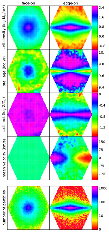
Figure 1: Spatially-resolved stellar properties of two simulated galaxies, D-MA_0 (face-on) on the left and D-MA_2 (edge-on) on the right. These maps show, from top to bottom, the stellar mass density, the mean luminosity-weighted ages and metallicities, the mean velocity along the line of sight, and the number of stellar particles in each spaxel (in logarithmic colour scale).

In addition, we also provide spatially-resolved measurements of the quantities listed in Table 6, considering the particles within each spaxel of our virtual CALIFA observations (see Section 4) for three different orientations.

• Stellar mass / surface density: total stellar mass within the spaxel and stellar surface density

• Star formation rate: calculated averaging the mass of stars formed in the last 100 Myr (Kennicutt, 1998)

• Stellar age / metallicity: mass- and luminosity-weighted means (1) and (2)

• Luminosity-weighted velocity (4) and velocity dispersion (3).

• Star formation histories: stellar mass formed within 100 Myr bins ordered in lookback time.

Some examples of these product datacubes (spatially resolved maps of intrinsic physical properties that are directly measured from the simulations) can be seen in Figure 1. They represent the final ‘solutions’ to be recovered from the mock observational data. Note that, for luminosity-weighted averages, we are adopting the usual definition of ‘intrinsic physical properties’ that ignores the effects of radiative transfer.

3 Spectral energy distribution

C-CS⁺

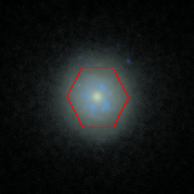
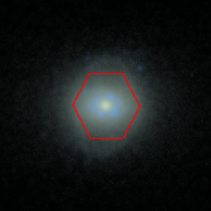
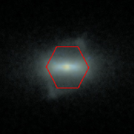
E-CS⁺

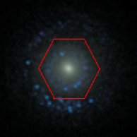
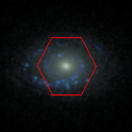
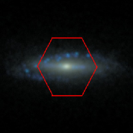
D-MA

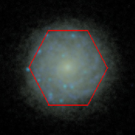
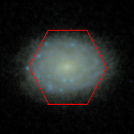
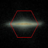
Figure 2: Composite synthetic broadband images created in the $(u,r,z)$-bands using the Lupton et al. (2004) composition algorithm for our three simulated galaxies (from top to bottom, C-CS⁺, E-CS⁺, and D-MA) in a field of view of $60\times 60$ kpc with $300\times 300$ pixels. The orientations are, from left to right, face-on, $45^{\circ}$ and edge-on, labelled in the synthetic datacubes as _0, _1 and _2 respectively. The red hexagon is the region of the simulations sampled by the CALIFA field of view, with physical sizes of $\sim 19,27,35$ kpc respectively for the C-CS⁺, E-CS⁺ and D-MA galaxies.

To generate the spatially-resolved spectral energy distribution of our simulated galaxies, we post-process the particles in the main halo in the simulations’ snapshots at redshift zero with the Monte Carlo radiative transfer code sunrise (Jonsson, 2006; Jonsson et al., 2010). sunrise is able to self-consistently compute the emission and propagation of light in a dusty InterStellar Medium (ISM). The resulting SEDs include the contribution of stellar and nebular emission, dust absorption and scattering, and hence show stellar absorption features, emission lines, as well as the effects of kinematics. More details about the sunrise input parameters used in this work can be found in Guidi et al. (2016).

In the first step, the code assigns a specific spectrum to each stellar particle depending on its age and metallicity, normalized to the mass of the particle. For ages $>10$ Myr, spectra from the starburst99 Stellar Population Synthesis (SPS) model (SB99, Leitherer et al. 1999) are assigned. They combine low-resolution stellar models ($\sim 20$-Å sampling) for wavelengths $\lambda<3000$ Å and $\lambda>7000$ Å, based on the Pauldrach/Hillier stellar atmospheres, while the high-resolution range ($3000-7000$ Å, with $0.3$-Å sampling) uses the fully theoretical atmospheres by Martins et al. (2005). On the other hand, young particles with age $\leq 10$ Myr are assigned a spectrum that takes into account the photo-dissociation and recombination of the gas, computed with the 1D photo-ionization code mappings III (Groves et al., 2004, 2008).

In the radiative transfer stage, $\sim 10^{7}$ randomly-generated photon packets are propagated through the dusty ISM with a Monte Carlo approach (with a constant dust-to-metals ratio of 0.4, Dwek 1998) assuming a Milky Way-like dust curve with $R_{V}=3.1$ (Cardelli et al., 1989; Draine, 2003). In the calculation of the kinematic broadening of the lines only the radial velocity of the particles is taken into account, neglecting both the velocity dispersion intrinsic in stellar clusters and the thermal broadening of the gas emission lines. This effect is certainly relevant for the intrinsic width of the emission lines, and in principle it could affect the detailed broadening of the stellar SED in those areas where few particles are present in a given spaxel (see bottom panel of Figure 1). Note that the sunrise kinematic algorithm consistently takes into account the Doppler shift when the light is scattered by dust, which can also modify the line profiles (Solf & Bohm, 1991; Henney, 1998; Grinin et al., 2012).

Finally, Monte Carlo photons are collected by cameras placed around the simulated galaxies to obtain the SED in each pixel. In our calculations we place cameras with three different orientations (defined according to the alignment of the total angular momentum of the stars with the $z$ direction) for each galaxy, respectively face-on, $45^{\circ}$ and edge-on (see Fig. 2 for the {$u,r,z$}-band colour-composite images). In order to reduce the random noise introduced by the sunrise Monte Carlo algorithm, the radiative transfer process described above is run ten times for each galaxy, changing only the random seeds, and the resulting spectra are averaged over the ten different random realizations. In this way we are able to reach a ‘signal-to-noise’ S/N (where N is the standard deviation over the ten realizations) of $\sim 300-400$ in the central spaxels and S/N$\sim 8-10$ in the outer regions, which is negligible compared to the typical values of the S/N in the CALIFA spectra that we aim to mimic (Sánchez et al., 2012a).

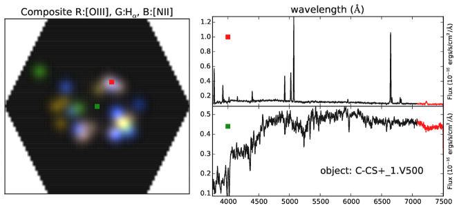
Figure 3: Left panel: RGB image of the [OIII]5007, H$\alpha$ and [NII]6584  emission lines for the galaxy C-CS⁺_1. Right panels: synthetic spectra in the spaxels corresponding to the red and green squares in the RGB image. In the upper right panel, the spaxel samples a nebular region (red square), while the lower right panel shows a V500 spectrum containing only stellar emission (green square). The part of the spectrum generated with the low-resolution stellar model (Sec. 3) is marked in red in the plot.

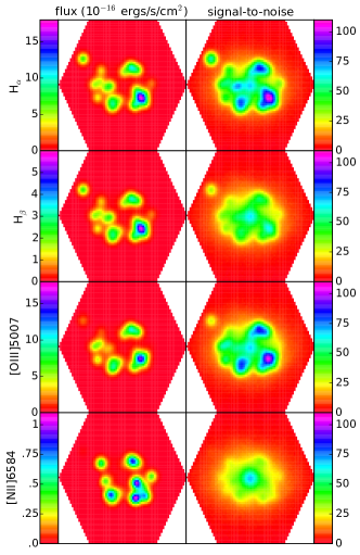
Figure 4: Line intensity (left) and Signal-to-Noise (right) maps of the four BPT lines (Baldwin et al., 1981) for the galaxy C-CS⁺_1. The S/N in every spaxel is obtained as the ratio between the mean signal and noise in the wavelength range of the corresponding emission line given in Table 8.

As part of the product datacubes, we provide the predicted SEDs of our galaxies, free from instrumental effects, as well as resolved maps of some spectral features derived from these theoretical datacubes. To obtain measurements of the properties of the stellar and nebular spectra without using any observational algorithm to separate the two spectral components (which may introduce many caveats and uncertainties), we additionally generate stellar-only synthetic datacubes following the same procedure described above, replacing the mappings spectra with starburst99 templates.

We generate the following maps:

• Lick indices: the strength of the Lick indices (Table 7 in Appendix A.2) is derived from the stellar-only datacubes, which have $2$-Å sampling.

• Nebular emission line intensities: the fluxes of different emission lines (Table 8) are measured after subtracting the stellar-only datacubes to the synthetic ones in order to take into account stellar absorption features in the calculation. Since the dust around young stars in the stellar-only datacubes is neglected, while is present at the sub-resolution level with mappings, for each line we renormalize the stellar-only spectra with the continuum level of the full cube at the lower bound of each line, and we compute the total flux between the lower and upper bounds of the lines after subtracting the continuum (the offsets between full and stellar-only cubes are indeed quite small, of the order $\sim 0.5-2\%$ of the flux). It is important to emphasize here that the nebular emission in the datacubes is limited to the stellar particles younger than 10 Myr (HII regions), and we do not count on any other sources of ionizing photons. The units are $10^{-16}$ erg s^-1 cm^-2 Å${}^{-1}~{}\text{spaxel}^{-1}$.

It should be noted that these quantities are measured from simulated spectra including the effects of dust and kinematics. Lick indices are defined over a short wavelength range, and therefore they are not expected to be strongly affected by dust extinction, although differential effects (highly dependent on the numerical resolution and assumed ISM physics of the simulations) may certainly play a role for realistic star formation histories (MacArthur, 2005). They also depend on the velocity dispersion at which they are measured (see e.g. Sánchez-Blázquez et al. 2006; Oliva-Altamirano et al. 2015). In IFS observational studies the spectra in each spaxel are usually broadened to a single velocity dispersion prior to the measurement of the Lick indices, in order to consistently compare them with models with the same dispersion (e.g. Wild et al., 2014). In our product datacubes we do not change the broadening of the absorption lines, since this procedure introduces additional uncertainties in the analysis. The spaxel-by-spaxel velocity dispersion is provided in the GALNAME.stellar.fits files (Sec. A.2) and can be used to tune the fitted models.

Our datacubes provide the nebular line intensities considering both the extinction within the nebula (implicit in the MAPPINGS templates) as well as absorption and scattering in the ISM (computed by sunrise). In Figure 3 we show an RGB image of the intensities (derived from the nebular maps) of the [OIII]5007, H_α and [NII]6584 emission lines, together with spectra in two different spaxels in the synthetic datacubes, one containing nebular emission and the other only stellar light. An example of these maps is given in Figure 4, where we show for one of our simulated galaxies the intensities of the BPT (Baldwin et al., 1981) emission lines (H_α, H_β, [OIII]5007, [NII]6584), and the corresponding signal-to-noise maps (see Section 4).

At variance with the intrinsic galaxy properties discussed in Section 2, we consider that Lick indices and nebular emission line intensities are properties of the SEDs, including the effects of geometry, kinematics, and radiative transport. These quantities (which may in principle be quite different from the sum of the intrinsic emissivities) are to be recovered from imperfect data, affected by the observational effects described below.

4 Mock observations

In this section we describe how we convert the output of the sunrise radiative transfer algorithm into synthetic IFS observations mimicking the CALIFA survey (Sánchez et al., 2012a; García-Benito et al., 2015). We briefly summarise the technical properties of the survey and explain how the main steps of the observation procedure are reproduced. A detailed description of the products that we make publicly available is provided in Appendix A.

Object	Redshift	Luminosity distance	Physical size
		[Mpc]	of the spaxels [kpc]
C-CS+	0.013	58.1	0.25
E-CS+	0.018	80.8	0.35
D-MA	0.024	108.2	0.45

Table 2: Redshift, luminosity distance and physical size covered by the spaxels in our synthetic CALIFA observations.

Setup	$N_{\alpha}$	$N_{\delta}$	$N_{\lambda}$	$\lambda$ (Å)	$d_{\lambda}$ (Å)	$\delta_{\lambda}$ (Å)	$\sigma_{0}$	$I_{0}$
V500	78	73	1877	$3749-7501$	2.0	6.0	0.29	20.8
V1200	78	73	1701	$3650-4840$	0.7	2.3	0.64	25.9

Table 3: Sizes of the simulated datacubes in the spatial and spectral dimensions ($N_{\alpha},N_{\delta},N_{\lambda}$), wavelength range, spectral sampling, and spectral resolution ($\lambda$, $d_{\lambda},\delta_{\lambda}$) of each instrumental setup, and best-fitting parameters ($\sigma_{0},I_{0}$) in equation (6) for the row-stacked spectra (RSS) of individual pointings in the CALIFA DR3.

CALIFA observations were taken with the Potsdam Multi-Aperture Spectrograph (PMAS, Roth et al., 2005), mounted on the Calar Alto 3.5-m telescope, utilizing the large hexagonal field of view offered by the PPak fibre bundle (Verheijen et al., 2004; Kelz et al., 2006). The final CALIFA Public Data Release (DR3, Sánchez et al. 2016a) consists of 667 galaxies. Sample selection (Walcher et al., 2014) and observing strategy (Sánchez et al., 2012a) aimed for a filling factor of 100% up to $\sim 2.5$ effective radii $R_{e}$. Datacubes have a field of view of $[76-78]^{\prime\prime}$ in right ascension and $[71-73]^{\prime\prime}$ in declination (depending on the observing conditions and the precise disposition of the dithering pattern for each object) sampled by $1^{\prime\prime}$ spaxels ($\sim 1$-kpc physical size). To reproduce these characteristics, we adopt a fixed $78^{\prime\prime}\times 73^{\prime\prime}$ configuration, we derive the half-light radius ($R_{50}$) in the $r$-band for every simulated galaxy, and then we adjust their redshift/distances (see Table 2) so that $78^{\prime\prime}$ correspond to $4\,{R_{50}}$.

The wavelength range, sampling, and resolution of the two spectral setups of the CALIFA survey (V500 and V1200; Sánchez et al., 2012a; García-Benito et al., 2015) are quoted in Table 3. Due to the implementation of stellar atmospheres in sunrise, (Section 3), we generate two radiative transfer simulations (one with high resolution and kinematics for $\lambda=3000-7000$ Å and another with low-resolution and no kinematics for $\lambda=7000-7600$ Å) for each galaxy. Then, we concatenate the SEDs at $\lambda=7000$ Å, apply the redshift of the object, and resample the spectra to the appropriate $d_{\lambda}$ for each setup. The regions of the V500 spectra generated with the low-resolution stellar model are flagged as bad pixels (see Section A.1), and they should not be used for SED fitting analysis.

These datacubes are convolved with a Gaussian kernel of $3.25^{\prime\prime}$ FWHM that adds in quadrature the response of the $3^{\prime\prime}$-diameter fibres of the PMAS/PPak instrument and an atmospheric seeing of $1.25^{\prime\prime}$, typical of a standard night at CALAR ALTO observatory. Then, they are ‘observed’ three times, positioning the 331 fibres of the instrument according to the dithering pattern followed in the CALIFA survey (Sánchez et al., 2007, 2012a), and the resulting $3\times 331=993$ row-stacked spectra (RSS) are convolved with another Gaussian that accounts for the spectral resolution $\delta_{\lambda}$ (Table 3) of each grating.

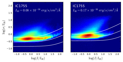
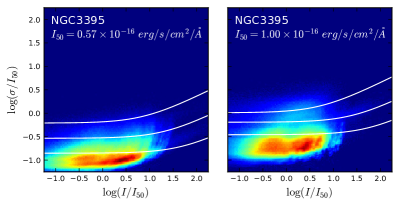
Figure 5: RSS noise characterization. Colour maps showing the distribution of the noise $\sigma$ relative to the signal $I$, normalized to the median value of the signal $I_{50}$ (in logarithmic scale) for two RSS datacubes. Left (right) panel displays the values corresponding to the V500 (V1200) setup. Middle white solid line shows the best-fit (median) curve for the $367\times 3$ CALIFA RSS. The fitting parameters ($\sigma_{0}$ and $I_{0}$) are given in Table 3. Solid white lines above and below represent the 90 and 10 percentiles of the parameter distribution. Colour scale corresponds to the number of pixels ($\sim 10^{7}$ in for every configuration).

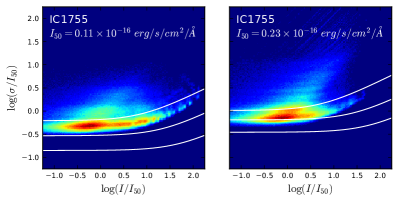
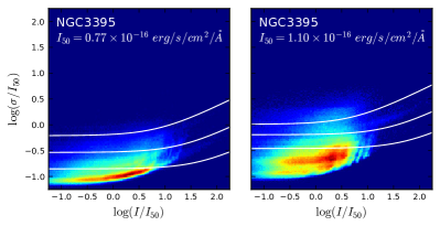
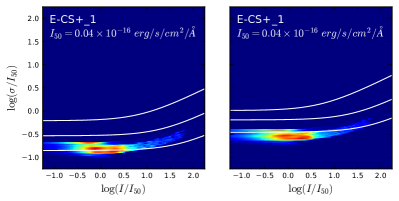
Figure 6: Datacube noise. The plot is identical to that of Figure 5. The upper two panels represent the noise distribution of the final datacubes corresponding to the two objects depicted in the previous figure. The lower panel corresponds to E-CS⁺_1, one of our synthetic datacubes. Our fit to the RSS data, prior to dithering and interpolation (same white lines as in Figure 5) is shown to guide the eye.

In order to account for detector noise, we selected galaxies from DR3 that were observed using both setups (V500 and V1200) and for which the quality flags indicate that the released cubes have only minor problems (see Section 6.4 of DR3). This sample consists of 367 galaxies out of the 667 forming the CALIFA DR3 (Sánchez et al., 2016a). We have analysed the raw-stacked spectra (RSS) corresponding to the three pointings of each object. The results show that the dependence of the noise with the intensity of the signal, characteristic of charge-coupled devices, can be modelled with a simple parametric formula

$$\sigma_{\rm n}=\sigma_{0}\sqrt{1+\frac{I_{\rm n}}{I_{0}}}$$ (6)

where $I_{\rm n}$ and $\sigma_{\rm n}$ refer to the observed intensity $I$ and errors $\sigma$ provided in the CALIFA datacubes normalized to the median value of the intensity, $\sigma_{\rm n}=\sigma/I_{50}$ and $I_{\rm n}=I/I_{50}$. The use of normalized errors and fluxes allows for a uniform object-independent unit-free characterization of the noise. Our analysis also reveals that the detector noise does not depend on wavelength, except for the expected edge effects.

We fit the free parameters of equation (6) to the data and then we take the median value of the results over the 367 objects considered. Best-fitting values are summarized in Table 3. The panels of Figure 5 show the relation between $\sigma_{\rm n}$ and $I_{\rm n}$ for two RSS datacubes selected from the CALIFA sample. These objects are chosen such as their fitted $\sigma_{0}$ and $I_{0}$ values lie below and above the 10 and 90 percentiles in the sample respectively (i.e. extreme cases). White solid lines represent, from top to bottom, the 90, 50 (median), and 10 percentiles. These average relations inferred from CALIFA RSS data are used to add random Gaussian noise and set the errors of our synthetic RSS files (three pointings per simulated galaxy and orientation) containing 331 spectra each.

In a final step, each set of three RSS files is combined into a single interpolated datacube using version V1.5 of the CALIFA pipeline (García-Benito et al., 2015), following exactly the same procedure as in real observations. Thus, our mock datacubes fully account for the effects of the dithering scheme, yielding a final PSF of $\sim 2.5^{\prime\prime}$ FWHM (Sánchez et al., 2012a) and introducing strong correlations between the noise of adjacent spaxels, as shown in Husemann et al. (2013); García-Benito et al. (2015) for real data. An example of the errors assigned by the CALIFA pipeline to the final datacubes and to one of our synthetic ones are plotted in Figure 6.

5 Science cases

Although the main aim of this manuscript is to describe the SELGIFS Data Challenge, and provide all the necessary details about the data set so that it can be meaningfully explored by the community, let us briefly illustrate here the kind of scientific questions that could be address by means of a toy example: the ability of different methods to recover the main physical properties of the stellar population.

A comparison based on observational data merely reflects the degree of agreement between different methods, but it is not possible to make an optimal choice, as the correct solution is not known, and the experiment offers limited insight about the reasons behind the observed discrepancies. The SELGIFS Data Challenge, on the other hand, provides an excellent benchmark to obtain more robust conclusions, but a significant amount of time and effort would be necessary. Let us consider, for instance, the stellar mass, as well as the mass-weighted and luminosity-weighted stellar ages and metallicities, recovered by the following methods:

• Steckmap – PSB (Ocvirk et al., 2006a, b).

• Pipe3D – SFS (Sánchez et al., 2016b, c).

• Starlight – LG (Cid Fernandes et al., 2005; Cid Fernandes et al., 2013), with the same setup as Galbany et al. (2014, 2016b).

• Starlight – RGB (setup as in García-Benito et al., 2017, including Salpeter IMF).

The reader is referred to the aforementioned publications for a thorough description of each algorithm and the adopted parameter settings. Here, the default choices adopted by some of the authors of the present manuscript have been used in order to provide a rough indication of the expected size of the uncertainties, but the results of this naive exercise only stress the need for much more extensive studies that rigorously explore the origin of the systematic uncertainties in each individual quantity for every different method and parameter configuration.

In essence, all the methods considered decompose the observed spectrum as a sum of simple stellar populations (SSPs) with different ages and metallicities and a set of nebular emission lines. The average stellar properties are then estimated from the coefficients assigned to each SSP. We compare the outputs of these methods, run on our simulated V500-like datacubes, with the true solution given by the product datacubes (convolved with the PSF) for two of our simulated galaxies (C-CS⁺_1 and D-MA_0). Results for the stellar mass, age, and metallicity are plotted in Figures 7, 8, and 9, respectively. For each quantity, we plot colour maps of the relative accuracy

$$\delta_{i}=\log_{10}(Q_{i}-Q_{0})$$ (7)

expressed in dex, where $Q_{i}$ denotes the value returned by each method and $Q_{0}$ represents the solution to be recovered. The mass-weighted average

$$\langle\delta_{i}\rangle_{M}=\frac{\sum\mu_{*}(x,y)\ \delta_{i}(x,y)}{\sum\mu_{*}(x,y)}$$ (8)

and standard deviation

$$\sqrt{\langle\delta_{i}^{2}\rangle_{M}-\langle\delta_{i}\rangle_{M}^{2}}$$ (9)

of the relative accuracy for each quantity, method, and galaxy are quoted in Table 4, where $\mu_{*}(x,y)$ denotes the local stellar surface density at each spaxel.

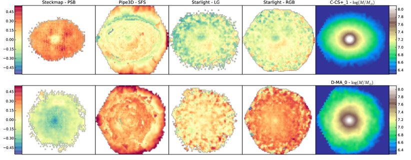
Figure 7: Relative accuracy (measured in dex) of the stellar mass distribution recovered by different codes, compared to the true solution (shown in the rightmost column) for simulated galaxies C-CS⁺_1 (top) and D-MA_0 (bottom).

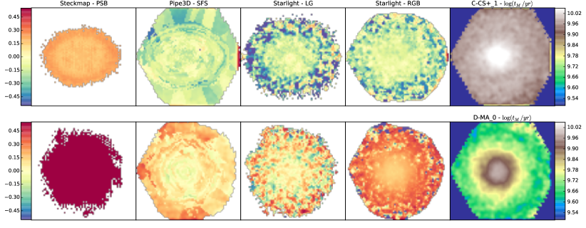
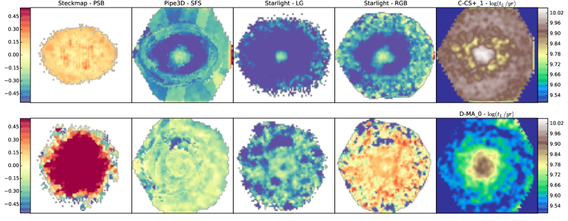
Figure 8: Same as Figure 7, for the mass-weighted (first two rows) and luminosity-weighted (last two rows) stellar age.

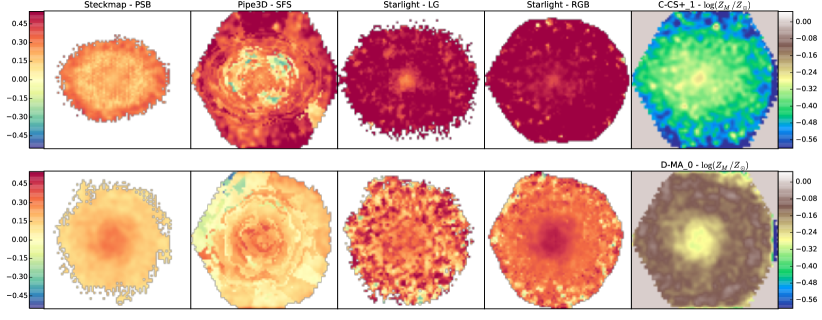
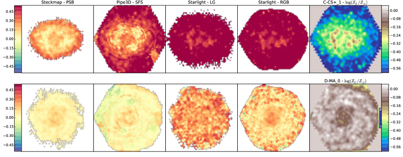
Figure 9: Same as Figure 7, for the mass-weighted (first two rows) and luminosity-weighted (last two rows) stellar metallicities.

Galaxy	Method	mass	$\langle$ age $\rangle_{M}$	$\langle$ age $\rangle_{L}$	$\langle Z\rangle_{M}$	$\langle Z\rangle_{L}$
	Steckmap – PSB	$~{}~{}0.249\pm 0.071$	$~{}~{}0.207\pm 0.031$	$~{}~{}0.132\pm 0.047$	$~{}~{}0.253\pm 0.066$	$~{}~{}0.208\pm 0.106$
C-CS+_1	Pipe3D – SFS	$~{}~{}0.047\pm 0.179$	$-0.139\pm 0.144$	$-0.406\pm 0.192$	$~{}~{}0.375\pm 0.205$	$~{}~{}0.438\pm 0.206$
	Starlight – LG	$-0.126\pm 0.119$	$-0.237\pm 0.210$	$-0.717\pm 0.279$	$~{}~{}0.608\pm 0.142$	$~{}~{}0.696\pm 0.158$
	Starlight – RGB	$-0.059\pm 0.105$	$-0.163\pm 0.150$	$-0.448\pm 0.204$	$~{}~{}0.605\pm 0.109$	$~{}~{}0.657\pm 0.133$
	Steckmap – PSB	$-0.140\pm 0.083$	$~{}~{}7.043\pm 0.411$	$~{}~{}0.732\pm 0.841$	$~{}~{}0.166\pm 0.048$	$~{}~{}0.051\pm 0.036$
D-MA_0	Pipe3D – SFS	$~{}~{}0.242\pm 0.140$	$~{}~{}0.107\pm 0.102$	$-0.185\pm 0.099$	$~{}~{}0.126\pm 0.110$	$~{}~{}0.021\pm 0.080$
	Starlight – LG	$~{}~{}0.086\pm 0.115$	$~{}~{}0.043\pm 0.197$	$-0.418\pm 0.224$	$~{}~{}0.310\pm 0.137$	$~{}~{}0.238\pm 0.105$
	Starlight – RGB	$~{}~{}0.248\pm 0.135$	$~{}~{}0.205\pm 0.272$	$-0.043\pm 0.405$	$~{}~{}0.326\pm 0.099$	$~{}~{}0.138\pm 0.113$

Table 4: Mass-weighted mean and standard deviation of the relative accuracy of each method (measured in dex) for the quantities displayed in Figures 7, 8, and 9.

The interpretation of these results is anything but straightforward. With a few exceptions, all methods are able to recover the true solution within a factor of two (0.3 dex). However, the relative accuracy depends on the quantity and method in an intricate way, that seems to be different for different galaxies. Finding the causes of such behaviour (e.g. choice of IMF, SSP basis, fitting method, precise definition of the averaging procedure, dust extinction prescription, physical properties of the galaxy, etc.), especially in the catastrophic cases, requires a thorough analysis that is beyond the scope of the present work.

These results emphasise the influence on the adopted methodology and parameters on the recovered physical properties of the galaxies. However, none of the prescriptions considered here can be singled out as better or worse than the others. Even in this simple test, with very limited coverage of the huge parameter space (both on the simulation and the analysis side), it is difficult to identify clear systematic trends. Some codes, with certain settings, are able to recover some parameters more accurately than others in one galaxy, but fare worse on another.

We argue that using any of the methods available in the literature with default parameter settings will probably incur in systematic uncertainties that are much larger than the reported statistical errors. Understanding the effects of each parameter in detail is required in order to estimate the magnitude of the systematic uncertainty in a realistic case. The SELGIFS Data Challenge can be extremely useful in this respect, and we encourage the reader to experiment with it. Let us please warn, nevertheless, that the data set is not meant as a test bed to optimise the parameter settings of any given algorithm. This would only guarantee the optimal recovery of our simulated conditions, which may not bear any close relation to reality whatsoever.

6 Summary

We use hydrodynamical simulations of galaxies formed in a cosmological context to generate mock data mimicking the Integral Field Spectroscopy (IFS) survey CALIFA (Sánchez et al., 2012a). The hydrodynamical code follows, in addition to gravity and hydrodynamics, many other relevant galactic-scale physical processes, such as energy feedback and chemical enrichment from SNe explosions, multi-phase InterStellar Medium (ISM), and metal-dependent cooling of the gas. Our hydrodynamical simulations have been post-processed with the radiative transfer code sunrise, in order to obtain their spatially-resolved spectral energy distributions. These spectra contain the light emitted by the stars and the nebulae (young stars) in the simulations, and include the broadening of the absorption and emission lines due to kinematics, as well as the extinction and scattering by the dust in the ISM.

The input parameters in sunrise have been tuned to reproduce the properties of the CALIFA instrument in terms of field of view size, number of spaxels and spectral range. After we obtain the results of the radiative transfer with sunrise, we redshift the simulated spectra to match the physical size covered by the spaxels in the radiative transfer stage with the angular resolution of the PMAS instrument used in CALIFA, and we resample and cut these spectra according to the sampling and wavelength range of the low-resolution V500 and blue mid-resolution V1200 CALIFA setups. We convert our spatially-resolved spectra into the V500 and V1200 data format of the CALIFA DR2, and we convolve these 3-dimensional datasets with Gaussian Point Spread Functions both in the spatial and spectral dimensions, mimicking the properties of the CALIFA observations in terms of spatial and spectral resolution. Finally, after we parametrize the properties of the noise in a sample of 367 galaxies both from the CALIFA V500 and V1200 datasets, we add similar noise to the simulated V500 and V1200 data.

Our final sample of 18 datacubes (3 objects with 3 inclinations both in the V500 and V1200 setups) provide observers with a powerful benchmark to test the accuracy and calibration of their analysis tools and set the basis for a reliable comparison between simulations and IFS observational data. To this purpose we generate, together with the synthetic IFS observations, a corresponding set of product datacubes, i.e. resolved maps of several properties computed directly from the simulations and/or simulated noiseless datacubes.

Although this work is specifically designed to reproduce the properties of the CALIFA observations, the method illustrated in this paper can be easily extended to mimic other integral field spectrographs such as MUSE (Bacon et al., 2004), WEAVE (Dalton et al., 2014), MaNGA (Bundy et al., 2015) or SAMI (Allen et al., 2015) by changing some of the input parameters in the radiative transfer stage and performing a similar study of the detector noise. Hence, this procedure can be easily applied to generate synthetic observations for different IFS instruments, or for studying a specific science case prior to applying for observing time. The present project can also be extended to use other hydrodynamical simulations, which will be very important in order to enlarge the given dataset and consider a more complete sample of galaxies in terms of morphology, total mass, stellar age and metallicity, gas content and merger history.

We then encourage researchers to contact the authors in case they are interested in obtaining simulated data mimicking the properties of different IFS surveys, or if they have interest in converting their hydrodynamical simulations into CALIFA-like datacubes. We hope that this work would promote more collaboration and connection among observers and simulators, as this will be of crucial importance in view of the several ongoing and future IFS surveys, which will provide the community with large datasets of spatially-resolved properties of galaxies at different cosmic times, allowing to study galaxy formation physics at a higher level of detail than ever before.

Appendix A The SELGIFS data challenge

The main goal of this work is to provide the scientific community with a reliable set of synthetic IFS observations, and with the corresponding maps of directly measured properties, that allows to test existing (and future) dedicated analysis tools, as well as to create a benchmark for verifying hypothesis and/or preparing observations.

The data are distributed through a web page hosted by the Universidad Autónoma de Madrid. The description of the different files and their data format is presented in the following sections.

A.1 Synthetic observations

HDU	Extension name	Format	Content
0	PRIMARY	32-bit float	flux density in $10^{-16}$ erg s-1 cm-2 Å-1
1	ERROR	32-bit float	$1\sigma$ error on the flux density
2	ERRWEIGHT	32-bit float	error weighting factor
3	BADPIX	8-bit integer	bad pixel flags (1=bad, 0=good)
4	FIBCOVER	8-bit integer	number of fibres used to fill each spaxel

Table 5: Structure of the CALIFA FITS files in DR2 (from García-Benito et al. 2015).

Our synthetic CALIFA datacubes in the two V500 and V1200 setups (Section 4) are provided in different files, identified following the CALIFA DR2 naming convention GALNAME.V500.cube.fits.gz and GALNAME.V1200.cube.fits.gz for the V500 and V1200 respectively. The data structure of these simulated data closely follows the one adopted in CALIFA, namely datacubes in the standard FITS file format.

The FITS header of the simulated datacubes stores only the most relevant keywords available in the DR2 header. Most of the DR2 keywords containing information about the pointing, the reduction pipeline, Galactic extinction, sky brightness, etc. have been removed. The flux unit has been stored under the keyword PIPE UNITS as in the CALIFA datacubes.

Each FITS file contains the data for a single galaxy stored in five HDU (see Table 5), every one of them providing different information according to the data format of the pipeline V1.5 used in DR2 (García-Benito et al., 2015). The first two axes in the datacubes ($N_{\alpha}$, $N_{\delta}$) correspond to the spatial dimensions (along the right ascension and declination) with a $1"\times 1"$ sampling. The third dimension ($N_{\lambda}$) represents the wavelength axis, with ranges and samplings described in Section 4 and Table 3.

Here we summarize the content of each HDU:

0) Primary (PRIMARY)

The primary HDU contains the measured flux densities in CALIFA units of $10^{-16}$ erg s^-1 cm^-2 Å^-1.

1) Error (ERROR)

This extension provides the values of the $1\sigma$ noise level in each pixel, calculated according to Eq. 6. In the case of bad pixels, we store a value of $10^{10}$ following the CALIFA data structure.

2) Error weight (ERRWEIGHT)

This HDU gives the error scaling factor for each pixel, in the case that all valid pixels of the cubes are co-added (see appendix A of García-Benito et al. 2015).

3) Bad pixel (BADPIX)

This extension stores a flag advising on potential problems in a pixel; in the CALIFA dataset this may occur for instance due to cosmic rays contamination, bad CCD columns, or the effect of vignetting. In our datacubes we flag as bad pixel (i.e. equal to 1) the regions in the spectra that are generated with the lower-resolution stellar model (see Section 3).

4) fibre coverage (FIBCOVER)

This HDU, available only from DR2, accounts for the number of fibers used to recover the flux (see section 4.3 of García-Benito et al. 2015).

In addition to these datacubes, we provide in the following files synthetic data free of any observational effect, in the same data format and physical units.

• GALNAME.SED.fits: it contains the simulated SEDs prior to the addition of the observational effects (noise and PSFs, see sec. 4). The spatially-resolved SEDs are stored in a single HDU with $78\times 73$ pixels in the spatial dimensions and 1877 pixels in the wavelength dimension, with 2 Å  sampling following the V500 data format (tab. 3).

Stellar property	Units
Mass	$\log(\text{M}_{\odot})$
Mass density	$\log(\text{M}_{\odot}/\text{pc}^{2})$
Mean age mass-weighted	$\log(\text{yr})$
Mean metallicity mass-weighted	$\log(\text{Z}/\text{Z}_{\odot})$
Mean age luminosity-weighted	$\log(\text{yr})$
Mean metallicity luminosity-weighted	$\log(\text{Z}/\text{Z}_{\odot})$
Mean velocity	km/s
Velocity dispersion	km/s
Star formation rate	M⊙/yr
Stellar particles number	–

Table 6: List of the spatially-resolved stellar properties provided in the product datacubes.

Name	Index Bandpass (Å)	Blue continuum bandpass (Å)	Red continuum bandpass (Å)	Units	Reference
CN1	4142.125 - 4177.125	4080.125 - 4117.625	4244.125 - 4284.125	mag	Worthey et al. (1994)
CN2	4142.125 - 4177.125	4083.875 - 4096.375	4244.125 - 4284.125	mag	Worthey et al. (1994)
Ca4227	4222.250 - 4234.750	4211.000 - 4219.750	4241.000 - 4251.000	Å	Worthey et al. (1994)
G4300	4281.375 - 4316.375	4266.375 - 4282.625	4318.875 - 4335.125	Å	Worthey et al. (1994)
Fe4383	4369.125 - 4420.375	4359.125 - 4370.375	4442.875 - 4455.375	Å	Worthey et al. (1994)
Ca4455	4452.125 - 4474.625	4445.875 - 4454.625	4477.125 - 4492.125	Å	Worthey et al. (1994)
Fe4531	4514.250 - 4559.250	4504.250 - 4514.250	4560.500 - 4579.250	Å	Worthey et al. (1994)
Fe4668	4634.000 - 4720.250	4611.500 - 4630.250	4742.750 - 4756.500	Å	Worthey et al. (1994)
H$\beta$	4847.875 - 4876.625	4827.875 - 4847.875	4876.625 - 4891.625	Å	Worthey et al. (1994)
Fe5015	4977.750 - 5054.000	4946.500 - 4977.750	5054.000 - 5065.250	Å	Worthey et al. (1994)
Mg1	5069.125 - 5134.125	4895.125 - 4957.625	5301.125 - 5366.125	mag	Worthey et al. (1994)
Mg2	5154.125 - 5196.625	4895.125 - 4957.625	5301.125 - 5366.125	mag	Worthey et al. (1994)
Mg$b$	5160.125 - 5192.625	5142.625 - 5161.375	5191.375 - 5206.375	Å	Worthey et al. (1994)
Fe5270	5245.650 - 5285.650	5233.150 - 5248.150	5285.650 - 5318.150	Å	Worthey et al. (1994)
Fe5335	5312.125 - 5352.125	5304.625 - 5315.875	5353.375 - 5363.375	Å	Worthey et al. (1994)
Fe5406	5387.500 - 5415.000	5376.250 - 5387.500	5415.000 - 5425.000	Å	Worthey et al. (1994)
Fe5709	5696.625 - 5720.375	5672.875 - 5696.625	5722.875 - 5736.625	Å	Worthey et al. (1994)
Fe5782	5776.625 - 5796.625	5765.375 - 5775.375	5797.875 - 5811.625	Å	Worthey et al. (1994)
Na D	5876.875 - 5909.375	5860.625 - 5875.625	5922.125 - 5948.125	Å	Worthey et al. (1994)
TiO1	5936.625 - 5994.125	5816.625 - 5849.125	6038.625 - 6103.625	mag	Worthey et al. (1994)
TiO2	6189.625 - 6272.125	6066.625 - 6141.625	6372.625 - 6415.125	mag	Worthey et al. (1994)
H$\delta_{A}$	4083.500 - 4122.250	4041.600 - 4079.750	4128.500 - 4161.000	Å	Worthey & Ottaviani (1997)
H$\gamma_{A}$	4319.750 - 4363.500	4283.500 - 4319.750	4367.250 - 4419.750	Å	Worthey & Ottaviani (1997)
H$\delta_{F}$	4091.000 - 4112.250	4057.250 - 4088.500	4114.750 - 4137.250	Å	Worthey & Ottaviani (1997)
H$\gamma_{F}$	4331.250 - 4352.250	4283.500 - 4319.750	4354.750 - 4384.750	Å	Worthey & Ottaviani (1997)
D4000_n		3850.000 - 3950.000	4000.000 - 4100.000		Balogh et al. (1999)

Table 7: List of the absorption line indices for which the strength in each spaxel is provided, together with the definition of the continuum and bandpass wavelength ranges.

Species	Line centre (Å)	Lower/
		upper bounds (Å)
[Ne III]3869	3869.060	$3859-3879$
H$\delta$	4101.734	$4092-4111$
H$\gamma$	4340.464	$4330-4350$
[O III]4363	4363.210	$4350-4378$
H$\beta$	4861.325	$4851-4871$
[O III]4959	4958.911	$4949-4969$
[O III]5007	5006.843	$4997-5017$
HeI 5876	5875.670	$5866-5886$
[N II]6548	6548.040	$6533-6553$
H$\alpha$	6562.800	$6553-6573$
[N II]6584	6583.460	$6573-6593$
[S II]6717	6716.440	$6704-6724$
[S II]6731	6730.810	$6724-6744$

Table 8: List of the emission line intensities provided in the product datacubes. Line centers, lower and upper bounds are taken from the Sloan Digital Sky Survey-Garching DR7 analysis (available at the url http://wwwmpa.mpa-garching.mpg.de/SDSS/DR7/).

A.2 Product datacubes

The direct calculation of the resolved (spaxel-by-spaxel) galaxy properties described in Sections 2 and 3 are provided in separate files. These maps have been calculated directly from the simulations’ output, or from the noiseless synthetic spectra prior to the addition of any observational effect.

The name of the files and data format are listed below:

• GALNAME.stellar.fits: the file contains the resolved maps obtained directly from the hydrodynamical simulations as described in Section 2. These FITS files have a single Header Data Unit (HDU) holding a 10-layer matrix, containing the nine $78\times 73$ maps of the stellar properties in the order given in Table 6. The header includes the information about the physical property stored in every layer (DESC_*) and its units (UNITS_*), where * refers to the layer number.

• GALNAME.SFH.fits: it provides the resolved SFHs, storing the mass (in solar units) formed in bins of 100 Myr. It contains a single HDU with a $78\times 73\times 140$ array. The 140 time bins are ordered in lookback time, with the first element storing the mass formed in the last 100 Myr.

• GALNAME.Lick_indices.fits: this file stores the resolved maps for the 26 Lick indices measured from the noiseless stellar-only datacube (see Section 3). Each file consists of a single HDU unit with a 26-layer matrix that contains the twenty-five $78\times 73$ maps of the different absorption features listed in Table 7. The header provides for each layer the Lick index name (DESC_*) and its measured units (UNITS_*), with * indicating the layer number.

• GALNAME.nebular.fits: it encloses the resolved maps for the 13 nebular line intensities measured from the noiseless nebular-only datacube (Sec. 3). The data are stored in a single HDU unit with a 13-layer matrix, containing all the thirteen $78\times 73$ maps of the nebular lines given in Table 8. The header stores the line names (DESC_*), rest frame wavelengths (LAMBDA_*) and units (UNITS_*) for each layer * in the file.

In order to provide results directly comparable with the ones generated by the observational algorithms applied to the synthetic datacubes, maps at the same spatial resolution of the synthetic datacubes are additionally available. These have been obtained convolving the stellar maps with a 2.5 FWHM Gaussian kernel, and the synthetic spectra with a 2.5” FWHM PSF before extracting the Lick indices and the nebular line intensities as described in Section 3. Notice that when we compute the logarithmic quantities in the stellar maps the PSF is added prior to the calculation of the logarithm.

References

- Abazajian et al. (2009) Abazajian K. N., et al., 2009, ApJS, 182, 543
- Allen et al. (2015) Allen J. T., Croom S. M., Konstantopoulos I. S., Bryant J. J., Sharp R., et al. 2015, MNRAS, 446, 1567
- Asari et al. (2007) Asari N. V., Cid Fernandes R., Stasińska G., Torres-Papaqui J. P., Mateus A., Sodré L., Schoenell W., Gomes J. M., 2007, MNRAS, 381, 263
- Aumer et al. (2013) Aumer M., White S. D. M., Naab T., Scannapieco C., 2013, MNRAS, 434, 3142
- Bacon et al. (2001) Bacon R., et al., 2001, MNRAS, 326, 23
- Bacon et al. (2004) Bacon R., Bauer S.-M., Bower R., Cabrit S., Cappellari M., Carollo M., et al. 2004, in Moorwood A. F. M., Iye M., eds, Society of Photo-Optical Instrumentation Engineers (SPIE) Conference Series Vol. 5492, Ground-based Instrumentation for Astronomy. pp 1145–1149, doi:10.1117/12.549009
- Baldwin et al. (1981) Baldwin J. A., Phillips M. M., Terlevich R., 1981, PASP, 93, 5
- Balogh et al. (1999) Balogh M. L., Morris S. L., Yee H. K. C., Carlberg R. G., Ellingson E., 1999, ApJ, 527, 54
- Bellovary et al. (2014) Bellovary J. M., Holley-Bockelmann K., Gültekin K., Christensen C. R., Governato F., Brooks A. M., Loebman S., Munshi F., 2014, MNRAS, 445, 2667
- Bershady et al. (2010) Bershady M. A., Verheijen M. A. W., Swaters R. A., Andersen D. R., Westfall K. B., Martinsson T., 2010, ApJ, 716, 198
- Bertin & Arnouts (1996) Bertin E., Arnouts S., 1996, A&AS, 117, 393
- Birkmann et al. (2010) Birkmann S. M., et al., 2010, in Space Telescopes and Instrumentation 2010: Optical, Infrared, and Millimeter Wave. p. 77310D, doi:10.1117/12.858000
- Bundy et al. (2015) Bundy K., Bershady M. A., Law D. R., Yan R., Drory N., MacDonald N., et al. 2015, ApJ, 798, 7
- Cappellari & Copin (2003) Cappellari M., Copin Y., 2003, MNRAS, 342, 345
- Cappellari & Emsellem (2004) Cappellari M., Emsellem E., 2004, PASP, 116, 138
- Cappellari et al. (2011) Cappellari M., et al., 2011, MNRAS, 413, 813
- Cardelli et al. (1989) Cardelli J. A., Clayton G. C., Mathis J. S., 1989, ApJ, 345, 245
- Casado et al. (2016) Casado J., Ascasibar Y., García-Benito R., Guidi G., Choudhury O. S., Bellocchi E., Sánchez S., Díaz A. I., 2016, ArXiv:1607.07299,
- Chieffi & Limongi (2004) Chieffi A., Limongi M., 2004, ApJ, 608, 405
- Cid Fernandes et al. (2005) Cid Fernandes R., Mateus A., Sodré L., Stasińska G., Gomes J. M., 2005, MNRAS, 358, 363
- Cid Fernandes et al. (2013) Cid Fernandes R., et al., 2013, A&A, 557, A86
- Croom et al. (2012) Croom S. M., et al., 2012, MNRAS, 421, 872
- Dalton et al. (2014) Dalton G., Trager S., Abrams D. C., Bonifacio P., López Aguerri J. A., et al. 2014, in Society of Photo-Optical Instrumentation Engineers (SPIE) Conference Series. p. 0 (arXiv:1412.0843), doi:10.1117/12.2055132
- Diehl & Statler (2006) Diehl S., Statler T. S., 2006, MNRAS, 368, 497
- Draine (2003) Draine B. T., 2003, ApJ, 598, 1017
- Dwek (1998) Dwek E., 1998, ApJ, 501, 643
- Förster Schreiber et al. (2009) Förster Schreiber N. M., et al., 2009, ApJ, 706, 1364
- Galbany et al. (2014) Galbany L., et al., 2014, A&A, 572, A38
- Galbany et al. (2016a) Galbany L., et al., 2016a, MNRAS, 455, 4087
- Galbany et al. (2016b) Galbany L., et al., 2016b, A&A, 591, A48
- Gallazzi et al. (2005) Gallazzi A., Charlot S., Brinchmann J., White S. D. M., Tremonti C. A., 2005, MNRAS, 362, 41
- García-Benito et al. (2015) García-Benito R., et al., 2015, A&A, 576, A135
- García-Benito et al. (2017) García-Benito R., et al., 2017, preprint, (arXiv:1709.00413)
- González Delgado et al. (2014) González Delgado R. M., et al., 2014, A&A, 562, A47
- González Delgado et al. (2015) González Delgado R. M., et al., 2015, A&A, 581, A103
- Governato et al. (2007) Governato F., Willman B., Mayer L., Brooks A., Stinson G., Valenzuela O., Wadsley J., Quinn T., 2007, MNRAS, 374, 1479
- Governato et al. (2010) Governato F., et al., 2010, Nature, 463, 203
- Grinin et al. (2012) Grinin V. P., Tambovtseva L. V., Weigelt G., 2012, A&A, 544, A45
- Groves et al. (2004) Groves B. A., Dopita M. A., Sutherland R. S., 2004, ApJS, 153, 9
- Groves et al. (2008) Groves B., Dopita M. A., Sutherland R. S., Kewley L. J., Fischera J., Leitherer C., Brandl B., van Breugel W., 2008, ApJS, 176, 438
- Guidi et al. (2015) Guidi G., Scannapieco C., Walcher C. J., 2015, MNRAS, 454, 2381
- Guidi et al. (2016) Guidi G., Scannapieco C., Walcher J., Gallazzi A., 2016, MNRAS, 462, 2046
- Hayward & Smith (2015) Hayward C. C., Smith D. J. B., 2015, MNRAS, 446, 1512
- Hayward et al. (2014) Hayward C. C., et al., 2014, MNRAS, 445, 1598
- Henney (1998) Henney W. J., 1998, ApJ, 503, 760
- Husemann et al. (2013) Husemann B., Jahnke K., Sánchez S. F. e. a., 2013, A&A, 549, A87
- Jonsson (2006) Jonsson P., 2006, MNRAS, 372, 2
- Jonsson et al. (2010) Jonsson P., Groves B. A., Cox T. J., 2010, MNRAS, 403, 17
- Karakas (2010) Karakas A. I., 2010, MNRAS, 403, 1413
- Kelz et al. (2006) Kelz A., et al., 2006, PASP, 118, 129
- Kendrew et al. (2016) Kendrew S., et al., 2016, MNRAS, 458, 2405
- Kennicutt (1998) Kennicutt Jr. R. C., 1998, ARA&A, 36, 189
- Koleva et al. (2009) Koleva M., Prugniel P., Bouchard A., Wu Y., 2009, A&A, 501, 1269
- Leitherer et al. (1999) Leitherer C., et al., 1999, ApJS, 123, 3
- Lupton et al. (2004) Lupton R., Blanton M. R., Fekete G., Hogg D. W., O’Mullane W., Szalay A., Wherry N., 2004, PASP, 116, 133
- MacArthur (2005) MacArthur L. A., 2005, ApJ, 623, 795
- MacArthur et al. (2009) MacArthur L. A., González J. J., Courteau S., 2009, MNRAS, 395, 28
- Marigo (2001) Marigo P., 2001, A&A, 370, 194
- Martins et al. (2005) Martins L. P., González Delgado R. M., Leitherer C., Cerviño M., Hauschildt P., 2005, MNRAS, 358, 49
- Michałowski et al. (2014) Michałowski M. J., Hayward C. C., Dunlop J. S., Bruce V. A., Cirasuolo M., Cullen F., Hernquist L., 2014, A&A, 571, A75
- Nelson et al. (2015) Nelson D., et al., 2015, Astronomy and Computing, 13, 12
- Ocvirk et al. (2006a) Ocvirk P., Pichon C., Lançon A., Thiébaut E., 2006a, MNRAS, 365, 46
- Ocvirk et al. (2006b) Ocvirk P., Pichon C., Lançon A., Thiébaut E., 2006b, MNRAS, 365, 74
- Oliva-Altamirano et al. (2015) Oliva-Altamirano P., Brough S., Jimmy Kim-Vy T., Couch W. J., McDermid R. M., Lidman C., von der Linden A., Sharp R., 2015, MNRAS, 449, 3347
- Papaderos et al. (2002) Papaderos P., Izotov Y. I., Thuan T. X., Noeske K. G., Fricke K. J., Guseva N. G., Green R. F., 2002, A&A, 393, 461
- Portinari et al. (1998) Portinari L., Chiosi C., Bressan A., 1998, A&A, 334, 505
- Rosales-Ortega et al. (2010) Rosales-Ortega F. F., Kennicutt R. C., Sánchez S. F., Díaz A. I., Pasquali A., Johnson B. D., Hao C. N., 2010, MNRAS, 405, 735
- Roth et al. (2005) Roth M. M., et al., 2005, PASP, 117, 620
- Ruiz-Lara et al. (2016) Ruiz-Lara T., et al., 2016, MNRAS, 456, L35
- Sánchez-Blázquez et al. (2006) Sánchez-Blázquez P., Gorgas J., Cardiel N., González J. J., 2006, A&A, 457, 787
- Sánchez et al. (2007) Sánchez S. F., Cardiel N., Verheijen M. A. W., Martín-Gordón D., Vilchez J. M., Alves J., 2007, A&A, 465, 207
- Sánchez et al. (2012a) Sánchez S. F., et al., 2012a, A&A, 538, A8
- Sánchez et al. (2012b) Sánchez S. F., et al., 2012b, A&A, 546, A2
- Sánchez et al. (2016a) Sánchez S. F., et al., 2016a, ArXiv:1604.02289,
- Sánchez et al. (2016b) Sánchez S. F., et al., 2016b, Rev. Mexicana Astron. Astrofis., 52, 21
- Sánchez et al. (2016c) Sánchez S. F., et al., 2016c, Rev. Mexicana Astron. Astrofis., 52, 171
- Sanders & Fabian (2001) Sanders J. S., Fabian A. C., 2001, MNRAS, 325, 178
- Sarzi et al. (2006) Sarzi M., et al., 2006, MNRAS, 366, 1151
- Scannapieco et al. (2005) Scannapieco C., Tissera P. B., White S. D. M., Springel V., 2005, MNRAS, 364, 552
- Scannapieco et al. (2006) Scannapieco C., Tissera P. B., White S. D. M., Springel V., 2006, MNRAS, 371, 1125
- Scannapieco et al. (2008) Scannapieco C., Tissera P. B., White S. D. M., Springel V., 2008, MNRAS, 389, 1137
- Scannapieco et al. (2009) Scannapieco C., White S. D. M., Springel V., Tissera P. B., 2009, MNRAS, 396, 696 (S09)
- Scannapieco et al. (2010) Scannapieco C., Gadotti D. A., Jonsson P., White S. D. M., 2010, MNRAS, 407, L41
- Scannapieco et al. (2012) Scannapieco C., et al., 2012, MNRAS, 423, 1726
- Schaye et al. (2015) Schaye J., Crain R. A., Bower R. G., Furlong M., et al. 2015, MNRAS, 446, 521
- Smith & Hayward (2015) Smith D. J. B., Hayward C. C., 2015, MNRAS, 453, 1597
- Solf & Bohm (1991) Solf J., Bohm K. H., 1991, ApJ, 375, 618
- Springel (2005) Springel V., 2005, MNRAS, 364, 1105
- Springel & Hernquist (2003) Springel V., Hernquist L., 2003, MNRAS, 339, 289
- Springel et al. (2008) Springel V., et al., 2008, MNRAS, 391, 1685
- Stetson (1987) Stetson P. B., 1987, PASP, 99, 191
- Stott et al. (2016) Stott J. P., et al., 2016, MNRAS, 457, 1888
- Sutherland & Dopita (1993) Sutherland R. S., Dopita M. A., 1993, ApJS, 88, 253
- Thatte et al. (2014) Thatte N. A., et al., 2014, in Ground-based and Airborne Instrumentation for Astronomy V. p. 914725, doi:10.1117/12.2055436
- Tormen et al. (1997) Tormen G., Bouchet F. R., White S. D. M., 1997, MNRAS, 286, 865
- Verheijen et al. (2004) Verheijen M. A. W., Bershady M. A., Andersen D. R., Swaters R. A., Westfall K., Kelz A., Roth M. M., 2004, Astronomische Nachrichten, 325, 151
- Vogelsberger et al. (2014) Vogelsberger M., et al., 2014, MNRAS, 444, 1518
- Vorontsov-Vel’Iaminov (1958) Vorontsov-Vel’Iaminov B. A., 1958, Soviet Ast., 2, 805
- Walcher et al. (2011) Walcher J., Groves B., Budavári T., Dale D., 2011, Ap&SS, 331, 1
- Walcher et al. (2014) Walcher C. J., Wisotzki L., Bekeraité S. e. a., 2014, A&A, 569, A1
- Walcher et al. (2015) Walcher C. J., Mitzkus M., Roth M., Dreizler S., 2015, IAU General Assembly, 21, 2194398
- Wang et al. (2015) Wang L., Dutton A. A., Stinson G. S., Macciò A. V., Penzo C., Kang X., Keller B. W., Wadsley J., 2015, MNRAS, 454, 83
- Wiersma et al. (2009) Wiersma R. P. C., Schaye J., Smith B. D., 2009, MNRAS, 393, 99
- Wild et al. (2014) Wild V., et al., 2014, A&A, 567, A132
- Wisnioski et al. (2015) Wisnioski E., et al., 2015, ApJ, 799, 209
- Worthey & Ottaviani (1997) Worthey G., Ottaviani D. L., 1997, ApJS, 111, 377
- Worthey et al. (1994) Worthey G., Faber S. M., Gonzalez J. J., Burstein D., 1994, ApJS, 94, 687
- Wright et al. (2008) Wright G. S., et al., 2008, in Space Telescopes and Instrumentation 2008: Optical, Infrared, and Millimeter. p. 70100T, doi:10.1117/12.790101
- Zieleniewski et al. (2015) Zieleniewski S., Thatte N., Kendrew S., Houghton R. C. W., Swinbank A. M., Tecza M., Clarke F., Fusco T., 2015, MNRAS, 453, 3754