Learning a Probabilistic Latent Space of Object Shapes via 3D Generative-Adversarial Modeling
Abstract
We study the problem of 3D object generation. We propose a novel framework, namely 3D Generative Adversarial Network (3D-GAN), which generates 3D objects from a probabilistic space by leveraging recent advances in volumetric convolutional networks and generative adversarial nets. The benefits of our model are three-fold: first, the use of an adversarial criterion, instead of traditional heuristic criteria, enables the generator to capture object structure implicitly and to synthesize high-quality 3D objects; second, the generator establishes a mapping from a low-dimensional probabilistic space to the space of 3D objects, so that we can sample objects without a reference image or CAD models, and explore the 3D object manifold; third, the adversarial discriminator provides a powerful 3D shape descriptor which, learned without supervision, has wide applications in 3D object recognition. Experiments demonstrate that our method generates high-quality 3D objects, and our unsupervisedly learned features achieve impressive performance on 3D object recognition, comparable with those of supervised learning methods.
1 Introduction
What makes a 3D generative model of object shapes appealing? We believe a good generative model should be able to synthesize 3D objects that are both highly varied and realistic. Specifically, for 3D objects to have variations, a generative model should be able to go beyond memorizing and recombining parts or pieces from a pre-defined repository to produce novel shapes; and for objects to be realistic, there need to be fine details in the generated examples.
In the past decades, researchers have made impressive progress on 3D object modeling and synthesis (Van Kaick et al., 2011; Tangelder and Veltkamp, 2008; Carlson, 1982), mostly based on meshes or skeletons. Many of these traditional methods synthesize new objects by borrowing parts from objects in existing CAD model libraries. Therefore, the synthesized objects look realistic, but not conceptually novel.
Recently, with the advances in deep representation learning and the introduction of large 3D CAD datasets like ShapeNet (Chang et al., 2015; Wu et al., 2015), there have been some inspiring attempts in learning deep object representations based on voxelized objects (Girdhar et al., 2016; Su et al., 2015a; Qi et al., 2016). Different from part-based methods, many of these generative approaches do not explicitly model the concept of parts or retrieve them from an object repository; instead, they synthesize new objects based on learned object representations. This is a challenging problem because, compared to the space of 2D images, it is more difficult to model the space of 3D shapes due to its higher dimensionality. Their current results are encouraging, but often there still exist artifacts (e.g., fragments or holes) in the generated objects.
In this paper, we demonstrate that modeling volumetric objects in a general-adversarial manner could be a promising solution to generate objects that are both novel and realistic. Our approach combines the merits of both general-adversarial modeling (Goodfellow et al., 2014; Radford et al., 2016) and volumetric convolutional networks (Maturana and Scherer, 2015; Wu et al., 2015). Different from traditional heuristic criteria, generative-adversarial modeling introduces an adversarial discriminator to classify whether an object is synthesized or real. This could be a particularly favorable framework for 3D object modeling: as 3D objects are highly structured, a generative-adversarial criterion, but not a voxel-wise independent heuristic one, has the potential to capture the structural difference of two 3D objects. The use of a generative-adversarial loss may also avoid possible criterion-dependent overfitting (e.g., generating mean-shape-like blurred objects when minimizing a mean squared error).
Modeling 3D objects in a generative-adversarial way offers additional distinctive advantages. First, it becomes possible to sample novel 3D objects from a probabilistic latent space such as a Gaussian or uniform distribution. Second, the discriminator in the generative-adversarial approach carries informative features for 3D object recognition, as demonstrated in experiments (Section 4). From a different perspective, instead of learning a single feature representation for both generating and recognizing objects (Girdhar et al., 2016; Sharma et al., 2016), our framework learns disentangled generative and discriminative representations for 3D objects without supervision, and applies them on generation and recognition tasks, respectively.
We show that our generative representation can be used to synthesize high-quality realistic objects, and our discriminative representation can be used for 3D object recognition, achieving comparable performance with recent supervised methods (Maturana and Scherer, 2015; Shi et al., 2015), and outperforming other unsupervised methods by a large margin. The learned generative and discriminative representations also have wide applications. For example, we show that our network can be combined with a variational autoencoder (Kingma and Welling, 2014; Larsen et al., 2016) to directly reconstruct a 3D object from a 2D input image. Further, we explore the space of object representations and demonstrate that both our generative and discriminative representations carry rich semantic information about 3D objects.
2 Related Work
Modeling and synthesizing 3D shapes
3D object understanding and generation is an important problem in the graphics and vision community, and the relevant literature is very rich (Carlson, 1982; Tangelder and Veltkamp, 2008; Van Kaick et al., 2011; Blanz and Vetter, 1999; Kalogerakis et al., 2012; Chaudhuri et al., 2011; Xue et al., 2012; Kar et al., 2015; Bansal et al., 2016; Wu et al., 2016). Since decades ago, AI and vision researchers have made inspiring attempts to design or learn 3D object representations, mostly based on meshes and skeletons. Many of these shape synthesis algorithms are nonparametric and they synthesize new objects by retrieving and combining shapes and parts from a database. Recently, Huang et al. (2015) explored generating 3D shapes with pre-trained templates and producing both object structure and surface geometry. Our framework synthesizes objects without explicitly borrow parts from a repository, and requires no supervision during training.
Deep learning for 3D data
The vision community have witnessed rapid development of deep networks for various tasks. In the field of 3D object recognition, Li et al. (2015); Su et al. (2015b); Girdhar et al. (2016) proposed to learn a joint embedding of 3D shapes and synthesized images, Su et al. (2015a); Qi et al. (2016) focused on learning discriminative representations for 3D object recognition, Wu et al. (2016); Xiang et al. (2015); Choy et al. (2016) discussed 3D object reconstruction from in-the-wild images, possibly with a recurrent network, and Girdhar et al. (2016); Sharma et al. (2016) explored autoencoder-based networks for learning voxel-based object representations. Wu et al. (2015); Rezende et al. (2016); Yan et al. (2016) attempted to generate 3D objects with deep networks, some using 2D images during training with a 3D to 2D projection layer. Many of these networks can be used for 3D shape classification (Su et al., 2015a; Sharma et al., 2016; Maturana and Scherer, 2015), 3D shape retrieval (Shi et al., 2015; Su et al., 2015a), and single image 3D reconstruction (Kar et al., 2015; Bansal et al., 2016; Girdhar et al., 2016), mostly with full supervision. In comparison, our framework requires no supervision for training, is able to generate objects from a probabilistic space, and comes with a rich discriminative 3D shape representation.
Learning with an adversarial net
Generative Adversarial Nets (GAN) (Goodfellow et al., 2014) proposed to incorporate an adversarial discriminator into the procedure of generative modeling. More recently, LAPGAN (Denton et al., 2015) and DC-GAN (Radford et al., 2016) adopted GAN with convolutional networks for image synthesis, and achieved impressive performance. Researchers have also explored the use of GAN for other vision problems. To name a few, Wang and Gupta (2016) discussed how to model image style and structure with sequential GANs, Li and Wand (2016) and Zhu et al. (2016) used GAN for texture synthesis and image editing, respectively, and Im et al. (2016) developed a recurrent adversarial network for image generation. While previous approaches focus on modeling 2D images, we discuss the use of an adversarial component in modeling 3D objects.
3 Models

In this section we introduce our model for 3D object generation. We first discuss how we build our framework, 3D Generative Adversarial Network (3D-GAN), by leveraging previous advances on volumetric convolutional networks and generative adversarial nets. We then show how to train a variational autoencoder (Kingma and Welling, 2014) simultaneously so that our framework can capture a mapping from a 2D image to a 3D object.
3.1 3D Generative Adversarial Network (3D-GAN)
As proposed in Goodfellow et al. (2014), the Generative Adversarial Network (GAN) consists of a generator and a discriminator, where the discriminator tries to classify real objects and objects synthesized by the generator, and the generator attempts to confuse the discriminator. In our 3D Generative Adversarial Network (3D-GAN), the generator maps a -dimensional latent vector , randomly sampled from a probabilistic latent space, to a cube, representing an object in 3D voxel space. The discriminator outputs a confidence value of whether a 3D object input is real or synthetic.
Following Goodfellow et al. (2014), we use binary cross entropy as the classification loss, and present our overall adversarial loss function as
| (1) |
where is a real object in a space, and is a randomly sampled noise vector from a distribution . In this work, each dimension of is an i.i.d. uniform distribution over .
Network structure
Inspired by Radford et al. (2016), we design an all-convolutional neural network to generate 3D objects. As shown in Figure 1, the generator consists of five volumetric fully convolutional layers of kernel sizes and strides , with batch normalization and ReLU layers added in between and a Sigmoid layer at the end. The discriminator basically mirrors the generator, except that it uses Leaky ReLU (Maas et al., 2013) instead of ReLU layers. There are no pooling or linear layers in our network. More details can be found in the supplementary material.
Training details
A straightforward training procedure is to update both the generator and the discriminator in every batch. However, the discriminator usually learns much faster than the generator, possibly because generating objects in a 3D voxel space is more difficult than differentiating between real and synthetic objects (Goodfellow et al., 2014; Radford et al., 2016). It then becomes hard for the generator to extract signals for improvement from a discriminator that is way ahead, as all examples it generated would be correctly identified as synthetic with high confidence. Therefore, to keep the training of both networks in pace, we employ an adaptive training strategy: for each batch, the discriminator only gets updated if its accuracy in the last batch is not higher than . We observe this helps to stabilize the training and to produce better results. We set the learning rate of to , to , and use a batch size of . We use ADAM (Kingma and Ba, 2015) for optimization, with .
3.2 3D-VAE-GAN
We have discussed how to generate 3D objects by sampling a latent vector and mapping it to the object space. In practice, it would also be helpful to infer these latent vectors from observations. For example, if there exists a mapping from a 2D image to the latent representation, we can then recover the 3D object corresponding to that 2D image.
Following this idea, we introduce 3D-VAE-GAN as an extension to 3D-GAN. We add an additional image encoder , which takes a 2D image as input and outputs the latent representation vector . This is inspired by VAE-GAN proposed by (Larsen et al., 2016), which combines VAE and GAN by sharing the decoder of VAE with the generator of GAN.
The 3D-VAE-GAN therefore consists of three components: an image encoder , a decoder (the generator in 3D-GAN), and a discriminator . The image encoder consists of five spatial convolution layers with kernel size and strides , respectively. There are batch normalization and ReLU layers in between, and a sampler at the end to sample a dimensional vector used by the 3D-GAN. The structures of the generator and the discriminator are the same as those in Section 3.1.
Similar to VAE-GAN (Larsen et al., 2016), our loss function consists of three parts: an object reconstruction loss , a cross entropy loss for 3D-GAN, and a KL divergence loss to restrict the distribution of the output of the encoder. Formally, these loss functions write as
| (2) |
where and are weights of the KL divergence loss and the reconstruction loss. We have
| (3) | ||||
| (4) | ||||
| (5) |
where is a 3D shape from the training set, is its corresponding 2D image, and is the variational distribution of the latent representation . The KL-divergence pushes this variational distribution towards to the prior distribution , so that the generator can sample the latent representation from the same distribution . In this work, we choose a multivariate Gaussian distribution with zero-mean and unit variance. For more details, please refer to Larsen et al. (2016).
Training 3D-VAE-GAN requires both 2D images and their corresponding 3D models. We render 3D shapes in front of background images ( indoor images from the SUN database (Xiao et al., 2010)) in views (from angles and elevations). We set , , and use a similar training strategy as in Section 3.1. See our supplementary material for more details.
4 Evaluation
| Our results () | NN | |
| Gun |

|
|
| Chair |

|
|
| Car |

|
|
| Sofa |

|
|
| Table |

|
|
Objects generated by Wu et al. (2015) ()
Table
 Car
Car

Objects generated by a volumetric autoencoder ()
| Chair |
|
|
|
Table |
|
|
|
Sofa |
|
|
|
|
|
|
| High-res Low-res | High-res Low-res | High-res Low-res | High-res Low-res |
In this section, we evaluate our framework from various aspects. We first show qualitative results of generated 3D objects. We then evaluate the unsupervisedly learned representation from the discriminator by using them as features for 3D object classification. We show both qualitative and quantitative results on the popular benchmark ModelNet (Wu et al., 2015). Further, we evaluate our 3D-VAE-GAN on 3D object reconstruction from a single image, and show both qualitative and quantitative results on the IKEA dataset (Lim et al., 2013).
4.1 3D Object Generation
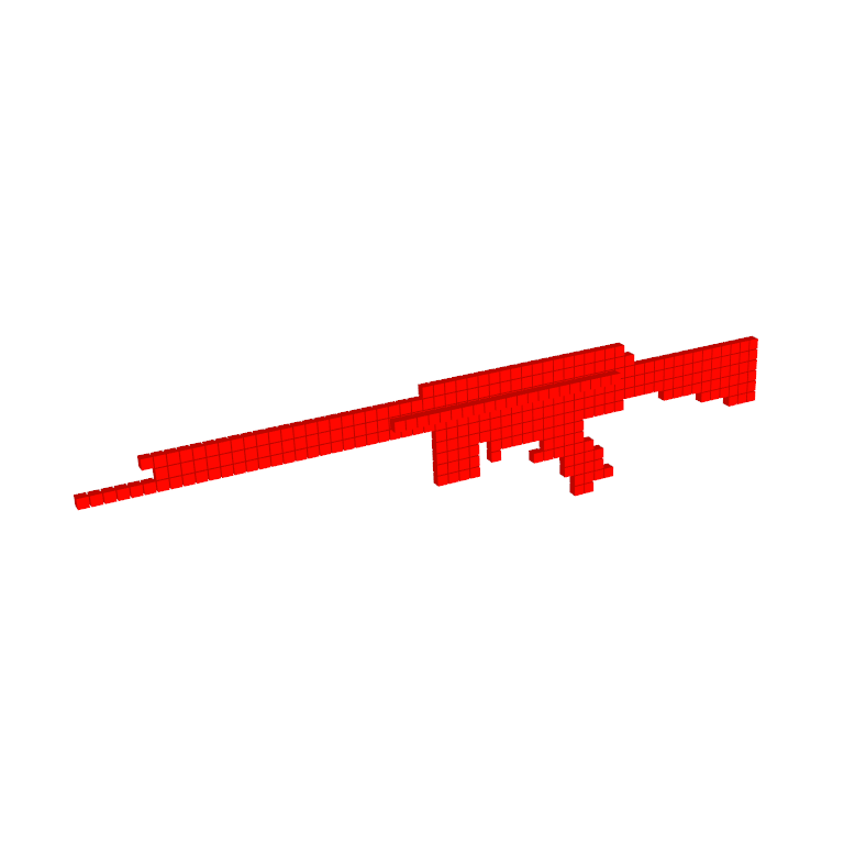
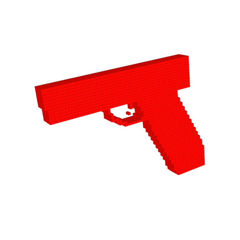
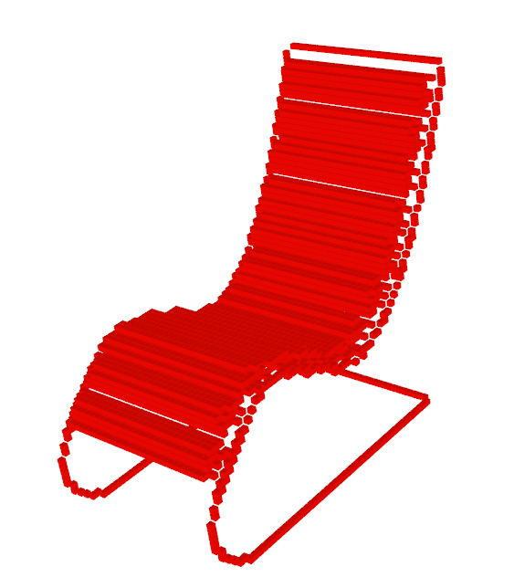
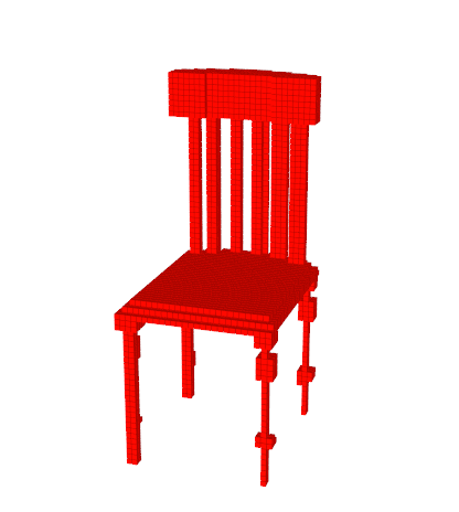
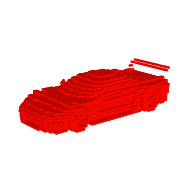
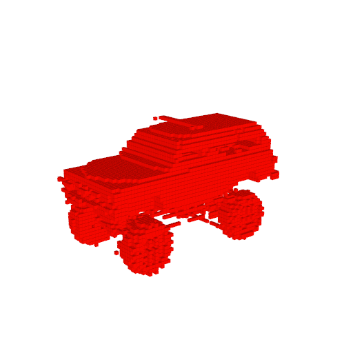
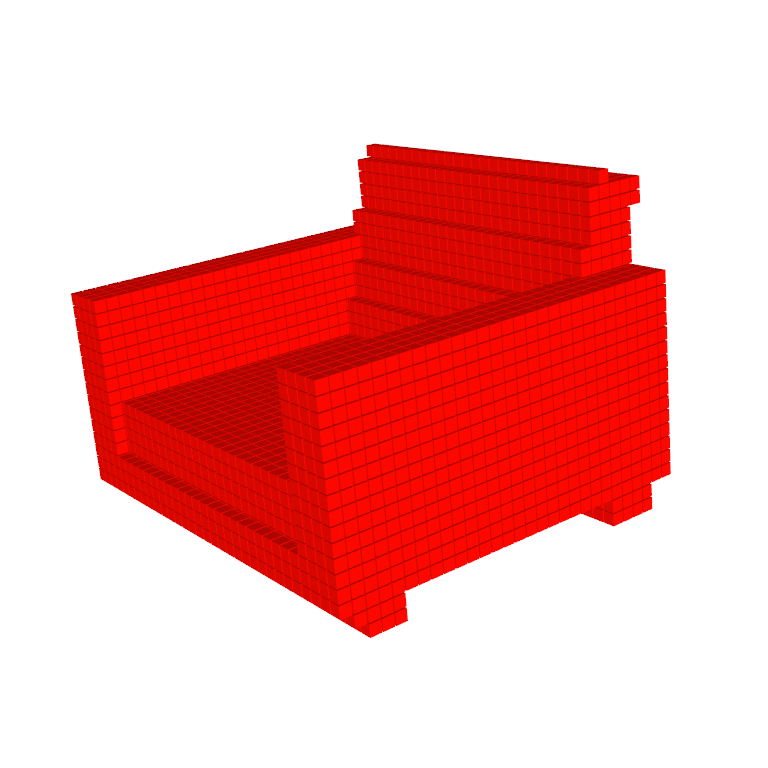
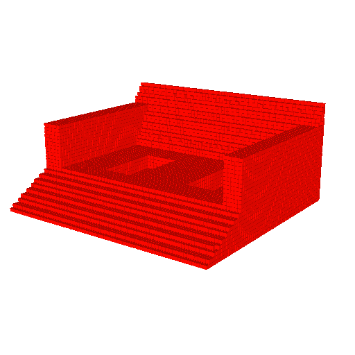
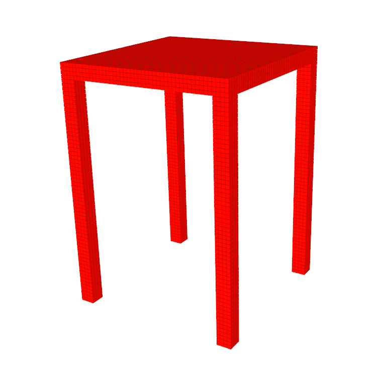
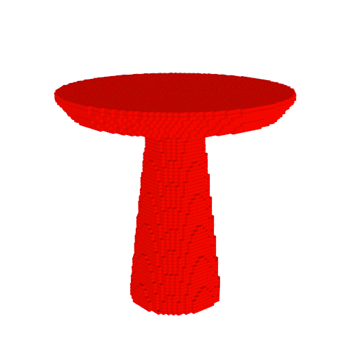
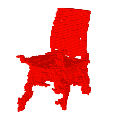
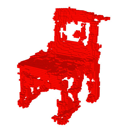
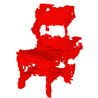
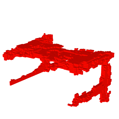
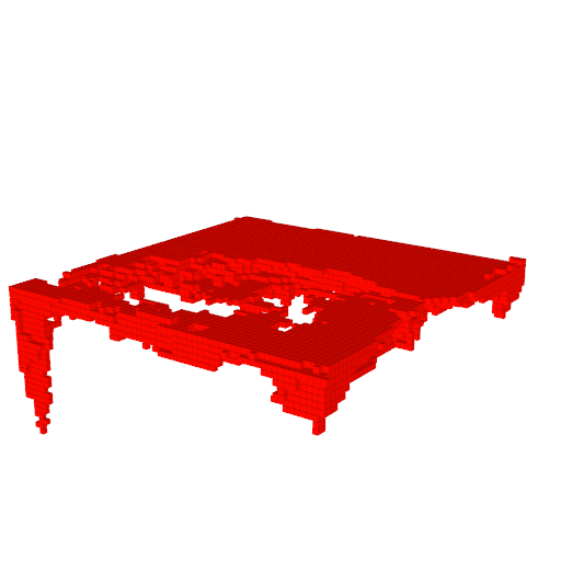
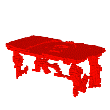
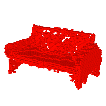
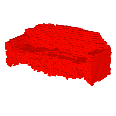
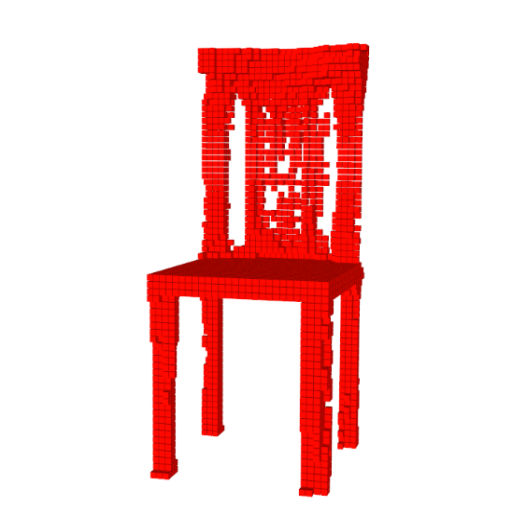
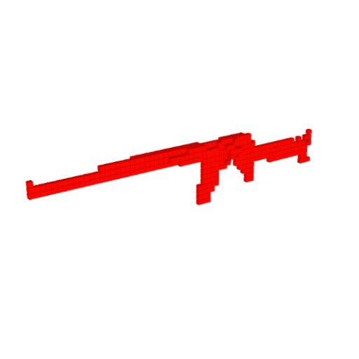
Figure 2 shows 3D objects generated by our 3D-GAN. For this experiment, we train one 3D-GAN for each object category. For generation, we sample -dimensional vectors following an i.i.d. uniform distribution over , and render the largest connected component of each generated object. We compare 3D-GAN with Wu et al. (2015), the state-of-the-art in 3D object synthesis from a probabilistic space, and with a volumetric autoencoder, whose variants have been employed by multiple recent methods (Girdhar et al., 2016; Sharma et al., 2016). Because an autoencoder does not restrict the distribution of its latent representation, we compute the empirical distribution of the latent vector of all training examples, fit a Gaussian distribution to , and sample from . Our algorithm produces 3D objects with much higher quality and more fine-grained details.
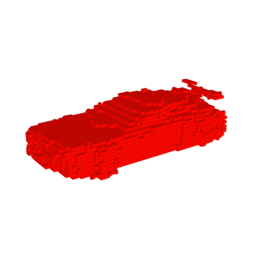
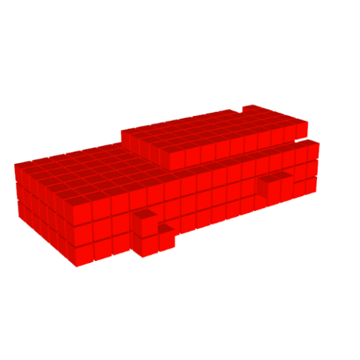
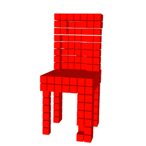
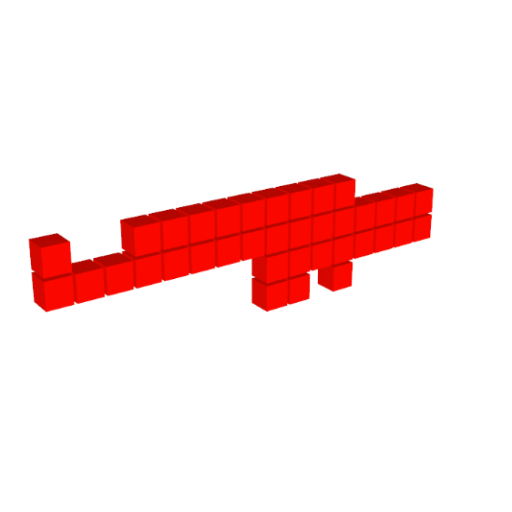
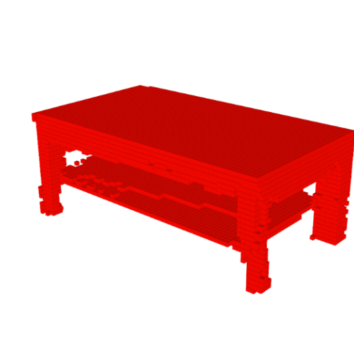
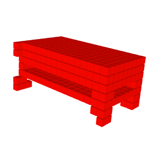
Compared with previous works, our 3D-GAN can synthesize high-resolution 3D objects with detailed geometries. Figure 3 shows both high-res voxels and down-sampled low-res voxels for comparison. Note that it is relatively easy to synthesize a low-res object, but is much harder to obtain a high-res one due to the rapid growth of 3D space. However, object details are only revealed in high resolution.
A natural concern to our generative model is whether it is simply memorizing objects from training data. To demonstrate that the network can generalize beyond the training set, we compare synthesized objects with their nearest neighbor in the training set. Since the retrieval objects based on distance in the voxel space are visually very different from the queries, we use the output of the last convolutional layer in our discriminator (with a 2x pooling) as features for retrieval instead. Figure 2 shows that generated objects are similar, but not identical, to the nearest examples in the training set.
| Supervision | Pretraining | Method | Classification (Accuracy) | |
| ModelNet40 | ModelNet10 | |||
| Category labels | ImageNet | MVCNN (Su et al., 2015a) | 90.1% | - |
| MVCNN-MultiRes (Qi et al., 2016) | 91.4% | - | ||
| None | 3D ShapeNets (Wu et al., 2015) | 77.3% | 83.5% | |
| DeepPano (Shi et al., 2015) | 77.6% | 85.5% | ||
| VoxNet (Maturana and Scherer, 2015) | 83.0% | 92.0% | ||
| ORION (Sedaghat et al., 2016) | - | 93.8% | ||
| Unsupervised | - | SPH (Kazhdan et al., 2003) | 68.2% | 79.8% |
| LFD (Chen et al., 2003) | 75.5% | 79.9% | ||
| T-L Network (Girdhar et al., 2016) | 74.4% | - | ||
| VConv-DAE (Sharma et al., 2016) | 75.5% | 80.5% | ||
| 3D-GAN (ours) | 83.3% | 91.0% | ||


| Method | Bed | Bookcase | Chair | Desk | Sofa | Table | Mean |
| AlexNet-fc8 (Girdhar et al., 2016) | 29.5 | 17.3 | 20.4 | 19.7 | 38.8 | 16.0 | 23.6 |
| AlexNet-conv4 (Girdhar et al., 2016) | 38.2 | 26.6 | 31.4 | 26.6 | 69.3 | 19.1 | 35.2 |
| T-L Network (Girdhar et al., 2016) | 56.3 | 30.2 | 32.9 | 25.8 | 71.7 | 23.3 | 40.0 |
| 3D-VAE-GAN (jointly trained) | 49.1 | 31.9 | 42.6 | 34.8 | 79.8 | 33.1 | 45.2 |
| 3D-VAE-GAN (separately trained) | 63.2 | 46.3 | 47.2 | 40.7 | 78.8 | 42.3 | 53.1 |



|





|
 |
 |
|
|
|
|
|
|
4.2 3D Object Classification
We then evaluate the representations learned by our discriminator. A typical way of evaluating representations learned without supervision is to use them as features for classification. To obtain features for an input 3D object, we concatenate the responses of the second, third, and fourth convolution layers in the discriminator, and apply max pooling of kernel sizes , respectively. We use a linear SVM for classification.
Data
We train a single 3D-GAN on the seven major object categories (chairs, sofas, tables, boats, airplanes, rifles, and cars) of ShapeNet (Chang et al., 2015). We use ModelNet (Wu et al., 2015) for testing, following Sharma et al. (2016); Maturana and Scherer (2015); Qi et al. (2016).***For ModelNet, there are two train/test splits typically used. Qi et al. (2016); Shi et al. (2015); Maturana and Scherer (2015) used the train/test split included in the dataset, which we also follow; Wu et al. (2015); Su et al. (2015a); Sharma et al. (2016) used training points and test points in each category for experiments, possibly with viewpoint augmentation. Specifically, we evaluate our model on both ModelNet10 and ModelNet40, two subsets of ModelNet that are often used as benchmarks for 3D object classification. Note that the training and test categories are not identical, which also shows the out-of-category generalization power of our 3D-GAN.
Results
We compare with the state-of-the-art methods (Wu et al., 2015; Girdhar et al., 2016; Sharma et al., 2016; Sedaghat et al., 2016) and show per-class accuracy in Table 1. Our representation outperforms other features learned without supervision by a large margin ( vs. on ModelNet40, and vs on ModelNet10) (Girdhar et al., 2016; Sharma et al., 2016). Further, our classification accuracy is also higher than some recent supervised methods (Shi et al., 2015), and is close to the state-of-the-art voxel-based supervised learning approaches (Maturana and Scherer, 2015; Sedaghat et al., 2016). Multi-view CNNs (Su et al., 2015a; Qi et al., 2016) outperform us, though their methods are designed for classification, and require rendered multi-view images and an ImageNet-pretrained model.
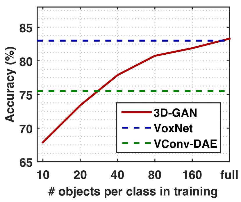
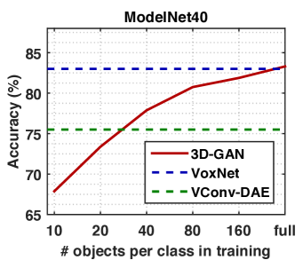
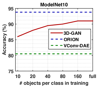
3D-GAN also works well with limited training data. As shown in Figure 6, with roughly 25 training samples per class, 3D-GAN achieves comparable performance on ModelNet40 with other unsupervised learning methods trained with at least 80 samples per class.
4.3 Single Image 3D Reconstruction
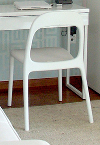
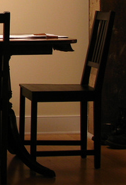
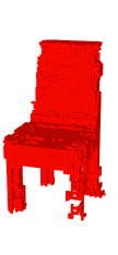
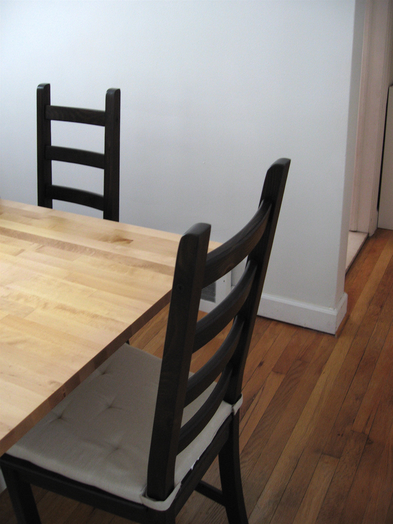
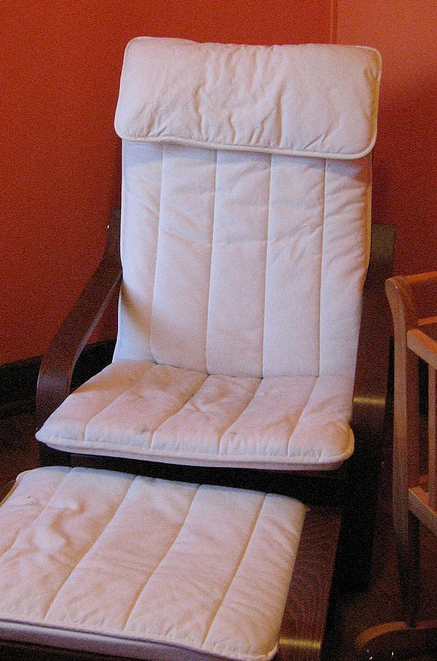
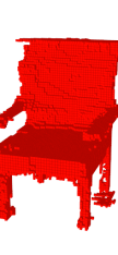
As an application, our show that the 3D-VAE-GAN can perform well on single image 3D reconstruction. Following previous work (Girdhar et al., 2016), we test it on the IKEA dataset (Lim et al., 2013), and show both qualitative and quantitative results.
Data
The IKEA dataset consists of images with IKEA objects. We crop the images so that the objects are centered in the images. Our test set consists of objects cropped from images (supplied by the author). The IKEA dataset is challenging because all images are captured in the wild, often with heavy occlusions. We test on all six categories of objects: bed, bookcase, chair, desk, sofa, and table.
Results
We show our results in Figure 7 and Table 2, with performance of a single 3D-VAE-GAN jointly trained on all six categories, as well as the results of six 3D-VAE-GANs separately trained on each class. Following Girdhar et al. (2016), we evaluate results at resolution , use the average precision as our evaluation metric, and attempt to align each prediction with the ground-truth over permutations, flips, and translational alignments (up to 10%), as IKEA ground truth objects are not in a canonical viewpoint. In all categories, our model consistently outperforms previous state-of-the-art in voxel-level prediction and other baseline methods.†††For methods from Girdhar et al. (2016), the mean values in the last column are higher than the originals in their paper, because we compute per-class accuracy instead of per-instance accuracy.
5 Analyzing Learned Representations
In this section, we look deep into the representations learned by both the generator and the discriminator of 3D-GAN. We start with the -dimensional object vector, from which the generator produces various objects. We then visualize neurons in the discriminator, and demonstrate that these units capture informative semantic knowledge of the objects, which justifies its good performance on object classification presented in Section 4.
5.1 The Generative Representation
We explore three methods for understanding the latent space of vectors for object generation. We first visualize what an individual dimension of the vector represents; we then explore the possibility of interpolating between two object vectors and observe how the generated objects change; last, we present how we can apply shape arithmetic in the latent space.
Visualizing the object vector
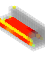
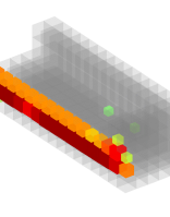
To visualize the semantic meaning of each dimension, we gradually increase its value, and observe how it affects the generated 3D object. In Figure 6, each column corresponds to one dimension of the object vector, where the red region marks the voxels affected by changing values of that dimension. We observe that some dimensions in the object vector carries semantic knowledge of the object, e.g., the thickness or width of surfaces.
Interpolation
We show results of interpolating between two object vectors in Figure 6. Earlier works demonstrated interpolation between two 2D images of the same category (Dosovitskiy et al., 2015; Radford et al., 2016). Here we show interpolations both within and across object categories. We observe that for both cases walking over the latent space gives smooth transitions between objects.
Arithmetic
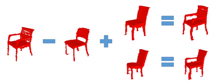
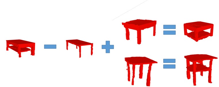
Another way of exploring the learned representations is to show arithmetic in the latent space. Previously, Dosovitskiy et al. (2015); Radford et al. (2016) presented that their generative nets are able to encode semantic knowledge of chair or face images in its latent space; Girdhar et al. (2016) also showed that the learned representation for 3D objects behave similarly. We show our shape arithmetic in Figure 8. Different from Girdhar et al. (2016), all of our objects are randomly sampled, requiring no existing 3D CAD models as input.
5.2 The Discriminative Representation
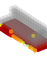
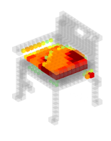
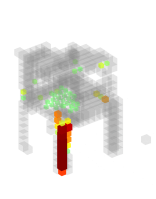
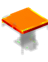
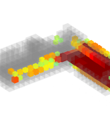
We now visualize the neurons in the discriminator. Specifically, we would like to show what input objects, and which part of them produce the highest intensity values for each neuron. To do that, for each neuron in the second to last convolutional layer of the discriminator, we iterate through all training objects and exhibit the ones activating the unit most strongly. We further use guided back-propagation (Springenberg et al., 2015) to visualize the parts that produce the activation.
Figure 9 shows the results. There are two main observations: first, for a single neuron, the objects producing strongest activations have very similar shapes, showing the neuron is selective in terms of the overall object shape; second, the parts that activate the neuron, shown in red, are consistent across these objects, indicating the neuron is also learning semantic knowledge about object parts.
6 Conclusion
In this paper, we proposed 3D-GAN for 3D object generation, as well as 3D-VAE-GAN for learning an image to 3D model mapping. We demonstrated that our models are able to generate novel objects and to reconstruct 3D objects from images. We showed that the discriminator in GAN, learned without supervision, can be used as an informative feature representation for 3D objects, achieving impressive performance on shape classification. We also explored the latent space of object vectors, and presented results on object interpolation, shape arithmetic, and neuron visualization.
Acknowledgement
This work is supported by NSF grants #1212849 and #1447476, ONR MURI N00014-16-1-2007, the Center for Brain, Minds and Machines (NSF STC award CCF-1231216), Toyota Research Institute, Adobe, Shell, IARPA MICrONS, and a hardware donation from Nvidia.
References
- Bansal et al. [2016] Aayush Bansal, Bryan Russell, and Abhinav Gupta. Marr revisited: 2d-3d alignment via surface normal prediction. In CVPR, 2016.
- Blanz and Vetter [1999] Volker Blanz and Thomas Vetter. A morphable model for the synthesis of 3d faces. In SIGGRAPH, 1999.
- Carlson [1982] Wayne E Carlson. An algorithm and data structure for 3d object synthesis using surface patch intersections. In SIGGRAPH, 1982.
- Chang et al. [2015] Angel X Chang, Thomas Funkhouser, Leonidas Guibas, et al. Shapenet: An information-rich 3d model repository. arXiv preprint arXiv:1512.03012, 2015.
- Chaudhuri et al. [2011] Siddhartha Chaudhuri, Evangelos Kalogerakis, Leonidas Guibas, and Vladlen Koltun. Probabilistic reasoning for assembly-based 3d modeling. ACM TOG, 30(4):35, 2011.
- Chen et al. [2003] Ding-Yun Chen, Xiao-Pei Tian, Yu-Te Shen, and Ming Ouhyoung. On visual similarity based 3d model retrieval. CGF, 2003.
- Choy et al. [2016] Christopher B Choy, Danfei Xu, JunYoung Gwak, Kevin Chen, and Silvio Savarese. 3d-r2n2: A unified approach for single and multi-view 3d object reconstruction. In ECCV, 2016.
- Denton et al. [2015] Emily L Denton, Soumith Chintala, and Rob Fergus. Deep generative image models using a laplacian pyramid of adversarial networks. In NIPS, 2015.
- Dosovitskiy et al. [2015] Alexey Dosovitskiy, Jost Tobias Springenberg, and Thomas Brox. Learning to generate chairs with convolutional neural networks. In CVPR, 2015.
- Girdhar et al. [2016] Rohit Girdhar, David F Fouhey, Mikel Rodriguez, and Abhinav Gupta. Learning a predictable and generative vector representation for objects. In ECCV, 2016.
- Goodfellow et al. [2014] Ian Goodfellow, Jean Pouget-Abadie, Mehdi Mirza, Bing Xu, David Warde-Farley, Sherjil Ozair, Aaron Courville, and Yoshua Bengio. Generative adversarial nets. In NIPS, 2014.
- Huang et al. [2015] Haibin Huang, Evangelos Kalogerakis, and Benjamin Marlin. Analysis and synthesis of 3d shape families via deep-learned generative models of surfaces. CGF, 34(5):25–38, 2015.
- Im et al. [2016] Daniel Jiwoong Im, Chris Dongjoo Kim, Hui Jiang, and Roland Memisevic. Generating images with recurrent adversarial networks. arXiv preprint arXiv:1602.05110, 2016.
- Kalogerakis et al. [2012] Evangelos Kalogerakis, Siddhartha Chaudhuri, Daphne Koller, and Vladlen Koltun. A probabilistic model for component-based shape synthesis. ACM TOG, 31(4):55, 2012.
- Kar et al. [2015] Abhishek Kar, Shubham Tulsiani, Joao Carreira, and Jitendra Malik. Category-specific object reconstruction from a single image. In CVPR, 2015.
- Kazhdan et al. [2003] Michael Kazhdan, Thomas Funkhouser, and Szymon Rusinkiewicz. Rotation invariant spherical harmonic representation of 3 d shape descriptors. In SGP, 2003.
- Kingma and Ba [2015] Diederik P Kingma and Jimmy Ba. Adam: A method for stochastic optimization. In ICLR, 2015.
- Kingma and Welling [2014] Diederik P Kingma and Max Welling. Auto-encoding variational bayes. In ICLR, 2014.
- Larsen et al. [2016] Anders Boesen Lindbo Larsen, Søren Kaae Sønderby, and Ole Winther. Autoencoding beyond pixels using a learned similarity metric. In ICML, 2016.
- Li and Wand [2016] Chuan Li and Michael Wand. Precomputed real-time texture synthesis with markovian generative adversarial networks. arXiv preprint arXiv:1604.04382, 2016.
- Li et al. [2015] Yangyan Li, Hao Su, Charles Ruizhongtai Qi, Noa Fish, Daniel Cohen-Or, and Leonidas J Guibas. Joint embeddings of shapes and images via cnn image purification. ACM TOG, 34(6):234, 2015.
- Lim et al. [2013] Joseph J. Lim, Hamed Pirsiavash, and Antonio Torralba. Parsing ikea objects: Fine pose estimation. In ICCV, 2013.
- Maas et al. [2013] Andrew L Maas, Awni Y Hannun, and Andrew Y Ng. Rectifier nonlinearities improve neural network acoustic models. In ICML, 2013.
- Maturana and Scherer [2015] Daniel Maturana and Sebastian Scherer. Voxnet: A 3d convolutional neural network for real-time object recognition. In IROS, 2015.
- Qi et al. [2016] Charles R Qi, Hao Su, Matthias Niessner, Angela Dai, Mengyuan Yan, and Leonidas J Guibas. Volumetric and multi-view cnns for object classification on 3d data. In CVPR, 2016.
- Radford et al. [2016] Alec Radford, Luke Metz, and Soumith Chintala. Unsupervised representation learning with deep convolutional generative adversarial networks. In ICLR, 2016.
- Rezende et al. [2016] Danilo Jimenez Rezende, SM Eslami, Shakir Mohamed, Peter Battaglia, Max Jaderberg, and Nicolas Heess. Unsupervised learning of 3d structure from images. In NIPS, 2016.
- Sedaghat et al. [2016] Nima Sedaghat, Mohammadreza Zolfaghari, and Thomas Brox. Orientation-boosted voxel nets for 3d object recognition. arXiv preprint arXiv:1604.03351, 2016.
- Sharma et al. [2016] Abhishek Sharma, Oliver Grau, and Mario Fritz. Vconv-dae: Deep volumetric shape learning without object labels. arXiv preprint arXiv:1604.03755, 2016.
- Shi et al. [2015] Baoguang Shi, Song Bai, Zhichao Zhou, and Xiang Bai. Deeppano: Deep panoramic representation for 3-d shape recognition. IEEE SPL, 22(12):2339–2343, 2015.
- Springenberg et al. [2015] Jost Tobias Springenberg, Alexey Dosovitskiy, Thomas Brox, and Martin Riedmiller. Striving for simplicity: The all convolutional net. In ICLR Workshop, 2015.
- Su et al. [2015a] Hang Su, Subhransu Maji, Evangelos Kalogerakis, and Erik Learned-Miller. Multi-view convolutional neural networks for 3d shape recognition. In ICCV, 2015a.
- Su et al. [2015b] Hao Su, Charles R Qi, Yangyan Li, and Leonidas Guibas. Render for cnn: Viewpoint estimation in images using cnns trained with rendered 3d model views. In ICCV, 2015b.
- Tangelder and Veltkamp [2008] Johan WH Tangelder and Remco C Veltkamp. A survey of content based 3d shape retrieval methods. Multimedia tools and applications, 39(3):441–471, 2008.
- Van Kaick et al. [2011] Oliver Van Kaick, Hao Zhang, Ghassan Hamarneh, and Daniel Cohen-Or. A survey on shape correspondence. CGF, 2011.
- Wang and Gupta [2016] Xiaolong Wang and Abhinav Gupta. Generative image modeling using style and structure adversarial networks. In ECCV, 2016.
- Wu et al. [2016] Jiajun Wu, Tianfan Xue, Joseph J Lim, Yuandong Tian, Joshua B Tenenbaum, Antonio Torralba, and William T Freeman. Single image 3d interpreter network. In ECCV, 2016.
- Wu et al. [2015] Zhirong Wu, Shuran Song, Aditya Khosla, Fisher Yu, Linguang Zhang, Xiaoou Tang, and Jianxiong Xiao. 3d shapenets: A deep representation for volumetric shapes. In CVPR, 2015.
- Xiang et al. [2015] Yu Xiang, Wongun Choi, Yuanqing Lin, and Silvio Savarese. Data-driven 3d voxel patterns for object category recognition. In CVPR, 2015.
- Xiao et al. [2010] Jianxiong Xiao, James Hays, Krista Ehinger, Aude Oliva, and Antonio Torralba. Sun database: Large-scale scene recognition from abbey to zoo. In CVPR, 2010.
- Xue et al. [2012] Tianfan Xue, Jianzhuang Liu, and Xiaoou Tang. Example-based 3d object reconstruction from line drawings. In CVPR, 2012.
- Yan et al. [2016] Xinchen Yan, Jimei Yang, Ersin Yumer, Yijie Guo, and Honglak Lee. Perspective transformer nets: Learning single-view 3d object reconstruction without 3d supervision. In NIPS, 2016.
- Zhu et al. [2016] Jun-Yan Zhu, Philipp Krähenbühl, Eli Shechtman, and Alexei A Efros. Generative visual manipulation on the natural image manifold. In ECCV, 2016.
Appendix A.1 Network Structure
Here we give the network structures of the generator, the discriminator, and the image encoder.
Generator The generator consists of five fully convolution layers with numbers of channels , kernel sizes , and strides . We add ReLU and batch normalization layers between convolutional layers, and a Sigmoid layer at the end. The input is a -dimensional vector, and the output is a matrix with values in .
Discriminator As a mirrored version of the generator, the discriminator takes as input a matrix, and outputs a real number in . The discriminator consists of volumetric convolution layers, with numbers of channels , kernel sizes , and strides . There are leaky ReLU layers of parameter and batch normalization layers in between, and a Sigmoid layer at the end.
Image encoder The image encoder in our 3D-VAE-GAN takes a image as input, and outputs a -dimensional vector. It consists of five spatial convolution layers with numbers of channels , kernel sizes , and strides , respectively. There are ReLU and batch normalization layers in between. The output of the last convolution layer is a -dimensional vector representing a Gaussian distribution in the -dimensional space, where dimensions are for the mean and the other dimensions are for the diagonal variance. There is a sampling layer at the end to sample a -dimensional vector from the Gaussian distribution, which is later used by the 3D-GAN.
Appendix A.2 3D Shape Classification
Here we present the details of our shape classification experiments. For each object, we take the responses of the second, third, and fourth convolution layers of the discriminator, and apply max pooling of kernel sizes , respectively. We then concatenate the outputs into a vector of length , which is later used by a linear SVM for training and classification.
We use one-versus-all SVM classifiers. We use L2 penalty, balanced class weights, and intercept scaling during training. For ModelNet40, we train a linear SVM with penalty parameter , and for ModelNet10, we have . We also show the results with limited training data on both ModelNet40 and ModelNet10 in Figure A1.
Appendix A.3 3D-VAE-GAN Training
Let be the set of training pairs, where is a 2D image and is the corresponding 3D shape. In each iteration of training, we first generate a random sample from ‡‡‡ is an identity matrix.. Then we update the discriminator , the image encoder , and the generator sequentially. Specifically,
-
•
Step 1: Update the discriminator by minimizing the following loss function:
(6) -
•
Step 2: Update the image encoder by minimizing the following loss function:
(7) where and are the predicted mean and variance of the latent variable , respectively.
-
•
Step 3: Update the generator by minimizing the following loss function:
(8)