Magnetic flux density from the relative circular motion of stars and partially ionized gas in the Galaxy mid-plane vicinity

Joanna Jałocha¹, Łukasz Bratek^2,⋆, Jan Pȩkala², Szymon Sikora³, Marek Kutschera⁴
1. Institute of Physics, Cracow University of Technology, PL-30084 Krakow, Poland 2. Institute of Nuclear Physics, Polish Academy of Sciences, PL-31342 Krakow, Poland 3. Astronomical Observatory, Jagellonian University, PL-30244 Krakow, Poland 4. Institute of Physics, Jagellonian University, PL-30059 Krakow, Poland

Preprint v1, 24 OCT 2016, IFJPAN-IV-2016-25

Abstract. Observations suggest a slower stellar rotation relative to gas rotation in the outer part of the Milky Way Galaxy. This difference could be attributed to an interaction with the interstellar magnetic field. In a simple model, fields of order $10\,\mu\mathrm{G}$ are then required, consistently with the observed values. This coincidence suggests a tool for estimating magnetic fields in spiral galaxies. A North-South asymmetry in the rotation of gas in the Galaxy could be of magnetic origin too.

1 Introduction

The mechanism of the influence of turbulent and large-scale magnetic fields on the motion of the gaseous fraction was described in the context of galactic dynamics by Battaner et al., [1992]. The interstellar gas is ionized to a degree sufficient for the magnetic field to freeze-in the gas, so that the resulting magnetic tension can be assumed to hold the gas and so influence its motion, modifying the predictions of purely gravitational models. Because the gas density decreases with the galactocentric distance, the magnetic effect becomes important for larger radii.

There have been several works devoted to this problem so far, showing that magnetic fields of a few$\,\mu\mathrm{G}$ (typical for the interstellar medium in spiral galaxies) are capable of considerably influencing the kinematics of (at least) partially ionized gas [Battaner et al.,, 1992, 2008; Kutschera and Jałocha,, 2004; Battaner and Florido,, 2007; Ruiz-Granados et al., 2010b, ; Ruiz-Granados et al.,, 2012; Jałocha et al., 2012a, ; Jałocha et al., 2012b, ]. The fields have the potential to modify the outer parts of gaseous rotation curves, and in turn, the predictions about the distribution of mass.

Magnetic fields can not be ignored when one attempts to fully understand the problem of rotation of spiral galaxies. Battaner et al., [1992] brought to attention the possibility that the observed flatness of outer disc rotation curves, or even their rise, could be simply the result of interaction with interstellar magnetic fields (not merely due to unseen dark matter halo). In particular, it might turn out, that taking magnetic fields into account would reduce the amount of non-baryonic dark matter required by models that ignore magnetic fields.

Interestingly, using position-velocity data for a sample of remote classical cepheids and for HII regions in the Galaxy, Pont et al., [1997] found that the rotation curve indicated by the stars in the outer disc is markedly lower than the rotation curve of gas in the same region. They attributed this difference to either non-axisymmetric components in the gas motion, or to high uncertainties in the distances to HII regions. From [Pont et al.,, 1997] it is evident also that there is a South-North asymmetry of the gaseous rotation curve, not observed for the stellar rotation curve. Remarkably, the difference in the rotation curves concerns the outer part of the Galactic disc and increases with the Galactocentric distance. The difference seems too high to be solely due to the neglected velocity components. Rather, the differences may be a manifestation of the influence of magnetic fields acting upon the gaseous substructure, increasing the rotation of gas with respect to that of stars. By neglecting magnetic fields, this increase would be customarily attributed to higher amounts of dark matter distributed in outer regions.

So far, the studies on the influence of magnetic fields on rotation curves have been inconclusive. Some authors, e.g. Battaner and Florido, [2007]; Ruiz-Granados et al., [2012], state that magnetic fields are responsible for the flattening or rise of outer parts of rotation curves, other authors provide sound arguments that the influence is unlikely, or even may impede the gravitationally supported rotation, leading to an even higher halo mass [Sánchez-Salcedo and Santillán,, 2013; Elstner et al.,, 2014]. However, the effects are subject to modelling assumptions.

The motivation behind the present work is our conjecture, that the observed difference between the stellar and gaseous rotation curves of the Milky Way galaxy can be explained by the influence of magnetic fields. With this assumption, we estimate the magnitude and profiles of the radial and azimuthal magnetic field components required to account for the difference in rotation.

2 Gaseous and stellar rotation curves

The Milky Way rotation curve is determined based on the measurements of various kinematical tracers moving in the Galactic plane vicinity. To obtain the stellar and gaseous rotation curves, we unified position-velocity data for $357$ cepheids [Caldwell and Coulson,, 1987; Pont et al.,, 1994, 1997; Berdnikov et al.,, 2000; Mel’nik et al.,, 2015], $110$ carbon stars [Demers and Battinelli,, 2007; Battinelli et al.,, 2013] and $255$ HII regions [Blitz et al.,, 1982; Chini and Wink,, 1984; Fich et al.,, 1989; Brand and Blitz,, 1993]. The data were originally used as tracers of rotation in the Galactic plane vicinity, therefore we do not perform any further selection. We transformed the radial distances, radial motions and transverse motions (and the respective errors) from the heliocentric coordinate frame to the Galactocentric coordinate frame, assuming the IAU Galactic constants $R_{o}=8.5\,\mathrm{kpc}$ and $V_{o}=220\,\mathrm{km}/\!\sec$. For each data point we found the projected distance and the azimuthal velocity component in the Galactic plane (that is, $R$ and $R\cdot\mathrm{d}\Phi/\mathrm{d}t$ in cylindrical coordinates). We denote them as $(r_{i},v_{i})$ pairs.

To obtain a rotation curve from a set $\mathcal{S}=\{(r_{i},v_{i})\}_{1\leq i\leq n}$, we start with a distribution function $\tilde{p}(r,v)=\tilde{\mathcal{N}}_{S}^{-1}\sum_{i=1}^{n}\exp\left(-\frac{(r-r_{i})^{2}}{2\left(\Delta r_{i}\right)^{2}}-\frac{(v-v_{i})^{2}}{2\left(\Delta v_{i}\right)^{2}}\right)$, $\tilde{\mathcal{N}}_{\mathcal{S}}$ being an $\mathcal{S}$-dependent normalization constant, and $\Delta r_{i}$ and $\Delta v_{i}$ the measurement uncertainties. To simplify calculations without noticeably changing the results, the integration regions were formally extended to $\pm\infty$ in both $R$ and $V$ variables, because the summands in $\tilde{p}$ are rapidly decreasing outside a convex region encompassing entire $\mathcal{S}$. Next, we form a related smoothed-out distribution function $p$ by integrating $\tilde{p}$ within intervals $(R-w/2,R+w/2)$: $p(R,V)=\mathcal{N}_{S}^{-1}\sum_{i=1}^{n}\exp\left(-\frac{(V-v_{i})^{2}}{2\left(\Delta v_{i}\right)^{2}}\right)f_{w,i}(R)$ where $f_{w,i}(R)=\frac{1}{2w}\left(\mathrm{erf}\left(\frac{R-r_{i}+w/2}{\sqrt{2}\Delta r_{i}}\right)-\mathrm{erf}\left(\frac{R-r_{i}-w/2}{\sqrt{2}\Delta r_{i}}\right)\right)$ are integrable to $1$ on the interval $R\in\left(-\infty,+\infty\right)$. Then, corresponding to $p(R,V)$, the conditional expectation value of $V$ denoted by $E_{V}(R)$ and its dispersion measure $S_{V}(R)$ read (the summation is taken over all tracers):

$$E_{V}(R) = \frac{\sum_{i=1}^{n}v_{i}f_{w,i}(R)}{\sum_{i=1}^{n}f_{w,i}(R)},$$

$$S_{V}(R) = \sqrt{\frac{\sum_{i=1}^{n}\left(\left(E_{V}(R)-v_{i}\right)^{2}+\left(\Delta v_{i}\right)^{2}\right)f_{w,i}(R)}{\sum_{i=1}^{n}f_{w,i}(R)}}{.}$$

Note, that the $S_{V}(R)$ involves both the uncertainties $\Delta v_{i}$ and $\Delta r_{i}$. We chose the window width $w\approx 1.5\,\mathrm{kpc}$ for so defined moving averages $E_{V}$ and $S_{V}$. The moving average lines were then smoothed-out using a smoothing spline interpolation method. So obtained gaseous and stellar rotation curves are plotted in Fig.1, together with their respective conditional density distributions.

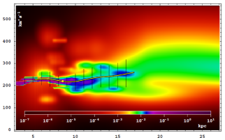
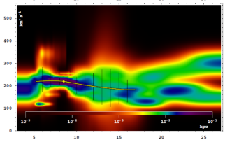
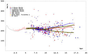
Figure 1: Conditional distribution function for position-velocity measurements in Galactic coordinates (assuming IAU Galactic constants $R_{o}=8.5\,\mathrm{kpc}$ and $V_{o}=220\,\mathrm{km}/\!\sec$, indicated on the graphs with the yellow dot), for gas [top panel] and for stars (unified data for cepheids and carbon stars) [middle panel] respectively, which we used to obtain gaseous and stellar rotation curves shown here with black-yellow lines (the vertical thin lines represent a region within a deviation $S_{V}(R)$ from the mean $E_{V}(R)$). The position-velocity points are shown explicitly [bottom panel], together with the stellar and gaseous rotation curves from upper panels. The red solid line and the blue solid line show the rotation curves for the gas above and below the Galactic plane, respectively. To verify our method of obtaining the rotation curves, we show with the black thin line an independent gaseous rotation curve of Galaxy, reproduced from a polynomial fit to gas position-velocity data published by Clemens, [1985] (assuming the same IAU Galactic constants).

For the purpose of this paper, the stellar and gaseous rotation curves were made to coincide at the point $(R_{o},V_{o})$, even though fractions of galactic material in the neighborhood of the Local Standard of Rest perform a small relative motion. But, if we are to compute the magnetic field necessary to obtain a given difference between two rotation curves, first we have to exclude any contribution to the actual difference, which is known to be of non-magnetic origin. The latter will certainly be dominating, because the density of gas in the vicinity of the circular orbit $R=R_{o}$ is too high for the magnetic field to be dynamically important, compared with the gravitational interaction.

Now, we come back to the observational fact reported by Pont et al., [1997], that the stellar rotation curve is markedly lower in the outer disc region than the rotation curve of gas. This is also true for the rotation curves in Fig.1, which shows that the separation effect is not changed by considering an extended sample of stars and by applying an independent averaging method. The South-North asymmetry in the rotation of gas has appeared too. In addition, a South-North asymmetry in the motion of stars is visible, but it is lower than that for gas and has variable sign – higher velocities closer to $R_{o}$ are observed for stars on the Southern side, then, for greater $R$, on the Northern side.

The dispersion measure $S_{V}(R)$ of observed azimuthal velocities of kinematical tracers about the mean value $E_{V}(R)$, defined earlier and shown in Fig.1 separately for stars and for gas, is comparable with the separation of the stellar and gaseous rotation curves. It is true that the separation may be entirely due to measurement inaccuracies, and Pont et al., [1997] discuss a possible explanation, but the separation is also markedly large. The dilemma can be solved only by increasing the accuracy of measurements. Our hypothesis is that the whole effect (or its significant part) may be caused by the presence of large scale magnetic fields. Then, important is the real amount of the separation, although it might slightly differ from that seen in Fig.1.

Before proceeding further, it should be tested, if the lack of complete information about the transversal motions for a number of heliocentric position-velocity data, may be consequential for the shape of the obtained stellar rotation curve, and sufficient to account for the observed difference in the rotation of stars and gas. A fraction of cepheids in the sample used to prepare the stellar rotation curve have all their three velocity components measured. We obtained for them two test rotation curves: one based on all three heliocentric velocity components, and the other based only on the radial heliocentric component (as if the transverse heliocentric components were unknown). The result is shown in Fig.2.

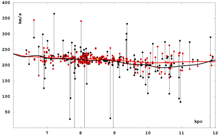
Figure 2: Rotation curves for cepheids with measured radial and transversal velocity components: [red]– true azimuthal component of Galactocentric velocity and a moving average fit obtained based on all three heliocentric components (the transformation parameters were constrained so that the circular velocity is $220\,\mathrm{km}/\sec$ at $8.5\,\mathrm{kpc}$); [black]– a re-projected azimuthal component and a moving average fit obtained based only on the heliocentric radial motion assuming the same transformation parameters as before.

There is a difference seen for the test curves, but it is very small in comparison to the separation between the stellar and gaseous rotation curves.

3 Gas density

Magnetic field can not directly influence the motion of neutral gas. The ionized gas fraction of the interstellar medium is more diluted than the non-ionized fraction. But, as explained in the introduction, it is dense enough for the magnetic field to be frozen-in and to hold together the mixture of gases (including molecular gas). The gas then moves as a whole driven by magnetic tension. Its column mass density $\sigma(R)$ can be thus reliably approximated by that of the neutral hydrogen. The latter we adopt from [Nakanishi and Sofue,, 2016] and, re-project to a volume density of the form:

$$\varrho(R,{Z})=\frac{\varrho_{o}(R)}{\cosh^{2}\left(\frac{1}{2}(Z/h)\right)},\qquad\varrho_{o}(R)=\frac{\sigma(R)}{4h}.$$ (1)

For $\left|Z\right|\gg h$, the profile function $\cosh^{-2}\left(\frac{1}{2}(Z/h)\right)$ behaves as $\exp\left(-|Z|/h\right)$, however $\varrho(R,Z)$ is smoother and half as high in the Galactic plane vicinity as the cuspy exponential profile $\frac{\sigma(R)}{2h}\exp\left(-|Z|/h\right)$ with the same integrated mass. The $\cosh^{-2}$ profile is a solution of the Jeans equation, under the assumption of negligible horizontal variations in the density, and almost uniform gravitational acceleration. The disc thickness is related to a width-scale parameter $h$, which is regarded as a single free parameter, assumed to be independent of $R$ (a region $-h<z<h$ comprises ${\sim}46\%$ of total mass).

The above volume density model with constant thickness is only a coarse grained approximation used to map a given column density $\sigma(R)$ to a central volume density $\varrho_{o}(R)$. Real disc thickness grows quickly in an exponential fashion with the Galactocentric distance [Kalberla et al.,, 2007], moreover, the gas disc warps [May et al.,, 1997] with asymmetric amplitude of a few $\,\mathrm{kpc}$ [Nakanishi and Sofue,, 2006; Levine et al.,, 2006]. Thus, it is not a priori obvious how the single model parameter $h$ relates to the real variable thickness of the warped disc. Moreover, our simplified magneto-hydrodynamical model (which we discuss in more detail later) neglects the vertical structure, thus the decrease in the density with $\left|Z\right|$ occurring when $h$ is very low must be accounted for. The HII regions which are used to determine the Galactic rotation curve and whose motion is influenced by magnetic fields, are located within a strip $|Z|<450\,\mathrm{pc}$ in which we assume that the fields and volume density are independent of $Z$. Now, for $h$ large enough, say $h=1.5\,\mathrm{kpc}$ or more, the volume density would change insignificantly within the strip and could be assumed constant (equal to the central volume density), however, for small $h$, say $h=450\mathrm{pc}$ or less, the decrease of the density could not be neglected (the easiest way would be to take in place of the central density some reduced, say, average density within the strip).

In Fig.3, the central volume density (at $Z=0$) corresponding to Eq.1, is shown for various $h$. In the same figure

Figure 3: Central volume density of the gaseous fraction (at $Z=0$) corresponding to the density profile in Eq.1, shown for various values of width-scale parameter $h$ [solid lines]. For comparison, the [dotted line] shows a volume density at $Z=0$ from [Kalberla and Kerp,, 2009].

is shown also a central volume density from [Kalberla and Kerp,, 2009]. As is seen, it is much higher than considered by us. We stress, that surface density in [Nakanishi and Sofue,, 2016] (based on which we obtain our volume densities) and surface density in [Kalberla and Kerp,, 2009] are very similar, therefore the difference in the volume densities results from differences in the assumptions made about the shape and thickness of the vertical profile of gas. Kalberla and Kerp, [2009] predict much lower half width at half maximum scale height than ours: in a region between $R_{o}$ and $2R_{o}$, it grows from $\approx 150\mathrm{pc}$ to $\approx 360\mathrm{pc}$, see Fig.6 in Kalberla and Kerp, [2009].

4 Magnetic fields

A magnetic field, necessary to account for the measured difference in the circular velocities, can be obtained by finding a solution of the stationary Navier-Stokes equation for an inviscid and pressureless medium:

$$\left(\vec{v}\circ\vec{\nabla}\right)\vec{v}=-\vec{\nabla}U+\frac{1}{4\pi\varrho}\left(\vec{\nabla}\times\vec{B}\right)\times\vec{B}.$$ (2)

The field $\vec{B}$ can be decomposed into a series of modes, lower modes for larger scale structures and higher modes for lower scale structures; each mode with its own amplitude, possibly some of them dominating all the others. The dominant part of the large-scale magnetic field of the Galaxy is likely to be axisymmetric, according to the turbulent dynamo theory and in agreement with observations [Vallee,, 1991]. Under axial symmetry and in the Galactic plane vicinity (where the vertical component $B_{Z}$ and its first derivative can be assumed to vanish by reflection symmetry with respect to that plane), the system of equations Eq.2 reduces to

$$V_{R}\,\frac{\partial V_{R}}{\partial R}=\frac{\delta\,v_{\Phi}^{2}}{R}-\frac{1}{4\pi\varrho}\,\frac{B_{\Phi}^{2}}{R}-\frac{1}{4\pi\varrho}\,B_{\Phi}\frac{\partial B_{\Phi}}{\partial R},$$ (3a)

$$V_{R}\frac{\partial\left({R}\,V_{\Phi|G}\right)}{\partial R}=\frac{1}{4\pi\varrho}\,B_{R}\frac{\partial\left({R}\,B_{\Phi}\right)}{\partial R}.$$ (3b)

Here, $\delta\,v_{\Phi}^{2}=V_{\Phi|G}^{2}-V_{\Phi|S}^{2}$ stands for a given difference of squares of circular velocities $V_{\Phi|G}$ and $V_{\Phi|S}$, that of gas and stars, respectively, which is assumed to be of non-gravitational origin and which, for the time being, we attribute to the interaction with magnetic field. We will see to what magnetic field magnitudes this hypothesis would lead to.

As something of an aside, let’s get some idea about the role of Alfvén speed $V_{A}=\sqrt{\vec{B}\circ\vec{B}/4\pi\varrho}$ in our context. To simplify things, it is worth considering purely circular orbits when $\partial_{R}B_{\Phi}=0$, in which case Eq.3a implies

$$\delta\,v_{\Phi}^{2}=\frac{B_{\Phi}^{2}}{4\pi\varrho}.$$

Then, the correction to $V_{\Phi|G}^{2}$ would be numerically equal to the Alfvén speed squared (if $B_{R}=0$) or to a fraction of it (if $B(R)\neq 0$). In a more interesting case with circular orbits, when $\partial_{R}B_{\Phi}\neq 0$, there is additional term proportional to the gradient $\partial_{R}B_{\Phi}$ in Eq.3a that can increase (if $\partial_{R}B_{\Phi}>0$) or reduce (if $\partial_{R}B_{\Phi}<0$) the contribution from Alfvén term to $\delta\,v_{\Phi}^{2}$, or even change the sign of $\delta\,v_{\Phi}^{2}$, reducing the circular velocity to values lower than the $V_{\Phi|G}$ value valid in absence of magnetic field. For noncircular orbits, when $V_{R}\neq 0$, the situation becomes more complicated.

The idealizations above, do not strictly reflect the reality and have some drawbacks. By the assumed symmetries, $B_{Z}(0)=0$ and $\partial_{Z}B_{Z}(0)=0$, and so $B_{Z}$ could be neglected in the Galactic plane vicinity. Then, the law $\vec{\nabla}\circ\vec{B}=0$ would imply, for an axi-symmetric field, a superposition of: a purely azimuthal field being an arbitrary function of $R$, and a radial field of the form $B_{R}=\mathrm{const}\cdot R^{-1}$ – a limitation which seems not much realistic. However, we may allow for a small violation of the law $\vec{\nabla}\circ\vec{B}=0$, because $\vec{B}$ in Eqs.3 does not strictly describe the total magnetic field. Furthermore, axial symmetry, although very convenient, holds only approximately; the large-scale field will neither be purely axisymmetric, nor reflection-symmetric, and the turbulent part will be devoid of all the symmetries, etc. But there will always be some correction to the simplified field, that restores the divergence-less of the exact total field. The purpose of our model is only to approximately determine the leading structure of the total horizontal magnetic field, and estimate its order of magnitude, consistently with the observed difference of rotation, without looking into the more sophisticated problem of modelling this structure in detail. To sum up, the assumption of axial symmetry and of vanishing $B_{Z}$, is a simplification that allows to solve equations. We neglect the limitation $B_{R}\sim R^{-1}$ implied by the constraint $\vec{\nabla}\circ\vec{B}=0$ – although consistent with the earlier simplification, the condition would be too stiff. We consider it more realistic an approximate field which is not quite divergence-free, remembering that the violation is a result of necessary simplifying assumptions (the contribution to $\vec{\nabla}\circ\vec{B}$ introduced by $B_{R}$ could be balanced by a higher order correction or, even more simply, by an antisymmetric $B_{Z}$ which is zero at the symmetry plane and, therefore, not contributing to the radial Lorentz force).

For the reasons described above, we may assume a simple structure of $\vec{B}$ in the disc plane vicinity admissible by axial and reflection symmetry:

$$\{B_{R},B_{\Phi},B_{Z}\}=B(R)\{\sin{\varepsilon},\eta\cos{\varepsilon},0\},\quad\eta=\pm 1,\,\left|\varepsilon\right|<\frac{\pi}{2}.$$ (4)

In this ansatz $B(R)$ is assumed to be a positive function, then various directions of $\vec{B}$ are realized by means of parameters $\varepsilon$ and $\eta$. Here, $\varepsilon$ may be considered as a small perturbation parameter. The law $\vec{\nabla}\circ\vec{B}=0$ is violated by a term $\sin{\varepsilon}R^{-1}\partial_{R}(RB(R))$, which can be neglected when $\varepsilon$ is small enough or/and when $B(r)$ is close to a function $\mathrm{const}\cdot R^{-1}$.

The form of Eq.2 involves products of components of $\vec{B}$. Hence, the residual rotation $\delta\,v_{\Phi}^{2}$ is insensitive to any change in the direction of $\vec{B}$; similarly, the reduced equations Eqs.3 show that $\delta\,v_{\Phi}^{2}$ will be preserved when the sign of $B_{\Phi}$ is altered. For $\varepsilon=0$ there is no radial component: $B_{r}=0$ and $V_{R}=0$, the solutions are purely azimuthal. This mimics the leading large-scale azimuthal magnetic field accounting for the $\delta\,v_{\Phi}^{2}$. For greater $\varepsilon$, but still small, we obtain a perturbation of the previous solution – except for the leading azimuthal field $B_{\Phi}$, a small radial field $B_{R}$ appears, which gives rise to a perturbation of the radial velocity component. This mimics a radial velocity dispersion one may expect to appear in the presence of turbulent $B_{R}$: when the sign of $\varepsilon$ is altered (this is equivalent to a composition of two reflections: $\vec{B}\to-\vec{B}$ followed by $B_{\Phi}\to-B_{\Phi}$), then $V_{R}$ also changes sign, while the leading component $B_{\Phi}$ is still the same. Note also that the magnitudes of turbulent fields in the Galaxy may be comparable or even exceeding the magnitudes of large-scale fields. The ansatz Eq.4 may be thus regarded as taking into account both the large-scale purely azimuthal field with variable sign, as well as a turbulent field - independent perturbations to both components $B_{\Phi}$ and $B_{R}$.

Above, we have sketched our motivation behind the ansatz Eq.4 and its possible interpretation. We also draw to attention the fact that the ansatz is a special case of a field configuration $B(R)\{\sin(p)\cos{\chi(Z)},\cos(p)\cos{\chi(Z)},\sin{\chi(Z)}\}$, considered in the context of describing Galactic magnetic fields [Ruiz-Granados et al., 2010a, ] (with $\sin{p}\neq 0$ the latter would be divergence free for $B(R)=B_{o}\frac{R_{o}}{R}\exp{\left(-\frac{k\,R}{\sin{p}}\right)}$ and $\chi(Z)=kZ+\chi_{o}$). In particular, the result in [Ruiz-Granados et al.,, 2012] shows that Eq.4 describes well an axisymmetric spiral pattern of $3\,\mu\mathrm{G}$, observed in the regular disc field of Galaxy between $3$ and $20\,\mathrm{kpc}$ (then $p\approx 15^{o}$).

Solutions. In the region where $\partial_{R}\left(RV_{\Phi|G}\right)\neq 0$, the second of equations in Eqs.3 can be solved for $V_{R}$ and then substituted in the first equation. This gives a nonlinear second order ordinary differential equation for $B(R)$ with coefficients being functions of known functions $\varrho(R)$, $V_{\Phi|G}$ and $V_{\Phi|S}$, and their derivatives. We solved this equation using numerical integration. After Ruiz-Granados et al., [2012], we put $\varepsilon\approx\frac{\pi}{12}$. The resulting magnitude of magnetic field, $B(R)$, accounting for the observed difference between the rotation of gas and stars, is shown versus the Galactocentric distance in the Galactic plane in Fig.4, for three values of parameter $h$.

Figure 4: The modelled magnitude of magnetic field that accounts for the observed difference between the stellar rotation curve and the rotation curve of partially ionized gaseous medium. The four solid curves correspond to various values of the width-scale parameter $h$ of the model gaseous disc. The diamond line shows magnetic field corresponding to a volume density of [Kalberla and Kerp,, 2009] corrected for the altitudes of HII regions.

It follows, that $B(R)$ depends on the disc thickness, and hence is related to the density of gas in the disc plane. For the considered range of $h$ values between $1.5\,\mathrm{kpc}$ and $6\,\mathrm{kpc}$, the required $B(R)$ fall within a range between $8.5\,\mu\mathrm{G}$ and $13\,\mu\mathrm{G}$. For a volume density as published in [Kalberla and Kerp,, 2009], the corresponding $B(R)$ is higher, between $\approx 11.8\,\mu\mathrm{G}$ and $\approx 15.8\,\mu\mathrm{G}$. For comparison, in Fig.5 similar results are shown, accounting for the difference between the rotation of stars and gas, obtained when the rotation curve of gas is split into two parts: one for the gas above the Galactic plane, and the other for the gas below that plane.

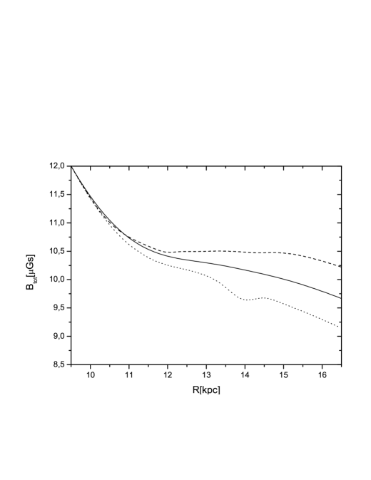
Figure 5: Comparison of the modelled magnetic field magnitudes that would account for the difference between the stellar rotation curve and three gaseous rotation curves obtained in cases when: 1) only the gas below the Galactic plane is considered (dashed line), 2) only the gas above the Galactic plane is considered (dotted line) and 3) when whole of the gas, that is, both below and above that plane is taken into account. The results were obtained assuming $h=4\,\mathrm{kpc}$.

In Fig.6 we compare (in units of speed) the contributions of magnetic terms present in the azimuthal part of equations Eq.3. The square root of Alfvén term $B_{\Phi}^{2}/4\pi\varrho$ (comparable with the Alfvén speed $\sqrt{\vec{B}\circ\vec{B}/4\pi\varrho}$ for the particular solution), grows with radius, reaching values comparable with the circular velocity of gas. The square root of absolute value of the gradient term $B_{\Phi}\partial_{R}B_{\Phi}/4\pi\varrho$, reaches values roughly twice lower, and depending on the sign, it increases or decreases the effect from the Alfvén term.

Figure 6: Comparison of magnetic terms in equation Eq.3a for a solution with $h=2\,\mathrm{kpc}$. Square root of Alfvén term $B_{\Phi}^{2}/4\pi\varrho$ [solid line], square root of absolute value of a gradient magnetic term $B_{\Phi}\partial_{R}B_{\Phi}/4\pi\varrho$ [dot line] (regions where this term is positive or negative are marked $+$ or $-$). The Alfvén speed $\sqrt{\vec{B}\circ\vec{B}/4\pi\varrho}$ [dashed line] is comparable in magnitude with the circular speed of gas [dash-dot line].

The radial velocity component $V_{R}$ can be obtained for the found solutions from Eq.3b. In Fig.7 the velocity is shown for a particular solution with $h=2\,\,\mathrm{kpc}$, however the velocity is almost the same for other $h$, the difference is noticeable only in the boundary region close to $R=9\,\mathrm{kpc}$.

Figure 7: Radial velocity component in Galactic magnetic field, estimated based on equation Eq.3b assuming $h=2\,\,\mathrm{kpc}$.

As we have seen earlier, the $V_{R}$ component can be interpreted in our model as a measure of the radial velocity dispersion due to the interaction with magnetic field that flops its radial direction, in which case the sign $V_{R}$ changes following these flops. The $V_{R}$ is of similar order of magnitude as the radial velocity dispersion observed for spiral galaxies, see Tamburro et al., [2009], what suggests that magnetic fields may be important in modeling the dispersion of gas. One can also use the $V_{R}$ component to estimate the accretion rate connected with the radial flow of gas. The accretion rate is defined in our case as the amount of matter flowing through a cylindric surface of radius $R$. Accordingly, using the density profile Eq.1, it can be estimated from $2\pi R\,\Sigma(R)V_{R}(R)$ or $8\pi R\,h\varrho(R,0)V_{R}(R)$. The resulting accretion rate for the same solution as above is shown in Fig.8, it will similarly be almost independent of $h$.

Figure 8: Accretion rate associated with the radial velocity component shown in Fig.7.

5 Conclusions

The difference between the stellar and gaseous rotation curves observed in the outer Galactic disc [Pont et al.,, 1997] is significant. Attributing it entirely to a magnetic interaction would require fields exceeding $10\,\mu\mathrm{G}$, strongly depending on the gas density in the Galactic disc. The question arises, whether fields of this magnitude could be present in the Galaxy. According to the interpretation sketched before, the ansatz Eq.4 for the magnetic field we assumed for solutions of the Navier-Stokes equations, takes into account the influence of the total magnetic field, including both the regular and turbulent magnetic components. It is important to note that the magnitude of the turbulent component in the Galaxy is not negligible, and may exceed the magnitude of the regular component. The regular field observed in the Galaxy is estimated to have a value of $5\,\mu\mathrm{G}$, while the turbulent field has $11\,\mu\mathrm{G}$ [Elstner et al.,, 2014]. Furthermore, Elstner et al., [2014] estimate, based on their models, that each of the components $B_{R}$, $B_{\Phi}$ and $B_{Z}$ of the total field may reach local values as high as $15\,\mu\mathrm{G}$ or more for lower radii, falling off with the radial distance, and exceeding $10\,\mu\mathrm{G}$, even at the radius of the solar orbit. Our results seem consistent with these findings.

For lower densities (higher scale parameters $h$), the magnetic field, as seen in Fig.4, is a decreasing function of radius, while for higher densities (corresponding to $h=2\,\,\mathrm{kpc}$, $1.5\,\,\mathrm{kpc}$ or lower) the field increases with radius or is approximately constant. Most often, the magnetic field is expected to decrease exponentially [Elstner et al.,, 2014], which may seem to disagree with our results at higher densities. Howewer, it should be remembered that the real density of HII regions, used to determine the gas rotation curve, may be lower than the density obtained for HI distribution. This is because ionized gas, such as in HII regions, should have lower density than the neutral hydrogen HI. If this was the case, the densities corresponding to higher $h$ (above $2\,\,\mathrm{kpc}$) would better approximate the density of the HII regions, which are influenced by magnetic fields. Then, the magnetic field found by us would have values and behaviour consistent with the usual assumptions.

Interestingly, we observed that Alfvén velocity reaches values comparable with the circular velocity of gas. Alfven velocities of more than $100\,\mathrm{km}/\mathrm{s}$ are about 10 times larger than the mid-plane turbulent velocity of $10\,\mathrm{km}/\mathrm{s}$. It means a $100$ times higher magnetic energy compared to the kinetic energy of the turbulence.

The volume gas density, important for the magnetic field determination, is strongly dependent on the assumed vertical profile of the gas layer. Fortunately, this uncertainty seems not so essential to the modelled magnetic field magnitudes required by the observed separation of stellar and gaseous rotation curves. This is so, because a higher volume density in the Galactic plane means a lower postulated scale height $h$, which in turn requires taking into account the altitudes of the HII regions used to determine the rotation curve of gas. The ionized hydrogen of HII regions is much more diluted than the neutral hydrogen of HI regions. Both kinds of gas, HI and HII, may belong to the same gas cloud which must move as a whole. It is therefore safer (in order not to reduce the magnetic field too much) to determine the (ionized) gas density such as if the gas consisted of HI hydrogen only. This approach overestimates the density of the ionized fraction.

As seen in Fig.5, the difference between circular velocities of gas in the northern and southern sides of the Galactic disc, if attributed to magnetic forces, requires small difference in the magnetic field magnitudes, not greater than $1.3\,\mu\mathrm{G}$. It is thus plausible that the difference in rotation may indeed be due to some asymmetry in the distribution of magnetic field.

To sum up: as the above magnetic field estimates show, it is plausible that most of the observed difference in the circular velocities of the stellar and gaseous fractions in the Galaxy may be caused by the presence of interstellar magnetic fields, frozen in the partially ionized gas, and holding the gaseous mass component together by the resulting magnetic tension. Within the possible range of higher densities corresponding to $h$ about $1-2\,\,\mathrm{kpc}$ or less, the magnetic field needs to increase with the distance (it is bound within $12$ and $16\,\,\mu\mathrm{G}$) or at least to be approximately constant between $10$ and $20\,\,\mathrm{kpc}$. Only for very low gas density at the Galactic plane, lower than $10^{-25}\,\mathrm{g}/\mathrm{cm}^{3}$, the magnetic field is decreasing with the Galactocentric distance, as observations suggest; the difference in rotation could be then explained by magnetic fields of order $10\,\,\mu\mathrm{G}$. If the real fields are different, then only a fraction of the rotation difference could be explained by the presence of magnetic fields. In any case, the difference in the rotation could be used as a means to estimate the intensity of the total magnetic field in spiral galaxies. This is also a manifestation of the influence of magnetic fields on the dynamics of spiral galaxies. Apart form the influence on the rotation, the radial component of magnetic field will modify the radial velocity dispersion.

References

- Battaner and Florido, [2007] Battaner, E. and Florido, E. (2007). Are rotation curves in NGC 6946 and the Milky Way magnetically supported? Astronomische Nachrichten, 328:92–98.
- Battaner et al., [2008] Battaner, E., Florido, E., Guijarro, A., Rubiño-Martín, J. A., and Ruíz-Granados, A. Z. (2008). Magnetic fields in Galaxies. Lecture Notes and Essays in Astrophysics, 3:83–102.
- Battaner et al., [1992] Battaner, E., Garrido, J. L., Membrado, M., and Florido, E. (1992). Magnetic fields as an alternative explanation for the rotation curves of spiral galaxies. Nature, 360:652.
- Battinelli et al., [2013] Battinelli, P., Demers*, S., Rossi**, C., and Gigoyan, K. S. (2013). Extension of the C Star Rotation Curve of the Milky Way to 24 kpc. Astrophysics, 56:68–75.
- Berdnikov et al., [2000] Berdnikov, L. N., Dambis, A. K., and Vozyakova, O. V. (2000). Galactic Cepheids. Catalogue of light-curve parameters and distances. A&AS, 143:211–213.
- Blitz et al., [1982] Blitz, L., Fich, M., and Stark, A. A. (1982). Catalog of CO radial velocities toward galactic H II regions. ApJS, 49:183–206.
- Brand and Blitz, [1993] Brand, J. and Blitz, L. (1993). The Velocity Field of the Outer Galaxy. A&A, 275:67.
- Caldwell and Coulson, [1987] Caldwell, J. A. R. and Coulson, I. M. (1987). Milky Way rotation and the distance to the galactic center from Cepheid variables. AJ, 93:1090–1105.
- Chini and Wink, [1984] Chini, R. and Wink, J. E. (1984). The galactic rotation outside the solar circle. A&A, 139:L5–L8.
- Clemens, [1985] Clemens, D. P. (1985). Massachusetts-Stony Brook Galactic plane CO survey - The Galactic disk rotation curve. ApJ, 295:422–428.
- Demers and Battinelli, [2007] Demers, S. and Battinelli, P. (2007). C stars as kinematic probes of the Milky Way disk from 9 to 15 kpc. A&A, 473:143–148.
- Elstner et al., [2014] Elstner, D., Beck, R., and Gressel, O. (2014). Do magnetic fields influence gas rotation in galaxies? A&A, 568:A104.
- Fich et al., [1989] Fich, M., Blitz, L., and Stark, A. A. (1989). The rotation curve of the Milky Way to 2 R(0). ApJ, 342:272–284.
- [14] Jałocha, J., Bratek, Ł., Pȩkala, J., and Kutschera, M. (2012a). A possible influence of magnetic fields on the rotation of gas in NGC 253. MNRAS, 427:393–396.
- [15] Jałocha, J., Bratek, Ł., Pȩkala, J., and Kutschera, M. (2012b). The role of large-scale magnetic fields in galaxy NGC 891: can magnetic fields help to reduce the local mass-to-light ratio in the galactic outskirts? MNRAS, 421:2155–2160.
- Kalberla et al., [2007] Kalberla, P. M. W., Dedes, L., Kerp, J., and Haud, U. (2007). Dark matter in the Milky Way. II. The HI gas distribution as a tracer of the gravitational potential. A&A, 469:511–527.
- Kalberla and Kerp, [2009] Kalberla, P. M. W. and Kerp, J. (2009). The Hi Distribution of the Milky Way. ARA&A, 47:27–61.
- Kutschera and Jałocha, [2004] Kutschera, M. and Jałocha, J. (2004). Rotation Curves of Spiral Galaxies: Influence of Magnetic Fields and Energy Flows. Acta Physica Polonica B, 35:2493.
- Levine et al., [2006] Levine, E. S., Blitz, L., and Heiles, C. (2006). The Vertical Structure of the Outer Milky Way H I Disk. ApJ, 643:881–896.
- May et al., [1997] May, J., Alvarez, H., and Bronfman, L. (1997). Physical properties of molecular clouds in the southern outer Galaxy. A&A, 327:325–332.
- Mel’nik et al., [2015] Mel’nik, A. M., Rautiainen, P., Berdnikov, L. N., Dambis, A. K., and Rastorguev, A. S. (2015). Classical Cepheids in the Galactic outer ring R_1R_2’. Astronomische Nachrichten, 336:70.
- Nakanishi and Sofue, [2006] Nakanishi, H. and Sofue, Y. (2006). Three-Dimensional Distribution of the ISM in the Milky Way Galaxy: II. The Molecular Gas Disk. PASJ, 58:847–860.
- Nakanishi and Sofue, [2016] Nakanishi, H. and Sofue, Y. (2016). Three-dimensional distribution of the ISM in the Milky Way galaxy. III. The total neutral gas disk. PASJ, 68:5.
- Pont et al., [1994] Pont, F., Mayor, M., and Burki, G. (1994). New radial velocities for classical cepheids. Local galactic rotation revisited. A&A, 285.
- Pont et al., [1997] Pont, F., Queloz, D., Bratschi, P., and Mayor, M. (1997). Rotation of the outer disc from classical cepheids. A&A, 318:416–428.
- Ruiz-Granados et al., [2012] Ruiz-Granados, B., Battaner, E., Calvo, J., Florido, E., and Rubiño-Martín, J. A. (2012). Dark Matter, Magnetic Fields, and the Rotation Curve of the Milky Way. ApJL, 755:L23.
- [27] Ruiz-Granados, B., Rubiño-Martín, J. A., and Battaner, E. (2010a). Constraining the regular Galactic magnetic field with the 5-year WMAP polarization measurements at 22 GHz. A&A, 522:A73.
- [28] Ruiz-Granados, B., Rubiño-Martín, J. A., Florido, E., and Battaner, E. (2010b). Magnetic Fields and the Outer Rotation Curve of M31. ApJL, 723:L44–L48.
- Sánchez-Salcedo and Santillán, [2013] Sánchez-Salcedo, F. J. and Santillán, A. (2013). Magnetic fields: impact on the rotation curve of the Galaxy. MNRAS, 433:2172–2181.
- Tamburro et al., [2009] Tamburro, D., Rix, H.-W., Leroy, A. K., Mac Low, M.-M., Walter, F., Kennicutt, R. C., Brinks, E., and de Blok, W. J. G. (2009). What is Driving the H I Velocity Dispersion? AJ, 137:4424–4435.
- Vallee, [1991] Vallee, J. P. (1991). Reversing the axisymmetric (m = 0) magnetic fields in the Milky Way. ApJ, 366:450–454.