Nonconvex penalized multitask regression using data depth-based penalties

Abstract

We propose a new class of nonconvex penalty functions, based on data depth functions, for multitask sparse penalized regression. These penalties quantify the relative position of rows of the coefficient matrix from a fixed distribution centered at the origin. We derive the theoretical properties of an approximate one-step sparse estimator of the coefficient matrix using local linear approximation of the penalty function, and provide algorithm for its computation. For orthogonal design and independent responses, the resulting thresholding rule enjoys near-minimax optimal risk performance, similar to the adaptive lasso (Zou, 2006). A simulation study and real data analysis demonstrate its effectiveness compared to some of the present methods that provide sparse solutions in multivariate regression.

Keywords: Multitask regression; Nonconvex penalties; Sparsity; Data depth

1 Introduction

Consider the multitask linear regression model:

$$Y=XB+E$$

where $Y\in\mathbb{R}^{n\times q}$ is the matrix of responses, and $E$ is $n\times q$ the noise matrix: each row of which is drawn from $\mathcal{N}_{q}(0,\Sigma)$ for a $q\times q$ positive definite matrix $\Sigma$. We are interested in sparse estimates of the coefficient matrix $B\in\mathbb{R}^{p\times q}$, which are useful for inference in regression problems with a large number of predictors that have differential influences on multiple correlated response variables: for example in gene-expression data (Lozano and Świrszcz, 2012; Molstad and Rothman, 2016) and prediction of stock returns (Rothman et al., 2010). This is done through solving penalized regression problems of the form

$$\min_{B}\operatorname*{Tr}\{(Y-XB)^{T}(Y-XB)\}+P_{\lambda}(B)$$ (1.1)

The frequently studied single-response linear model may be realized as a special case of this with $q=1$. In this setup, obtaining sparse estimates of the coefficient vector $\beta$ involves solving an optimization problem with the penalty function $P(\beta)=\sum_{j=1}^{p}p(|\beta_{j}|)$:

$$\hat{\beta}_{n}=\operatorname*{arg\,min}_{\beta}\left[\sum_{i=1}^{n}\rho(y_{i}-X_{i}^{T}\beta)+\lambda_{n}\sum_{j=1}^{p}p(|\beta_{j}|)\right]$$ (1.2)

for a general loss function $\rho(.)$, with $\lambda_{n}$ being a tuning parameter depending on sample size. The penalty term is generally a measure of model complexity that controls for overfitting. Starting from LASSO (Tibshirani, 1996) which uses the $l_{1}$ norm, i.e. $p(z)=|z|$, relevant methods in this domain include adaptive LASSO (Zou, 2006) that reweights the coordinate-wise LASSO penalties based on the Ordinary Least Square (OLS) estimate of $\beta$, and non-convex penalties proposed by Fan and Li (2001) and Zhang (2010) that limit influence of large entries in the coefficient vector $\beta$, resulting in improved estimation of $\beta$. Further, Zou and Li (2008) and Wang et al. (2013) provided efficient algorithms for computing solutions to the nonconvex penalized problems.

For multiple responses, Rothman et al. (2010) showed that penalizing at the coefficient matrix-level results in better estimation and prediction performance compared to performing $q$ separate LASSO regressions. Here the coefficient matrix $B$ has two levels of sparsity. The first level is recovering the set of predictors having non-zero effects on all the responses, while the second level of sparsity is concerned with recovering non-zero elements within the non-zero rows obtained from the first step. Previous studies have performed this using either a bi-level penalty function (Vincent and Hansen, 2014; Li et al., 2015) or a group lasso penalization to recover non-zero rows followed by within-row thresholding (Obozinski et al., 2011).

In this paper, we introduce a class of non-convex penalty functions of the form $P(B)=\sum_{j=1}^{p}\lambda p(b_{j})$, $b_{j}$ being the $j$-th row of $B$, in multitask regression. We use data depth functions (Zuo and Serfling, 2000) to construct our row-level penalties, which quantify the relative position of $b_{j}$ with respect to a fixed probability distribution centered at the origin. We approximate this penalty function using local linear approximation, obtain a first level row-sparse estimate, and recover within-row non-zero elements of $B$ through a corrective thresholding of this estimate. When the design matrix is orthogonal and responses independent, the thresholding rule resulting from our proposed penalty has asymptotically optimal minimax risk. Finally we demonstrate the performance of our method relative to some alternatives through a simulation study and microarray data analysis. The supplementary material contains proofs of theoretical results, and additional simulations.

2 Depth-based regularization

2.1 Data depth

Given a data cloud or a probability distribution, a depth function is any real-valued function that measures the outlyingness of a point in feature space with respect to the data or its underlying distribution (figure 1 panel a). In order to formalize the notion of depth, we consider as data depth any scalar-valued function $D(x,F_{X})$ (where $x\in\mathbb{R}^{p}$, and the random variable $X$ has distribution $F_{X}$) that satisfies the following properties (Liu, 1990):

(P1) Affine invariance: $D(Ax+b,F_{AX+b})=D(x,F_{X})$ for any $p\times p$ non-singular matrix $A$ and $p\times 1$ vector $b$;

(P2) Maximality at center: When $F_{X}$ has center of symmetry $\theta$, $D(\theta,F_{X})=\sup_{x\in\mathbb{R}^{p}}D(x,F_{X})$. Here the symmetry can be central, angular or halfspace symmetry;

(P3) Monotonicity relative to deepest point: For any $p\times 1$ vector $x$ and $\alpha\in[0,1]$, $D(x,F_{X})\leq D(\theta+a(x-\theta))$;

(P4) Vanishing at infinity: As $\|x\|\rightarrow\infty$, $D(x,F_{X})\rightarrow 0$.

Examples of data depth include halfspace depth (Tukey, 1975) and projection depth (Zuo, 2003). Data depth has been a popular tool for robust nonparametric and functional inference in the past two decades (Jornsten, 2004; Zuo et al., 2004; Zuo and Cui, 2005; Narisetty and Nair, 2016).

2.2 Motivation

Given a measure of data depth $D(.,.)$, we define any nonnegative-valued, bounded monotonically decreasing one-to-one transformation on that depth function as an inverse depth function, and denote it by $D^{-}(.,.)$. Some examples of inverse depth transformations include but are not limited to $D^{-}(x,F_{X}):=\max_{x}D(x,F_{X})-D(x,F_{X})$ and $D^{-}(x,F_{X}):=\exp(-D(x,F_{X}))$. We incorporate inverse depths as row-level penalty functions in (1.1). Specifically, we estimate $B$ by solving the following constrained optimization problem:

$$\hat{B}=\operatorname*{arg\,min}_{B}\left[\operatorname*{Tr}\{(Y-XB)^{T}(Y-XB)\}+\lambda_{n}\sum_{j=1}^{p}D^{-}(b_{j},F)\right]$$ (2.1)

We refer to $F$ as the reference distribution, and consider it fixed in the estimation process.

In multitask regression, any additive penalty function of the form $P_{\lambda}(B)=\sum_{j=1}^{p}\lambda p(b_{j})$ regularizes individual rows of the coefficient matrix by providing a control over their distance from the $q$-dimensional origin through some norm (e.g. the $l_{1}/l_{q}$ penalty: Neghaban and Wainwright (2011)), or a combination of norms (e.g. the Adaptive Multi-task Elastic-Net: Chen et al. (2012)). Through (2.1) we generalize this notion by proposing to regularize using the ‘distance’ from a probability distribution centered at the origin. Any existing method of norm-based regularization arises as a special case by by using the norm (or combination of norms) as the inverse depth function and taking the degenerate distribution centered at $0$ as $F$ .

Inverse depth functions essentially invert the funnel-shaped contour of the corresponding depth function (panel a of Figure 1). This immediately results in row-wise nonconvex penalties, where the penalty sharply increases for smaller entries inside the row but is bounded above for large values (see the case for $p=1$ in panel b of Figure 1). This serves as our motivation of using data depth in regularized multitask regression.

3 The LARN algorithm

3.1 Formulation

The reference distribution $F$ is pivotal in the estimation problem in (2.1). While we think that there is scope for a significant amount of theoretical analysis on the implications of different choices of $F$ and its potential connections to Bayesian regularized support union recovery in multitask regression (Chen et al., 2014), here we shall work within a simplified setup. Specifically we assume that

(A1) The distribution $F$ is spherically symmetric.

This is a fair assumption to make from a frequentist perspective, as we do not possess any extra information about the $q$ responses being different from one another. Since $F$ is spherically symmetric, depth at a point $b$ becomes a function of $r=\|b\|_{2}$ only, due to the affine invariance of $D(.,F)$. In this situation, several depth functions have closed-form expressions: e.g. when $D$ is projection depth and $F$ is a $p$-variate standard normal distribution, $D(b_{j},F)=c/(c+r_{j});c=\Phi^{-1}(3/4)$ (Zuo, 2003), while for halfspace depth and any known $F$, $D(b_{j},F)=1-F_{1}(r_{j})$, $F_{1}$ being any univariate marginal of $F$ (immediate from the definition of halfspace depth) and $r_{j}=\|b_{j}\|_{2}$. Hence, the computational burden of calculating depths for rows of $B$ becomes trivial.

Figure 1: (a) Contour plot of data depths for 500 points drawn form ${\cal{N}}_{2}(0,\operatorname*{diag}(2,1))$; (b) Comparison of L1 and SCAD (Fan and Li, 2001) penalty functions with univariate halfspace depth: inverting the depth function helps obtain the nonconvex shape of the penalty function in the inverse depth; (c) Univariate thresholding rule for the LARN estimate assuming halfspace depth and max definition of inverse depth (see Section 4)

Because of the way we define inverse depth functions, the above holds for inverse depth functions $D^{-}(.,F)$ as well. Thus we can write that $D^{-}(b_{j},F)=p_{F}(r_{j}),r_{j}=\|b_{j}\|_{2}$ for some scalar-valued function $p_{F}(.)$. Any superscript or subscript in $B$ or $b_{j}$ will be passed accordingly to $r_{j}$. At this point we make another assumption on $p_{F}(.)$:

(A2) The function $p_{F}(r)$ is concave in $r$, and continuously differentiable at every $r\neq 0$.

In general depth functions are assumed to have convex contours (Mosler, 2013), which implies quasi-concavity. Nevertheless, several depth functions adhere to concavity owing to their simplified closed forms for spherical distributions (e.g. halfspace depth and projection depth as stated earlier). Continuous differentiability except at the origin, which is essential for admitting a sparse solution to (2.1), arises because of the same reason.

Keeping the above setup in mind, we consider the first-order Taylor series approximation of the overall penalty function:

$$P_{\lambda.F}(B) = \lambda\sum_{j=1}^{p}p_{F}(r_{j})$$ (3.1)

$$\simeq \lambda\sum_{j=1}^{p}\left[p_{F}(r_{j}^{*})+p^{\prime}_{F}(r_{j}^{*})(r_{j}-r_{j}^{*})\right]$$

for any $B^{*}$ close to $B$, and $r_{j}=\|b_{j}\|_{2},r_{j}^{*}=\|b_{j}^{*}\|_{2};j=1,2,...,p$.

Given a starting solution $B^{*}$ close enough to the original coefficient matrix, $P_{\lambda.F}(B)$ is approximated by its conditional counterpart, say $P_{\lambda.F}(B|B^{*})$. Following this a penalized maximum likelihood estimate for $B$ can be obtained using the iterative algorithm below:

1. Take as starting value $B^{(0)}=\hat{B}_{\text{LS}}=(X^{T}X)^{-}X^{T}Y$, i.e. the least square estimate of $B$, set $k=0$;

2. Calculate the next iterate by solving the penalized likelihood:

   $$B^{(k+1)}=\operatorname*{arg\,min}_{B}\left[\operatorname*{Tr}\left\{(Y-XB^{(k)})^{T}(Y-XB^{(k)})\right\}+\lambda\sum_{j=1}^{p}p^{\prime}_{F}(r_{j}^{(k)})r_{j}\right]$$ (3.2)

3. Continue until convergence.

Taking $\hat{B}_{\text{LS}}$ as a starting value ensures that $\|\hat{B}_{\text{LS}}-B\|_{F}=O(n^{-1/2})$ given the data, hence we get from (3.1) that

$$P_{\lambda,F}(B)=P_{\lambda,F}(B|\hat{B}_{\text{LS}})+\sum_{j=1}^{p}o(|r_{j}-\hat{r}_{j,\text{LS}}|)=P_{\lambda,F}(B|\hat{B}_{\text{LS}})+o(n^{-1/2})$$

for fixed $p$. This algorithm approximates contours of the nonconvex penalty function using gradient planes at successive iterates, and is a multivariate generalization of the local linear approximation algorithm of Zou and Li (2008). We call this the Local Approximation by Row-wise Norm (LARN) algorithm.

LARN is a majorize-minimize (MM) algorithm where the actual objective function $Q(B)$ is being majorized by $R(B|B^{(k)})$, with

$$Q(B) =\operatorname*{Tr}\left\{(Y-XB)^{T}(Y-XB)\right\}+P_{\lambda,F}(B)$$

$$R(B|B^{(k)}) =\operatorname*{Tr}\left\{(Y-XB)^{T}(Y-XB)\right\}+P_{\lambda,F}(B|B^{(k)})$$

This is easy to see, because $Q(B)-R(B|B^{(k)})$ = $\lambda\sum_{j=1}^{p}\left[p_{F}(r_{j})-p_{F}(r_{j}^{*})-p^{\prime}_{F}(r_{j}^{*})(r_{j}-r_{j}^{*})\right]$. And since $p_{F}(.)$ is concave in its argument, we have $p_{F}(r_{j})\leq p_{F}(r_{j}^{*})+p^{\prime}_{F}(r_{j}^{*})(r_{j}-r_{j}^{*})$. Thus $Q(B^{(k)})\leq R(B|B^{(k)})$. Also by definition $Q(B)=R(B^{(k)}|B^{(k)})$.

Now notice that $B^{(k+1)}=\operatorname*{arg\,min}_{B}R(B|B^{(k)})$. Thus $Q(B^{(k+1)})\leq R(B^{(k+1)}|B^{(k)})\leq R(B^{(k)}|B^{(k)})=Q(B^{(k)})$, i.e. the value of the objective function decreases in each iteration. At this point, we make the following assumption to enforce convergence to a local solution:

(A3) $Q(B)=Q(M(B))$ only for stationary points of $Q$, where $M$ is the mapping from $B^{(k)}$ to $B^{(k+1)}$ defined in 3.2.

Since the sequence of penalized losses i.e. $\{Q(B^{(k)}\}$ is bounded below (by 0) and monotone, it has a limit point, say $\hat{B}$. Also the mapping $M(.)$ is continuous as $\nabla p_{F}$ is continuous. Further, we have $Q(B^{(k+1)})=Q(M(B^{(k)}))\leq Q(B^{(k)})$ which implies $Q(M(\hat{B}))=Q(\hat{B})$. It follows that $\hat{B}$ is a stationary point following assumption (A3).

Remark. Although the LARN algorithm guarantees convergence to a stationary point, that point may not be a local solution. However, local linear approximation has been found to be effective in approximating nonconvex penalties and obtaining oracle solutions for single-response regression (Zou and Li, 2008) and support vector machines (Peng et al., 2016). We generalize this concept for the multitask situation.

3.2 The one-step estimate and its oracle properties

Due to the row-wise additive structure of our penalty function, supports of each of the iterates $\hat{B}^{(k)}$ in the LARN algorithm have the same set of singular points as the solution to the original optimization problem, say $\hat{B}$. Consequently all iterates are capable of producing sparse solutions. In fact, the first iterate itself possesses oracle properties desirable of row-sparse estimates, namely consistent recovery of the non-zero row support of $B$, as well as of the elements in those rows. This is in line with the findings of Zou and Li (2008) and Fan and Chen (1999).

Given an initial solution $B^{*}$, the first LARN iterate, say $\hat{B}^{(1)}$, is a solution to the optimization problem:

$$\operatorname*{arg\,min}_{B}R(B|B^{*}) = \operatorname*{arg\,min}_{B}\left[\operatorname*{Tr}\left\{(Y-XB)^{T}(Y-XB)\right\}+\lambda\sum_{j=1}^{p}p^{\prime}_{F}(r_{j}^{(k)})r_{j}\right]$$ (3.3)

At this point, without loss of generality we assume that the true coefficient matrix $B$ has the following decomposition: $B_{0}=(B^{T}_{01},0)^{T},B_{1}\in\mathbb{R}^{p_{1}\times q},0<p_{1}<p$. Also denote the vectorized (i.e. stacked-column) version of a matrix $A$ by $\text{vec}(A)$. We are now in a position to to prove oracle properties of the one-step estimator in (3.3), in the sense that the estimator is able to consistently detect zero rows of $B$ as well as estimate its non-zero rows as sample size increases:

Theorem 3.1.

Assume that $X^{T}X/n\rightarrow C$ for some positive definite matrix $C$, and $p^{\prime}_{F}(r_{j}^{*})=O((r_{j}^{*})^{-s})$ for $1\leq j\leq q,0<r_{j}^{*}<\delta$ and some $s>0,\delta>0$. Consider a sequence of tuning parameters $\lambda_{n}$ such that $\lambda_{n}/\sqrt{n}\rightarrow 0$ and $\lambda_{n}n^{(s-1)/2}\rightarrow\infty$. Then the following holds for the one-step estimate $\hat{B}^{(1)}=(\hat{B}^{T}_{11},\hat{B}^{T}_{10})^{T}$ (with the component matrices having dimensions $p_{1}\times q$ and $p-p_{1}\times q$, respectively) as $n\rightarrow\infty$:

(1) $\operatorname*{vec}(\hat{B}_{10})\rightarrow 0$ in probability;

(2) $\sqrt{n}(\operatorname*{vec}(\hat{B}_{11})-\operatorname*{vec}(B_{01}))\leadsto\mathcal{N}_{p_{1}q}(0,\Sigma\otimes C_{11}^{-1})$

where $C_{11}$ is the first $p_{1}\times p_{1}$ block in $C$.

The assumption on $X$ is standard, and ensures uniqueness of the asymptotic covariance matrix of our estimator. The restricted eigenvalue condition, which has been used to establish finite sample error bounds of penalized estimators (Neghaban et al., 2009) is a stronger version of this. With respect to the general framework of nonconvex penalized $M$-estimation in Loh and Wainwright (2015), $p_{F}(.)$ satisfies parts (i)-(iv) of Assumption 1 therein, and the conditions of theorem 3.1 adhere to part (v).

Remark. The above oracle results depend on the assumption (A1), which simplifies depth as a function of the row-norm. We conjecture that similar oracle properties hold for weaker assumptions. From initial attempts into proving a broader result, we think it requires a more complex approach than the proof of Theorem 3.1.

3.3 Recovering sparsity within a row

The set of variables with non-zero coefficients for each of the $q$ univariate regressions may not be the same, hence recovering non-zero elements within the rows is of interest as well. It turns out that consistent recovery at this level can be achieved by simply thresholding elements of the non-zero elements in the one-step estimate obtained in the preceding subsection. Obozinski et al. (2011) have shown that a similar approach recovers within-row supports in multivariate group lasso. The following result formalizes this in our scenario, provided that non-zero signals in $B$ are large enough:

Lemma 3.2.

Suppose the conditions of theorem 3.1 hold, and additionally all non-zero components of $B$ have the following lower bound:

$$|b_{jk}|\geq\sqrt{\frac{16\log(qp_{1})}{C_{min}n}};\quad 1\leq j\leq p_{1},1\leq k\leq q$$

where $C_{\min}>0$ is a lower bound for eigenvalues of $C_{11}$. Also define by $\hat{\cal{S}}$ the index set of non-zero rows estimated by the LARN algorithm. Then, for some constants $c,c_{0}>0$, the post-thresdolding estimator $T(\hat{B}^{(1)})$ defined by:

$$t_{jk}=\begin{cases}0&\text{ if }\hat{b}_{jk}^{(1)}\leq\sqrt{\frac{8\log(q|\hat{\cal{S}}|)}{C_{min}n}}\\ \hat{b}_{jk}^{(1)}&\text{ otherwise }\end{cases};\quad j\in\hat{\cal{S}},1\leq k\leq q$$

has the same set of non-zero supports within rows as $B$ with probability greater than $1-c_{0}\exp(-cq\log p_{1})$.

3.4 Computation

When $B$ and $Y-XB$ are replaced with their corresponding vectorized versions, the optimization problem in (3.3) reduces to a weighted group lasso (Yang and Zou, 2015) setup, with group norms corresponding to $l^{2}$ norms of rows of $B$ and inverse depths of corresponding rows of the initial estimate $B^{*}$ acting as group weights. To compute a solution here, we start from the following lemma, which gives necessary and sufficient conditions for the existence of a solution:

Lemma 3.3.

Given an initial value $B^{*}$, a matrix $B\in\mathbb{R}^{p\times q}$ is a solution to the optimization problem in (3.3) if and only if:

1. $2x_{j}^{T}(Y-XB)+\lambda p^{\prime}_{F}(r_{j}^{*})b_{j}/r_{j}=0$ if $b_{j}\neq 0$;

2. $\|x_{j}^{T}(Y-XB)\|_{2}\leq\lambda/2$ if $b_{j}=0$.

This lemma is a modified version of lemma 4.2 in chapter 4 of Buhlmann and van de Geer (2011), and can be proved in a similar fashion. Following the lemma, we use a block coordinate descent algorithm (Li et al., 2015) to iteratively compute $\hat{B}^{(1)}$.

We use $k$-fold cross-validation to choose the optimal $\lambda$. Additionally, in a sample setup the quantity $C_{\text{min}}$ in Lemma 3.2 is unknown, so we choose a best threshold for within-row sparsity through cross-validation as well. Even though this means that the cross-validation has to be done over a two-dimensional grid, the thresholding step is actually done after estimation. Thus for any fixed $\lambda$, only $k$ models need to be calculated. Given a trained model for some value of $\lambda$ we just cycle through the full range of thresholds to record their corresponding cross-validation errors.

4 Orthogonal design and independent responses

We shed light on the workings of our penalty function by considering the simplified scenario when the predictor matrix $X$ is orthogonal and all responses are independent. Independent responses make minimizing (2.1) equivalent to solving of $q$ separate nonconvex penalized regression problems, while orthogonal predictors make the LARN estimate equivalent to a collection of coordinate-wise soft thresholding operators.

4.1 Thresholding rule

For the univariate thresholding rule, we are dealing with the simplified penalty function $p_{F}(|b_{jk}|)=D^{-}(b_{jk},F)$, where $D^{-}$ is a inverse depth function based on the univariate depth function $D$. In this case, depth calculation becomes simplified in exactly the same way as in Subsection 3.1, only $|b_{jk}|$ replacing $\|b_{j}\|_{2}$ therein, and $1\leq k\leq q$.

Following Fan and Li (2001), a sufficient condition for the minimizer of the penalized least squares loss function

$$L(\theta;p_{\lambda})=\frac{1}{2}(z-\theta)^{2}+p_{\lambda}(|\theta|)$$ (4.1)

to be unbiased when the true parameter value is large is $p^{\prime}_{\lambda}(|\theta|)=0$ for large $\theta$. In our formulation, this holds exactly when $F$ has finite support, and approximately otherwise. A necessary condition for sparsity and continuity of the solution is $\min_{\theta\neq 0}|\theta|+p^{\prime}_{\lambda}(|\theta|)>0$. We ensure this by making a small assumption about the derivative of $D^{-}$ (denoted by $D^{-}_{1})$:

(A4) $\lim_{\theta\rightarrow 0+}D^{-}_{1}(\theta,F)>0$.

Subsequently we get the following thresholding rule as the solution to (4.1):

$$\hat{\theta}(F,\lambda) = \text{sign}(z)\left[|z|-\lambda D^{-}_{1}(\theta,F)\right]_{+}$$ (4.2)

$$\simeq \text{sign}(z)\left[|z|-\lambda D^{-}_{1}(z,F)\right]_{+}$$

The approximation in the second step above is due to Antoniadis and Fan (2001). A plot of the thresholding function in panel c of Figure 1 demonstrates the unbiasedness and continuity properties of this estimator.

Thresholding rules due to previously proposed nonconvex penalty functions arise as special cases of our rule. For example, when we use halfspace depth and the max definition of inverse depth, i.e. $D^{-}(b,F)=\max_{x}D^{-}(x,F)-D^{-}(b,F)$, the MCP penalty (Zhang, 2010) corresponds to $D^{-}_{1}(\theta,F)=|\theta|{\mathbb{I}}_{|\theta|<\lambda}$, while for the SCAD penalty (Fan and Li, 2001):

$$D^{-}_{1}(\theta,F)=\begin{cases}c\lambda&\text{ if }|\theta|<2\lambda\\ \frac{c}{a-2}(a\lambda-|\theta|)&\text{ if }2\lambda\leq|\theta|<a\lambda\\ 0&\text{ if }|\theta|>a\lambda\end{cases}$$

with $c=1/(2\lambda^{2}(a+2))$.

4.2 Minimax optimal performance

In the context of estimating the mean parameters $\mu_{i}$ of independent and identically distributed observations with normal errors: $z_{i}=\theta_{i}+v_{i},v_{i}\sim N(0,1)$, the minimax risk is $2\log n$ times the ideal risk $R(\text{ideal})=\sum_{i=1}^{n}\min(\theta_{i}^{2},1)$ (Donoho and Johnstone, 1994). A major motivation of using lasso-type penalized estimators in linear regression is that they are able to approximately achieve this risk bound for large sample sizes (Donoho and Johnstone, 1994; Zou, 2006). We now show that our thresholding rule in (4.2) also replicates this performance.

Theorem 4.1.

Suppose the inverse depth function $D^{-}(.,F)$ is twice continuously differentiable, except at the origin, with first and second derivatives bounded above by $c_{1}$ and $c_{2}$ respectively. Then for $\lambda=(\sqrt{.5\log n}-1)/c_{1}$, we have

$$R(\hat{\theta}(F,\lambda)) \leq (2\log n-3)\left[R(ideal)+\frac{c_{1}}{p_{0}(F)(\sqrt{.5\log n}-1)}\right]$$ (4.3)

with $p_{0}(F)=\lim_{\theta\rightarrow 0+}D^{-}_{1}(\theta,F)$.

Following the theorem, we easily see that for large $n$ the minimax risk of $\hat{\theta}(F,\lambda)$ approximately achieves the $2\log n$ multiple bound.

The adaptive lasso (Zou, 2006) guarantees a similar minimax risk bound in single-response regression. This is somewhat expected, given the similar weighted norm structure of the LARN penalty and the adaptive lasso penalty. However, this does not hold for all weighted norm penalties: for example the SCAD and MCP penalties do not ensure near-minimax optimal performance because of their non-continuity in the second derivative. In this situation, using inverse depth functions that satisfy all the conditions in the theorem (both halfspace depth and projection depth do because of the simplification in Subsection 3.1) allows us to go through with the result.

5 Simulation results

5.1 Methods and setup

We use the setup of Rothman et al. (2010) in a simulation study to compare the performance of LARN with other relevant methods. Specifically, we use performance metrics calculated after applying the following methods of predictor selection on simulated data for this purpose:

LARN: We use halfspace depth as our chosen depth function and take $D^{-}(x,F)=\max_{x}D(x,F)-D(x,F)$;

Thresholded Group Lasso (TGL: Obozinski et al. (2011)): Performs element-wise thresholding on a row-level group lasso estimator to get final estimate of $B$. It is a special case of LARN, with weights of all row-norms set to 1;

Sparse Group Lasso (SGL: Vincent and Hansen (2014)): This method recovers within row sparsity by considering an $l_{1}$ penalty over individual elements of $B$ in addition to the $l_{1}/l_{2}$ row-level penalties. We use the R package lsgl to fit the model;

Separate Lasso: We train separate lasso models on all response variables with a common tuning parameter.

For all the methods above, we use 5-fold cross-validation on a 100-length sequence of numbers between $(-2,2)$ as the set of tuning parameters in the respective optimization algorithms. Additionally for LARN and TGL, we use a 100-length sequence between (0, $0.9\max|\hat{B}^{(1)}|$) as the set of tuning parameters for within-row thresholding of the first-step estimator $\hat{B}^{(1)}$.

We generate rows of the model matrix $X$ as $n=50$ independent draws from $\mathcal{N}(0,\Sigma_{X})$, where the positive definite matrix $\Sigma_{X}$ has a first-order autoregressive (AR(1)) covariance structure, with its $(i,j)^{\text{th}}$ element given by $0.7^{|i-j|}$. We generate rows of the random error matrix $E$ as independent draws from $\mathcal{N}(0,\Sigma)$: with $\Sigma$ also having an AR(1) structure with correlation parameter $\rho\in\{0,0.5,0.7,0.9\}$. Finally, to generate the coefficient matrix $B_{0}$, we obtain the three $p\times q$ matrices: $W$, whose elements are independent draws from $N(2,1)$; $K$, which has elements as independent draws from Bernoulli$(0.3)$; and $Q$ whose rows are made all 0 or all 1 according to $p$ independent draws of another Bernoulli random variable with success probability $0.125$. Following this, we multiply individual elements of these matrices (denoted by $(*)$) to obtain a sparse $B_{0}$:

$$B_{0}=W*K*Q$$

Notice that the two levels of sparsity we consider: entire row and within-row, are imposed by the matrices $Q$ and $K$, respectively.

For a given value of $\rho$, we consider three settings of data dimensions for the simulations: (a) $p=20,q=20$, (b) $p=20,q=60$, (c) $p=60,q=60$ and (d) $p=100,q=60$. Finally we replicate the full simulation 100 times for each set of $(p,q,\rho)$. For brevity, we report only the results for $\rho=0.7$ here, and provide those for $\rho=0$, $\rho=0.5$ and $\rho=0.9$ in the supplementary material.

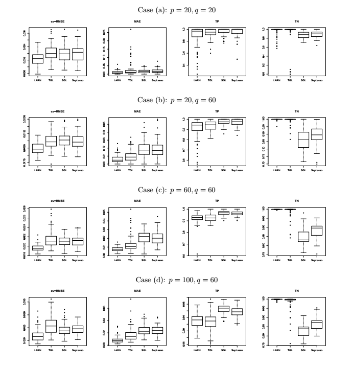
Figure 2: Boxplots of evaluation metrics for all methods in different $(p,q)$ settings: $\rho=0.7$.

Figure 3: Estimated effects of Mevalonate pathway genes (rows) on the activity of non-mevalonate pathway genes (columns) in A. thaliana. Green/ red indicate positive/ negative values. Genes were ordered using hierarchical clustering.

5.2 Evaluation

To summarize the performance of an estimate matrix $\hat{B}$ we use the following three performance metrics:

Cross-validated Root Mean Squared Error (cv-RMSE)- Defined as

$$\text{cv-RMSE}(\hat{B})=\frac{1}{nq}\sqrt{\sum_{k=1}^{K}\text{Tr}\left[(Y_{k}-X_{k}\hat{B}_{-k})(Y_{k}-X_{k}\hat{B}_{-k})^{T}\right]}$$

for a dataset split into $K$ folds. Here$(Y_{k},X_{k})$ are the data for samples in the $k$-th fold, and $\hat{B}_{-k}$ is the estimate obtained from a model trained on samples outside the $k$-th fold;

Mean Absolute Error (MAE): Defined as the mean absolute value of entries in $\hat{B}-B_{0}$;

True Positive Rate (TP) - The proportion of non-zero entries in $B_{0}$ detected as non-zero in $\hat{B}$;

True Negative Rate (TN) - The proportion of zero entries in $B_{0}$ detected as zero in $\hat{B}$.

A desirable estimate shall have high TP and TN proportions, and low average cv-RMSE and MAE. We summarize the performances of all four methods in Figure 2. LARN and TGL outperform the other two methods handsomely in all cases. Although their TP and TN performances are similar, LARN estimates perform better in out-of-sample prediction and estimastion of elements in $B$ compared to TGL, owing to lesser cv-RMSE and MAE values. This is expected because the weighted penalties provide asymptotically unbiased estimates for non-zero elements in $B$. Also the performance of TGL varies across all replications by larger amounts compared to LARN in most of the cases considered. Although SGL and SepLasso detect higher number of signals than the thresholded methods, they have high false positive rates. This becomes more severe for higher values of $p$ and $q$. The deterioration of their prediction performance is possibly a result of this.

6 Gene network data analysis

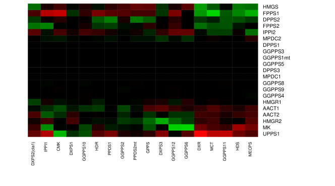
Figure 4: Estimated effects of Mevalonate pathway genes (rows) on the activity of non-mevalonate pathway genes (columns) in A. thaliana. Green/ red indicate positive/ negative values. Genes were ordered using hierarchical clustering.

We apply the LARN algorithm on a microarray dataset containing expressions of several genes in the flowering plant Arabidopsis thaliana (Wille et al, 2004). In this dataset, gene expressions are collected from $n=118$ samples, which are plants grown under different experimental conditions. We take the expressions of $q=18$ genes in the non-mevalonate pathway for biosynthesis of isoprenoid compounds, which are key compounds affecting plant metabolism as our multiple responses, and expressions of $p=21$ genes corresponding to the mevalonate pathway as predictors.

Here we want to find out the extent of crosstalk between genes in the two pathways. We apply LARN, and the three methods mentioned before, on the data and evaluate them based on predictive accuracy of 1000 random splits with 100 training samples and 18 test samples: using 5-fold cross-validation to choose optimum values of tuning parameters. LARN has the smallest average RMSE among the four methods, although that comes at the cost of higher number of estimated non-zero elements on average (Table 2). We summarize the crosstalk between genes in the two pathways by taking elementwise average of the estimated coefficient matrices corresponding to the 1000 random splits. For this average coefficient matrix, we summarize the 10 largest coefficients (in absolute values) in Table 1, and visualize all coefficients in the table through a heatmap in Figure 4.

Method	LARN	TGL	SGL	SepLasso
RMSE (x$10^{-2}$)	4.64 (2.1)	4.74 (2.0)	4.71 (2.1)	4.70 (2.1)
Proportion of non-zero coefficients	0.61 (.008)	0.66 (.014)	0.46 (.008)	0.44 (.019)

Table 1: Performance of all methods in A. thaliana data: mean and standard deviation (in brackets) over 1000 random splits

Coefficient	Mevalonate	Non-Mevalonate
	pathway gene	pathway gene
-0.81	UPPS1	DXR
0.68	MK	GGPPS6
0.67	FPPS1	MCT
0.65	MK	GGPPS12
-0.62	FPPS1	CMK
-0.60	UPPS1	GGPPS11
-0.59	UPPS1	MCT
0.58	UPPS1	CMK
-0.57	FPPS1	IPPI1
-0.56	UPPS1	IPPI1

Table 2: Top 10 between-pathway connections in A. thaliana data found by LARN

Only 3 genes in the Mevalonate pathway: UPPS1, FPPS1 and MK, control the largest interactions. Among the connections in Table 2, UPPS1–DXR, MK–GGPPS6, FPPS1–MCT, MK–GGPPS12 and UPPS1–CMK were found previously by Wille et al (2004) (see figures 2 and 3 therein), while the other five are novel. Our other findings also corroborate those obtained by previous studies: for example, the mevalonate pathway genes GGPPS1,3,5,8,9 do not have much effect on the activity of genes in the other pathway (Wille et al, 2004; Lozano and Świrszcz, 2012).

7 Conclusion

Although several nonconvex penalties exist in the literature, the strength of our penalization scheme lies in the significant scope of inference procedures that can rise from the choice of the reference distribution $F$. Our method shares the weakness of all nonconvex penalties: small signals may go undetected or can be estimated in a biased fashion. However the flexibility in choosing $F$ provides enough motivation for further research in fine tuning similar penalization schemes.

Appendix A Proofs

Proof of Theorem 3.1.

We shall prove a small lemma before going into the actual proof.

Lemma A.1.

For matrices $K\in\mathbb{R}^{l\times k},L\in\mathbb{R}^{l\times m},M\in\mathbb{R}^{m\times k}$,

$$\operatorname*{Tr}(K^{T}LM)={\operatorname*{vec}}^{T}(K)(I_{k}\otimes L)\operatorname*{vec}(M)$$

Proof of Lemma A.1.

From the property of Kronecker products, $(I_{k}\otimes L)\operatorname*{vec}(M)=\operatorname*{vec}(LM)$. The lemma follows since $\operatorname*{Tr}(K^{T}LM)=\operatorname*{vec}^{T}(K)\operatorname*{vec}(LM)$. ∎

Now, suppose $B=B_{0}+U/\sqrt{n}$, for some $U\in\mathbb{R}^{p\times q}$, so that our objective function takes the form

$$T_{n}(U) = \operatorname*{Tr}\left[\left(Y-XB_{0}-\frac{1}{\sqrt{n}}XU\right)^{T}\left(Y-XB_{0}-\frac{1}{\sqrt{n}}XU\right)\right]$$

$$+\lambda_{n}\sum_{j=1}^{p}p^{\prime}_{F}(r_{j}^{*})\left\|b_{0j}+\frac{u_{j}}{\sqrt{n}}\right\|_{2}$$

$$\Rightarrow T_{n}(U)-T_{n}({0}_{p\times q}) = \operatorname*{Tr}\left[\frac{1}{n}U^{T}X^{T}XU-\frac{2}{\sqrt{n}}E^{T}XU\right]$$ (A.1)

$$+\frac{\lambda_{n}}{\sqrt{n}}\sum_{j=1}^{p}p^{\prime}_{F}(r_{j}^{*})\left(\|\sqrt{n}b_{0j}+u_{j}\|_{2}-\|\sqrt{n}b_{0j}\|_{2}\right)$$

$$= \operatorname*{Tr}(V_{1}+V_{2})+V_{3}$$

Since $X^{T}X/n\rightarrow C$ by assumption, we have $\operatorname*{Tr}(V_{1})\rightarrow\operatorname*{vec}^{T}(U)(I_{q}\otimes C)\operatorname*{vec}(U)$ using Lemma A.1. Using the lemma we also get

$$\operatorname*{Tr}(V_{2})=\frac{2}{\sqrt{n}}{\operatorname*{vec}}^{T}(E)(I_{q}\otimes X)\operatorname*{vec}(U)$$

Now $\operatorname*{vec}(E)\sim\mathcal{N}_{nq}({0}_{nq},\Sigma\otimes I_{q})$, so that $(I_{q}\otimes X^{T})\operatorname*{vec}(E)/\sqrt{n}\leadsto W\equiv\mathcal{N}_{pq}({0}_{pq},\Sigma\otimes C)$ using properties of Kronecker products and Slutsky’s theorem.

Let us look at $V_{3}$ now. Denote by $V_{3j}$ the $j$-th summand of $V_{3}$. Now there are two scenarios. Firstly, when $b_{0j}\neq{0}_{q}$, we have $p^{\prime}_{F}(r_{j}^{*})\stackrel{{\scriptstyle P}}{{\rightarrow}}p^{\prime}_{F}(r_{0j})$. Since $\lambda_{n}/\sqrt{n}\rightarrow 0$, this implies $V_{3j}\stackrel{{\scriptstyle P}}{{\rightarrow}}0$ for any fixed $u_{j}$. Secondly, when $b_{0j}={0}_{q}$, we have

$$V_{3j}=\lambda_{n}n^{(s-1)/2}.(\sqrt{n}r^{*}_{j})^{-s}.\frac{p^{\prime}_{F}(r_{j}^{*})\|u_{j}\|_{2}}{(r^{*}_{j})^{-s}}$$

We now have $b^{*}_{j}=O_{p}(1/\sqrt{n})$, and also each term of the gradient vector is $O((r^{*}_{j})^{-s})$ by assumption. Thus $V_{3j}=O_{P}(\lambda_{n}n^{(s-1)/2}\|u_{j}\|_{2})$. By assumption, $\lambda_{n}n^{(s-1)/2}\rightarrow\infty$ as $n\rightarrow\infty$, so $V_{3j}\stackrel{{\scriptstyle P}}{{\rightarrow}}\infty$ unless $u_{j}=0$, in which case $V_{3j}=0$.

Accumulating all the terms and putting them into A we see that

$$T_{n}(U)-T_{n}({0}_{p\times q})\leadsto\begin{cases}\operatorname*{vec}^{T}(U_{1})[(I_{q}\otimes C_{11})\operatorname*{vec}(U_{1})-2W_{1}]&\text{if }U_{0}={0}_{(p-p_{1})q}\\ \infty&\text{otherwise}\end{cases}$$ (A.2)

where rows of $U$ are partitioned into $U_{1}$ and $U_{0}$ according to the zero and non-zero rows of $B_{0}$, respectively, and the random variable $W$ is partitioned into $W_{1}$ and $W_{0}$ according to zero and non-zero elements of $\operatorname*{vec}(B_{0})$. Applying epiconvergence results of Geyer (1994) and Knight and Fu (2000) we now have

$$\operatorname*{vec}(\hat{U}_{1}) \leadsto (I_{q}\otimes C_{11}^{-1})W_{1}$$ (A.3)

$$\operatorname*{vec}(\hat{U}_{0}) \leadsto {0}_{(p-p_{1})q}$$ (A.4)

where $\hat{U}=(\hat{U}_{1}^{T},\hat{U}_{0}^{T})^{T}:=\operatorname*{arg\,min}_{U}T_{n}(U)$.

The second part of the theorem, i.e. asymptotic normality of $\sqrt{n}(\operatorname*{vec}(\hat{B}_{11})-\operatorname*{vec}(B_{01}))=\hat{U}_{1}$ follows directly from (A.3). It is now sufficient to show that $P(\hat{b}_{j}^{(1)}\neq{0}_{q}|b_{0j}={0}_{q})\rightarrow 0$ to prove the oracle consistency part. For this notice that KKT conditions of the optimization problem for the one-step estimate indicate

$$2x_{j}^{T}(Y-X\hat{B}^{(1)})=-\lambda_{n}p^{\prime}_{F}(r_{j}^{*})\frac{b_{j}^{(1)}}{r_{j}^{(1)}}\quad\Rightarrow\quad\frac{2x_{j}^{T}(Y-X\hat{B}^{(1)})}{\sqrt{n}}=-\frac{\lambda_{n}p^{\prime}_{F}(r_{j}^{*})}{\sqrt{n}}.\frac{b_{j}^{(1)}}{r_{j}^{(1)}}$$ (A.5)

for any $1\leq j\leq p$ such that $\hat{b}_{j}^{(1)}\neq{0}_{q}$. Since $p^{\prime}_{F}(r_{j}^{*})=D^{-}((r_{j}^{*})^{-s})=O_{P}(\|(b_{0j}+1/\sqrt{n}\|^{-s})$ and $\lambda_{n}n^{(s-1)/2}\rightarrow\infty$, the right hand side goes to $-\infty$ in probability if $b_{0j}={0}_{q}$. As for the left-hand side, it can be written as

$$\frac{2x_{j}^{T}(Y-X\hat{B}^{(1)})}{\sqrt{n}}=\frac{2x_{j}^{T}X.\sqrt{n}(B_{0}-\hat{B}^{(1)})}{n}+\frac{2x_{j}^{T}E}{\sqrt{n}}=\frac{2x_{j}^{T}X\hat{U}_{n}}{n}+\frac{2x_{j}^{T}E}{\sqrt{n}}$$

Our previous derivations show that vectorized versions of $\hat{U}_{n}$ and $E$ have asymptotic and exact multivariate normal distributions, respectively. Hence

$${\mathbb{P}}\left[\hat{b}_{j}^{(1)}\neq{0}_{q}|b_{0j}={0}_{q}\right]\leq P\left[2x_{j}^{T}(Y-X\hat{B}^{(1)})=-\lambda_{n}p^{\prime}_{F}(r_{j}^{*})\frac{b_{j}^{(1)}}{r_{j}^{(1)}}\right]\rightarrow 0$$

∎

Proof of Lemma 3.2.

See the proof of corollary 2 of Obozinski et al. (2011) in Appendix A therein. Our proof follows the same steps, only replacing $\Sigma_{SS}$ with $\Sigma\otimes C_{11}$.

∎

Proof of Theorem 4.1.

We broadly proceed in a similar fashion as the proof of Theorem 3 in Zou (2006). As a first step, we decompose the mean squared error:

$$E[\hat{\theta}(F,\lambda)-\theta]^{2} = E[\hat{\theta}(F,\lambda)-z]^{2}+E(z-\theta)^{2}+2E[\hat{\theta}(F,\lambda)(z-\theta)]-2E[z(z-\theta)]$$

$$= E[\hat{\theta}(F,\lambda)-z]^{2}+E\left[\frac{d\hat{\theta}(F,\lambda)}{dz}\right]-1$$

by applying Stein’s lemma (Stein, 1981). We now use Theorem 1 of Antoniadis and Fan (2001) to approximate $\hat{\theta}(F,\lambda)$ in terms of $y$ only. By part 2 of the theorem,

$$\hat{\theta}(F,\lambda)=\begin{cases}0\quad&\text{if }|z|\leq\lambda p_{0}(F)\\ z-\text{sign}(z).\lambda D^{-}_{1}(\hat{\theta}(F,\lambda),F)&\text{if }|z|>\lambda p_{0}(F)\end{cases}$$ (A.6)

Moreover, applying part 5 of the theorem,

$$\hat{\theta}(F,\lambda)=z-\text{sign}(z).\lambda D^{-}_{1}(z,F)+o(D^{-}_{1}(z,F))$$ (A.7)

for $|z|>\lambda p_{0}(F)$. Thus we get

$$[\hat{\theta}(F,\lambda)-z]^{2}=\begin{cases}z^{2}&\text{if }|z|\leq\lambda p_{0}(F)\\ \lambda^{2}D^{-}_{1}(z,F)^{2}+k_{1}(|z|)&\text{if }|z|>\lambda p_{0}(F)\end{cases}$$ (A.8)

and

$$\frac{d\hat{\theta}(F,\lambda)}{dz}=\begin{cases}0&\text{if }|z|\leq\lambda p_{0}(F)\\ 1+\lambda D^{-}_{2}(z,F)+k_{1}^{\prime}(|z|)&\text{if }|z|>\lambda p_{0}(F)\end{cases}$$ (A.9)

where $k_{1}(|z|)=o(|z|)$, and $D^{-}_{2}(z,F)=d^{2}D^{-}(z,F)/dz^{2}$. Thus

$$E[\hat{\theta}(F,\lambda)-\theta]^{2} = E[z^{2}{\mathbb{I}}_{|z|\leq\lambda p_{0}(F)}]+E\left[\left(\lambda^{2}D^{-}_{1}(|z|,F)^{2}+2\lambda D^{-}_{2}(|z|,F)+2+\right.\right.$$ (A.10)

$$\left.\left.k_{1}(|z|)+k_{1}^{\prime}(|z|)\right){\mathbb{I}}_{|z|>\lambda p_{0}(F)}\right]-1$$

Now

$$k_{1}(|z|) = \lambda^{2}\left[D^{-}_{1}(z,F)^{2}-D^{-}_{1}(\hat{\theta}(F,\lambda),F)^{2}\right]\quad\leq\quad\lambda^{2}c_{1}^{2},\text{ and}$$

$$|k_{1}^{\prime}(|z|)| = \lambda\left|D^{-}_{2}(z,F)-\frac{dD^{-}_{1}(\hat{\theta}(F,\lambda),F)}{dz}\right|\quad\leq\quad 2\lambda c_{2}$$

Substituting these in (A.10) above we get

$$E[\hat{\theta}(F,\lambda)-\theta]^{2} \leq \lambda^{2}p_{0}(F)^{2}P[|z|\leq\lambda p_{0}(F)]+E\left[\left(\lambda^{2}f^{2}(|z|)+2\lambda D^{-}_{2}(z,F)\right)BI_{|z|>\lambda p_{0}(F)}\right]$$ (A.11)

$$+\lambda^{2}c_{1}^{2}+2\lambda c_{2}+1$$

$$\leq 2\lambda^{2}c_{1}^{2}+4\lambda c_{2}+1$$

$$\leq 4\lambda^{2}c_{1}^{2}+8\lambda c_{2}+1$$

Adding and subtracting $z^{2}{\mathbb{I}}_{|z|>\lambda p_{0}(F)}$ to the first and second summands of (A.10) above, we also have

$$E[\hat{\theta}(F,\lambda)-\theta]^{2} = Ez^{2}+E\left[\left(\lambda^{2}D^{-}_{1}(z,F)^{2}+2\lambda D^{-}_{2}(z,F)+2-y^{2}+\lambda^{2}c_{1}^{2}\right.\right.$$ (A.12)

$$\left.\left.+2\lambda c_{2}\right){\mathbb{I}}_{|z|>\lambda p_{0}(F)}\right]-1$$

$$\leq (2\lambda^{2}c_{1}^{2}+4\lambda c_{2})P[|z|>\lambda p_{0}(F)]+\theta^{2}$$

Following Zou (2006), $P[|z|>\lambda p_{0}(F)]\leq 2q(\lambda p_{0}(F))+2\theta^{2}$, with $q(x)=\exp[-x^{2}/2]/(\sqrt{2\pi}x)$. Thus

$$E[\hat{\theta}(F,\lambda)-\theta]^{2} \leq 2(2\lambda^{2}c_{1}^{2}+4\lambda c_{2})[q(\lambda p_{0}(F))+\theta^{2}]+\theta^{2}$$ (A.13)

$$\leq (4\lambda^{2}c_{1}^{2}+8\lambda c_{2}+1)[q(\lambda p_{0}(F))+\theta^{2}]$$

Combining this with (A.11) we get

$$E[\hat{\theta}(F,\lambda)-\theta]^{2}\leq[4(\lambda c_{1}+1)^{2}-3][q(\lambda p_{0}(F))+\min(\theta^{2},1)]$$ (A.14)

assuming without loss of generality that $c_{1}\geq c_{2}$. Since $R(\text{ideal})=\min(\theta^{2},1)$ and $q(x)\leq(\sqrt{2\pi}x)^{-1}<1/x$, we have the needed. ∎

Appendix B Additional simulations

We present the simulation results corresponding to $\rho=0$, $\rho=.5$ and $\rho=.9$ in Figures 5, 6 and 7, respectively. The results are similar to the case of $\rho=.7$ presented in the main paper. LARN has the lowest MAE in all cases, and the lowest cv-RMSE in all but one (Case (a) for $\rho=0$) cases.

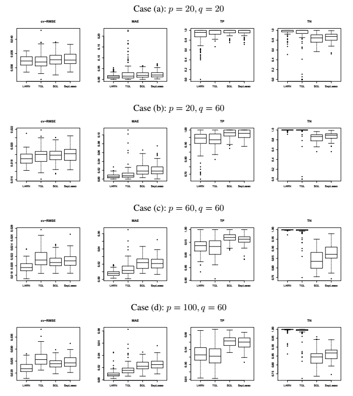
Figure 5: Boxplots of evaluation metrics for all methods in different $(p,q)$ settings: $\rho=0$.

Figure 6: Boxplots of evaluation metrics for all methods in different $(p,q)$ settings: $\rho=0.5$.

Figure 7: Boxplots of evaluation metrics for all methods in different $(p,q)$ settings: $\rho=0.9$.

References

- Antoniadis and Fan (2001) A. Antoniadis and J. Fan. The Adaptive Lasso and Its Oracle Properties. J. Amer. Statist. Assoc., 96:939–967, 2001.
- Buhlmann and van de Geer (2011) P. Buhlmann and S. van de Geer. Statistics for High-Dimensional Data. Methods, Theory and Applications. Springer, 2011.
- Chen et al. (2014) W.-P. Chen, Y. N. Wu, and R.-B. Chen. Bayesian Variable Selection for Multi-response Linear Regression, pages 74–88. Springer International Publishing, Cham, 2014. ISBN 978-3-319-13987-6. doi: 10.1007/978-3-319-13987-6˙8. URL http://dx.doi.org/10.1007/978-3-319-13987-6_8.
- Chen et al. (2012) X. Chen, J. He, R. Lawrence, and J. G. Carbonell. Adaptive Multi-task Sparse Learning with an Application to fMRI Study. In Proceedings of the 2012 SIAM International Conference on Data Mining, volume 12, 2012. DOI: http://dx.doi.org/10.1137/1.9781611972825.19.
- Donoho and Johnstone (1994) D. Donoho and I. Johnstone. Ideal Spatial Adaptation via Wavelet Shrinkages. Biometrika, 81:425–455, 1994.
- Fan and Chen (1999) J. Fan and J. Chen. One-Step Local Quasi-Likelihood Estimation. J. R. Statist. Soc. B, 61:927–943, 1999.
- Fan and Li (2001) J. Fan and R. Li. Variable Selection via Nonconcave Penalized Likelihood and its Oracle Properties. J. Amer. Statist. Assoc., 96:1348–1360, 2001.
- Geyer (1994) C. Geyer. On the Asymptotics of Constrained M-Estimation. Ann. Statist., 22:1993–2010, 1994.
- Jornsten (2004) R. Jornsten. Clustering and classification based on the depth. J. Multivariate Anal., 90:67–89, 2004.
- Knight and Fu (2000) K. Knight and W. Fu. Asymptotics for Lasso-Type Estimators. Ann. Statist., 28:1356–1378, 2000.
- Li et al. (2015) Y. Li, B. Nan, and J. Zhu. Multivariate Sparse Group Lasso for the Multivariate Multiple Linear Regression with an Arbitrary Group Structure. Biometrics, 71:354–363, 2015.
- Liu (1990) R.Y. Liu. On a notion of data depth based on random simplices. Ann. Statist., 18:405–414, 1990.
- Loh and Wainwright (2015) P.-L. Loh and M. J. Wainwright. Regularized -estimators with Nonconvexity: Statistical and Algorithmic Theory for Local Optima. J. Mach. Learn. Res., 16:559–616, 2015.
- Lozano and Świrszcz (2012) A. Lozano and G. Świrszcz. Multi-level lasso for sparse multi-task regression. In John Langford and Joelle Pineau, editors, Proceedings of the 29th International Conference on Machine Learning (ICML-12), pages 361–368, New York, NY, USA, 2012. ACM. URL http://icml.cc/2012/papers/207.pdf.
- Molstad and Rothman (2016) A. J. Molstad and A. J. Rothman. Indirect multivariate response linear regression. Biometrika, 103:595–607, 2016.
- Mosler (2013) K. Mosler. Depth statistics. In C. Becker, R. Fried, and S. Kuhnt, editors, Robustness and Complex Data Structures, pages 17–34. Springer Berlin Heidelberg, 2013. ISBN 978-3-642-35493-9. doi: 10.1007/978-3-642-35494-6˙2.
- Narisetty and Nair (2016) N. N. Narisetty and V. N. Nair. Extremal Depth for Functional Data and Applications. J. Amer. Statist. Assoc., 111:1705–1714, 2016.
- Neghaban and Wainwright (2011) S. Neghaban and M. J. Wainwright. Simultaneous support recovery in high dimensions: Benefits and perils of block -regularization. IEEE Trans. Inf. Theory, 57:3841–3863, 2011. doi: 10.1017/S1461145713001296.
- Neghaban et al. (2009) S. N. Neghaban, B. Yu, M. J. Wainwright, and P. Ravikumar. A unified framework for high-dimensional analysis of -estimators with decomposable regularizers. In Advances in Neural Information Processing Systems, pages 1348–1356, 2009.
- Obozinski et al. (2011) G. Obozinski, M. J. Wainwright, and M. I. Jordan. Support Union Recovery in High-dimensional Multivariate Regression. Ann. Statist., 39:1–47, 2011.
- Peng et al. (2016) B. Peng, L. Wang, and Y. Wu. An Error Bound for -norm Support Vector Machine Coefficients in Ultra-high Dimension. J. Mach. Learn. Res., 17:1–26, 2016.
- Rothman et al. (2010) A. J. Rothman, E. Levina, and J. Zhu. Sparse Multivariate Regression With Covariance Estimation. J. Comp. Graph. Stat., 19:947–962, 2010.
- Stein (1981) C. Stein. Estimation of the Mean of a Multivariate Normal Distribution. Ann. Statist., 9:1135–1151, 1981.
- Tibshirani (1996) R. Tibshirani. Regression shrinkage and selection via the lasso. J. R. Statist. Soc. B, 58(267–288), 1996.
- Tukey (1975) J.W. Tukey. Mathematics and picturing data. In R.D. James, editor, Proceedings of the International Congress on Mathematics, volume 2, pages 523–531, 1975.
- Vincent and Hansen (2014) M. Vincent and N. R. Hansen. Sparse group lasso and high dimensional multinomial classification. Comput. Statist. Data Anal., 71:771–786, 2014.
- Wang et al. (2013) L. Wang, Y. Kim, and R. Li. Calibrating Nonconvex Penalized Regression in Ultra-high Dimension. Ann. Statist., 41:2505–2536, 2013.
- Wille et al (2004) A. Wille et al. Sparse graphical Gaussian modeling of the isoprenoid gene network in Arabidopsis thaliana. Genome Biol., 5:R92, 2004.
- Yang and Zou (2015) Y. Yang and H. Zou. A fast unified algorithm for solving group-lasso penalize learning problems. Statist. and Comput., 25:1129–1141, 2015.
- Zhang (2010) C. H. Zhang. Nearly Unbiased Variable Selection under Minimax Concave Penalty. Ann. Statist., 38:894–942, 2010.
- Zou (2006) H. Zou. The Adaptive Lasso and Its Oracle Properties. J. Amer. Statist. Assoc., 101:1418–1429, 2006.
- Zou and Li (2008) H. Zou and R. Li. One-step sparse estimates in nonconcave penalized likelihood models. Ann. Statist., 36:1509–1533, 2008.
- Zuo (2003) Y. Zuo. Projection-based depth functions and associated medians. Ann. Statist., 31:1460–1490, 2003.
- Zuo and Cui (2005) Y. Zuo and M. Cui. Depth weighted scatter estimators. Ann. Statist., 33:381–413, 2005.
- Zuo and Serfling (2000) Y. Zuo and R. Serfling. General notions of statistical depth functions. Ann. Statist., 28:461–482, 2000.
- Zuo et al. (2004) Y. Zuo, M. Cui, and X. He. On the Staehl-Donoho estimator and depth-weighted means of multivariate data. Ann. Statist., 32:167–188, 2004.
Supplementary Material for