Abstract

Despite the impressive advances in biological imaging, no imaging modality today generates, in a comprehensive manner, high-resolution images of crowded molecules working deep inside the living cell in real time. In this paper, instead of tackling this engineering problem in the hope of solving it, we ask a converse question: What if such imaging is fundamentally impossible? We argue that certain decoherence processes could be suppressed because the internal workings of the cell are not being closely “observed” in the quantum mechanical sense, as implied by the assumed impossibility of imaging. It is certainly true that the “wet and warm” living cell should not exhibit quantum behavior merely because of the lack of observation. Despite this, we plow ahead to see what might result from such absence of the outward flow of information. We suggest that chaotic dynamics in the cell could be quantum mechanically suppressed — a known phenomenon in quantum chaology, which is potentially resistant to various mechanisms for the emergence of classicality. We also consider places where experimental evidence for/against such a possibility may be sought.

1 Introduction

The central premise, or at least the central working hypothesis, of modern biology states that all forms of life, including us, are molecular machines. One might actually go further to assert that every form of life is essentially a classical molecular machine. A few qualifications are needed for this stronger version. First, without quantum physics we do not even have the stability of atoms and molecules, or their chemical reactions, not to mention the non-infinite specific heat of the vacuum. However, we may still be able to construct a classical model that describes interactions of molecules so that it successfully captures essential dynamics of the biological machine; much like the way workings of a transistor can reasonably be modeled with a few characteristic curves and/or equivalent circuits, hiding the “quantum-mechanical layer” — an abstraction layer in the computer engineering sense — of silicon atoms and electron waves underneath. Second, several emerging aspects of life being investigated under the heading of “quantum biology” challenge the view that life is basically classical. These aspects include photosynthesis [1, 2] and magnetic sensing by European robins [3]. Although these phenomena are intriguing, it is fair to say that these are either a relatively short-time phenomenon where the associated energy quanta $\hbar\omega$ far exceed the thermal energy $k_{B}T$ as in the former, or a small-scale phenomenon occurring in — presumably, because the detail is not yet known — space spanning at most a few molecules, as in the latter. In other words, in retrospect, these quantum phenomena are found where they are expected, i.e. when the length or time scale is small, or only modestly larger than the scale where quantumness certainly is expected.

In this paper, we propose a new perspective to study the relevance of quantum mechanics in biology, possibly extending the arena where quantum physics plays a role. The main idea is the following. It is extremely difficult to devise an experimental method that enables comprehensive, molecular-resolution, real-time, volume-imaging (CMRV) of the living cell. The word “comprehensive” is added to mean that most molecules, as opposed to e.g. fluorescently labeled molecules that are a small fraction of the whole, can be observed simultaneously. True three dimensional (3D) imaging is meant by the word “volume imaging”, that has the ability to see internal structures and therefore goes beyond quasi-3D methods such as 3D topography enabled by the atomic force microscope (AFM). The stated extreme difficulty to devise a CMRV method is justified because otherwise somebody capable would have invented it, considering the utility such a CMRV method would offer to biology research. Turning this circumstance on its head, if the difficulty is not of practical but of fundamental character, then little information about the internal states of the cell is leaking to the outside environment because otherwise we would be able to measure it in principle. If this reasoning is correct, then the system is somewhat isolated, that in turn means quantum mechanically more coherent evolution is expected to a certain degree, which we later attempt to estimate.

The idea, that there is some connection between a biological object and quantum measurement on it, is by no means new: Already in 1932 Bohr discussed the connection noting that, in effect, a biological object might “hide its ultimate secrets” because a high-resolution measurement would destroy the object [4]. Fast-forwarding to modern times, Henderson noted that all high-resolution imaging methods in biology, be it X-ray diffraction or electron microscopy, are limited by radiation damage to the biological specimen [5]. It is true that a variety of methods — X-ray crystallography, cryoelectron microscopy, nuclear magnetic resonance (NMR) spectroscopy, scanning probe microscopy and “super-resolution” optical microscopy to name a few — have had remarkable successes in supporting biology research. However, these are complementary and each of these has a limited domain of applicability, for otherwise we would have a different or shorter list of methods in the above. Furthermore, as we will elaborate on later, each method has its own fundamental limits and whether CMRV will ever be possible is an open question. In the present work, while some attempts are made to justify the fundamental impossibility of CMRV, we will eventually assume such impossibility in order to see whether something interesting follows from the assumption. Meanwhile, those who assume the opposite should be encouraged to develop a CMRV method.

The idea, that quantum mechanics plays a significant role in biology at a larger scale than what are already mentioned, has also long history. Several authors that include prominent figures proposed since no later than 1967 that the human brain might be quantum mechanically coherent, although this certainly is far from the mainstream view [6, 7, 8]. While the brain is outside the scope of the present work, a work that critically investigates the connection between the brain and quantum physics is relevant [9]. Briefly, this work concludes that the brain is such a dissipative system that dissipation-induced decoherence takes place far too quickly for any quantum coherence to survive. The question of whether the whole biological cell, as opposed to the whole brain, is quantum mechanically coherent has also been asked [10]. Their work, which also is far from the mainstream view, nonetheless contains at least one reasonable point that the internal workings of the cell are “observed” by the environment with possibly unconventional pointer states [11], to which the wavefunction “collapses”. Much as these studies are inspiring, it is perhaps fair to say that these are controversial at best, mainly because it is so unlikely to have quantum coherence in such “wet and warm” physical systems. To see this, it is sufficient to consider the amount of effort it takes to build any quantum-enhanced instrument: That involves e.g. cooling, calibrating, vibration-damping, removing external noise, characterising intrinsic noise, and so on so forth. Nonetheless, we do not have a proof that quantum effects — of the sort we are discussing — do not appear in wet-and-warm systems, because we do not fully understand the nature of the quantum-classical boundary.

The emergence of classicality is explained in several ways. First, classical mechanics is in a sense the short-wavelength limit of quantum mechanics and as such it emerges exactly the same way as ray optics emerges from wave optics. In this view, classicality emerges whenever the potential is smooth in the scale of the de Broglie wavelength. Second, things become classical when the action $S$ involved is much larger than $2\pi\hbar$. Loosely speaking, when a characteristic time scale of the system is $\tau$, with the associated characteristic frequency scale $\omega\sim 2\pi/\tau$, then classicality requires $E\gg\hbar\omega$, where $E\sim S/\tau$ is a characteristic energy. Quantization manifests itself when the particle energy such as $\hbar\omega$, which tends to be larger for lighter particles, is larger than a characteristic energy scale of the system. Such characteristic energy scale may be the thermal energy $k_{B}T$ in a system embedded in an environment. This explains why most quantum experiments demand cryogenic temperatures, besides ones involving optical photons for example. However, these conditions are still not complete: Microscopic quantum uncertainty could always be amplified to a macroscopic quantum uncertainty since quantum mechanics is linear, as exemplified by Schrodinger’s cat. The third way, in which classicality emerges, is decoherence due to interaction with the environment [12]. In this view, we as part of the environment get totally entangled with Schrodinger’s cat so that we do not notice the superposition. The importance of isolation of the system from the environment is emphasized here. For example, setting aside the subtlety due to the highly mixed nature of the states, NMR quantum computing works because of isolation, in spite of the condition $k_{B}T\gg\hbar\omega$. One way the amplification of minute quantum uncertainty happens drastically is when the system’s classical dynamics is chaotic; because the trajectory depends on the initial condition in an exponentially sensitive way. For example, amplification of quantum uncertainty to the macroscopic level in a surprisingly short time has been discussed with respect to very macroscopic objects including the Saturn’s satellite Hyperion [13]. It is only the interaction with the environment, partly in the form of impinging photons in this case, that keeps Hyperion classical. In the present work, we look into the possibility that the biological cell is classically chaotic and is not that well-observed by the environment as Hyperion is. Specifically, we consider possible delocalization of biological molecules in the cell, however provocative this possibility may seem.

This paper is organized as follows. A variety of biological imaging methods, established ones and also proposed ones, are discussed in Sec. 2 to show that the unattainability of CMRV is a serious possibility. In Sec. 3 we first estimate how much “information” leaks out to the environment from the living cell. We then consider how these findings fit with what we know in quantum chaology including, in particular, quantum suppression of classical chaos. We consider potential observational or experimental consequences in case such quantum suppression of chaos is indeed at work. Section 4 concludes the paper. Throughout the paper we will use the SI system of units. Symbols $c$, $\varepsilon_{0}$, $\hbar$ and $k_{B}$ respectively represent the speed of light, the vacuum permittivity, the reduced Planck’s constant and the Boltzmann constant, of which some have appeared already. Some symbols such as $\lambda$ stand for multiple things (e.g. wavelength and Lyapunov exponent) in this paper to avoid cluttered presentation. The meanings of such symbols should be clear from the context.

2 Biological imaging methods and their limits

In this section, we intend to show that unattainability of CMRV of the cell is a serious possibility. Beautiful results from biology research can be at the same time misleading because they may give an impression that any biological measurement is possible. However, on a closer look one finds that each reported measurement was preceded by setting up particularly favorable conditions generally incompatible with other measurement methods, and furthermore each measurement method is associated with various fundamental limits. Hence it is entirely possible that CMRV is impossible.

We examine several biological measurement methods in the following. A particular emphasis is on methods under development. While we also try to present a broad perspective, we do not intend to give a full review of established methods that are already widely used.

2.1 X-ray

X-ray methodologies used in biology are diverse. Some use soft X-rays, especially in the so-called “water window” at the wavelength of $2.34\mathrm{nm}\sim 4.4\mathrm{nm}$, and others use hard X-rays. Some use optical elements such as lens and mirror, while others including crystal diffraction are lensless. While there have been much progress on all these fronts [14], it remains true that the X-ray damages biological specimen generally more than electrons do for a given amount of structural information retrieved, mainly by photo-ionization [5]. X-ray photons simply are so energetic. Hence the specimen is destroyed before a sufficient number of X-ray photons are collected to form an image. Whereas atomic-resolution structures of biological molecules are routinely obtained in X-ray crystallography because a large number of copies of the same molecules are involved, when it comes to single, unique objects such as a structure in a cell, X-ray methods are generally no better than the electron-based counterpart in terms of radiation damage [5].

The advent of the method called flash X-ray imaging [15, 16] makes an interesting twist to the above picture. The X-ray free electron laser (XFEL) invented long ago [17] has come to fruition after many years of effort and is capable of producing intense and short ($\sim\mathrm{fs}$) X-ray pulses. The idea is that the inertia of atomic mass is no longer negligible at the femto-second time scale and hence the atomic nuclei stay where they are during the X-ray irradiation; despite the ionization of atoms due to the intense X-ray. Thus, a diffraction image can be recorded “before” the specimen is destroyed. Perhaps surprisingly to the uninitiated, phase information is generally in the diffraction pattern to allow for reconstruction [18, 19]. Nevertheless, $10^{5}\sim 10^{6}$ identical copies of the molecule (or molecular complex) are still needed to get a 3D “near-atomic resolution” structure with currently foreseeable technology because each image is essentially 2D [20]. However, 3D imaging using a single copy of the specimen must be possible to begin to realize CMRV. (Those who think that CMRV is obviously impossible because the X-ray destroys the specimen, will find an argument based on reconstruction of the specimen below.) One way might be the use of tomography with multiple and almost simultaneous X-ray pulses from different angles. Another possible way is the use of “ankylography”, whose feasibility is under active research [21].

Assuming that 3D image acquisition is possible in flash X-ray imaging, we examine whether this imaging method would make CMRV possible. First, we get one glaring point out of the way: X-ray flash imaging seems to be fundamentally destructive for real-time imaging because the specimen would be evaporated after filming only a single frame of the movie. However, there is a rather strange possibility: We could, in principle, reconstruct the specimen each time, based on the recorded full structural information, possibly using a molecular-precision synthetic biology method [22]. Despite the progress in synthetic biology, however, no method today is capable of building things out of molecular parts in a well-controlled way. However, if we assume the realizability of such a method, one could in principle produce a movie of a biological process with a time step $\Delta t$ as follows: We first bring a frozen specimen to room temperature for the period $\Delta t$, which is followed by rapid vitrification of the specimen by cooling it down to a cryogenic temperature again (see discussions on cryoelectron microscopy below). X-ray flash imaging is then performed to generate structural data of the specimen. The data in turn is used to reconstruct, by a cryogenic process, the next specimen to repeat the process. Evidently, this is speculative at best and the minimum possible interval $\Delta t$ perhaps is not short enough for some important scientific questions. Since this notion will appear repeatedly in this paper, we call this method reconstruction-based cryogenic stop-motion photography (RCSP).

Second, the larger the number of voxels is, the more intense the needed X-ray pulse is, in order to have a sufficient number of photons to acquire enough information. However, the oscillating electric field of the X-ray field cannot be arbitrarily large for the following reason. To observe atomic details with diffraction, we need X-ray with the wavelength of about the Bohr radius $a_{0}=4\pi\varepsilon_{0}\hbar^{2}/m_{e}e^{2}$, where $m_{e}$ is the electron mass. According to the standard approximation, an electron bound to an atomic nucleus is regarded free because the X-ray frequency is much larger than the “orbital frequency” of the bound electron. Hence classically we have

$$m_{e}\ddot{x}=eE\cos\left(\omega t\right),$$ (1)

where $\omega=2\pi c/\lambda=2\pi c/a_{0}=cm_{e}e^{2}/2\varepsilon_{0}\hbar^{2}$ is the angular frequency of the X-ray and $E$ is the associated electric field amplitude. Plugging $x=-x_{0}\cos\left(\omega t\right)$ in Eq.(1), we obtain $x_{0}=eE/m_{e}\omega^{2}$, which is the motional amplitude of the electron being “shaken” by the X-ray field. A problem begins to emerge when the X-ray field is so strong that $x_{0}$ approaches the Bohr radius $a_{0}$, because then the electron approaches the neighboring atoms. Up to a numerical constant of the order of $1$, the electric field at which $x_{0}\sim a_{0}$ is $E_{\mathrm{shake}}=m_{e}^{2}c^{2}e/4\pi\varepsilon_{0}\hbar^{2}\cong 10^{16}\mathrm{V/m}$. The flow of energy $J$ due to such an X-ray pulse is

$$J=\varepsilon_{0}E_{\mathrm{shake}}^{2}c\sim 10^{29}\mathrm{W/m^{2}}.$$ (2)

On the other hand, Fig. 2 of Ref.[20] shows that the Linac Coherent Light Source (LCLS) has the X-ray brilliance of $\sim 10^{24}\mathrm{(photon/s/0.1\%bw/mm^{2}/mrad^{2})}$. A decent diffraction experiment should require $0.01\%$ bandwidth monochromaticity and $0.1\mathrm{mrad}$ beam divergence because both the monochromaticity and the beam divergence need to be roughly the wavelength divided by the specimen size, where the specimen size is $\sim 1\mu\mathrm{m}$ in our case of single biological cells. Note that the coherence requirements become increasingly demanding for larger specimens. Hence we have $J\sim 10^{18}\mathrm{W/m^{2}}$ since each X-ray photon has energy of $\sim 12\mathrm{keV}\sim 10^{-15}\mathrm{J}$. On the other hand, Ref.[20] states towards the end that one needs $10^{5}\sim 10^{6}$ specimens and $100$-fold increase of the X-ray peak power to enable atomic resolution 3D imaging. Taking this at the face value, this would mean up to 8 orders of magnitude increase of the X-ray power might be needed if we want to obtain an one-shot diffraction image with a single specimen, resulting in a figure $J\sim 10^{26}\mathrm{W/m^{2}}$. Comparing with Eq.(2), we have leeway of only a few orders of magnitude. This crude calculation suggests that at least more careful evaluation is desired for the flash X-ray method if it aspires to enable CMRV. Even assuming this is not a problem, the electron-positron pair production begins at the Schwinger limit $E_{S}=E_{\mathrm{shake}}/\alpha$, where $\alpha\cong\left(137\right)^{-1}$ is the fine structure constant [23]. This suggests a possibly general trend that higher power brings in new physics that has to be dealt with.

2.2 Electron microscopy

Despite the impressive progress in biological electron microscopy (EM), the resolution-limiting factor of biological EM remains to be radiation damage to the specimen by the probe electrons. Hence the situation is qualitatively similar to the case of X-ray. However, flash imaging with electrons seems somewhat contrived at least at the fundamental level since the electrons are fermions and moreover they electrostatically repel each other. In this subsection, in spite of the growing relevance of e.g. serial block-face scanning EM (SEM) in the brain “connectmics” research [24], we focus on transmission EM (TEM) that is relevant in molecular and/or atomic scale imaging.

The art of biological TEM is multifaceted. The traditional methods use protocols such as plastic embedding and heavy metal staining. The reason for the latter is that the Coulomb force from the atomic nuclei is the main scattering mechanism in TEM. These protocols work excellently and led to many important discoveries at the scale of organelles, but they introduce artefacts at the molecular scale. Thus, cryoelectron microscopy (cryoEM) [25, 26] was introduced in order to enable molecular or atomic scale resolution in biological TEM. CryoEM uses “frozen” specimens at cryogenic temperatures (typically the liquid nitrogen temperature) and hence the specimen can be placed in a vacuum in its “original” form. In order to prevent the growing ice crystals from destroying fine biological structures, the method uses liquid ethane, to which the thin specimen is rapidly dropped. The reason is that liquid ethane tends to have less bubbles than liquid nitrogen does and hence allows for a better thermal contact. Hence the specimen is rapidly vitrified and the water remains in the glassy state. It is widely believed that the specimen prepared as mentioned represents a biologically relevant, natural structure. However, the contrast is very weak in cryoEM because typical biological specimens contain mostly light elements. Moreover, one can use only a limited dose of electrons of at most $\sim 10{}^{3}e/\mathrm{nm}^{2}$ because of radiation damage to the specimen caused by the very electrons used for imaging. Hence, the resolution is limited by shot noise, which is a fundamental consequence of the electron being a particle.

Before proceeding, we comment on TEM in the broader context. TEM has been used also in materials science since the beginning, where the resolution had long been limited by lens aberration. The aberration has finally been corrected in the 90’s [27, 28], fifty years after Scherzer showed possible solutions [29]. Atomic resolution images are now routinely obtained for beam-insensitive inorganic specimens. Furthermore, a study using aberration-corrected TEM presents beautiful pictures of organic molecules in the carbon nanotube [30]. Low-voltage, aberration-corrected electron microscopes have been developed around the globe, enabling imaging of beam-sensitive specimens [31, 32, 33]. However, few things should be kept in mind. First, aromatic molecules or ones with a similar structure, such as the nanotube, are very stable and highly resistant against radiation damage; while most biological molecules are not. Second, the specimen used in Ref.[30] is very thin, whereas molecules of biological interest can be as large as $30\mathrm{nm}$ and the vitrified specimen must be thick accordingly. However, a thicker specimen requires higher beam energy in TEM, which could produce knock-on damage. More importantly, the secondary electrons generated by single inelastic scattering events produce more damage in thick specimens. In short, beautiful pictures of organic molecules in nanotubes do not mean that the same quality of images can be obtained in other situations such as cryoEM of biologically interesting molecules.

At least two ways to bypass the radiation damage problem have been successfully developed and these are established methodologies in structural biology today [34]. Both of these are based on averaging to improve the signal-to-noise (S/N) ratio using multiple copies of the same molecule. The first method is electron crystallography that often use 2D crystals, which are not easy to prepare. The second method is called “single-particle analysis”, where many identical molecules are prepared in vitreous ice without crystallizing them. Although each molecule has a random orientation, approximate orientations of the molecules may be determined from the noisy raw data, thus allowing us to average images of similarly-oriented molecules, resulting in a better S/N of the estimated structure. This in turn allows us to obtain a better estimation of molecular orientations by fitting the estimated structure to the raw data. Iterating this, one can increasingly refine the computed structure; although obviously there are pitfalls associated with this clever method that generates useful data from very noisy raw data. The uninitiated reader should note that intricate structures obtained with cryoEM found in the scientific literature are likely to be the result of such averaging and data processing. In such cases, these structures do not represent the raw resolving power of cryoEM. The resolution of raw data remained to be $5\sim 10\mathrm{nm}$ because of radiation damage at least until recently, when improved electron detectors began to be widely used [35].

Ideas for potential future improvements to cryoEM are in the pipeline. The so-called “interaction-free measurement”, which is capable of detecting an photon-absorbing object without actually getting photons absorbed, was first proposed long ago [36]. Subsequently, it was significantly refined so that the failure probability can be brought down arbitrarily close to zero [37], and finally its use in biological EM was proposed [38]. While interaction-free measurement is inspiring, its use is limited when it comes to distinguishing two semi-transparent objects, as opposed to distinguishing the vacuum and a semi-transparent object [39]. However, this aspect is important because one would like to distinguish, e.g. protein and water in cryoEM. Another proposed way to improve cryoEM is the use of superconducting qubits to achieve measurement at the Heisenberg limit, rather than at the the shot-noise limit [40, 41]. This latter scheme may improve the resolution of cryoEM but it will likely fall short of achieving the atomic resolution. The simple reason, after all, is that imaging methods using electrons are fundamentally destructive. A possible way to get around this difficulty would be the use of RCSP. Again, this possibility is speculative at best.

2.3 NMR

NMR occupies a unique position in biological imaging because it does not belong to the usual category where the incident wave scattered by a specimen is measured. The frequency $\nu$ of the electromagnetic wave is at most on the order of $1\mathrm{GHz}$ and hence the photon energy $h\nu$ is at most $\sim 10\mu\mathrm{eV}$, which is far smaller than energy scales associated with an X-ray or an electron beam, or even $k_{B}T$ at room temperature. Consequently, specimen damage is minimal, if not zero, in NMR and this represents perhaps the most attractive aspect of NMR. The downside of this is the weak signal to be detected, which typically translates to a slow data acquisition rate.

We first broadly review relevant aspects of NMR. As is well known, volume imaging with NMR is routinely done today with clinical magnetic resonance imaging (MRI), where the spatial resolution is typically $\sim 1\mathrm{mm}$. Using dedicated instruments, the MRI resolution has been pushed down to $\sim 1\mu\mathrm{m}$ for small specimens [42]. We also note that NMR has widely been used to determine protein structures, using a solution containing a massive number of the same molecule of interest. A number of techniques are associated with such methods and reviewing NMR spectroscopy in a decent way is firmly beyond the scope of this paper. Hence, in what follows, we focus on methods that seem relevant to CMRV.

One method that aspires to enable CMRV is magnetic resonance force microscopy (MRFM) [43, 44]. The method has been improving ever since its introduction, resulting in a relatively recent demonstration of biological imaging with resolution $<10\mathrm{nm}$ [45]. A conceptually similar yet distinct method utilizing the nitrogen-vacancy (NV) center in diamond has also been introduced recently [46]. This latter technology, NV magnetometry (NVM), has several distinct usages but here we focus on the one relevant to CMRV, which is nano-scale MRI. We consider whether MRFM/NVM represent a possible path to CMRV. Since future prospects of the methods are nicely summarized in Ref.[47] at least in the case of MRFM, here we point out only few potential obstacles. First, MRFM/NVM is a scanning NMR method and hence, combined with the fact that the weak signal requires integration for a long time, it is slow. This makes real-time imaging difficult, unless RCSP is employed. In any event, high-resolution MRFM/NVM measurements are likely to eventually require cryogenic temperatures to reduce thermal noise and to prevent diffusion of biological molecules. Second, MRFM/NVM employs a magnetic field gradient $\partial B/\partial z$ as in the conventional MRI. The magnitude of the gradient $\partial B/\partial z$ determines the spatial resolution $\Delta z$, in such a way that the field difference

$$\Delta B=\frac{\partial B}{\partial z}\Delta z$$ (3)

corresponds to the attainable frequency resolution $\Delta f$ through the gyromagnetic ratio. There are few possibilities that fundamentally limit the frequency resolution $\Delta f$. First, there is the frequency broadening due to dissipation, that lowers the $Q$ value of the oscillator in MRFM, or in the case of NVM that determines the phase coherence time of the NV center. It is hard to know if such dissipation is intrinsic or extrinsic. Second, there is no motional narrowing in solid state NMR, unlike in bulk liquid NMR. Consequently, almost inevitably we have inhomogeneous broadening $\Delta f$ (besides intrinsic broadening due to dissipation) of the resonance peak [48]. This broadening translates to a largely uncontrollable/unknowable frequency shift of individual nuclear spins (typically that of hydrogen) placed in the inhomogeneous environment, in localized measurements such as ones performed in MRFM/NVM. The spatial resolution limit is reached when such a shift $\Delta f$ matches $\Delta B$ in Eq.(3). On the other hand, the magnetic field gradient is typically produced by a tiny, but strong, magnet placed nearby the biological specimen. Naturally, the field gradient $\partial B/\partial z$ decays quickly as the distance from the magnet increases. This in turn means that we lose resolution fairly quickly as the depth from the specimen surface increases. Hence volume imaging is hard with MRFM/NVM. Consequently, even if MRFM/NVM will eventually be capable of atomic resolution imaging, that will likely be confined at near the surface of the specimen. While there are theoretical proposals [49] to address this problem, at present no proposal claims to achieve atomic resolution imaging for the specimen of the size of the whole cell, i.e. $>1\mu\mathrm{m}$.

2.4 Scanning probe microscopy

Among many variants in the category of scanning probe microscopy (SPM), we focus on AFM here, because of the obvious relevance. In AFM, the size of the force can be in the $\mathrm{pN}$ range and the oscillation amplitude of the cantilever can be $\sim 0.1\mathrm{nm}$. Hence, the energy scale is $\sim 10^{-22}\mathrm{J}$, which is less than $k_{B}T$ at room temperature. The energy is dissipated at the spatial scale of atoms and at the time scale of mechanical oscillations (phonons), similar to those of thermal molecular motions. These facts seem to make AFM nondestructive. A remarkable image of an organic molecule was obtained in 2009 [50], despite under a condition that does not seem to be extendable to general biological imaging. In the following year, another remarkable result visualizing a walking molecule in real time with a high-speed AFM was reported [51]. This has almost realized CMRV, except the “volume imaging” part. Hence the relevant question is whether AFM would enable volume imaging. In theory, one might remove a thin layer after another as in serial block-face SEM, perhaps with an ion beam of helium or argon, to study the 3D structure at a cryogenic temperature. However, this will come at the price of losing true real-time imaging at room temperature, even if comprehensive molecular resolution imaging on etched surfaces is possible. Although the latter imaging incorporating RCSP may seem possible in principle, effects such as charging of the surface may well make it impossible, as perhaps most people experienced with imaging a thick piece of insulator with AFM could attest. Another limiting factor in AFM is dissipation, which appears to be a ubiquitous obstacle in advanced measurement in general, that broadens the resonance peak of the cantilever. In summary, while AFM is likely to be nondestructive, it is fundamentally surface specific. While further research is desirable, at present no reliable path along the use of AFM can be identified towards realizing CMRV.

2.5 Optical microscopy

Optical microscopy is a vast subject and we discuss only a few topics here. We first discuss far-field methods and then near-field methods. We also comment on the recently-introduced expansion microscopy.

Super-resolution microscopy methods are among those that are designed to break Abbe’s diffraction barrier $d=\lambda/2n\sin\alpha$ [52]. Most super-resolution methods rely on the use of fluorophores. One group of super-resolution methods exploits non-linear properties of the fluorophore. For example, in stimulated emission depletion (STED) microscopy, the excited fluorophores are partially de-excited before fluorescence takes place, leaving a small group of still excited fluorophores with a size much less than the Abbe’s limit. The de-excitation process can be made non-linear so that the “edge” of the de-excited group of fluorophores is sharp. The second group of method is based on the observation that one can determine the center of a point-like optical image from a fluorophore to a precision much better than Abbe’s limit by fitting the point spread function. This, by itself, does not allow for identifying multiple optical sources within the diffraction limit, but if there is a way to identify each optical source — for example by color, but the “signature” can be more subtle — then one can determine the position of each source to a precision that far exceeds Abbe’s limit. Nonetheless, obstacles remain towards CMRV. First and most obviously, only fluorophore-tagged molecules can be observed and hence the “comprehensive” part of CMRV is not satisfied. Even if all different kind of molecules were tagged with different fluorophores, aside from the slowing down of the data acquisition rate, questions would remain as to whether such a system is natural. Second, at present the cell to be imaged are typically fixed chemically, and fluorophores are overexpressed [53]. This again raises a question as to whether the system is natural enough. Third, optical bleaching of fluorophores defines the allowable photon dose. This is a resolution limiting mechanism similar to the liming factor in flash X-ray imaging and cryoEM. Moreover, the typical optical intensity used in super-resolution imaging can be quite high for the biological specimen itself. We note, in passing, that super-resolution microscopy is not the only way to improve far-field optical microscopy. Improvements exploiting quantum effects have been reported [54, 55] but assessing these methods are beyond the scope of this paper.

Next, we discuss near-field methods. A representative example of these methods is the scanning near-field optical microscope (SNOM) [56]. This is a scanning method and intrinsically slow. Moreover, NSOM captures evanescent field for high resolution information and hence it is surface specific. These two points, especially the latter, seem to render SNOM hopeless as a candidate for CMRV. On the other hand, the advent of the “perfect lens” [57] presents an interesting opportunity where all evanescent field, including ones emanating from deep inside the specimen, could be collected to form an image. Nevertheless, the evanescent field does decay exponentially. For ensuing discussions, the reader is referred to Ref.[58].

Finally, we consider expansion microscopy introduced recently [59]. This notable method makes the specimen actually bigger, instead of making the specimen look bigger. This method is fundamentally destructive, which is analogous to flash X-ray imaging or cryoEM. Hence, even if it proves to be a comprehensive molecular-resolution volume-imaging method in the future, it must incorporate RCSP to enable CMRV. To reiterate, RCSP is at best a speculative possibility.

Two final remarks are in order. First, Henderson notes [5] that neutrons damage the specimen little for a given elastic scattering signal compared to the X-ray photons and electrons. He further notes that the problem is of a practical character, which is that the brightness of available neutron sources are many orders of magnitude smaller than what would be needed and hence atomic resolution neutron microscopy is “impossibly far off”. It remains to be seen if this difficulty is indeed of a practical character, or this is a fundamental problem masquerading to be a practical one (see Footnote 9). Additionally, deuterization needed for this imaging modality affects the functioning of the cell. It is known that cells malfunction with heavy water [60] and mammals die when they are fed heavy water extensively [61]. Second, discussions regarding acoustic microscopy are presented in the next section.

To summarize, X-ray and electron-beam methods are fundamentally destructive and they would require RCSP, a highly speculative possibility at present, to enable CMRV. On the other hand, NMR-based methods, while non-destructive, appears too slow to enable real-time imaging unless RCSP is employed. Moreover, these methods appear to be fairly surface specific for reasons discussed above. In scanning probe microscopy such as AFM, true-3D imaging appears out of reach although interesting real-time results have been obtained for molecules on the surface. Finally, in optical microscopy, fluorophores are required in a condition that may be far from the physiological condition, casting doubt as to whether optical microscopy will ever enable CMRV. Thus, we conclude that the present state of the art of microscopy does not reject the hypothesis that CMRV is fundamentally impossible.

3 Quantum physical implications of the unobservability

In this section, we further investigate the hypothesis that CMRV is fundamentally impossible from a more theoretical standpoint. This hypothesis will be called “the impossibility hypothesis” for short in the rest of this paper. Before delving into details, we sketch the main ideas, which come from quantum physics as mentioned in the Introduction. If the impossibility hypothesis is true, comprehensive information about the internal working of the cell is not leaking to the outside environment. This implies that some degrees of freedom corresponding to the internal workings of the cell are not being observed in the quantum mechanical sense. This leads to spreading of the quantum wave packet associated with these degrees of freedom, provided that these are subject to chaotic time evolution.

To be specific, consider a possibility that the position of a whole molecule, for example a protein molecule in the cell, is quantum mechanically smeared to an extent to be discussed. The protein molecule under the present discussion should not be labeled with a fluorophore because that would localize the molecule under conditions that enables observations. In the standard argument, the unlabelled protein molecule is constantly hit by the surrounding molecules — and hence being “observed”, meaning that its quantum state should “collapse” to a quasi-position-eigenstate almost continuously [9]. However, this argument is focused solely on the single molecule and all the surrounding molecules are regarded as environment. In reality, those surrounding molecules are also quantum objects, which in turn are “observed” by yet other molecules and so on, thus making it difficult to see where the boundary between the system and the environment is. Naively, such a chain of “observations” could lead to accumulation of positional errors. Also note that, if one molecule is delocalized, then many molecules must be delocalized in a highly entangled way since the cell is a crowded place. In the end, however, no comprehensive information about the positions of these molecules goes outside the cell under the impossibility hypothesis.

Furthermore, the number of molecules in the cell is basically proportional to its volume. The amount of information to specify the positions of all the molecules should be roughly proportional to the volume if many of those molecules move chaotically and their positions cannot be deduced. On the other hand, we expect the amount of information leakage, which allows an outside observer to determine the positions of molecules, to be basically proportional to the surface area of the cell. Hence, in this sense, molecules in a larger cell are more isolated because of the small surface to volume ratio of the cell. This argument, by itself, leads to an apparently unacceptable suggestion that larger objects are more quantum, but the strangeness of the argument does call for a close examination.

Even if we assume that the positions of some molecules are somehow delocalized in the cell, observable consequences of it is unclear. The thermal de Broglie wavelengths of the molecules are so short that even supposing that quantum interference was at work, the “fringe spacing” would be extremely small. This raises a point that the squared wavefunction would most likely be indistinguishable from an incoherent classical probability distribution. Consequently, classical, probabilistic simulation of molecular motion would suffice to model biological systems, according to this essentially conventional view. However, we will point out later that quantum mechanical suppression of otherwise chaotic classical motion of molecules might manifest itself, despite the short wavelength involved.

In the end, unsurprisingly, these seemingly wild ideas of delocalized molecules cannot be convincingly supported in the present work. However, we will find that these ideas cannot be easily dismissed either. That we cannot conclude one way or another is actually astounding, because all molecules’ positions in the cell are well-localized in space according to the conventional wisdom. In what follows, we will attempt to make the foregoing argument more precise and, where possible, semi-quantitative.

3.1 Preliminary considerations

To fix thinking, we first consider Deinococcus radiodurans, a single-celled life form that withstands the vacuum [62]. Suppose that one Deinococcus radiodurans cell floats in a vacuum chamber in a zero-gravity lab on the orbit. We may furthermore suppose that the vacuum chamber is at the near-zero temperature and the cell is in the process of being cooled down via radiative cooling, although it is still at room temperature. This “setup”, while expensive practically, simplifies conceptual considerations. Setting aside exotic possibilities, essentially all information that the cell “communicates” to the outside world is sent as infrared (IR) thermal radiation. For a large enough vacuum chamber we can forget about the evanescent IR field because it is exponentially suppressed (See Sec. 2.5) and hence we may consider only traveling IR waves. Abbe’s limit then tells us that a very small amount of information about the workings in the cell is communicated to us.

One question regarding the above setup is whether the positions of some molecules in the cell is quantum mechanically well-defined or not. It is indeed rather likely that the position of the whole cell is smeared if we recall the experiment observing Young’s interference pattern with the $\mathrm{C}_{60}$ molecule [63]. In the experiment, the position of the $\mathrm{C}_{60}$ molecule is highly delocalized, whereas the relative positions of the constituent $\mathrm{C}$ atoms are certainly well defined. (The experiment in Ref.[63] is well-controlled, in a sense that the molecular beam was well-collimated and so on, to see the fringe pattern. In the present situation, we are not talking about a repeatable experiment to prove quantumness of the system. Hence, here we do not need a well-controlled setup.) Hence, a better question would be whether relative positions of the molecules in the cell are quantum mechanically smeared. In the case of $\mathrm{C}_{60}$ molecule or a piece of metal, it is safe to say that the relative positions of atoms are not smeared beyond the conventionally acceptable values.

Before proceeding, we note that IR radiation from the cell does give away some information about the state of the cell thermodynamically. This point is easier to see for a piece of cooling metal, rather then the biological cell, floating in the cryogenic, zero-gravity vacuum chamber. Measurement of IR radiation allows us to calculate the amount of reduction of energy $\Delta E$ of the piece of metal due to radiating. The entropy $S\left(E\right)$ decreases with the decreasing energy $E$, meaning that the number of available states decreases, thus increasing our certainty about the state of the system, assuming the principle of equal a priori probabilities of statistical mechanics. Hence measurement of $\Delta E$ gives us information, although IR radiation contains basically zero structural information because of the long wavelength and Abbe’s limit. Obviously, this sort of “general information” is not of much interest for us. To see this point better, next consider a microprocessor chip computing some mathematical function with power supplied by a small battery, again floating in a vacuum, enclosed in a tiny metallic case. Measurement of IR radiation emanating from the metallic box would tell us mostly about the amount of energy that the battery has lost, not the mathematical function that the processor is computing.

3.2 Chaotic dynamics as a defining property

The time evolution of the cell would be predictable if the relative positions of constituent molecules are fixed, or evolves in a predictable way. Such a predictable time evolution appears to be at odds with the impossibility hypothesis because then a finite amount of measurement to determine the “initial” condition would enable CMRV purely by computation, as in the case of a piece of metal. Hence we are led to another notion that the defining property of systems like the biological cell is that the system dynamics is classically chaotic because of its unpredictability. Furthermore, it is natural to consider that relative positions of some molecules becomes quantum mechanically smeared if the system is classically chaotic under some conditions, as elaborated below.

An intuitive picture about a classically chaotic system comes from Hamiltonian classical mechanics, where a volume in the phase space is preserved; but the volume is exponentially stretched and folded in a complex way. This means that, in a quasi-classical picture, the initial wave packet (or more precisely, the Wigner distribution) is stretched and folded as well, unless an external observation collapses the wavefunction. Dynamical variables, e.g. the relative positions of molecules in our case, get quantum mechanically smeared in the absence of such external observations. The phenomenon of quantum suppression of chaos would set in, when the spread of the wave function reaches the maximum possible range and start interfering itself. Everything in this paragraph has been discussed in the literature [13].

An immediate counterargument to the above proposition, that the cell is classically chaotic, may be that the Reynolds’ number relevant to the cell is so small that things do not seem chaotic at all. Although nothing substantial can be said at the moment besides the argument invoking the impossibility hypothesis, we point out that the biological cell is far more complex than a uniform fluid. There are several biological aspects known to have a very sensitive character. First, the retina is known to respond to only a few photons [64]. Second, some molecular signaling pathways involve only a few molecules in the entire cell [65]. Third, a chaotic behavior of a nerve cell has been observed [66]. These aspects may differentiate biological systems from a drop of water, although properties of water is not fully understood. Evidently, however, more needs to be studied as to whether biological systems are classically chaotic or not. In the followings, we will assume such chaotic behavior in order to see where this assumption leads us to.

We consider the possibility that the cell has chaotic dynamics that leads to quantum suppression of chaos, which is a quantum phenomenon. To sharpen our thinking, consider a toy chaotic pendulum with a magnet, which obviously is totally classical [67]. A crucial question is what differentiates the biological cell from the toy pendulum. Evidently, the answer is that latter behaves classically because the pendulum is “observed by the environment”, such as air molecules and ambient photons, before its wavefunction spreads. However, one might press on and ask what happens if the pendulum is enclosed in a cryogenic vacuum chamber so that an external observer has fundamentally no chance to extract any information about the pendulum position, as in the impossible CMRV situation. One might argue that the pendulum position would be quantum mechanically spread because nobody looks at it. In fact, it has been argued that even the orientation of Hyperion the satellite will be quantum mechanically smeared if unobserved [13]. In practice, however, minute mechanical friction, or an eddy current generated by the magnet, inside the chamber will cause energy dissipation that depends on the position of the pendulum, which effectively constitute an observation in the quantum mechanical sense, thus localizing the pendulum position. Note that the dissipated energy is stored in degrees of freedom of e.g. the lattice vibration of the material of the system, which are not chaotic. Here we consider a possibility, without much support at the moment, that there are not many non-chaotic degrees of freedom in the cell to dissipate the energy of the chaotic motion into. Put another way, possibly a large portion of degrees of freedom of molecules in the cell are themselves chaotic and interacting with each other, constituting one big and complex chaotic system without many non-chaotic degrees of freedom left to dissipate energy. Hence, if quantum suppression of chaos, of the sort that is discussed in this paper, is to take place, the system under question is necessarily microscopic; as possibly in the case of a molecular machine of life. This is reminiscent of the contrast between macroscopic rubber balls in a box (which quickly fall down to the bottom) and air molecules in a box (which bounce around forever). In this view, the distinction between the two concepts macroscopic and microscopic is not vague and is indeed qualitative in this case — it amounts to whether degrees of freedom at smaller scales, to which energy is dissipated, exist. In simple terms, it amounts to whether friction exists or not. Note that modern integrated circuits do not fall into the category of “microscopic machines” in the sense just mentioned, even though some electronic circuits are chaotic [68].

One might question the above notion that there are not many non-chaotic degrees of freedoms in the cell to dissipate energy into. About 40-60% of cell content is water [69] and it seems to provide many degrees of non-chaotic freedom. Although not much can be said about this at the moment, we make a few remarks for future considerations. First, the entropy $S$ of water at $25{}^{\circ}\mathrm{C}$ is $70\mathrm{J/mol\cdot K}$ [70] and

$$\frac{S}{N_{A}k_{B}}=\ln W=8.4,$$ (4)

where $N_{A}$ is Avogadro’s number. The number of states $W$ for a single water molecule is therefore $W=e^{8.4}\cong 5\times 10^{3}$. This is a large number, but it should also be kept in mind that a wavefunction spreads exponentially in chaotic systems, although only in chaotic systems. Second, water exhibits quantum behavior in confined space [71], which appears not dissimilar to the space between crowded molecules in the cell. Third, several interesting coincidences about the water properties have been pointed out [72]. Namely, the “energy broadening” $\delta E\cong h/\delta t$ due to the hydronium ion lifetime $\delta t\cong 0.2\mathrm{pS}$ in water is comparable to $k_{B}T=k_{B}\cdot 298\mathrm{K}$, suggesting the quantumness of proton motion. Additionally, the speed of sound is comparable to the thermal velocity of protons $\sqrt{k_{B}T/m}$ at room temperature, where $m$ is the proton mass. This suggests that thermal proton motions easily become collective. While these three points do not constitute anything solid, they do suggest that our understanding of water, especially under biological conditions, is still developing and water cannot easily be regarded as providing only external, non-chaotic degrees of freedom to make things classical. In this view, water is unlike the solid material of the toy chaotic pendulum.

A “quantum measurement” perspective to see chaotic spread of the wavefunction followed by interference is the following. The state of a quantum system collapses to an eigenstate of an observable after a measurement according to the textbook quantum mechanics. However, if one sees the system comprising the quantum system and the measurement apparatus from the outside, the whole system, if isolated, remains in a superposed state even after the measurement. The constituent states, or in other words the distinct branches of quantum evolution, normally do not interfere because the measurement record prevents these from interfering. In fact, in an ordinary macroscopic realm, the “measurement record” get imprinted on e.g. a human brain or photons flying away from the Earth. However, there is nothing that prevents interference from happening if the measurement record is erased by unitary time evolution. In particular, if the whole system is in a small closed box, then the number of memory bits in the box may not be sufficient to record the variety of things that have happened. In this “saturated” situation, distinct events that result in an identical measurement record would interfere.

However, no system is completely isolated. The state of the system does collapse if someone makes a measurement from the outside. Consider a complex chaotic system in a box. Let a complete, orthogonal set of states deep inside the box be $|a_{1}\rangle,|a_{2}\rangle,\cdots,|a_{n}\rangle$, where each $|a_{i}\rangle$ represents a classically well-defined mechanical configuration of parts deep inside the box (or molecular configurations in the cell). These states would be pointer states if they were not buried deep inside. Also consider a complete, orthogonal set of states on and near the surface of the box be $|b_{1}\rangle,|b_{2}\rangle,\cdots,|b_{m}\rangle$, where each of these likewise represents classically meaningful pointer states. We assume that one can measure the surface state with respect to the basis $\left\{|b_{j}\rangle\right\}$. Let any quantum state be expressible as a superposition of tensor products $|a_{i}\rangle\otimes|b_{j}\rangle$. Suppose that the initial state is one of orthogonal states $|a_{k}\rangle\otimes|b_{1}\rangle$, where the common surface state is taken to be $|b_{1}\rangle$ without loss of generality. After a certain amount of time duration, each constituent state $|\psi_{k,initial}\rangle=|a_{k}\rangle\otimes|b_{1}\rangle$ evolves into a complex superposition $|\psi_{k,final}\rangle=\sum_{i.j}c\left(k\right)_{i.j}|a_{i}\rangle\otimes|b_{j}\rangle$ due to chaotic dynamics. Suppose that the measurement on the surface indicated the state $|b_{p}\rangle$. The measurement does not reveal which of the states$|\psi_{1,initial}\rangle,|\psi_{2,initial}\rangle,\cdots,|\psi_{n,initial}\rangle$ the system started with, if $\sum_{i}\left|c\left(k\right)_{i.p}\right|^{2}$ depends only weakly on $k$. This last condition seems plausible, considering the chaotic time evolution. In other words, the “measurement records” going outside are themselves completely jumbled because of the chaotic dynamics and hence the initial classically meaningful pointer states $|a_{1}\rangle,|a_{2}\rangle,\cdots,|a_{n}\rangle$ deep inside the box could interfere with each other.

We considered mostly the quantum nature of molecular motions. We do not consider electronic degrees of freedom because the electronic part only determines the potential energy functions for the positions of nuclei as far as conditions for the Born-Oppenheimer approximation are met. Needless to say, this approximation could break down when, e.g. plasmon-phonon coupling is significant. Although such circumstances may well play a role in biological systems, considerations of these are beyond the scope of this paper.

3.3 The amount of information leakage

In the above-mentioned case involving Deinococcus radiodurans, essentially the only channel through which information about the internal workings of the cell leaks is thermal radiation. We estimate the information content of it to gain further theoretical insights about the impossibility hypothesis. First, we regard thermal photons as independent. The question is whether internal motion of the cell can be seen via the thermal radiation through an optical microscope. The answer is obviously no, but we study this question to gain some insight. We are interested in molecular details and we take $10\mathrm{nm}$ as the representative size of a large biological molecule. (For comparison, the prokaryotic ribosome has the size of about $20\mathrm{nm}$.) We want to see things at least with this resolution $\lambda_{0}=10\mathrm{nm}$. We consider the best case, where the emissivity is $1$ at all wavelength. Since we have $h\nu_{0}\gg k_{B}T$ at this wavelength $\lambda_{0}=c/\nu_{0}$ and at $T=300\mathrm{K}$, Planck’s law for the spectral radiance $B_{\nu}\left(\nu,T\right)$ is approximated as

$$B_{\nu}\left(\nu,T\right)\cong\frac{2h\nu^{3}}{c^{2}}e^{-h\nu/k_{B}T},$$ (5)

where $\nu>\nu_{0}$. In the followings precise calculations are not intended and hence we largely skip calculation of the numerical factor. We first multiply equation (5) with the solid angle $\cong 4\pi$ into which radiation is emitted, and the specimen surface area $l^{2}\cong 10\left(\mathrm{\mu m}\right)^{2}$. Dividing the result by the photon energy $h\nu$, we get something that represents spectral density of photon number flux from the cell

$$S\left(\nu,T\right)\cong\frac{8\pi\nu^{2}l^{2}}{c^{2}}e^{-h\nu/k_{B}T}.$$ (6)

We integrate this with respect to $\nu$ from $\nu_{0}=c/\lambda_{0}=c/10\mathrm{nm}$ to infinity to obtain the number of “high-resolution” thermal photons per unit time

$$\dot{N}\cong 8\pi\left(\frac{l}{\lambda_{0}}\right)^{2}\nu_{0}\frac{\alpha\left(\alpha+2\right)+2}{\alpha^{3}}e^{-\alpha}\cong 8\pi\left(\frac{l}{\lambda_{0}}\right)^{2}\frac{\nu_{0}}{\alpha}e^{-\alpha},$$ (7)

where $\alpha=h\nu_{0}/k_{B}T=5\times 10^{3}\gg 1$ for $T=300\mathrm{K}$ and $\nu_{0}/\alpha=k_{B}T/h=6\mathrm{THz}$ is a characteristic frequency of the thermal photons. While the pre-exponential factor is $\cong 10^{18}\mathrm{Hz}$, the exponential factor makes $\dot{N}$ effectively zero, so that we would not get any high-resolution photons even if the photons were collected for the age of the universe $\sim 10^{17}\mathrm{s}$.

Next, we consider another scenario, in which photons are correlated. This could be the case because the Deinococcus radiodurans cell is isolated in a vacuum and its thermal radiation is not “random” but faithfully represents the internal dynamics of the cell that could involve something similar to “down conversion”, in which short wavelength excitations (presumably something akin to phonons) is converted to IR photons emitted. The resolution beyond Abbe’s limit by the factor $n$, i.e. $\cong\lambda/n$, is in principle possible if, hypothetically, $n$ entangled photons are involved and a photon detector that detect $n$-photons together is available [73]. Here we suppose most optimistically that thermal photons are entangled in any way we wish, however unlikely this is, because we want to estimate a provable limit. Since the thermal photon wavelength at $T=300\mathrm{K}$ is $\lambda_{th}=c/\nu_{th}=5\times 10\mathrm{\mu m}$, we suppose the existence of $n\cong 5\times 10^{3}(=\alpha)$ photons in the $n$-particle GHZ state to obtain the resolution of $\sim 10\mathrm{nm}$. We call the group of $n$ photons a “photon bunch”. For the sake of simplicity, we suppose all thermal radiation is at the wavelength $\lambda_{th}$. Stefan-Boltzmann’s law suggests that the total power $P$ from the Deinococcus radiodurans cell is

$$P\cong\sigma l^{2}T^{4}=5\times 10^{-8}\mathrm{W},$$ (8)

where $\sigma$ is the Stefan-Boltzmann constant. Dividing this with the thermal photon energy $h\nu_{th}=4\times 10^{-21}\mathrm{J}$, where $\nu_{th}=k_{B}T/h$, we obtain the IR photon current $\dot{N}\cong 1\times 10^{13}\mathrm{Hz}$. The current is $\dot{N^{\prime}}\cong 2\times 10^{9}\mathrm{Hz}$ in terms of the photon bunch. Hence, $\sim 10^{7}$ photon bunches make each image if we assume a video rate image acquisition of $\sim 10^{2}\mathrm{Hz}$. This number of photon bunches results in a $100\times 100$ pixel image with $\sqrt{10^{3}}\sim 30$ dynamic range. This probably is just acceptable as a CMRV method. However, recall that we made an exceedingly optimistic assumption that the thermal photons are entangled in a way we want. It appears quite certain that photons are much less correlated.

Overall, in this rather special case of the Deinococcus radiodurans cell floating in a cryogenic vacuum chamber on a spacecraft, it is almost certain that information leakage is minimal. If it turns out that the internal dynamics of the Deinococcus radiodurans cell is not so chaotic, one could replace the cell with a more usual, possibly more chaotic, cell that is protected from the vacuum with the recently introduced nano-suit [74]. Hence, in view of supporting the impossibility hypothesis, the present argument based solely on the IR-radiation is more tenable, though less realistic, than the rest of the argument in this Sec. 3.3.

We move on to a more realistic scenario, leaving the scenario of the Deinococcus radiodurans cell floating in a cryogenic vacuum chamber on a spacecraft. The cell is in a standard laboratory in this realistic case, interacting with the surrounding medium or other cells. The “communication channel” is no longer restricted to IR radiation and it involves direct “mechanical” contacts between the cell under investigation and the surrounding environment. Considerations on phonons seem more appropriate in this situation. Since the typical sound velocity is 5 orders of magnitude smaller than the velocity of light, the parameter $\alpha$ in Eq.(7) is much smaller than $1$ here. Moreover, we expect no significant acoustic impedance mismatch since everything is rather soft and has similar density. Hence there could be substantial high-resolution information going out through the phonon channel.

This suggests that high-resolution biological phonon microscopy could be a promising way forward to attain CMRV [75]. In fact, acoustic microscopes using superfluid helium have achieved resolutions at around $10\mathrm{nm}$ [76]. Hence the usefulness of the phonon channel in biological imaging under cryogenic conditions remains to be seen, especially in combination with RCSP. However, when liquid water is involved as in a living specimen, the frequency of sound waves with the wavelength $10\mathrm{nm}$ is about $100\mathrm{GHz}$ assuming the sound velocity of $10^{3}\mathrm{m/s}$. A resolution-limiting factor, among others, in this more typical ultrasonic imaging is attenuation of the sound at high frequencies, or nonlinearity at high power used in an attempt to increase the signal to noise ratio [77]. The standard imaging theory is useless in such a region of large attenuation and nonlinearity, where e.g. kinematic approximation is invalid. Hence, we cannot use arguments or gedankenexperiments that employ the concept of a microscope to estimate the information leakage.

We need to take a different approach to estimate information leakage through the supposedly nonlinear and dissipative phonon channel. Since phonons are about mechanical degrees of freedom, consider the following gedankenexperiment: To every tiny patch of the surface of the cell in question, we attach a nano-needle that is a sensitive force sensor (or a displacement sensor), as shown in Fig. 1 (a). Hence we get all mechanical information emanating from the cell, although whether this gedankenexperiment can actually be carried out is a separate question (see Footnote 9). The question is whether we can infer the positions of $all$ the molecules in the cell from this measurement. Intuitively, this strikes us as impossible, especially when the size of the cell is large, because more “information “ is generated in the cell than information that can be extracted through the surface because surface-to-volume ratio tends to be small in a large system.

In the following, we attempt to study if the above intuition is correct. First, the above argument does not apply to a piece of metal for example, because of the known atomic structure. However, in a chaotic system knowledge of the initial condition, even supposing we knew that, would not allow for knowledge at later times. In other words, the number of chaotic “branching” per unit time in the cell is relevant here because we are interested in whether it is greater than the “measurement bandwidth” of the setup in Fig. 1 (a).

Our situation corresponds to a quantum circuit shown in Fig. 1 (b) in “quantum information science” terms. The quantum circuit represents a program for a large scale quantum computer that simulates the dynamics of the cell. The upper portion of qubits, which will be referred to as internal qubits, represent, in a certain encoding scheme, the degrees of freedom corresponding to the molecules inside the cell, so that the qubits cannot be measured directly. On the other hand, the lower portion of qubits, to be referred to as surface qubits, collectively represent molecules on the surface of the cell and these are constantly measured. We assume that the values after the measurement are not important and hence we simply reset them. The big boxes containing many quantum logic gates in the circuit represent the chaotic dynamics under which the cell evolves.

(a)

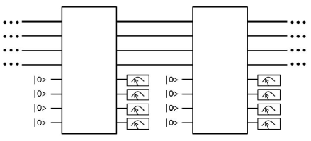
(b)

Figure 1: (a) Comprehensive mechanical measurement on a biological cell in our gedankenexperiment. A number of force/displacement sensors (the needle-like objects) are placed on the cell (the smooth object on the substrate). The substrate may have to incorporate many sensors as well. (b) A quantum circuit model of the cell. The lower portion of the qubits, corresponding to the degrees of freedom on the cell surface, are constantly measured (measurements are represented by the meter objects) and reset to the state $|0\rangle$. The upper portion, corresponding to the internal degrees of freedom of the cell, is only indirectly accessible from the measurement apparatus, i.e. from the surrounding environment. The boxes contains quantum circuit describing the chaotic time evolution. The number of qubits is arbitrary, but here we show 8 qubits for clarity.

The internal dynamics of the cell — or in terms of the quantum circuit shown in Fig. 1 (b), the circuit structure inside the large box — has to be considered to estimate the amount of information leakage. The reason is simple: For an extreme example, the state of the internal qubits is certainly unobservable if no quantum logic gate connects the internal qubits and the surface qubits. On the other hand, consider an internal qubit A corresponding to a degree of freedom pertaining to a molecule deep inside the cell, which interacts indirectly with a surface qubit Z through a chain of qubits, which roughly represents a chain of molecules that has something akin to nearest-neighbor interactions. Suppose for simplicity that in this chain of qubits $\left\{\mathrm{A,B,C,\cdots Z}\right\}$, the interaction is such that qubit A controls qubit B with the controlled-NOT (CNOT) gate, and then qubit B controls qubit C, and so on, eventually reaching the surface qubit Z. Further suppose that initially the qubit A is in the symmetrically superposed state

$$|\psi_{A}\rangle=\frac{|0\rangle+|1\rangle}{\sqrt{2}},$$ (9)

where $|0\rangle$ and $|1\rangle$ correspond to two localized states of the internal molecule, and the rest of the qubits are in the state $|0\rangle$. Then we eventually get an $n$-qubit GHZ state, on which if a measurement on the surface qubit Z is made with respect to the basis $\left\{|0\rangle,|1\rangle\right\}$, then the entire wavefunction collapses. Hence this is the opposite extreme, in which the internal information of the cell is obtainable by measuring the surface molecules. Note that this second situation is at odds with the impossibility hypothesis, except that this particular quantum circuit may not allow for comprehensive internal information acquisition because of the existence of other qubits etc. There are of course cases in between. For example, if each of the above CNOT gate is replaced with a similar gate that rotates the controlled qubit only with a small angle $\varepsilon$ as opposed to the angle $\pi$, the probability amplitude for the state in which the qubit Z is in $|1\rangle$ is approximately $\varepsilon^{N-1}$, where $N$ is the number of qubit in the chain. One may regard this as exponential suppression of information leakage that is fully consistent with the impossibility hypothesis.

Thus, these considerations suggest that detailed knowledge of the biological machinery in the cell is needed to estimate the information leakage rate. However, one may hope go beyond this statement to gain at least a rough estimation without delving into biological details. In the followings we make several crude attempts to this end.

First, we show that the above-mentioned exponential suppression is quite unlikely to happen in the cell for the following reasons. Consider two molecules colliding each other in the cell. Assume for simplicity that these molecules are effectively rigid. If the collision is weak enough to enable the exponential suppression, it should leave the final quantum state of the two molecules largely overlapped with the initial state. This may be seen most clearly by the “caricatured” (in the sense of the word used by Zurek [13]) version appeared above, where the angle-$\varepsilon$ CNOT gate illustrates the weak molecular collision. On the other hand, an actual molecular collision should typically transfer energy of the order of $k_{B}T$ simply because the molecules have such a range of varying energy. However, there are many “energy levels” within the width $k_{B}T$, resulting in a nearly complete change of the quantum state upon collision. (Note that the positional degrees of freedom of the molecule have continuous energy levels. However, they are effectively discretized to the “energy levels” with a spacing $\sim\Delta E$, where the value of $\Delta E$ corresponds to the positional localization length of the molecule.) This is how a version of $\hbar\omega\ll k_{B}T$ comes up here, which is desirable because any discussion lacking emergence of this aspect would be missing an important aspect of large thermal energy. Nevertheless, this shows that the idea of exponential suppression occurring in the cell is most likely to be incorrect.

Since weak collisions between the molecules are unlikely, we need other models of the cell that involves “strong” collisions. First, consider a model, in which neighboring molecules exchange their quantum states upon collision, much like the SWAP gate in a quantum circuit. Hence in this model, a piece of quantum information random walks and hence the information will have leaked when it hits the surface of the cell. When considering this, we imagine localized molecules colliding with each other exchanging their states, which is at odds with another mental picture, in which the molecular positions are delocalized to cause quantum suppression of chaos. Let us ignore this apparent inconsistency and plow ahead. Observe that this whole process is like a random walk, in which changes of the direction are caused by intermolecular collisions. Hence, the “diffusion constant” associated with the process is probably not too different from the actual diffusion constant of biological molecules in a cellular environment. Past measurements [78] have shown that such diffusion constants are roughly in the range of

$$D\cong 10^{-6}\mathrm{cm^{2}/s}=\left(1\mu\mathrm{m}\right)^{2}/\left(10\mathrm{ms}\right).$$ (10)

Another model we consider employs a “random unitary operator” as a single-step discrete time evolution operator. In other words, each big white box in Fig. 1 (b) is such a random unitary operator. We mention a few caveats before we start. First, our definition of the “random unitary operator” $R$ is that the absolute values of all the upper triangular matrix elements and the diagonal matrix elements are independent and identically distributed (i.i.d.) random numbers, while the phases of all upper triangular matrix elements are drawn from the uniform distribution in $[0,2\pi)$. In addition, $R$ of course obeys the unitarity relation $R=R^{\dagger}$. It must be noted that the usual definition of “random unitary operator” is much more sophisticated in order to make certain properties invariant under relevant transformations [79, 80]. However, our discussion is intended only to make a first dent into the problem and hence we do not use advanced concepts. See, e.g. Ref.[81] for an example of more advanced treatment. Second, there are “exponentially many” states in the Hilbert space (although technically the number is uncountable infinity) and hence there are correspondingly many unitary operators that bring $|0\rangle$ to these states. Evidently, most of these unitary operators contain exponentially many quantum logic gates. Therefore, the actual unitary operator that govern cellular time evolution should not be randomly drawn from all the possible unitary operators, but from a “polynomially large” set. We will largely ignore this issue. Third, since the operator is random, our argument ignores geometric structures of the cell. It does not, for instance, take the 3-dimensional nature of the space into account. A randomly distributed nearest-neighbor CNOT gates in a 3-dimensional lattice, for example, would constitute a better model but that is beyond the scope of the present work.

Having mentioned these caveats, we proceed to use the quantum circuit model incorporating the random unitary operator. Note that the general quantum circuit model can describe any quantum system, up to mathematical technicalities. To be specific, let the number of all qubits and the internal qubits in Fig. 1 (b) be $n$ and $m$, respectively. Hence the number of surface qubits is $n-m$. Let $N$ be $N=2^{n}$ and likewise $M=2^{m}$. Basis states are written as $|b_{1}b_{2}\cdots b_{n}\rangle=\bigotimes_{i=1}^{n}|b_{i}\rangle_{i}$, where $b_{i}$, whose value is either $0$ or $1$, represents the value of $i$-th qubit, whose state space is spanned by $|0\rangle_{i}$ and $|1\rangle_{i}$. The label $i$ starts from $1$ to $n$ and points to a surface qubit when $n-m<i$. An alternative way to represent a basis state is $|k\rangle$, where binary representation of the integer $k$ is $b_{1}b_{2}\cdots b_{n}$, so that $0\leq k\leq N-1$. We normalize the state vectors so that $\langle k|l\rangle=\delta_{k,l}$. The complex coefficient of the basis state $|k\rangle$ is written as $c_{k}$. The random unitary operator $R$ representing each big white box in Fig. 1 (b) has matrix elements $R_{k,l}=\langle k|R|l\rangle$. We formulate the problem as follows. Let the first qubit $|b_{1}\rangle_{1}$ represent the internal dynamics of interest, so that $|0\rangle_{1}$ and $|1\rangle_{1}$ represents the position of the molecule under consideration. Suppose that the position of the molecule is already spread due to the chaotic dynamics and hence the state is $\left(|0\rangle_{1}+|1\rangle_{1}\right)/\sqrt{2}$. Furthermore, without loss of generality, we set all other qubit in the state $|0\rangle_{i}$, where $i=2,3,\cdots,n$. To avoid excessive complexity in our analysis, assume that all qubits are disentangled at the beginning. Let the encoding, or mapping, of the molecular quantum states into the qubit states be such that the state $\bigotimes_{i=2}^{n}|0\rangle_{i}$ translates to having a molecular quantum state that is in accordance with the conventional wisdom — that all molecules except the one described by $\left(|0\rangle_{1}+|1\rangle_{1}\right)/\sqrt{2}$ are localized classically and these are not quantum mechanically entangled. Hence, the quantum state we initially have is

$$|\varPsi\rangle=c_{0}|00\cdots 0\rangle+c_{1}|10\cdots 0\rangle,$$ (11)

where $c_{0}=c_{1}=1/\sqrt{2}$. This is a superposition of the positional states of the molecule being at two different places. Here we ignore the apparent inconsistency that only one molecule is delocalized in the crowded cellular environment. The question is how well this superposition of equal amplitude is preserved after a single step of time evolution and a measurement on the surface qubits. We apply the unit-time-step evolution operator $R$ to Eq.(11) to obtain

$$\frac{R_{0,0}|0\rangle+R_{1,0}|1\rangle+R_{2,0}|2\rangle+\cdots}{\sqrt{2}}+\frac{R_{0,1}|0\rangle+R_{1,1}|1\rangle+R_{2,1}|2\rangle+\cdots}{\sqrt{2}},$$ (12)

where the first term represents the state evolved from the first term in Eq.(11) and likewise for the second term. A measurement on all $n-m$ surface qubits results in only $M$ remaining terms in the numerator of each term. Up to a normalization factor, we have

$$|A\rangle+|B\rangle=\left\{R_{X,0}|X\rangle+R_{X+1,0}|X+1\rangle+R_{X+2,0}|X+2\rangle+\cdots\right\}$$

$$+\left\{R_{X,1}|X\rangle+R_{X+1,1}|X+1\rangle+R_{X+2,1}|X+2\rangle+\cdots\right\},$$ (13)

where $X$ depends on the measurement outcome and the states $|A\rangle,|B\rangle$ represent respectively the right-hand-side terms in the first and second set of braces. There are several points to consider. The first point is about the orthogonality between the states $|A\rangle$ and $|B\rangle$. Since the matrix $R_{k,l}$ is “random”, we first make an overall normalization to the matrix so that the average of the square of the absolute value is $\left\langle|R_{k,l}|^{2}\right\rangle\approx 1/M$. Hence $|A\rangle$ and $|B\rangle$ have approximately the unit length. We obtain $|\langle A|B\rangle|\cong 1/\sqrt{M}$ unless $R_{k,l}$ obeys an unusual probability distribution, because the summation goes in the “random walk” fashion due to the random phase of $R_{k,l}$. Hence, $|A\rangle$ and $|B\rangle$ are approximately orthogonal. The second point is how well the equality of the probability amplitudes of $|A\rangle$ and $|B\rangle$ is preserved. This depends on the probability distribution, to which $R_{k,l}$ obeys. For example, if $|R_{k,l}|=1/\sqrt{M}$ holds exactly and $R_{k,l}$ only have random phases, the equality of the amplitudes of $|A\rangle$ and $|B\rangle$ is preserved perfectly. In general, the equality of the probability amplitudes is preserved approximately, again unless $R_{k,l}$ obeys an unusual probability distribution. The third point is whether the relative phase between $|A\rangle$ and $|B\rangle$ is preserved. As can be verified easily, the relative phase is not preserved at all. It is unclear if such an introduction of random phase affects the quantum suppression of chaos. This circumstance resembles to, if we take an analogy from condensed matter physics, e.g. a coherent electron wave under a fluctuating external magnetic field, as opposed to a dissipative motion of the electron that gets entangled with the lattice degrees of freedom. The reason is that the states $|A\rangle$ and $|B\rangle$ remain largely coherent and do not evolve into a mixed state despite the phase noise.

Although the above analysis seems to support the notion that the information leakage is small, this result should be taken with a grain of salt. First, the random unitary operator which brings all states to all states in one time step is not at all realistic. The real-world time-evolution is likely to be sparse with respect to a suitable basis. Second, the above results, such as the difference in probability amplitudes between $|A\rangle$ and $|B\rangle$, depend only on $M$ and not on $N$. This unacceptable aspect comes probably from the fact that we used a rudimentary definition of “random unitary matrix”. Moreover, our analysis does not give us an actual time scale. It appears natural to take roughly the time scale of an inverse Lyapunov exponent to carry out the single time evolution by the operator $R$. However, we do not know the values of such relevant Lyapunov exponents, or how many of them exists, let alone the question of whether they exist at all.

3.4 Quantum suppression of chaos

In view of the above difficulty in estimating the information leakage rate, it is even more difficult to estimate how the suppression of chaos in the cell might play out. Hence we will be brief. We continue to assume that the dynamics of the cell is classically chaotic and that the information leakage rate determines how the quantum state of the cell collapses. The process is, in a sense, competition between the chaotic expansion of the quantum state in the positional space, which occurs with the rate proportional to characteristic Lyapunov exponents, and the collapse of the quantum state by external observations that occurs with the rate that is essentially proportional to the information leakage rate. As mentioned above, we do not know how many unstable degrees of freedom exist in the classical model of a biological cell, nor the various positive Lyapunov exponents associated to these degrees of freedom. A preliminary study could start once these are more or less known. Then we might model the process of “external observation” by collapsing one randomly-selected degree of freedom, for example, setting the “spread of the wave function” (SWF) associated with the degree of freedom to the initial value. When the SWF reaches its maximum value, which will be referred to as the “range” below, we may regard that as beginning of quantum suppression of chaos [13].

To see the crudest physics, consider a simplified system, in which all the positive Lyapunov exponents $\lambda_{i}$ and the range $L_{i}$ of the associated dynamical variables $x_{i}$ are the same for all $N$ unstable degrees of freedom. Hence $\lambda_{i}=\lambda$ and $L_{i}=L$ for all $i=1,2,\cdots,N$. Simplifying even further, the equations of motion that we consider is a set of independent differential equations

$$\dot{y}_{i}=\lambda y_{i},$$ (14)

where $y_{i}$ is roughly the SWF associated with the $i$-th degree of freedom. (For example, the $x_{i}$-dependence of the wavefunction at some given time may approximately be $\simeq e^{-x_{i}^{2}/2y_{i}^{2}}$.) Hence we have $y_{i}=y_{0}e^{\lambda t}$, where $t$ measures the elapsed time since the last wavefunction collapse and $y_{0}$ is the characteristic size of the wavefunction right after the collapse. Note that the wavefunction spreads fully in the allowed range $L$ of the variable $x_{i}$ at $t=t_{L}\cong\left(1/\lambda\right)\ln\left(L/y_{0}\right)$ and the suppression of chaos begins. Note the insensitivity of $t_{L}$ on $L$ and $y_{0}$. Suppose that each degree of freedom is “measured” with a time interval $\Delta\tau$. Then we see that it is a sort of “speed competition” between the exponentially expanding SWF and its collapse caused by the external observations. We might conjecture that this speed competition results in two phases in general, such that the chaotic expansion dominates in one phase ($t_{L}\ll\Delta\tau$) while measurement-induced collapses dominate in the other ($t_{L}\gg\Delta\tau$), depending on the rate of the external observation $\Delta\tau^{-1}$.

3.5 Possible places to find experimental evidence

It is rather easy to imagine a highly conclusive experimental proof for large-scale quantumness in a biological system. However, at present we are not able to propose an experimental scheme that has a non-zero chance to generate evidence for/against quantum suppression of chaos in a biological cell with a reasonable degree of certainty. Hence, we content ourselves with considering where we might find at least circumstantial evidence.

First, there may be thermodynamic evidence. Recall that von Neumann entropy does not increase in an isolated quantum system, even in a system apparently out of equilibrium [82]. This apparent paradox is resolved when interaction with the environment is taken into account. In a usual system, the positional degrees of freedom is subject to einselection, i.e, environment-induced superselection. Hence, the exponential spread of the state in a chaotic system is reflected as a linear increase of entropy as far as the system is observed frequently enough. This process is obviously affected if quantum suppression of chaos is at work in the cell. We check some numbers: Human body comprising $\sim 10^{13}$ cells [83] produces heat flux on the order of $100\mathrm{W}$, suggesting that each cell produces $\dot{Q}\cong 10\mathrm{pW}$ of heat flux. From the relationship

$$dQ=TdS=k_{B}T\cdot d\left(\ln W\right)=0.69k_{B}T\cdot d\left(\log_{2}W\right),$$ (15)

where $S$ is entropy, we can compute how many bits of uncertainty are produced in a cell per unit time as

$$\frac{d\left(\log_{2}W\right)}{dt}=\frac{\dot{Q}}{0.69k_{B}T}\cong 10^{9}\mathrm{bit/s},$$ (16)

where $T=300\mathrm{K}$. If the size of a cell is roughly $\left(1\mu\mathrm{m}\right)^{3}$, then the above calculation suggests that 1 bit of uncertainty, or chaotic spread by a factor $2$ in our picture, is generated in a volume $\left(1\mathrm{nm}\right)^{3}$ every second. For instance, if this rate turns out to be too small for the supposedly chaotic molecular motions in the cell, this number would support the hypothesis that quantum suppression of chaos is going on in the cell. However, all this depends on how many chaotic degrees of freedom there are and what Lyapunov exponents are associated to these. Hence further investigations into the classical dynamics in the cell are desired.

The reader might feel that the concept of quantum suppression of chaos is too eagerly invoked in the above, when heat is simply generated from another form of energy. As a sanity check, consider a light bulb and see how many bits of uncertainty is produced per unit time, similar to the above calculation. We indeed obtain, from the value of heat flux $\dot{Q}$, the number of bits that a single tungsten atom contributes:

$$\frac{d\left(\log_{2}W\right)}{dt}=\frac{\dot{Q}}{0.69k_{B}T}=\frac{\rho\Delta V}{0.69k_{B}T}\left(\frac{I}{\pi d^{2}/4}\right)^{2}\cong 10^{2}\mathrm{bit/s},$$ (17)

(where $T=10^{3}\mathrm{K}$, the tungsten wire diameter is $d=50\mathrm{\mu m}$, the resistivity is $\rho=25\mathrm{\mu\Omega\cdot cm}$, the volume-per-atom is $\Delta V=1.6\times 10^{-29}\mathrm{m^{3}}$ and the current is $I=1\mathrm{A}$.) This number has nothing to do with the chaotic spread of a wavefunction. Instead, it reflects the following situation: The “motion” of a tungsten atom is excited by the electric current, thus having more quantum states available. Then the atom releases heat to the environment, with which “uncertainty” is thrown away because a smaller number of quantum states are available for the tungsten atom after releasing heat. In the case of chaotic systems, the entropy increase due to the spread of wavefunction is understood only in terms of interaction with the environment, that converts the initially pure state (for the sake of argument, imagine that we measured the state of the system before the wavefunction spread) to a mixed state. Hence it is natural to consider that the measurement process itself injects the necessary energy to the chaotic degree of freedom. In the biological cell under our hypothesis, this energy comes presumably from internal degrees of freedom that “monitors” the chaotic degree of freedom. Eventually, the heat must be released to the environment surrounding the cell. Also recall that, at the same time, we put forward the notion that there are not many degrees of freedom that monitor the putative chaotic degrees of freedom. Hence, under this notion, the time for the wavefunction spread is sufficiently long that quantum suppression of chaos can set in. In other words, the “monitoring” mentioned above occurs infrequently enough so that the heat generation is suppressed.

Second, if functioning of the cell, or functioning of life more broadly, critically depends on quantum suppression of chaos, then classical simulations, e.g. MD simulation, of biological cell should fail. A difficulty with this “approach” is that there should be myriad of other things that could make simulations fail. Conversely, falsification of the existence of quantumness in the cell, providing that is the case, would be relatively straightforward by successful classical simulations. On a related note, RCSP described in Sec. 2.1 “classicalizes” the system at each time step separated by $\Delta t$ and this is in a sense similar to classical simulation. Hence, RCSP should also fail to reproduce biologically informative time evolution under the hypothesis that quantum suppression of chaos is at work in the cell.

4 Conclusions and afterthoughts

We started our study by evaluating the impossibility hypothesis, which asserts the fundamental impossibility of a certain type of comprehensive imaging (i.e. CMRV) of the living cell. We were then led to the unusual notion of the possible existence of quantum mechanically delocalized molecules in the biological cell because of the lack of quantum mechanical monitoring, which in turn brought us to the notion of quantum suppression of the putative classical chaos in the biological cell. Our study did not find solid evidence supporting these ideas. Our rather weak conclusion only says that we currently do not know if such a quantum effect exists. Nonetheless, we obtained the following two findings. First, we found that the question about the existence of delocalized molecules in the cell is worth asking at all. In fact, this question has hardly been asked before. Second, we found that answering this question is hard. This is a non-trivial finding because the answer is obvious according to the conventional wisdom, which says all molecules are localized in the cell.

The present study is built on quantum chaology research, in which it is known that even huge objects can evolve into a quantum mechanically smeared state if the system is classically chaotic, and if the system is not observed (i.e. without decoherence). We argued that experience shows that it is difficult, or perhaps impossible, to measure the internal states of the cell comprehensively, real time, at molecular resolution and in true 3D. This suggests that external observers cannot observe some internal states of the cell. We argued that in the cell, unlike other chaotic systems that have been studied, it could be that there are not many non-chaotic degrees of freedom that acts effectively as an internal observer. The reason is that the cell could be a microscopic molecular machine without many extraneous degrees of freedom. We argued that, if that is the case, the chaotic, exponential spreading of wavefunction may outpace the rate at which decoherence effects “collapse” the wavefunction. We argued that, in spite of the short wevelength of the matter wave and the physiological temperature involved, quantum effects, if they exist, could manifest itself through the known phenomenon of quantum suppression of otherwise classically chaotic dynamics. We showed that, if the phenomenon is actually there, it might leave its fingerprints in some places although none of the suggested “fingerprints” are conclusive.

We reiterate the above summary, this time from another viewpoint of how the biological cell, a warm-and-wet physical system, could evade various mechanisms of the emergence of classicality. The first mechanism of the emergence of classicality is similar to how ray optics emerges from wave optics, making the position of an object well-defined. In our case, however, a quantum wavepacket could spread fast enough because of the putative chaotic dynamics. The spread of wavepacket in turn causes interference eventually, despite the fact that the de Broglie wavelengths of molecules are far shorter than the length scale associated with the potential. The second mechanism works when energy associated with the system, such as $k_{B}T$, is sufficiently large to obscure individual energy quanta $\hbar\omega$. However, it is known in quantum chaology that quantum effects manifest itself even when the energy of an object is very large and the associated de Broglie wavelength is short, if the object is well-isolated. This brings us to the third mechanism of decoherence. We argued that if there are a sufficient number of chaotic degrees of freedom in the volume of the cell, information about the motion of these degrees of freedom may not leak out effectively because of the limited surface area of the cell. This could make the degrees of freedom somewhat isolated, which is a prerequisite for the suppression of decoherence.

Before moving on to considerations on possible consequences of the quantumness we have been discussing, we consider a couple of alternative scenarios. First, it should be pointed out that chaotic dynamics is not the only way to amplify quantum uncertainty, or to spread the wavepacket. As exemplified by the Schrodinger’s cat argument, sensitive measurement apparatus can play a similar role. Dynamics of the cell could simulate chaotic dynamics if some molecular systems in the cell effectively act as sensitive quantum measurement apparatus. Note that, however, technically such a system would not necessarily be chaotic in the strict sense because chaoticity requires exponential divergence of classical trajectories at essentially everywhere. Nonetheless, such strict chaoticity is not required in the argument presented in this paper. Second, it could be that CMRV is impossible not because there is no information leaking out. Instead, it might be that the leaked information is hopelessly jumbled up at the cell surface and “reconstruction” of the desired information is next to impossible. If this is the case, quantum coherence needed for the quantum suppression of chaos does not exist. At the same time, this possibility would raise the hope that CMRV is possible after all, perhaps using massive computing power. However, it should be mentioned that this scenario appears to be at odds with the “scaling” idea that the surface area may not be large enough to transmit information arising from the number of “chaotic information sources” that is presumably proportional to the volume, as the system size increases. Nonetheless, it may be that chaotic information sources are not independent but entangled to each other, so that their number is not proportional to the volume.

We next consider possible consequences of the truth or falsehood of the hypothesis that molecules are delocalized in the cell. If it turns out that all molecules in the cell are well-localized as the conventional wisdom states, then there will be no change in our conception of biological systems. Things may have to be reconsidered, however, if it turns out that some molecules are delocalized and quantum suppression of chaos is at work. For example, future research programs of simulating the whole cell by MD simulation will have to take this effect into account, or at least keep the effect in mind. It is currently unknown whether the quantum-mechanically suppressed chaotic systems can be efficiently simulated with a classical computer. If it is impossible to classically simulate such systems efficiently, that might represent an obstacle in the field of computational biomodeling. On the “brighter” side, such impossibility will make quantum computing research more relevant to life science than it already is. More speculatively, future artificial “synthetic biology” systems might perform otherwise intractable computations in this case.

Suppose that the notion appeared in our study — the classically chaotic dynamics of molecules in the cell is suppressed quantum mechanically — is actually true. An interesting question is whether this has direct biological implications, as opposed to implications regarding biology research. In the field of physics of computation, it has been argued that all computations can be done without spending energy, by way of reversible computing [84]. A theoretical example of such a reversible computer is the “billiard ball computer”, in which frictionless motion of colliding classical balls accomplishes any computation without spending energy. There is a caveat, however: The billiard ball computer is extremely sensitive to an external force, internal friction and so on; and its dynamics is essentially chaotic. To make it work, one has to set up feedback systems to measure the positions of the balls, and if a ball goes away from the supposed trajectory, the feedback system should gently push the ball back on the track. However, measurement entails measured data stored in a memory, which eventually need to be discarded. Then, the Landauer-Sagawa-Ueda theorem [85, 86] states that heat must be generated in this whole process of measurement and memory erasure, or in other words entropy must be thrown away. One question associated with this is whether the chaotic motion of a reversible computer can be suppressed quantum mechanically at least partially, thus reducing the reliance on feedback systems. If that is possible, a fascinating question then is whether such a mechanism is at work in biological systems to maintain their “orderly dynamics” without generating excessive heat.

Apart from these speculations, even if the idea studied in this work — the classically chaotic dynamics of molecules in the cell is suppressed quantum mechanically — turns out to be wrong, which definitely is possible, the following idea should be independent from that: There can be a classically chaotic system, which is microscopic in the sense we discussed, whose internal dynamics is highly unobservable from the outside, whose chaotic motion is quantum mechanically suppressed before decoherence sets in, and which operates quantum mechanically outside the traditional domain of quantum systems. Such an engineered system, if built, could find useful applications that might include ultralow-power computing.

References

- [1] G. S. Engel, T. R. Calhoun, E. L. Read, T.-K, Ahn, T, Manoal, Y.-C. Cheng, R. E. Blankenship, and G. R. Fleming. Evidence for wavelike energy transfer through quantum coherence in photosynthetic systems, Nature , 782-786 (2007).
- [2] M. Mohseni, P. Rebentrost, S. Lloyd, and A. Aspuru-Guzik, Environment-assisted quantum walks in photosynthetic energy transfer, J. Chem. Phys. , 174106 (2008).
- [3] T. Ritz, S. Adem, and K. Schulten, A model for photoreceptorbased magnetoreception in birds, Biophys. J. , 707–718 (2000).
- [4] N. Bohr, Light and Life, in: Atomic Physics and Human Knowledge (Dover Book, 2010).
- [5] R. Henderson, The potential and limitations of neutrons, electrons and X-rays for atomic resolution microscopy of unstained biological molecules, Q. Rev. Biophysics, , 171 (1995).
- [6] L. M. Ricciardi and H. Umezawa, Brain and physics of many-body problems, Kybernetik , 44 (1967); M. Jibu and Yasue K, What is mind? Quantum field theory of evanescent photons in brain as quantum theory of consciousness, Informatica. , 471 (1997).
- [7] R. Penrose, Emperor’s New Mind: Concerning Computers, Minds and The Laws of Physics (Oxford University Press, 1989).
- [8] S. Hameroff, Quantum computation in brain microtubules? The Penrose-Hameroff ‘Orch OR’ model of consciousness, Phil. Trans. R. Soc. Lond. A , 1869 (1998), and references therein.
- [9] M. Tegmark, The importance of quantum decoherence in brain processes, Phys. Rev. E , 4194 (2000).
- [10] M. Bordonaro and V. Ogryzko, Quantum biology at the cellular level - elements of the research program, Biosystems , 11 (2013).
- [11] W. Zurek, Pointer basis of quantum apparatus: Into what mixture does the wave packet collapse?, Phys. Rev. D , 1516 (1981).
- [12] W. H. Zurek, Decoherence and the transition form quantum to classical, Physics Today, pp.36, October (1991).
- [13] W. H. Zurek, Decoherence, chaos, quantum–classical correspondence, and the algorithmic arrow of time, Phys. Scri. T , 186 (1998); M. V. Berry, Chaos and the semiclassical limit of quantum mechanics (Is the moon there where somebody looks?), In: R. J. Russell, P. Clayton, K. Wegter-McNelly and J. Polkinghorne (eds.) Quantum mechanics: Scientific perspectives on Divine Action, pp. 41, Vatican Observatory – CTNS Publications (2001).
- [14] A. Sakdinawat and D. Attwood, Nanoscale X-ray imaging, Nature Photon. , 840 (2010).
- [15] J. C. Solem and G. C. Baldwin, Microholography of living organisms, Science. , 229 (1982).
- [16] R. Neutze, R. Wouts, D. van der Spoel, E. Weckert, and J. Hajdu, Potential for biomolecular imaging with femtosecond X-ray pulses, Nature , 752 (2000).
- [17] J. M. J. Madey, Stimulated emission of bremsstrahlung in a periodic magnetic field, J. Appl. Phys. , 1906 (1971).
- [18] D. Sayre, Some implications of a theorem due to Shannon, Acta Cryst. , 843 (1952).
- [19] J. Miao, P. Charalambous, J. Kirz and D. Sayre, Extending the methodology of X-ray crystallography to allow imaging of micrometre-sized non-crystalline specimens, Nature , 342 (1999).
- [20] J. Miao, T. Ishikawa, I. K. Robinson, and M. M. Murnane, Beyond crystallography: Diffractive imaging using coherent x-ray light sources, Science , 530 (2015).
- [21] M. Mutzafi, Y. Shechtman, Y. C. Eldar, O. Cohen, and M. Segev, Sparsity-based ankylography for recovering 3D molecular structures from single-shot 2D scattered light intensity, Nat. Commun. , 7950 (2015).
- [22] H. Okamoto, Quantum interface to charged particles in a vacuum, Phys. Rev. A , 053805 (2015).
- [23] R. Alkofer, M. B. Hecht, C.D. Roberts, S.M. Schmidt, and D.V. Vinnik, Pair creation and an X-ray free electron laser, Phys. Rev. Lett. , 193902 (2001); See also Eq.(13) in: A. Ringwald, Pair production from vacuum at the focus of an X-ray free electron laser, Phys. Lett. , 107 (2001), where one sees that the pair production is basically absent below the Schwinger limit .
- [24] L. Hughes, C. Hawes, S. Monteith, and S. Vaughan, Serial block face scanning electron microscopy—the future of cell ultrastructure imaging, Protoplasma , 395 (2014).
- [25] R. M. Glaeser and K. A. Taylor, Radiation damage relative to transmission electron microscopy of biological specimens at low temperature: a review, J. Microsc. , 127 (1978).
- [26] M. Adrian, J. Dubochet, J. Lepault, and A. W. McDowall, Cryo-electron microscopy of viruses, Nature (London) , 32 (1984).
- [27] M. Haider, H. Rose, S. Uhlemann, B. Kabius, and K. Urban, Towards 0.1 nm resolution with the first spherically corrected transmission electron microscope, J. Electron Microsc. , 395 (1998).
- [28] O.L. Krivanek, N. Dellby, and A.R. Lupini, Towards sub-0.5A electron beams, Ultramicroscopy , 1 (1999).
- [29] O. Scherzer, Spharische und chromatische korrektur von elektronenlinsen, Optik , 114 (1947).
- [30] M. Koshino, T. Tanaka, N. Solin, K. Suenaga, H. Isobe, and E. Nakamura, Imaging of single organic molecules in motion, Science , 853 (2007).
- [31] T. Sasaki, H. Sawada, F. Hosokawa, Y. Kohno, T. Tomita, T. Kaneyama, Y. Kondo, K. Kimoto, Y. Sato, and K. Suenaga, Performance of low-voltage STEM/TEM with delta corrector and cold field emission gun, J. Electron Microsc. , S7 (2010).
- [32] N. Delby, N. Bacon, P. Hrncirik, M. Murfitt, G. Skone, Z. Szilagyi, and O. Krivanek, Dedicated STEM for 200 to 40 keV operation, Eur. Phys. J. Appl. Phys. , 33505 (2011).
- [33] U. Kaiser, J. Biskupek, J.C. Meyer, J. Leschner, L. Lechner, H. Rose, M. Stoger-Pollach, A.N. Khlobystov, P. Hartel, H. Muller, M. Haider, S. Eyhusen, and G. Benner, Transmission electron microscopy at 20 kV for imaging and spectroscopy, Ultramicroscopy , 1239 (2011).
- [34] R. M. Glaeser, K. Downing, D. DeRosier, W. Chiu, and J. Frank, Electron Crystallography of Biological Macromolecules (Oxford University Press, New York, 2007).
- [35] R. M. Glaeser, How good can cryo-EM become? Nat. Methods , 28 (2016).
- [36] A. Elitzur and L. Vaidman, Quantum mechanical interaction-free measurements, Found. Phys. , 987 (1993).
- [37] P. Kwiat, H. Weinfurter, T. Herzog, A. Zeilinger, and M. A. Kasevich, Interaction-free measurement, Phys. Rev. Lett. , 4763 (1995).
- [38] W. P. Putnam and M. F. Yanik, Noninvasive electron microscopy with interaction-free quantum measurements, Phys. Rev. A , 040902(R) (2009).
- [39] G. Mitchison, S. Massar, and S. Pironio, Absorption-free discrimination between semitransparent objects, Phys. Rev. A , 022110 (2002).
- [40] H. Okamoto, Possible use of a Cooper-pair box for low-dose electron microscopy, Phys. Rev. A , 043810 (2012).
- [41] H. Okamoto and Y. Nagatani, Entanglement-assisted electron microscopy based on a flux qubit, Appl. Phys. Lett. , 062604 (2014).
- [42] L. Ciobanu and C.H. Pennington, 3D micron-scale MRI of single biological cells, Solid State Nucl. Magn. Reson. , 138 (2004).
- [43] J. A. Sidles, Noninductive detection of single-proton magnetic resonance, Appl. Phys. Lett. , 2854 (1991).
- [44] D. Rugar, C. S. Yannoni, and J. A. Sidles, Mechanical detection of magnetic resonance, Nature , 563 (1992).
- [45] C. L. Degen, M. Poggio, H. J. Mamin, C. T. Rettner, and D. Rugar, Nanoscale magnetic resonance imaging, Proc. Nat. Acad. Sci. U.S.A. , 1313 (2009).
- [46] C. L. Degen, Scanning magnetic field microscope with a diamond single-spin sensor, Appl. Phys. Lett. , 243111 (2008); J. R. Maze, P. L. Stanwix, J. S. Hodges, S. Hong, J. M. Taylor, P. Cappellaro, L. Jiang, M. V. Gurudev Dutt, E. Togan, A. S. Zibrov, A. Yacoby, R. L. Walsworth, M. D. Lukin, Nanoscale magnetic sensing with an individual electronic spin in diamond, Nature , 644 (2008).
- [47] M. Poggio and C. L. Degen, Force-detected nuclear magnetic resonance: Recent advances and future challenges, Nanotechnology , 342001 (2010).
- [48] Oleg N. Antzutkin, Molecular structure determination: Applications in Biology, pp. 280-390, Chap. 7 in Melinda J. Duer Ed. Solid State NMR Spectroscopy: Principles and Applications, (Wiley, 2007).
- [49] L. Trifunovic, F. L. Pedrocchi, S. Hoffman, P. Maletinsky, A. Yacoby, and D. Loss, High-efficiency resonant amplification of weak magnetic fields for single spin magnetometry at room temperature, Nature Nanotechnology , 541 (2015).
- [50] L. Gross, F. Mohn, N. Moll, P. Liljeroth, and G. Meyer, The chemical structure of a molecule resolved by atomic force microscopy, Science , 1110 (2009).
- [51] N. Kodera, D. Yamamoto, R. Ishikawa, and T. Ando, Video imaging of walking myosin V by high-speed atomic force microscopy, Nature , 72 (2010).
- [52] B. Huang, M. Bates, and X.-W. Zhuang, Super resolution fluorescence microscopy, Annu. Rev. Biochem. , 993 (2009).
- [53] E. Betzig, Nobel lecture: Single molecules, cells, and super-resolution optics, Rev. Mod. Phys. , 1153 (2015).
- [54] M. A. Taylor, J. Janousek, V. Daria, J. Knittel, B. Hage, H.-A. Bachor, W. P. Bowen. Biological measurement beyond the quantum limit, Nat. Photon. , 229 (2013).
- [55] T. Ono, R. Okamoto, and S. Takeuchi, An entanglement-enhanced microscope, Nat. Commun. , 2426 (2013).
- [56] E. A. Ash and G. Nicholls, Super-resolution aperture scanning microscope, Nature , 510 (1972).
- [57] J. B. Pendry, Negative refraction makes a perfect lens, Phys. Rev. Lett. , 3966 (2000).
- [58] See: V. A. Podolskiy and E. E. Narimanov, Near-sighted superlens, Opt. Lett. , 75 (2005) and references therein.
- [59] F. Chen, P. W. Tillberg, and E. S. Boyden, Expansion microscopy, Science , 543 (2015). A video presenting the intention of expansion microscopy is played in: E. Boyden, A new way to study the brain’s invisible secrets, TED talk, TEDSummit (2016).
- [60] O. V. Mosin and I. Ignatov, Studying of isotopic effects of heavy water in biological systems on example of prokaryotic and eukaryotic cells, Biomedicine , 31 (2012).
- [61] J. F. Thomson, Physiological effects of in mammals. Deuterium isotope effects in chemistry and biology, Ann. N. Y. Acad. Sci. , 736–744 (1960).
- [62] M. M. Cox and J. R. Battista, Deinococcus radiodurans — the consummate survivor, Nat. Rev. Microbiol. , 882 (2005).
- [63] M. Arndt, O. Nairz, J. Vos-Andreae, C. Keller, G. van der Zouw, and A. Zeilinger, Wave-particle duality of molecules, Nature , 680 (1999).
- [64] N. Sim, M.-F. Cheng, D. Bessarab, C. M. Jones, and L. A. Krivitsky, Measurement of photon statistics with live photoreceptor cells, Phys. Rev. Lett. , 113601 (2012).
- [65] P. Guptasarma, Does replication-induced transcription regulate synthesis of the myriad low copy number proteins of Escherichia coli? Bioessays , 987 (1995).
- [66] G. Matsumoto, K. Aihara, Y. Hanyu, N. Takahashi, S. Yoshizawa, and J. Nagumo, Chaos and phase locking in normal squid axons, Phys. Lett. A , 162 (1987).
- [67] D. Oliver, A chaotic pendulum, Phys. Teach. , 174 (1999).
- [68] T. Matsumoto, A Chaotic Attractor from Chua’s Circuit, IEEE Trans. Circuits Sys. , 1055 (1984).
- [69] G. Ling, What Determines the Normal Water Content of a Living Cell? Physiol. Chem. Phys. and Med. NMR , 1 (2004).
- [70] R. Feistel and W. Wagner, A comprehensive Gibbs thermodynamic potential of ice, 14th Int. Conf. Properties Water Steam, Kyoto (2004); National Institute of Standards and Technology, A gateway to the data collections. Available at http://webbook.nist.gov (accessed 15 September 2016). We note a useful website on the subject: M. Chaplin, Water structure and science, http://www1.lsbu.ac.uk/water/water_properties.html (accessed 15 September 2016).
- [71] A. I. Kolesnikov, G. F. Reiter, N. Choudhury, T. R. Prisk, E. Mamontov, A. Podlesnyak, G. Ehlers, A. G. Seel, D. J. Wesolowski, and L. M. Anovitz, Quantum tunneling of water in beryl: A new state of the water molecule, Phys. Rev. Lett. , 167802 (2016).
- [72] V. I. Sbitnev, Quantum consciousness in warm, wet, and noisy brain, arXiv:1606.00258 (2016).
- [73] L. A. Rozema, J. D. Bateman, D. H. Mahler, R. Okamoto, A. Feizpour, A. Hayat, and A. M. Steinberg, Scalable spatial superresolution using entangled photons, Phys. Rev. Lett. , 223602 (2014); M. Tsang, Quantum Imaging beyond the Diffraction Limit by Optical Centroid Measurements, Phys. Rev. Lett. , 253601 (2009).
- [74] Y. Takaku, H. Suzuki, I. Ohta, D. Ishii, Y. Muranaka, M. Shimomura, and T. Hariyama, A thin polymer membrane, nano-suit, enhancing survival across the continuum between air and high vacuum, Proc. Natl. Acad. Sci. USA. , 7631 (2012).
- [75] C. Errico, J. Pierre, S. Pezet, Y. Desailly, Z. Lenkei, O. Couture, and M. Tanter, Ultrafast ultrasound localization microscopy for deep super-resolution vascular imaging, Nature , 499 (2015).
- [76] B. Hadimioglu and J. S. Foster, Advances in superfluid helium acoustic microscopy, J. Appl. Phys. , 1976 (1984).
- [77] R. A. Harris, D. H. Follett, M. Halliwell, and P. N. Wells, Ultimate limits in ultrasonic imaging resolution, Ultrasound Med. Biol. , 547 (1991).
- [78] M. J. Saxton, Wanted: scalable tracers for diffusion measurements, J. Phys. Chem. B , 12805 (2014).
- [79] F. Dyson, Statistical theory of the energy levels of complex systems I, J. Math. Phys. , 140 (1962).
- [80] K. Zyczkowski and M. Kus, Random unitary matrices, J. Phys. A: Math. Gen. , 4235 (1994).
- [81] S. Boixo, S. V. Isakov, V. N. Smelyanskiy, R. Babbush, N. Ding, Z. Jiang, J. M. Martinis, and H. Neven, Characterizing quantum supremacy in near-term devices, arXiv:1608.00263 (2016).
- [82] J. Goold, M. Huber, A. Riera, L. del Rio, and P. Skrzypczyk, The role of quantum information in thermodynamics — a topical review, J. Phys. A: Math. Theor. , 143001 (2016).
- [83] E. Bianconi, A. Piovesan, F. Facchin, A. Beraudi, R. Casadei, F. Frabetti, L. Vitale, M. C. Pelleri, S. Tassani, F. Piva, S. Perez-Amodio, P. Strippoli, and S, Canaider, An estimation of the number of cells in the human body, Ann. Hum. Biol. , 463 (2013).
- [84] Sec. 3.2.5 Energy and Computation, in: M. A. Nielsen and I. L. Chuang, Quantum computation and quantum information (Cambridge University Press, 2000).
- [85] R. Landauer, Irreversibility and heat generation in the computing process, IBM J. Res. Dev. , 183 (1961).
- [86] T. Sagawa and M. Ueda, Minimal energy cost for thermodynamic information processing: Measurement and information erasure, Phys. Rev. Lett. , 250602 (2009).