One-Dimensional Self-organization and Nonequilibrium Phase Transition in a Hamiltonian System

Abstract

Self-organization and nonequilibrium phase transitions are well known to occur in two- and three- dimensional dissipative systems. Here, instead, we provide numerical evidence that these phenomena also occur in a one-dimensional Hamiltonian system. To this end, we calculate the heat conductivity by coupling the two ends of our system to two heat baths at different temperatures. It is found that when the temperature difference is smaller than a critical value, the heat conductivity increases with the system size in power law with an exponent considerably smaller than 1. However, as the temperature difference exceeds the critical value, the system’s behavior undergoes a transition and the heat conductivity tends to diverge linearly with the system size. Correspondingly an ordered structure emerges. These findings suggest a new direction for exploring the transport problems in one dimension.

Self-organization phenomena SO are ubiquitous in nature and human society. Among others, nonequilibrium phase transitions (NPTs) are a familiar route leading to collective organized behavior NPT . A well-known example is the Rayleigh-Bénard convection RB observed in a horizontal fluid layer heated from below. When the temperature difference between the heater and the thermal sink (set on the fluid layer) is low, the fluid layer is static and the heat is transferred uniformly from bottom to top. But when the temperature difference reaches a critical value, the microscopic random movement spontaneously becomes ordered on a macroscopic level. The fluid spontaneously organizes into a regular pattern of convection cells and the heat flux is dramatically increased compared to the molecular heat conduction. Rayleigh-Bénard convection indicates that a physical system may have the ability to radically change its structure to adaptively respond to strong thermodynamic driving.

These phenomena of self-organization and NPTs are known to take place in two and three dimensions. In the one-dimensional (1D) case instead, despite extensive analytical, numerical, and experimental investigations, they have not been observed yet in any physical systems Lepri14 . A class of systems where 1D NPTs are intensively studied is given by hopping models in which particles hop from one site to another on a 1D lattice with a prescribed stochastic dynamic Evans00 . These models have been found useful in a wide range of applications such as directed percolation, growing interfaces, traffic flows, and so on. They are not suitable, however, to study problems where physical quantities like energy and momentum are involved.

On the other hand, in the past few decades the study of 1D transport problems has attracted considerable interest Lepri03-16 ; Dhar08 ; Lee-Dadswell . A remarkable result states that for a general 1D momentum conserving system, the heat conductivity diverges with the system size in a power law and the diverging exponent may take a universal value under certain conditions Lee-Dadswell ; Narayan ; Lepri0607 ; Beijeren12 ; Spohn13 . It is worth noting that a common basis for different theoretical approaches is the linear response theory that is valid near equilibrium. Therefore, NPTs, which usually occurs far from equilibrium, have been implicitly excluded.

In this Letter we show that NPT and self-organization can take place in a 1D Hamiltonian system. Our result also suggests the need to extend the study of 1D transport problems beyond the linear response regime. In principle, this might reveal new mechanisms for energy, momentum, and matter transport.

Our model is a combination of the classical version of the Lieb-Liniger model LL63-1 ; LL63-2 and the two-mass gas model introduced in Ref. Casati86 . It consists of $N$ point particles with short-range interaction, confined in a 1D box of length $L$. The Hamiltonian is

$$H=\sum_{i}\frac{p_{i}^{2}}{2m_{i}}+\sum_{i<j}V(x_{i}-x_{j}),$$ (1)

where $p_{i}$, $m_{i}$, and $x_{i}$ are, respectively, the momentum, mass, and position of the $i$th particle. The mass of a particle is either $\mu_{1}$ or $\mu_{2}$, and the potential $V(x)$ is a step function: $V(x)=h$ for $x\leq|r|$ and $V(x)=0$ otherwise, with $h\geq 0$ being the potential barrier. In this work we consider the limit case $r\to 0$. This case has been considered in Ref. Kurchan02 in order to study the Soret effect which basically consists in a formation of a density gradient when a binary fluid is subjected to a temperature gradient.

According to the Hamiltonian Eq. (1), all particles move freely, and when two particles meet, either they pass through each other without changing their velocities or they collide elastically, depending on their total energy. More precisely, if their total energy in the frame of the center of mass is larger than $h$, or equivalently, if their relative velocity (speed) is larger than a certain value, i.e., $|v_{i}-v_{j}|>\sqrt{2h(m_{i}+m_{j})/(m_{i}m_{j})}$, then the two particles pass through each other; otherwise they collide elastically. Note that the interaction between particles conserves their energy and momentum, and that the limiting case $h=0$ corresponds to particles moving freely and independently while $h=\infty$ corresponds to the standard 1D hard point gas Casati86 . Also note that for a finite $h$ the potential $V(x)$ is symmetric (with respect to $x=0$), but for $h=\infty$, due to the fact that particles do not cross each other, the potential function is in effect asymmetric.

To compute the heat conductivity of the system, we couple its two ends to two heat baths at temperature $T_{L}=T+\Delta$ and $T_{R}=T-\Delta$, respectively. When the first (last) particle of mass $\mu_{i}$ hits the left (right) boundary of the box, it is reflected back with a new velocity $v$ given by the probability distribution Bath :

$$P_{L,R}(v)=\frac{|v|\mu_{i}}{k_{B}T_{L,R}}\exp{(-\frac{v^{2}\mu_{i}}{2k_{B}T_{L,R}})},$$ (2)

where $k_{B}$ is the Boltzmann constant. The heat conductivity is then evaluated as $\kappa=jL/(T_{L}-T_{R})$, with $j$ being the thermal current. Since in our system the heat conductivity follows the scaling $\kappa(cT,c\Delta,ch)=\sqrt{c}\kappa(T,\Delta,h)$, we fix $T$ and investigate the dependence of $\kappa$ on $\Delta$ and $h$. For details of numerical simulation, see Ref. Chen14 . For all data points shown in the figures the errors are at most $3\%$, and as the error bars are smaller than the symbols, they are omitted.

First, we have checked that the results do not qualitatively depend on the particular temperature $T$ and mass values. Therefore, we choose $k_{B}=1$, $T=5$, $N/2$ particles with mass $\mu_{1}=1$ and $N/2$ particles with mass $\mu_{2}=2$. We fix $L=N$ so that, on average, there is one particle in a unit volume (length). We have also verified that the results do not depend on initial conditions; in particular, and quite importantly, as long as $h\neq\infty$, they do not depend on the initial particle-mass configuration either.

For the special, limiting case $h=0$, particles move freely and independently. We therefore have

$$\kappa=N\sqrt{\frac{k_{B}^{3}}{2\pi}}(\frac{1}{\sqrt{\mu_{1}}}+\frac{1}{\sqrt{\mu_{2}}})/(\frac{1}{\sqrt{T_{L}}}+\frac{1}{\sqrt{T_{R}}}).$$ (3)

Up to the first order in $\Delta/T$, $\kappa$ does not depend on $\Delta$, while the second-order correction is only $1.5\%$ for $\Delta/T=0.2$. Hence $\Delta=1$ (with $T=5$) can be considered inside the linear response regime (see Fig. 1). For the opposite limiting case $h=\infty$ numerical simulations provide empirical evidence that $\Delta=1$ is also within the linear response regime. In addition, based on the linear response theory it is predicted that $\kappa\sim N^{1/3}$ in the thermodynamic limit Narayan ; Lepri0607 ; Beijeren12 ; Spohn13 . This result is supported by our numerical simulations as well, which give $\kappa\sim N^{0.30}$ for $10^{3}<N<4\times 10^{4}$. (More simulation results for other mass values of $\mu_{1}$ and $\mu_{2}$ and a bigger temperature difference $\Delta=3$ can be found in Ref. Yang .) In summary, for both limiting cases $h=0$ and $h=\infty$ there is a linear response regime up to $\Delta=1$ in which the heat conductivity does not depend on the temperature difference $\Delta$ significantly.

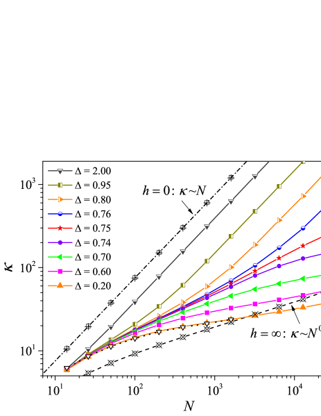
Figure 1: The heat conductivity as a function of the system size for $h=10$ and for several temperature difference values $\Delta>0$. As a comparison, the black open triangles connected by the dotted line segments are for the heat conductivity computed in the equilibrium state (corresponding to $\Delta=0$) by using the Green-Kubo formula Dhar09 . For reference, we show also the case $h=0$ for $\Delta=0.2$ (open squares) and $\Delta=1.0$ (plus signs) and the case $h=\infty$ for $\Delta=0.2$ (open circles) and $\Delta=1.0$ (crosses). The straight dot-dashed line is the result given by Eq. (3) up to the first order of $\Delta/T$.

In clear contrast, for a finite but nonzero value of $h$, the dependence of the heat conductivity on the system size $N$ and on the temperature difference $\Delta$ is completely different. A typical result is shown in Fig. 1 for $h=10$. It can be seen that the dependence of $\kappa$ on $N$ dramatically depends on the temperature difference $\Delta$ and the most striking feature is the existence of a critical value of $\Delta$, $\Delta_{cr}=0.75$, that divides the $N$ dependence of $\kappa$ into two separate classes: For $\Delta>\Delta_{cr}$, $\kappa$ tends to increase linearly with $N$, while for $\Delta<\Delta_{cr}$, $\kappa$ tends to increase with $N$ as $\kappa\sim N^{\alpha}$, with $\alpha\approx 0.17$. At the special value $\Delta$=$\Delta_{cr}$, $\kappa$ tends to increase with $N$ in power law as well but with an exponent of $\alpha\approx 0.50$ instead (see red stars in Fig. 1). It is worth noting that, since the numerical values of $\alpha$ are evaluated based on the simulation results at finite system sizes, one should be very careful in attempting to extrapolate them to the thermodynamic limit, which is, as usual, a delicate question Lepri03-16 .

Figure 2: (a)-(c) The average mass of particles at position $x$, at the stationary state, for the same value $h=10$ as in Fig. 1. (a) $\Delta=0.9>\Delta_{cr}$, (b) $\Delta=0.75=\Delta_{cr}$, and (c) $\Delta=0.6<\Delta_{cr}$, respectively. The corresponding temperature profile is shown in (d)-(f). In all six panels, the orange dotted, the gray dash-dotted, the red dashed, and the blue solid line are, respectively, for the system size $N=1600$, $3200$, $6400$, and $12800$. The green vertical line in (a) indicates the position of the interface of the two species of particles if they are assumed to separate entirely.

We conjecture that $\Delta_{cr}$ is a critical point based on the following two observations. First, the heat conductivity as a function of the system size depends on $\Delta$ very sensitively in the neighborhood of $\Delta_{cr}$; e.g., changing $\Delta$ by just 0.01 away from $\Delta_{cr}$ causes a transition from one class to the other of the dependence $\kappa$ versus $N$ (see the two nearest neighboring curves next to $\Delta_{cr}$ in Fig. 1). This is a strong signal of critical phenomena. Second, the structure of the system at the stationary state is qualitatively different for $\Delta>\Delta_{cr}$ and $\Delta<\Delta_{cr}$. This is illustrated in Fig. 2, where we plot $\overline{m}(x)$, i.e., the average mass of the particles passing a given position $x$. It is interesting to note that for $\Delta>\Delta_{cr}$ [see Fig. 2(a)], the system is characterized by an ordered “sandwich” structure: while heavy particles of mass $\mu_{2}$ aggregate at the hot (left) end, light particles of mass $\mu_{1}$ aggregate at the cold (right) end, and in between there is a transition layer. This layer is characterized by a steep linear center whose width does $not$ change as the system size $N$ increases. Therefore, in the variable $x/N$, the width of the transition layer shrinks to zero as $N$ increases [see Fig. 2(a)]. The vertical line at $x/N=T_{L}/(T_{L}+T_{R})=0.59$ in Fig. 2(a) corresponds to the ideal situation of complete separation of the two species of particles with different masses.

It is interesting to investigate how fast the average particle mass at the left and right ends of the system converge to $\mu_{2}$ and $\mu_{1}$ respectively, for $\Delta>\Delta_{cr}$. Numerical results shown in Fig. 3 (for the left end) indicate the scaling $\mu_{2}-\overline{m}(0)\sim N^{-1.5}$.

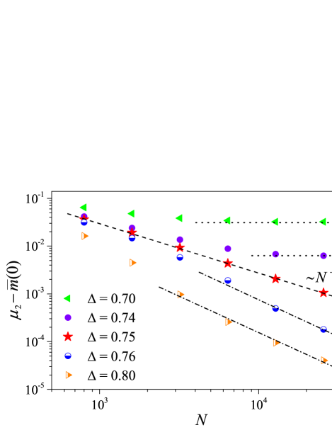
Figure 3: The average particle mass $\overline{m}(0)$ at the leftmost end of the system for $h=10$. The dotted, dashed, and dot-dashed lines indicate, respectively, the scaling $\sim N^{0}$, $\sim N^{-1}$, and $\sim N^{-1.5}$.

The ordered sandwich structure explains satisfactorily the asymptotic scaling $\kappa\sim N$ for $\Delta>\Delta_{cr}$, because increasing the number of particles, or, equivalently, the size of the system, basically only causes the two ending aggregating segments to increase their sizes, but the thermal resistance which is mainly due to the transition layer does not change significantly. As a consequence the heat current does not change significantly either. Accordingly, the temperature profile $T(x)$ also exhibits a sandwich structure: since the particles in the two ending segments are almost identical, no noticeable internal temperature gradient can appear; a temperature gradient is expected only in the transient layer, as is indeed confirmed by the results in Fig. 2(d).

For $\Delta<\Delta_{cr}$, the sandwich structure vanishes: the function $\overline{m}(x)$ for different system sizes agrees with each other almost perfectly upon scaling $x\to x/N$ [Fig. 2(c)] and so does $T(x)$ [Fig. 2(f)]. Quite obviously, as $\Delta$ decreases, the functions $\overline{m}(x)$ and $T(x)$ will become more and more homogeneous till completely uniform at $\Delta=0$. Such a distinctive feature convincingly demonstrates that our system has two different nonequilibrium phases.

At $\Delta=\Delta_{cr}$ [see Fig. 2(b)], both the sandwich and the scaling-invariance features are lost. Here, as $N$ increases, $\overline{m}(x)$ at the two ends of the system still tends to $\mu_{2}$ and $\mu_{1}$. However, quite strikingly, a good and different scaling $\mu_{2}-\overline{m}(0)\sim N^{-1}$ emerges over a wide system size range (Fig. 3), supporting again that $\Delta=\Delta_{cr}$ is a critical point.

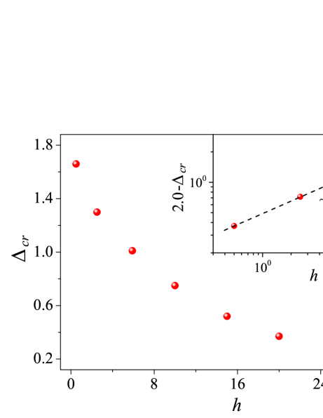
Figure 4: The dependence of the critical temperature difference $\Delta_{cr}$ on the interaction parameter $h$. Inset: Same as the main panel but in log-log scale.

So far we have investigated the case $h=10$. The same critical phenomenon takes place for any finite value of $h>0$ we have considered. Quite obviously, the numerical value of $\Delta_{cr}$ (as well as the exponent $\alpha$ for $\Delta=\Delta_{cr}$) depends on $h$. This is illustrated in Fig. 4, where it is seen that $\Delta_{cr}$ decreases as $h$ increases. This fact may appear counterintuitive at first sight and call into question the mechanism according to which heavy (light) particles tend to reside in the hot (cold) end. The simplest case of two particles, one light and one heavy, may shed some light. In this case, by taking into consideration the dynamics and the heat bath model [see Eq. (2)], it can be shown straightforwardly that the probability for the two particles to cross each other is higher when the light particle is at the hot end than vice versa. This is because the relative velocity (speed) of the two particles is larger when the light particle is at the hot end. In addition, it can be shown further that this asymmetry becomes enhanced as $\Delta$ increases at a fixed $h$, or as $h$ increases at a fixed $\Delta$. This mechanism should also work in a larger system.

Quite clearly, NPT is not present in the limiting cases $h=0$ and $h=\infty$. In the former case particles move independently and the system is integrable, while in the latter case the particles are not allowed to change their order; hence, the mass configuration is determined by the initial setting.

Finally, we have considered so far the case in which the ratio of the two species of particles with different masses is unity. We remark that the NPT properties do not depend on this ratio sensitively. For example, when this ratio is decreased to 2/8 (light to heavy) the value of $\Delta_{cr}$ is still $0.75$ within numerical accuracy.

To summarize, NPT and self-organization have been shown to take place in a 1D Hamiltonian system. It is found that the system can adjust its structure adaptively to respond to the external thermal driving. In particular, for $\Delta>\Delta_{cr}$, an ordered sandwich structure appears, leading to the asymptotic linear dependence $\kappa\sim N$. For $\Delta<\Delta_{cr}$, as the system size increases, the structure of the system tends to be scaling invariant and the heat conductivity tends to increase as the system size in power law with the exponent being considerably smaller than 1.

Importantly, in our system a linear response regime comparable to the cases $h=0$ and $h=\infty$ does not exist. [To be precise, our results do not exclude the existence of a linear response regime in a much narrower range of $\Delta$. For example, for $h=10$, the case we have mainly focused on, a linear response regime may exist within $\Delta<0.2$ (see Fig. 1).] The heat conductivity measured in the nonequilibrium setup depends on $\Delta$ and, hence, is different from that obtained with the Green-Kubo formula by integrating the heat current autocorrelation function in the equilibrium state. The behavior of our model is, therefore, another confirmation that “nonequilibrium is different” Dorfman15 ; Politi11 and calls for a new theoretical approach in dealing with transport problems in systems of similar type.

As it has been shown here, NPT in our 1D system not only manifests itself in the heat conduction behavior but also in the mass distribution. A related significant problem is how NPT and self-organization may influence the 1D matter transport in a physical system. Important practical examples include molecules and micelles translated along tubulous filaments Kral13 . Of particular interest is to investigate the relevance for the coupled heat and particle current which determines thermoelectric power generation and refrigeration Benenti13 ; Benenti16 . This study is in progress.

We acknowledge support by NSFC (Grants No. 11535011, No. 11335006, and No. 11275159), by MIUR-PRIN, and by the CINECA project Nanostructures for Heat Management and Thermoelectric Energy Conversion.

References

- (1) P. Glansdorff and I. Prigogine, Thermodynamic Theory of Structure, Stability and Fluctuations (Wiley-Interscience, London, 1971).
- (2) A. B. H. Haken, Synergetics, An Introduction: Nonequilibrium Phase Transitions and Self-Organization in Physics, Chemistry, and Biology (Springer-Verlag, Berlin, 1978).
- (3) A. V. Getling, Rayleigh-Bénard Convection: Structures and Dynamics (World Scientific, Singapore, 1998).
- (4) S. Iubini, S. Lepri, R. Livi, and A. Politi, Phys. Rev. Lett. 112, 134101 (2014). In this Letter, a 1D boundary-induced NPT has been found which, however, takes place at zero temperature with zero energy current.
- (5) M. R. Evans, Braz. J. Phys. 30, 42 (2000).
- (6) S. Lepri, R. Livi, and A. Politi, Phys. Rep. 377, 1 (2003); Lect. Notes in Phys. 921, 1 (2016).
- (7) A. Dhar, Adv. Phys. 57, 457 (2008).
- (8) G. R. Lee-Dadswell, B. G. Nickel, and C. G. Gray, Phys. Rev. E 72, 031202 (2005); J. Stat. Phys. 132, 1 (2008).
- (9) O. Narayan and S. Ramaswamy, Phys. Rev. Lett. 89, 200601 (2002).
- (10) L. Delfini, S. Lepri, R. Livi, and A. Politi, Phys. Rev. E 73, 060201(R) (2006); J. Stat. Mech. (2007) P02007.
- (11) H. van Beijeren, Phys. Rev. Lett. 108, 180601 (2012).
- (12) C. B. Mendl and H. Spohn, Phys. Rev. Lett. 111, 230601 (2013).
- (13) E. H. Lieb and W. Liniger, Phys. Rev. 130, 1605 (1963).
- (14) E. H. Lieb, Phys. Rev. 130, 1616 (1963).
- (15) G. Casati, Found. Phys. 16, 51 (1986).
- (16) A. Garriga, J. Kurchan, and F. Ritort, J. Stat. Phys. 106, 109 (2002). Actually, an extreme form of the Soret effect, namely, a total phase separation even for arbitrarily small temperature differences, is claimed to take place here.
- (17) J. L. Lebowitz and H. Spohn, J. Stat. Phys. 19, 633 (1978); R. Tehver, F. Toigo, J. Koplik, and J. R. Banavar, Phys. Rev. E 57, 17(R) (1998).
- (18) S. Chen, J. Wang, G. Casati, and G. Benenti, Phys. Rev. E 90, 032134 (2014).
- (19) P. Grassberger, W. Nadler, and L. Yang, Phys. Rev. Lett. 89, 180601 (2002).
- (20) A. Kundu, A. Dhar, and O. Narayan, J. Stat. Mech. (2009) L03001.
- (21) T. R. Kirkpatrick and J. R. Dorfman, Phys. Rev. E 92, 022109 (2015).
- (22) A. Politi, J. Stat. Mech. (2011) P03028.
- (23) P. Král and B. Wang, Chem. Rev. 113, 3372 (2013).
- (24) G. Benenti, G. Casati, and J. Wang, Phys. Rev. Lett. 110, 070604 (2013).
- (25) G. Benenti, G. Casati, K. Saito, and R.S. Whitney, arXiv:1608.05595v1.