Hybrid Quantile Regression Estimation for Time Series Models with Conditional Heteroscedasticity

Abstract

Estimating conditional quantiles of financial time series is essential for risk management and many other applications in finance. It is well-known that financial time series display conditional heteroscedasticity. Among the large number of conditional heteroscedastic models, the generalized autoregressive conditional heteroscedastic (GARCH) process is the most popular and influential one. So far, feasible quantile regression methods for this task have been confined to a variant of the GARCH model, the linear GARCH model, owing to its tractable conditional quantile structure. This paper considers the widely used GARCH model. An easy-to-implement hybrid conditional quantile estimation procedure is developed based on a simple albeit nontrivial transformation. Asymptotic properties of the proposed estimator and statistics are derived, which facilitate corresponding inferences. To approximate the asymptotic distribution of the quantile regression estimator, we introduce a mixed bootstrapping procedure, where a time-consuming optimization is replaced by a sample averaging. Moreover, diagnostic tools based on the residual quantile autocorrelation function are constructed to check the adequacy of the fitted conditional quantiles. Simulation experiments are carried out to assess the finite-sample performance of the proposed approach. The favorable performance of the conditional quantile estimator and the usefulness of the inference tools are further illustrated by an empirical application.

Keywords and phrases: Bootstrap method; Conditional quantile; GARCH; Nonlinear time series; Quantile regression.

1 Introduction

Time series models with conditional heteroscedasticity have become extremely popular in financial applications since the appearance of Engle’s (1982) autoregressive conditional heteroscedastic (ARCH) model and Bollerslev’s (1986) generalized autoregressive conditional heteroscedastic (GARCH) model; see also Francq & Zakoian (2010). These models are widely used in the assessment and management of financial risk, including the estimation of quantile-based measures such as the Value-at-Risk (VaR) and the Expected Shortfall (ES). Spurred by the need of various financial institutions and regulatory authorities, quantile-based measures now play an important part in quantitative analysis and investment decision making. For this reason, estimating conditional quantiles of financial time series is crucial to both academic researchers and professional practitioners in many areas of economics and finance. Furthermore, as conditional quantiles can be directly estimated by quantile regression (Koenker & Bassett 1978), it is especially appealing to study the conditional quantile inference for conditional heteroscedastic models via quantile regression.

Among the large number of conditional heteroscedastic models, arguably the most popular and influential one is Bollerslev’s (1986) GARCH model, since its specification is intuitive, parsimonious and readily interpretable. It has proven highly successful in capturing the volatility clustering of financial time series, and therefore has been frequently integrated into the areas of asset pricing, asset management and financial risk management. The GARCH$(p,q)$ model can be written as

$$x_{t}=\sqrt{h_{t}}\eta_{t},\hskip 14.22636pth_{t}=\alpha_{0}+\sum_{i=1}^{q}\alpha_{i}x_{t-i}^{2}+\sum_{j=1}^{p}\beta_{j}h_{t-j},$$ (1.1)

where $\{\eta_{t}\}$ is a sequence of independent and identically distributed ($i.i.d.$) innovations with mean zero and variance one. Despite the fast-growing interest in conditional quantile inference for time series models (Koenker 2005), the literature on quantile regression for the GARCH model is relatively sparse due to technical difficulties in the estimation. Specifically, consider the conditional quantile of the GARCH process given by (1.1),

$$Q_{\tau}(x_{t}|\mathcal{F}_{t-1})=Q_{\tau,\eta}\sqrt{\alpha_{0}+\sum_{i=1}^{q}\alpha_{i}x_{t-i}^{2}+\sum_{j=1}^{p}\beta_{j}h_{t-j}},\quad 0<\tau<1,$$ (1.2)

where $Q_{\tau,\eta}$ is the $\tau$th quantile of $\eta_{t}$, and $\mathcal{F}_{t}$ is the information set available at time $t$. The square-root function in (1.2), together with the non-smooth loss function in quantile regression, $\rho_{\tau}(x)=x[\tau-I(x<0)]$, leads to a non-smooth objective function which is non-convex even for the ARCH special case. It is this feature that causes the challenges in asymptotic derivation and numerical optimization, and the problem is even more complicated in view of the recursive structure of the conditional variances $\{h_{t}\}$.

On account of these difficulties, the previous literature considered quantile regression estimation for Taylor’s (1986) linear ARCH (LARCH) or linear GARCH (LGARCH) models. In particular, an LGARCH($p,q$) model has the following form,

$$y_{t}=\sigma_{t}\varepsilon_{t},\hskip 14.22636pt\sigma_{t}=\alpha_{0}+\sum_{i=1}^{q}\alpha_{i}|y_{t-i}|+\sum_{j=1}^{p}\beta_{j}\sigma_{t-j},$$ (1.3)

where $\{\varepsilon_{t}\}$ is a sequence of $i.i.d.$ innovations with mean zero. Its conditional quantile has a much simpler form,

$$Q_{\tau}(y_{t}|\mathcal{F}_{t-1})=\left(\alpha_{0}+\sum_{i=1}^{q}\alpha_{i}|y_{t-i}|+\sum_{j=1}^{p}\beta_{j}\sigma_{t-j}\right)Q_{\tau,\varepsilon},\quad 0<\tau<1,$$ (1.4)

where $Q_{\tau,\varepsilon}$ is the $\tau$th quantile of $\varepsilon_{t}$. Koenker & Zhao (1996) first considered the conditional quantile estimation for the LARCH($q$) model, which, without any $\sigma_{t-j}$ involved in (1.4), reduces to a linear quantile regression problem. Quantile regression for the LGARCH model, in contrast, is more troublesome due to the recursive structure of the conditional scales $\{\sigma_{t}\}$. To tackle this, Xiao & Koenker (2009) proposed a two-stage scheme, where they replaced the unobservable $\sigma_{t-j}$’s in (1.4) with some initial estimates first, enabling a linear quantile regression at the second stage. Nevertheless, most practitioners and researchers still prefer Bollerslev’s (1986) GARCH model in (1.1). For this reason, Lee & Noh (2013) studied the asymptotic properties of a quantile regression estimator for the GARCH model, without addressing the feasibility of the numerical optimization for this estimator. For a detailed discussion on the algorithmic issues in quantile regression, see Koenker & Park (1996).

The purpose of this paper is to develop an easy-to-implement approach to the conditional quantile estimation and inference for Bollerslev’s (1986) original GARCH model given by (1.1). To overcome the aforementioned difficulties, we design the following transformation $T:\mathbb{R}\rightarrow\mathbb{R}$ for the conditional quantile in (1.2),

$$T(x)=x^{2}\operatorname*{sgn}(x),$$ (1.5)

where $\operatorname*{sgn}(\cdot)$ is the sign function. Note that there are two desirable properties of $T(\cdot)$:

• it is the inverse of the square-root function in some sense;

• it is continuous and nondecreasing on $\mathbb{R}$.

Owing to this design of $T(\cdot)$, the conditional quantile of the transformed sequence $\{T(x_{t})\}$ resembles that of the LGARCH process $\{y_{t}\}$ in (1.4), in that

$$Q_{\tau}[T(x_{t})|\mathcal{F}_{t-1}]=\left(\alpha_{0}+\sum_{i=1}^{q}\alpha_{i}x_{t-i}^{2}+\sum_{j=1}^{p}\beta_{j}h_{t-j}\right)T(Q_{\tau,\eta}),$$ (1.6)

where $x_{t-i}^{2}=|T(x_{t-i})|$. This connects the conditional quantile inference of the GARCH model directly to that of the LGARCH model. As a result of this connection, we can estimate $Q_{\tau}(x_{t}|\mathcal{F}_{t-1})$ through estimating $Q_{\tau}[T(x_{t})|\mathcal{F}_{t-1}]$. Specifically, we can first estimate $Q_{\tau}[T(x_{t})|\mathcal{F}_{t-1}]$ via linear quantile regression with some initial estimates of $\{h_{t}\}$. Then, by applying the inverse transformation $T^{-1}(\cdot)$ to the estimator of $Q_{\tau}[T(x_{t})|\mathcal{F}_{t-1}]$, we can obtain that of $Q_{\tau}(x_{t}|\mathcal{F}_{t-1})$, owing to the monotonicity of the transformation.

The quantile regression based on (1.6) requires appropriate initial estimates of the conditional variances $\{h_{t}\}$. In Xiao & Koenker (2009), the conditional scales $\{\sigma_{t}\}$ of the LGARCH process (1.3) are estimated based on a sieve approximation of $\sigma_{t}$ with an $m$th-order linear ARCH model: $\sigma_{t}=\gamma_{0}+\sum_{j=1}^{m}\gamma_{j}|y_{t-j}|$, with $m\rightarrow\infty$. A similar sieve approximation may be used on the GARCH model (1.1) based on $h_{t}=\gamma_{0}+\sum_{j=1}^{m}\gamma_{j}x_{t-j}^{2}$. However, the tunning parameter $m$ heavily affects the numerical stability of the procedure: e.g., larger $\alpha_{i}$ and $\beta_{j}$ would require bigger $m$, but unnecessarily large $m$ can introduce too much noise into the estimation; see the Monte Carlo evidence in Section 5.1. On account of this, we estimate $\{h_{t}\}$ by the Gaussian quasi-maximum likelihood estimator (QMLE) for the GARCH model. The asymptotic normality of this estimator under mild technical conditions is established by Francq & Zakoian (2004), and it is easier to implement as well as numerically more stable than the sieve method. Therefore, in this paper, a hybrid conditional quantile estimator for the GARCH model is constructed based on two estimators of different nature: the Gaussian QMLE, which incorporates the global model structure, and the quantile regression estimator, which approximates the conditional quantiles locally.

We derive the asymptotic properties of the proposed estimator and statistics. These limiting results facilitate the statistical inference in this paper. On the other hand, a sparsity/density function enters the asymptotic distribution of the quantile regression estimator, and any feasible inference procedure requires that the density is handled appropriately. Estimation of the density function, although possible, is usually complicated and depends on additional tunning parameters. The preliminary estimation of the density function seriously affects the finite-sample performance of the inference procedures. For this reason, we propose a bootstrap method to approximate the distribution.

Jin et al. (2001) considered a bootstrap method by perturbing the minimand of the objective function with random weights, which is especially useful for time series models as the observations are ordered by time; see also Rao & Zhao (1992), Li et al. (2014) and Zhu (2016). Applying this method to our context, we may conduct a randomly weighted QMLE first, followed by a randomly weighted linear quantile regression. Nonetheless, since the sparsity/density function is not involved in the asymptotic distribution of the QMLE, the first bootstrapping step is actually unnecessary. In view of this, we propose a mixed method: we suggest replacing the first step with a sample averaging, so that the time-consuming optimization need only be performed in the second bootstrapping step. A significant reduction in the computation time hence results.

The asymptotic results and the proposed bootstrap method are useful for conditional quantile inference. For example, the bootstrapping procedure enables us to construct confidence intervals for the fitted conditional quantiles, which may be especially interesting in practice. Furthermore, adopting Box-Jenkins’ three-stage modeling strategy (Box et al. 2008), we consider diagnostic checking for the fitted conditional quantiles. For conditional heteroscedastic models, diagnostic tools based on the sample autocorrelation function (ACF) of squared residuals (Li & Mak 1994) or absolute residuals (Li & Li 2005) are commonly used; see Li (2004) for a review on diagnostic checks of time series. In conditional quantile inference, Li et al. (2015) proposed the quantile autocorrelation function (QACF) and used it to develop goodness-of-fit tests for quantile autoregressive models (Koenker & Xiao 2006). Motivated by these, we construct diagnostic tools for the fitted conditional quantiles by introducing a suitable residual QACF in this paper.

The rest of the paper is organized as follows. Section 2 introduces the hybrid conditional quantile estimator for GARCH models, and Section 3 proposes the mixed bootstrapping approximation procedure. Section 4 considers diagnostic checking for the fitted conditional quantiles. Section 5 conducts extensive simulation experiments to assess the finite-sample performance of the proposed inference tools; a comparison with existing conditional quantile estimators is also provided. Section 6 presents an empirical application, and Section 7 gives a short conclusion and discussion. All technical details are relegated to the appendix. Throughout the paper, $\rightarrow_{d}$ denotes the convergence in distribution, $o_{p}(1)$ denotes a sequence of random variables converging to zero in probability, and the notation $o_{p}^{*}(1)$ corresponds to the bootstrapped probability space.

2 The Proposed Hybrid Conditional Quantile Estimation Procedure

Let $\{x_{t}\}$ be a strictly stationary and ergodic time series generated by the GARCH model in (1.1), where $\alpha_{0}>0$, $\alpha_{i}\geq 0$ for $1\leq i\leq q$, $\beta_{j}\geq 0$ for $1\leq j\leq p$; see Bollerslev (1986). The necessary and sufficient condition for the existence of a unique strictly stationary and ergodic solution to this model is given in Bougerol & Picard (1992).

Denote by $\mathcal{F}_{t}$ the $\sigma$-field generated by $\{x_{t},x_{t-1},\ldots\}$. Let $y_{t}=T(x_{t})$ where $T(\cdot)$ is defined by (1.5), and denote $b_{\tau}=T(Q_{\tau,\eta})$ with $Q_{\tau,\eta}$ being the $\tau$th quantile of $\eta_{t}$. From (1.6), the $\tau$th quantile of the transformed variable $y_{t}$ conditional on $\mathcal{F}_{t-1}$ is

$$Q_{\tau}(y_{t}|\mathcal{F}_{t-1})=b_{\tau}\left(\alpha_{0}+\sum_{i=1}^{q}\alpha_{i}x_{t-i}^{2}+\sum_{j=1}^{p}\beta_{j}h_{t-j}\right)=\theta_{\tau}^{\prime}z_{t},\hskip 14.22636pt0<\tau<1,$$ (2.1)

where

$$z_{t}=(1,x_{t-1}^{2},\dots,x_{t-q}^{2},h_{t-1},\dots,h_{t-p})^{\prime}\quad\text{and}\quad\theta_{\tau}=b_{\tau}(\alpha_{0},\alpha_{1},\dots,\alpha_{q},\beta_{1},\dots,\beta_{p})^{\prime}.$$

If $\{h_{t}\}$ were known, then $Q_{\tau}(y_{t}|\mathcal{F}_{t-1})$ would be linear in $\theta_{\tau}$, and one could estimate $Q_{\tau}(y_{t}|\mathcal{F}_{t-1})$ via a linear quantile regression on the transformed model. In practice, this quantity can also be estimated with appropriate initial estimates of $\{h_{t}\}$.

Denote by $\theta=(\alpha_{0},\alpha_{1},\dots,\alpha_{q},\beta_{1},\dots,\beta_{p})^{\prime}$ the parameter vector of model (1.1). Let $0<\underline{w}<\overline{w}$, $0<\rho_{0}<1$, $p\underline{w}<\rho_{0}$, and define

$$\Theta=\{\theta:\beta_{1}+\cdots+\beta_{p}\leq\rho_{0},\;\underline{w} \leq\min(\alpha_{0},\alpha_{1},\dots,\alpha_{q},\beta_{1},\dots,\beta_{p})$$

$$\leq\max(\alpha_{0},\alpha_{1},\dots,\alpha_{q},\beta_{1},\dots,\beta_{p})\leq\overline{w}\}\subset\mathbb{R}_{+}^{p+q+1},$$

where $\mathbb{R}_{+}=(0,\infty)$; see Berkes & Horváth (2004). The true value of $\theta$ is denoted by $\theta_{0}=(\alpha_{00},\alpha_{01},\dots,\alpha_{0q},\beta_{01},\dots,\beta_{0p})^{\prime}$. Moreover, we define the functions $h_{t}(\theta)$ recursively by

$$h_{t}(\theta)=\alpha_{0}+\sum_{i=1}^{q}\alpha_{i}x_{t-i}^{2}+\sum_{j=1}^{p}\beta_{j}h_{t-j}(\theta).$$ (2.2)

Note that $h_{t}(\theta_{0})=h_{t}$. As (2.2) depends on infinite past observations, initial values for $\{x_{0}^{2},\dots,x_{1-q}^{2},h_{0},\dots,h_{1-p}\}$ are needed. This however does not affect our asymptotic results. We set all initial values to $n^{-1}\sum_{t=1}^{n}x_{t}^{2}$ and denote the resulting $h_{t}(\theta)$ by $\widetilde{h}_{t}(\theta)$.

We propose the hybrid conditional quantile estimation procedure as follows.

• Step E1 (Initial estimation of the original model). Perform the Gaussian quasi-maximum likelihood estimation (QMLE) of model (1.1),

  $$\widetilde{\theta}_{n}=\operatorname*{argmin}_{\theta\in\Theta}\sum_{t=1}^{n}\widetilde{\ell}_{t}(\theta),$$ (2.3)

  where $\widetilde{\ell}_{t}(\theta)=x_{t}^{2}/\widetilde{h}_{t}(\theta)+\log\widetilde{h}_{t}(\theta)$; see Francq & Zakoian (2004). Then compute the initial estimates of $\{h_{t}\}$ as $\widetilde{h}_{t}=\widetilde{h}_{t}(\widetilde{\theta}_{n})$.

• Step E2 (Quantile regression of the transformed model). Perform the weighted linear quantile regression of $y_{t}$ on $\widetilde{z}_{t}=(1,x_{t-1}^{2},\dots,x_{t-q}^{2},\widetilde{h}_{t-1},\ldots,\widetilde{h}_{t-p})^{\prime}$ at a specified quantile level $\tau$,

  $$\widehat{\theta}_{\tau n}=\operatorname*{argmin}_{\theta_{\tau}}\sum_{t=1}^{n}\frac{1}{\widetilde{h}_{t}}\rho_{\tau}(y_{t}-\theta_{\tau}^{\prime}\widetilde{z}_{t}).$$ (2.4)

  Thus, the $\tau$th conditional quantile of $y_{t}$ can be estimated by $\widehat{Q}_{\tau}(y_{t}|\mathcal{F}_{t-1})=\widehat{\theta}_{\tau n}^{\prime}\widetilde{z}_{t}$.

• Step E3 (Conditional quantile estimation for the original time series). Estimate the $\tau$th conditional quantile of $x_{t}$ by $\widehat{Q}_{\tau}(x_{t}|\mathcal{F}_{t-1})=T^{-1}(\widehat{\theta}_{\tau n}^{\prime}\widetilde{z}_{t})$, where $T^{-1}(x)=\sqrt{|x|}\operatorname*{sgn}(x)$ is the inverse function of $T(\cdot)$.

For convenience of the asymptotic analysis, we make the following assumptions.

Assumption 1.

(i) $\theta_{0}$ is in the interior of $\Theta$; (ii) $\eta_{t}^{2}$ has a non-degenerate distribution with $E\eta_{t}^{2}=1$; (iii) The polynomials $\sum_{i=1}^{q}\alpha_{i}x^{i}$ and $1-\sum_{j=1}^{p}\beta_{j}x^{j}$ have no common root; (iv) $E\eta_{t}^{4}<\infty$.

Assumption 1 is used by Francq & Zakoian (2004) to ensure the consistency and asymptotic normality of the Gaussian QMLE $\widetilde{\theta}_{n}$, and is known as the sharpest result. It implies only a finite fractional moment of $x_{t}$, i.e., $E|x_{t}|^{2\delta_{0}}<\infty$ for some $\delta_{0}>0$ (Berkes et al. 2003, Francq & Zakoian 2004). For the GARCH model, imposing a higher-order moment condition on $x_{t}$ would reduce the available parameter space; see Francq & Zakoian (2010, Chapter 2.4.1).

Assumption 2.

The density $f(\cdot)$ of $\varepsilon_{t}=T(\eta_{t})$ is positive and differentiable almost everywhere on $\mathbb{R}$, with its derivative $\dot{f}$ satisfying that $\sup_{x\in\mathbb{R}}|\dot{f}(x)|<\infty$.

Assumption 2 is made for brevity of the technical proofs, while it is sufficient to restrict the positiveness of $f(\cdot)$ and the boundedness of $|\dot{f}(\cdot)|$ in a small and fixed interval $[b_{\tau}-r,b_{\tau}+r]$ for some $r>0$.

Let $\kappa_{1}=E[\eta_{t}^{2}I(\eta_{t}<Q_{\tau,\eta})]-\tau$ and $\kappa_{2}=E\eta_{t}^{4}-1$. Define the following $(p+q+1)\times(p+q+1)$ matrices:

$$J=E\left[\frac{1}{h_{t}^{2}}\frac{\partial h_{t}(\theta_{0})}{\partial\theta}\frac{\partial h_{t}(\theta_{0})}{\partial\theta^{\prime}}\right],\quad\Omega_{0}=E(z_{t}z_{t}^{\prime}),$$

and for $i=1$ and 2,

$$\Omega_{i}=E\left(\frac{z_{t}z_{t}^{\prime}}{h_{t}^{i}}\right),\quad H_{i}=E\left[\frac{z_{t}}{h_{t}^{i}}\frac{\partial h_{t}(\theta_{0})}{\partial\theta^{\prime}}\right],\quad\text{and}\quad\Gamma_{i}=E\left[\frac{z_{t}}{h_{t}^{i}}\sum_{j=1}^{p}\beta_{0j}\frac{\partial h_{t-j}(\theta_{0})}{\partial\theta^{\prime}}\right].$$

The asymptotic distribution of the quantile regression estimator $\widehat{\theta}_{\tau n}$ is given as follows.

Theorem 1.

Under Assumptions 1 and 2,

$$\sqrt{n}(\widehat{\theta}_{\tau n}-{\theta}_{\tau 0})\rightarrow_{d}N(0,\Sigma_{1}),$$

where $\theta_{\tau 0}=b_{\tau}\theta_{0}$ and

$$\Sigma_{1}=\Omega_{2}^{-1}\left[\frac{\tau-\tau^{2}}{f^{2}(b_{\tau})}\Omega_{2}+\frac{\kappa_{1}b_{\tau}}{f(b_{\tau})}(\Gamma_{2}J^{-1}H_{2}^{\prime}+H_{2}J^{-1}\Gamma_{2}^{\prime})+\kappa_{2}b_{\tau}^{2}\Gamma_{2}J^{-1}\Gamma_{2}^{\prime}\right]\Omega_{2}^{-1}.$$

We have used the weighted quantile regression (2.4) for the sake of efficiency, since $y_{t}-Q_{\tau}(y_{t}|\mathcal{F}_{t-1})=h_{t}(\varepsilon_{t}-b_{\tau})$. Alternatively, the following unweighted quantile regression may be considered in Step E2,

$$\widecheck{\theta}_{\tau n}=\operatorname*{argmin}_{\theta_{\tau}}\sum_{t=1}^{n}\rho_{\tau}(y_{t}-\theta_{\tau}^{\prime}\widetilde{z}_{t});$$

see also Xiao & Koenker (2009). The following corollary provides the asymptotic distribution of the unweighted quantile regression estimator $\widecheck{\theta}_{\tau n}$.

Corollary 1.

If $E|x_{t}|^{4+\iota_{0}}<\infty$ for some $\iota_{0}>0$, and Assumptions 1 and 2 hold, then

$$\sqrt{n}(\widecheck{\theta}_{\tau n}-{\theta}_{\tau 0})\rightarrow_{d}N(0,\Sigma_{2}),$$

where

$$\Sigma_{2}=\Omega_{1}^{-1}\left[\frac{\tau-\tau^{2}}{f^{2}(b_{\tau})}\Omega_{0}+\frac{\kappa_{1}b_{\tau}}{f(b_{\tau})}(\Gamma_{1}J^{-1}H_{1}^{\prime}+H_{1}J^{-1}\Gamma_{1}^{\prime})+\kappa_{2}b_{\tau}^{2}\Gamma_{1}J^{-1}\Gamma_{1}^{\prime}\right]\Omega_{1}^{-1}.$$

In contrast to Theorem 1, Corollary 1 requires $E|x_{t}|^{4+\iota_{0}}<\infty$ which entails a smaller available parameter space $\Theta$. Moreover, in the ARCH case, the asymptotic covariance matrices $\Sigma_{1}$ and $\Sigma_{2}$ reduce to $(\tau-\tau^{2})\Omega_{2}^{-1}/f^{2}(b_{\tau})$ and $(\tau-\tau^{2})\Omega_{1}^{-1}\Omega_{0}\Omega_{1}^{-1}/f^{2}(b_{\tau})$, respectively, where it can be verified that $\Sigma_{2}-\Sigma_{1}$ is nonnegative definite, i.e., $\widehat{\theta}_{\tau n}$ is asymptotically more efficient than $\widecheck{\theta}_{\tau n}$. For the GARCH case, a theoretical comparison becomes much more difficult, but our Monte Carlo evidence in Section 5.2 demonstrates that the weighted estimator $\widehat{\theta}_{\tau n}$ is generally superior in finite samples. For this reason, we focus on the weighted estimator $\widehat{\theta}_{\tau n}$ in our later discussions.

The asymptotic result for the $\tau$th conditional quantile estimator of $y_{n+1}$ is given in the next corollary.

Corollary 2.

Under the conditions in Theorem 1, it holds that

$$\widehat{Q}_{\tau}(y_{n+1}|\mathcal{F}_{n})-Q_{\tau}(y_{n+1}|\mathcal{F}_{n})=u_{n+1}^{\prime}(\widetilde{\theta}_{n}-\theta_{0})+z_{n+1}^{\prime}(\widehat{\theta}_{\tau n}-\theta_{\tau 0})+o_{p}(n^{-1/2}),$$

where $u_{n+1}=b_{\tau}\sum_{j=1}^{p}\beta_{0j}{\partial h_{n+1-j}(\theta_{0})}/{\partial\theta}$.

When $b_{\tau}\neq 0$, we further have the result for the $\tau$th conditional quantile estimator of $x_{n+1}$ as follows,

$$\widehat{Q}_{\tau}(x_{n+1}|\mathcal{F}_{n})-Q_{\tau}(x_{n+1}|\mathcal{F}_{n})=\frac{u_{n+1}^{\prime}(\widetilde{\theta}_{n}-\theta_{0})+z_{n+1}^{\prime}(\widehat{\theta}_{\tau n}-\theta_{\tau 0})}{2\sqrt{|b_{\tau}h_{n+1}|}}+o_{p}(n^{-1/2}).$$ (2.5)

3 A Mixed Bootstrapping Procedure

The asymptotic results in Section 2 facilitate statistical inference based on the conditional quantile estimation. However, the limiting covariance matrix $\Sigma_{1}$ in Theorem 1 depends on the sparsity function $1/f(b_{\tau})$, whose estimation is complicated and sensitive to additional tuning parameters. In this section, we propose a mixed bootstrapping procedure for approximating the asymptotic distribution of $\widehat{\theta}_{\tau n}$, and further construct confidence intervals for the conditional quantiles.

We first consider the random-weighting bootstrap method. Notice that the QMLE $\widetilde{\theta}_{n}$ contributes to the asymptotic distribution of the quantile regression estimator $\widehat{\theta}_{\tau n}$ in the way that

$$\sqrt{n}(\widehat{\theta}_{\tau n}-\theta_{\tau 0})=\frac{\Omega_{2}^{-1}}{f(b_{\tau})}T_{1n}-b_{\tau}\Omega_{2}^{-1}\Gamma_{2}\sqrt{n}(\widetilde{\theta}_{n}-\theta_{0})+o_{p}(1),$$

where $T_{1n}=n^{-1/2}\sum_{t=1}^{n}\psi_{\tau}(\varepsilon_{t}-b_{\tau}){z_{t}}/{h_{t}}$, as implied by the proof of Theorem 1. This suggests that the random-weighting bootstrap needs to be employed for both $\widetilde{\theta}_{n}$ and $\widehat{\theta}_{\tau n}$, and hence leads to the following bootstrapping procedure:

• Step B1. In parallel with Step E1, perform the randomly weighted QMLE,

  $$\widetilde{\theta}_{n}^{*}=\operatorname*{argmin}_{\theta\in\Theta}\sum_{t=1}^{n}\omega_{t}\widetilde{\ell}_{t}(\theta),$$ (3.1)

  where $\{\omega_{t}\}$ are $i.i.d.$ non-negative random weights with mean and variance both equal to one, and then compute the initial estimates of $\{h_{t}\}$ as $\widetilde{h}_{t}^{*}=\widetilde{h}_{t}(\widetilde{\theta}_{n}^{*})$.

• Step B2. Resembling Step E2, perform the randomly weighted quantile regression,

  $$\widehat{\theta}_{\tau n}^{*}=\operatorname*{argmin}_{\theta_{\tau}}\sum_{t=1}^{n}\frac{\omega_{t}}{\widetilde{h}_{t}}\rho_{\tau}(y_{t}-\theta_{\tau}^{\prime}\widetilde{z}_{t}^{*}),$$ (3.2)

  where $\widetilde{z}_{t}^{*}=(1,x_{t-1}^{2},\dots,x_{t-q}^{2},\widetilde{h}_{t-1}^{*},\dots,\widetilde{h}_{t-p}^{*})^{\prime}$.

• Step B3. Analogous to Step E3, calculate the $\tau$th conditional quantile estimate $\widehat{Q}_{\tau}^{*}(x_{t}|\mathcal{F}_{t-1})=T^{-1}(\widehat{\theta}_{\tau n}^{*\prime}\widetilde{z}_{t}^{*})$.

As a result, the distribution of $(\widehat{\theta}_{\tau n}-\theta_{\tau 0})$ can be approximated by that of $(\widehat{\theta}_{\tau n}^{\ast}-\widehat{\theta}_{\tau n})$. However, the numerical optimization (3.1) is in fact unnecessary, and can be time-consuming given the large number of bootstrap replications. Instead of adopting the above procedure, we next consider a mixed bootstrap method.

The randomly weighted QMLE $\widetilde{\theta}_{n}^{*}$ in (3.1) is calculated for the purpose of approximating the asymptotic distribution of $\widetilde{\theta}_{n}$. This is because it can be verified that

$$\sqrt{n}(\widetilde{\theta}_{n}^{*}-\widetilde{\theta}_{n})=-\frac{J^{-1}}{\sqrt{n}}\sum_{t=1}^{n}(\omega_{t}-1)\left(1-\frac{|y_{t}|}{h_{t}}\right)\frac{1}{h_{t}}\frac{\partial h_{t}(\theta_{0})}{\partial\theta}+o_{p}^{*}(1),$$

which is comparable to the result from Francq & Zakoian (2004) that

$$\sqrt{n}(\widetilde{\theta}_{n}-\theta_{0})=-\frac{J^{-1}}{\sqrt{n}}\sum_{t=1}^{n}\left(1-\frac{|y_{t}|}{h_{t}}\right)\frac{1}{h_{t}}\frac{\partial h_{t}(\theta_{0})}{\partial\theta}+o_{p}(1).$$

Note that the density $f(\cdot)$ is not involved in the above representations. On the other hand, the matrix $J=E\{h_{t}^{-2}[\partial h_{t}(\theta_{0})/\partial\theta][\partial h_{t}(\theta_{0})/\partial\theta^{\prime}]\}$ can be estimated consistently by $\widetilde{J}=n^{-1}\sum_{t=1}^{n}\widetilde{h}_{t}^{-2}[\partial\widetilde{h}_{t}(\widetilde{\theta}_{n})/\partial\theta][\partial\widetilde{h}_{t}(\widetilde{\theta}_{n})/\partial\theta^{\prime}]$. These indicate that the minimization (3.1) in Step B1 can be simply replaced by a sample averaging:

• Step B1^′. Calculate the estimator $\widetilde{\theta}_{n}^{*}$ by

  $$\widetilde{\theta}_{n}^{*}=\widetilde{\theta}_{n}-\frac{\widetilde{J}^{-1}}{n}\sum_{t=1}^{n}(\omega_{t}-1)\left(1-\frac{|y_{t}|}{\widetilde{h}_{t}}\right)\frac{1}{\widetilde{h}_{t}}\frac{\partial\widetilde{h}_{t}(\widetilde{\theta}_{n})}{\partial\theta}.$$ (3.3)

Combining Steps B1^′, B2 and B3, we propose a mixed bootstrapping procedure. Its theoretical justification is provided as follows.

Assumption 3.

The random weights $\{\omega_{t}\}$ are $i.i.d.$ non-negative random variables with mean and variance both equal to one, satisfying $E|\omega_{t}|^{2+\kappa_{0}}<\infty$ for some $\kappa_{0}>0$.

Theorem 2.

Suppose that $E|\eta_{t}|^{4+2\nu_{0}}<\infty$ for some $\nu_{0}>0$ and Assumptions 1-3 hold. Then, conditional on $\mathcal{F}_{n}$, $\sqrt{n}(\widehat{\theta}_{\tau n}^{*}-\widehat{\theta}_{\tau n})\rightarrow_{d}N(0,\Sigma_{1})$ in probability as $n\rightarrow\infty$, where $\Sigma_{1}$ is defined as in Theorem 1.

Corollary 3.

Under the conditions of Theorem 2, it holds that

$$\widehat{Q}_{\tau}^{\ast}(y_{n+1}|\mathcal{F}_{n})-\widehat{Q}_{\tau}(y_{n+1}|\mathcal{F}_{n})=u_{n+1}^{\prime}(\widetilde{\theta}_{n}^{\ast}-\widetilde{\theta}_{n})+z_{n+1}^{\prime}(\widehat{\theta}_{\tau n}^{\ast}-\widehat{\theta}_{\tau n})+o_{p}^{\ast}(n^{-1/2}),$$

where $u_{n+1}$ is defined as in Corollary 2.

This, together with Corollary 2 and the asymptotic results for $\widetilde{\theta}_{n}^{\ast}$ and $\widehat{\theta}_{\tau n}^{\ast}$ in the proof of Theorem 2, indicates that confidence intervals for the conditional quantile $Q_{\tau}(y_{n+1}|\mathcal{F}_{n})$ can be constructed using the bootstrap sample $\{\widehat{Q}_{\tau}^{\ast}(y_{n+1}|\mathcal{F}_{n})\}$. As a consequence, applying the monotonicity of $T^{-1}(\cdot)$, the corresponding confidence intervals for $Q_{\tau}(x_{n+1}|\mathcal{F}_{n})=T^{-1}[Q_{\tau}(y_{n+1}|\mathcal{F}_{n})]$ can be constructed based on the empirical quantiles of $\widehat{Q}_{\tau}^{\ast}(x_{n+1}|\mathcal{F}_{n})=T^{-1}[\widehat{Q}_{\tau}^{\ast}(y_{n+1}|\mathcal{F}_{n})]$, irrespective of the value of $b_{\tau}$.

We summarize the proposed bootstrapping procedure as follows.

• Step 1. Generate i.i.d. random weights $\{\omega_{t}\}$ from a non-negative distribution with mean and variance both equal to one.

• Step 2. Calculate $\widetilde{\theta}_{n}^{*}$ by (3.3), and subsequently perform the randomly weighted linear quantile regression in (3.2) to obtain $\widehat{\theta}_{\tau n}^{*}$.

• Step 3. Calculate $E^{(1)}=\sqrt{n}(\widehat{\theta}_{\tau n}^{*}-\widehat{\theta}_{\tau n})$ and $Q^{(1)}=T^{-1}(\widehat{\theta}_{\tau n}^{*\prime}\widetilde{z}_{n+1}^{*})$. Then, repeat Steps 1-2 for $B-1$ times to obtain $\{E^{(1)},\dots,E^{(B)}\}$ and $\{Q^{(1)},\dots,Q^{(B)}\}$. The empirical distribution of $\{E^{(i)}\}_{i=1}^{B}$ can be used to approximate the asymptotic distribution of $\sqrt{n}(\widehat{\theta}_{\tau n}-\theta_{\tau 0})$, and the empirical quantiles of $\{Q^{(i)}\}_{i=1}^{B}$ can be used to construct confidence intervals for $Q_{\tau}(x_{n+1}|\mathcal{F}_{n})$.

4 Diagnostic Checking for Conditional Quantiles

To further illustrate the potential applicability of the results in previous sections, we consider diagnostic checking for the fitted conditional quantiles. To construct this test, we first introduce the following weighted residuals:

$$\varepsilon_{t,\tau}=\frac{y_{t}-Q_{\tau}(y_{t}|\mathcal{F}_{t-1})}{h_{t}}=\varepsilon_{t}-b_{\tau},\quad t\in\mathbb{Z},$$ (4.1)

where $y_{t}=T(x_{t})$ and $\varepsilon_{t}=T(\eta_{t})$. If the conditional quantile $Q_{\tau}(x_{t}|\mathcal{F}_{t-1})$, and hence $Q_{\tau}(y_{t}|\mathcal{F}_{t-1})$, is correctly specified by (1.2) at quantile level $\tau$, then it follows that E$\left[\psi_{\tau}(\varepsilon_{t,\tau})|\mathcal{F}_{t-1}\right]=0$. Motivated by the quantile autocorrelation function (QACF) in Li et al. (2015) and the absolute residual ACF in Li & Li (2005), we define the QACF of $\{\varepsilon_{t,\tau}\}$ at lag $k$ as

$$\rho_{k,\tau}=\text{qcor}_{\tau}\big{\{}\varepsilon_{t,\tau},|\varepsilon_{t-k,\tau}|\big{\}}=\frac{E\big{\{}\psi_{\tau}(\varepsilon_{t,\tau})|\varepsilon_{t-k,\tau}|\big{\}}}{\sqrt{(\tau-\tau^{2})\sigma_{a,\tau}^{2}}},\quad k=1,2,\dots,$$

where $\sigma_{a,\tau}^{2}=\operatorname*{var}(|\varepsilon_{t,\tau}|)=E(|\varepsilon_{t,\tau}|-\mu_{a,\tau})^{2}$, with $\mu_{a,\tau}=E|\varepsilon_{t,\tau}|$. Thus, under the null hypothesis that $Q_{\tau}(y_{t}|\mathcal{F}_{t-1})$ is correctly specified, it holds that $\rho_{k,\tau}=0$ for all $k$. We shall base our test on this residual QACF.

For a given $\tau\in(0,1)$, let $\widehat{\theta}_{\tau n}$ be the quantile regression estimate obtained in (2.4), and $\widetilde{h}_{t}$ and $\widetilde{z}_{t}$ be the associated volatility and regressors used in the quantile regression. We construct the following sample counterpart of the weighted residuals in (4.1):

$$\widehat{\varepsilon}_{t,\tau}=\frac{y_{t}-\widehat{\theta}_{\tau n}^{\prime}\widetilde{z}_{t}}{\widetilde{h}_{t}},\quad t=1,\dots,n,$$

Then, the corresponding residual QACF at lag $k$ is

$$r_{k,\tau}=\frac{1}{\sqrt{(\tau-\tau^{2})\widehat{\sigma}_{a,\tau}^{2}}}\cdot\frac{1}{n}\sum_{t=k+1}^{n}\psi_{\tau}(\widehat{\varepsilon}_{t,\tau})|\widehat{\varepsilon}_{t-k,\tau}|,$$

where $\widehat{\sigma}_{a,\tau}^{2}=n^{-1}\sum_{t=1}^{n}(|\widehat{\varepsilon}_{t,\tau}|-\widehat{\mu}_{a,\tau})^{2}$, with $\widehat{\mu}_{a,\tau}=n^{-1}\sum_{t=1}^{n}|\widehat{\varepsilon}_{t,\tau}|$.

Let $K$ be a predetermined positive integer, and denote $R=(r_{1,\tau},\dots,r_{K,\tau})^{\prime}$. Under the null hypothesis, $R$ will be close to zero (in the sense that it is a zero-mean random vector). If the null hypothesis is false, $R$ will deviate from zero. A test statistic can be constructed upon appropriate standardizations and transformations on $R$.

We first derive the asymptotic distribution of $R=(r_{1,\tau},\dots,r_{K,\tau})^{\prime}$, which provides guidance for the construction of the test. Let $\epsilon_{t}=(|\varepsilon_{t,\tau}|,|\varepsilon_{t-1,\tau}|,\dots,|\varepsilon_{t-K+1,\tau}|)^{\prime}$ and $\Xi=E(\epsilon_{t}\epsilon_{t}^{\prime})$. Define the following $K\times(p+q+1)$ matrices:

$$D_{1}=E\left(\frac{\epsilon_{t-1}z_{t}^{\prime}}{h_{t}}\right),\quad D_{2}=E\left[\frac{\epsilon_{t-1}}{h_{t}}\sum_{j=1}^{p}\beta_{0j}\frac{\partial h_{t-j}(\theta_{0})}{\partial\theta^{\prime}}\right],\quad\text{and}\quad D_{3}=E\left[\frac{\epsilon_{t-1}}{h_{t}}\frac{\partial h_{t}(\theta_{0})}{\partial\theta^{\prime}}\right].$$

For simplicity, denote $P=D_{2}-D_{1}\Omega_{2}^{-1}\Gamma_{2}$, $Q=D_{3}-D_{1}\Omega_{2}^{-1}H_{2}$, and $\Omega_{3}=D_{1}\Omega_{2}^{-1}D_{1}^{\prime}$.

Theorem 3.

If $E|\eta_{t}|^{4+2\nu_{0}}<\infty$ for some $\nu_{0}>0$ and Assumptions 1 and 2 hold, then

$$\sqrt{n}R\rightarrow_{d}N(0,\Sigma_{3}),$$

where

$$\Sigma_{3}=\frac{\Xi-\Omega_{3}}{\sigma_{a,\tau}^{2}}+\frac{\kappa_{1}b_{\tau}f(b_{\tau})}{(\tau-\tau^{2})\sigma_{a,\tau}^{2}}(QJ^{-1}P^{\prime}+PJ^{-1}Q^{\prime})+\frac{\kappa_{2}b_{\tau}^{2}f^{2}(b_{\tau})}{(\tau-\tau^{2})\sigma_{a,\tau}^{2}}PJ^{-1}P^{\prime}.$$

Suppose that $\widehat{\Sigma}_{3}$ is a consistent estimator of $\Sigma_{3}$. Then Theorem 3 implies that the following test statistic,

$$Q(K)=nR^{\prime}\widehat{\Sigma}_{3}^{-1}R,$$ (4.2)

converges to the $\chi^{2}$ distribution with $K$ degrees of freedom as $n\rightarrow\infty$. Nevertheless, in practice, it is difficult to estimate the asymptotic covariance matrix $\Sigma_{3}$ as it involves $f(b_{\tau})$. We propose a bootstrap method in a similar way to the previous section.

Let $\widehat{\varepsilon}_{t,\tau}^{*}=(y_{t}-\widehat{\theta}_{\tau n}^{*\prime}\widetilde{z}_{t}^{*})/\widetilde{h}_{t}$. To approximate the asymptotic distribution of $R$ in Theorem 3, we calculate the randomly weighted residual QACF at lag $k$ by

$$r_{k,\tau}^{*}=\frac{1}{\sqrt{(\tau-\tau^{2})\widehat{\sigma}_{a,\tau}^{2}}}\cdot\frac{1}{n}\sum_{t=k+1}^{n}\omega_{t}\psi_{\tau}(\widehat{\varepsilon}_{t,\tau}^{*})|\widehat{\varepsilon}_{t-k,\tau}^{*}|.$$ (4.3)

Let $R^{*}=(r_{1,\tau}^{*},\dots,r_{K,\tau}^{*})^{\prime}$. The bootstrapping test follows from the next theorem.

Theorem 4.

Suppose that the conditions in Theorem 2 hold. Then, conditional on $\mathcal{F}_{n}$, $\sqrt{n}(R^{*}-R)\rightarrow_{d}N(0,\Sigma_{3})$ in probability as $n\rightarrow\infty$, where $\Sigma_{3}$ is defined as in Theorem 3.

The bootstrapping test can be incorporated into the bootstrapping procedure proposed in Section 3. Specifically, in Step 3 of the procedure summarized therein, we can further calculate the vector $R^{*}$ by (4.3) and subsequently obtain $T^{(1)}=\sqrt{n}(R^{*}-R)$. Then, by repeating Steps 1-2 for $B-1$ times, we can obtain $\{T^{(1)},\dots,T^{(B)}\}$. As a result, we can approximate $\Sigma_{3}$ by the sample covariance matrix $\Sigma_{3}^{*}$ of $\{T^{(i)}\}_{i=1}^{B}$, and calculate the bootstrapping test statistic $Q(K)$ accordingly.

If the value of $Q(K)$ exceeds the 95th theoretical percentile of $\chi_{K}^{2}$, then the null hypothesis that $r_{k,\tau}$ with $1\leq k\leq K$ are jointly insignificant is rejected. We can also examine the significance of the individual $r_{k,\tau}$’s, by checking if $\sqrt{n}r_{k,\tau}$ lies between the 2.5th and 97.5th empirical percentiles of $\{T^{(i)}_{k}\}_{i=1}^{B}$, where $T^{(i)}_{k}$ is the $k$th element of $T^{(i)}$.

5 Simulation Studies

5.1 Comparison with Existing Conditional Quantile Estimators

We conduct Monte Carlo simulations to evaluate the finite-sample performance of the proposed estimation method and inference tools. This subsection focuses on the forecasting performance in comparison with existing condition quantile estimation methods for time series. The data $\{x_{t}\}_{t=1}^{n}$ are generated from the GARCH($1,1$) model,

$$x_{t}=\sqrt{h_{t}}\eta_{t},\hskip 14.22636pth_{t}=\alpha_{0}+\alpha_{1}x_{t-1}^{2}+\beta_{1}h_{t-1},$$ (5.1)

where $\{\eta_{t}\}$ are $i.i.d.$ standard normal or standardized Student’s $t_{5}$ with variance one. Two sets of parameters are considered: $(\alpha_{0},\alpha_{1},\beta_{1})=(0.1,0.8,0.15)$ (Model 1) and $(\alpha_{0},\alpha_{1},\beta_{1})=(0.1,0.15,0.8)$ (Model 2). Note that Model 1 has larger volatility, whereas the effect of shocks on the volatility is more persistent in Model 2. We estimate the conditional quantiles at $\tau=0.05$ using various methods. The estimates of $Q_{\tau}(x_{t}|\mathcal{F}_{t-1})$ with $1\leq t\leq n$ are called the in-sample forecasts, while that of $Q_{\tau}(x_{n+1}|\mathcal{F}_{n})$ the out-of-sample forecast.

Particularly, as an alternative to Step E1, we can adapt Xiao & Koenker’s (2009) method to estimate the conditional variances $\{h_{t}\}$ by a sieve approximation:

$$h_{t}=\rho_{0}+\sum_{j=1}^{m}\rho_{j}x_{t-j}^{2}.$$

Subsequently, estimates of $Q_{\tau}(x_{t}|\mathcal{F}_{t-1})$ can be obtained by applying the transformation $T^{-1}(\cdot)$ to those of $Q_{\tau}(y_{t}|\mathcal{F}_{t-1})$, where $y_{t}=T(x_{t})$; this method is denoted as $\text{QGARCH}_{1}$ and $\text{QGARCH}_{2}$ below. Following Xiao & Koenker (2009), we set the order of the sieve approximation to $m=3n^{1/4}$. In summary, we compare the following five methods:

• Hybrid: The hybrid conditional quantile estimator proposed in Section 2, with weighted quantile regression in Step E2.

• $\text{QGARCH}_{1}$: Estimation based on a sieve approximation at the specific quantile level $\tau$ for the initial estimation of $\{h_{t}\}$, similar to the “QGARCH1” method in Xiao & Koenker (2009).

• $\text{QGARCH}_{2}$: Estimation based on a sieve approximation over multiple quantile levels $\tau_{i}=i/20$ for $i=1,2,\ldots,19$, which are combined via the minimum distance estimation, for the initial estimation of $\{h_{t}\}$, similar to the “QGARCH2” method in Xiao & Koenker (2009).

• CAViaR: The indirect GARCH($1,1$)-based CAViaR method in Engle & Manganelli (2004), using the Matlab code of grid-seaching from these authors and the same settings of initial values for the optimization as in their paper.

• RiskM: The conventional RiskMetrics method, which assumes that the data follow the Integrated GARCH(1,1) model: $x_{t}=\sqrt{h_{t}}\eta_{t}$, $h_{t}=0.06x_{t-1}^{2}+0.94h_{t-1}$, where $\{\eta_{t}\}$ are $i.i.d.$ standard normal; see, e.g, Morgan & Reuters (1996) and Tsay (2010).

We examine the in-sample and out-of-sample performance separately. Three sample sizes, $n=200$, 500 and 1000, are considered, and 1000 replications are generated for each sample size. For each setting, we compute the biases and mean squared errors (MSEs) of the estimates by averaging individual values over all time points and all samples. The results for Models 1 and 2 are reported in Tables 1 and 2 respectively.

Four findings from the tables are summarized as follows. Firstly, smaller in-sample biases (or MSEs) are usually associated with smaller out-of-sample biases (or MSEs). Secondly, the method with the smallest absolute value of bias is the hybrid estimator when the innovations are Gaussian, yet is the CAViaR estimator in the Student’s $t_{5}$ cases. Interestingly, the in-sample bias (with sign) for cases with Student’s $t_{5}$ distributed innovations is generally smaller than the corresponding number for the Gaussian cases, possibly due to their heavy tails. Thirdly, for the MSE, the hybrid estimator is clearly the best among all methods for Model 1, whereas CAViaR seems the most favorable method for Model 2; however, these two methods are comparable as $n$ increases to 1000. Note that the indirect CAViaR estimator of Engle & Manganelli (2004) is essentially the quantile regression estimator for GARCH models in Lee & Noh (2013). Compared with CAViaR, the hybrid estimator relies on an initial estimation that reduces efficiency, yet uses weights to improve efficiency. As a result of these two effects, the efficiency gains from the weights will be more pronounced when there are larger variations in the conditional variances $\{h_{t}\}$, namely the case of Model 1.

Lastly, for all methods except RiskM, the absolute value of in-sample bias and in-sample MSE generally decrease as $n$ increases, while the out-of-sample performance can be less stable. For the hybrid and CAViaR estimators, the out-of-sample bias and MSE mostly decrease as $n$ increases, with only a few exceptions in Student’s $t_{5}$ cases. Nevertheless, the out-of-sample performance of the QGARCH estimators can become very bad as $n$ increases to 1000 for both models with heavy-tailed innovations; e.g., the out-of-sample MSEs of the QGARCH estimators can be as large as 10, as shown in Table 1. This is due to only a few replications where the initial estimates of $\{h_{t}\}$ are rather poor: the sieve approximation uses unnecessarily large order $m$ that introduces too much noise. Note that $m$ increases with $n$, while smaller $\alpha_{1}$ and $\beta_{1}$ favor smaller $m$. Since the magnitude of $\beta_{1}$ has a greater impact on the choice of $m$ than $\alpha_{1}$, the problem is more severe in Model 1.

Overall, for the models we considered, the hybrid and grid-searching based CAViaR estimators have the best forecasting performance, and they both outperform the sieve-based QGARCH estimators, while the RiskM estimator is the worst in most cases and is especially unsatisfactory for Model 1. Finally, it is worth noting that the hybrid estimator takes much less computation time than the CAViaR estimator. For instance, for our 1000 replications of Model 1 with Gaussian innovations and sample size $n=$1000, the CAViaR estimator takes 15.6 minutes, while the proposed hybrid estimator takes only 2.8 minutes.

5.2 Finite-Sample Performance of the Proposed Inference Tools

This subsection consists of three simulation experiments for evaluating the finite-sample performance of the proposed inference tools.

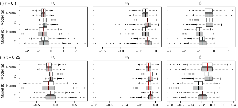
Figure 1: Box plots for the weighted estimator $\widehat{\theta}_{\tau n}$ (white boxes) and the unweighted estimator $\widecheck{\theta}_{\tau n}$ (grey boxes), at $\tau=0.1$ or 0.25, for two models with normally or Student’s $t_{5}$ distributed innovations. Model (a): $(\alpha_{0},\alpha_{1},\beta_{1})=(0.4,0.2,0.2)$; Model (b): $(\alpha_{0},\alpha_{1},\beta_{1})=(0.4,0.2,0.6)$. The thick black line in the center of the box indicates the sample median, and the thin red line indicates the value of the corresponding element of the true parameter vector $\theta_{\tau 0}$. The notations $\alpha_{0}$, $\alpha_{1}$ and $\beta_{1}$ represent the corresponding elements of $\widehat{\theta}_{\tau n}$ and $\widecheck{\theta}_{\tau n}$.

The first experiment compares the efficiency of the weighted quantile regression estimator $\widehat{\theta}_{\tau n}$ and its unweighted counterpart $\widecheck{\theta}_{\tau n}$. We generate the data from the GARCH($1,1$) model in (5.1) with standard normal or standardized Student’s $t_{5}$ distributed innovations $\{\eta_{t}\}$, using two sets of parameters: $(\alpha_{0},\alpha_{1},\beta_{1})=(0.4,0.2,0.2)$ (Model (a)) and $(\alpha_{0},\alpha_{1},\beta_{1})=(0.4,0.2,0.6)$ (Model (b)). These settings ensure strict stationarity of $\{x_{t}\}$ with $E|x_{t}|^{4+\iota_{0}}<\infty$ for some $\iota_{0}>0$, as required in Corollary 1; see Ling & McAleer (2002) for the existence of moments of GARCH models. Particularly, the available parameter space of $\alpha_{1}$ is severely restricted in the Student’s $t_{5}$ case. The sample size is $n=2000$, and two quantile levels, $\tau=0.1$ and 0.25, are considered. Figure 1 provides the box plots for the two estimators based on 1000 replications. It shows that the interquartile range of the weighted estimator $\widehat{\theta}_{\tau n}$ is smaller than that of the unweighted $\widecheck{\theta}_{\tau n}$ under all settings; the latter also suffers from more severe outliers. The efficiency gains from the weights seem larger for the Student’s $t_{5}$ cases. Moreover, for the unweighted estimator $\widecheck{\theta}_{\tau n}$, the sample median slightly deviates from the true value $\theta_{\tau 0}$ especially when the innovations are Student’s $t_{5}$ distributed. The results suggest that the weighted estimator is more efficient in finite samples.

The second experiment examines the finite-sample performance of the estimator $\widehat{\theta}_{\tau n}$ further, as well as that of the residual QACF $r_{k,\tau}$ and the bootstrapping approximations. The data are generated from the GARCH($1,1$) model in (5.1) with $(\alpha_{0},\alpha_{1},\beta_{1})=(0.4,0.4,0.4)$ and the same settings for the innovations. The sample sizes are $n=500$, $1000$ and $2000$, with $1000$ replications generated for each sample size. Three distributions for the random weights $\{\omega_{t}\}$ in the bootstrapping procedure are considered: the standard exponential distribution ($W_{1}$); the Rademacher distribution ($W_{2}$), which takes the values 0 or 2, each with probability 0.5 (Li et al. 2014); and Mammen’s two-point distribution ($W_{3}$), which takes the value $(-\sqrt{5}+3)/2$ with probability $(\sqrt{5}+1)/2\sqrt{5}$ and the value $(\sqrt{5}+3)/2$ with probability $1-(\sqrt{5}+1)/2\sqrt{5}$ (Mammen 1993). As in the previous experiment, we examine two quantile levels, $\tau=0.1$ and 0.25.

The biases, empirical standard deviations (ESDs) and asymptotic standard deviations (ASDs) for $\widehat{\theta}_{\tau n}$ are reported in Table 3, and those for the residual QACF $r_{k,\tau}$ at lags $k=2,4$ and 6 are given in Table 4. All ASDs are computed according to the proposed bootstrapping procedure. From both tables, we have the following results: (1) the biases are small, and the ESDs and ASDs are fairly close to each other as $n$ increases to 1000; (2) as $n$ increases, the biases and standard deviations decrease, and the ESDs get closer to the corresponding ASDs; (3) the choice of random weights have little influence on the bootstrapping approximations; (4) the performance of the bootstrapping approximations are similar for both quantile levels as $n$ increases to 1000.

The third experiment evaluates the empirical size and power of the proposed bootstrapping test statistic $Q(K)$. The data generating processes are

$$x_{t}=\sqrt{h_{t}}\eta_{t},\hskip 14.22636pth_{t}=0.4+0.2x_{t-1}^{2}+dx_{t-4}^{2}+0.2h_{t-1},$$

where $\{\eta_{t}\}$ follow the same distribution as in the previous experiment, and we consider departure $d=0$, 0.3 or 0.6. We conduct the estimation assuming a GARCH($1,1$) model; thus, $d=0$ corresponds to the size of the test, and $d\neq 0$ corresponds to the power. All other settings are preserved from the previous experiment.

Table 5 reports the rejection rates of $Q(K)$ at the maximum lag $K=6$. It shows a satisfactory performance of both the size and the power. The sizes are close to the nominal rate $5\%$ for $n$ as small as 500, and the powers increase as either $n$ or the departure $d$ increases. Interestingly, the powers at $\tau=0.1$ and 0.25 are close when $\{\eta_{t}\}$ are Gaussian, yet differ notably when they are Student’s $t_{5}$ distributed. Moreover, it is worth noting that when the lower quantile $\tau$ is smaller, the actual departure in the quantile regression, namely $|b_{\tau}d|$, increases, yet meanwhile the density $f(b_{\tau})$ decreases, i.e., there are fewer data points around $b_{\tau}$. Hence, the effect of $\tau$ on the power is mixed, and the simulation result suggests that the overall impact of $\tau$ varies with the innovation distribution. Lastly, the different random weights distributions perform similarly, as in the previous experiment.

6 Empirical Analysis

This section demonstrates the usefulness of the proposed approach through analyzing daily log returns of three stock market indices: the S&P 500 index, the Dow 30 index, and the Hang Seng Index (HSI). The data are from January 2, 2008 to June 30, 2016.

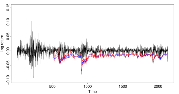
Figure 2: Time plot for daily log returns (black line) of S&P 500 from January 2, 2008 to June 30, 2016, with rolling forecasts of conditional quantiles (blue line) at $\tau=0.05$ from January 4, 2010 to June 30, 2016 and corresponding $95\%$ confidence bounds (red lines), using the proposed conditional quantile estimation and bootstrap method.

To begin with, we illustrate the estimation of the conditional quantiles of the daily log returns of the S&P 500 index. The sequence of log returns, denoted by $\{x_{t}\}$, has a sample size of 2139, and its time plot is shown in Figure 2. For the time being, we focus on $\tau=0.05$, which corresponds to the $5\%$ VaR. Throughout this section, the standard exponential random weights are used in the bootstrapping approximations.

We first consider an ARCH(1) model for $\{x_{t}\}$. The Gaussian QMLE gives following estimation result,

$$\widetilde{h}_{t}=2.608\times 10^{-7}_{6.222\times 10^{-6}}+0.864_{5.159}x_{t-1}^{2},$$ (6.1)

where the standard errors of the parameter estimates are written as the subscripts. Note that both the intercept and the ARCH coefficient are insignificant. We compute the initial estimates of $\{h_{t}\}$ by (6.1). Subsequently, using the proposed estimation method, we have that the fitted conditional quantile of $\{y_{t}\}$, with $y_{t}=T(x_{t})$, is

$$\widehat{Q}_{0.05}(y_{t}|\mathcal{F}_{t-1})=-2.717\times 10^{-4}_{7.554\times 10^{-5}}-1.659_{1.499}x_{t-1}^{2},$$

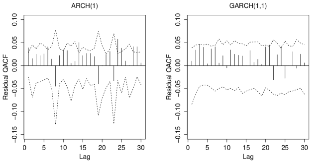
Figure 3: Residual QACFs for the fitted conditional quantiles at $\tau=0.05$, with corresponding 95% confidence bounds, for daily log returns of S&P 500.

where the coefficient of $x_{t-1}^{2}$ is insignificant, while the intercept is significant. We next check the adequacy of the fitted conditional quantile. The left panel of Figure 3 shows that the individual residual QACF exceeds the 95% confidence bounds at, e.g., lags 1, 6 and 14, by a relatively large margin. Moreover, the $p$-value of the bootstrapping test statistic $Q(K)$ with the maximum lag $K=6$ is as small as 0.039, and those of $Q(K)$ with $K=12$, 18, 24 and 30 are 0.228, 0.174, 0.127 and 0.088, respectively. The diagnostic tests indicate that there may be higher-order ARCH effects which are not captured by the fitted model.

In view of this, we next consider a GARCH($1,1$) model and estimate the conditional quantiles using the proposed estimation procedure. As a result, the initial estimates of $\{h_{t}\}$ are calculated from

$$\widetilde{h}_{t}=2.646\times 10^{-6}_{7.793\times 10^{-7}}+0.126_{0.018}x_{t-1}^{2}+0.858_{0.019}\widetilde{h}_{t-1},$$ (6.2)

and the fitted conditional quantile function is

$$\widehat{Q}_{0.05}(y_{t}|\mathcal{F}_{t-1})=-4.713\times 10^{-7}_{3.199\times 10^{-5}}-0.124_{0.261}x_{t-1}^{2}-3.007_{0.521}\widetilde{h}_{t-1}.$$ (6.3)

Interestingly, while all parameter estimates in (6.2) are significant, only the coefficient of $\widetilde{h}_{t-1}$ is significant in (6.3). Note that unlike the ARCH model, the conditional variances $\{h_{t}\}$ are defined recursively in the GARCH model. Therefore, the coefficient of $x_{t-1}^{2}$ in (6.2) incorporates ARCH effects of all orders, and its significance confirms that ARCH effects exist. That is, $h_{t}$ is not constant, even though the coefficient of $x_{t-1}^{2}$ in (6.1) is insignificant. On the contrary, the coefficient of $x_{t-1}^{2}$ in (6.3) contains only the effect of $x_{t-1}^{2}$ on the conditional quantile, as the higher order ARCH effects are already incorporated into the initial estimates $\widetilde{h}_{t-1}$. The insignificant coefficient of $x_{t-1}^{2}$ in (6.3) suggests that $x_{t-1}^{2}$ itself may have no contribution to the conditional quantile at $\tau=0.05$.

We next conduct diagnostic checking for the fitted conditional quantiles given by (6.3). As shown in the right panel of Figure 3, the residual QACF only slightly stands out of the 95% confidence bounds at lags 3, 21 and 24, and falls within them at all the other lags. Furthermore, the $p$-values of $Q(K)$ are always larger than 0.257 for $K=6$, 12, 18, 24 and 30, indicating the adequacy of the fitted conditional quantiles.

Moreover, to examine the forecasting performance of the proposed approach, we consider the rolling forecast of conditional quantiles at $\tau=0.05$, i.e., the negative 5% VaR over a one-day horizon. We first conduct the estimation for the first two years’ data (January 2, 2008 to December 31, 2009) under the GARCH($1,1$) model assumption, and compute the conditional quantile forecast for the next trading day, i.e., the forecast of $Q_{\tau}(x_{n+1}|\mathcal{F}_{n})$. Then we advance the forecasting origin by one, and, with one more observation included in the estimation subsample, repeat the foregoing procedure until we reach the end of the data set. For each rolling step, we use the proposed bootstrap method to construct the 95% confidence interval for the conditional quantile. The rolling forecasts and the corresponding confidence intervals are provided in Figure 2. It shows that $x_{t}$ falls below the conditional quantile forecast only occasionally, which supports the reliable performance of the proposed estimation and bootstrap method.

Finally, to better evaluate the forecasting performance of the proposed method, we conduct a more extensive analysis using the daily log returns of all the three stock market indices, and provide a comparison with the various conditional quantile estimation methods employed in the simulation experiment in Section 5.1. We examine two quantile levels: $\tau=0.05$ and 0.01, which correspond to the one-day 5% and 1% VaR. The foregoing rolling procedure is adopted, and forecasting performance is measured by the empirical coverage rate (ECR), namely the proportion of observations that fall below the corresponding conditional quantile forecasts. The sample sizes for the Dow 30 index and the HSI are 2139 and 2130 respectively.

Table 6 reports the ECRs for the whole forecasting period as well as those for four separate subperiods: (1) January 4, 2010 to December 30, 2011; (2) January 3, 2012 to December 31, 2013; (3) January 2, 2014 to December 31, 2015; and (4) January 4, 2016 to June 30, 2016. For the ECRs of the whole period, the proposed hybrid method always gives the ECR closest to the nominal rate among all methods, for both 1% and 5% VaR and all market indices, except the case of 1% VaR for the HSI. Although the results for the subperiods are more mixed, it seems that the hybrid method is still most likely to give the best ECR. Specifically, the number of times a method gives the best ECR (including ties) among all methods for any subperiod and any quantile level are: 16 for Hybrid, 4 for $\text{QGARCH}_{1}$, 7 for $\text{QGARCH}_{2}$, 6 for CAViaR, and 7 for RiskM. The forecasting performance therefore corroborates the usefulness of the proposed method.

7 Conclusion and Discussion

Although quantile regression by nature is highly relevant to the conditional quantile estimation for time series models with conditional heteroscedasticity, it has been a very challenging task for the most important member of this family, i.e., Bollerslev’s (1986) GARCH model. The major technical difficulties are due to the presence of latent variables and the square-root form of the conditional quantile function of this model. In this paper, we propose an easy-to-implement quantile regression method for this important model. Our approach rests upon a monotone transformation which directly links the conditional quantile of the GARCH model to that of the linear GARCH model whose structure is much more tractable. As a result, quantile regression estimation for the GARCH model is made easy. Meanwhile, the original GARCH form enables reliable initial estimation for the conditional variances via the Gaussian QMLE.

Inference about the conditional quantile is conducted, including construction of confidence intervals and diagnostic checks. To approximate the asymptotic distributions of the proposed estimator and statistics, we introduce a new bootstrap method, and through replacing an optimization step with a sample averaging, we speed up the bootstrapping procedure significantly. To sum up, a complete approach to the conditional quantile inference for the widely used GARCH model is provided in this paper.

The proposed approach can be extended in several directions. First, it is well known that financial time series can be so heavy-tailed that $E(\eta_{t}^{4})=\infty$ (Hall & Yao 2003, Mittnik & Paolella 2003, Mikosch & Stărică 2000). For such cases, we may alternatively consider methods that are more robust than the Gaussian QMLE for the initial estimation of the conditional variances, including the least absolute deviation estimator of Peng & Yao (2003) and the rank-based estimator of Andrews (2012) among others. Second, our approach can be applied to the conditional quantile estimation for other conditional heteroscedastic models, including the asymmetric GJR-GARCH model (Glosten et al. 1993). Third, although the multivariate GARCH model has been widely used for the volatility modeling of multiple asset returns (Engle & Kroner 1995), the conditional quantile estimation for the corresponding portfolio returns is still an open problem. The proposed hybrid conditional quantile inference procedure offers some preliminary ideas on this, and we will leave it for future research.

Appendix: Technical Details

This appendix gives the proofs of Theorems 1-4, Corollaries 1-3 and Equation (2.5). Lemmas A.1 and A.2 contain some preliminary results for GARCH models which will be repeatedly used later.

Throughout the appendix, $C$ is a generic positive constant which may take different values at its different occurrences, and $C(M)$ is such a constant whose value depends on $M$. We denote by $\|\cdot\|$ the norm of a matrix or column vector, defined as $\|A\|=\sqrt{\text{tr}(AA^{\prime})}=\sqrt{\sum_{i,j}|a_{ij}|^{2}}$. In addition, let $z_{t}(\theta)=(1,x_{t-1}^{2},\dots,x_{t-q}^{2},h_{t-1}(\theta),\dots,h_{t-p}(\theta))^{\prime}$, $\widetilde{z}_{t}(\theta)=(1,x_{t-1}^{2},\dots,x_{t-q}^{2},\widetilde{h}_{t-1}(\theta),\dots,\widetilde{h}_{t-p}(\theta))^{\prime}$, and, for simplicity, write $z_{t}=z_{t}(\theta_{0})$, $\breve{z}_{t}=\widetilde{z}_{t}(\theta_{0})$, and $\widetilde{z}_{t}=\widetilde{z}_{t}(\widetilde{\theta}_{n})$, where $\widetilde{\theta}_{n}$ is the Gaussian QMLE of model (1.1). In the proofs of Theorems 2 and 4, the notations $E^{*}$, $O_{p}^{*}(1)$ and $o_{p}^{*}(1)$ correspond to the bootstrapped probability space.

Lemma A.1.

Under Assumption 1, for any $\kappa>0$, there exists a constant $c>0$ such that

$$(i)\;E\left(\sup\left\{\frac{h_{t}(\theta_{2})}{h_{t}(\theta_{1})}:\|\theta_{1}-\theta_{2}\|\leq c,\;\theta_{1},\theta_{2}\in\Theta\right\}\right)^{\kappa}<\infty,$$

$$(ii)\;E\sup\left\{\left\|\frac{1}{h_{t}(\theta_{1})}\frac{\partial h_{t}(\theta_{2})}{\partial\theta}\right\|^{\kappa}:\|\theta_{1}-\theta_{2}\|\leq c,\;\theta_{1},\theta_{2}\in\Theta\right\}<\infty,$$

$$(iii)\;E\sup\left\{\left\|\frac{1}{h_{t}(\theta_{1})}\frac{\partial^{2}h_{t}(\theta_{2})}{\partial\theta\partial\theta^{\prime}}\right\|^{\kappa}:\|\theta_{1}-\theta_{2}\|\leq c,\;\theta_{1},\theta_{2}\in\Theta\right\}<\infty$$

and

$$(iv)\;E\sup\left\{\left|\frac{1}{h_{t}(\theta_{1})}\frac{\partial^{3}h_{t}(\theta_{2})}{\partial\theta_{i}\partial\theta_{k}\partial\theta_{\ell}}\right|^{\kappa}:\|\theta_{1}-\theta_{2}\|\leq c,\;\theta_{1},\theta_{2}\in\Theta\right\}<\infty,$$

for all $1\leq i,k,\ell\leq p+q+1$.

Proof of Lemma A.1.

We first prove (i). For any $\theta=(\alpha_{0},\alpha_{1},\dots,\alpha_{q},\beta_{1},\dots,\beta_{p})^{\prime}\in\Theta$ and $\gamma>1$, define

$$U(\gamma,\theta)=\{\theta^{*}=(\alpha_{0}^{*},\alpha_{1}^{*},\dots,\alpha_{q}^{*},\beta_{1}^{*},\dots,\beta_{p}^{*})^{\prime}\in\Theta:\max_{1\leq j\leq p}\frac{\beta_{j}^{*}}{\beta_{j}}\leq\gamma\}.$$

Claim (i) follows from a more general result: for any $\kappa>0$, there is $\gamma>1$ such that

$$E\left[\sup_{\theta\in\Theta}\sup_{\theta^{*}\in U(\gamma,\theta)}\frac{h_{t}(\theta^{*})}{h_{t}(\theta)}\right]^{\kappa}<\infty.$$ (A.1)

Notice that for any $\theta$, the set $U(\gamma,\theta)$ only imposes an upper bound on the $\beta_{j}^{*}$’s, while the condition $\|\theta_{1}-\theta_{2}\|\leq c$ restricts the distance between $\theta_{1}$ and $\theta_{2}$.

We shall prove (A.1). Note that the functions $h_{t}(\theta)$, as defined recursively in (2.2), can be written in the form of

$$h_{t}(\theta)=c_{0}(\theta)+\sum_{j=1}^{\infty}c_{j}(\theta)x_{t-j}^{2},$$

and the series converges with probability one for all $\theta\in\Theta$; see, e.g., Berkes et al. (2003). Moreover, $c_{0}(\theta)=\alpha_{0}/(1-\beta_{1}-\cdots-\beta_{p})\geq C_{1}=\underline{w}/(1-p\underline{w})>0$ for all $\theta\in\Theta$, and from Lemma 3.1 in Berkes et al. (2003), it holds that

$$\sup_{\theta\in\Theta}c_{j}(\theta)\leq C_{2}\rho_{1}^{j},\hskip 14.22636ptj\geq 0,$$ (A.2)

where $\rho_{1}=\rho_{0}^{1/p}\in(0,1)$, and

$$\sup_{\theta\in\Theta}\sup_{\theta^{*}\in U(\gamma,\theta)}\frac{c_{j}(\theta^{*})}{c_{j}(\theta)}\leq C_{3}\gamma^{j},\hskip 14.22636ptj\geq 0,$$ (A.3)

for some constants $C_{2},C_{3}>0$. Using (A.3), we have

$$\ \sup_{\theta\in\Theta}\sup_{\theta^{*}\in U(\gamma,\theta)}\frac{h_{t}(\theta^{*})}{h_{t}(\theta)}\leq\frac{C_{2}}{C_{1}}+C_{3}\sup_{\theta\in\Theta}\dfrac{\sum_{j=1}^{\infty}\gamma^{j}c_{j}(\theta)x_{t-j}^{2}}{C_{1}+\sum_{j=1}^{\infty}c_{j}(\theta)x_{t-j}^{2}},$$

and then it suffices to show that for any $\kappa\geq 1$,

$$\left\|\sup_{\theta\in\Theta}\dfrac{\sum_{j=1}^{\infty}\gamma^{j}c_{j}(\theta)x_{t-j}^{2}}{C_{1}+\sum_{j=1}^{\infty}c_{j}(\theta)x_{t-j}^{2}}\right\|_{\kappa}<\infty,$$

where $\|\cdot\|_{\kappa}$ denotes the $L_{\kappa}$ norm, i.e., $\|X\|_{\kappa}=(E|X|^{\kappa})^{1/\kappa}$. Note that there is $\delta_{0}>0$ such that $E|x_{0}^{2}|^{\delta_{0}}<\infty$. Thus, for any $\kappa\geq 1$ and $\delta_{1}\in(1-\delta_{0}/\kappa,1)$, by (A.2) and the Minkowski inequality, we have

$$\left\|\sup_{\theta\in\Theta}\dfrac{\sum_{j=1}^{\infty}\gamma^{j}c_{j}(\theta)x_{t-j}^{2}}{C_{1}+\sum_{j=1}^{\infty}c_{j}(\theta)x_{t-j}^{2}}\right\|_{\kappa} \leq\left\|\sup_{\theta\in\Theta}\sum_{j=1}^{\infty}\dfrac{\gamma^{j}c_{j}(\theta)x_{t-j}^{2}}{C_{1}^{1-{\delta_{1}}}[c_{j}(\theta)x_{t-j}^{2}]^{{\delta_{1}}}}\right\|_{\kappa}$$

$$\leq C_{1}^{-(1-{\delta_{1}})}\left\|\sum_{j=1}^{\infty}\gamma^{j}(C_{2}\rho_{1}^{j}x_{t-j}^{2})^{1-{\delta_{1}}}\right\|_{\kappa}$$

$$\leq C\sum_{j=1}^{\infty}(\gamma\rho_{1}^{1-{\delta_{1}}})^{j}\left[E|x_{0}^{2}|^{(1-{\delta_{1}})\kappa}\right]^{1/\kappa}<\infty,$$

if $\gamma$ is close enough to 1. Therefore, (A.1) holds, and so does (i).

From the proof of Theorem 2.2 in Francq & Zakoian (2004), under Assumption 1, for any $\kappa>0$,

$$E\sup_{\theta\in\Theta}\left\|\frac{1}{h_{t}(\theta)}\frac{\partial h_{t}(\theta)}{\partial\theta}\right\|^{\kappa}<\infty,\hskip 14.22636ptE\sup_{\theta\in\Theta}\left\|\frac{1}{h_{t}(\theta)}\frac{\partial^{2}h_{t}(\theta)}{\partial\theta\partial\theta^{\prime}}\right\|^{\kappa}<\infty\hskip 14.22636pt\text{and}\hskip 14.22636pt$$

$$E\sup_{\theta\in\Theta}\left|\frac{1}{h_{t}(\theta)}\frac{\partial^{3}h_{t}(\theta)}{\partial\theta_{i}\partial\theta_{k}\partial\theta_{\ell}}\right|^{\kappa}<\infty,$$

where $1\leq i,k,\ell\leq p+q+1$; see also Lemma 3.6 in Berkes & Horváth (2004). Combining these with (i), we immediately obtain (ii)-(iv).    

Lemma A.2.

Under Assumption 1,

$$\sup_{\theta\in\Theta}|\widetilde{h}_{t}(\theta)-h_{t}(\theta)|\leq C\rho^{t}\zeta\hskip 14.22636pt\text{and}\hskip 14.22636pt\sup_{\theta\in\Theta}\left\|\frac{\partial\widetilde{h}_{t}(\theta)}{\partial\theta}-\frac{\partial h_{t}(\theta)}{\partial\theta}\right\|\leq C\rho^{t}\zeta,$$

where $C>0$ and $0<\rho<1$ are constants, and $\zeta$ is a random variable independent of $t$ with $E|\zeta|^{\delta_{0}}<\infty$ for some $\delta_{0}>0$.

Proof of Lemma A.2.

The lemma can be proved by a method similar to that for Equations (6) and (7) in the proof of Theorem 1 in Zheng et al. (2016).    

Proof of Theorem 1.

Let $L_{n}(\theta)=\sum_{t=1}^{n}\widetilde{h}_{t}^{-1}\rho_{\tau}(y_{t}-\theta^{\prime}\widetilde{z}_{t})$ and $\breve{L}_{n}(\theta)=\sum_{t=1}^{n}\widetilde{h}_{t}^{-1}\rho_{\tau}(y_{t}-\theta^{\prime}\breve{z}_{t})$. Notice that for $x\neq 0$,

$$\rho_{\tau}(x-y)-\rho_{\tau}(x)=-y\psi_{\tau}(x)+\int_{0}^{y}[I(x\leq s)-I(x\leq 0)]ds,$$ (A.4)

where $\psi_{\tau}(x)=\tau-I(x<0)$; see Knight (1998). Then, for any fixed $u\in\mathbb{R}^{p+q+1}$,

$$L_{n}(\theta_{\tau 0}+n^{-1/2}u)-\breve{L}_{n}(\theta_{\tau 0})=-L_{1n}(u)+L_{2n}(u),$$ (A.5)

where

$$L_{1n}(u) =\sum_{t=1}^{n}\psi_{\tau}(\breve{e}_{t,\tau})\widetilde{h}^{-1}_{t}\left[(\theta_{\tau 0}+n^{-1/2}u)^{\prime}\widetilde{z}_{t}-\theta_{\tau 0}^{\prime}\breve{z}_{t}\right],$$

$$L_{2n}(u) =\sum_{t=1}^{n}\widetilde{h}^{-1}_{t}\int_{0}^{(\theta_{\tau 0}+n^{-1/2}u)^{\prime}\widetilde{z}_{t}-\theta_{\tau 0}^{\prime}\breve{z}_{t}}\left[I(\breve{e}_{t,\tau}\leq s)-I(\breve{e}_{t,\tau}\leq 0)\right]ds,$$

and $\breve{e}_{t,\tau}=y_{t}-\theta_{\tau 0}^{\prime}\breve{z}_{t}$. Let $u^{(j)}$ be the $(j+q+1)$-th element of $u$, and denote $\beta_{\tau 0}^{(j)}=b_{\tau}\beta_{0j}$, for $j=1,\dots,p$. It can be verified that

$$(\theta_{\tau 0}+n^{-1/2}u)^{\prime}\widetilde{z}_{t}-\theta_{\tau 0}^{\prime}\breve{z}_{t}=\xi_{1nt}(\widetilde{\theta}_{n})+\xi_{2nt}(\widetilde{\theta}_{n})+\xi_{3nt}(\widetilde{\theta}_{n}),$$ (A.6)

where

$$\begin{split}\xi_{1nt}(\theta)&=n^{-1/2}u^{\prime}z_{t}+\sum_{j=1}^{p}\beta_{\tau 0}^{(j)}\frac{\partial h_{t-j}(\theta_{0})}{\partial\theta^{\prime}}(\theta-\theta_{0}),\\ \xi_{2nt}(\theta)&=\frac{1}{\sqrt{n}}\sum_{j=1}^{p}u^{(j)}[h_{t-j}(\theta)-h_{t-j}]+\sum_{j=1}^{p}\beta_{\tau 0}^{(j)}\bigg{[}h_{t-j}(\theta)-h_{t-j}-\frac{\partial h_{t-j}(\theta_{0})}{\partial\theta^{\prime}}(\theta-\theta_{0})\bigg{]},\\ \xi_{3nt}(\theta)&=\frac{1}{\sqrt{n}}\sum_{j=1}^{p}u^{(j)}[\widetilde{h}_{t-j}(\theta)-h_{t-j}(\theta)]\\ &\hskip 14.22636pt+\sum_{j=1}^{p}\beta_{\tau 0}^{(j)}\left\{[\widetilde{h}_{t-j}(\theta)-h_{t-j}(\theta)]-[\widetilde{h}_{t-j}(\theta_{0})-h_{t-j}]\right\}.\end{split}$$

For any $M>0$, denote $\Theta_{n}=\Theta_{n}(M)=\{\theta\in\Theta:\|\theta-\theta_{0}\|\leq n^{-1/2}M\}$. Using the Taylor expansion, it holds that

$$\sup_{\theta\in\Theta_{n}}|\xi_{2nt}(\theta)|\leq\frac{M}{n}\sum_{j=1}^{p}|u^{(j)}|\sup_{\theta\in\Theta_{n}}\left\|\frac{\partial h_{t-j}(\theta)}{\partial\theta}\right\|+\frac{M^{2}}{2n}\sum_{j=1}^{p}|\beta_{\tau 0}^{(j)}|\sup_{\theta\in\Theta_{n}}\left\|\frac{\partial^{2}h_{t-j}(\theta)}{\partial\theta\partial\theta^{\prime}}\right\|,$$ (A.7)

and by Lemma A.2,

$$\begin{split}&\sup_{\theta\in\Theta_{n}}|\xi_{3nt}(\theta)|\\ &\hskip 14.22636pt\leq\frac{1}{\sqrt{n}}\sum_{j=1}^{p}\bigg{[}|u^{(j)}|\sup_{\theta\in\Theta}|\widetilde{h}_{t-j}(\theta)-h_{t-j}(\theta)|+M|\beta_{\tau 0}^{(j)}|\sup_{\theta\in\Theta}\left\|\frac{\partial\widetilde{h}_{t-j}(\theta)}{\partial\theta}-\frac{\partial h_{t-j}(\theta)}{\partial\theta}\right\|\bigg{]}\\ &\hskip 14.22636pt\leq n^{-1/2}C(M)\rho^{t}\zeta.\end{split}$$ (A.8)

Moreover,

$$\breve{e}_{t,\tau}=(\varepsilon_{t}-b_{\tau})h_{t}+a_{t},\hskip 14.22636pt\text{where}\hskip 14.22636pta_{t}=\sum_{j=1}^{p}\beta_{\tau 0}^{(j)}[h_{t-j}-\widetilde{h}_{t-j}(\theta_{0})]\in\mathcal{F}_{0}.$$ (A.9)

We first consider $L_{1n}(u)$, which can be decomposed into four parts,

$$L_{1n}(u)=\sum_{t=1}^{n}A_{1nt}(\widetilde{\theta}_{n})+\sum_{t=1}^{n}A_{2nt}(\widetilde{\theta}_{n})+\sum_{t=1}^{n}A_{3nt}(\widetilde{\theta}_{n})+\sum_{t=1}^{n}A_{4nt}(\widetilde{\theta}_{n}),$$ (A.10)

where

$$A_{1nt}(\theta)=\psi_{\tau}(\breve{e}_{t,\tau})\widetilde{h}_{t}^{-1}(\theta)\xi_{3nt}(\theta)+\psi_{\tau}(\breve{e}_{t,\tau})[\widetilde{h}_{t}^{-1}(\theta)-h_{t}^{-1}(\theta)][\xi_{1nt}(\theta)+\xi_{2nt}(\theta)],$$

$$A_{2nt}(\theta)=[\psi_{\tau}(\breve{e}_{t,\tau})-\psi_{\tau}(\varepsilon_{t}-b_{\tau})]h_{t}^{-1}(\theta)[\xi_{1nt}(\theta)+\xi_{2nt}(\theta)],$$

$$A_{3nt}(\theta)=\psi_{\tau}(\varepsilon_{t}-b_{\tau})h_{t}^{-1}(\theta)\xi_{2nt}(\theta),\hskip 14.22636pt\text{and}\hskip 14.22636ptA_{4nt}(\theta)=\psi_{\tau}(\varepsilon_{t}-b_{\tau})h_{t}^{-1}(\theta)\xi_{1nt}(\theta).$$

Note that $\inf_{\theta\in\Theta}h_{t}(\theta)\geq\underline{w}$ and $\inf_{\theta\in\Theta}\widetilde{h}_{t}(\theta)\geq\underline{w}$. By Lemma A.2, (A.7) and (LABEL:beq12), we can show that

$$\begin{split}\sup_{\theta\in\Theta_{n}}\left|\sum_{t=1}^{n}A_{1nt}(\theta)\right|&\leq\frac{1}{\underline{w}}\sum_{t=1}^{n}\sup_{\theta\in\Theta_{n}}|\xi_{3nt}(\theta)|+\frac{C\zeta}{\underline{w}^{2}}\sum_{t=1}^{n}\rho^{t}\sup_{\theta\in\Theta_{n}}(|\xi_{1nt}(\theta)|+|\xi_{2nt}(\theta)|)\\ &=o_{p}(1),\end{split}$$ (A.11)

which, together with the fact that $\sqrt{n}(\widetilde{\theta}_{n}-\theta_{0})=O_{p}(1)$, implies that

$$\sum_{t=1}^{n}A_{1nt}(\widetilde{\theta}_{n})=o_{p}(1).$$ (A.12)

Note that by Lemma A.2 and Assumption 2, we have

$$|F(b_{\tau})-F(b_{\tau}-h_{t}^{-1}a_{t})|\leq\sup_{x\in\mathbb{R}}f(x)\sum_{j=1}^{p}\frac{|\beta_{\tau 0}^{(j)}|}{\underline{w}}|h_{t-j}(\theta_{0})-\widetilde{h}_{t-j}(\theta_{0})|\leq C\rho^{t}\zeta.$$

It then follows from (A.9) that

$$E|\psi_{\tau}(\breve{e}_{t,\tau})-\psi_{\tau}(\varepsilon_{t}-b_{\tau})| =E|F(b_{\tau})-F(b_{\tau}-h_{t}^{-1}a_{t})|$$

$$=E[|F(b_{\tau})-F(b_{\tau}-h_{t}^{-1}a_{t})|I(C\rho^{t}\zeta\leq\rho^{t/2})]$$

$$\hskip 14.22636pt+E[|F(b_{\tau})-F(b_{\tau}-h_{t}^{-1}a_{t})|I(C\rho^{t}\zeta>\rho^{t/2})]$$

$$\leq\rho^{t/2}+\mathrm{Pr}(C\rho^{t}\zeta>\rho^{t/2})\leq\rho^{t/2}+C\rho^{{\delta_{0}}t/2},$$ (A.13)

where we used the Markov inequality and the fact that $E|\zeta|^{\delta_{0}}<\infty$. Moreover,

$$\|h^{-1}_{t}z_{t}\|\leq\frac{\sqrt{p+q+1}}{\underline{w}},$$ (A.14)

$$\sup_{\theta_{1},\theta_{2}\in\Theta_{n}}\left|\frac{\xi_{1nt}(\theta_{2})}{h_{t}(\theta_{1})}\right|\leq\frac{|h_{t}^{-1}u^{\prime}z_{t}|}{\sqrt{n}}\sup_{\theta\in\Theta_{n}}\frac{h_{t}}{h_{t}(\theta)}+\frac{M}{\underline{w}\sqrt{n}}\sum_{j=1}^{p}|\beta_{\tau 0}^{(j)}|\sup_{\theta\in\Theta_{n}}\left\|\frac{1}{h_{t-j}(\theta)}\frac{\partial h_{t-j}(\theta_{0})}{\partial\theta}\right\|,$$ (A.15)

and by the Taylor expansion,

$$\begin{split}\sup_{\theta_{1},\theta_{2}\in\Theta_{n}}\left|\frac{\xi_{2nt}(\theta_{2})}{h_{t}(\theta_{1})}\right|&\leq\frac{M}{\underline{w}n}\sum_{j=1}^{p}|u^{(j)}|\sup_{\theta_{1},\theta_{2}\in\Theta_{n}}\left\|\frac{1}{h_{t-j}(\theta_{1})}\frac{\partial h_{t-j}(\theta_{2})}{\partial\theta}\right\|\\ &\hskip 14.22636pt+\frac{M^{2}}{2\underline{w}n}\sum_{j=1}^{p}|\beta_{\tau 0}^{(j)}|\sup_{\theta_{1},\theta_{2}\in\Theta_{n}}\left\|\frac{1}{h_{t-j}(\theta_{1})}\frac{\partial^{2}h_{t-j}(\theta_{2})}{\partial\theta\partial\theta^{\prime}}\right\|.\end{split}$$ (A.16)

As a result, by the Hölder inequality, Lemma A.1 and (Proof of Theorem 1.)-(A.16), we have

$$\begin{split}E\sup_{\theta\in\Theta_{n}}\left|\sum_{t=1}^{n}A_{2nt}(\theta)\right|&\leq\sum_{t=1}^{n}\left[E|\psi_{\tau}(\breve{e}_{t,\tau})-\psi_{\tau}(\varepsilon_{t}-b_{\tau})|\right]^{1/2}\left[E\sup_{\theta\in\Theta_{n}}\left(\frac{|\xi_{1nt}(\theta)|+|\xi_{2nt}(\theta)|}{h_{t}(\theta)}\right)^{2}\right]^{1/2}\\ &=o(1),\end{split}$$

which, together with the fact that $\sqrt{n}(\widetilde{\theta}_{n}-\theta_{0})=O_{p}(1)$, implies that

$$\sum_{t=1}^{n}A_{2nt}(\widetilde{\theta}_{n})=o_{p}(1).$$ (A.17)

Applying the Taylor expansion to $h^{-1}_{t}(\theta)$ and $\xi_{2nt}(\theta)$ respectively, we have

$$h_{t}^{-1}(\theta)\xi_{2nt}(\theta)=\xi_{4nt}(\theta)+\xi_{5nt}(\theta),$$ (A.18)

where

$$\xi_{4nt}(\theta) =\frac{1}{\sqrt{n}}\sum_{j=1}^{p}\frac{u^{(j)}}{h_{t}}\frac{\partial h_{t-j}(\theta_{0})}{\partial\theta^{\prime}}(\theta-\theta_{0})+\dfrac{1}{2}(\theta-\theta_{0})^{\prime}\sum_{j=1}^{p}\frac{\beta_{\tau 0}^{(j)}}{h_{t}}\frac{\partial^{2}h_{t-j}(\theta_{0})}{\partial\theta\partial\theta^{\prime}}(\theta-\theta_{0}),$$

$$\xi_{5nt}(\theta) =-\frac{\xi_{2nt}(\theta)}{h_{t}^{2}(\theta^{*}_{1})}\frac{\partial h_{t}(\theta^{*}_{1})}{\partial\theta^{\prime}}(\theta-\theta_{0})+\frac{(\theta-\theta_{0})^{\prime}}{2\sqrt{n}}\sum_{j=1}^{p}\frac{u^{(j)}}{h_{t}}\frac{\partial^{2}h_{t-j}(\theta^{*}_{2})}{\partial\theta\partial\theta^{\prime}}(\theta-\theta_{0})$$

$$\hskip 14.22636pt+\dfrac{1}{6}\sum_{j=1}^{p}\sum_{i,k,\ell=1}^{p+q+1}\frac{\beta_{\tau 0}^{(j)}}{h_{t}}\frac{\partial^{3}h_{t-j}(\theta^{*}_{2})}{\partial\theta_{i}\partial\theta_{k}\partial\theta_{\ell}}(\theta_{i}-\theta_{0i})(\theta_{k}-\theta_{0k})(\theta_{\ell}-\theta_{0\ell}),$$

with $\theta_{1}^{*}$ and $\theta_{2}^{*}$ both between $\theta$ and $\theta_{0}$. Then, it follows from Lemma A.1, the ergodic theorem and $\sqrt{n}(\widetilde{\theta}_{n}-\theta_{0})=O_{p}(1)$ that

$$\sum_{t=1}^{n}\psi_{\tau}(\varepsilon_{t}-b_{\tau})\xi_{4nt}(\widetilde{\theta}_{n})=o_{p}(1)$$ (A.19)

and

$$E\sup_{\theta\in\Theta_{n}}\left|\sum_{t=1}^{n}\psi_{\tau}(\varepsilon_{t}-b_{\tau})\xi_{5nt}(\theta)\right|\leq\sum_{t=1}^{n}E\sup_{\theta\in\Theta_{n}}|\xi_{5nt}(\theta)|=O(n^{-1/2}),$$ (A.20)

which implies

$$\sum_{t=1}^{n}A_{3nt}(\widetilde{\theta}_{n})=o_{p}(1).$$ (A.21)

By a method similar to that for $\sum_{t=1}^{n}A_{3nt}(\widetilde{\theta}_{n})$, we can show that

$$\sum_{t=1}^{n}\psi_{\tau}(\varepsilon_{t}-b_{\tau})[h_{t}^{-1}(\widetilde{\theta}_{n})-h_{t}^{-1}]\xi_{1nt}(\widetilde{\theta}_{n})=o_{p}(1),$$

which implies

$$\sum_{t=1}^{n}A_{4nt}(\widetilde{\theta}_{n}) =\sum_{t=1}^{n}\psi_{\tau}(\varepsilon_{t}-b_{\tau})h_{t}^{-1}\xi_{1nt}(\widetilde{\theta}_{n})+o_{p}(1)=u^{\prime}T_{1n}+T_{2n}+o_{p}(1),$$ (A.22)

where

$$T_{1n}=\frac{1}{\sqrt{n}}\sum_{t=1}^{n}\psi_{\tau}(\varepsilon_{t}-b_{\tau})\frac{z_{t}}{h_{t}}\hskip 5.69054pt\text{and}\hskip 5.69054ptT_{2n}=\sqrt{n}(\widetilde{\theta}_{n}-\theta_{0})^{\prime}\frac{1}{\sqrt{n}}\sum_{t=1}^{n}\psi_{\tau}(\varepsilon_{t}-b_{\tau})\sum_{j=1}^{p}\frac{\beta_{\tau 0}^{(j)}}{h_{t}}\frac{\partial h_{t-j}(\theta_{0})}{\partial\theta}.$$

Combining (A.10), (A.12), (A.17), (A.21), and (A.22), we have

$$L_{1n}(u)=u^{\prime}T_{1n}+T_{2n}+o_{p}(1).$$ (A.23)

Next we consider $L_{2n}(u)$. For simplicity, denote $I_{t}^{*}(s)=I(\breve{e}_{t,\tau}\leq s)-I(\breve{e}_{t,\tau}\leq 0)$. From (A.6), we have the decomposition

$$L_{2n}(u)=\sum_{t=1}^{n}B_{1nt}(\widetilde{\theta}_{n})+\sum_{t=1}^{n}B_{2nt}(\widetilde{\theta}_{n})+\sum_{t=1}^{n}B_{3nt}(\widetilde{\theta}_{n})+\sum_{t=1}^{n}B_{4nt}(\widetilde{\theta}_{n}),$$ (A.24)

where

$$B_{1nt}(\theta) =\widetilde{h}_{t}^{-1}(\theta)\int_{\xi_{1nt}(\theta)+\xi_{2nt}(\theta)}^{\xi_{1nt}(\theta)+\xi_{2nt}(\theta)+\xi_{3nt}(\theta)}I_{t}^{*}(s)ds+[\widetilde{h}^{-1}_{t}(\theta)-h^{-1}_{t}(\theta)]\int_{0}^{\xi_{1nt}(\theta)+\xi_{2nt}(\theta)}I_{t}^{*}(s)ds,$$

$$B_{2nt}(\theta) =h^{-1}_{t}(\theta)\int_{\xi_{1nt}(\theta)}^{\xi_{1nt}(\theta)+\xi_{2nt}(\theta)}I_{t}^{*}(s)ds,$$

$$B_{3nt}(\theta) =[h^{-1}_{t}(\theta)-h^{-1}_{t}]\int_{0}^{\xi_{1nt}(\theta)}I_{t}^{*}(s)ds,\hskip 14.22636pt\text{and}\hskip 14.22636ptB_{4nt}(\theta)=h^{-1}_{t}\int_{0}^{\xi_{1nt}(\theta)}I_{t}^{*}(s)ds.$$

By a method similar to that for (A.12), we can show that

$$\begin{split}\sup_{\theta\in\Theta_{n}}\left|\sum_{t=1}^{n}B_{1nt}(\theta)\right|&\leq\sum_{t=1}^{n}\sup_{\theta\in\Theta_{n}}\left[\frac{|\xi_{3nt}(\theta)|}{\widetilde{h}_{t}(\theta)}+\left|\frac{1}{\widetilde{h}_{t}(\theta)}-\frac{1}{h_{t}(\theta)}\right|\left(|\xi_{1nt}(\theta)|+|\xi_{2nt}(\theta)|\right)\right]\\ &=o_{p}(1),\end{split}$$ (A.25)

which, together with the fact that $\sqrt{n}(\widetilde{\theta}_{n}-\theta_{0})=O_{p}(1)$, implies

$$\sum_{t=1}^{n}B_{1nt}(\widetilde{\theta}_{n})=o_{p}(1).$$ (A.26)

From (A.9), (A.15), (A.16), Assumption 2 and the Hölder inequality, we have

$$E\sup_{\theta\in\Theta_{n}}\left|\sum_{t=1}^{n}B_{2nt}(\theta)\right|$$

$$\hskip 14.22636pt\leq E\sum_{t=1}^{n}\sup_{\theta\in\Theta_{n}}|h^{-1}_{t}(\theta)\xi_{2nt}(\theta)|I\left(|\breve{e}_{t,\tau}|\leq\sup_{\theta\in\Theta_{n}}\left(|\xi_{1nt}(\theta)|+|\xi_{2nt}(\theta)|\right)\right)$$

$$\hskip 14.22636pt\leq\sqrt{2\sup_{x\in\mathbb{R}}f(x)}\sum_{t=1}^{n}\left[E\sup_{\theta\in\Theta_{n}}\left|\frac{\xi_{2nt}(\theta)}{h_{t}(\theta)}\right|^{2}\right]^{1/2}\left[E\sup_{\theta\in\Theta_{n}}\frac{\left(|\xi_{1nt}(\theta)|+|\xi_{2nt}(\theta)|\right)}{h_{t}}\right]^{1/2}$$

$$\hskip 14.22636pt=o(1),$$

which, combined with the fact that $\sqrt{n}(\widetilde{\theta}_{n}-\theta_{0})=O_{p}(1)$, yields

$$\sum_{t=1}^{n}B_{2nt}(\widetilde{\theta}_{n})=o_{p}(1).$$ (A.27)

Similarly, it follows from (A.9), (A.15), Assumption 2 and the Hölder inequality that

$$E\sup_{\theta\in\Theta_{n}}\left|\sum_{t=1}^{n}B_{3nt}(\theta)\right|\leq E\sum_{t=1}^{n}\sup_{\theta\in\Theta_{n}}\left|[h^{-1}_{t}(\theta)-h_{t}^{-1}]\xi_{1nt}(\theta)\right|I\left(|\breve{e}_{t,\tau}|\leq\sup_{\theta\in\Theta_{n}}|\xi_{1nt}(\theta)|\right)=o(1),$$

and then

$$\sum_{t=1}^{n}B_{3nt}(\widetilde{\theta}_{n})=o_{p}(1).$$ (A.28)

Finally, for $\sum_{t=1}^{n}B_{4nt}(\widetilde{\theta}_{n})$, denote

$$B_{4nt}^{*}(\theta)=h_{t}^{-1}\int_{0}^{\xi_{1nt}(\theta)}\left[F(b_{\tau}-h_{t}^{-1}a_{t}+h_{t}^{-1}s)-F(b_{\tau}-h_{t}^{-1}a_{t})\right]ds,$$

and we first show that

$$\sum_{t=1}^{n}B_{4nt}(\widetilde{\theta}_{n})=\sum_{t=1}^{n}B_{4nt}^{*}(\widetilde{\theta}_{n})+o_{p}(1).$$ (A.29)

For any $v\in\mathbb{R}^{p+q+1}$, let $\eta_{t}(v)=h_{t}^{-1}\int_{0}^{\xi_{1nt}(\theta_{0}+n^{-1/2}v)}I_{t}^{*}(s)ds$, and denote

$$S_{n}(v)=\sum_{t=1}^{n}\left[B_{4nt}(\theta_{0}+n^{-1/2}v)-B_{4nt}^{*}(\theta_{0}+n^{-1/2}v)\right]=\sum_{t=1}^{n}\left\{\eta_{t}(v)-E[\eta_{t}(v)|\mathcal{F}_{t-1}]\right\}.$$

For any fixed $v$ such that $\|v\|\leq M$, by (A.15), Lemma A.1 and Assumption 2, we have

$$E\eta_{t}^{2}(v) \leq E\left\{\frac{|\xi_{1nt}(\theta_{0}+n^{-1/2}v)|}{h_{t}^{2}}\int_{0}^{\xi_{1nt}(\theta_{0}+n^{-1/2}v)}[F(b_{\tau}-\frac{a_{t}}{h_{t}}+\frac{s}{h_{t}})-F(b_{\tau}-\frac{a_{t}}{h_{t}})]ds\right\}$$

$$\leq\dfrac{1}{2}\sup_{x\in\mathbb{R}}f(x)E|h_{t}^{-1}\xi_{1nt}(\theta_{0}+n^{-1/2}v)|^{3}\leq n^{-3/2}C,$$ (A.30)

implying that

$$ES_{n}^{2}(v)\leq\sum_{t=1}^{n}E\eta_{t}^{2}(v)=o(1).$$ (A.31)

Note that

$$h_{t}^{-1}\sup_{\|v_{1}-v_{2}\|\leq\delta}|\xi_{1nt}(\theta_{0}+n^{-1/2}v_{1})-\xi_{1nt}(\theta_{0}+n^{-1/2}v_{2})|\leq\frac{\delta}{\underline{w}\sqrt{n}}\sum_{j=1}^{p}|\beta_{\tau 0}^{(j)}|\left\|\frac{1}{h_{t-j}}\frac{\partial h_{t-j}(\theta_{0})}{\partial\theta}\right\|.$$

Then, for any $v_{1},v_{2}\in\mathbb{R}^{p+q+1}$ such that $\|v_{1}\|,\|v_{2}\|\leq M$, in view of (A.9), (A.15), Lemma A.1 and Assumption 2, we have

$$E\sup_{\|v_{1}-v_{2}\|\leq\delta}|\eta_{t}(v_{1})-\eta_{t}(v_{2})|$$

$$\hskip 14.22636pt=E\left[h_{t}^{-1}\sup_{\|v_{1}-v_{2}\|\leq\delta}\left|\int_{\xi_{1nt}(\theta_{0}+n^{-1/2}v_{2})}^{\xi_{1nt}(\theta_{0}+n^{-1/2}v_{1})}I_{t}^{*}(s)ds\right|\right]$$

$$\hskip 14.22636pt\leq E\bigg{[}h_{t}^{-1}\sup_{\|v_{1}-v_{2}\|\leq\delta}|\xi_{1nt}(\theta_{0}+n^{-1/2}v_{1})-\xi_{1nt}(\theta_{0}+n^{-1/2}v_{2})|I\big{(}|\breve{e}_{t,\tau}|\leq\sup_{\theta\in\Theta_{n}}|\xi_{1nt}(\theta)|\big{)}\bigg{]}$$

$$\hskip 14.22636pt\leq\frac{2\delta}{\underline{w}\sqrt{n}}\sup_{x\in\mathbb{R}}f(x)E\left(\sup_{\theta\in\Theta_{n}}\frac{|\xi_{1nt}(\theta)|}{h_{t}}\sum_{j=1}^{p}|\beta_{\tau 0}^{(j)}|\left\|\frac{1}{h_{t-j}}\frac{\partial h_{t-j}(\theta_{0})}{\partial\theta}\right\|\right)\leq n^{-1}\delta C,$$

and hence

$$E\sup_{\|v_{1}-v_{2}\|\leq\delta}|S_{n}(v_{1})-S_{n}(v_{2})|\leq 2\sum_{t=1}^{n}E\sup_{\|v_{1}-v_{2}\|\leq\delta}|\eta_{t}(v_{1})-\eta_{t}(v_{2})|\leq 2\delta C,$$

which, together with (A.31) and the finite covering theorem, implies $\sup_{\|v\|\leq M}|S_{n}(v)|=o_{p}(1)$, and then (A.29) holds.

By elementary calculation and the Taylor expansion, we have

$$\sum_{t=1}^{n}B_{4nt}^{*}(\theta) =\sum_{t=1}^{n}h_{t}^{-1}\int_{0}^{\xi_{1nt}(\theta)}f(b_{\tau}-h_{t}^{-1}a_{t})h_{t}^{-1}sds+R_{1n}(\theta)$$

$$=\frac{1}{2}f(b_{\tau})\sum_{t=1}^{n}h_{t}^{-2}\xi_{1nt}^{2}(\theta)+R_{2n}(\theta)+R_{1n}(\theta),$$ (A.32)

where

$$R_{1n}(\theta)=\frac{1}{2}\sum_{t=1}^{n}h_{t}^{-3}\int_{0}^{\xi_{1nt}(\theta)}\dot{f}(b_{\tau,t}^{*}(s))s^{2}ds,$$

with $b_{\tau,t}^{*}(s)$ lying between $b_{\tau}-h_{t}^{-1}a_{t}$ and $b_{\tau}-h_{t}^{-1}a_{t}+h_{t}^{-1}s$, and

$$R_{2n}(\theta)=\frac{1}{2}\sum_{t=1}^{n}h_{t}^{-2}\xi_{1nt}^{2}(\theta)[f(b_{\tau}-h_{t}^{-1}a_{t})-f(b_{\tau})].$$

Note that

$$\sup_{\theta\in\Theta_{n}}|R_{1n}(\theta)|\leq\frac{1}{6}\sup_{x\in\mathbb{R}}|\dot{f}(x)|\sum_{t=1}^{n}\sup_{\theta\in\Theta_{n}}\left|\frac{\xi_{1nt}(\theta)}{h_{t}}\right|^{3},$$

and by Lemma A.2,

$$\sup_{\theta\in\Theta_{n}}|R_{2n}(\theta)|\leq\frac{1}{2}C\sup_{x\in\mathbb{R}}|\dot{f}(x)|\zeta\sum_{t=1}^{n}\rho^{t}\sup_{\theta\in\Theta_{n}}\left|\frac{\xi_{1nt}(\theta)}{h_{t}}\right|^{2}.$$

Then, by (A.15), Lemma A.1 and Assumption 2, we have

$$R_{1n}(\widetilde{\theta}_{n})=o_{p}(1)\hskip 14.22636pt\text{and}\hskip 14.22636ptR_{2n}(\widetilde{\theta}_{n})=o_{p}(1).$$

Hence, by (A.24), (A.26)-(A.29) and (Proof of Theorem 1.), together with the ergodic theorem, we have

$$\begin{split}L_{2n}(u)&=\frac{1}{2}f(b_{\tau})\sum_{t=1}^{n}h_{t}^{-2}\xi_{1nt}^{2}(\widetilde{\theta}_{n})+o_{p}(1)\\ &=\frac{1}{2}f(b_{\tau})u^{\prime}\Omega_{2}u+b_{\tau}f(b_{\tau})u^{\prime}\Gamma_{2}\sqrt{n}(\widetilde{\theta}_{n}-\theta_{0})+T_{3n}+o_{p}(1),\end{split}$$ (A.33)

where

$$T_{3n}=\dfrac{1}{2}f(b_{\tau})(\widetilde{\theta}_{n}-\theta_{0})^{\prime}\sum_{t=1}^{n}\sum_{j_{1}=1}^{p}\sum_{j_{2}=1}^{p}\beta_{\tau 0}^{(j_{1})}\beta_{\tau 0}^{(j_{2})}\frac{1}{h_{t}^{2}}\frac{\partial h_{t-j_{1}}(\theta_{0})}{\partial\theta}\frac{\partial h_{t-j_{2}}(\theta_{0})}{\partial\theta^{\prime}}(\widetilde{\theta}_{n}-\theta_{0}).$$

Combining (A.5), (A.23) and (A.33) yields that

$$L_{n}(\theta_{\tau 0}+n^{-1/2}u)-\breve{L}_{n}(\theta_{\tau 0})= -u^{\prime}\left[T_{1n}-b_{\tau}f(b_{\tau})\Gamma_{2}\sqrt{n}(\widetilde{\theta}_{n}-\theta_{0})\right]+\frac{1}{2}f(b_{\tau})u^{\prime}\Omega_{2}u$$

$$-T_{2n}+T_{3n}+o_{p}(1),$$

where

$$\sqrt{n}(\widetilde{\theta}_{n}-\theta_{0})=-\frac{J^{-1}}{\sqrt{n}}\sum_{t=1}^{n}\frac{1-|\varepsilon_{t}|}{h_{t}}\frac{\partial h_{t}(\theta_{0})}{\partial\theta}+o_{p}(1);$$ (A.34)

see Francq & Zakoian (2004). Applying the central limit theorem and Corollary 2 in Knight (1998), together with the convexity of $L_{n}(\cdot)$, we have

$$\sqrt{n}(\widehat{\theta}_{\tau n}-\theta_{\tau 0})=\frac{\Omega_{2}^{-1}}{f(b_{\tau})}T_{1n}-b_{\tau}\Omega_{2}^{-1}\Gamma_{2}\sqrt{n}(\widetilde{\theta}_{n}-\theta_{0})+o_{p}(1)\rightarrow_{d}N(0,\Sigma_{1}),$$ (A.35)

where $T_{1n}=n^{-1/2}\sum_{t=1}^{n}\psi_{\tau}(\varepsilon_{t}-b_{\tau})z_{t}/h_{t}$. The proof is complete.    

Proof of Theorem 2.

Let $L_{n}^{*}(\theta)=\sum_{t=1}^{n}\omega_{t}\widetilde{h}_{t}^{-1}\rho_{\tau}(y_{t}-\theta^{\prime}\widetilde{z}_{t}^{*})$ and $\breve{L}_{n}^{*}(\theta)=\sum_{t=1}^{n}\omega_{t}\widetilde{h}_{t}^{-1}\rho_{\tau}(y_{t}-\theta^{\prime}\breve{z}_{t})$. For any fixed $u\in\mathbb{R}^{p+q+1}$, similar to (A.5), it holds that

$$L_{n}^{*}(\theta_{\tau 0}+n^{-1/2}u)-\breve{L}_{n}^{*}(\theta_{\tau 0})=-L_{1n}^{*}(u)+L_{2n}^{*}(u),$$ (A.36)

where

$$L_{1n}^{*}(u) =\sum_{t=1}^{n}\omega_{t}\psi_{\tau}(\breve{e}_{t,\tau})\widetilde{h}^{-1}_{t}\left[(\theta_{\tau 0}+n^{-1/2}u)^{\prime}\widetilde{z}_{t}^{*}-\theta_{\tau 0}^{\prime}\breve{z}_{t}\right],$$

$$L_{2n}^{*}(u) =\sum_{t=1}^{n}\omega_{t}\widetilde{h}^{-1}_{t}\int_{0}^{(\theta_{\tau 0}+n^{-1/2}u)^{\prime}\widetilde{z}_{t}^{*}-\theta_{\tau 0}^{\prime}\breve{z}_{t}}\left[I(\breve{e}_{t,\tau}\leq s)-I(\breve{e}_{t,\tau}\leq 0)\right]ds,$$

and

$$(\theta_{\tau 0}+n^{-1/2}u)^{\prime}\widetilde{z}_{t}^{*}-\theta_{\tau 0}^{\prime}\breve{z}_{t}=\xi_{1nt}(\widetilde{\theta}_{n}^{*})+\xi_{2nt}(\widetilde{\theta}_{n}^{*})+\xi_{3nt}(\widetilde{\theta}_{n}^{*}).$$

From the proof of Theorem 1, we have $\widetilde{J}=J+o_{p}(1)$, which together with (3.3) implies

$$\sqrt{n}(\widetilde{\theta}_{n}^{*}-\widetilde{\theta}_{n})=-\frac{J^{-1}}{\sqrt{n}}\sum_{t=1}^{n}(\omega_{t}-1)\left(1-\frac{|y_{t}|}{h_{t}}\right)\frac{1}{h_{t}}\frac{\partial h_{t}(\theta_{0})}{\partial\theta}+o_{p}^{*}(1),$$ (A.37)

and

$$\sqrt{n}(\widetilde{\theta}_{n}^{*}-\theta_{0})=\sqrt{n}(\widetilde{\theta}_{n}^{*}-\widetilde{\theta}_{n})+\sqrt{n}(\widetilde{\theta}_{n}-\theta_{0})=O_{p}^{*}(1).$$ (A.38)

Without any confusion, we redefine the functions $A_{int}$ with $1\leq i\leq 4$ from the proof of Theorem 1 as follows,

$$A_{1nt}(\theta_{1},\theta_{2}) =\psi_{\tau}(\breve{e}_{t,\tau})\widetilde{h}_{t}^{-1}(\theta_{1})\xi_{3nt}(\theta_{2})+\psi_{\tau}(\breve{e}_{t,\tau})[\widetilde{h}_{t}^{-1}(\theta_{1})-h_{t}^{-1}(\theta_{1})][\xi_{1nt}(\theta_{2})+\xi_{2nt}(\theta_{2})],$$

$$A_{2nt}(\theta_{1},\theta_{2}) =[\psi_{\tau}(\breve{e}_{t,\tau})-\psi_{\tau}(\varepsilon_{t}-b_{\tau})]h_{t}^{-1}(\theta_{1})[\xi_{1nt}(\theta_{2})+\xi_{2nt}(\theta_{2})],$$

$$A_{3nt}(\theta_{1},\theta_{2}) =\psi_{\tau}(\varepsilon_{t}-b_{\tau})h_{t}^{-1}(\theta_{1})\xi_{2nt}(\theta_{2}),\hskip 5.69054pt\text{and}\hskip 5.69054ptA_{4nt}(\theta_{1},\theta_{2})=\psi_{\tau}(\varepsilon_{t}-b_{\tau})h_{t}^{-1}(\theta_{1})\xi_{1nt}(\theta_{2}),$$

as well as $B_{int}$ with $1\leq i\leq 3$ as follows,

$$B_{1nt}(\theta_{1},\theta_{2}) =\widetilde{h}_{t}^{-1}(\theta_{1})\int_{\xi_{1nt}(\theta_{2})+\xi_{2nt}(\theta_{2})}^{\xi_{1nt}(\theta_{2})+\xi_{2nt}(\theta_{2})+\xi_{3nt}(\theta_{2})}I_{t}^{*}(s)ds$$

$$\hskip 14.22636pt+[\widetilde{h}^{-1}_{t}(\theta_{1})-h^{-1}_{t}(\theta_{1})]\int_{0}^{\xi_{1nt}(\theta_{2})+\xi_{2nt}(\theta_{2})}I_{t}^{*}(s)ds,$$

$$B_{2nt}(\theta_{1},\theta_{2}) =h^{-1}_{t}(\theta_{1})\int_{\xi_{1nt}(\theta_{2})}^{\xi_{1nt}(\theta_{2})+\xi_{2nt}(\theta_{2})}I_{t}^{*}(s)ds,\hskip 14.22636pt\text{and}$$

$$B_{3nt}(\theta_{1},\theta_{2}) =[h^{-1}_{t}(\theta_{1})-h^{-1}_{t}]\int_{0}^{\xi_{1nt}(\theta_{2})}I_{t}^{*}(s)ds,$$

while the definition of $B_{4nt}(\cdot)$ is the same as in the proof of Theorem 1.

By methods similar to (A.12), (A.17), (A.21) and (A.22) respectively, together with Assumption 2, Lemma A.2, (A.7), (LABEL:beq12) and (A.37), we can show that

$$\sum_{t=1}^{n}\omega_{t}A_{int}(\widetilde{\theta}_{n},\widetilde{\theta}_{n}^{*})=o_{p}^{*}(1),\hskip 14.22636pt1\leq i\leq 3,$$

and

$$\sum_{t=1}^{n}\omega_{t}A_{4nt}(\widetilde{\theta}_{n},\widetilde{\theta}_{n}^{*})=\sum_{t=1}^{n}\omega_{t}\psi_{\tau}(\varepsilon_{t}-b_{\tau})h_{t}^{-1}\xi_{1nt}(\widetilde{\theta}_{n}^{*})+o_{p}^{*}(1)=u^{\prime}T_{1n}^{*}+T_{2n}^{*}+o_{p}^{*}(1),$$

where $T_{1n}^{*}=n^{-1/2}\sum_{t=1}^{n}\omega_{t}\psi_{\tau}(\varepsilon_{t}-b_{\tau})z_{t}/h_{t}$ and

$$T_{2n}^{*}=\sqrt{n}(\widetilde{\theta}_{n}^{*}-\theta_{0})^{\prime}\frac{1}{\sqrt{n}}\sum_{t=1}^{n}\omega_{t}\psi_{\tau}(\varepsilon_{t}-b_{\tau})\sum_{j=1}^{p}\frac{\beta_{\tau 0}^{(j)}}{h_{t}}\frac{\partial h_{t-j}(\theta_{0})}{\partial\theta},$$

where $\beta_{\tau 0}^{(j)}=b_{\tau}\beta_{0j}$, $j=1,\dots,p$, is defined as in the proof of Theorem 1. As a result,

$$\begin{split}L_{1n}^{*}(u)&=\sum_{t=1}^{n}\omega_{t}A_{1nt}(\widetilde{\theta}_{n},\widetilde{\theta}_{n}^{*})+\sum_{t=1}^{n}\omega_{t}A_{2nt}(\widetilde{\theta}_{n},\widetilde{\theta}_{n}^{*})+\sum_{t=1}^{n}\omega_{t}A_{3nt}(\widetilde{\theta}_{n},\widetilde{\theta}_{n}^{*})+\sum_{t=1}^{n}\omega_{t}A_{4nt}(\widetilde{\theta}_{n},\widetilde{\theta}_{n}^{*})\\ &=u^{\prime}T_{1n}^{*}+T_{2n}^{*}+o_{p}^{*}(1).\end{split}$$ (A.39)

Moreover, by methods similar to (A.26)-(A.28), we can verify that

$$\sum_{t=1}^{n}(\omega_{t}-1)B_{int}(\widetilde{\theta}_{n},\widetilde{\theta}_{n}^{*})=o_{p}^{*}(1),\hskip 5.69054pt1\leq i\leq 3,\hskip 5.69054pt\text{and}\hskip 5.69054pt\sum_{t=1}^{n}(\omega_{t}-1)B_{4nt}(\widetilde{\theta}_{n}^{*})=o_{p}^{*}(1),$$

which implies

$$L_{2n}^{*}(u)=\sum_{t=1}^{n}B_{1nt}(\widetilde{\theta}_{n},\widetilde{\theta}_{n}^{*})+\sum_{t=1}^{n}B_{2nt}(\widetilde{\theta}_{n},\widetilde{\theta}_{n}^{*})+\sum_{t=1}^{n}B_{3nt}(\widetilde{\theta}_{n},\widetilde{\theta}_{n}^{*})+\sum_{t=1}^{n}B_{4nt}(\widetilde{\theta}_{n}^{*})+o_{p}^{*}(1),$$

and hence, similar to the proof of (A.33), it can be further verified that

$$L_{2n}^{*}(u)=\frac{1}{2}f(b_{\tau})u^{\prime}\Omega_{2}u+b_{\tau}f(b_{\tau})u^{\prime}\Gamma_{2}\sqrt{n}(\widetilde{\theta}_{n}^{*}-\theta_{0})+T_{3n}^{*}+o_{p}^{*}(1),$$ (A.40)

where

$$T_{3n}^{*}=\dfrac{1}{2}f(b_{\tau})(\widetilde{\theta}_{n}^{*}-\theta_{0})^{\prime}\sum_{t=1}^{n}\sum_{j_{1}=1}^{p}\sum_{j_{2}=1}^{p}\beta_{\tau 0}^{(j_{1})}\beta_{\tau 0}^{(j_{2})}\frac{1}{h_{t}^{2}}\frac{\partial h_{t-j_{1}}(\theta_{0})}{\partial\theta}\frac{\partial h_{t-j_{2}}(\theta_{0})}{\partial\theta^{\prime}}(\widetilde{\theta}_{n}^{*}-\theta_{0}).$$

Therefore, combining (A.36), (A.39) and (A.40), we have

$$L_{n}^{*}(\theta_{\tau 0}+n^{-1/2}u)-\breve{L}_{n}^{*}(\theta_{\tau 0})= -u^{\prime}\left[T_{1n}^{*}-b_{\tau}f(b_{\tau})\Gamma_{2}\sqrt{n}(\widetilde{\theta}_{n}^{*}-\theta_{0})\right]+\frac{1}{2}f(b_{\tau})u^{\prime}\Omega_{2}u$$

$$-T_{2n}^{*}+T_{3n}^{*}+o_{p}^{*}(1),$$

where $T_{1n}^{*}=n^{-1/2}\sum_{t=1}^{n}\omega_{t}\psi_{\tau}(\varepsilon_{t}-b_{\tau})z_{t}/h_{t}$.

Denote $X_{t}=n^{-1/2}(\omega_{t}-1)\psi_{\tau}(\varepsilon_{t}-b_{\tau})z_{t}/h_{t}$, and then $T_{1n}^{*}-T_{1n}=\sum_{t=1}^{n}X_{t}$. For any constant vector $c\in\mathbb{R}^{p+q+1}$, let $\mu_{t}=E^{*}(c^{\prime}X_{t})$ and $\sigma_{n}^{2}=\sum_{t=1}^{n}E^{*}(c^{\prime}X_{t}X_{t}^{\prime}c)$. Then, $\mu_{t}=0$, and by (A.14) we have

$$\left(\sum_{t=1}^{n}E^{*}|c^{\prime}X_{t}-\mu_{t}|^{2+\delta}\right)^{\frac{1}{2+\delta}} =\frac{1}{\sqrt{n}}\left[\sum_{t=1}^{n}\left|\psi_{\tau}(\varepsilon_{t}-b_{\tau})\frac{c^{\prime}z_{t}}{h_{t}}\right|^{2+\delta}\right]^{\frac{1}{2+\delta}}(E^{*}|\omega_{t}-1|^{2+\delta})^{\frac{1}{2+\delta}}$$

$$=o_{p}(1),$$

as long as $0<\delta\leq\kappa_{0}$, since $E^{*}|\omega_{t}|^{2+\kappa_{0}}<\infty$ from the assumptions of this theorem. Moreover, by the ergodic theorem, $\sigma_{n}^{2}=c^{\prime}n^{-1}\sum_{t=1}^{n}[\psi_{\tau}(\varepsilon_{t}-b_{\tau})]^{2}h_{t}^{-2}z_{t}z_{t}^{\prime}c=\tau(1-\tau)c^{\prime}\Omega_{2}c+o_{p}(1)$. Thus, we can show that the Liapounov’s condition, $\sum_{t=1}^{n}E^{*}|c^{\prime}X_{t}-\mu_{t}|^{2+\delta}=o_{p}(\sigma_{n}^{2+\delta})$, holds for $0<\delta\leq\kappa_{0}$. This, together with the Cramér-Wold device and the Lindeberg’s central limit theorem, implies that conditional on $\mathcal{F}_{n}$,

$$T_{1n}^{*}-T_{1n}=\sum_{t=1}^{n}X_{t}\rightarrow_{d}N(0,\tau(1-\tau)\Omega_{2})$$

in probability as $n\rightarrow\infty$.

Since $L_{n}^{*}(\cdot)$ is convex, by Lemma 2.2 of Davis et al. (1992) and Corollary 2 of Knight (1998), it holds that

$$\sqrt{n}(\widehat{\theta}_{\tau n}^{*}-\theta_{\tau 0})=\frac{\Omega_{2}^{-1}}{f(b_{\tau})}T_{1n}^{*}-b_{\tau}\Omega_{2}^{-1}\Gamma_{2}\sqrt{n}(\widetilde{\theta}_{n}^{*}-\theta_{0})+o_{p}^{*}(1),$$ (A.41)

which, in conjunction with (A.35), yields the Bahadur representation of the corrected bootstrap estimator $\widehat{\theta}_{\tau n}^{*}$,

$$\sqrt{n}(\widehat{\theta}_{\tau n}^{*}-\widehat{\theta}_{\tau n})=\frac{\Omega_{2}^{-1}}{f(b_{\tau})}\left(T_{1n}^{*}-T_{1n}\right)+\frac{b_{\tau}\Omega_{2}^{-1}\Gamma_{2}J^{-1}}{\sqrt{n}}\sum_{t=1}^{n}(\omega_{t}-1)\frac{1-|\varepsilon_{t}|}{h_{t}}\frac{\partial h_{t}(\theta_{0})}{\partial\theta}+o_{p}^{*}(1).$$

Denote $X_{t}^{\dagger}=n^{-1/2}(\omega_{t}-1)d_{t}$, with $d_{t}=(\psi_{\tau}(\varepsilon_{t}-b_{\tau})z_{t}^{\prime}/h_{t},(1-|\varepsilon_{t}|)h_{t}^{-1}\partial h_{t}(\theta_{0})/\partial\theta^{\prime})^{\prime}$. Note that by (A.14) and $E|\varepsilon_{t}|^{2+\nu_{0}}<\infty$ for $\nu_{0}>0$, we have $E|d_{t}|^{2+\nu_{0}}<\infty$. Then, for $0<\delta\leq\min(\kappa_{0},\nu_{0})$, we can similarly verify the Liapounov’s condition, $\sum_{t=1}^{n}E^{*}|c^{\prime}X_{t}^{\dagger}-\mu_{t}^{\dagger}|^{2+\delta}=o_{p}(\sigma_{n}^{{\dagger}2+\delta})$, where $\mu_{t}^{\dagger}=E^{*}(c^{\prime}X_{t}^{\dagger})$ and $\sigma_{n}^{{\dagger}2}=\sum_{t=1}^{n}E^{*}(c^{\prime}X_{t}^{\dagger}X_{t}^{{\dagger}\prime}c)$. Applying the Lindeberg’s central limit theorem and the Cramér-Wold device, we accomplish the proof of the theorem.    

Proof of Theorem 3.

Observe that

$$\begin{split}\frac{1}{\sqrt{n}}&\sum_{t=k+1}^{n}\psi_{\tau}(\widehat{\varepsilon}_{t,\tau})|\widehat{\varepsilon}_{t-k,\tau}|\\ &=\frac{1}{\sqrt{n}}\sum_{t=k+1}^{n}\psi_{\tau}(\varepsilon_{t,\tau})|\varepsilon_{t-k,\tau}|+\sum_{t=k+1}^{n}\mathcal{E}_{1nt}+\sum_{t=k+1}^{n}\mathcal{E}_{2nt}+\sum_{t=k+1}^{n}\mathcal{E}_{3nt},\end{split}$$ (A.42)

where

$$\begin{split}\mathcal{E}_{1nt}&=n^{-1/2}[\psi_{\tau}(\widehat{\varepsilon}_{t,\tau})-\psi_{\tau}(\varepsilon_{t,\tau})]|\varepsilon_{t-k,\tau}|,\hskip 8.53581pt\mathcal{E}_{2nt}=n^{-1/2}\psi_{\tau}(\varepsilon_{t,\tau})(|\widehat{\varepsilon}_{t-k,\tau}|-|\varepsilon_{t-k,\tau}|),\hskip 8.53581pt\text{and}\\ \mathcal{E}_{3nt}&=n^{-1/2}[\psi_{\tau}(\widehat{\varepsilon}_{t,\tau})-\psi_{\tau}(\varepsilon_{t,\tau})](|\widehat{\varepsilon}_{t-k,\tau}|-|\varepsilon_{t-k,\tau}|).\end{split}$$

To derive the asymptotic result for the quantity on the left-hand side of (A.42), we shall begin by proving that

$$\sum_{t=k+1}^{n}\mathcal{E}_{1nt}=-f(b_{\tau})\left[d_{1k}^{\prime}\sqrt{n}(\widehat{\theta}_{\tau n}-\theta_{\tau 0})+b_{\tau}d_{2k}^{\prime}\sqrt{n}(\widetilde{\theta}_{n}-\theta_{0})\right]+o_{p}(1),$$ (A.43)

where $d_{1k}=E(h_{t}^{-1}|\varepsilon_{t-k,\tau}|z_{t})$ and $d_{2k}=E(h_{t}^{-1}|\varepsilon_{t-k,\tau}|\sum_{j=1}^{p}\beta_{0j}{\partial h_{t-j}(\theta_{0})}/{\partial\theta})$. For any $u,v\in\mathbb{R}^{p+q+1}$, define

$$\widetilde{b}_{t}(u,v)=(\theta_{\tau 0}+n^{-1/2}u)^{\prime}\widetilde{z}_{t}(\theta_{0}+n^{-1/2}v)h_{t}^{-1}.$$

Since $\sqrt{n}(\widehat{\theta}_{\tau n}-\theta_{\tau 0})=O_{p}(1)$, $\sqrt{n}(\widetilde{\theta}_{n}-\theta_{0})=O_{p}(1)$, and

$$\sum_{t=k+1}^{n}\mathcal{E}_{1nt}=\frac{1}{\sqrt{n}}\sum_{t=k+1}^{n}\left[I(\varepsilon_{t}<b_{\tau})-I(\varepsilon_{t}<\widehat{\theta}_{\tau n}^{\prime}\widetilde{z}_{t}h_{t}^{-1})\right]|\varepsilon_{t-k,\tau}|,$$

to prove (A.43), it suffices to show that for any $M>0$,

$$\sup_{\|u\|,\|v\|\leq M}\left|\frac{1}{\sqrt{n}}\sum_{t=k+1}^{n}\phi_{t}(u,v)+f(b_{\tau})\left(d_{1k}^{\prime}u+b_{\tau}d_{2k}^{\prime}v\right)\right|=o_{p}(1),$$ (A.44)

where $\phi_{t}(u,v)=\{I(\varepsilon_{t}<b_{\tau})-I[\varepsilon_{t}<\widetilde{b}_{t}(u,v)]\}|\varepsilon_{t-k,\tau}|.$

Let $S_{n}(u,v)=n^{-1/2}\sum_{t=k+1}^{n}\{\phi_{t}(u,v)-E[\phi_{t}(u,v)|\mathcal{F}_{t-1}]\}$, and we shall first show that

$$\sup_{\|u\|,\|v\|\leq M}|S_{n}(u,v)|=o_{p}(1).$$ (A.45)

For any $u,v\in\mathbb{R}^{p+q+1}$, define

$$b_{t}(u,v)=(\theta_{\tau 0}+n^{-1/2}u)^{\prime}z_{t}(\theta_{0}+n^{-1/2}v)h_{t}^{-1}.$$

Note that for any $u_{i},v_{i}\in\mathbb{R}^{p+q+1}$, $i=1,2$, since

$$b_{t}(u_{1},v_{1}) -b_{t}(u_{2},v_{2})$$

$$= \sum_{j=1}^{p}\frac{\beta_{\tau 0}^{(j)}+n^{-1/2}u_{1}^{(j)}}{h_{t}}[h_{t-j}(\theta_{0}+n^{-1/2}v_{1})-h_{t-j}(\theta_{0}+n^{-1/2}v_{2})]$$

$$+\frac{1}{\sqrt{n}}\sum_{j=1}^{p}\frac{u_{1}^{(j)}-u_{2}^{(j)}}{h_{t}}[h_{t-j}(\theta_{0}+n^{-1/2}v_{2})-h_{t-j}]+\frac{h_{t}^{-1}z_{t}^{\prime}(u_{1}-u_{2})}{\sqrt{n}},$$

by the Taylor expansion and (A.14), where $\beta_{\tau 0}^{(j)}=b_{\tau}\beta_{0j}$ for $j=1,\dots,p$, we can readily show that if $\|u_{i}\|,\|v_{i}\|\leq M$, then

$$\begin{split}&|b_{t}(u_{1},v_{1})-b_{t}(u_{2},v_{2})|\\ \leq&\frac{C(M)}{\sqrt{n}}\bigg{[}\bigg{(}\|v_{1}-v_{2}\|+\frac{\|u_{1}-u_{2}\|}{\sqrt{n}}\bigg{)}\sum_{j=1}^{p}\sup_{\theta\in\Theta_{n}}\left\|\frac{1}{h_{t-j}}\frac{\partial h_{t-j}(\theta)}{\partial\theta}\right\|+\|u_{1}-u_{2}\|\bigg{]}.\end{split}$$ (A.46)

For any $u,v\in\mathbb{R}^{p+q+1}$ such that $\|u\|,\|v\|\leq M$, by the Hölder inequality and the fact that $E|\varepsilon_{t}|^{2+\nu_{0}}<\infty$ for $\nu_{0}>0$, we have

$$\begin{split}\sum_{t=k+1}^{n}E\phi_{t}^{2}(u,v)&\leq\sum_{t=k+1}^{n}\left\{E\left|I(\varepsilon_{t}<b_{\tau})-I[\varepsilon_{t}<\widetilde{b}_{t}(u,v)]\right|\right\}^{\frac{\nu_{0}}{2+\nu_{0}}}\left(E|\varepsilon_{t-k,\tau}|^{2+\nu_{0}}\right)^{\frac{2}{2+\nu_{0}}}\\ &=C\sum_{t=k+1}^{n}\left[E\left|F(\widetilde{b}_{t}(u,v))-F(b_{\tau})\right|\right]^{\frac{\nu_{0}}{2+\nu_{0}}}\\ &\leq C\bigg{\{}\sum_{t=k+1}^{n}\left[E\left|F(\widetilde{b}_{t}(u,v))-F(b_{t}(u,v))\right|\right]^{\frac{\nu_{0}}{2+\nu_{0}}}\\ &\hskip 42.67912pt+\sum_{t=k+1}^{n}\left[E\left|F(b_{t}(u,v))-F(b_{\tau})\right|\right]^{\frac{\nu_{0}}{2+\nu_{0}}}\bigg{\}},\end{split}$$ (A.47)

where the last inequality follows from the fact that $(x+y)^{a}\leq x^{a}+y^{a}$ for any $x,y\geq 0$ and $0<a<1$. Note that by Lemma A.2, we have

$$\begin{split}\sup_{\|u\|,\|v\|\leq M}|\widetilde{b}_{t}(u,v)-b_{t}(u,v)|&\leq\sum_{j=1}^{p}\frac{|\beta_{\tau 0}^{(j)}|+n^{-1/2}M}{\underline{w}}\sup_{\theta\in\Theta}|\widetilde{h}_{t-j}(\theta)-h_{t-j}(\theta)|\\ &\leq C(M)\rho^{t}\zeta.\end{split}$$ (A.48)

Then, by Assumption 2 and a method similar to that for (Proof of Theorem 1.), we can show that

$$E\left|F(\widetilde{b}_{t}(u,v))-F(b_{t}(u,v))\right|\leq\rho^{t/2}+C(M)\rho^{{\delta_{0}}t/2}.$$ (A.49)

Moreover, since $b_{\tau}=b_{t}(0,0)$, it follows from (A.46), Lemma A.1 and Assumption 2 that

$$E|F(b_{t}(u,v))-F(b_{\tau})|\leq\sup_{x\in\mathbb{R}}f(x)E|b_{t}(u,v)-b_{\tau}|\leq n^{-1/2}C(M).$$ (A.50)

In view of (A.47), (A.49) and (A.50), for any $u,v\in\mathbb{R}^{p+q+1}$ with $\|u\|,\|v\|\leq M$,

$$ES_{n}^{2}(u,v)\leq\frac{1}{n}\sum_{t=k+1}^{n}E\phi_{t}^{2}(u,v)=o(1).$$ (A.51)

For any $\delta>0$, let $U(\delta)$ be the set of all four-tuples $(u_{1},u_{2},v_{1},v_{2})$ of column vectors in $\mathbb{R}^{p+q+1}$ such that $\|u_{i}\|,\|v_{i}\|\leq M$, $i=1,2$, and $\|u_{1}-u_{2}\|,\|v_{1}-v_{2}\|\leq\delta$, and denote by $\upsilon$ an element of $U(\delta)$. Moreover, for simplicity, denote $\widetilde{b}_{ti}=\widetilde{b}_{t}(u_{i},v_{i})$ and $b_{ti}=b_{t}(u_{i},v_{i})$ for $i=1,2$. Let $\widetilde{\Delta}_{t}=\sup_{\upsilon\in U(\delta)}|\widetilde{b}_{t1}-\widetilde{b}_{t2}|$ and $\Delta_{t}=\sup_{\upsilon\in U(\delta)}|b_{t1}-b_{t2}|$. Notice that

$$\begin{split}\sup_{\upsilon\in U(\delta)}|\phi_{t}(u_{1},v_{1})-\phi_{t}(u_{2},v_{2})|&\leq\sup_{\upsilon\in U(\delta)}\big{|}I(\varepsilon_{t}<\widetilde{b}_{t2})-I(\varepsilon_{t}<\widetilde{b}_{t1})\big{|}|\varepsilon_{t-k,\tau}|\\ &\leq I\big{(}|\varepsilon_{t}-\widetilde{b}_{t2}|<\widetilde{\Delta}_{t}\big{)}|\varepsilon_{t-k,\tau}|.\end{split}$$

Then, applying the Hölder inequality, together with $E|\varepsilon_{t}|^{2+\nu_{0}}<\infty$ for $\nu_{0}>0$ and the fact that $(x+y)^{a}\leq x^{a}+y^{a}$ for any $x,y\geq 0$ and $0<a<1$, we have

$$\begin{split}&E\sup_{\upsilon\in U(\delta)}|\phi_{t}(u_{1},v_{1})-\phi_{t}(u_{2},v_{2})|\\ &\hskip 14.22636pt\leq\left[E\big{|}F\big{(}\widetilde{b}_{t2}+\widetilde{\Delta}_{t}\big{)}-F\big{(}\widetilde{b}_{t2}-\widetilde{\Delta}_{t}\big{)}\big{|}\right]^{1/2}(E\varepsilon_{t-k,\tau}^{2})^{1/2}\\ &\hskip 14.22636pt\leq C\bigg{\{}\left[E\big{|}F\big{(}\widetilde{b}_{t2}+\widetilde{\Delta}_{t}\big{)}-F\big{(}\widetilde{b}_{t2}+\Delta_{t}\big{)}\big{|}\right]^{1/2}+\left[E\big{|}F\big{(}\widetilde{b}_{t2}-\widetilde{\Delta}_{t}\big{)}-F\big{(}\widetilde{b}_{t2}-\Delta_{t}\big{)}\big{|}\right]^{1/2}\\ &\hskip 48.36967pt+\left[E\big{|}F\big{(}\widetilde{b}_{t2}+\Delta_{t}\big{)}-F\big{(}\widetilde{b}_{t2}-\Delta_{t}\big{)}\big{|}\right]^{1/2}\bigg{\}}.\end{split}$$ (A.52)

Since $|\widetilde{\Delta}_{t}-\Delta_{t}|\leq\sup_{\upsilon\in U(\delta)}\big{|}(\widetilde{b}_{t1}-\widetilde{b}_{t2})-(b_{t1}-b_{t2})\big{|}\leq 2\sup_{\|u\|,\|v\|\leq M}|\widetilde{b}_{t}(u,v)-b_{t}(u,v)|$, by (A.48) and a method similar to that for (Proof of Theorem 1.), we can verify that

$$E\big{|}F\big{(}\widetilde{b}_{t2}\pm\widetilde{\Delta}_{t}\big{)}-F\big{(}\widetilde{b}_{t2}\pm\Delta_{t}\big{)}\big{|}\leq\rho^{t/2}+C(M)\rho^{{\delta_{0}}t/2}.$$ (A.53)

Furthermore, it follows from Assumption 2, (A.46) and Lemma A.1 that

$$E\big{|}F\big{(}\widetilde{b}_{t2}+\Delta_{t}\big{)}-F\big{(}\widetilde{b}_{t2}-\Delta_{t}\big{)}\big{|}\leq 2\sup_{x\in\mathbb{R}}f(x)E(\Delta_{t})\leq n^{-1/2}\delta C(M).$$ (A.54)

As a result of (A.52)-(A.54), we have

$$E\sup_{\upsilon\in U(\delta)}|S_{n}(u_{1},v_{1})-S_{n}(u_{2},v_{2})|\leq\frac{2}{\sqrt{n}}\sum_{t=k+1}^{n}E\sup_{\upsilon\in U(\delta)}|\phi_{t}(u_{1},v_{1})-\phi_{t}(u_{2},v_{2})|\leq\delta C(M),$$

which, together with (A.51) and the finite covering theorem, implies (A.45).

Since $E[\phi_{t}(u,v)|\mathcal{F}_{t-1}]=[F(b_{\tau})-F(\widetilde{b}_{t}(u,v))]|\varepsilon_{t-k,\tau}|$, to prove (A.44), it remains to show that

$$\sup_{\|u\|,\|v\|\leq M}\left|\frac{1}{\sqrt{n}}\sum_{t=k+1}^{n}\big{[}F(b_{\tau})-F(\widetilde{b}_{t}(u,v))\big{]}|\varepsilon_{t-k,\tau}|+f(b_{\tau})\left(d_{1k}^{\prime}u+b_{\tau}d_{2k}^{\prime}v\right)\right|=o_{p}(1).$$ (A.55)

By (A.48), Assumption 2 and a method similar to that for (Proof of Theorem 1.), we can show that

$$E\bigg{(}\sup_{\|u\|,\|v\|\leq M}\left|F(\widetilde{b}_{t}(u,v))-F(b_{t}(u,v))\right|\bigg{)}^{2}\leq\rho^{t}+C(M)\rho^{{\delta_{0}}t/2},$$

which, in conjunction with the Hölder inequality and $E|\varepsilon_{t}|^{2+\nu_{0}}<\infty$ for $\nu_{0}>0$, yields

$$E\sup_{\|u\|,\|v\|\leq M}\left|\frac{1}{\sqrt{n}}\sum_{t=k+1}^{n}\big{[}F(\widetilde{b}_{t}(u,v))-F(b_{t}(u,v))\big{]}|\varepsilon_{t-k,\tau}|\right|$$

$$\hskip 14.22636pt\leq\frac{1}{\sqrt{n}}\sum_{t=k+1}^{n}\bigg{[}E\bigg{(}\sup_{\|u\|,\|v\|\leq M}\left|F(b_{t}(u,v))-F(\widetilde{b}_{t}(u,v))\right|\bigg{)}^{2}\bigg{]}^{1/2}(E\varepsilon_{t-k,\tau}^{2})^{1/2}=o(1),$$

and hence,

$$\sup_{\|u\|,\|v\|\leq M}\left|\frac{1}{\sqrt{n}}\sum_{t=k+1}^{n}\big{[}F(b_{t}(u,v))-F(\widetilde{b}_{t}(u,v))\big{]}|\varepsilon_{t-k,\tau}|\right|=o_{p}(1).$$ (A.56)

Note that by the Taylor expansion,

$$b_{\tau}-b_{t}(u,v)=-\frac{h_{t}^{-1}z_{t}^{\prime}u}{\sqrt{n}}-\frac{v^{\prime}}{\sqrt{n}}\sum_{j=1}^{p}\frac{\beta_{\tau 0}^{(j)}}{h_{t}}\frac{\partial h_{t-j}(\theta_{0})}{\partial\theta}-R_{t}(u,v),$$

where

$$R_{t}(u,v)=\frac{v^{\prime}}{n}\sum_{j=1}^{p}\frac{u^{(j)}}{h_{t}}\frac{\partial h_{t-j}(\theta_{0})}{\partial\theta}+\frac{v^{\prime}}{2n}\sum_{j=1}^{p}\frac{\beta_{\tau 0}^{(j)}+n^{-1/2}u^{(j)}}{h_{t}}\frac{\partial^{2}h_{t-j}(\theta^{*})}{\partial\theta\partial\theta^{\prime}}v,$$

with $\theta^{*}$ between $\theta_{0}$ and $\theta_{0}+n^{-1/2}v$. Then, by (A.46), Assumption 2, Lemma A.1 and the ergodic theorem, we can show that

$$\sup_{\|u\|,\|v\|\leq M}\left|\frac{1}{\sqrt{n}}\sum_{t=k+1}^{n}\big{[}F(b_{\tau})-F(b_{t}(u,v))\big{]}|\varepsilon_{t-k,\tau}|+f(b_{\tau})\left(d_{1k}^{\prime}u+b_{\tau}d_{2k}^{\prime}v\right)\right|$$

$$\hskip 14.22636pt\leq f(b_{\tau})\sup_{\|u\|,\|v\|\leq M}\left|\frac{1}{\sqrt{n}}\sum_{t=k+1}^{n}[b_{\tau}-b_{t}(u,v)]|\varepsilon_{t-k,\tau}|+d_{1k}^{\prime}u+b_{\tau}d_{2k}^{\prime}v\right|$$

$$\hskip 28.45274pt+\frac{1}{2}\sup_{x\in\mathbb{R}}|\dot{f}(x)|\frac{1}{\sqrt{n}}\sum_{t=k+1}^{n}\sup_{\|u\|,\|v\|\leq M}|b_{\tau}-b_{t}(u,v)|^{2}|\varepsilon_{t-k,\tau}|$$

$$\hskip 14.22636pt=o_{p}(1).$$

This together with (A.56) implies (A.55), and therefore, (A.43) holds.

Next, we consider $\sum_{t=k+1}^{n}\mathcal{E}_{2nt}$. Observe that

$$\varepsilon_{t,\tau}-\widehat{\varepsilon}_{t,\tau}=\zeta_{1nt}(\widehat{\theta}_{\tau n},\widetilde{\theta}_{n})+\zeta_{2nt}(\widehat{\theta}_{\tau n},\widetilde{\theta}_{n}),$$

where

$$\zeta_{1nt}(\theta_{\tau},\theta)=\frac{y_{t}-\theta_{\tau 0}^{\prime}z_{t}}{h_{t}}-\frac{y_{t}-\theta_{\tau}^{\prime}z_{t}(\theta)}{h_{t}(\theta)}\hskip 14.22636pt\text{and}\hskip 14.22636pt\zeta_{2nt}(\theta_{\tau},\theta)=\frac{y_{t}-\theta_{\tau}^{\prime}z_{t}(\theta)}{h_{t}(\theta)}-\frac{y_{t}-\theta_{\tau}^{\prime}\widetilde{z}_{t}(\theta)}{\widetilde{h}_{t}(\theta)}.$$

Then, similar to the decompositions in (A.5), (A.10) and (A.24), by using the identity in (A.4), it can be verified that

$$\sum_{t=k+1}^{n}\mathcal{E}_{2nt}=\sum_{t=1}^{n-k}Z_{1nt}(\widehat{\theta}_{\tau n},\widetilde{\theta}_{n})+\sum_{t=1}^{n-k}Z_{2nt}(\widehat{\theta}_{\tau n},\widetilde{\theta}_{n})+\sum_{t=1}^{n-k}Z_{3nt}(\widehat{\theta}_{\tau n},\widetilde{\theta}_{n}),$$ (A.57)

where

$$\begin{split}Z_{1nt}(\theta_{\tau},\theta)&=\frac{\psi_{\tau}(\varepsilon_{t+k,\tau})}{\sqrt{n}}\bigg{\{}-\zeta_{2nt}(\theta_{\tau},\theta)[1-2I(\varepsilon_{t}<b_{\tau})]+2\int_{\zeta_{1nt}(\theta_{\tau},\theta)}^{\zeta_{1nt}(\theta_{\tau},\theta)+\zeta_{2nt}(\theta_{\tau},\theta)}I_{t}(s)ds\bigg{\}},\\ Z_{2nt}(\theta_{\tau},\theta)&=-\frac{\psi_{\tau}(\varepsilon_{t+k,\tau})}{\sqrt{n}}\zeta_{1nt}(\theta_{\tau},\theta)[1-2I(\varepsilon_{t}<b_{\tau})],\hskip 14.22636pt\text{and}\\ Z_{3nt}(\theta_{\tau},\theta)&=\frac{2\psi_{\tau}(\varepsilon_{t+k,\tau})}{\sqrt{n}}\int_{0}^{\zeta_{1nt}(\theta_{\tau},\theta)}I_{t}(s)ds,\end{split}$$

with $I_{t}(s)=I(\varepsilon_{t,\tau}\leq s)-I(\varepsilon_{t,\tau}\leq 0)$. For any $M>0$, let $\Theta_{\tau n}=\Theta_{\tau n}(M)=\{\theta_{\tau}:\|\theta_{\tau}-\theta_{\tau 0}\|\leq n^{-1/2}M,\theta_{\tau}/b_{\tau}\in\Theta\}$. Note that $\zeta_{2nt}(\theta_{\tau},\theta)=\widetilde{h}_{t}^{-1}(\theta)\theta_{\tau}^{\prime}[\widetilde{z}_{t}(\theta)-z_{t}(\theta)]+[h_{t}^{-1}(\theta)-\widetilde{h}_{t}^{-1}(\theta)][y_{t}-\theta_{\tau}^{\prime}z_{t}(\theta)]$. Then, similar to (LABEL:beq12), (A.11) and (A.25), by Lemma A.2, it can be shown that

$$\sup_{\theta_{\tau}\in\Theta_{\tau n},\,\theta\in\Theta_{n}}|\zeta_{2nt}(\theta_{\tau},\theta)|\leq \;\frac{1}{\underline{w}}\sum_{j=1}^{p}\sup_{\theta_{\tau}\in\Theta_{\tau n}}|\beta_{\tau}^{(j)}|\sup_{\theta\in\Theta}|\widetilde{h}_{t-j}(\theta)-h_{t-j}(\theta)|$$

$$+\frac{1}{\underline{w}^{2}}\sup_{\theta\in\Theta}|\widetilde{h}_{t}(\theta)-h_{t}(\theta)|\sup_{\theta_{\tau}\in\Theta_{\tau n},\,\theta\in\Theta_{n}}|y_{t}-\theta_{\tau}^{\prime}z_{t}(\theta)|$$

$$\leq \;C(M)\rho^{t}\zeta\bigg{[}1+\sup_{\theta_{\tau}\in\Theta_{\tau n},\,\theta\in\Theta_{n}}|y_{t}-\theta_{\tau}^{\prime}z_{t}(\theta)|\bigg{]}.$$

Consequently, it follows from Lemma A.1 that

$$\sup_{\theta_{\tau}\in\Theta_{\tau n},\,\theta\in\Theta_{n}}\left|\sum_{t=1}^{n-k}Z_{1nt}(\theta_{\tau},\theta)\right|\leq\frac{3}{\sqrt{n}}\sum_{t=1}^{n-k}\sup_{\theta_{\tau}\in\Theta_{\tau n},\,\theta\in\Theta_{n}}|\zeta_{2nt}(\theta_{\tau},\theta)|=o_{p}(1),$$

which, together with $\sqrt{n}(\widehat{\theta}_{\tau n}-\theta_{\tau 0})=O_{p}(1)$ and $\sqrt{n}(\widetilde{\theta}_{n}-\theta_{0})=O_{p}(1)$, yields

$$\sum_{t=1}^{n-k}Z_{1nt}(\widehat{\theta}_{\tau n},\widetilde{\theta}_{n})=o_{p}(1).$$ (A.58)

Applying the second-order Taylor expansion to $h_{t}^{-1}(\theta)$, and the first and second-order Taylor expansions to $\theta_{\tau}^{\prime}z_{t}(\theta)$ respectively, similar to (A.18), it can be verified that

$$\zeta_{1nt}(\theta_{\tau},\theta)=\zeta_{3nt}(\theta_{\tau},\theta)+\zeta_{4nt}(\theta_{\tau},\theta),$$ (A.59)

where

$$\zeta_{3nt}(\theta_{\tau},\theta)= (\theta_{\tau}-\theta_{\tau 0})^{\prime}\frac{z_{t}}{h_{t}}+(\theta-\theta_{0})^{\prime}\sum_{j=1}^{p}\frac{\beta_{\tau 0}^{(j)}}{h_{t}}\frac{\partial h_{t-j}(\theta_{0})}{\partial\theta}+(\theta-\theta_{0})^{\prime}\frac{\varepsilon_{t}-b_{\tau}}{h_{t}}\frac{\partial h_{t}(\theta_{0})}{\partial\theta},$$

$$\zeta_{4nt}(\theta_{\tau},\theta)= (\theta-\theta_{0})^{\prime}\sum_{j=1}^{p}\frac{\beta_{\tau}^{(j)}-\beta_{\tau 0}^{(j)}}{h_{t}}\frac{\partial h_{t-j}(\theta_{2}^{*})}{\partial\theta}+\frac{(\theta-\theta_{0})^{\prime}}{2}\sum_{j=1}^{p}\frac{\beta_{\tau 2}^{*(j)}}{h_{t}}\frac{\partial^{2}h_{t-j}(\theta^{*}_{2})}{\partial\theta\partial\theta^{\prime}}(\theta-\theta_{0})$$

$$-\frac{(\theta-\theta_{0})^{\prime}}{h_{t}}\frac{\partial h_{t}(\theta_{0})}{\partial\theta}\bigg{[}\frac{z_{t}^{\prime}(\theta_{1}^{*})}{h_{t}}(\theta_{\tau}-\theta_{\tau 0})+\sum_{j=1}^{p}\frac{\beta_{\tau 1}^{*(j)}}{h_{t}}\frac{\partial h_{t-j}(\theta_{1}^{*})}{\partial\theta^{\prime}}(\theta-\theta_{0})\bigg{]}$$

$$-\frac{y_{t}-\theta_{\tau}^{\prime}z_{t}(\theta)}{h_{t}(\theta_{3}^{*})}\frac{(\theta-\theta_{0})^{\prime}}{2}\bigg{[}\frac{2}{h_{t}^{2}(\theta_{3}^{*})}\frac{\partial h_{t}(\theta_{3}^{*})}{\partial\theta}\frac{\partial h_{t}(\theta_{3}^{*})}{\partial\theta^{\prime}}-\frac{1}{h_{t}(\theta_{3}^{*})}\frac{\partial^{2}h_{t}(\theta_{3}^{*})}{\partial\theta\partial\theta^{\prime}}\bigg{]}(\theta-\theta_{0}),$$

with $\theta_{1}^{*},\theta_{2}^{*}$ and $\theta_{3}^{*}$ all lying between $\theta_{0}$ and $\theta$, and $\beta_{\tau 1}^{*(j)}$ and $\beta_{\tau 2}^{*(j)}$ both between $\beta_{\tau 0}^{(j)}$ and $\beta_{\tau}^{(j)}$. Then, similar to (A.19) and (A.20), by Lemma A.1 and the ergodic theorem, together with $\sqrt{n}(\widehat{\theta}_{\tau n}-\theta_{\tau 0})=O_{p}(1)$ and $\sqrt{n}(\widetilde{\theta}_{n}-\theta_{0})=O_{p}(1)$, it can be shown that

$$\frac{1}{\sqrt{n}}\sum_{t=1}^{n-k}\psi_{\tau}(\varepsilon_{t+k,\tau})\zeta_{3nt}(\widehat{\theta}_{\tau n},\widetilde{\theta}_{n})[1-2I(\varepsilon_{t}<b_{\tau})]=o_{p}(1),$$

and

$$E\sup_{\theta_{\tau}\in\Theta_{\tau n},\,\theta\in\Theta_{n}} \left|\frac{1}{\sqrt{n}}\sum_{t=1}^{n-k}\psi_{\tau}(\varepsilon_{t+k,\tau})\zeta_{4nt}(\theta_{\tau},\theta)[1-2I(\varepsilon_{t}<b_{\tau})]\right|$$

$$\leq \;\frac{1}{\sqrt{n}}\sum_{t=1}^{n-k}E\sup_{\theta_{\tau}\in\Theta_{\tau n},\,\theta\in\Theta_{n}}|\zeta_{4nt}(\theta_{\tau},\theta)|=O(n^{-1/2}),$$

which implies

$$\sum_{t=1}^{n-k}Z_{2nt}(\widehat{\theta}_{\tau n},\widetilde{\theta}_{n})=o_{p}(1).$$ (A.60)

Similarly, using the Taylor expansion in (A.59), together with Lemma A.1 and Assumption 2, we can show that

$$E\sup_{\theta_{\tau}\in\Theta_{\tau n},\,\theta\in\Theta_{n}}\left|\sum_{t=1}^{n-k}Z_{3nt}(\theta_{\tau},\theta)\right|$$

$$\hskip 14.22636pt\leq\frac{2}{\sqrt{n}}E\sum_{t=1}^{n-k}\sup_{\theta_{\tau}\in\Theta_{\tau n},\,\theta\in\Theta_{n}}|\zeta_{1nt}(\theta_{\tau},\theta)|I\bigg{(}|\varepsilon_{t}-b_{\tau}|\leq\sup_{\theta_{\tau}\in\Theta_{\tau n},\,\theta\in\Theta_{n}}|\zeta_{1nt}(\theta_{\tau},\theta)|\bigg{)}$$

$$\hskip 14.22636pt\leq\frac{4\sup_{x\in\mathbb{R}}f(x)}{\sqrt{n}}\sum_{t=1}^{n-k}E\bigg{(}\sup_{\theta_{\tau}\in\Theta_{\tau n},\,\theta\in\Theta_{n}}|\zeta_{1nt}(\theta_{\tau},\theta)|\bigg{)}^{2}=O(n^{-1/2}),$$

and as a result,

$$\sum_{t=1}^{n-k}Z_{3nt}(\widehat{\theta}_{\tau n},\widetilde{\theta}_{n})=o_{p}(1).$$ (A.61)

Combining (A.57), (A.58), (A.60) and (A.61), we have

$$\sum_{t=k+1}^{n}\mathcal{E}_{2nt}=o_{p}(1).$$ (A.62)

Now we consider $\sum_{t=k+1}^{n}\mathcal{E}_{3nt}$. Similar to the proof of (A.43), for any $u,v\in\mathbb{R}^{p+q+1}$, define $\varphi_{t}(u,v)=\{I(\varepsilon_{t}<b_{\tau})-I[\varepsilon_{t}<\widetilde{b}_{t}(u,v)]\}\left[|\widetilde{\varepsilon}_{t-k,\tau}(u,v)|-|\varepsilon_{t-k,\tau}|\right]$, where $\widetilde{\varepsilon}_{t,\tau}(u,v)=\left[y_{t}-(\theta_{\tau 0}+n^{-1/2}u)^{\prime}\widetilde{z}_{t}(\theta_{0}+n^{-1/2}v)\right]\widetilde{h}_{t}^{-1}(\theta_{0}+n^{-1/2}v)$. Then, for any $M>0$, we can readily verify that

$$\sup_{\|u\|,\|v\|\leq M}\left|\frac{1}{\sqrt{n}}\sum_{t=k+1}^{n}\{\varphi_{t}(u,v)-E[\varphi_{t}(u,v)|\mathcal{F}_{t-1}]\}\right|=o_{p}(1)$$

and

$$\sup_{\|u\|,\|v\|\leq M}\left|\frac{1}{\sqrt{n}}\sum_{t=k+1}^{n}E[\varphi_{t}(u,v)|\mathcal{F}_{t-1}]\right|=o_{p}(1),$$

which yields

$$\sum_{t=k+1}^{n}\mathcal{E}_{3nt}=o_{p}(1).$$ (A.63)

Therefore, combining (A.42), (A.43), (A.62) and (A.63), we have

$$\begin{split}\frac{1}{\sqrt{n}}\sum_{t=k+1}^{n}\psi_{\tau}(\widehat{\varepsilon}_{t,\tau})|\widehat{\varepsilon}_{t-k,\tau}|=&\;\frac{1}{\sqrt{n}}\sum_{t=k+1}^{n}\psi_{\tau}(\varepsilon_{t,\tau})|\varepsilon_{t-k,\tau}|\\ &-f(b_{\tau})\left[d_{1k}^{\prime}\sqrt{n}(\widehat{\theta}_{\tau n}-\theta_{\tau 0})+b_{\tau}d_{2k}^{\prime}\sqrt{n}(\widetilde{\theta}_{n}-\theta_{0})\right]+o_{p}(1).\end{split}$$ (A.64)

Finally, by the law of large numbers and a proof similar to that for (A.57), we can show that

$$|\widehat{\mu}_{a,\tau}-\mu_{a,\tau}|=\left|\frac{1}{n}\sum_{t=1}^{n}\left(|\widehat{\varepsilon}_{t,\tau}|-|\varepsilon_{t,\tau}|\right)\right|+o_{p}(1)\leq\frac{1}{n}\sum_{t=1}^{n}|\widehat{\varepsilon}_{t,\tau}-\varepsilon_{t,\tau}|+o_{p}(1)=o_{p}(1),$$

and then,

$$\widehat{\sigma}^{2}_{a,\tau} =\frac{1}{n}\sum_{t=1}^{n}(|\widehat{\varepsilon}_{t,\tau}|-\widehat{\mu}_{a,\tau})^{2}=\frac{1}{n}\sum_{t=1}^{n}\widehat{\varepsilon}_{t,\tau}^{2}-\mu_{a,\tau}^{2}+o_{p}(1)$$

$$=\frac{1}{n}\sum_{t=1}^{n}(\widehat{\varepsilon}_{t,\tau}^{2}-\varepsilon_{t,\tau}^{2})+\sigma_{a,\tau}^{2}+o_{p}(1)$$

$$=\sigma_{a,\tau}^{2}+o_{p}(1),$$

which, together with (A.64), (A.34) and (A.35), yields

$$\begin{split}r_{k,\tau}=&\;\frac{1}{\sqrt{(\tau-\tau^{2})\sigma_{a,\tau}^{2}}}\cdot\frac{1}{n}\sum_{t=k+1}^{n}\bigg{\{}\psi_{\tau}(\varepsilon_{t,\tau})\left(|\varepsilon_{t-k,\tau}|-d_{1k}^{\prime}\Omega_{2}^{-1}\frac{z_{t}}{h_{t}}\right)\\ &+b_{\tau}f(b_{\tau})\left(d_{2k}^{\prime}-d_{1k}^{\prime}\Omega_{2}^{-1}\Gamma_{2}\right)J^{-1}\frac{1-|\varepsilon_{t}|}{h_{t}}\frac{\partial h_{t}(\theta_{0})}{\partial\theta}\bigg{\}}+o_{p}(n^{-1/2}).\end{split}$$ (A.65)

Consequently, for $R=(r_{1,\tau},\dots,r_{K,\tau})^{\prime}$, we have

$$\begin{split}R=&\;\frac{1}{\sqrt{(\tau-\tau^{2})\sigma_{a,\tau}^{2}}}\cdot\frac{1}{n}\sum_{t=k+1}^{n}\bigg{\{}\psi_{\tau}(\varepsilon_{t,\tau})\left(\epsilon_{t-1}-D_{1}\Omega_{2}^{-1}\frac{z_{t}}{h_{t}}\right)\\ &+b_{\tau}f(b_{\tau})\left(D_{2}-D_{1}\Omega_{2}^{-1}\Gamma_{2}\right)J^{-1}\frac{1-|\varepsilon_{t}|}{h_{t}}\frac{\partial h_{t}(\theta_{0})}{\partial\theta}\bigg{\}}+o_{p}(n^{-1/2}),\end{split}$$ (A.66)

where $\epsilon_{t-1}=(|\varepsilon_{t-1,\tau}|,\dots,|\varepsilon_{t-K,\tau}|)^{\prime}$ and $D_{i}=(d_{i1},\dots,d_{iK})^{\prime}$ for $i=1$ and 2. Thus, we complete the proof by applying the central limit theorem and the Cramér-Wold device.    

Proof of Theorem 4.

Similar to (A.42), we have

$$\begin{split}\frac{1}{\sqrt{n}}&\sum_{t=k+1}^{n}\omega_{t}\psi_{\tau}(\widehat{\varepsilon}_{t,\tau}^{*})|\widehat{\varepsilon}_{t-k,\tau}^{*}|\\ &=\frac{1}{\sqrt{n}}\sum_{t=k+1}^{n}\omega_{t}\psi_{\tau}(\varepsilon_{t,\tau})|\varepsilon_{t-k,\tau}|+\sum_{t=k+1}^{n}\mathcal{E}_{1nt}^{*}+\sum_{t=k+1}^{n}\mathcal{E}_{2nt}^{*}+\sum_{t=k+1}^{n}\mathcal{E}_{3nt}^{*},\end{split}$$ (A.67)

where

$$\begin{split}\mathcal{E}_{1nt}^{*}&=n^{-1/2}\omega_{t}[\psi_{\tau}(\widehat{\varepsilon}_{t,\tau}^{*})-\psi_{\tau}(\varepsilon_{t,\tau})]|\varepsilon_{t-k,\tau}|,\hskip 8.53581pt\mathcal{E}_{2nt}^{*}=n^{-1/2}\omega_{t}\psi_{\tau}(\varepsilon_{t,\tau})(|\widehat{\varepsilon}_{t-k,\tau}^{*}|-|\varepsilon_{t-k,\tau}|),\hskip 8.53581pt\text{and}\\ \mathcal{E}_{3nt}^{*}&=n^{-1/2}\omega_{t}[\psi_{\tau}(\widehat{\varepsilon}_{t,\tau}^{*})-\psi_{\tau}(\varepsilon_{t,\tau})](|\widehat{\varepsilon}_{t-k,\tau}^{*}|-|\varepsilon_{t-k,\tau}|).\end{split}$$

Note that, from (A.38) and (A.41), $\sqrt{n}(\widetilde{\theta}_{n}^{*}-\theta_{0})=O_{p}^{*}(1)$ and $\sqrt{n}(\widehat{\theta}_{\tau n}^{*}-\theta_{\tau 0})=O_{p}^{*}(1)$. As a result, by methods similar to (A.43), (A.62) and (A.63), respectively, we can show that

$$\sum_{t=k+1}^{n}\mathcal{E}_{1nt}^{*}=-f(b_{\tau})\left[d_{1k}^{\prime}\sqrt{n}(\widehat{\theta}_{\tau n}^{*}-\theta_{\tau 0})+b_{\tau}d_{2k}^{\prime}\sqrt{n}(\widetilde{\theta}_{n}^{*}-\theta_{0})\right]+o_{p}^{*}(1),$$

and

$$\sum_{t=k+1}^{n}\mathcal{E}_{int}^{*}=o_{p}^{*}(1),\hskip 14.22636pti=2\text{ and }3,$$

where $d_{1k}=E(h_{t}^{-1}|\varepsilon_{t-k,\tau}|z_{t})$ and $d_{2k}=E(h_{t}^{-1}|\varepsilon_{t-k,\tau}|\sum_{j=1}^{p}\beta_{0j}{\partial h_{t-j}(\theta_{0})}/{\partial\theta})$ are defined as in (A.43). This, in conjunction with (A.67) and (A.64), yields the Bahadur representation of

$$\frac{1}{\sqrt{n}}\sum_{t=k+1}^{n} \omega_{t}\psi_{\tau}(\widehat{\varepsilon}_{t,\tau}^{*})|\widehat{\varepsilon}_{t-k,\tau}^{*}|-\frac{1}{\sqrt{n}}\sum_{t=k+1}^{n}\psi_{\tau}(\widehat{\varepsilon}_{t,\tau})|\widehat{\varepsilon}_{t-k,\tau}|$$

$$=\frac{1}{\sqrt{n}}\sum_{t=k+1}^{n}(\omega_{t}-1)\psi_{\tau}(\varepsilon_{t,\tau})|\varepsilon_{t-k,\tau}|$$

$$\hskip 25.60747pt-f(b_{\tau})\left[d_{1k}^{\prime}\sqrt{n}(\widehat{\theta}_{\tau n}^{*}-\widehat{\theta}_{\tau n})+b_{\tau}d_{2k}^{\prime}\sqrt{n}(\widetilde{\theta}_{n}^{*}-\widetilde{\theta}_{n})\right]+o_{p}^{*}(1),$$

and hence

$$\begin{split}R^{*}-R=&\;\frac{1}{\sqrt{(\tau-\tau^{2})\sigma_{a,\tau}^{2}}}\cdot\frac{1}{n}\sum_{t=k+1}^{n}(\omega_{t}-1)\bigg{\{}\psi_{\tau}(\varepsilon_{t,\tau})\left(\epsilon_{t-1}-D_{1}\Omega_{2}^{-1}\frac{z_{t}}{h_{t}}\right)\\ &+b_{\tau}f(b_{\tau})\left(D_{2}-D_{1}\Omega_{2}^{-1}\Gamma_{2}\right)J^{-1}\frac{1-|\varepsilon_{t}|}{h_{t}}\frac{\partial h_{t}(\theta_{0})}{\partial\theta}\bigg{\}}+o_{p}^{*}(n^{-1/2}),\end{split}$$

where $\epsilon_{t-1}=(|\varepsilon_{t-1,\tau}|,\dots,|\varepsilon_{t-K,\tau}|)^{\prime}$ and $D_{i}=(d_{i1},\dots,d_{iK})^{\prime}$ for $i=1$ and 2. Thus, we complete the proof by applying Lindeberg’s central limit theorem and the Cramér-Wold device.    

Proof of Corollary 1.

The proof follows the same lines as that of Theorem 1, while the corresponding $L_{1n}(u)$ and $L_{2n}(u)$ are defined with $\widetilde{h}_{t}^{-1}$ replaced by one; consequently, all the $A_{int}(\theta)$’s and $B_{int}(\theta)$’s are defined with all $\widetilde{h}_{t}^{-1}(\theta)$, $h_{t}^{-1}(\theta)$ and $h_{t}^{-1}$ replaced by one. Note that without these denominators, Lemma A.1 cannot be applied as in the proof of Theorem 1 in some intermediate steps, and additional moment conditions on $x_{t}$ will be needed. The highest moment condition, $E|x_{t}|^{4+\iota_{0}}$ for some $\iota_{0}>0$, is required for the proof of the counterpart of (A.30), where, correspondingly, $\eta_{t}(v)=\int_{0}^{\xi_{1nt}(\theta_{0}+n^{-1/2}v)}I_{t}^{*}(s)ds$, with $\xi_{1nt}$ and $I_{t}^{*}(s)$ defined as in the proof of Theorem 1. The corresponding proof is straightforward by the Hölder inequality.    

Proof of Corollary 2 and Equation (2.5).

Since $\sqrt{n}(\widetilde{\theta}_{n}-\theta_{0})=O_{p}(1)$ and $\sqrt{n}(\widehat{\theta}_{\tau n}-\theta_{\tau 0})=O_{p}(1)$, Corollary 2 follows directly from Lemma A.2 and the Taylor expansion.

Moreover, it can be readily shown that the sequence $\{X_{n}\}$ with $X_{n}=u_{n+1}^{\prime}\sqrt{n}(\widetilde{\theta}_{n}-\theta_{0})+z_{n+1}^{\prime}\sqrt{n}(\widehat{\theta}_{\tau n}-\theta_{\tau 0})$ is uniformly tight, which, combined with Corollary 2, implies that $o_{p}(|\widehat{Q}_{\tau}(y_{n+1}|\mathcal{F}_{n})-Q_{\tau}(y_{n+1}|\mathcal{F}_{n})|)=o_{p}(n^{-1/2})$. Note that $b_{\tau}\neq 0$ if and only if $Q_{\tau}(y_{n+1}|\mathcal{F}_{n})=\theta_{\tau 0}^{\prime}z_{n+1}=b_{\tau}h_{n+1}\neq 0$, since $h_{n+1}\geq\underline{w}>0$. If $b_{\tau}\neq 0$, then $T^{-1}(\cdot)$ is differentiable at $Q_{\tau}(y_{n+1}|\mathcal{F}_{n})$, and hence

$$T^{-1}[\widehat{Q}_{\tau}(y_{n+1}|\mathcal{F}_{n})]-T^{-1}[Q_{\tau}(y_{n+1}|\mathcal{F}_{n})]$$

$$\hskip 14.22636pt=\frac{dT^{-1}(x)}{dx}\bigg{|}_{x=Q_{\tau}(y_{n+1}|\mathcal{F}_{n})}\left[\widehat{Q}_{\tau}(y_{n+1}|\mathcal{F}_{n})-Q_{\tau}(y_{n+1}|\mathcal{F}_{n})\right]+o_{p}(n^{-1/2})$$

$$\hskip 14.22636pt=\frac{1}{2\sqrt{|b_{\tau}h_{n+1}|}}\left[u_{n+1}^{\prime}(\widetilde{\theta}_{n}-\theta_{0})+z_{n+1}^{\prime}(\widehat{\theta}_{\tau n}-\theta_{\tau 0})\right]+o_{p}(n^{-1/2}).$$

Since $\widehat{Q}_{\tau}(x_{n+1}|\mathcal{F}_{n})=T^{-1}[\widehat{Q}_{\tau}(y_{n+1}|\mathcal{F}_{n})]$ and $Q_{\tau}(x_{n+1}|\mathcal{F}_{n})=T^{-1}[Q_{\tau}(y_{n+1}|\mathcal{F}_{n})]$, we complete the proof of (2.5).    

Proof of Corollary 3.

By methods similar to the proofs of Theorem 2 and Corollary 2, this corollary follows.    

Table 1: Biases ($\times 10$) and MSEs for in-sample and out-of-sample conditional quantile estimates at $\tau=0.05$, for $\alpha_{0}=0.1$, $\alpha_{1}=0.8$, $\beta_{1}=0.15$, and normally or Student’s $t_{5}$ distributed innovations.

		Normal distribution						Student’s $t_{5}$ distribution
		Bias			MSE			Bias			MSE
$n$		In	Out		In	Out		In	Out		In	Out
200	Hybrid	-0.028	-0.020		0.121	0.088		-0.231	-0.094		0.194	0.175
	$\text{QGARCH}_{1}$	0.293	0.130		0.390	0.275		0.131	0.115		0.472	0.417
	$\text{QGARCH}_{2}$	0.300	0.134		0.368	0.319		0.137	0.066		0.475	0.638
	CAViaR	0.165	0.060		0.162	0.147		-0.060	-0.035		0.291	0.270
	RiskM	-1.266	-1.572		1.633	1.261		-1.491	-1.818		1.338	1.324
500	Hybrid	-0.017	0.004		0.064	0.046		-0.079	-0.070		0.092	0.049
	$\text{QGARCH}_{1}$	0.201	0.205		0.354	0.139		0.132	0.077		0.430	0.134
	$\text{QGARCH}_{2}$	0.205	0.219		0.358	0.137		0.148	0.060		0.447	0.134
	CAViaR	0.059	0.043		0.128	0.066		0.009	0.014		0.273	0.070
	RiskM	-1.591	-1.585		2.282	1.467		-1.615	-1.745		1.603	1.162
1000	Hybrid	-0.001	-0.007		0.028	0.023		-0.040	-0.047		0.048	0.032
	$\text{QGARCH}_{1}$	0.153	0.090		0.279	0.173		0.127	0.557		0.414	12.911
	$\text{QGARCH}_{2}$	0.152	0.110		0.271	0.147		0.130	0.500		0.422	10.190
	CAViaR	0.037	0.026		0.075	0.039		0.001	0.057		0.198	0.205
	RiskM	-1.566	-1.700		1.951	1.472		-1.637	-1.492		1.931	2.897

Table 2: Biases ($\times 10$) and MSEs for in-sample and out-of-sample conditional quantile estimates at $\tau=0.05$, for $\alpha_{0}=0.1$, $\alpha_{1}=0.15$, $\beta_{1}=0.8$, and normally or Student’s $t_{5}$ distributed innovations.

		Normal distribution						Student’s $t_{5}$ distribution
		Bias			MSE			Bias			MSE
$n$		In	Out		In	Out		In	Out		In	Out
200	Hybrid	-0.193	-0.268		0.193	0.207		-0.593	-0.726		0.401	0.461
	$\text{QGARCH}_{1}$	-0.103	-0.112		0.392	0.471		-0.417	-0.533		0.741	0.866
	$\text{QGARCH}_{2}$	-0.075	-0.012		0.350	0.422		-0.333	-0.360		0.660	0.835
	CAViaR	0.129	0.218		0.157	0.194		-0.143	-0.079		0.317	0.365
	RiskM	0.466	-0.061		0.150	0.142		-0.460	-1.017		0.270	0.272
500	Hybrid	-0.027	0.034		0.078	0.082		-0.166	-0.105		0.145	0.166
	$\text{QGARCH}_{1}$	-0.061	0.071		0.231	0.266		-0.166	-0.102		0.435	0.561
	$\text{QGARCH}_{2}$	-0.017	0.085		0.173	0.191		-0.129	-0.076		0.342	0.613
	CAViaR	0.099	0.181		0.069	0.078		0.006	0.110		0.131	0.156
	RiskM	0.249	0.167		0.132	0.128		-0.580	-0.581		0.236	0.207
1000	Hybrid	0.002	-0.006		0.038	0.041		-0.084	-0.172		0.077	0.132
	$\text{QGARCH}_{1}$	-0.068	-0.020		0.146	0.155		-0.156	-0.348		0.361	1.334
	$\text{QGARCH}_{2}$	-0.020	0.010		0.097	0.103		-0.100	-0.298		0.259	1.254
	CAViaR	0.066	0.073		0.034	0.038		-0.001	-0.001		0.092	0.085
	RiskM	0.175	0.090		0.129	0.128		-0.627	-0.597		0.247	0.287

Table 3: Biases, ESDs and ASDs for the weighted estimator $\widehat{\theta}_{\tau n}$ at $\tau=0.1$ or 0.25, for normally or Student’s $t_{5}$ distributed innovations, where $\text{ASD}_{i}$ corresponds to random weight $W_{i}$ for $i=1,2$ and 3. The notations $\alpha_{0}$, $\alpha_{1}$ and $\beta_{1}$ represent the corresponding elements of $\widehat{\theta}_{\tau n}$.

		Normal distribution						Student’s $t_{5}$ distribution
$n$		Bias	ESD	$\text{ASD}_{1}$	$\text{ASD}_{2}$	$\text{ASD}_{3}$		Bias	ESD	$\text{ASD}_{1}$	$\text{ASD}_{2}$	$\text{ASD}_{3}$
		$\tau=0.1$
500	$\alpha_{0}$	0.000	0.447	0.507	0.514	0.509		-0.019	0.426	0.646	0.626	0.589
	$\alpha_{1}$	0.008	0.258	0.275	0.271	0.273		-0.032	0.268	0.292	0.283	0.287
	$\beta_{1}$	-0.018	0.349	0.379	0.388	0.382		0.001	0.344	0.482	0.516	0.456
1000	$\alpha_{0}$	0.001	0.329	0.344	0.346	0.345		-0.014	0.291	0.351	0.332	0.332
	$\alpha_{1}$	0.004	0.185	0.193	0.192	0.192		-0.011	0.183	0.199	0.195	0.197
	$\beta_{1}$	-0.011	0.258	0.265	0.266	0.265		-0.001	0.238	0.289	0.286	0.280
2000	$\alpha_{0}$	0.004	0.229	0.241	0.242	0.241		0.000	0.203	0.240	0.220	0.220
	$\alpha_{1}$	0.006	0.131	0.135	0.134	0.134		-0.007	0.131	0.137	0.136	0.136
	$\beta_{1}$	-0.011	0.180	0.187	0.187	0.187		-0.007	0.176	0.198	0.189	0.188
		$\tau=0.25$
500	$\alpha_{0}$	-0.005	0.199	0.216	0.216	0.216		0.001	0.145	0.214	0.212	0.190
	$\alpha_{1}$	-0.003	0.106	0.112	0.111	0.112		-0.012	0.087	0.090	0.088	0.089
	$\beta_{1}$	-0.005	0.147	0.159	0.160	0.159		-0.005	0.115	0.160	0.176	0.148
1000	$\alpha_{0}$	-0.004	0.145	0.148	0.148	0.148		0.000	0.099	0.114	0.110	0.109
	$\alpha_{1}$	-0.002	0.080	0.080	0.079	0.079		-0.003	0.060	0.063	0.062	0.063
	$\beta_{1}$	-0.003	0.108	0.111	0.110	0.111		-0.005	0.081	0.093	0.092	0.090
2000	$\alpha_{0}$	0.000	0.103	0.103	0.103	0.103		0.001	0.071	0.081	0.073	0.073
	$\alpha_{1}$	-0.001	0.055	0.056	0.056	0.056		-0.003	0.043	0.044	0.044	0.044
	$\beta_{1}$	-0.003	0.076	0.078	0.078	0.078		-0.003	0.060	0.065	0.061	0.061

Table 4: Biases ($\times 10$), ESDs ($\times 10$) and ASDs ($\times 10$) for the residual QACF $r_{k,\tau}$ at $\tau=0.1$ or 0.25 and $k=2,4$ or 6, for normally or Student’s $t_{5}$ distributed innovations, where $\text{ASD}_{i}$ corresponds to random weight $W_{i}$ for $i=1,2$ and 3.

		Normal distribution						Student’s $t_{5}$ distribution
$n$	$k$	Bias	ESD	$\text{ASD}_{1}$	$\text{ASD}_{2}$	$\text{ASD}_{3}$		Bias	ESD	$\text{ASD}_{1}$	$\text{ASD}_{2}$	$\text{ASD}_{3}$
		$\tau=0.1$
500	2	0.047	0.433	0.539	0.526	0.533		0.024	0.429	0.493	0.492	0.490
	4	0.057	0.453	0.541	0.532	0.536		0.032	0.426	0.482	0.485	0.483
	6	0.047	0.468	0.545	0.536	0.540		0.040	0.452	0.474	0.476	0.473
1000	2	0.016	0.304	0.342	0.338	0.340		0.005	0.304	0.323	0.326	0.324
	4	0.013	0.322	0.353	0.349	0.351		0.019	0.301	0.317	0.319	0.318
	6	0.021	0.320	0.356	0.353	0.354		0.000	0.321	0.324	0.327	0.325
2000	2	0.014	0.214	0.229	0.228	0.228		0.003	0.216	0.217	0.218	0.217
	4	-0.003	0.215	0.237	0.236	0.237		0.005	0.220	0.220	0.221	0.220
	6	0.011	0.217	0.239	0.238	0.239		0.006	0.220	0.222	0.224	0.223
		$\tau=0.25$
500	2	0.004	0.373	0.429	0.423	0.426		-0.011	0.388	0.440	0.437	0.438
	4	0.030	0.421	0.465	0.463	0.465		0.008	0.438	0.460	0.461	0.461
	6	0.029	0.430	0.474	0.472	0.473		0.029	0.439	0.459	0.460	0.459
1000	2	0.004	0.267	0.288	0.286	0.287		-0.013	0.284	0.302	0.301	0.301
	4	0.018	0.303	0.319	0.318	0.318		0.006	0.307	0.318	0.319	0.319
	6	0.022	0.313	0.325	0.325	0.326		0.006	0.321	0.321	0.322	0.322
2000	2	0.006	0.192	0.197	0.197	0.197		-0.003	0.204	0.208	0.207	0.207
	4	0.002	0.208	0.220	0.220	0.220		-0.001	0.223	0.221	0.221	0.221
	6	0.007	0.220	0.227	0.227	0.227		0.008	0.228	0.224	0.224	0.224

Table 5: Rejection rates ($\times 100$) of the test statistic $Q(K)$ for $K=6$ at the 5% significance level, for normally or Student’s $t_{5}$ distributed innovations, where $\text{Q}_{i}$ denotes the test statistic based on random weight $W_{i}$ for $i=1,2$ and 3.

		Normal distribution				Student’s $t_{5}$ distribution
$n$	$d$	$Q_{1}$	$Q_{2}$	$Q_{3}$		$Q_{1}$	$Q_{2}$	$Q_{3}$
		$\tau=0.1$
500	0	4.0	3.2	3.6		3.7	3.1	3.7
	0.3	5.7	5.0	5.9		9.9	7.7	9.2
	0.6	20.9	18.5	20.7		29.5	28.6	29.4
1000	0	4.7	4.4	4.3		5.2	4.8	5.3
	0.3	17.3	16.0	17.2		22.2	20.6	21.4
	0.6	57.0	54.7	56.2		61.7	61.4	62.4
2000	0	4.9	4.4	4.5		5.5	5.2	5.2
	0.3	37.9	37.1	38.1		46.8	45.1	45.9
	0.6	89.4	89.3	89.9		91.4	90.9	91.1
		$\tau=0.25$
500	0	3.4	3.7	3.7		3.3	3.1	3.1
	0.3	6.5	5.9	6.2		5.7	5.3	5.7
	0.6	20.2	20.0	20.2		15.5	15.5	15.9
1000	0	4.3	4.2	4.3		4.6	4.6	4.3
	0.3	16.2	15.8	16.0		10.8	10.9	10.8
	0.6	46.6	47.2	46.9		32.3	32.0	32.1
2000	0	4.1	4.2	4.1		4.7	4.6	4.6
	0.3	36.6	36.5	35.5		29.0	29.1	28.9
	0.6	83.3	83.3	83.0		69.7	69.9	69.6

Table 6: Empirical coverage rates ($\times 100$) for various conditional quantile estimation methods for $1$% VaR and $5$% VaR.

	2010 - 2011			2012 - 2013			2014 - 2015			2016 - end			Overall
	1%	5%		1%	5%		1%	5%		1%	5%		1%	5%
	S&P 500
Hybrid	1.19	4.76		0.60	3.39		1.19	4.37		0.80	3.20		0.98	4.10
$\text{QGARCH}_{1}$	0.79	3.18		0.00	1.20		0.40	3.57		0.80	3.20		0.43	2.69
$\text{QGARCH}_{2}$	0.60	4.37		0.00	1.20		0.60	3.97		0.80	3.20		0.43	3.18
CAViaR	0.79	4.17		0.20	2.59		0.60	4.37		0.80	2.40		0.55	3.61
RiskM	2.98	6.94		1.99	5.18		3.18	6.75		0.80	4.00		2.57	6.12
	Dow 30
Hybrid	1.39	4.76		0.40	2.79		0.79	5.15		0.80	4.80		0.86	4.28
$\text{QGARCH}_{1}$	0.79	2.78		0.00	1.20		0.20	3.56		1.60	4.00		0.43	2.63
$\text{QGARCH}_{2}$	0.79	2.18		0.00	1.79		0.79	4.55		0.80	4.00		0.55	2.94
CAViaR	0.79	4.17		0.00	2.59		0.79	5.16		0.80	4.00		0.55	3.98
RiskM	3.17	6.35		2.19	4.78		2.97	6.73		0.80	4.80		2.63	5.87
	HSI
Hybrid	1.39	4.56		0.99	3.17		1.01	4.44		0.82	7.38		1.11	4.31
$\text{QGARCH}_{1}$	0.79	3.37		0.00	2.38		0.40	2.62		0.82	5.74		0.43	3.01
$\text{QGARCH}_{2}$	0.99	2.78		0.60	2.98		1.21	4.84		1.64	5.74		0.98	3.69
CAViaR	0.79	4.17		0.79	3.37		1.01	4.03		1.64	6.56		0.92	4.06
RiskM	1.98	7.34		2.18	6.15		2.22	5.65		4.92	7.38		2.34	6.46

References

- [1]
- Andrews [2012] Andrews, B. [2012], ‘Rank-based estimation for GARCH processes’, Econometric Theory 28, 1037–1064.
- Berkes & Horváth [2004] Berkes, I. & Horváth, L. [2004], ‘The efficiency of the estimators of the parameters in GARCH processes’, The Annals of Statistics 32, 633–655.
- Berkes et al. [2003] Berkes, I., Horváth, L. & Kokoszka, P. [2003], ‘GARCH processes: structure and estimation’, Bernoulli 9, 201–227.
- Bollerslev [1986] Bollerslev, T. [1986], ‘Generalized autoregressive conditional heteroscedasticity’, Journal of Econometrics 31, 307–327.
- Bougerol & Picard [1992] Bougerol, P. & Picard, N. [1992], ‘Stationarity of GARCH processes and of some nonnegative time series’, Journal of Econometrics 52, 115–127.
- Box et al. [2008] Box, G. E. P., Jenkins, G. M. & Reinsel, G. C. [2008], Time Series Analysis, Forecasting and Control, 4th edn, Wiley, New York.
- Davis et al. [1992] Davis, R. A., Knight, K. & Liu, J. [1992], ‘M-estimation for autoregressions with infinite variance’, Stochastic Processes and their Applications 40, 145–180.
- Engle [1982] Engle, R. F. [1982], ‘Autoregressive conditional heteroscedasticity with estimates of the variance of u.k. inflation’, Econometrica 50, 987–1007.
- Engle & Kroner [1995] Engle, R. F. & Kroner, K. F. [1995], ‘Multivariate simultaneous generalized ARCH’, Econometric Theory 11, 122–150.
- Engle & Manganelli [2004] Engle, R. F. & Manganelli, S. [2004], ‘CAViaR: conditional autoregressive value at risk by regression quantiles’, Journal of Business and Economic Statistics 22, 367–381.
- Francq & Zakoian [2004] Francq, C. & Zakoian, J. M. [2004], ‘Maximum likelihood estimation of pure GARCH and ARMA-GARCH processes’, Bernoulli 10, 605–637.
- Francq & Zakoian [2010] Francq, C. & Zakoian, J.-M. [2010], GARCH Models: Structure, Statistical Inference and Financial Applications, John Wiley & Sons, Chichester, UK.
- Glosten et al. [1993] Glosten, L. R., Jagannathan, R. & Runkle, D. E. [1993], ‘On the relation between the expected value and the volatility of the nominal excess return on stocks’, The Journal of Finance 48, 1779–1801.
- Hall & Yao [2003] Hall, P. & Yao, Q. [2003], ‘Inference in ARCH and GARCH models with heavy-tailed errors’, Econometrica 71, 285–317.
- Jin et al. [2001] Jin, Z., Ying, Z. & Wei, L. J. [2001], ‘A simple resampling method by perturbing the minimand’, Biometrika 88, 381–390.
- Knight [1998] Knight, K. [1998], ‘Limiting distributions for regression estimators under general conditions’, The Annals of Statistics 26, 755–770.
- Koenker [2005] Koenker, R. [2005], Quantile Regression, Cambridge University Press, Cambridge.
- Koenker & Bassett [1978] Koenker, R. & Bassett, G. [1978], ‘Regression quantiles’, Econometrica 46, 33–49.
- Koenker & Park [1996] Koenker, R. & Park, B. J. [1996], ‘An interior point algorithm for nonlinear quantile regression’, Journal of Econometrics 71, 265–283.
- Koenker & Xiao [2006] Koenker, R. & Xiao, Z. [2006], ‘Quantile autoregression’, Journal of the American Statistical Association 101, 980–990.
- Koenker & Zhao [1996] Koenker, R. & Zhao, Q. [1996], ‘Conditional quantile estimation and inference for ARCH models’, Econometric Theory 12, 793–813.
- Lee & Noh [2013] Lee, S. & Noh, J. [2013], ‘Quantile regression estimator for GARCH models’, Scandinavian Journal of Statistics 40, 2–20.
- Li et al. [2014] Li, G., Leng, C. & Tsai, C.-L. [2014], ‘A hybrid bootstrap approach to unit root tests’, Journal of Time Series Analysis 35, 299–321.
- Li & Li [2005] Li, G. & Li, W. K. [2005], ‘Diagnostic checking for time series models with conditional heteroscedasticity estimated by the least absolute deviation approach’, Biometrika 92, 691–701.
- Li et al. [2015] Li, G., Li, Y. & Tsai, C.-L. [2015], ‘Quantile correlations and quantile autoregressive modeling’, Journal of the American Statistical Association 110, 246–261.
- Li [2004] Li, W. K. [2004], Diagnostic Checks in Time Series, Chapman & Hall/CRC, New York.
- Li & Mak [1994] Li, W. K. & Mak, T. K. [1994], ‘On the squared residual autocorrelations in non-linear time series with conditional heteroskedasticity’, Journal of Time Series Analysis 15, 627–636.
- Ling & McAleer [2002] Ling, S. & McAleer, M. [2002], ‘Stationarity and the existence of moments of a family of GARCH processes’, Journal of Econometrics 106, 109–117.
- Mammen [1993] Mammen, E. [1993], ‘Bootstrap and wild bootstrap for high dimensional linear models’, The Annals of Statistics 21, 255–285.
- Mikosch & Stărică [2000] Mikosch, T. & Stărică, C. [2000], ‘Limit theory for the sample autocorrelations and extremes of a GARCH (1,1) process’, The Annals of Statistics 28, 1427–1451.
- Mittnik & Paolella [2003] Mittnik, S. & Paolella, M. S. [2003], Prediction of financial downside-risk with heavy-tailed conditional distributions, in S. T. Rachev, ed., ‘Handbook of Heavy Tailed Distributions in Finance’, Elsevier, pp. 385–404.
- Morgan & Reuters [1996] Morgan, J. & Reuters [1996], RiskMetrics: Technical document, Morgan Guaranty Trust Company, New York.
- Peng & Yao [2003] Peng, L. & Yao, Q. [2003], ‘Least absolute deviations estimation for ARCH and GARCH models’, Biometrika 90, 967–975.
- Rao & Zhao [1992] Rao, C. R. & Zhao, L. C. [1992], ‘Approximation to the distribution of m-estimates in linear models by randomly weighted bootstrap’, Sankhya 54, 323–331.
- Taylor [1986] Taylor, S. [1986], Modelling Financial Time Series, Wiley, New York.
- Tsay [2010] Tsay, R. S. [2010], Analysis of Financial Time Series, 3rd edn, John Wiley & Sons.
- Xiao & Koenker [2009] Xiao, Z. & Koenker, R. [2009], ‘Conditional quantile estimation for generalized autoregressive conditional heteroscedasticity models’, Journal of the American Statistical Association 104, 1696–1712.
- Zheng et al. [2016] Zheng, Y., Li, Y. & Li, G. [2016], ‘On Fréchet autoregressive conditional duration models’, Journal of Statistical Planning and Inference 175, 51–66.
- Zhu [2016] Zhu, K. [2016], ‘Bootstrapping the portmanteau tests in weak auto-regressive moving average models’, Journal of the Royal Statistical Society, Series B 78, 463–485.