Greedy Gaussian Segmentation
of Multivariate Time Series

Abstract

We consider the problem of breaking a multivariate (vector) time series into segments over which the data is well explained as independent samples from a Gaussian distribution. We formulate this as a covariance-regularized maximum likelihood problem, which can be reduced to a combinatorial optimization problem of searching over the possible breakpoints, or segment boundaries. This problem can be solved using dynamic programming, with complexity that grows with the square of the time series length. We propose a heuristic method that approximately solves the problem in linear time with respect to this length, and always yields a locally optimal choice, in the sense that no change of any one breakpoint improves the objective. Our method, which we call greedy Gaussian segmentation (GGS), easily scales to problems with vectors of dimension over 1000 and time series of arbitrary length. We discuss methods that can be used to validate such a model using data, and also to automatically choose appropriate values of the two hyperparameters in the method. Finally, we illustrate our GGS approach on financial time series and Wikipedia text data.

Keywords: Time series analysis; Change-point detection; Financial regimes; Text segmentation; Covariance regularization; Greedy algorithms.

1 Introduction

Many applications, including weather measurements [Xu02], car sensors [HSS⁺16], and financial returns [NHL⁺17], contain long sequences of multivariate time series data. With data sets such as these, there are many benefits to partitioning the time series into segments, where each segment can be explained by as simple a model as possible. Partitioning can be used for denoising [AFNA05], anomaly detection [RR06], regime-change identification [NHML16], and more. Breaking a large data set down into smaller, simpler components is also a key aspect of many unsupervised learning algorithms [HTF09, Chapter 14].

In this paper, we analyze the time series partitioning problem by formulating it as a covariance-regularized likelihood maximization problem, where the data in each segment can be explained as independent samples from a multivariate Gaussian distribution. We propose an efficient heuristic, which we call the greedy Gaussian segmentation (GGS) algorithm, that approximately finds the optimal breakpoints using a greedy homotopy approach based on the number of segments [ZG81]. The memory usage of the algorithm is a modest multiple of the memory used to represent the original data, and the time complexity is linear in the number of observations, with significant opportunities for exploiting parallelism. Our method is able to scale to arbitrarily long time series and multivariate vectors of dimension over 1000. We also discuss several extensions of this approach, including a streaming algorithm for real-time partitioning, as well as a method of validating the model and selecting optimal values of the hyperparameters. Last, we implement the GGS algorithm in a Python software package GGS, available online at https://github.com/cvxgrp/GGS, and apply it to various financial time series and Wikipedia text data to illustrate our method’s accuracy, scalability, and interpretability.

1.1 Related work

This work relates to recent advancements in both optimization and time series segmentation. Many variants of our problem have been studied in several contexts, including Bayesian change-point detection [BS82, Lee98, SK05, CK10, BR12], change-point detection based on hypothesis testing [Cro88, VS96, DG06, GW14, Li15], mixture models [VVK03, AFNA05, PLBR11, SCGA11], hidden Markov models and the Viterbi algorithm [RTÅ98, GS01, Bul11, HRH⁺15, NML17], and convex segmentation [KC14], all trying to find breakpoints in time series data sets.

The different methods make different assumptions about the data (see [EA12] for a comprehensive survey). GGS assumes that, in each segment, the mean and covariance are constant and unrelated to the means and covariances in all other segments. This differs from ergodic hidden Markov models [RTÅ98, GS01, Bul11, HRH⁺15, NML17], which implicitly assume that the underlying segments will repeat themselves, with some structure to when the transitions are likely to occur. In a left-to-right hidden Markov model [Bak76, CMR05], though, additional constraints are imposed to ensure non-repeatability of segments, similar to GGS. Alternatively, trend filtering problems [KKBG09] assume that neighboring segments have similar statistical parameters; when a transition occurs, the new parameters are not too far from the previous ones. Other models have tried to solve the problem of change-point detection when the number of breakpoints is unknown [BN93, CD03], including in streaming settings [GS99, Gus00].

GGS uses a straightforward approach based on the maximum likelihood of the data (we address how to incorporate many of these alternative assumptions in §5). In real world contexts, deciding on which approach to use depends entirely on the underlying structure of the data; a reasonable choice of method can be determined via cross-validation of the various models. Our work is novel in that it allows for an extremely scalable greedy algorithm to detect breakpoints in multivariate time series. That is, GGS is able to solve much larger problems than many of these other methods, both in terms of vector dimension and the length of the time series. Additionally, its robustness allows GGS to be used as a black-box method which can automatically determine an appropriate number of breakpoints, as well as the model parameters within each segment, using cross-validation.

Our greedy algorithm is based on a top-down approach to segmentation [DP73], though there has also been related work using bottom-up methods [KCHP04]. While our algorithm does achieve a locally optimal solution, we note that it is possible to solve for the global optimum using dynamic programming [Bel61, FPK04, KNP06]. However, these globally optimal approaches have complexities that grow with the square of the time series length, whereas our heuristic method scales linearly with the time series length. Our model approximates $\ell_{1}$/$\ell_{2}$ trend filtering problems [KKBG09, WRA11, WBAW12], which use a penalty based on the fused group lasso [TSR⁺05, BV11], to couple together the model parameters at adjacent times. However, these models are unable to scale up to the sizes we are aiming for, so we develop a fast heuristic, similar to an $\ell_{0}$ penalty [CWB08], where each breakpoint splits the time series into two independent problems. To ensure robustness, we rely on covariance-regularized regression to avoid errors when there are more dimensions than samples in a segment [WT09].

1.2 Outline

The rest of this paper is structured as follows. In §2, we formally define our optimization problem. In §3, we explain the GGS algorithm for approximately solving the problem in a scalable way. In §4, we describe a validation process for choosing the two hyperparameters in our model. We then examine in §5 several extensions of this approach which allow us to apply our algorithm to new types of problems. Finally, we apply GGS to several real-world financial and Wikipedia data sets, as well as a synthetic example, in §6.

2 Problem setup

2.1 Segmented Gaussian model

We consider a given time series $x_{1},\ldots,x_{T}\in{\mbox{\bf R}}^{n}$. (The times $t=1,\ldots,T$ need not be uniformly spaced in real time; all that matters in our model and method is that they are ordered.) We will assume that the $x_{t}$’s are independent samples with $x_{t}\sim\mathcal{N}(\mu_{t},\Sigma_{t})$, where the mean $\mu_{t}$ and covariance $\Sigma_{t}$ only change at $K\ll T$ breakpoints $b_{1},\ldots,b_{K}$. These breakpoints divide the given $T$ samples into $K+1$ segments; in each segment, the $x_{t}$’s are generated from the same multivariate Gaussian distribution. Our goal is to determine $K$, the break points $b_{1},\ldots,b_{K}$, and the means and covariances

$$\mu^{(1)},\ldots,\mu^{(K+1)},\qquad\Sigma^{(1)},\ldots,\Sigma^{(K+1)}$$

in the $K+1$ segments between the breakpoints, from the given data $x_{1},\ldots,x_{T}$.

Introducing breakpoints $b_{0}$ and $b_{K+1}$, the breakpoints must satisfy

$$1=b_{0}<b_{1}<\cdots<b_{K}<b_{K+1}=T+1,$$

and the means and covariances are given by

$$(\mu_{t},\Sigma_{t})=(\mu^{(i)},\Sigma^{(i)}),\quad b_{i-1}\leq t<b_{i},\quad i=1,\ldots,K.$$

(The subscript $t$ denotes time $t$; the superscript $(i)$ and subscript on $b$ denotes segment $i$.) We refer to this parametrized distribution of $x_{1},\ldots,x_{T}$ as the segmented Gaussian model (SGM). The log-likelihood of the data $x_{1},\ldots,x_{T}$ under this model is given by

$$\ell(b,\mu,\Sigma) = \sum_{t=1}^{T}\left(-\frac{1}{2}(x_{t}-\mu_{t})^{T}\Sigma_{t}^{-1}(x_{t}-\mu_{t})-\frac{1}{2}\log\det\Sigma_{t}-\frac{n}{2}\log(2\pi)\right)$$

$$= \sum_{i=1}^{K+1}\sum_{t=b_{i-1}}^{b_{i}-1}\left(-\frac{1}{2}(x_{t}-\mu^{(i)})^{T}(\Sigma^{(i)})^{-1}(x_{t}-\mu^{(i)})-\frac{1}{2}\log\det\Sigma^{(i)}-\frac{n}{2}\log(2\pi)\right)$$

$$= \sum_{i=1}^{K+1}\ell^{(i)}(b_{i-1},b_{i},\mu^{(i)},\Sigma^{(i)}),$$

where

$$\ell^{(i)}(b_{i-1},b_{i},\mu^{(i)},\Sigma^{(i)}) = \sum_{t=b_{i-1}}^{b_{i}-1}\left(-\frac{1}{2}(x_{t}-\mu^{(i)})^{T}(\Sigma^{(i)})^{-1}(x_{t}-\mu^{(i)})-\frac{1}{2}\log\det\Sigma^{(i)}-\frac{n}{2}\log(2\pi)\right)$$

$$= -\frac{1}{2}\sum_{t=b_{i-1}}^{b_{i}-1}(x_{t}-\mu^{(i)})^{T}(\Sigma^{(i)})^{-1}(x_{t}-\mu^{(i)})$$

$$\quad-\frac{b_{i}-b_{i-1}}{2}\left(\log\det\Sigma^{(i)}+n\log(2\pi)\right)$$

is the contribution from the $i$th segment. Here we use the notation $b=(b_{1},\ldots,b_{K})$, $\mu=(\mu^{(1)},\ldots,\mu^{(K+1)})$, and $\Sigma=(\Sigma^{(1)},\ldots,\Sigma^{(K+1)})$, for the parameters in the SGM. In all the expressions above we define $\log\det\Sigma$ as $-\infty$ if $\Sigma$ is singular, i.e., not positive definite. Note that $b_{i}-b_{i-1}$ is the length of the $i$th segment.

2.2 Regularized maximum likelihood estimation

We will choose the model parameters by maximizing the covariance-regularized log-likelihood for a given value of $K$, the number of breakpoints. We regularize the covariance to avoid errors when there are more dimensions than samples in a segment, a well-known problem in high dimensional settings [HLPL06, BL08, WT09]. Thus we choose $b,\mu,\Sigma$ to maximize the regularized log-likelihood

$$\phi(b,\mu,\Sigma)=\ell(b,\mu,\Sigma)-\lambda\sum_{i=1}^{K+1}\mathop{\bf Tr}(\Sigma^{(i)})^{-1}=\sum_{i=1}^{K+1}\left(\ell^{(i)}(b_{i-1},b_{i},\mu^{(i)},\Sigma^{(i)})-\lambda\mathop{\bf Tr}(\Sigma^{(i)})^{-1}\right),$$ (1)

where $\lambda\geq 0$ is a regularization parameter, with $K$ fixed. (We discuss the choice of the hyperparameters $\lambda$ and $K$ in §4.) This is a mixed combinatorial and continuous optimization problem since it involves a search over the $T-1\choose K$ possible choices of the breakpoints $b_{1},\ldots,b_{K}$, as well as the parameters $\mu$ and $\Sigma$. For $\lambda=0$, this reduces to maximum likelihood estimation, but we will assume henceforth that $\lambda>0$. This implies that we will only consider positive definite (invertible) estimated covariance matrices.

If the breakpoints $b$ are fixed, the regularized maximum likelihood problem has a simple analytical solution. The optimal value of the $i$th segment mean is the empirical mean over the segment,

$$\mu^{(i)}=\frac{1}{b_{i}-b_{i-1}}\sum_{t=b_{i-1}}^{b_{i}-1}x_{t},$$ (2)

and the optimal value of the $i$th segment covariance is

$$\Sigma^{(i)}=S^{(i)}+\frac{\lambda}{b_{i}-b_{i-1}}I,$$ (3)

where $S^{(i)}$ is the empirical covariance over the segment,

$$S^{(i)}=\frac{1}{b_{i}-b_{i-1}}\sum_{t=b_{i-1}}^{b_{i}-1}(x_{t}-\mu^{(i)})(x_{t}-\mu^{(i)})^{T}.$$

Note that the empirical covariance $S^{(i)}$ can be singular, for example when $b_{i}-b_{i-1}<n$, but for $\lambda>0$ (which we assume), $\Sigma^{(i)}$ is always positive definite. Thus, for any fixed choice of breakpoints $b$, the mean and covariance parameters that maximize the regularized log-likelihood (1) are given by (2) and (3), respectively. The optimal value of the covariance (3) is similar to a Stein-type shrinkage estimator [LW04].

Using these optimal values of the mean and covariance parameters, the regularized log-likelihood (1) can be expressed in terms of $b$ alone, as

$$\phi(b) = C-\frac{1}{2}\sum_{i=1}^{K+1}\left((b_{i}-b_{i-1})\log\det(S^{(i)}+\frac{\lambda}{b_{i}-b_{i-1}}I)-\lambda\mathop{\bf Tr}(S^{(i)}+\frac{\lambda}{b_{i}-b_{i-1}}I)^{-1}\right)$$

$$= C+\sum_{i=1}^{K+1}\psi(b_{i-1},b_{i}),$$

where $C=-(Tn/2)(\log(2\pi)+1)$ is a constant that does not depend on $b$, and

$$\psi(b_{i-1},b_{i})=-\frac{1}{2}\left((b_{i}-b_{i-1})\log\det(S^{(i)}+\frac{\lambda}{b_{i}-b_{i-1}}I)-\lambda\mathop{\bf Tr}(S^{(i)}+\frac{\lambda}{b_{i}-b_{i-1}}I)^{-1}\right).$$

(Note that $S^{(i)}$ depends on $b_{i-1}$ and $b_{i}$.) Without regularization, i.e., with $\lambda=0$, we have

$$\psi(b_{i-1},b_{i})=-\frac{1}{2}(b_{i}-b_{i-1})\log\det S^{(i)}.$$

More generally, we have reduced the regularized maximum likelihood estimation problem, for fixed values of $K$ and $\lambda$, to the purely combinatorial problem

$$\begin{array}[]{ll}\mbox{maximize}&-\frac{1}{2}\sum_{i=1}^{K+1}\left((b_{i}-b_{i-1})\log\det(S^{(i)}+\frac{\lambda}{b_{i}-b_{i-1}}I)-\lambda\mathop{\bf Tr}(S^{(i)}+\frac{\lambda}{b_{i}-b_{i-1}}I)^{-1}\right),\end{array}$$ (4)

where the variable to be chosen is the collection of breakpoints $b=(b_{1},\ldots,b_{K})$. These can take $T-1\choose K$ possible values. Note that the breakpoints $b_{i}$ appear in the objective of (4) both explicitly and implicitly, through the empirical covariance matrices $S^{(i)}$, which depend on the breakpoints.

Efficiently computing the objective.

For future reference, we mention how the objective in (4) can be computed, given $b$. We first compute the empirical covariance matrices $S^{(i)}$, which costs order $Tn^{2}$ flops. This step can be carried out in parallel, on up to $K+1$ processors. The storage required to store these matrices is order $Kn^{2}$ doubles. (For comparison, the storage required for the original problem data is $Tn$. Since we typically have $Kn\leq T$, i.e., the average segment length is at least $n$, the storage of $S^{(i)}$ is no more than the storage of the original data.)

For each segment $i=1,\ldots,K+1$, we carry out the following steps (again, possibly in parallel) to evaluate $\psi(b_{i-1},b_{i})$. We first carry out the Cholesky factorization

$$LL^{T}=S^{(i)}+\frac{\lambda}{b_{i}-b_{i-1}}I,$$

where $L$ is lower triangular with positive diagonal entries, which costs order $n^{3}$ flops. The log-determinant term can be computed in order $n$ flops, as $2\sum_{i=1}^{n}\log(L_{ii})$, and the trace term in order $n^{3}$ flops, as $\|L^{-1}\|_{F}^{2}$. The overall complexity of evaluating the objective is order $Tn^{2}+Kn^{3}$ flops, and this can be easily parallelized into $K+1$ independent tasks. While we make no assumptions about $T$, $n$, and $K$ (other than $K<T$), the two terms are equal in order when $T=Kn$, which means that the average segment length is on the order of $n$, the vector dimension. This is the threshold at which the empirical covariance matrices (can) become nonsingular, though in most applications, useful values of $K$ are much smaller, which means the first term dominates (in order). With the assumption that the average segment length is at least $n$, the overall complexity of evaluating the objective is $Tn^{2}$.

As an example, we might expect a serial implementation for a data set with $T=1000$ and $n=100$ to require on the order of 0.01 seconds to evaluate the objective, using the very conservative estimate of 1Gflop/sec for computer speed.

Globally optimal solution.

The problem (4) can be solved globally by dynamic programming [Bel61, FPK04, KNP06]. We take as states the set of pairs $(b_{i-1},b_{i})$, with $b_{i-1}<b_{i}$, so the state space has cardinality $T(T-1)/2$. We consider the selection of a sequence of $K$ states, with the state transition constraint that $(p,q)$ must be succeeded by a state of the form $(q,r)$. The complexity of this dynamic programming method is $n^{3}KT^{2}$. Our interest, however, is in a method for large $T$, so we instead seek a heuristic method for solving (4) approximately, but with linear complexity in the time series length $T$.

Our method.

In §3, we describe a heuristic method for approximately solving problem (4). The method is not guaranteed to find the globally optimal choice of breakpoints, but it does find breakpoints with high (if not always highest) objective value, and the ones it finds are 1-OPT, meaning that no change of any one breakpoint can increase the objective. The storage requirements of the method are on the order of the storage required to evaluate the objective, and the computational cost is typically smaller than a few hundred evaluations of the objective function.

3 Greedy Gaussian segmentation

In this section we describe a greedy algorithm for fitting an SGM to data, which we call greedy Gaussian segmentation (GGS). GGS computes an approximate solution of (4) in a scalable way, in each iteration adding one breakpoint and then adjusting all the breakpoints to (approximately) maximize the objective. In the literature on time series segmentation, this is similar to the standard “top-down” approach [KCHP04].

3.1 Split subroutine

The main building block of our algorithm is the Split subroutine. The function $\mathop{\mathrm{Split}}(b_{i-1},b_{i})$ takes segment $i$ and finds the $t$ that maximizes $\psi(b_{i-1},t)+\psi(t,b_{i})$ over all values of $t$ between $b_{i-1}$ and $b_{i}$. (We assume that $b_{i}-b_{i-1}>1$; otherwise we cannot split the $i$th segment into two segments.) The time $t=\mathop{\mathrm{Split}}(b_{i-1},b_{i})$ is the optimal place to add a breakpoint between $b_{i-1}$ and $b_{i}$. The value of $\psi(b_{i-1},t)+\psi(t,b_{i})-\psi(b_{i-1},b_{i})$ is the increase in the objective if we add a new breakpoint at $t$. This is highest when we choose $t=\mathop{\mathrm{Split}}(b_{i-1},b_{i})$. Due to the regularization term, it is possible for this maximum increase to be negative, which means that adding any breakpoint between $b_{i-1}$ and $b_{i}$ actually decreases the objective. The Split subroutine is summarized in Algorithm 1.

Algorithm 1 Splitting a single interval into two separate segments

1:$x_{b_{i-1}},\ldots,x_{b_{i}}$, along with empirical mean $\mu$ and covariance $\Sigma$.

2:initialize $\mu_{\mathrm{left}}=0$, $\mu_{\mathrm{right}}=\mu$, $\Sigma_{\mathrm{left}}=\lambda I$, $\Sigma_{\mathrm{right}}=\Sigma+\lambda I$.

3:for $t=b_{i-1}+1,\ldots,b_{i}-1$ do

4:     Update $\mu_{\mathrm{left}}$, $\mu_{\mathrm{right}}$, $\Sigma_{\mathrm{left}}$, $\Sigma_{\mathrm{right}}$.

5:     Calculate $\psi_{t}=\psi(b_{i-1},t)+\psi(t,b_{i})$.

6:end for

7:return The $t$ which maximizes $\psi_{t}$ and the value of $\psi_{t}-\psi(b_{i-1},b_{i})$ for that $t$.

In Split, line 3, updating the empirical mean and covariance of the left and right segments resulting from adding a breakpoint at $t$, is done in a recursive setting in order $n^{2}$ flops [Wel62]. Line 4, evaluating $\psi_{t}$, requires order $n^{3}$ flops, which dominates. The total cost of running Split is order $(b_{i}-b_{i-1})n^{3}$.

3.2 GGS algorithm

We can use the Split subroutine to develop a simple greedy method for finding good choices of $K$ breakpoints, for $K=1,\ldots,K^{\mathrm{max}}$, by alternating between adding a new break point to the current set of breakpoints, and then adjusting the positions of all breakpoints until the result is 1-OPT, i.e., no change of any one breakpoint improves the objective. This GGS approach is outlined in Algorithm 2.

Algorithm 2 Greedy Gaussian segmentation

1:$x_{1},\ldots,x_{T}$, $K^{\mathrm{max}}$.

2:initialize $b_{0}=1$, $b_{1}=T+1$.

3:for $K=0,\ldots,K^{\mathrm{max}}$-1 do

4:     AddNewBreakpoint:

5:     for $i=1,\ldots,K+1$ do

6:         $(t_{i},\psi_{\mathrm{increase}})$ = Split$(b_{i-1},b_{i})$.

7:     end for

8:     if All $\psi_{\mathrm{increase}}$’s are negative and $K>0$ then

9:         return $(b_{1},\ldots,b_{K})$.

10:     else if All $\psi_{\mathrm{increase}}$’s are negative then

11:         return $()$.

12:     end if

13:     Add a new breakpoint at the $t_{i}$ with the largest corresponding value of $\psi_{\mathrm{increase}}$.

14:     Relabel the breakpoints so that $1=b_{0}<b_{1}<\cdots<b_{K+1}<b_{K+2}=T+1$.

15:     AdjustBreakpoints:

16:     repeat

17:         for $i=1,\ldots,K$ do

18:              $(t_{i},\ell_{\mathrm{increase}})$ = Split$(b_{i-1},b_{i+1})$.

19:              If $t_{i}\neq b_{i}$, set $b_{i}=t_{i}$.

20:         end for

21:     until Stationary.

22:end for

23:return $(b_{1},\ldots,b_{K})$.

In line 2, we loop over the addition of new breakpoints, adding exactly one new breakpoint each iteration. Thus, the algorithm finds good sets of breakpoints, for $K=1,\ldots,K^{\mathrm{max}}$, unless it quits early in line 6. This occurs when the addition of any new breakpoint will decrease the objective. In AdjustBreakpoints, we loop over the current segmentation and adjust each breakpoint alone to maximize the objective. In this step the objective can either increase or stay the same, and we repeat until the current choice of breakpoints is 1-OPT. In AdjustBreakpoints, there is no need to call Split$(b_{i-1},b_{i+1})$ more than once if the arguments have not changed.

The outer loop over $K$ must be run serially, since in each iteration we start with the breakpoints from the previous iteration. Lines 3 and 4 (in AddNewBreakpoint) can be run in parallel over the $K+1$ segments. We can also parallelize AdjustBreakpoints, by alternately adjusting the even and odd breakpoints (each of which can be parallelized) until stationarity. GGS requires storage on the order of $Kn^{2}$ numbers. As already mentioned, this is typically the same order as, or less than, the storage required for the original data.

Ignoring opportunities for parallelization, running iteration $K$ of GGS requires order $KLn^{3}T$ flops, where $L$ is the average number of iterations required in AdjustBreakpoints. When parallelized, the complexity drops to $Ln^{3}T$ flops. While we do not know an upper bound on $L$, we have observed empirically that it is modest when $K$ is not too large; that is, AdjustBreakpoints runs just a few outer loops over the breakpoints. Summing from $K=1$ to $K=K^{\mathrm{max}}$, and assuming $L$ is a constant, gives a complexity of order $(K^{\mathrm{max}})^{2}n^{3}T$ (without parallelization), or $K^{\mathrm{max}}n^{3}T$ (with parallelization). In contrast, the dynamic programming method [Bel61, FPK04, KNP06] requires order $K^{\mathrm{max}}n^{3}T^{2}$ flops.

4 Validation and parameter selection

Our GGS method has just two hyperparameters: $\lambda$, which controls the amount of (inverse) covariance regularization, and $K^{\mathrm{max}}$, the maximum number of breakpoints. In applications where the reason for segmentation is to identify interesting times where the statistics of the data change, $K$ (and $\lambda$) might be chosen by hand, or by aesthetic or other considerations, such as whether the segmentation identifies known or suspected times when something changed. The hyperparameter values can also be chosen by a more principled method, such as Bayesian or Akaike information criterion [HTF09, chapter 7]. In this section, we describe a simple method of selecting the hyperparameters through out-of-sample or cross validation. We first describe the basic idea with 10:1 out-of-sample validation.

We remove 10% of the data at random, leaving us with $0.9T$ remaining samples. The 10% of samples are our test set, and the remaining samples are the training set, which we use to fit our model. We choose some reasonable value for $K^{\mathrm{max}}$, such as $K^{\mathrm{max}}=(T/n)/3$ (which corresponds to the average segment length $3n$) or a much smaller number when $T/n$ is large. For multiple values of $\lambda$, typically logarithmically spaced over a wide range, we run the GGS algorithm. This gives us one SGM for each value of $\lambda$ and each value of $K$. For each of these SGMs, we note the log-likelihood on the training data, and also on the test data. (It is convenient to divide each of these by the number of data points, so they become the average log-likelihood per sample. In this way the numbers for the train and test sets can be compared.) To calculate the log-likelihood on the test set, we simply evaluate

$$\ell(x_{t})=-\frac{1}{2}(x_{t}-\mu^{(i)})^{T}(\Sigma^{(i)})^{-1}(x_{t}-\mu^{(i)})-\frac{1}{2}\log\det\Sigma^{(i)}-\frac{n}{2}\log(2\pi),$$

if $t$ falls in the $i$th segment of the model. The overall test set log-likelihood is then defined, on a test set $\mathcal{X}$, as

$$\frac{1}{|\mathcal{X}|}\sum_{x_{t}\in\mathcal{X}}\ell(x_{t}).$$

Note that when $t$ is the time index of a sample in the test set, it cannot be a breakpoint of the model, since the model was developed using the data in the training set.

We then apply standard principles of validation. If for a particular SGM (found by GGS with a particular value of $\lambda$ and $K$) the average log-likelihood on the train and test sets is similar, we conclude the model is not over-fit, and therefore a reasonable candidate. Among candidate models, we then choose one that has a high value of average log-likelihood. If many models have reasonably high average log-likelihood, we choose one with a small value of $K$ and a large value of $\lambda$. (In the former case to get the simplest model that explains the data, and in the latter case to get the least sensitive model that explains the data.)

Standard cross-validation is an extension of out-of-sample validation that can give us even more confidence in a proposed SGM. In cross-validation we divide the original data into 10 equal size ‘folds’ of randomly chosen samples, and carry out out-of-sample validation 10 times, with each fold as the test set. If the results are reasonably consistent across the folds, both in terms of train and test average log-likelihood and the breakpoints themselves, we can have confidence that the SGM fits the data.

5 Variations and extensions

The basic model and method can be extended in many ways, several of which we describe here.

Warm-start.

GGS builds SGMs by increasing $K$, starting from $K=0$. It can also be used in warm-start mode, meaning we start the algorithm from a given choice of initial breakpoints. As an extreme version, we can start with a random set of $K$ breakpoints, and then run AdjustBreakpoints until we have a 1-OPT solution. The main benefit of a warm start is that it allows for a significant computational speedup. Whereas a (parallelized) GGS algorithm has a runtime of $O(K^{\mathrm{max}}Tn^{3})$, this warm-start method takes only $O(Tn^{3})$, since it can skip the first $K^{\mathrm{max}}-1$ steps of Algorithm 2. However, as we will show in §6.2, this speedup comes with a tradeoff, as the solution accuracy tends to drop when running GGS in warm-start mode as compared to the original algorithm.

Backtracking.

In GGS we add one breakpoint per iteration. While we adjust the previous breakpoints found, we never remove a breakpoint. One variation is to occasionally remove a breakpoint. This can be done using a subroutine called Combine. This function evaluates, for each breakpoint, the decrease in objective value if that breakpoint is removed. In a backtracking step, we remove the breakpoint that decreases the objective the least; we then can adjust the remaining breakpoints, and continue with the GGS algorithm, adding a new breakpoint. (If we end up adding the breakpoint we removed back in, nothing has been achieved.) We also note that backtracking allows for GGS to be solved by a bottom-up method [KCHP04, BU08]. We do so by starting with $T-1$ breakpoints and continually backtracking until only $K$ breakpoints remain.

Streaming.

We can deploy GGS when the data is streaming. We maintain a memory of the last $M$ samples and run GGS on this data set. We could do this from scratch as each new data point or group of data points arrives, complete with selection of the hyperparameters and validation. Another option is to fix $\lambda$ and $K$, and then to run GGS in warm-start mode, which means that we keep the previous breakpoints (shifted appropriately), and then run AdjustBreakpoints from this starting point (as well as AddBreakpoint if a breakpoint has fallen off our memory).

In streaming mode, the GGS algorithm provides an estimate of the statistics of future time samples, namely, the mean and covariance in the SGM in the most recent segment.

Multiple samples at the same time.

Our approach can easily incorporate the case where we have more than one data vector for any given time $t$. We simply change the sums over each segment for the empirical mean and covariance to include any data samples in the given time range.

Cyclic data.

In cyclic data, the times $t$ are interpreted modulo $T$, so $x_{T}$ and $x_{1}$ are adjacent. A good example is a vector time series that represents daily measurements over multiple years; we simply map all measurements to $t=1,\ldots,365$ (ignoring leap years), and modify the model and method to be cyclic. The only subtlety here arises in choosing the first breakpoint, since one breakpoint does not split a cyclic set of times into two segments. Evidently we need two breakpoints to split a cyclic set of times into two segments. We modify GGS by arbitrarily choosing a first breakpoint, and then running as usual, including the ‘wrap-around’ segment as a segment. Thus, the first step chooses the second breakpoint, which splits the cyclic data into two segments. The AdjustBreakpoints method now adjusts both the chosen breakpoint and the arbitrarily chosen original one.

Regularization across time.

In our current model, the estimates on either side of a breakpoint are independent of each other. We can, however, carry out a post-processing step to shrink models on either side of each breakpoint towards each other. We can do this by fixing the breakpoints and then adjusting the continuous model parameters to minimize our original objective minus a regularization term that penalizes deviations of $(\Sigma^{(i)},\mu^{(i)})$ from $(\Sigma^{(i-1)},\mu^{(i-1)})$.

Non-Gaussian data.

Our segmented Gaussian model and associated regularized maximum likelihood problem (4) can be generalized to other statistical models. The problem is tractable, at least in theory, when the associated regularized maximum likelihood problem is convex. In this case we can compute the optimal parameters over a segment by solving a convex optimization problem, whereas in the SGM we have an analytical solution in terms of the empirical mean and covariance. Thus we can segment Poisson or Bernoulli data, or even heterogeneous exponential family distributions [LH15, TPSR15].

6 Experiments

In this section, we describe our implementation of GGS, and the results of some numerical experiments to illustrate the model and the method.

6.1 Implementation

We have implemented GGS as a Python package GGS available at

https://github.com/cvxgrp/GGS.

GGS is capable of carrying out full ten-fold cross-validation to help users choose values of the hyperparameters. GGS uses NumPy for the numerical computations, and the multiprocessing package to carry out the algorithm in parallel for different cross-validation folds for a single $\lambda$. (The current implementation does not support parallelism over the segments of a single fold, and the advantages of parallelism will only be seen when GGS is run on a computer with multiple cores.)

6.2 Financial indices

In financial markets, regime changes have been shown to have important implications for asset class and portfolio performance [AT12, SS12, NHML15, NHL⁺17]. We start with a small example with $n=3$, where we can visualize and plot all entries of the segment parameters $\mu^{(i)}$ and $\Sigma^{(i)}$.

Data set description.

Our data set consists of 19 years of daily returns, from January 1997 to December 2015, for $n=3$ indices for stocks, oil, and government bonds: MSCI World, S&P GSCI Crude Oil, and J.P. Morgan Global Government Bonds. We use log-return data, i.e., the logarithm of the end-of-day price increase from the previous day. The time series length is $T=4943$. Cumulative returns for the three indices are shown in Figure 1. We can clearly see multiple ‘regimes’ in the return series, although the individual behaviors of the three indices are quite different.

Figure 1: Cumulative returns over the 19-year period for a stock, oil, and bond index.

GGS algorithm.

We run GGS on the data with $K^{\mathrm{max}}=30$ and $\lambda=10^{-4}$. Figure 2 shows the objective function versus $K$, i.e., the objective in each iteration of GGS. We see a sharp increase in the objective up to around $K=8$ or $K=10$ — our first hint that a choice in this range would be reasonable. For this example $n$ is very small, so the computation time is dominated by Python overhead. Still, our single-threaded GGS solver took less than 30 seconds to compute these 30 models on a standard laptop with a 1.7 GHz Intel i7 processor. The average number of passes through the data for the breakpoint adjustments was under two.

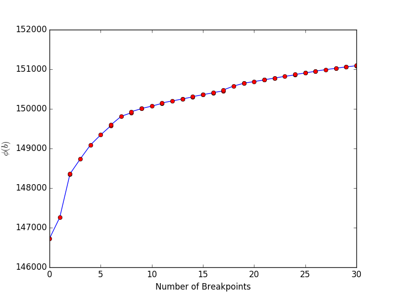
Figure 2: Objective $\phi(b)$ vs. number of breakpoints $K$ for $\lambda=10^{-4}$.

Figure 3: Average train and test set log-likelihood during 10-fold cross validation for various $\lambda$’s and across all values of $K\leq 30$.

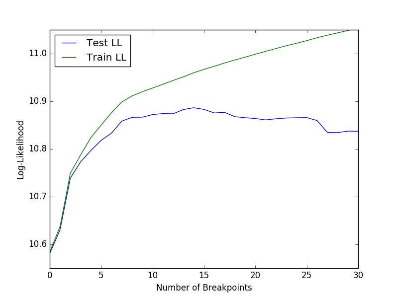
(a) $\lambda=10^{-6}$

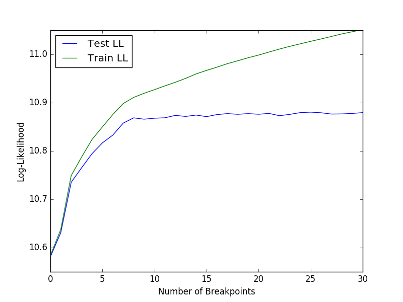
(b) $\lambda=10^{-5}$

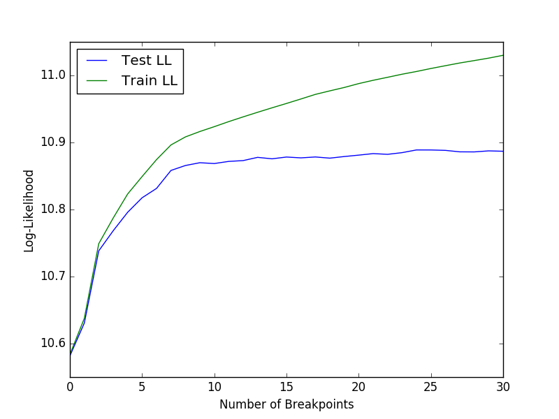
(c) $\lambda=10^{-4}$

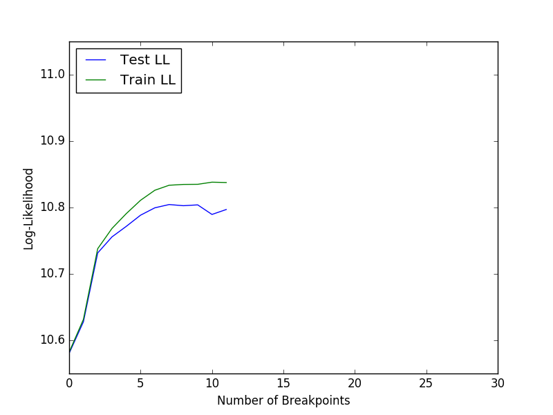
(d) $\lambda=10^{-3}$

Cross-validation.

We next use 10-fold cross-validation to determine reasonable values for $K$ and $\lambda$. We plot the average log-likelihood over the 10 folds versus $K$ in Figure 3(d) for various values of $\lambda$. When $\lambda$ is large, the curves stop before $K=K^{\mathrm{max}}$, since GGS terminates early. These plots clearly show that increasing $K$ above 10 does not increase the average log-likelihood in the test set; and moreover past this point the log-likelihood on the test and training sets begin to diverge, meaning the model is overfit. Though Figure 3(d) only goes up to $K=30$, we find that for values of $K$ above around 60, the log-likelihood begins to drop significantly. Furthermore, we see that values of $\lambda$ up to $\lambda=10^{-4}$ yield roughly the same high log-likelihood. This suggests that choices of $K=10$ and $\lambda=10^{-4}$ are reasonable, aligning with our general preference for models which are simple (small $K$) and not too sensitive to noise (large $\lambda$). Cross-validation also reveals that the choice of breakpoint locations is very stable for these values of $K$ and $\lambda$, across the 10 folds.

Results.

Figure 4 shows the model obtained by GGS with $\lambda=10^{-4}$ and $K=10$. We plot the covariance matrix by showing the square root of the diagonal entries (i.e., the volatilities), and the three correlations, versus $t$. During the financial crisis in 2008, the mean return of stocks and oil was very negative and the volatility was high. The stock market and the oil price were almost uncorrelated before 2008, but have been positively correlated since then. It is interesting to see how the correlation between stocks and bonds has varied over time: It was strongly positive in 1997 and very negative in 1998, in 2002, and in the five years from mid-2007 to mid-2012. The sudden shift in this correlation between 1997 and 1998 is why GGS yields two relatively short segments in the [1997, 1999] window, rather than breaking up a longer segment (such as [1999, 2002], where the correlation structure is more homogenous). The extent of these variations would be difficult to capture using a sliding window; the window would have to be very short, which would lead to noisy estimates. The segmentation approach yields a more interpretable partitioning with no dependence on a (prespecified, fixed) window length. Approaches to risk modeling [Ale00] and portfolio optimization [PC04, Meu09] based on principal component analysis are questionable, when volatilities and correlations are changing as significantly as is the case in Figure 4 (see also [FPW⁺11]). We plot the cumulative index returns along with the chosen breakpoints in Figure 5. We can clearly see natural segments and boundaries, for example the Russian default in 1998 and the 2008 financial crisis.

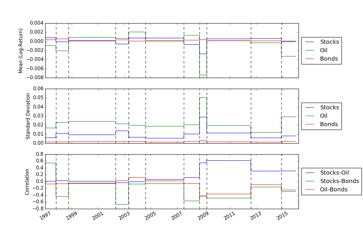
Figure 4: Segmented Gaussian model obtained with $\lambda=10^{-4}$, $K=10$.

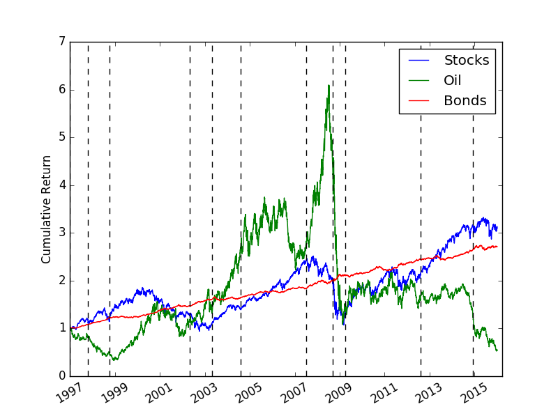
Figure 5: Cumulative returns with vertical bars at the model breakpoints.

Comparison with random warm-start.

We fix the hyperparameters $K=10$ and $\lambda=10^{-4}$, and attempt to find a better SGM using warm-start with random breakpoints. This step is not needed; we carry this out to demonstrate that while GGS does not find the model that globally maximizes the objective, it is effective. We run 10000 warm-start random initial breakpoint computations, running AdjustBreakpoints until the model is 1-OPT and computing the objective found in each case. (In this case the number of passes over the data set far exceeds two, the typical number in GGS.) The complementary CDF of the objective for these 10000 computations is shown in Figure 6, as well as the objective values found by GGS for $K=8$ through $K=11$. We see that the random initializations can sometimes lead to very poor results; over 50% of the simulations, even though they are locally optimal, have smaller objectives than the $K=9$ step of GGS. On the other hand, the random initializations do find some SGMs with objective slightly exceeding the one found by GGS, demonstrating that GGS did not find the globally optimal set of breakpoints. These SGMs have similar breakpoints, and similar cross-validated log-likelihood, as the one found by GGS. As a practical matter, these SGMs are no better than the one found by GGS. There are two advantages of GGS over the random search: First, it is much faster; and second, it finds models for a range of values of $K$, which is useful before we select the value of $K$ to use.

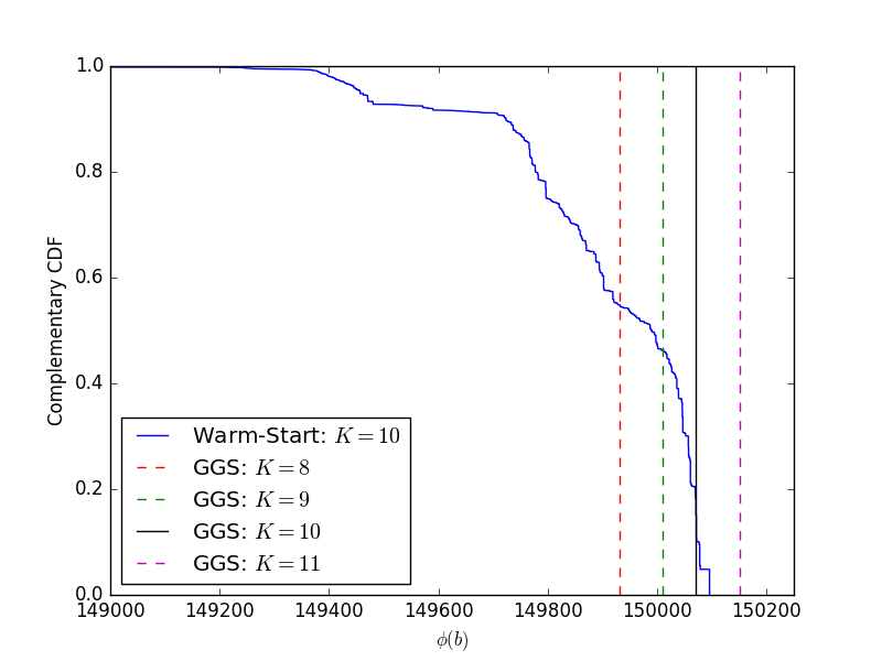
Figure 6: Empirical complementary CDF of $\phi(b)$ for 10000 randomly initialized results for $K=10$, $\lambda=10^{-4}$. Vertical bars represent GGS solutions for different values of $K$.

6.3 Large-scale financial example

Data set description.

We next look at a larger example to emphasize the scalability of GGS. We look at all companies currently in the S&P 500 index that have been publicly listed for the entire 19-year interval from before (from 1997 to 2015), which leaves 309 companies. Note that there are slightly fewer trading days for the S&P 500 each year than the global indices, since the S&P 500 does not trade during US holidays, while the global indices still move. The 19-year data set yields a $309\times 4782$ data matrix. We take daily log-returns for these stocks, and run the GGS algorithm to detect relevant breakpoints.

GGS scalability.

We run GGS on this much larger data set up to $K^{\mathrm{max}}=10$. Our serial implementation of the GGS algorithm, on the same 1.7 GHz Intel i7 processor, took 36 minutes, where AdjustBreakpoint took an average of 3.5 passes through the data at each $K$. Note that this aligns very closely with our predicted runtime from §3.2, which was estimated as $(K^{\mathrm{max}})^{2}LTn$.

Cross-validation.

We run 10-fold cross-validation to find good values of the hyperparameters $K$ and $\lambda$. The average log-likelihood of the test and train sets are displayed in Figure 7(d). From the results, we can see that the log-likelihood is maximized at a much smaller value of $K$, indicating fewer breakpoints. This is in part because, with $n=309$, we need more samples in each segment to get an accurate estimate of the $309\times 309$ covariance matrix, as opposed to the $3\times 3$ covariance in the smaller example. Our cross-validation results suggest choosing $K=3$ and $\lambda=5\times 10^{-2}$, and as in the small example, the results are very stable near these values.

Figure 7: Average train and test set log-likelihood during 10-fold cross validation for various $\lambda$’s for the 309-stock example. Note that not all $\lambda$’s go all the way up to $K=10$ because our algorithm stops when it determines that it will no longer benefit from adding an additional split.

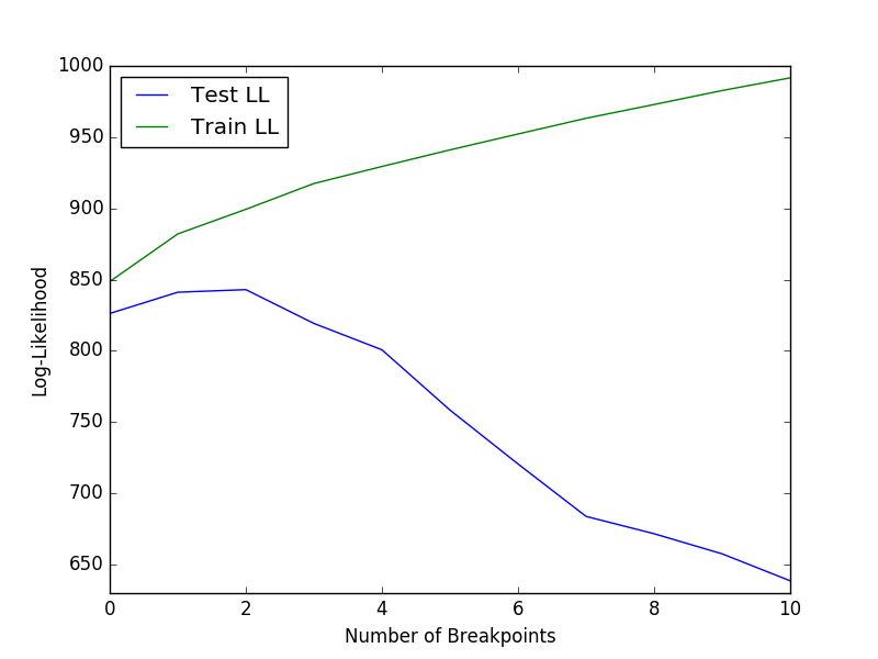
(a) $\lambda=5\times 10^{-3}$

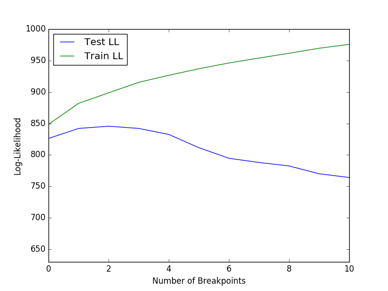
(b) $\lambda=10^{-2}$

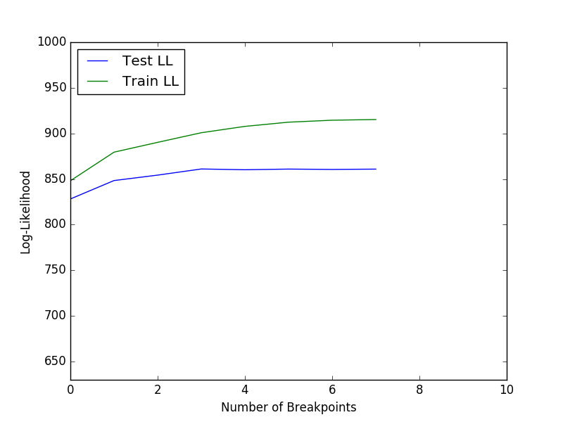
(c) $\lambda=5\times 10^{-2}$

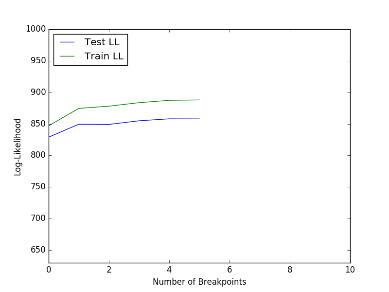
(d) $\lambda=10^{-1}$

Results.

We plot the mean, standard deviation, and cumulative return of a uniform, buy-and-hold portfolio (i.e., investing $1 into each of the 309 stocks in 1997). The results are shown in Figure 8. Note that there is a selection bias in the data set, since these companies all remained in the S&P 500 in 2016, and the total return is 8x over the 19-year interval. Like before, the 2008 financial crisis stands out. It is the only segment with a negative mean value. The partitioning seems intuitively right. The first, highly volatile, segment includes both the build-up and burst of the dot–com bubble. The second segment is the bull market that led to the financial crisis in 2008. The third segment is the financial crisis and the fourth segment is the market rally that followed the crisis. These break points were also found in the multiasset example in Figure 4 and 5.

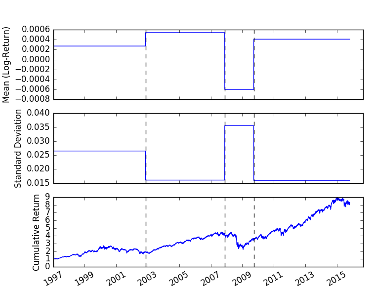
Figure 8: Mean, standard deviation, and cumulative return for a uniform portfolio with $K=3$, $\lambda=5\times 10^{-2}$.

6.4 Wikipedia text data

We examine an example from the field of natural language processing (NLP) to illustrate how GGS can be applied to a very different type of data set, beyond traditional time series examples.

Data set description.

We look at text data from English-language Wikipedia. We obtain our data by concatenating the introductions, i.e., the text that precedes the Table of Contents section on the Wikipedia webpage, of five separate articles, with titles George Clooney, Botany, Julius Caesar, Jazz, and Denmark. Here, the “time series” consists of the sequence of words from these five articles in order. After basic preprocessing (removing words that appear at least five times and in multiple articles), our data set consists of 1282 words, with each article contributing between 224 and 286 words. We then convert each word into a 300-dimensional vector using a pretrained Word2Vec embedding of three million unique words (or short phrases), trained on the Google News data set of approximately 100 billion words, available at

https://code.google.com/archive/p/word2vec/.

This leaves us with a $300\times 1282$ data matrix. Our hope is that GGS can detect the breakpoints between the five concatenated articles, based solely on the change in mean and covariance of the vectors associated with the words in our vector series.

GGS results.

We run GGS to split the data into five segments — i.e., $K=4$ — and use cross-validation to select $\lambda=10^{-3}$. (We note, however, that this example is quite robust to the selection of $\lambda$, and any value from $10^{-6}$ to $10^{-3}$ yields the exact same breakpoint locations.) We plot the results in Figure 9, which show GGS achieving a near-perfect split of the five articles. Figure 9 also shows a representative word (or short phrase) in the Google News data set that is among the top five “most similar” words, out of the entire three million word corpus, to the average (mean) of each GGS segment, as measured by cosine similarity. We see that GGS correctly identifies both the breakpoint locations and the general topic of each segment.

Figure 9: Actual and GGS predicted breakpoints for the concatenation of the five Wikipedia articles, along with the predicted most similar word to the mean of each GGS segment.

6.5 Comparison with left-to-right HMM on synthetic data

We next analyze a synthetic example where observations are generated from a given sequence of segments. This provides a known ground truth, allowing us to compare GGS with a common baseline, a left-to-right hidden Markov model (HMM) [Bak76, CMR05]. Left-to-right HMMs, like GGS, split the data into non-repeatable segments, where each segment is defined by a Gaussian distribution. The HMMs in this experiment are implemented using the rarhsmm library [XL17], which includes the same shrinkage estimator for the covariance matrices used in GGS (see §2.2). The shrinkage estimator results in more reliable estimates not only of the covariance matrices but also of the transition matrix and the hidden states [FFvSK17].

Data set description.

We start by generating 10 random covariance matrices. We do so by setting $\Sigma_{i}=A^{(i)}A^{(i)T},i=1,\ldots,10$, where $A^{(i)}\in{\mbox{\bf R}}^{25\times 25}$ is a random matrix where each element $A^{(i)}_{j,k}$ was generated independently from the standard normal distribution. Our synthetic data set then has 10 ground truth segments (or $K=9$ breakpoints), where segment $i$ has zero mean and covariance $\Sigma_{i}$. Each segment is of length 100 (so the total time series has $T=1000$ observations). Each of the 100 readings per segment is sampled independently from the given distribution. Thus, our final data set consists of a 25 $\times$ 1000 data matrix, consisting of 10 independent segments, each of length 100.

Results.

We run both GGS and the left-to-right HMM on this data set. For GGS, we immediately notice a kink in the objective at $K=9$, as shown in Figure 10(a), indicating that the data should be split into $K+1=10$ segments. We use cross-validation to choose an appropriate value of $\lambda$, which yields $\lambda=10$. We plot the train and test set log-likelihoods at $\lambda=10$ in Figure 10(b). (Similar to the Wikipedia text example, though, the breakpoint locations are relatively robust to our selection of $\lambda$. GGS returns identical breakpoints for any $\lambda$ between $10^{-3}$ and $10^{3}$). For this value of $\lambda$ (and thus for the whole range of $\lambda$ between $10^{-3}$ and $10^{3}$), we split the data perfectly, identifying the nine breakpoints at their exact locations.

Left-to-right HMMs have various methods for determining the number of segments, such as AIC or BIC. Here we instead simply use the correct number of segments, and initialize the transition matrix as its true value. Note that this is the best-case scenario for the left-to-right HMM. Even with this advantage, the left-to-right HMM struggles to properly split the time series. Whereas GGS correctly identifies $[100,200,300,400,500,600,700,800,900]$ as the breakpoints, the left-to-right HMM gets at least one breakpoint completely wrong (and splits the data at, for example, $[100,200,300,400,500,600,663,700,800]$).

These results are consistent. In fact, when this experiment was repeated 100 times (with different randomly generated data), GGS identified the correct breakpoints every single time. We also note that GGS is robust to $n$ (the dimension of the data), $K$ (the number of breakpoints), and $T/(K+1)$ (the average segment length), perfectly splitting the data at the exact breakpoints for all tests across at least one order of magnitude in each of these three parameters. On the other hand, the 100 left-to-right HMM experiments correctly labeled on average just 7.46 of the nine true breakpoints (and never more than eight). In these HMM experiments, instead of ten segments of length 100, the shortest segment had an average length of 26, and the longest segment had an average length of 200. Additionally, the left-to-right HMM struggles as the parameters change, performing even worse when $K$ increases and when $T/(K+1)$ is small compared to $n$ (though formal analysis of the robustness of left-to-right HMMs is outside the scope of this paper). This comes as no surprise, because finding the global maximum among all local maxima of the likelihood function for an HMM with many states is known to be difficult problem [CMR05, Chapter 1.4]. Therefore, as shown by these these experiments, GGS appears to outperform left-to-right HMMs in this setting.

Figure 10: GGS correctly identifies that there are 10 underlying segments in the data (from the kink in the plots at $K=9$).

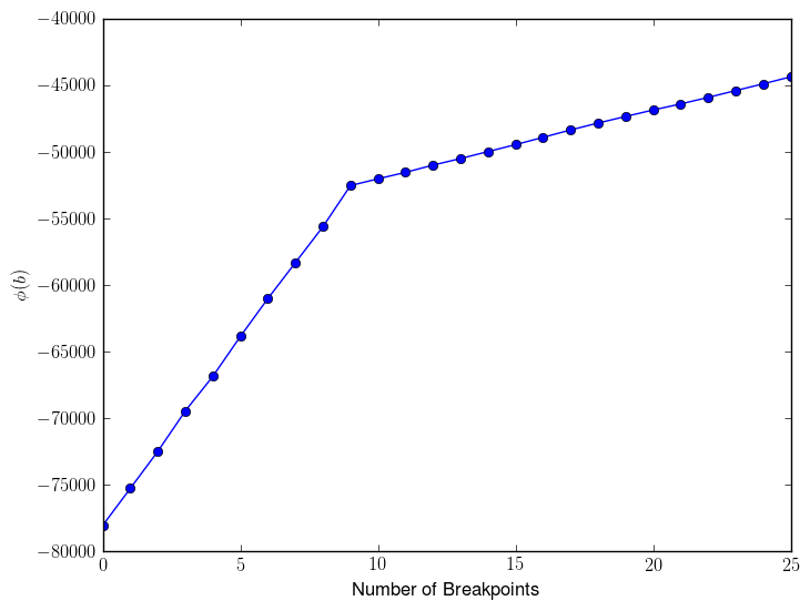
(a) Objective vs. breakpoints for $\lambda=10$.

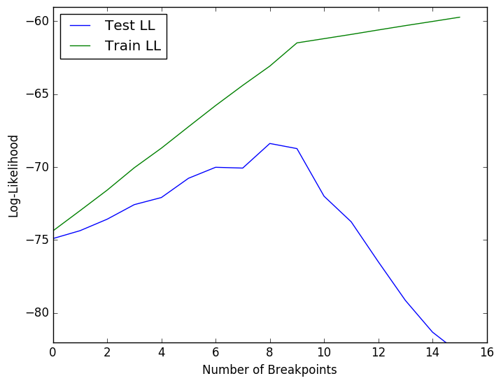
(b) Average train/test log-likelihood for $\lambda=10$.

7 Summary

We have analyzed the problem of breaking a multivariate time series into segments, where the data in each segment could be modeled as independent samples from a multivariate Gaussian distribution. Our greedy Gaussian segmentation (GGS) algorithm is able to approximately maximize the covariance-regularized log-likelihood in an efficient manner, easily scaling to vectors with dimension over 1000 and time series of any length. Examples on both small and large data sets yielded useful insights. Our implementation, available at https://github.com/cvxgrp/GGS, can be used to solve problems in a variety of applications. For example, the regularized parameter estimates obtained by GGS could be used as inputs to portfolio optimization, where correlations between different assets play an important role when determining optimal holdings.

References

- [AFNA05] J. Abonyi, B. Feil, S. Nemeth, and P. Arva. Modified Gath–Geva clustering for fuzzy segmentation of multivariate time-series. Fuzzy Sets and Systems, 149(1):39–56, 2005.
- [Ale00] C. Alexander. A primer on the orthogonal GARCH model. Unpublished manuscript, ISMA Center, University of Reading, U.K., 2000.
- [AT12] A. Ang and A. Timmermann. Regime changes and financial markets. Annual Review of Financial Economics, 4(1):313–337, 2012.
- [Bak76] R. Bakis. Continuous speech recognition via centisecond acoustic states. Journal of the Acoustical Society of America, 59(S1):S97, 1976.
- [Bel61] R. Bellman. On the approximation of curves by line segments using dynamic programming. Communications of the ACM, 4(6):284, 1961.
- [BL08] P. J. Bickel and E. Levina. Regularized estimation of large covariance matrices. Annals of Statistics, 36(1):199–227, 2008.
- [BN93] M. Basseville and I. V. Nikiforov. Detection of Abrupt Changes: Theory and Application, volume 104. Prentice Hall: Englewood Cliffs, 1993.
- [BR12] L. Bauwens and J. Rombouts. On marginal likelihood computation in change-point models. Computational Statistics & Data Analysis, 56(11):3415–3429, 2012.
- [BS82] N. B. Booth and A. F. M. Smith. A Bayesian approach to retrospective identification of change-points. Journal of Econometrics, 19(1):7–22, 1982.
- [BU08] E. Borenstein and S. Ullman. Combined top-down/bottom-up segmentation. IEEE Transactions on Pattern Analysis and Machine Intelligence, 30(12):2109–2125, 2008.
- [Bul11] J. Bulla. Hidden Markov models with components. Increased persistence and other aspects. Quantitative Finance, 11(3):459–475, 2011.
- [BV11] K. Bleakley and J.-P. Vert. The group fused lasso for multiple change-point detection. arXiv preprint arXiv:1106.4199, 2011.
- [CD03] A. Chouakria-Douzal. Compression technique preserving correlations of a multivariate temporal sequence. In M. R. Berthold, H.-J. Lenz, E. Bradley, R. Kruse, and C. Borgelt, editors, Advances in Intelligent Data Analysis V, volume 2810 of Lecture Notes in Computer Science, pages 566–577. Springer: Berlin, 2003.
- [CK10] S. Cheon and J. Kim. Multiple change-point detection of multivariate mean vectors with the Bayesian approach. Computational Statistics & Data Analysis, 54(2):406–415, 2010.
- [CMR05] O. Cappé, E. Moulines, and T. Rydén. Inference in Hidden Markov Models. Springer: New York, 2005.
- [Cro88] R. B. Crosier. Multivariate generalizations of cumulative sum quality-control schemes. Technometrics, 30(3):291–303, 1988.
- [CWB08] E. J. Candès, M. B. Wakin, and S. Boyd. Enhancing sparsity by reweighted minimization. Journal of Fourier Analysis and Applications, 14(5–6):877–905, 2008.
- [DG06] J. De Gooijer. Detecting change-points in multidimensional stochastic processes. Computational Statistics & Data Analysis, 51(3):1892–1903, 2006.
- [DP73] D. H. Douglas and T. K. Peucker. Algorithms for the reduction of the number of points required to represent a digitized line or its caricature. Cartographica: The International Journal for Geographic Information and Geovisualization, 10(2):112–122, 1973.
- [EA12] P. Esling and C. Agon. Time-series data mining. ACM Computing Surveys, 45(1):12, 2012.
- [FFvSK17] M. Fiecas, J. Franke, R. von Sachs, and J. T. Kamgaing. Shrinkage estimation for multivariate hidden Markov models. Journal of the American Statistical Association, 112(517):424–435, 2017.
- [FPK04] P. Fragkou, V. Petridis, and A. Kehagias. A dynamic programming algorithm for linear text segmentation. Journal of Intelligent Information Systems, 23(2):179–197, 2004.
- [FPW+11] D. J. Fenn, M. A. Porter, S. Williams, M. McDonald, N. F. Johnson, and N. S. Jones. Temporal evolution of financial-market correlations. Physical Review E, 84(2):026109, 2011.
- [GS99] V. Guralnik and J. Srivastava. Event detection from time series data. In Proceedings of the Fifth ACM SIGKDD International Conference on Knowledge Discovery and Data Mining, pages 33–42, 1999.
- [GS01] X. Ge and P. Smyth. Segmental semi-Markov models for endpoint detection in plasma etching. IEEE Transactions on Semiconductor Engineering, 259:201–209, 2001.
- [Gus00] F. Gustafsson. Adaptive Filtering and Change Detection. Wiley: West Sussex, 2000.
- [GW14] P. Galeano and D. Wied. Multiple break detection in the correlation structure of random variables. Computational Statistics & Data Analysis, 76:262–282, 2014.
- [HLPL06] J. Z. Huang, N. Liu, M. Pourahmadi, and L. Liu. Covariance matrix selection and estimation via penalised normal likelihood. Biometrika, 93(1):85–98, 2006.
- [HRH+15] B. Hu, T. Rakthanmanon, Y. Hao, S. Evans, S. Lonardi, and E. Keogh. Using the minimum description length to discover the intrinsic cardinality and dimensionality of time series. Data Mining and Knowledge Discovery, 29(2):358–399, 2015.
- [HSS+16] D. Hallac, A. Sharang, R. Stahmann, A. Lamprecht, M. Huber, M. Roehder, R. Sosič, and J. Leskovec. Driver identification using automobile sensor data from a single turn. In IEEE 19th International Conference on Intelligent Transport Systems, pages 953–958, 2016.
- [HTF09] T. Hastie, R. Tibshirani, and J. Friedman. The Elements of Statistical Learning. Springer: New York, 2nd edition, 2009.
- [KC14] I. Katz and K. Crammer. Outlier-robust convex segmentation. arXiv preprint arXiv:1411.4503, 2014.
- [KCHP04] E. Keogh, S. Chu, D. Hart, and M. Pazzani. Segmenting time series: A survey and novel approach. In M. Last, A. Kandel, and H. Bunke, editors, Data Mining in Time Series Databases, volume 57 of Series in Machine Perception and Artificial Intelligence, chapter 1. World Scientific: Singapore, 2004.
- [KKBG09] S.-J. Kim, K. Koh, S. Boyd, and D. Gorinevsky. trend filtering. SIAM Review, 51(2):339–360, 2009.
- [KNP06] A. Kehagias, E. Nidelkou, and V. Petridis. A dynamic programming segmentation procedure for hydrological and environmental time series. Stochastic Environmental Research and Risk Assessment, 20(1):77–94, 2006.
- [Lee98] C.-B. Lee. Bayesian analysis of a change-point in exponential families with applications. Computational Statistics & Data Analysis, 27(2):195–208, 1998.
- [LH15] J. Lee and T. Hastie. Learning the structure of mixed graphical models. Journal of Computational and Graphical Statistics, 24(1):230–253, 2015.
- [Li15] J. Li. Nonparametric multivariate statistical process control charts: a hypothesis testing-based approach. Journal of Nonparametric Statistics, 27(3):383–400, 2015.
- [LW04] O. Ledoit and M. Wolf. A well-conditioned estimator for large-dimensional covariance matrices. Journal of Multivariate Analysis, 88(2):365–411, 2004.
- [Meu09] A. Meucci. Managing diversification. Risk, 22(5):74–79, 2009.
- [NHL+17] P. Nystrup, B. W. Hansen, H. O. Larsen, H. Madsen, and E. Lindström. Dynamic allocation or diversification: A regime-based approach to multiple assets. Journal of Portfolio Management, 44(2):62–73, 2017.
- [NHML15] P. Nystrup, B. W. Hansen, H. Madsen, and E. Lindström. Regime-based versus static asset allocation: Letting the data speak. Journal of Portfolio Management, 42(1):103–109, 2015.
- [NHML16] P. Nystrup, B. W. Hansen, H. Madsen, and E. Lindström. Detecting change points in VIX and S&P 500: A new approach to dynamic asset allocation. Journal of Asset Management, 17(5):361–374, 2016.
- [NML17] P. Nystrup, H. Madsen, and E. Lindström. Long memory of financial time series and hidden Markov models with time-varying parameters. Journal of Forecasting, 36(8):989–1002, 2017.
- [PC04] M. H. Partovi and M. Caputo. Principal portfolios: Recasting the efficient frontier. Economics Bulletin, 7(3):1–10, 2004.
- [PLBR11] F. Picard, É. Lebarbier, E. Budinská, and S. Robin. Joint segmentation of multivariate Gaussian processes using mixed linear models. Computational Statistics & Data Analysis, 55(2):1160–1170, 2011.
- [RR06] V. Rajagopalan and A. Ray. Symbolic time series analysis via wavelet-based partitioning. Signal Processing, 86(11):3309–3320, 2006.
- [RTÅ98] T. Rydén, T. Teräsvirta, and S. Åsbrink. Stylized facts of daily return series and the hidden Markov model. Journal of Applied Econometrics, 13(3):217–244, 1998.
- [SCGA11] A. Samé, F. Chamroukhi, G. Govaert, and P. Aknin. Model-based clustering and segmentation of time series with changes in regime. Advances in Data Analysis and Classification, 5(4):301–321, 2011.
- [SK05] Y. S. Son and S. Kim. Bayesian single change point detection in a sequence of multivariate normal observations. Statistics, 39(5):373–387, 2005.
- [SS12] A. Sheikh and J. Sun. Regime change: Implications of macroeconomic shifts on asset class and portfolio performance. Journal of Investing, 21(3):36–54, 2012.
- [TPSR15] W. Tansey, O. H. M. Padilla, A. S. Suggala, and P. Ravikumar. Vector-space Markov random fields via exponential families. In Proceedings of the 32nd International Conference on Machine Learning, volume 1, pages 684–692, 2015.
- [TSR+05] R. Tibshirani, M. Saunders, S. Rosset, J. Zhu, and K. Knight. Sparsity and smoothness via the fused lasso. Journal of the Royal Statistical Society: Series B (Statistical Methodology), 67(1):91–108, 2005.
- [VS96] J. H. Venter and S. J. Steel. Finding multiple abrupt change points. Computational Statistics & Data Analysis, 22(5):481–504, 1996.
- [VVK03] J. Verbeek, N. Vlassis, and B. Kröse. Efficient greedy learning of Gaussian mixture models. Neural Computation, 15(2):469–485, 2003.
- [WBAW12] B. Wahlberg, S. Boyd, M. Annergren, and Y. Wang. An ADMM algorithm for a class of total variation regularized estimation problems. IFAC Proceedings Volumes, 45(16):83–88, 2012.
- [Wel62] B. P. Welford. Note on a method for calculating corrected sums of squares and products. Technometrics, 4(3):419–420, 1962.
- [WRA11] B. Wahlberg, C. Rojas, and M. Annergren. On mean and variance filtering. In Proceedings of the Forty Fifth Asilomar Conference on Signals, Systems and Computers, pages 1913–1916, 2011.
- [WT09] D. Witten and R. Tibshirani. Covariance-regularized regression and classification for high dimensional problems. Journal of the Royal Statistical Society: Series B (Statistical Methodology), 71(3):615–636, 2009.
- [XL17] Z. Xu and Y. Liu. Regularized autoregressive hidden semi Markov model. https://github.com/cran/rarhsmm, 2017.
- [Xu02] N. Xu. A survey of sensor network applications. IEEE Communications Magazine, 40(8):102–114, 2002.
- [ZG81] W. I. Zangwill and C. B. Garcia. Pathways to solutions, fixed points, and equilibria. Prentice Hall: Englewood Cliffs, 1981.