Using Machine Learning to Detect Noisy Neighbors in 5G Networks

Abstract

5G networks are expected to be more dynamic and chaotic in their structure than current networks. With the advent of Network Function Virtualization (NFV), Network Functions (NF) will no longer be tightly coupled with the hardware they are running on, which poses new challenges in network management. Noisy neighbor is a term commonly used to describe situations in NFV infrastructure where an application experiences degradation in performance due to the fact that some of the resources it needs are occupied by other applications in the same cloud node. These situations cannot be easily identified using straightforward approaches, which calls for the use of sophisticated methods for NFV infrastructure management. In this paper we demonstrate how Machine Learning (ML) techniques can be used to identify such events. Through experiments using data collected at real NFV infrastructure, we show that standard models for automated classification can detect the noisy neighbor phenomenon with an accuracy of more than 90% in a simple scenario.

I Introduction

5G networks are expected to be inherently more dynamic and chaotic in their structure than current networks. With the advent of Network Function Virtualization (NFV), Network Functions (NF) will no longer be tightly coupled with the hardware they are running on. Instead, when considering network design and management a decade into the future, it is believed that many NFs will be virtualized, and thus able to be deployed, scaled and migrated with ease and speed unheard of in today’s networks. As a result, while the topology of the physical network infrastructure shall evolve on a slow time scale similar to that of current networks, the dynamics of the virtual/logical topology will undergo a dramatic change and be allowed to evolve at much faster speeds, in service of customer needs and demands.

When considering network management in such an environment, achieving the degree of reliability and stability that is to be expected of 5G becomes a challenge. Specifically, when the network topology is in constant flux, it is more difficult to make decisions regarding where to locate services, ensure the SLA a provider is committed to, and perform Root Cause Analysis (RCA) on system faults. One specific challenge in this domain is the problem of allocating network resources in a dynamically changing environment like NFV [2]. This challenge relates to the problem of service demand prediction and provisioning which allows the network to resize and resource itself, using virtualization, to serve predicted demand according to parameters such as location, time and specific service demand from specific users or user groups.

The more specific issues we will address in this paper is identifying the state of a service and the reason for this state. More specifically we want to identify that the service is facing difficulties and identify the cause of these difficulties. This is a critical building block in addressing use cases similar to the “Optimized Services in Dynamic Environments” use case described in [10]. Noisy neighbor is a term commonly used to describe situations in cloud computing where an application (or a VM) experiences degradation in performance due to the fact that some of the resources it needs are occupied by other applications (VMs) in the same cloud node. Note that in general there should be a clear separation between the different tenants on the same physical machine, but in practice this isolation of the virtual machines is far from perfect and many resources such as internal networking resources and memory access resources are shared at some level. In this paper we demonstrate how Machine Learning (ML) techniques can be used to identify such events. We show that using standard models for automated classification, noisy neighbors can be detected in a simple scenario with more than 90% accuracy. As said this is a critical building block in creating flexible reliable orchestration mechanisms for 5G networks as once identified, the system can resolve the performance issue by migrating one of the tenants to another machine or by allocating more resources. The rest of the paper is structured as folows: section II describes the problem setting in detail. Section III describes the employed machine learning models. Section IV provides experimental results and finally section V outlines future work and offers concluding remarks.

II Problem setting

This testbed environment consists of a total of five high performance HP servers (each having 12 cores) with a proprietary management system running on top of an OpenStack cloud [3]. Two of the servers are dedicated to the management processes, while the other three are available as compute machines.

An open source voice-over-IP (VoIP) application, Asterisk [1], is deployed on one of the compute machines, in a single virtual machine utilizing one core and 1024 MB of memory. A corresponding traffic generator, SipP [4] is deployed in a second machine, and configured to log in and log out of the server, and initiate calls to a line in which the server is playing music-on-hold. The traffic generator is configured in a manner that generates constant reasonable load on the server, e.g. 40% CPU utilization.

Another application that was considered is a Fibonacci server – a specially-tailored application, designed to mimic Virtual Network Functions in behaviour, but be simple enough for experimentation and analysis. The server computes elements in the Fibonacci series on demand. A client may request the index of the element to be computed. Different implementations of the server are considered, to examine the noisy neighbour effect on them.

A noisy neighbour is defined as (one or more) virtual machines (VMs) sharing resources with the server under test, thus affecting its performance. Since both of the servers under test are CPU intensive, we focused on CPU noise. Noise was generated using the ”stress” Linux application. In its CPU-intensive setting, it continuously computes square-roots of numbers in order to generate load on CPUs. Noise is therefore simulated by further noise generation virtual machines, all launched on the same server as the VoIP server. We experimented with both a single large VM occupying all physical CPUs, as well as multiple small VMs, each occupying only one or two cores. During experimentations, the following metrics were collected:

• CPU utilization of the server VM

• In-bound network traffic of the server VM

• Out-bound network traffic of the server VM

• CPU utilization of the noise VM(s). The purpose of this metric is to act as an indicator of whether noise exists or not, for the ML training period

Monitoring is performed using Openstack Ceilometer, and the data is collected by the proprietary management system into a DB for further analysis and extraction. Experimentations differ in the following attributes:

• Server under test: Asterisk vs. Synthetic

• Amount of noise: One VM utilizing all 24 cores vs. several (between 18 and 24) utilizing a single core each.

• Amount of traffic generated (and respectively amount of CPU utilization in the server)

III Machine learning methods

The problem of determining whether or not the behavior of a virtual machine is being caused by the presence of a noisy neighbor is non-trivial. Based on the metrics described above, a simple thresholding approach or a set of rules would not suffice.

Therefore, to address this problem we propose the use of machine learning methods. Machine learning has proved successful in a wide variety of domains, such as computer vision [15] [11], bioinformatics [17], natural language processing [12][16] and others. A key advantage of machine learning is that the same models can be applied to completely different domains provided that the data are transformed into an adequate representation.

In this paper we address the problem of determining whether or not a noisy neighbor situation is taking place, which can be modelled in machine learning as a classification problem. Hence, we propose to employ two well-known classifiers: support vector machines and random forests.

III-A Support vector machines

Given a set of data points represented as real-valued vectors corresponding to two different classes, support vector machines (SVM) [9] pose the problem of finding a maximum-margin separating hyperplane. It can be shown that this is equivalent to minimizing the norm of the vector orthogonal to said hyperplane, constraining the data points of different classes to be on different sides and at a minimum distance from it. Formally, this can be formulated as follows.

Given a set of data points $\{x_{1},\dots,x_{n}\}$ and corresponding labels $\{y_{1},\dots,y_{n}\}$, where $x_{i}\in\mathbb{R}^{d}$ and $y_{i}\in\{-1,1\}$, $i=1,\dots,n$, for some $d\in\mathbb{N}$, find

$$\underset{w}{\text{min}} \frac{1}{2}\|w\|^{2}+C\sum_{i}{\xi_{i}}$$ (1)

s.t. $$y_{i}(wx_{i})\geq 1-\xi_{i}\mbox{ },i=1,\dots,n$$

$$\xi_{i}\geq 0\mbox{ }i=1,\dots,n$$

Here, we introduce slack variables $\xi_{i}$, which allow for violations of the separation constraint. This formulation is often referred to as soft-margin SVM. The variable $C\in\mathbb{R}$ is a hyperparameter that allows us to control the amount of penalization incurred by these violations.

In the case of support vector machines, strong duality holds [6]. Therefore, a Lagrangian can be formulated such that its maximum value provides the solution to our problem. Optimizing with respect to the corresponding variables yields the following formulation.

$$\underset{\alpha}{\text{max}} \sum_{i}\alpha_{i}-\frac{1}{2}\sum_{i}\sum_{j}\alpha_{i}\alpha_{j}y_{i}y_{j}\langle x_{i},x_{j}\rangle$$ (2)

s.t. $$\sum_{i}y_{i}\alpha_{i}=0$$

$$0\leq\alpha_{i}\leq C\mbox{ }i=1,\dots,n$$

Here, $\alpha_{i}$, $i=1,\dots,n$ are the Lagrange multipliers corresponding to the inequality constraint of the primal formulation.

The sole dependence of this formulation on the inner products allows for the use of a technique often referred to as the kernel trick [5]. Kernel functions implicitly map vectors to a higher dimensional space and compute their inner product. This enables learning separating hyperplanes for non-separable data.

III-B Random forests

Random forests [8] are a learning model that combines decision trees with the concept of bagging [7] and random feature selection. Random forests are widely popular because of their simplicity, efficiency and effectiveness.

Random forests function by combining bagging, or bootstrap aggregation, with decision trees. Specifically a number of random samples with replacement is drawn from the data set and a decision tree is trained for each one of them. The final decision for classifying an unseen data instance is taken by majority vote of the trained decision trees. Decision trees, in turn, are built by constructing a hierarchy of binary split nodes. The criterion to choose the splitting rule for each node is the maximization of information gain based of some measure of entropy.

In addition to the bagging process, random forests also employ random subsets of features. In our case, though, due to the low number of features we limit the model to bagged decision trees.

IV Experimental results

In this section, we describe the experiments carried out in order to assess the validity of machine learning as a method for detecting noisy neighbors, as well as the results obtained.

IV-A Data

We collected the Ceilometer metrics as described in section II, running around 100 experiments of the system described above. The metrics were collected each 10 seconds approximately. These measurements were aggregated into 30 second periods in order to avoid the impact of missing values or irregularities in the sampling frequency. Each of the resulting data points thus represents the average CPU load, inbound and outbound bandwidth of the monitored machine. The corresponding binary label determines whether or not the noisy neighbor was inflicting load during that period. The resulting data set is comprised of 9169 data instances, out of which 3088 correspond to noisy neighbors.

As stated above, detecting noisy neighbors from the available data is non-trivial. To illustrate this fact, Table I shows two different measurements of the relationship between the collected features and the noise value. The first row shows the correlation coefficient between each of the different features and the CPU load of the machine that creates noise. The second row shows the maximal information coefficient (MIC) [14]. It is apparent that none of the available features is sufficiently reliable as a predictor on its own, suggesting that the noisy neighbor phenomenon manifests itself in a complex manner.

Correlation and MIC
	CPU	BW in	BW out
Correlation	0.125	0.477	-0.092
MIC	0.371	0.341	0.306

TABLE I: Correlation and maximal information coefficient between the collected features and the noise.

IV-B Experiments

We train the two models described in section III to automatically classify data instances as corresponding to a noisy neighbor situation or not. The input data is standardized to zero mean and unit variance. In both cases we follow a 10-fold cross validation process. We now describe the specific training procedures for each of the models.

IV-B1 Support vector machines

We train $\ell 1$ soft-margin models with the sequential minimal optimization algorithm [13] using a Gaussian kernel. The Gaussian kernel can be defined as $K(u,v)=e^{-\gamma\|u-v\|^{2}}$, where $\gamma$ is a hyperparameter. We train models using different values of $C$. A quadratic expansion of the features is employed, i.e. each data instance $(x_{1},x_{2},x_{3})$ is transformed into $(x_{1},x_{2},x_{3},x_{1}^{2},x_{2}^{2},x_{3}^{2},x_{1}x_{2},x_{1}x_{3},x_{2}x_{3})$.

IV-B2 Random forests

As stated above, given the small number of features we limit the model to bagged decision trees employing all features. Gini’s diversity index is employed for splitting nodes.

IV-B3 Results

In our experiments, both models attained acceptable levels of classification performance. We measure precision, recall and the F1 score, which are defined as follows

$$\mbox{precision}=\frac{tp}{tp+fp}$$

$$\mbox{recall}=\frac{tp}{tp+fn}$$

$$\mbox{F1 score}=2*\frac{\mbox{precision*recall}}{\mbox{precision+recall}}$$

The models were trained with varying values of certain parameters. In the case of support vector machines, we employed varying values of the parameter $C$ in equation 1. Figure 1 shows how the model behaves as we increase this value. As $C$ approaches infinity, the model becomes closer to the hard-margin variant and the training process becomes more expensive. It can be seen that no significant gains are obtained beyond a value of $C=2^{2}$ (note the root scale for $C$). At a certain point, the model is expected to overfit the training data and thus the errors on test data will increase. In the case of random forests, we train models using different numbers of decision trees. Figure 2 shows how the performance varies as more trees are added to the ensemble. It can be seen that no significant improvement is gained from adding more than 50 trees.

Table II shows the values of the three performance metrics for the best models in terms of F1 score for both SVMs and random forests. The best SVM model was trained with $C=3.8^{2}$. However, the edge over more lenient and thus more efficiently trainedd models is very moderate. The best random forest was trained with 300 trees.

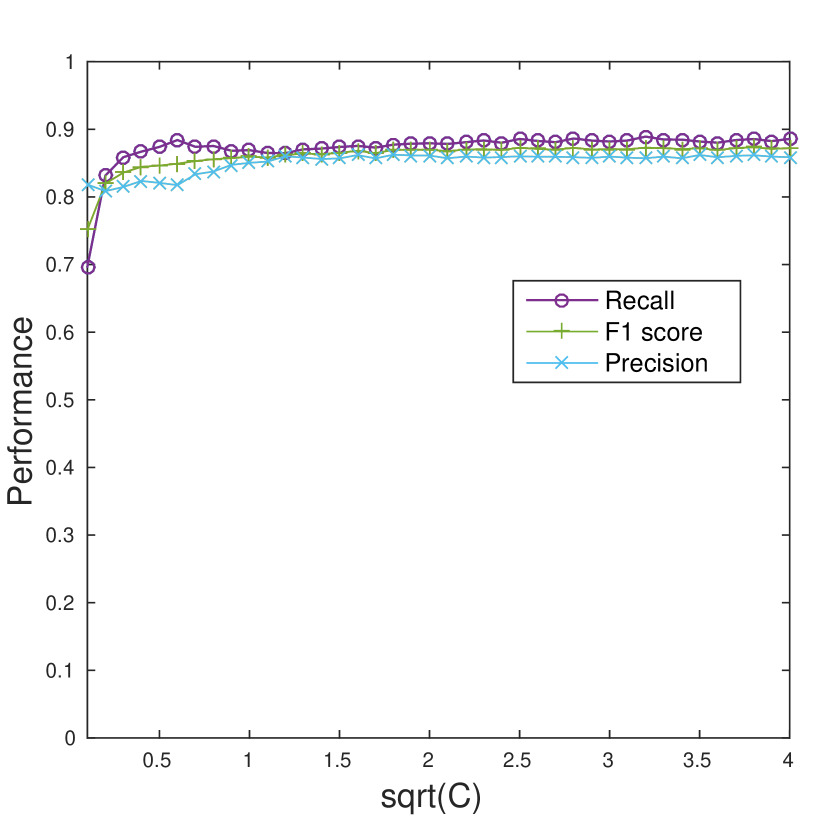
Figure 1: Perfomance of the SVM classifier

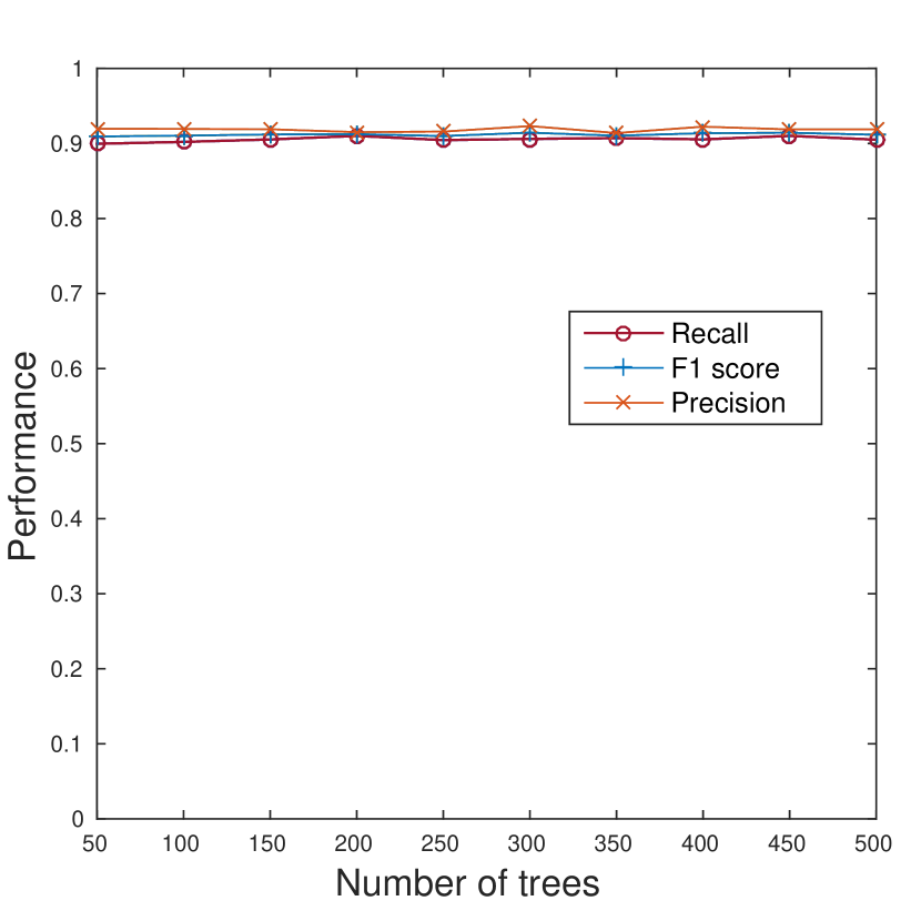
Figure 2: Perfomance of the bagged decision trees

Classification performance
	SVM (C=$3.8^{2}$)	Random forests (300 trees)
Precision	0.8616	0.9232
Recall	0.8856	0.9061
F1 score	0.8734	0.9144

TABLE II: Performance of the best models.

V Conclusions & future work

In this paper we have studied how machine learning can help in managing NFV infrastructure, which is expected to become a prevalent approach in 5G networks. Specifically, we have shown that standard models for classification can detect the noisy neighbor phenomenon with an accuracy of more than 90% in a simple scenario. In the future it would be interesting to evaluate how these models perform in more complex scenarios. It would also be interesting to extract more features from the infrastructure as well as to employ more sophisticated models for improved classification rates.

References

- [1] Asterisk. http://www.asterisk.org/. Accessed: 2016-05-13.
- [2] Network functions virtualisation (nfv); management and orchestration. http://www.etsi.org/deliver/etsi_gs/NFV-MAN/001_099/001/01.01.01_60/gs_nfv-man001v010101p.pdf. Accessed: 2016-05-13.
- [3] Openstack. https://www.openstack.org/. Accessed: 2016-05-13.
- [4] Sipp. http://sipp.sourceforge.net/. Accessed: 2016-05-13.
- [5] Bernhard E Boser, Isabelle M Guyon, and Vladimir N Vapnik. A training algorithm for optimal margin classifiers. In Proceedings of the fifth annual workshop on Computational learning theory, pages 144–152. ACM, 1992.
- [6] Stephen Boyd and Lieven Vandenberghe. Convex optimization. Cambridge university press, 2004.
- [7] Leo Breiman. Bagging predictors. Machine learning, 24(2):123–140, 1996.
- [8] Leo Breiman. Random forests. Machine learning, 45(1):5–32, 2001.
- [9] Corinna Cortes and Vladimir Vapnik. Support-vector networks. Machine learning, 20(3):273–297, 1995.
- [10] T. S. Buda et al. Can machine learning aid in delivering new use cases & scenarios in 5g? In The First IFIP/IEEE International Workshop on Management of 5G Networks, 2016.
- [11] Alex Krizhevsky, Ilya Sutskever, and Geoffrey E Hinton. Imagenet classification with deep convolutional neural networks. In Advances in neural information processing systems, pages 1097–1105, 2012.
- [12] Frederic Morin and Yoshua Bengio. Hierarchical probabilistic neural network language model. In Aistats, volume 5, pages 246–252. Citeseer, 2005.
- [13] John Platt et al. Sequential minimal optimization: A fast algorithm for training support vector machines. 1998.
- [14] David N Reshef, Yakir A Reshef, Hilary K Finucane, Sharon R Grossman, Gilean McVean, Peter J Turnbaugh, Eric S Lander, Michael Mitzenmacher, and Pardis C Sabeti. Detecting novel associations in large data sets. science, 334(6062):1518–1524, 2011.
- [15] Ruslan Salakhutdinov and Geoffrey E Hinton. Deep boltzmann machines. In International conference on artificial intelligence and statistics, pages 448–455, 2009.
- [16] Martin Sundermeyer, Ralf Schlüter, and Hermann Ney. Lstm neural networks for language modeling. In INTERSPEECH, pages 194–197, 2012.
- [17] Pengyi Yang, Yee Hwa Yang, Bing B Zhou, and Albert Y Zomaya. A review of ensemble methods in bioinformatics. Current Bioinformatics, 5(4):296–308, 2010.