Coarse and fine geometry of the Thurston metric

1 Introduction

In this paper we study the geometry of the Thurston metric on the Teichmüller space $\mathcal{T}(S)$ of hyperbolic structures on a surface $S$. Some of our results on the coarse geometry of this metric apply to arbitrary surfaces $S$ of finite type; however, we focus particular attention on the case where the surface is a once-punctured torus, $S=S_{1,1}$. In that case, our results provide a detailed picture of the infinitesimal, local, and global behavior of the geodesics of the Thurston metric on $\mathcal{T}(S_{1,1})$, as well as an analogue of Royden’s theorem (cf. [Roy71]).

Thurston’s metric

Recall that Thurston’s metric $d_{\text{Th}}:\mathcal{T}(S)\times\mathcal{T}(S)\to\mathbf{R}$ is defined by

$$d_{\text{Th}}(X,Y)=\sup_{\alpha}\,\log\left(\frac{\ell_{\alpha}(Y)}{\ell_{\alpha}(X)}\right)$$ (1)

where the supremum is over all simple closed curves $\alpha$ in $S$ and $\ell_{\alpha}(X)$ denotes the hyperbolic length of the curve $\alpha$ in $X$. This function defines a forward-complete asymmetric Finsler metric, introduced by Thurston in [Thu86c]. In the same paper, Thurston introduced two key tools for understanding this metric which will be essential in what follows: stretch paths and maximally-stretched laminations.

The maximally stretched lamination $\Lambda(X,Y)$ is a chain-recurrent geodesic lamination which is defined for any pair of distinct points $X,Y\in\mathcal{T}(S)$. Typically $\Lambda(X,Y)$ is just a simple curve, in which case that curve uniquely realizes the supremum defining $d_{\text{Th}}$. In general $\Lambda(X,Y)$ can be a more complicated lamination that is constructed from limits of sequences of curves that asymptotically realize the supremum. The precise definition is given in Section 2.6 (or [Thu86c, Section 8], where the lamination is denoted $\mu(X,Y)$).

Stretch paths are geodesics constructed from certain decompositions of the surface into ideal triangles. More precisely, given a hyperbolic structure $X\in\mathcal{T}(S)$ and a complete geodesic lamination $\lambda$ one obtains a parameterized stretch path, $\operatorname{stretch}(X,\lambda,{\mathchoice{\mkern 1.0mu\mbox{\raise 2.2pt\hbox{$\centerdot$}}\mkern 1.0mu}{\mkern 1.0mu\mbox{\raise 2.2pt\hbox{$\centerdot$}}\mkern 1.0mu}{\mkern 1.5mu\centerdot\mkern 1.5mu}{\mkern 1.5mu\centerdot\mkern 1.5mu}}):\mathbf{R}\to\mathcal{T}(S)$, with $\operatorname{stretch}(X,\lambda,0)=X$ and which satisfies

$$d_{\text{Th}}(\operatorname{stretch}(X,\lambda,s),\operatorname{stretch}(X,\lambda,t))=t-s$$ (2)

for all $s,t\in\mathbf{R}$ with $s<t$.

Thurston showed that there also exist geodesics in $\mathcal{T}(S)$ that are concatenations of segments of stretch paths along different geodesic laminations. The abundance of such “chains” of stretch paths is sufficient to show that $d_{\text{Th}}$ is a geodesic metric space, and also that it is not uniquely geodesic—some pairs of points are joined by more than one geodesic segment.

Envelopes

The first problem we consider is to quantify the failure of uniqueness for geodesic segments with given start and end points. For this purpose we consider the set $E(X,Y)\subset\mathcal{T}(S)$ that is the union of all geodesics from $X$ to $Y$. We call this the envelope (from $X$ to $Y$).

Based on Thurston’s construction of geodesics from chains of stretch paths, it is natural to expect that the envelope would admit a description in terms of the maximally-stretched lamination $\Lambda(X,Y)$ and its completions. We focus on the punctured torus case, because here the set of completions is always finite.

In fact, a chain-recurrent lamination on $S_{1,1}$ (such as $\Lambda(X,Y)$, for any $X\neq Y\in\mathcal{T}(S_{1,1})$) is either

1. A simple closed curve,

2. The union of a simple closed curve and a spiral geodesic, or

3. A measured lamination with no closed leaves

These possibilities are depicted in Figure 1. See [BZ04] for more details.

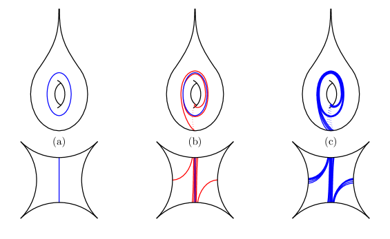
Figure 1: The three types of chain-recurrent laminations on $S_{1,1}$.

We show that the geodesic from $X$ to $Y$ is unique when $\Lambda(X,Y)$ is of type (b) or (c), and when it has type (a) the envelope has a simple, explicit description. More precisely, we have:

Theorem 1.1 (Structure of envelopes for the punctured torus).

1. For any $X,Y\in\mathcal{T}(S_{1,1})$, the envelope $E(X,Y)$ is a compact set.

2. $E(X,Y)$ varies continuously in the Hausdorff topology as a function of $X$ and $Y$.

3. If $\Lambda(X,Y)$ is not a simple closed curve, then $E(X,Y)$ is a segment on a stretch path (which is then the unique geodesic from $X$ to $Y$).

4. If $\Lambda(X,Y)=\alpha$ is a simple closed curve, then $E(X,Y)$ is a geodesic quadrilateral with $X$ and $Y$ as opposite vertices. Each edge of the quadrilateral is a stretch path along a completion of a chain-recurrent geodesic lamination properly containing $\alpha$.

In the course of proving the theorem above, we write explicit equations for the edges of the quadrilateral-type envelopes in terms of Fenchel-Nielsen coordinates (see (28)–(29)). Also note that in part (iv) of the theorem, a chain-recurrent lamination properly containing $\alpha$ has multiple completions, but they all give the same stretch path (see Corollary 2.3).

This theorem also highlights a distinction between two cases in which the $d_{\text{Th}}$-geodesic from $X$ to $Y$ is unique—the cases (b) and (c) discussed above. In case (b) the geodesic to $Y$ is unique but some initial segment of it can be chained with another stretch path and remain geodesic: The boundary of a quadrilateral-type envelope from $X$ with maximally-stretched lamination $\alpha$ furnishes an example of this. In case (c), however, a geodesic that starts along the stretch path from $X$ to $Y$ is entirely contained in that stretch path (see Proposition 5.2).

Figure 0page.1 can also be seen as an illustration of this theorem: It shows regions in $\mathcal{T}(S_{1,1})$ bounded by pairs of stretch rays from rational points on the circle at infinity to the hexagonal punctured torus. Such in-envelopes are limiting cases of the envelopes of type (iv) where $X$ is replaced by a lamination. These are defined precisely and studied in Section 5. Figure 0page.1 is discussed in more detail in Remark 5.5.

Short curves

Returning to the case of an arbitrary surface $S$ of finite type, in section 3 we establish results on the coarse geometry of Thurston metric geodesic segments. This study is similar in spirit to the one of Teichmüller geodesics in [Raf05], in that we seek to determine whether or not a simple curve $\alpha$ becomes short along a geodesic from $X$ to $Y$. As in that case, a key quantity to consider is the amount of twisting along $\alpha$ from $X$ to $Y$, denoted $d_{\alpha}(X,Y)$ and defined in Section 2.8.

For curves that interact with the maximally-stretched lamination $\Lambda(X,Y)$, meaning they belong to the lamination or intersect it essentially, we show that becoming short on a geodesic with endpoints in the thick part of $\mathcal{T}(S)$ is equivalent to the presence of large twisting:

Theorem 1.2.

There exists a constant $\epsilon_{0}$ such that the following statement holds. Let $X,Y$ lie in the $\epsilon_{0}$–thick part of $\mathcal{T}(S)$ and let $\alpha$ be a simple curve on $S$ that interacts with $\Lambda(X,Y)$. Then the minimum length $\ell_{\alpha}$ of $\alpha$ along any Thurston metric geodesic from $X$ to $Y$ satisfies

$$\frac{1}{\ell_{\alpha}}\operatorname{Log}\frac{1}{\ell_{\alpha}}\mathrel{\ooalign{\raisebox{1.4pt}{$\mkern 1.2mu\scriptstyle\ast$}\cr$\asymp$\cr\raisebox{-10.0pt}{$\mkern 0.2mu\scriptscriptstyle+$}\cr}}d_{\alpha}(X,Y)$$

with implicit constants that depend only $\epsilon_{0}$, and where $\operatorname{Log}(x)=\max(1,\log(x))$.

Here $\mathrel{\ooalign{\raisebox{1.4pt}{$\mkern 1.2mu\scriptstyle\ast$}\cr$\asymp$\cr\raisebox{-10.0pt}{$\mkern 0.2mu\scriptscriptstyle+$}\cr}}$ means equality up to an additive and multiplicative constant; see Section 2.1. The theorem above and additional results concerning length functions along geodesic segments are combined in Theorem 3.1.

In Section 4 we specialize once again to the Teichmüller space of the punctured torus in order to say more about the coarse geometry of Thurston geodesics. Here every simple curve interacts with every lamination, so Theorem 1.2 is a complete characterization of short curves in this case. Furthermore, in this case we can determine the order in which the curves become short.

To state the result, we recall that the pair of points $X,Y\in\mathcal{T}(S_{1,1})$ determine a geodesic in the dual tree of the Farey tesselation of $\mathbf{H}^{2}\simeq\mathcal{T}(S_{1,1})$. Furthermore, this path distinguishes an ordered sequence of simple curves—the pivots—and each pivot has an associated coefficient. These notions are discussed further in Section 4.

We show that pivots for $X,Y$ and short curves on a $d_{\text{Th}}$-geodesic from $X$ to $Y$ coarsely coincide in an order-preserving way, once again assuming that $X$ and $Y$ are thick:

Theorem 1.3.

Let $X,Y\in\mathcal{T}(S_{1,1})$ lie in the thick part, and let $\mathcal{G}\colon\,I\to\mathcal{T}(S_{1,1})$ be a geodesic of $d_{\text{Th}}$ from $X$ to $Y$. Let $\ell_{\alpha}$ denote the minimum of $\ell_{\alpha}(\mathcal{G}(t))$ for $t\in I$. We have:

1. If $\alpha$ is short somewhere in $\mathcal{G}$, then $\alpha$ is a pivot.

2. If $\alpha$ is a pivot with large coefficient, then $\alpha$ becomes short somewhere in $\mathcal{G}$.

3. If both $\alpha$ and $\beta$ become short in $\mathcal{G}$, then they do so in disjoint intervals whose ordering in $I$ agrees with that of $\alpha,\beta$ in $\operatorname{Pivot}(X,Y)$.

4. There is an a priori upper bound on $\ell_{\alpha}$ for $\alpha\in\operatorname{Pivot}(X,Y)$.

In this statement, various constants have been suppressed (such as those required to make short and large precise). We show that all of the constants can be taken to be independent of $X$ and $Y$, and the full statement with these constants is given as Theorem 4.3 below.

We have already seen that there may be many Thurston geodesics from $X$ to $Y$, and due to the asymmetry of the metric, reversing parameterization of a geodesic from $X$ to $Y$ does not give a geodesic from $Y$ to $X$. On the other hand, the notion of a pivot is symmetric in $X$ and $Y$. Therefore, by comparing the pivots to the short curves of an arbitrary Thurston geodesic, Theorem 4.3 establishes a kind of symmetry and uniqueness for the combinatorics of Thurston geodesic segments, despite the failure of symmetry or uniqueness for the geodesics themselves.

Rigidity

A Finsler metric on $\mathcal{T}(S)$ gives each tangent space $T_{X}\mathcal{T}(S)$ the structure of a normed vector space. Royden showed that for the Teichmüller metric, this normed vector space uniquely determines $X$ up to the action of the mapping class group [Roy71]. That is, the tangent spaces are isometric (by a linear map) if and only if the hyperbolic surfaces are isometric.

We establish the corresponding result for the Thurston’s metric on $\mathcal{T}(S_{1,1})$ and its corresponding norm $\left\|{{\mathchoice{\mkern 1.0mu\mbox{\raise 2.2pt\hbox{$\centerdot$}}\mkern 1.0mu}{\mkern 1.0mu\mbox{\raise 2.2pt\hbox{$\centerdot$}}\mkern 1.0mu}{\mkern 1.5mu\centerdot\mkern 1.5mu}{\mkern 1.5mu\centerdot\mkern 1.5mu}}}\right\|_{\mathrm{Th}}$ (the Thurston norm) on the tangent bundle.

Theorem 1.4.

Let $X,Y\in\mathcal{T}(S_{1,1})$. Then there exists an isometry of normed vector spaces

$$(T_{X}\mathcal{T}(S_{1,1}),\left\|{{\mathchoice{\mkern 1.0mu\mbox{\raise 2.2pt\hbox{$\centerdot$}}\mkern 1.0mu}{\mkern 1.0mu\mbox{\raise 2.2pt\hbox{$\centerdot$}}\mkern 1.0mu}{\mkern 1.5mu\centerdot\mkern 1.5mu}{\mkern 1.5mu\centerdot\mkern 1.5mu}}}\right\|_{\mathrm{Th}})\to(T_{Y}\mathcal{T}(S_{1,1}),\left\|{{\mathchoice{\mkern 1.0mu\mbox{\raise 2.2pt\hbox{$\centerdot$}}\mkern 1.0mu}{\mkern 1.0mu\mbox{\raise 2.2pt\hbox{$\centerdot$}}\mkern 1.0mu}{\mkern 1.5mu\centerdot\mkern 1.5mu}{\mkern 1.5mu\centerdot\mkern 1.5mu}}}\right\|_{\mathrm{Th}})$$

if and only if $X$ and $Y$ are in the same orbit of the extended mapping class group.

The idea of the proof is to recognize lengths and intersection numbers of curves on $X$ from features of the unit sphere in $T_{X}\mathcal{T}(S)$. Analogous estimates for the shape of the cone of lengthening deformations of a hyperbolic one-holed torus were established in [Gué15]. In fact, Theorem 1.4 was known to Guéritaud and can be derived from those estimates [Gué16]. We present a self-contained argument that does not use Guéritaud’s results directly, though [Gué15, Section 5.1] provided inspiration for our approach to the infinitesimal rigidity statement.

A local rigidity theorem can be deduced from the infinitesimal one, much as Royden did in [Roy71].

Theorem 1.5.

Let $U$ be a connected open set in $\mathcal{T}(S_{1,1})$, considered as a metric space with the restriction of $d_{\text{Th}}$. Then any isometric embedding $(U,d_{\text{Th}})\to(\mathcal{T}(S_{1,1}),d_{\text{Th}})$ is the restriction to $U$ of an element of the extended mapping class group.

Intuitively, this says that the quotient of $\mathcal{T}(S_{1,1})$ by the mapping class group is “totally unsymmetric”; each ball fits into the space isometrically in only one place. Of course, applying Theorem 1.5 to $U=\mathcal{T}(S_{1,1})$ we have the immediate corollary

Corollary 1.6.

Every isometry of $(\mathcal{T}(S_{1,1}),d_{\text{Th}})$ is induced by an element of the extended mapping class group, hence the isometry group is isomorphic to $\operatorname{PGL}(2,\mathbf{Z})$.

Here we have used the usual identification of the mapping class group of $S_{1,1}$ with $\operatorname{GL}(2,\mathbf{Z})$, whose action on $\mathcal{T}(S_{1,1})$ factors through the quotient $\operatorname{PGL}(2,\mathbf{Z})$.

The analogue of Corollary 1.6 for Thurston’s metric on higher-dimensional Teichmüller spaces was established by Walsh in [Wal14] using a characterization of the horofunction compactification of $\mathcal{T}(S)$. Walsh’s argument does not apply to the punctured torus, however, because it relies on Ivanov’s characterization (in [Iva97]) of the automorphism group of the curve complex (a result which does not hold for the punctured torus).

Passing from the infinitesimal (i.e. norm) rigidity to local or global statements requires some preliminary study of the smoothness of the Thurston norm. In Section 6.1 we show that the norm is locally Lipschitz continuous on $T\mathcal{T}(S)$ for any finite type hyperbolic surface $S$. By a recent result of Matveev-Troyanov [MT17], it follows that any $d_{\text{Th}}$-preserving map is differentiable with norm-preserving derivative. This enables the key step in the proof of Theorem 1.5, where Theorem 1.4 is applied to the derivative of the isometry.

Additional notes and references

In addition to Thurston’s paper [Thu86c], an exposition of Thurston’s metric and a survey of its properties can be found in [PT07]. Prior work on the coarse geometry of the Thurston metric on Teichmüller space and its geodesics can be found in [CR07] [LRT12] [LRT15]. The notion of the maximally-stretched lamination for a pair of hyperbolic surfaces has been generalized to higher-dimensional hyperbolic manifolds [Kas09] [GK17] and to vector fields on $\mathbf{H}^{2}$ equivariant for convex cocompact subgroups of $\operatorname{PSL}(2,\mathbf{R}$) [DGK16].

Acknowledgments

The authors thank the American Institute of Mathematics for hosting the workshop “Lipschitz metric on Teichmüller space” and the Mathematical Sciences Research Institute for hosting the semester program “Dynamics on Moduli Spaces of Geometric Structures” where some of the work reported here was completed. The authors gratefully acknowledge grant support from NSF DMS 0952869 and DMS 1709877 (DD), NSF DMS 1611758 (JT), NSERC RGPIN 435885 (KR), and from NSF DMS 1107452, 1107263, 1107367 “RNMS: GEometric structures And Representation varieties” (the GEAR Network). The authors also thank François Guéritaud for helpful conversations related to this work, and specifically for suggesting the statement of Theorem 6.8. Finally, the authors thank the anonymous referees for their careful reading of the paper and for helpful comments and corrections.

2 Background

2.1 Approximate comparisons

We use the notation $a\mathrel{\ooalign{\raisebox{1.4pt}{$\mkern 0.2mu\scriptstyle\ast$}\cr$\asymp$\cr}}b$ to mean that quantities $a$ and $b$ are equal up to a uniform multiplicative error, i.e. that there exists a positive constant $K$ such that $K^{-1}a\leqslant b\leqslant Ka$. Thus for example $a\mathrel{\ooalign{\raisebox{1.4pt}{$\mkern 0.2mu\scriptstyle\ast$}\cr$\asymp$\cr}}1$ means that $a$ is bounded above and below by positive constants. Similarly, the notation $a\mathrel{\ooalign{\raisebox{1.4pt}{$\mkern 0.2mu\scriptstyle\ast$}\cr$\prec$\cr}}b$ means that $a\leqslant Kb$ for some $K$.

The analogous relations up to additive error are $a\mathrel{\ooalign{\raisebox{1.6pt}{$\mkern 0.2mu\scriptscriptstyle+$}\cr$\asymp$\cr}}b$, meaning that there exists $C$ such that $a-C\leqslant b\leqslant a+C$, and $a\mathrel{\ooalign{\raisebox{1.6pt}{$\mkern 0.2mu\scriptscriptstyle+$}\cr$\prec$\cr}}b$ which means $a\leqslant b+C$ for some $C$. Hence $a\mathrel{\ooalign{\raisebox{1.6pt}{$\mkern 0.2mu\scriptscriptstyle+$}\cr$\asymp$\cr}}0$ means that $a$ is bounded above and below by constants.

For equality up to both multiplicative and additive error, we write $a\mathrel{\ooalign{\raisebox{1.4pt}{$\mkern 1.2mu\scriptstyle\ast$}\cr$\asymp$\cr\raisebox{-10.0pt}{$\mkern 0.2mu\scriptscriptstyle+$}\cr}}b$. That is, $a\mathrel{\ooalign{\raisebox{1.4pt}{$\mkern 1.2mu\scriptstyle\ast$}\cr$\asymp$\cr\raisebox{-10.0pt}{$\mkern 0.2mu\scriptscriptstyle+$}\cr}}b$ means that there exist constants $K,C$ such that $K^{-1}a-C\leqslant b\leqslant Ka+C$.

Unless otherwise specified, the implicit constants depend only on the topological type of the surface $S$. When the constants depend on the Riemann surface $X$, we use the notation $\mathrel{\ooalign{\raisebox{1.4pt}{$\mkern 0.2mu\scriptstyle\ast$}\cr$\asymp$\cr}}_{X}$ and $\mathrel{\ooalign{\raisebox{1.6pt}{$\mkern 0.2mu\scriptscriptstyle+$}\cr$\asymp$\cr}}_{X}$ instead.

For functions $f,g$ of a real variable $x$ we write $f\sim g$ to mean that $\lim_{x\to\infty}\frac{f(x)}{g(x)}=1$.

2.2 Surfaces, curves, and laminations

Throughout this paper $S$ denotes an oriented surface of finite type, i.e. the complement of a finite subset $P$ of the interior of $\bar{S}$, a compact oriented surface with boundary. Elements of $P$ are the punctures.

A multicurve is a closed 1-manifold on $S$ defined up to homotopy such that no connected component is homotopic to a point, a puncture, or boundary of $S$. A connected multicurve will just be called a curve. Note that with our definition, there are no curves on the two- or three-punctured sphere, so we will ignore those cases henceforth. The geometric intersection number $\operatorname{i}(\alpha,\beta)$ between two curves is the minimal number of intersections between representatives of $\alpha$ and $\beta$. If we fix a hyperbolic metric on $S$, then every (multi)curve has a unique geodesic representative, and $\operatorname{i}(\alpha,\beta)$ is just the number of intersections between the geodesic representative of $\alpha$ and the geodesic representative of $\beta$. For any curve $\alpha$ on $S$, we denote by $D_{\alpha}$ the left Dehn twist about $\alpha$.

Fix a complete hyperbolic metric of finite area on $S$, so that the boundary components (if any) are geodesic. A geodesic lamination $\lambda$ on $S$ is a closed subset which is a disjoint union of simple complete geodesics. These geodesics are called the leaves of $\lambda$. Two different hyperbolic metrics on $S$ determine canonically isomorphic spaces of geodesic laminations, so the space of geodesic laminations $\mathcal{GL}(S)$ depends only on the topology of $S$. This is a compact metric space equipped with the metric of Hausdorff distance on closed sets. The closure of the set of multicurves in $\mathcal{GL}(S)$ is the set of chain-recurrent laminations.

We will call a geodesic lamination maximal chain-recurrent if it is chain-recurrent and not properly contained in another chain-recurrent lamination. A geodesic lamination is complete if its complementary regions in $S$ are ideal triangles. Note that all chain-recurrent laminations are necessarily compactly supported. Thus, when $S$ has punctures, a chain-recurrent lamination can never be complete. For a given geodesic lamination $\lambda$, we refer to any complete lamination containing $\lambda$ as a completion (of $\lambda)$.

In the case of the punctured torus $S_{1,1}$, the maximal chain-recurrent laminations are types (b) and (c) in Figure 1. Case (b), i.e. a curve and a spiraling geodesic, will be especially important in the sequel, and so we introduce the following notation for these laminations: Given a curve $\alpha$, let $\alpha_{0}^{+}=\alpha\cup\delta$ where the geodesic $\delta$ spirals toward $\alpha$ in each direction, turning to the left as it does so. Similarly we define $\alpha^{-}_{0}$ to be the union of $\alpha$ and a spiraling leaf that turns right. (Adding a leaf that turns opposite ways on its two ends yields a non-chain-recurrent lamination.)

The motivation for this sign convention for $\alpha_{0}^{\pm}$ is that it is compatible with a common way to describe simple curves on $S_{1,1}$ in terms of slope while regarding $\alpha$ as vertical. More precisely, consider an oriented curve $\vec{\eta}$ with $\operatorname{i}(\eta,\alpha)=1$, and let $\vec{\alpha}$ denote the orientation of $\alpha$ so that the homology classes $[\vec{\eta}],[\vec{\alpha}]$ give a positive ordered basis of $H_{1}(S_{1,1})$ with respect to the orientation of $S_{1,1}$. If a simple curve $\gamma\neq\alpha$ has homology class $q[\vec{\eta}]+p[\vec{\alpha}]$ for some orientation, then $p/q\in\mathbf{Q}$ is the slope of $\gamma$ (relative to that basis). We consider $\alpha$ itself to have slope $1/0=\infty\in\mathbf{QP}^{1}$ and this exhibits a bijection between $\mathbf{QP}^{1}$ and the set of simple curves on $S_{1,1}$.

Now, a sequence of simple curves distinct from $\alpha$ whose slopes go to $+\infty$ have Hausdorff limit $\alpha_{0}^{+}$, while a sequence with slopes going to $-\infty$ has Hausdorff limit $\alpha_{0}^{-}$. Thus $\alpha_{0}^{+}$ (resp. $\alpha_{0}^{-}$) is approximated by curves of large positive (resp. negative) slope.

All of the maximal chain-recurrent laminations on $S_{1,1}$ have a single complementary region, which is a punctured bigon. Such a lamination therefore has exactly three completions, corresponding to the three ways to add leaves that cut the bigon into ideal triangles shown in Figure 2. (For more detail on classifying laminations on the punctured torus, we refer the reader to [BZ04].)

A convenient way to distinguish among the completions of a maximal chain-recurrent lamination $\lambda$ on the punctured torus is to use the hyperelliptic involution. This is an involutive orientation-preserving isometry $\iota$ that preserves every simple closed geodesic, and thus every chain-recurrent lamination. The action of $\iota$ on the complementary bigon of a maximal chain-recurrent lamination exchanges the two spikes, and therefore the only completion which is $\iota$-invariant is the one with leaves going to both spikes, i.e. type (i) in Figure 2. We call this the canonical completion of $\lambda$.

We denote the canonical completion of $\alpha_{0}^{+}$ by $\alpha^{+}$, and that of $\alpha_{0}^{-}$ by $\alpha^{-}$. Thus $\alpha^{\pm}=\alpha_{0}^{\pm}\cup w\cup w^{\prime}$ where $w$ and $w^{\prime}$ are leaves emanating from the puncture and spiraling into $\alpha$. For example, $\alpha^{+}$ is shown in Figure 3.

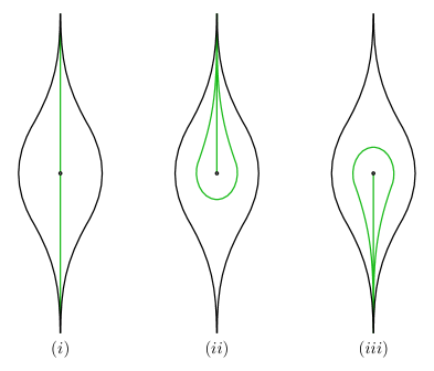
Figure 2: The three ways to complete a maximal chain-recurrent lamination on $S_{1,1}$ by adding two leaves in its complementary bigon.

The stump of a geodesic lamination (in the terminology of [Thé07]) is its maximal compactly-supported sublamination that admits a transverse measure of full support.

2.3 Teichmüller space

Let $\mathcal{T}(S)$ be the Teichmüller space of complete finite-area hyperbolic structures on $S$. We will only consider $\mathcal{T}(S)$ in cases where $S$ has no boundary. The space $\mathcal{T}(S)$ is homeomorphic to $\mathbf{R}^{6g-6+2n}$, if $S$ has genus $g$ and $n$ punctures. Given $X\in\mathcal{T}(S)$ and a curve $\alpha$ on $S$, we denote by $\ell_{\alpha}(X)$ the length of the geodesic representative of $\alpha$ on $X$. For brevity we refer to $\ell_{\alpha}(X)$ as the length of $\alpha$ on $X$.

For any $\epsilon>0$, we will denote by $\mathcal{T}_{\epsilon}(S)$ the set of points in $\mathcal{T}(S)$ on which every curve has length at least $\epsilon$; this is the $\epsilon$-thick part of Teichmüller space.

A positive real number $\epsilon$ is called a (two-dimensional) Margulis number if two distinct curves on a hyperbolic surface of length less than $\epsilon$ are necessarily disjoint. Fix a Margulis number $\epsilon_{M}<1$ such that that for any curve $\alpha$ of length less than $\epsilon_{M}$, the shortest curve $\beta$ that intersects $\alpha$ has $\operatorname{i}(\alpha,\beta)\leqslant 2$. It follows from the collar lemma that any sufficiently small $\epsilon_{M}$ has this property.

2.4 Shearing of ideal triangles

Let $\mathbf{H}$ denote the upper half plane model of the hyperbolic plane, with ideal boundary $\partial\mathbf{H}=\mathbf{R}\cup\left\{{\infty}\right\}$. In this section, we will define the shearing of two ideal triangles in $\mathbf{H}$ which share an ideal vertex. This is a specific case of the more general shearing defined in [Bon96, Section 2].

Two distinct points $x,y\in\partial\mathbf{H}$ determine a geodesic $[x,y]$ and three distinct points $x,y,z\in\partial\mathbf{H}$ determine an ideal triangle $\Delta(x,y,z)$. Recall that an ideal triangle in $\mathbf{H}$ has a unique inscribed circle which is tangent to all three sides of the triangle. Each tangency point is called the midpoint of the side.

Let $\gamma=[\gamma^{+},\gamma^{-}]$ be a geodesic in $\mathbf{H}$. Suppose two ideal triangles $\Delta$ and $\Delta^{\prime}$ lie on different sides of $\gamma$. We allow the possibility that $\gamma$ is an edge of $\Delta$ or $\Delta^{\prime}$ (or both). Suppose $\Delta$ is asymptotic to $\gamma^{+}$ and the $\Delta^{\prime}$ is asymptotic to $\gamma^{-}$. Let $m$ be the midpoint along the side of $\Delta$ closest to $\gamma$. The pair $\gamma^{+}$ and $m$ determine a horocycle that intersects $\gamma$ at a point $p$. Let $m^{\prime}$ and $p^{\prime}$ be defined similarly using $\Delta^{\prime}$ and $\gamma^{-}$. We say $p^{\prime}$ is to the left of $p$ (relative to $\Delta$ and $\Delta^{\prime}$) if the path along the horocycle from $m$ to $p$ and along $\gamma$ from $p$ and $p^{\prime}$ turns left; $p^{\prime}$ is to the right of $p$ otherwise. Note that $p^{\prime}$ is to the left of $p$ if and only if $p$ is to the left of $p^{\prime}$. The shearing $s_{\gamma}(\Delta,\Delta^{\prime})$ along $\gamma$ relative to the two triangles is the signed distance between $p$ and $p^{\prime}$, where the sign is positive if $p^{\prime}$ is to the left of $p$ and negative otherwise. Note that this sign convention gives $s_{\gamma}(\Delta,\Delta^{\prime})=s_{\gamma}(\Delta^{\prime},\Delta)$.

2.5 Shearing coordinates in Teichmüller space

Given any complete geodesic lamination $\lambda$, there is an embedding $s_{\lambda}\colon\,\mathcal{T}(S)\to\mathbf{R}^{N}$ by the shearing coordinates relative to $\lambda$, where $N=\dim\mathcal{T}(S)$. The image of this embedding is an open convex cone. Details of the construction of this embedding can be found in [Bon96] and [Thu86c, Section 9].

Using the shearing of ideal triangles discussed above, we will define the shearing coordinates in the case where $\lambda$ is the canonical completion of a maximal chain-recurrent lamination on $S_{1,1}$ with finitely many leaves. That is, we consider $\lambda=\alpha^{+}$ or $\lambda=\alpha^{-}$ for a simple curve $\alpha$, and describe the map $s_{\lambda}\colon\,\mathcal{T}(S_{1,1})\to\mathbf{R}^{2}$.

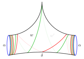
Figure 3: Leaves of $\alpha^{+}$ (the canonical completion of $\alpha_{0}^{+}$) shown in the torus cut open along $\alpha$.

We begin with an auxiliary map $s_{\lambda}^{0}:\mathcal{T}(S_{1,1})\to\mathbf{R}^{4}$ which records a shearing parameter for each leaf of $\lambda$, and then we identify the $2$-dimensional subspace of $\mathbf{R}^{4}$ that contains the image in this specific situation.

Let $l$ be a leaf of $\lambda$ and fix a lift ${\widetilde{l}}$ of $l$ to ${\widetilde{X}}=\mathbf{H}$. If $l$ is a non-compact leaf, then $l$ bounds two ideal triangles in $X$, which admit lifts $\Delta$ and $\Delta^{\prime}$ with common side ${\widetilde{l}}$. If $l=\alpha$ is the compact leaf, then we choose $\Delta$ and $\Delta^{\prime}$ to be lifts of the two ideal triangles complementary to $\lambda$ that lie on different sides of ${\widetilde{l}}$ and which are each asymptotic to one of the ideal points of ${\widetilde{l}}$. Now define $s_{l}(X)=s_{{\widetilde{l}}}(\Delta,\Delta^{\prime})$, and let the $s_{\lambda}^{0}:\mathcal{T}(S_{1,1})\to\mathbf{R}^{4}$ be the map defined by

$$s_{\lambda}^{0}(X)=(s_{\delta}(X),s_{\alpha}(X),s_{w}(X),s_{w^{\prime}}(X)).$$

We claim that in fact, $s_{w}(X)=s_{w^{\prime}}(X)=0$ and that $s_{\delta}(X)=\mp\ell_{\alpha}(X)$ for $\lambda=\alpha^{\pm}$. It will then follow that $s_{\lambda}^{0}$ takes values in a $2$-dimensional linear subspace of $\mathbf{R}^{4}$, allowing us to equivalently consider the embedding $s_{\lambda}:\mathcal{T}(S_{1,1})\to\mathbf{R}^{2}$ defined by

$$s_{\lambda}(X)=(\ell_{\alpha}(X),s_{\alpha}(X)).$$

To establish the claim, cut the surface $X$ open along $\alpha$ to obtain a pair of pants which is further decomposed by $w,w^{\prime},\delta$ into a pair of ideal triangles. The boundary lengths of this hyperbolic pair of pants are $\ell_{\alpha}$, $\ell_{\alpha}$, and $0$. Gluing a pair of ideal triangles along their edges but with their edge midpoints shifted by signed distances $a,b,c$ gives a pair of pants with boundary lengths $|a+b|,|b+c|,|a+c|$, and with the signs of $a+b,b+c,a+c$ determining the direction in which the seams spiral toward those boundary components (this is discussed in more detail in [Thu86a, Section 3.9]). Specifically, a positive sum corresponds to the seam turning to the right while approaching the corresponding boundary geodesic, and a negative sum corresponds to the seam turning to the right. Applying this to our situation, and recalling that for $\lambda=\alpha^{+}$ all spiraling leaves turn left when approaching the boundary of the pair of pants, and we obtain

$$s_{w}(X)+s_{\delta}(X)=s_{w^{\prime}}(X)+s_{\delta}(X)=-\ell_{\alpha}$$

and

$$s_{w}(X)+s_{w^{\prime}}(X)=0.$$

This gives $s_{w}(X)=s_{w^{\prime}}(X)=0$ and $s_{\delta}(X)=-\ell_{\alpha}(X)$. For the case $\lambda=\alpha^{-}$ the equations are the same except that $-\ell_{\alpha}$ is replaced by $\ell_{\alpha}$, and the solution becomes $s_{w}(X)=s_{w^{\prime}}(X)=0$ and $s_{\delta}(X)=\ell_{\alpha}$.

Finally, we consider the effect of the various choices made in the construction of $s_{\lambda}(X)$. The coordinate $\ell_{\alpha}(X)$ is of course canonically associated to $X$, and independent of any choices. For $s_{\alpha}(X)$, however, we had to choose a pair of triangles $\Delta,\Delta^{\prime}$ on either side of the lift $\tilde{\alpha}$. In this case, different choices differ by finitely many moves in which one of the triangles is replaced by a neighbor on the other side of a lift of $w$, $w^{\prime}$, or $\delta$. Each such move changes the value of $s_{\alpha}(X)$ by adding or subtracting one of the values $s_{w}(X)$, $s_{w^{\prime}}(X)$, or $s_{\delta}(X)$; this is the additivity of the shearing cocycle established in [Bon96, Section 2]. By the computation above each of these moves actually adds $0$ or $\pm\ell_{\alpha}(X)$. Hence $s_{\alpha}(X)$ is uniquely determined up to addition of an integer multiple of $\ell_{\alpha}(X)$.

2.6 The Thurston metric

For a pair of points $X,Y\in\mathcal{T}(S)$, in the introduction we defined the quantity

$$d_{\text{Th}}(X,Y)=\sup_{\alpha}\log\frac{\ell_{\alpha}(Y)}{\ell_{\alpha}(X)}$$

where the supremum is taken over all simple curves. Another measure of the difference of hyperbolic structures, in some ways dual to this length ratio, is

$$L(X,Y)=\inf_{f}\log L_{f}$$

where $L_{f}$ is the Lipschitz constant, and where the infimum is taken over Lipschitz maps $f:X\to Y$ in the preferred homotopy class. Thurston showed:

Theorem 2.1.

For all $X,Y\in\mathcal{T}(S))$ we have $d_{\text{Th}}(X,Y)=L(X,Y)$, and this function is an asymmetric metric, i.e. it is positive unless $X=Y$ and it obeys the triangle inequality.

Denote by $\overline{d}_{\text{Th}}(X,Y)=\max\left\{{d_{\text{Th}}(X,Y),d_{\text{Th}}(Y,X)}\right\}$. The topology of $\mathcal{T}(S)$ is compatible with $\overline{d}_{\text{Th}}$, so by $X_{i}\to X$ we will mean $\overline{d}_{\text{Th}}(X_{i},X)\to 0$. By the Hausdorff distance on closed sets in $\mathcal{T}(S)$ we will mean with respect to the metric $\overline{d}_{\text{Th}}$.

Thurston showed that the infimum Lipschitz constant is realized by a homeomorphism from $X$ to $Y$. Any map which realizes the infimum is called optimal.

Further, Thurston constructs a chain-recurrent lamination $\Lambda(X,Y)$ such that there exists a $e^{d_{\text{Th}}(X,Y)}$-Lipschitz map in the preferred homotopy class from a neighborhood of $\Lambda(X,Y)$ in $X$ to an neighborhood of the same lamination in $Y$, multiplying arc length along $\Lambda(X,Y)$ by a factor of $e^{d_{\text{Th}}(X,Y)}$, and so that $\Lambda(X,Y)$ is the largest chain-recurrent lamination with this property. We call $\Lambda(X,Y)$ the maximally-stretched lamination (from $X$ to $Y$). The same lamination is also characterized in terms of optimal maps: $\Lambda(X,Y)$ is the largest chain-recurrent lamination such that every optimal map from $X$ to $Y$ multiplies arc length on $\Lambda(X,Y)$ by a factor of $e^{d_{\text{Th}}(X,Y)}$.

The length ratio for simple curves extends continuously to $\mathcal{PML}(S)$, which is compact. Therefore, the length-ratio supremum is always realized by some measured lamination. Any measured lamination that realizes the supremum has support contained in the stump of $\Lambda(X,Y)$.

Suppose a parameterized path $\mathcal{G}\colon\,[0,d]\to\mathcal{T}(S)$ is a geodesic from $X$ to $Y$ (parameterized by unit speed). Then the following holds: for any $s,t\in[0,d]$ with $s<t$ and for any arc $\omega$ contained in the geometric realization of $\Lambda(X,Y)$ on $X$, the arc length of $\omega$ is stretched by a factor of $e^{t-s}$ under an optimal map from $\mathcal{G}(s)$ to $\mathcal{G}(t)$. We will sometimes denote $\Lambda(X,Y)$ by $\lambda_{\mathcal{G}}$.

2.7 Stretch paths

Certain geodesics of Thurston’s metric can be described using shearing coordinates. Let $\lambda$ be a complete geodesic lamination and $X\in\mathcal{T}(S)$. For any $t\in\mathbf{R}$ let $\operatorname{stretch}(X,\lambda,t)$ be the unique point in $\mathcal{T}(S)$ such that

$$s_{\lambda}(\operatorname{stretch}(X,\lambda,t))=e^{t}s_{\lambda}(X).$$

Letting $t$ vary, we have that $\operatorname{stretch}(X,\lambda,t)$ is a parameterized path in $\mathcal{T}(S)$ that maps to an open ray from the origin in $\mathbf{R}^{N}$ under the shearing coordinates. This is the stretch path along $\lambda$ from $X$.

Thurston showed that the path $t\mapsto\operatorname{stretch}(X,\lambda,t)$ is a geodesic in $\mathcal{T}(S)$ in the sense of (2). Note that we always consider the stretch path to be oriented in the direction of increasing $t$, which is natural since the asymmetry of the metric implies that the same path parameterized in the opposite direction may not be geodesic.

Also, if $\lambda_{0}\subset\lambda$ is the largest chain-recurrent sublamination, then $\lambda_{0}$ is the maximally-stretched lamination for any pair of points $\operatorname{stretch}(X,\lambda,s)$ and $\operatorname{stretch}(X,\lambda,t)$ with $s<t$.

Removing the point $X$ from a stretch path from $X$ leaves two (open) stretch rays; of these, the one corresponding to $t>0$ is a stretch ray starting at $X$ and that with $t<0$ is the one ending at $X$.

Thurston used stretch paths to show that $\mathcal{T}(S)$ equipped with the Thurston metric is a geodesic metric space. We summarize his results below. See the statement and proof of [Thu86c, Theorem 8.5]) for more details.

Theorem 2.2 ([Thu86c]).

For any $X,Y\in\mathcal{T}(S)$, let $\Lambda(X,Y)$ be the maximally-stretched lamination from $X$ to $Y$. Let $\lambda$ be any completion of $\Lambda(X,Y)$. Then there exists a geodesic $\mathcal{G}$ from $X$ to $Y$ consisting of a finite concatenation of stretch path segments

$$\mathcal{G}=\mathcal{G}_{1}\cdots\mathcal{G}_{n},$$

where $\mathcal{G}_{1}$ is a segment of $\operatorname{stretch}(X,\lambda,t)$, and all other $\mathcal{G}_{i}$’s stretch along some complete lamination containing $\Lambda(X,Y)$. Furthermore, such a geodesic can be chosen so that if $X_{i}$ is the initial point of $\mathcal{G}_{i}$, then for all $i>1$ we have $\Lambda(X_{i},Y)\supsetneq\Lambda(X_{i-1},Y)$. In particular, we can always take $n\leqslant 2|\chi(S)|$.

In general, geodesics of the Thurston metric from $X$ to $Y$ are not unique. But when $\Lambda(X,Y)$ is maximal chain-recurrent, then there is a unique geodesic. This statement follows from Theorem 2.2 but it is not explicitly stated in [Thu86c]. For completeness, we provide a proof:

Corollary 2.3.

Given $X,Y\in\mathcal{T}(S)$, suppose $\Lambda(X,Y)$ is maximal chain-recurrent. Let $\lambda$ be a completion of $\Lambda(X,Y)$. Then $\operatorname{stretch}(X,\lambda,t)$ is the unique geodesic from $X$ to $Y$. In particular, for the punctured torus $S_{1,1}$, the three completions of $\Lambda(X,Y)$ give rise to the same stretch path in $\mathcal{T}(S_{1,1})$.

Proof.

We first show that the stretch path for $\lambda$ connects $X$ to $Y$, i.e. $\operatorname{stretch}(X,\lambda,t)=Y$ for some $t$. By Theorem 2.2, there is a geodesic path $\mathcal{G}$ from $X$ to $Y$ consisting of a concatenation of segments along stretch paths $\mathcal{G}_{1},\ldots,\mathcal{G}_{n}$, where $\mathcal{G}_{1}$ is a segment of $\{\operatorname{stretch}(X,\lambda,t)\>\colon\>t\geqslant 0\}$. Let $X_{i}$ be the initial point of $\mathcal{G}_{i}$. If $n\geqslant 2$, then $\Lambda(X,Y)=\Lambda(X_{1},Y)\subsetneq\Lambda(X_{2},Y)$ by Theorem 2.2. But this is impossible since $\Lambda(X,Y)$ is maximal chain-recurrent, so $n=1$ and $Y$ lies on $\cal G_{1}$.

Now suppose $\cal G$ is any geodesic from $X$ to $Y$. Let $Z$ be a point on $\cal G$. We have $\Lambda(X,Y)\subset\Lambda(X,Z)$. Since $\Lambda(X,Y)$ is maximal chain-recurrent, $\Lambda(X,Z)=\Lambda(X,Y)$. By the previous discussion, we can connect $X$ to $Z$ by a segment of $\operatorname{stretch}(X,\lambda,t)$. Since this true for all $Z$ in $\mathcal{G}$, the geodesic $\mathcal{G}$ must be a segment of $\operatorname{stretch}(X,\lambda,t)$. ∎

2.8 Twisting

There are several notions of twisting which we will define below. While these notions are defined for different classes of objects, in cases where several of the definitions apply, they are equal up to an additive constant.

Let $A$ be an annulus. Fix an orientation of the core curve $\alpha$ of $A$. For any simple arc $\omega$ in $A$ with endpoints on different components of $\partial A$, we orient $\omega$ so that the algebraic intersection number $\omega\cdot\alpha$ is equal to one. Given an ordered pair of simple arcs $\omega$ and $\omega^{\prime}$, the choice of the orientation above allows us to assign a sign to each intersection point in the interior of $A$ between $\omega$ and $\omega^{\prime}$. The sum $\omega\cdot\omega^{\prime}$ of these signed intersections is called the algebraic intersection number between $\omega$ and $\omega^{\prime}$. Note that $\omega\cdot\omega^{\prime}$ is independent of the choice of the orientation of $\alpha$. Also note that we do not consider intersections between $\omega$ and $\omega^{\prime}$ in the boundary of $A$. With our choice, we always have $\omega\cdot D_{\alpha}(\omega)=1$, where as above $D_{\alpha}$ denotes the left Dehn twist about $\alpha$.

Now let $S$ be a surface and $\alpha$ is a simple closed curve on $S$. Let $\widehat{S}\to S$ be the covering space associated to $\pi_{1}(\alpha)<\pi_{1}(S)$. Then $\widehat{S}$ has a natural Gromov compactification that is homeomorphic to a closed annulus. By construction, the core curve $\widehat{\alpha}$ of this annulus maps homeomorphically to $\alpha$ under this covering map.

Let $\lambda$ and $\lambda^{\prime}$ be two geodesic laminations (possibly curves) on $S$, both intersecting $\alpha$ transversely. We define their (signed) twisting relative to $\alpha$ as $\operatorname{twist}_{\alpha}(\lambda,\lambda^{\prime})=\min{\widehat{\omega}\cdot\widehat{\omega}^{\prime}}$, where $\widehat{\omega}$ is a lift of a leaf of $\lambda$ and $\widehat{\omega^{\prime}}$ is a lift of a leaf of $\lambda^{\prime}$, with both lifts intersecting $\widehat{\alpha}$, and the minimum is taken over all such leaves and their lifts. Note that for any two such lifts $\omega$ and $\omega^{\prime}$ (still intersecting $\widehat{\alpha}$) the quantity $\widehat{\omega}\cdot\widehat{\omega}^{\prime}$ exceeds $\operatorname{twist}_{\alpha}(\lambda,\lambda^{\prime})$ by at most $2$.

Next we define the twisting of two hyperbolic metrics $X$ and $Y$ on $S$ relative to $\alpha$. Let $\widehat{X},\widehat{Y}$ denote the lifts of these hyperbolic structures to $\widehat{S}$. Using the hyperbolic structure $\widehat{X}$, choose a geodesic $\widehat{\omega}$ that is orthogonal to the geodesic in the homotopy class of $\widehat{\alpha}$. Let $\widehat{\omega}^{\prime}$ be a geodesic constructed similarly from $\widehat{Y}$. We set $\operatorname{twist}_{\alpha}(X,Y)=\min\widehat{\omega}\cdot\widehat{\omega}^{\prime}$, where the minimum is taken over all possible choices for $\widehat{\omega}$ and $\widehat{\omega}^{\prime}$. Similar to the previous case, this minimum differs from the intersection number $\widehat{\omega}\cdot\widehat{\omega}^{\prime}$ for a particular pair of choices by at most $2$.

Finally, we define $\operatorname{twist}_{\alpha}(X,\lambda)$, the twisting of a lamination $\lambda$ about a curve $\alpha$ on $X$. This is defined if $\lambda$ contains a leaf that intersects $\alpha$ transversely. Let $\widehat{\omega}$ be a geodesic of $\widehat{X}$ orthogonal to the geodesic homotopic to $\widehat{\alpha}$. Let $\omega^{\prime}$ be any leaf of $\lambda$ intersecting $\alpha$, and let $\widehat{\omega}^{\prime}$ be a lift of this leaf to $\widehat{X}$ which intersects $\widehat{\alpha}$. Then $\operatorname{twist}_{\alpha}(X,\lambda)=\min{\widehat{\omega}\cdot\widehat{\omega}^{\prime}}$, with the minimum taken over all choices of $\omega^{\prime}$, $\widehat{\omega}^{\prime}$, and $\widehat{\omega}$.

Each type of twisting defined above is signed. In some cases the absolute value of the twisting is the relevant quantity; we use the notation $d_{\alpha}({\mathchoice{\mkern 1.0mu\mbox{\raise 2.2pt\hbox{$\centerdot$}}\mkern 1.0mu}{\mkern 1.0mu\mbox{\raise 2.2pt\hbox{$\centerdot$}}\mkern 1.0mu}{\mkern 1.5mu\centerdot\mkern 1.5mu}{\mkern 1.5mu\centerdot\mkern 1.5mu}},{\mathchoice{\mkern 1.0mu\mbox{\raise 2.2pt\hbox{$\centerdot$}}\mkern 1.0mu}{\mkern 1.0mu\mbox{\raise 2.2pt\hbox{$\centerdot$}}\mkern 1.0mu}{\mkern 1.5mu\centerdot\mkern 1.5mu}{\mkern 1.5mu\centerdot\mkern 1.5mu}})=\left|{\operatorname{twist}_{\alpha}({\mathchoice{\mkern 1.0mu\mbox{\raise 2.2pt\hbox{$\centerdot$}}\mkern 1.0mu}{\mkern 1.0mu\mbox{\raise 2.2pt\hbox{$\centerdot$}}\mkern 1.0mu}{\mkern 1.5mu\centerdot\mkern 1.5mu}{\mkern 1.5mu\centerdot\mkern 1.5mu}},{\mathchoice{\mkern 1.0mu\mbox{\raise 2.2pt\hbox{$\centerdot$}}\mkern 1.0mu}{\mkern 1.0mu\mbox{\raise 2.2pt\hbox{$\centerdot$}}\mkern 1.0mu}{\mkern 1.5mu\centerdot\mkern 1.5mu}{\mkern 1.5mu\centerdot\mkern 1.5mu}})}\right|$ for the corresponding unsigned twisting in each case.

The following way to compute the unsigned twisting $d_{\alpha}(X,\lambda)=\left|{\operatorname{twist}_{\alpha}(X,\lambda)}\right|$ will be useful in the sequel. Consider the universal cover ${\widetilde{X}}\mathrel{\cong}\mathbf{H}$. Let ${\widetilde{\alpha}}$ be a lift of $\alpha$ and let ${\widetilde{\omega}}^{\prime}$ be a lift of a leaf of $\lambda$ intersecting ${\widetilde{\alpha}}$. Let $L$ be the length of the orthogonal projection of ${\widetilde{\omega}}^{\prime}$ to ${\widetilde{\alpha}}$ and let $\ell$ be the length of the geodesic representative of $\alpha$ on $X$. Let ${\widetilde{\omega}}$ be an orthogonal geodesic of ${\widetilde{\alpha}}$. There is a loxodromic isometry $T$ of $\mathbf{H}$ associated to $\alpha$ that preserves ${\widetilde{\alpha}}$, and applying powers of this isometry to ${\widetilde{\omega}}$ gives a family of orthogonal geodesics to ${\widetilde{\alpha}}$ which meet it at points spaced by distance $\ell$. Then $d_{\alpha}(X,\lambda)$ is the number of these translates that intersect ${\widetilde{\omega}}^{\prime}$, as each such translate gives one intersection in the quotient $\widehat{X}=\mathbf{H}/\langle T\rangle$ considered above. Therefore, this number is between $(\lfloor L/\ell\rfloor-1)$ and $\lfloor L/\ell\rfloor$, and $d_{\alpha}(X,\lambda)\mathrel{\ooalign{\raisebox{1.6pt}{$\mkern 0.2mu\scriptscriptstyle+$}\cr$\asymp$\cr}}L/\ell$ with additive error at most $2$ (see also [Min96, Section 3] for more details).

3 Twisting parameter along a Thurston geodesic

In this section, $S$ is any oriented surface of finite type and $\mathcal{T}(S)$ is the associated Teichmüller space.

Recall that $\mathcal{T}_{\epsilon}(S)$ denotes the $\epsilon$-thick part of $\mathcal{T}(S)$. Consider two points $X,Y\in\mathcal{T}_{\epsilon}(S)$. Recall that we say a curve $\alpha$ interacts with a geodesic lamination $\lambda$ if $\alpha$ is a leaf of $\lambda$ or if $\alpha$ intersects $\lambda$ essentially. Suppose $\alpha$ is a curve that interacts with $\Lambda(X,Y)$. Let $\mathcal{G}\colon\,[0,T]\to\mathcal{T}$ be any geodesic from $X$ to $Y$, and let $\ell_{\alpha}=\min_{t}\ell_{\alpha}(t)$. We are interested in curves which become short somewhere along $\mathcal{G}$. We call an interval of time $[a,b]\subset[0,T]$ the active interval for $\alpha$ along $\mathcal{G}$ if $[a,b]$ is the maximal such interval with $\ell_{\alpha}(a)=\ell_{\alpha}(b)=\epsilon$. Note that any curve which is sufficiently short somewhere on $\mathcal{G}$ has a nontrivial active interval.

The main goal of this section is to prove the following theorem, which in particular establishes Theorem 1.2. As in the introduction we use the notation $\operatorname{Log}(x)=\min(1,\log(x))$. Denote $X_{t}=\mathcal{G}(t)$.

Theorem 3.1.

There exists a constant $\epsilon_{0}$ such that the following statement holds. Let $X,Y\in\mathcal{T}_{\epsilon_{0}}(S)$ and $\alpha$ be a curve that interacts with $\Lambda(X,Y)$. Let $\mathcal{G}$ be any geodesic from $X$ to $Y$ and $\ell_{\alpha}=\min_{t}\ell_{\alpha}(t)$. Then

$$d_{\alpha}(X,Y)\mathrel{\ooalign{\raisebox{1.4pt}{$\mkern 1.2mu\scriptstyle\ast$}\cr$\asymp$\cr\raisebox{-10.0pt}{$\mkern 0.2mu\scriptscriptstyle+$}\cr}}\frac{1}{\ell_{\alpha}}\operatorname{Log}\frac{1}{\ell_{\alpha}}.$$

If $\ell_{\alpha}<\epsilon_{0}$, then $d_{\alpha}(X,Y)\mathrel{\ooalign{\raisebox{1.6pt}{$\mkern 0.2mu\scriptscriptstyle+$}\cr$\asymp$\cr}}d_{\alpha}(X_{a},X_{b})$, where $[a,b]$ is the active interval for $\alpha$. Further, for all sufficiently small $\ell_{\alpha}$, the twisting $d_{\alpha}(X_{t},\lambda)$ is uniformly bounded for all $t\leqslant a$ and $\ell_{\alpha}(t)\mathrel{\ooalign{\raisebox{1.4pt}{$\mkern 0.2mu\scriptstyle\ast$}\cr$\asymp$\cr}}e^{t-b}\ell_{\alpha}(b)$ for all $t\geqslant b$. All errors in this statement depend only on $\epsilon_{0}$.

Note that if $\alpha$ is a leaf of $\Lambda(X,Y)$, then it does not have an active interval because its length grows exponentially along $\mathcal{G}$, and the theorem above says that in this $d_{\alpha}(X,Y)$ is uniformly bounded. If $\alpha$ crosses a leaf of $\Lambda(X,Y)$, then $d_{\alpha}(X,Y)$ is large if and only if $\alpha$ gets short along any geodesic from $X$ to $Y$. Moreover, the minimum length of $\alpha$ is the same for any geodesic from $X$ to $Y$, up to a multiplicative constant. Further, the theorem says that, essentially, all of the twisting about $\alpha$ occurs in the active interval $[a,b]$ of $\alpha$.

Before proceeding to the proof of the theorem, we need to introduce a notion of horizontal and vertical components for a curve that crosses a leaf of $\Lambda(X,Y)$ and analyze how their lengths change in the active interval. This analysis will require some lemmas from hyperbolic geometry.

Lemma 3.2.

Let $\omega$ and $\omega^{\prime}$ be two disjoint geodesics in $\mathbf{H}$ with no endpoint in common. Let $p\in\omega$ and $p^{\prime}\in\omega^{\prime}$ be the endpoints of the common perpendicular between $\omega$ and $\omega^{\prime}$. Let $x\in\omega$ be arbitrary and let $x^{\prime}\in\omega^{\prime}$ be the point on the same side of $[p,p^{\prime}]$ as $x$ such that $d_{\mathbf{H}}(x,p)=d_{\mathbf{H}}(x^{\prime},p^{\prime})$. Then

$$\sinh\frac{d_{\mathbf{H}}(p,p^{\prime})}{2}\cosh d_{\mathbf{H}}(x,p)=\sinh\frac{d_{\mathbf{H}}(x,x^{\prime})}{2}.$$ (3)

For any $y\in\omega^{\prime}$, we have

$$\sinh d_{\mathbf{H}}(p,p^{\prime})\cosh d_{\mathbf{H}}(x,p)\leqslant\sinh d_{\mathbf{H}}(x,y)$$ (4)

and

$$d_{\mathbf{H}}(x^{\prime},y)\leqslant d_{\mathbf{H}}(x,y).$$ (5)

Figure 4: Saccheri and Lambert quadrilaterals.

Proof.

We refer to Figure 4 for the proof. Equation (3) is well known, as the four points $x,x^{\prime},p^{\prime},p$ form a Saccheri quadrilateral. The point $y^{\prime}\in\omega^{\prime}$ closest to $x$ has $\angle xy^{\prime}p^{\prime}=\pi/2$, so $x,y^{\prime},p^{\prime},p$ forms a Lambert quadrilateral and the following identity holds

$$\sinh d_{\mathbf{H}}(p,p^{\prime})\cosh d_{\mathbf{H}}(x,p)=\sinh d_{\mathbf{H}}(x,y^{\prime})\\$$

Equation (4) follows since $d_{\mathbf{H}}(x,y^{\prime})\leqslant d_{\mathbf{H}}(x,y)$. For (5), set $A=\angle xx^{\prime}y$ and $B=\angle x^{\prime}xy$ and consider the triangle $\triangle xx^{\prime}y$. Depending on which side of $x^{\prime}$ the point $y$ is, $A$ is obtuse or acute. In any case, $A\geqslant B$. It is a standard fact that the side opposite the bigger angle in a triangle is longer. Hence $d_{\mathbf{H}}(x,y)\geqslant d_{\mathbf{H}}(x^{\prime},y)$. ∎

In this section we will often use the following elementary estimates for hyperbolic trigonometric functions. The proofs are omitted.

Lemma 3.3.

1. If $0\leqslant x\leqslant 1$ or $0\leqslant\sinh(x)\leqslant 1$, we have $\sinh(x)\leqslant 2x$.

2. For all $x\geqslant 0$, $\frac{1}{2}e^{x}\leqslant\cosh(x)\leqslant e^{x}$ and $x\leqslant\sinh(x)\leqslant\frac{1}{2}e^{x}$.

3. For all $x\geqslant 1$, we have $\sinh(x)\geqslant\frac{1}{4}e^{x}$.

4. For all $x\geqslant 1$, we have

   $$\log(2)\leqslant\operatorname{arcsinh}(x)-\log(x)\leqslant\log(3)$$

   and

   $$0\leqslant\operatorname{arccosh}(x)-\log(x)\leqslant\log(2).$$

Now consider $X\in\mathcal{T}(S)$ and a geodesic lamination $\lambda$ on $X$. If $\alpha$ crosses a leaf $\omega$ of $\lambda$, define $V_{X}(\omega,\alpha)$ to be a shortest arc with endpoints on $\omega$ that, together with an arc $H_{X}(\omega,\alpha)$ of $\omega$, form a curve homotopic to $\alpha$. Thus $V_{X}(\omega,\alpha)$ and $H_{X}(\omega,\alpha)$ meet orthogonally and $\alpha$ passes through the midpoints of both of these arcs (see Figure 5). If $\alpha$ is a leaf of $\lambda$, then we set $H_{X}(\omega,\alpha)=\alpha$ and let $V_{X}(\omega,\alpha)$ be the empty set.

Define $h_{X}$ and $v_{X}$ to be the lengths of $H_{X}(\omega,\alpha)$ and $V_{X}(\omega,\alpha)$ respectively. By considering the right triangles formed by these curves and $\alpha$ (which have hypotenuse along $\alpha$), it is immediate that

$$\max(h_{X},v_{X})\leqslant\ell_{\alpha}(X)\leqslant h_{X}+v_{X}.$$ (6)

The quantities $h_{X}$ and $v_{X}$ can be computed in the universal cover ${\widetilde{X}}\cong\mathbf{H}$ as follows. Let ${\widetilde{\omega}}$ and ${\widetilde{\alpha}}$ be intersecting lifts of $\omega$ and $\alpha$ to $\mathbf{H}$. Let $\phi$ be the hyperbolic isometry with axis ${\widetilde{\alpha}}$ and translation length $\ell_{\alpha}(X)$. Set ${\widetilde{\omega}}^{\prime}=\phi({\widetilde{\omega}})$ and let $\psi$ be the hyperbolic isometry taking ${\widetilde{\omega}}$ to ${\widetilde{\omega}}^{\prime}$ with axis perpendicular to the two geodesics. Since $\phi$ and $\psi$ both take $\omega$ to $\omega^{\prime}$, their composition $\psi^{-1}\phi$ is a hyperbolic isometry with axis ${\widetilde{\omega}}$. The quantity $v_{X}$ is the translation length of $\psi$ and $h_{X}$ is the translation length of $\psi^{-1}\phi$. For the latter, this means that $h_{X}=d_{\mathbf{H}}(\psi(q),\phi(q))$ for any $q\in{\widetilde{\omega}}$.

In the following, let $X_{t}=\mathcal{G}(t)$ be a geodesic segment and let $\lambda=\lambda_{\mathcal{G}}$. Let $\alpha$ be a curve that interacts with $\lambda$. We will refer to $V_{X_{t}}(\omega,\alpha)$ and $H_{X_{t}}(\omega,\alpha)$ as the vertical and horizontal components of $\alpha$ at $X_{t}$. We are interested in the lengths $h_{t}=h_{X_{t}}$ and $v_{t}=v_{X_{t}}$ of the horizontal and vertical components of $\alpha$ as functions of $t$. We will show that $v_{t}$ decreases super-exponentially, while $h_{t}$ grows exponentially. These statements are trivial if $\alpha$ is a leaf of $\lambda$, so we will always assume that $\alpha$ crosses a leaf $\omega$ of $\lambda$.

Lemma 3.4.

Suppose $\alpha$ crosses a leaf $\omega$ of $\lambda$. For any $t\geqslant s$,

$$h_{t}\geqslant e^{t-s}\left(h_{s}-v_{s}\right).$$

Proof.

In $\mathbf{H}$, choose a lift ${\widetilde{\alpha}}$ of the geodesic representative of $\alpha$ on $X_{s}$ and a lift ${\widetilde{\omega}}$ of $\omega$ that crosses ${\widetilde{\alpha}}$. Let ${\widetilde{\omega}}^{\prime}=\phi_{s}({\widetilde{\omega}})$ where $\phi_{s}$ is the hyperbolic isometry with axis ${\widetilde{\alpha}}$ and translation length $\ell_{s}(\alpha)$. Let $\psi_{s}$ be the hyperbolic isometry taking ${\widetilde{\omega}}$ to ${\widetilde{\omega}}^{\prime}$ with axis perpendicular to the two geodesics. Let $p\in{\widetilde{\omega}}$ be the point lying on the axis of $\psi_{s}$. By definition,

$$v_{s}=d_{\mathbf{H}}(p,\psi_{s}(p))\quad\text{and}\quad h_{s}=d_{\mathbf{H}}(\psi_{s}(p),\phi_{s}(p)).$$

The configuration of points and geodesics in $\mathbf{H}$ constructed above is depicted in Figure 5; it may be helpful to refer to this figure in the calculations that follow. Note that for brevity the subscript $s$ is omitted from the labels involving $\psi,\phi$ in the figure.

Let $f:X_{s}\to X_{t}$ be an optimal map and let ${\widetilde{f}}:\mathbf{H}\to\mathbf{H}$ be a lift of $f$. Since $f$ is an $e^{t-s}$–Lipschitz map such that distances along leaves of $\lambda$ are stretched by a factor of exactly $e^{t-s}$, the images ${\widetilde{f}}({\widetilde{\omega}})$ and ${\widetilde{f}}({\widetilde{\omega}}^{\prime})$ are geodesics and

$$d_{\mathbf{H}}\left({\widetilde{f}}\psi_{s}(p),{\widetilde{f}}\phi_{s}(p)\right)=e^{t-s}h_{s}\quad\text{and}\quad d_{\mathbf{H}}\left({\widetilde{f}}(p),{\widetilde{f}}\psi_{s}(p)\right)\leqslant e^{t-s}v_{s}.$$

Let $\psi_{t}$ be the hyperbolic isometry taking ${\widetilde{f}}({\widetilde{\omega}})$ to ${\widetilde{f}}({\widetilde{\omega}}^{\prime})$ with axis their common perpendicular. Let $\phi_{t}$ be the hyperbolic isometry corresponding to $f\alpha$ taking ${\widetilde{f}}({\widetilde{\omega}})$ to ${\widetilde{f}}({\widetilde{\omega}}^{\prime})$. Note that $\phi_{t}{\widetilde{f}}={\widetilde{f}}\phi_{s}$, since ${\widetilde{f}}$ is a lift of $f$. But $\psi_{s}$ and $\psi_{t}$ do not necessarily correspond to a conjugacy class of $\pi_{1}(S)$, so ${\widetilde{f}}$ need not conjugate $\psi_{s}$ to $\psi_{t}$.

By definition,

$$h_{t}=d_{\mathbf{H}}\left(\psi_{t}{\widetilde{f}}(p),\phi_{t}{\widetilde{f}}(p)\right)=d_{\mathbf{H}}\left(\psi_{t}{\widetilde{f}}(p),{\widetilde{f}}\phi_{s}(p)\right).$$

By Lemma 3.2(5),

$$d_{\mathbf{H}}\left({\widetilde{f}}\psi_{s}(p),\psi_{t}{\widetilde{f}}(p)\right)\leqslant d_{\mathbf{H}}\left({\widetilde{f}}\psi_{s}(p),{\widetilde{f}}(p)\right).$$

Using the triangle inequality and the above equations, we obtain the conclusion.

$$h_{t} \geqslant d_{\mathbf{H}}\left(\phi_{t}{\widetilde{f}}(p),{\widetilde{f}}\psi_{s}(p)\right)-d_{\mathbf{H}}\left({\widetilde{f}}\psi_{s}(p),\psi_{t}{\widetilde{f}}(p)\right)$$

$$\geqslant d_{\mathbf{H}}\left(\phi_{t}{\widetilde{f}}(p),{\widetilde{f}}\psi_{s}(p)\right)-d_{\mathbf{H}}\left({\widetilde{f}}\psi_{s}(p),{\widetilde{f}}(p)\right)$$

$$=d_{\mathbf{H}}\left({\widetilde{f}}\phi_{s}(p),{\widetilde{f}}\psi_{s}(p)\right)-d_{\mathbf{H}}\left({\widetilde{f}}\psi_{s}(p),{\widetilde{f}}(p)\right)$$

$$\geqslant e^{t-s}h_{s}-e^{t-s}v_{s}\qed$$

Figure 5: Estimating $h_{t}$.

Lemma 3.5.

Suppose $\alpha$ crosses a leaf $\omega$ of $\lambda$. There exists $\epsilon_{v}>0$ such that if $v_{a}\leqslant\epsilon_{v}$, then for all $t\geqslant a$, we have:

$$v_{t}\leqslant e^{-Ae^{t-a}},\quad\text{where}\quad A>0\text{ and }A\mathrel{\ooalign{\raisebox{1.6pt}{$\mkern 0.2mu\scriptscriptstyle+$}\cr$\asymp$\cr}}\log\frac{1}{v_{a}}$$

and where the additive error is at most $\log 4+1$.

Proof.

We refer to Figure 6. As before, choose a lift ${\widetilde{\alpha}}$ to $\mathbf{H}$ of the geodesic representative of $\alpha$ on $X_{a}$ and a lift ${\widetilde{\omega}}$ of $\omega$ that crosses ${\widetilde{\alpha}}$. Let ${\widetilde{\omega}}^{\prime}=\phi({\widetilde{\omega}})$ where $\phi$ is the hyperbolic isometry with axis ${\widetilde{\alpha}}$ and translation length $\ell(\alpha)$. Let $p\in{\widetilde{\omega}}$ and $p^{\prime}\in{\widetilde{\omega}}^{\prime}$ be the endpoints of the common perpendicular between ${\widetilde{\omega}}$ and ${\widetilde{\omega}}^{\prime}$, so $v_{a}=d_{\mathbf{H}}(p,p^{\prime})$.

We assume $v_{a}<\frac{1}{2}$. Let $[x,y]\subset{\widetilde{\omega}}$ and $[x^{\prime},y^{\prime}]\subset{\widetilde{\omega}}^{\prime}$ be segments of the same length with midpoints $p$ and $p^{\prime}$, such that $[x,x^{\prime}]$ and $[y,y^{\prime}]$ have length $1$ and are disjoint from $[p,p^{\prime}]$. By (3) from Lemma 3.2,

$$d_{\mathbf{H}}(x,p)=\operatorname{arccosh}\frac{\sinh{1/2}}{\sinh{v_{a}/2}}$$

We can apply Lemma 3.3(i) and (iv), which give

$$\left|d_{\mathbf{H}}(x,y)-2\log\frac{1}{v_{a}}\right|\leqslant 2\log 4.$$ (7)

In particular, $v_{a}$ is small if and only if $d_{\mathbf{H}}(x,y)$ is large. Let $\epsilon_{v}$ be small enough so that $d_{\mathbf{H}}(x,y)\geqslant 4$.

Let $f:X_{a}\to X_{t}$ be an optimal map and ${\widetilde{f}}:\mathbf{H}\to\mathbf{H}$ a lift of $f$. Let $r\in{\widetilde{f}}({\widetilde{\omega}})$ and $r^{\prime}\in{\widetilde{f}}({\widetilde{\omega}}^{\prime})$ be the endpoints of the common perpendicular between ${\widetilde{f}}({\widetilde{\omega}})$ and ${\widetilde{f}}({\widetilde{\omega}}^{\prime})$, so $v_{t}=d_{\mathbf{H}}(r,r^{\prime})$. Without a loss of generality, assume that $r$ is farther away from ${\widetilde{f}}(x)$ than ${\widetilde{f}}(y)$. This means

$$d_{\mathbf{H}}\left({\widetilde{f}}(x),r\right)\geqslant\frac{1}{2}d_{\mathbf{H}}\left({\widetilde{f}}(x),{\widetilde{f}}(y)\right).$$ (8)

We also have

$$d_{\mathbf{H}}\left({\widetilde{f}}(x),{\widetilde{f}}(y)\right)=e^{t-a}d_{\mathbf{H}}(x,y)\quad\text{and}\quad d_{\mathbf{H}}\left({\widetilde{f}}(x),{\widetilde{f}}(x^{\prime})\right)\leqslant e^{t-a}.$$ (9)

By (4) from Lemma 3.2,

$$\sinh{d_{\mathbf{H}}(r,r^{\prime})}\cosh d_{\mathbf{H}}\left({\widetilde{f}}(x),r\right)\leqslant\sinh d_{\mathbf{H}}\left({\widetilde{f}}(x),{\widetilde{f}}(x^{\prime})\right).$$

Incorporating (8) and (9) to the above inequality yields

$$\sinh{d_{\mathbf{H}}(r,r^{\prime})}\leqslant\frac{\sinh e^{t-a}}{\cosh\left(\frac{1}{2}e^{t-a}d_{\mathbf{H}}(x,y)\right)}$$

Now use Lemma 3.3(ii) to obtain

$$d_{\mathbf{H}}(r,r^{\prime})\leqslant e^{-e^{t-a}\left(\frac{d_{\mathbf{H}}(x,y)}{2}-1\right)}.$$

Setting $A=\frac{d_{\mathbf{H}}(x,y)}{2}-1$ and applying (7) we have that $A>0$ and $|A-\log\frac{1}{v_{a}}|\leqslant\log 4+1$. This finishes the proof. ∎

Figure 6: Bounding $v_{t}$ from above.

Lemma 3.6.

Suppose $\alpha$ crosses a leaf $\omega$ of $\lambda$. Let $\epsilon_{v}$ be the constant from Lemma 3.5. If $[a,b]$ is an interval of times with $\ell_{\alpha}(a)=\ell_{\alpha}(b)=\epsilon<\epsilon_{v}$, then $\ell_{\alpha}(t)\mathrel{\ooalign{\raisebox{1.4pt}{$\mkern 0.2mu\scriptstyle\ast$}\cr$\prec$\cr}}\epsilon$ for all $t\in[a,b]$ with the multiplicative error at most $12e$.

Proof.

Let $t\in[a,b]$.

Suppose first that $v_{t}>\frac{1}{2}h_{t}$. Here one can replace $\frac{1}{2}$ by any other number in $(0,1)$. Then $\ell_{\alpha}(t)\leqslant 3v_{t}$. By Lemma 3.5,

$$v_{t}\leqslant e^{-A}\mathrel{\ooalign{\raisebox{1.4pt}{$\mkern 0.2mu\scriptstyle\ast$}\cr$\asymp$\cr}}v_{\alpha}$$

where the multiplicative error is at most $4e$, and since $v_{a}$ is bounded above by $\epsilon$, we have $\ell_{\alpha}(t)\mathrel{\ooalign{\raisebox{1.4pt}{$\mkern 0.2mu\scriptstyle\ast$}\cr$\prec$\cr}}\epsilon$, with error at most $12e$.

Now suppose $v_{t}\leqslant\frac{1}{2}h_{t}$. Then by Lemma 3.4

$$h_{b}\geqslant e^{b-t}(h_{t}-v_{t})\geqslant\frac{1}{2}e^{b-t}h_{t}\geqslant\frac{1}{2}h_{t}$$

Hence

$$\ell_{\alpha}(t)\leqslant h_{t}+v_{t}\leqslant\frac{3}{2}h_{t}\leqslant 3h_{b}\leqslant 3\epsilon.$$

This finishes the proof. ∎

For our purposes, an important consequence of Lemma 3.6 is that if the curve is short enough at the endpoints of an interval, then its length will be below $\epsilon_{M}$ throughout that interval. Specifically, fix $\epsilon_{0}>0$ so that

$$\epsilon_{0}<\min\left(\frac{\epsilon_{M}}{12e},\epsilon_{v}\right),$$

where $\epsilon_{M}$ is the Margulis number chosen in Section 2.3 and $\epsilon_{v}$ is the constant from Lemma 3.5. Then as an immediate corollary of Lemma 3.6 we have:

Corollary 3.7.

If $[a,b]$ is an interval such that $\ell_{\alpha}(a)=\ell_{\alpha}(b)=\epsilon_{0}$, then $\ell_{\alpha}(t)<\epsilon_{M}$ for all $t\in[a,b]$. ∎

Next we study the relationship between the relative twisting $d_{\alpha}(X,\lambda)$ and the length of $V_{X}(\omega,\alpha)$ and $\ell_{\alpha}(X)$.

Lemma 3.8.

Suppose $\alpha$ crosses a leaf $\omega$ of $\lambda$. Fix $X=X_{t}$ and let $\ell=\ell_{\alpha}(X)$ and $v$ be the length of $V_{X}(\omega,\alpha)$. Then the following statements hold.

1. If $\ell\leqslant\epsilon_{M}$, then

   $$\ell\,d_{\alpha}(X,\lambda)\mathrel{\ooalign{\raisebox{1.6pt}{$\mkern 0.2mu\scriptscriptstyle+$}\cr$\asymp$\cr}}2\log\frac{\ell}{v}.$$

2. If $\displaystyle d_{\alpha}(X,\lambda)\geqslant\frac{4\epsilon_{M}}{\ell}+2$, then

   $$v\leqslant 2e^{-\frac{\ell}{4}d_{\alpha}(X,\lambda)}.$$

Proof.

The reader may find it helpful to look at Figure 5 for this proof.

Let $B$ be the angle between ${\widetilde{\alpha}}$ and ${\widetilde{\omega}}$. Let $L$ be the length of the projection of ${\widetilde{\omega}}$ to ${\widetilde{\alpha}}$. Recall that $d_{\alpha}(X,\lambda)\mathrel{\ooalign{\raisebox{1.6pt}{$\mkern 0.2mu\scriptscriptstyle+$}\cr$\asymp$\cr}}\frac{L}{\ell}$ with additive error at most $2$. Since $\ell\leqslant\epsilon_{M}$, this implies

$$\ell\,d_{\alpha}(X,\lambda)\mathrel{\ooalign{\raisebox{1.6pt}{$\mkern 0.2mu\scriptscriptstyle+$}\cr$\asymp$\cr}}L$$ (10)

with additive error at most $2\epsilon_{m}$. By hyperbolic geometry, $L$ satisfies

$$1=\cosh\frac{L}{2}\cdot\sin{B}.$$ (11)

To find $\sin B$, denote by $\phi$ the hyperbolic isometry with axis ${\widetilde{\alpha}}$ and with translation length $\ell$. Let ${\widetilde{\omega}}^{\prime}=\phi({\widetilde{\omega}})$. Denote by $x$ the intersection of ${\widetilde{\alpha}}$ and ${\widetilde{\omega}}$ and set $x^{\prime}=\phi(x)$. Let $p\in{\widetilde{\omega}}$ and $p^{\prime}\in{\widetilde{\omega}}^{\prime}$ be the points on the common perpendicular between ${\widetilde{\omega}}$ and ${\widetilde{\omega}}^{\prime}$. That is, $p^{\prime}=\psi(p)$ where $\psi$ is the translation along an axis perpendicular to ${\widetilde{\omega}}$ such that $\psi({\widetilde{\omega}})={\widetilde{\omega}}^{\prime}$. By construction, $d_{\mathbf{H}}(x,x^{\prime})=\ell$ and $d_{\mathbf{H}}(p,p^{\prime})=v$. Then the intersection point of $[p,p^{\prime}]$ and $[x,x^{\prime}]$ is the midpoint of both. Thus $\sin B$ can be found from

$$\sin B\sinh\frac{\ell}{2}=\sinh\frac{v}{2}.$$ (12)

Combining (11) and (12) we obtain

$$L=2\operatorname{arccosh}\frac{\sinh\ell/2}{\sinh v/2}.$$ (13)

When $\ell\leqslant\epsilon_{M}<1$, we can apply Lemma 3.3(i) and (iv) to simplify (13), obtaining

$$L\mathrel{\ooalign{\raisebox{1.6pt}{$\mkern 0.2mu\scriptscriptstyle+$}\cr$\asymp$\cr}}2\log\frac{\ell}{v}$$

which in combination with (10) gives

$$\ell\,d_{\alpha}(X,\lambda)\mathrel{\ooalign{\raisebox{1.6pt}{$\mkern 0.2mu\scriptscriptstyle+$}\cr$\asymp$\cr}}2\log\frac{\ell}{v},$$

with the additive error in the latter estimate at most $2\log 4+2\epsilon_{M}$.

Now we consider the upper bound on $v$ under the assumption $d_{\alpha}(X,\lambda)\geqslant\frac{4\epsilon_{M}}{\ell}+2$. By (10) we have $L\geqslant\ell\,d_{\alpha}(X,\lambda)-2\epsilon_{M}$ and incorporating this with (13) gives

$$\frac{\sinh{\ell/2}}{\sinh{v/2}}\geqslant\cosh{(\frac{\ell}{2}d_{\alpha}(X,\lambda)-\epsilon_{M})}.$$

Therefore,

$$\frac{v}{2}\leqslant\sinh\frac{v}{2}\leqslant\frac{\sinh\ell/2}{\cosh{(\frac{\ell}{2}d_{\alpha}(X,\lambda)-\epsilon_{M})}}\leqslant\frac{e^{\frac{\ell}{2}}}{e^{\frac{\ell}{2}d_{\alpha}(X,\lambda)-\epsilon_{M}}}=e^{\frac{\ell}{2}+\epsilon_{M}-\frac{\ell}{2}d_{\alpha}(X,\lambda)}$$

where the third inequality above uses the fact that $\frac{\ell}{2}d_{\alpha}(X,\lambda)-\epsilon_{M}>0$ to apply Lemma 3.3(ii). Furthermore, our assumed lower bound on $d_{\alpha}(X,\lambda)$ gives

$$\frac{\ell}{2}+\epsilon_{M}-\frac{\ell}{2}d_{\alpha}(X,\lambda)\leqslant-\frac{\ell}{4}d_{\alpha}(X,\lambda)$$

and substituting this into the previous bound on $\frac{v}{2}$ we find

$$v\leqslant 2e^{-\frac{\ell}{4}d_{\alpha}(X,\lambda)}$$

which completes the proof. ∎

The following lemma implies that the length of the vertical component does not decrease too quickly along a geodesic ray if the curve starts out being approximately vertical and remains short throughout the ray.

Lemma 3.9.

Suppose $\alpha$ crosses a leaf $\omega$ of $\lambda$. There exists $A>0$ with $A\mathrel{\ooalign{\raisebox{1.6pt}{$\mkern 0.2mu\scriptscriptstyle+$}\cr$\asymp$\cr}}\log\frac{1}{\epsilon_{0}}$ such that the following holds. If $\ell_{\alpha}(a)=\epsilon_{0}$ and $v_{a}\geqslant\frac{\epsilon_{0}}{4}$, and if $\ell_{\alpha}(t)<\epsilon_{M}$ for all $t\geqslant a$, then we have

$$v_{t}\mathrel{\ooalign{\raisebox{1.4pt}{$\mkern 0.2mu\scriptstyle\ast$}\cr$\succ$\cr}}e^{-Ae^{t-a}}.$$

Proof.

Let $\beta$ be a shortest curve at time $a$ that intersects $\alpha$. Recall that $\epsilon_{M}$ was chosen so that $\ell_{\alpha}(a)<\epsilon_{M}$ implies $\operatorname{i}(\alpha,\beta)\in\{1,2\}$. We will give the proof in the case $\operatorname{i}(\alpha,\beta)=1$, with the other case being essentially the same. Since $\alpha$ is short for all $t>a$, the part of $\beta$ in a collar neighborhood of $\alpha$ has length that can be estimated in terms of the length of $\alpha$ and the relative twisting of $X_{t}$ and $\beta$ (see [CRS08, Lemma 7.3]), giving a lower bound for the length of $\beta$ itself:

$$\ell_{\beta}(t)\mathrel{\ooalign{\raisebox{1.6pt}{$\mkern 0.2mu\scriptscriptstyle+$}\cr$\succ$\cr}}d_{\alpha}(X_{t},\beta)\ell_{\alpha}(t)+2\log\frac{1}{\ell_{\alpha}(t)}.$$

On the other hand, since $\ell_{\alpha}(a)=\epsilon_{0}$ and $v_{a}\geqslant\frac{\epsilon_{0}}{4}$, applying Lemma 3.8 to $X_{a}$ tells us that $d_{\alpha}(X_{a},\lambda)$ is bounded. Hence $|d_{\alpha}(X_{t},\lambda)-d_{\alpha}(X_{t},\beta)|\mathrel{\ooalign{\raisebox{1.6pt}{$\mkern 0.2mu\scriptscriptstyle+$}\cr$\prec$\cr}}1$ which means that we can write

$$\ell_{\beta}(t)\mathrel{\ooalign{\raisebox{1.6pt}{$\mkern 0.2mu\scriptscriptstyle+$}\cr$\succ$\cr}}d_{\alpha}(X_{t},\lambda)\ell_{\alpha}(t)+2\log\frac{1}{\ell_{\alpha}(t)}.$$

The length of $\beta$ cannot grow faster than the length of $\lambda$, therefore

$$d_{\alpha}(X_{t},\lambda)\ell_{\alpha}(t)+2\log\frac{1}{\ell_{\alpha}(t)}\mathrel{\ooalign{\raisebox{1.6pt}{$\mkern 0.2mu\scriptscriptstyle+$}\cr$\prec$\cr}}e^{t-a}\ell_{\beta}(a).$$

Applying Lemma 3.8 again, now to $X_{t}$, we have

$$2\log\frac{\ell_{\alpha}(t)}{v_{t}}+2\log\frac{1}{\ell_{\alpha}(t)}\mathrel{\ooalign{\raisebox{1.6pt}{$\mkern 0.2mu\scriptscriptstyle+$}\cr$\asymp$\cr}}d_{\alpha}(X_{t},\lambda)\ell_{\alpha}(t)+2\log\frac{1}{\ell_{\alpha}(t)}\mathrel{\ooalign{\raisebox{1.6pt}{$\mkern 0.2mu\scriptscriptstyle+$}\cr$\prec$\cr}}e^{t-a}\ell_{\beta}(a)$$

which implies

$$v_{t}\mathrel{\ooalign{\raisebox{1.4pt}{$\mkern 0.2mu\scriptstyle\ast$}\cr$\succ$\cr}}e^{-\frac{1}{2}e^{t-a}\ell_{\beta}(a)}.$$

The claim now follows from the fact that $\ell_{\beta}(a)\mathrel{\ooalign{\raisebox{1.6pt}{$\mkern 0.2mu\scriptscriptstyle+$}\cr$\asymp$\cr}}2\log\frac{1}{\epsilon_{0}}$. ∎

Theorem 3.10.

Suppose $\alpha$ crosses a leaf $\omega$ of $\lambda$. Let $[a,b]$ be an interval such that $\ell_{\alpha}(a)=\ell_{\alpha}(b)=\epsilon_{0}$. Then

$$d_{\alpha}(X_{a},X_{b})\,\mathrel{\ooalign{\raisebox{1.4pt}{$\mkern 1.2mu\scriptstyle\ast$}\cr$\asymp$\cr\raisebox{-10.0pt}{$\mkern 0.2mu\scriptscriptstyle+$}\cr}}\,e^{b-a}.$$

The length of $\alpha$ is minimum in the interval $[a,b]$ at a time $t_{\alpha}\in[a,b]$ satisfying

$$t_{\alpha}-a\,\mathrel{\ooalign{\raisebox{1.6pt}{$\mkern 0.2mu\scriptscriptstyle+$}\cr$\asymp$\cr}}\,\operatorname{Log}(b-t_{\alpha}),$$ (14)

and the minimum length is $\ell_{\alpha}(t_{\alpha})\mathrel{\ooalign{\raisebox{1.4pt}{$\mkern 0.2mu\scriptstyle\ast$}\cr$\asymp$\cr}}e^{-(b-t_{\alpha})}$.

Furthermore, if $(b-a)$ is sufficiently large, then $\log(b-t_{\alpha})>1$ and so (14) also holds with $\operatorname{Log}$ replaced by $\log$.

In some of the preceding lemmas we indicated the dependence of multiplicative and additive errors on $\epsilon_{0}$. However, since $\epsilon_{0}$ is a fixed constant, we will ignore such dependence in most cases from now on.

Proof.

We split the proof into two cases, depending on whether the interval $[a,b]$ is “short” or “long”. More precisely we consider the cases $(b-a)\leqslant Q$ and $(b-a)>Q$ for some positive real $Q$, the threshold. The implicit constants in the approximate comparisons we derive in each case will depend on $Q$, and at various points in the long-interval case it will be necessary to assume $Q$ is sufficiently large (i.e. greater than some universal constant). At the end we can fix any $Q$ large enough to satisfy all of those assumptions.

First we consider the short-interval case, $(b-a)\leqslant Q$. Here, all of the claims of approximate equality in the theorem will hold because all of the quantities in question are bounded. Since $t_{\alpha}\in[a,b]$, both $(t_{\alpha}-a)$ and $\operatorname{Log}(b-t_{\alpha})$ are nonnegative and bounded above, i.e. $t_{\alpha}-a\mathrel{\ooalign{\raisebox{1.6pt}{$\mkern 0.2mu\scriptscriptstyle+$}\cr$\asymp$\cr}}\operatorname{Log}(b-t_{\alpha})\mathrel{\ooalign{\raisebox{1.6pt}{$\mkern 0.2mu\scriptscriptstyle+$}\cr$\asymp$\cr}}0$.

The surface $X_{t_{\alpha}}$ admits maps from $X_{a}$ and to $X_{b}$ with bounded Lipschitz constant (at most $e^{Q}$). Since $\alpha$ has length $\epsilon_{0}$ on both $X_{a}$ and $X_{b}$, this shows that $\ell_{\alpha}(t)$ is bounded above and below by positive constants depending on $Q$ for all $t\in[a,b]$, i.e. that $\ell_{\alpha}(t_{\alpha})\mathrel{\ooalign{\raisebox{1.4pt}{$\mkern 0.2mu\scriptstyle\ast$}\cr$\asymp$\cr}}1$. Since $1\geqslant e^{-(b-t_{\alpha})}\geqslant e^{-(b-a)}\geqslant e^{-Q}$, we also have $e^{-(b-t_{\alpha})}\mathrel{\ooalign{\raisebox{1.4pt}{$\mkern 0.2mu\scriptstyle\ast$}\cr$\asymp$\cr}}1$, and thus $\ell_{\alpha}(t_{\alpha})\mathrel{\ooalign{\raisebox{1.4pt}{$\mkern 0.2mu\scriptstyle\ast$}\cr$\asymp$\cr}}e^{-(b-t_{\alpha})}$.

To obtain the bound on $d_{\alpha}(X_{a},X_{b})$ in the short-interval case, we recall from [Min96] that the rate at which $d_{\alpha}(X_{a},{\mathchoice{\mkern 1.0mu\mbox{\raise 2.2pt\hbox{$\centerdot$}}\mkern 1.0mu}{\mkern 1.0mu\mbox{\raise 2.2pt\hbox{$\centerdot$}}\mkern 1.0mu}{\mkern 1.5mu\centerdot\mkern 1.5mu}{\mkern 1.5mu\centerdot\mkern 1.5mu}})$ can change is bounded with the bound depending on the length of $\alpha$. As noted above we have upper and lower bounds for the length of $\alpha$ along the geodesic between $X_{a}$ to $X_{b}$, hence $d_{\alpha}(X_{a},X_{b})\mathrel{\ooalign{\raisebox{1.6pt}{$\mkern 0.2mu\scriptscriptstyle+$}\cr$\asymp$\cr}}0$. We are assuming an upper bound on $(b-a)$, so this implies $d_{\alpha}(X_{a},X_{b})\mathrel{\ooalign{\raisebox{1.6pt}{$\mkern 0.2mu\scriptscriptstyle+$}\cr$\asymp$\cr}}e^{b-a}$.

Now we turn to the long-interval case, $(b-a)>Q$. First we require $Q>\log(2)$, so that $e^{b-a}>2$. It follows that $h_{a}-v_{a}\leqslant\epsilon_{0}/2$; to see this, assume for contradiction that $h_{a}-v_{a}>\epsilon_{0}/2$. Then Lemma 3.4 gives

$$h_{b}\geqslant\frac{\epsilon_{0}}{2}e^{b-a}>\epsilon_{0},$$

while (6) gives

$$h_{b}\leqslant\ell_{\alpha}(b)=\epsilon_{0},$$

a contradiction.

Now, since $h_{a}-v_{a}\leqslant\epsilon_{0}/2$ and $h_{a}+v_{a}\geqslant\ell_{a}(\alpha)=\epsilon_{0}$, we find $\frac{\epsilon_{0}}{4}\leqslant v_{a}\leqslant\epsilon_{0}$, i.e. at time $t=a$ the curve is nearly perpendicular to $\lambda$, and $\ell_{\alpha}(a)/v_{a}\mathrel{\ooalign{\raisebox{1.4pt}{$\mkern 0.2mu\scriptstyle\ast$}\cr$\asymp$\cr}}1$. Applying Lemma 3.8 we obtain

$$\epsilon_{0}\,d_{\alpha}(X_{a},\lambda)=\ell_{\alpha}(a)d_{\alpha}(X_{a},\lambda)\mathrel{\ooalign{\raisebox{1.6pt}{$\mkern 0.2mu\scriptscriptstyle+$}\cr$\asymp$\cr}}0.$$

Dividing by $\epsilon_{0}$ we obtain $d_{\alpha}(X_{a},\lambda)\mathrel{\ooalign{\raisebox{1.6pt}{$\mkern 0.2mu\scriptscriptstyle+$}\cr$\asymp$\cr}}0$.

By Corollary 3.7 we have $\ell_{\alpha}(t)<\epsilon_{M}$ for all $t\in[a,b]$. Using this, the bounds of Lemma 3.5 and Lemma 3.9 show that there are $A,B>0$ such that

$$e^{-Be^{t-a}}\mathrel{\ooalign{\raisebox{1.4pt}{$\mkern 0.2mu\scriptstyle\ast$}\cr$\prec$\cr}}v_{t}\leqslant e^{-Ae^{t-a}},\text{ for all }t\in[a,b].$$ (17)

(And in fact those lemmas show $A,B\mathrel{\ooalign{\raisebox{1.6pt}{$\mkern 0.2mu\scriptscriptstyle+$}\cr$\asymp$\cr}}\log\frac{1}{\epsilon_{0}}.$) Taking the logarithm of (17) gives

$$\log\frac{1}{v_{t}}\mathrel{\ooalign{\raisebox{1.4pt}{$\mkern 1.2mu\scriptstyle\ast$}\cr$\asymp$\cr\raisebox{-10.0pt}{$\mkern 0.2mu\scriptscriptstyle+$}\cr}}e^{t-a},\text{ for all }t\in[a,b],$$ (21)

where the additive error comes from the multiplicative error in (17), and the multiplicative error from the constants $A,B$.

We claim that for $Q$ sufficiently large there exists $s\in[a,b]$ such that $h_{s}=2v_{s}$. Indeed, if $h_{s}<2v_{s}$ for all $s\in[a,b]$, then, since $h_{b}+v_{b}\geqslant\epsilon_{0}$, we have $\frac{1}{3}\epsilon_{0}\leqslant v_{b}\leqslant\epsilon_{0}$. Using (21) with $t=b$ this gives an upper bound on $e^{b-a}$, which is a contradiction if $Q$ is large enough. On the other hand, if $h_{s}>2v_{s}$ for all $s\in[a,b]$, then Lemma 3.4 implies that $h_{b}$ is large if $(b-a)$ is sufficiently large. Specifically, by taking $Q$ larger than a universal constant we would have $h_{b}>\epsilon_{0}$, contradicting that $\epsilon_{0}=\ell_{\alpha}(b)\geqslant h_{b}$. Thus by requiring $Q$ to be large enough so that both of these arguments apply, we have $h_{s}=2v_{s}$ for some $s\in[a,b]$. For the rest of the proof, let $s$ denote any such point in the interval.

Since $v_{s}$ and $h_{s}$ are comparable, it follows from (6) that $v_{s}\mathrel{\ooalign{\raisebox{1.4pt}{$\mkern 0.2mu\scriptstyle\ast$}\cr$\asymp$\cr}}\ell_{\alpha}(s)$. Since $e^{b-s}$ is the Lipschitz constant from $X_{s}$ to $X_{b}$, we have $\ell_{\alpha}(s)e^{b-s}\geqslant\ell_{\alpha}(b)=\epsilon_{0}$. In particular $\epsilon_{0}\mathrel{\ooalign{\raisebox{1.4pt}{$\mkern 0.2mu\scriptstyle\ast$}\cr$\prec$\cr}}v_{s}e^{b-s}$. On the other hand, Lemma 3.4 gives

$$h_{b}\geqslant\frac{1}{2}h_{s}e^{b-s}=v_{s}e^{b-s}.$$

Thus $v_{s}e^{b-s}\leqslant h_{b}\leqslant\ell_{\alpha}(b)=\epsilon_{0}$. All together, we obtain

$$v_{s}\mathrel{\ooalign{\raisebox{1.4pt}{$\mkern 0.2mu\scriptstyle\ast$}\cr$\asymp$\cr}}e^{-(b-s)}.$$ (24)

Now using (21) with $t=s$ and (24) together we find

$$e^{s-a}\mathrel{\ooalign{\raisebox{1.4pt}{$\mkern 1.2mu\scriptstyle\ast$}\cr$\asymp$\cr\raisebox{-10.0pt}{$\mkern 0.2mu\scriptscriptstyle+$}\cr}}(b-s).$$ (25)

From this, it follows that

$$\operatorname{Log}(b-s)\mathrel{\ooalign{\raisebox{1.6pt}{$\mkern 0.2mu\scriptscriptstyle+$}\cr$\asymp$\cr}}(s-a).$$ (26)

Indeed, if $\log(b-s)\geqslant 1$ then $\log(b-s)=\operatorname{Log}(b-s)$ and (26) is the result of taking the logarithm of (25). Otherwise $\log(b-s)<1$, in which case $\operatorname{Log}(b-s)=1$ and (25) gives a uniform upper bound on $(s-a)$, so (26) holds simply because both sides are nonnegative and bounded.

Finally, since $v_{t}$ is essentially decreasing double-exponentially, $h_{t}$ is increasing exponentially and $\ell_{\alpha}(t)\geqslant\max\{v_{t},h_{t}\}$, it follows that $t_{\alpha}\mathrel{\ooalign{\raisebox{1.6pt}{$\mkern 0.2mu\scriptscriptstyle+$}\cr$\asymp$\cr}}s$. This gives us the order of the minimal length of $\alpha$, which is approximated by $\ell_{\alpha}(s)\mathrel{\ooalign{\raisebox{1.4pt}{$\mkern 0.2mu\scriptstyle\ast$}\cr$\asymp$\cr}}v_{s}$. Also, using $t_{\alpha}\mathrel{\ooalign{\raisebox{1.6pt}{$\mkern 0.2mu\scriptscriptstyle+$}\cr$\asymp$\cr}}s$, we find that equation (26) also holds if we replace $s$ by $t_{\alpha}$, which gives (14).

To complete the long-interval case we estimate $d_{\alpha}(X_{a},X_{b})$. By Lemma 3.8 and (21),

$$\epsilon_{0}\,d_{\alpha}(X_{b},\lambda) \mathrel{\ooalign{\raisebox{1.6pt}{$\mkern 0.2mu\scriptscriptstyle+$}\cr$\asymp$\cr}}2\log\frac{\epsilon_{0}}{v_{b}}\mathrel{\ooalign{\raisebox{1.4pt}{$\mkern 0.2mu\scriptstyle\ast$}\cr$\asymp$\cr}}e^{b-a},$$

and we can absorb the additive error in the multiplicative error since the expression on the right is bounded away from 0. Since $v_{t}$ decreases double-exponentially, $v_{b}$ is very small compared to $\epsilon_{0}$ for $(b-a)$ large, so $\epsilon_{0}\,d_{\alpha}(X_{b},\lambda)$ is bounded away from $0$. Dividing by $\epsilon_{0}$ (and absorbing this into the multiplicative error as well) we find $d_{\alpha}(X_{b},\lambda)\mathrel{\ooalign{\raisebox{1.4pt}{$\mkern 0.2mu\scriptstyle\ast$}\cr$\asymp$\cr}}e^{b-a}$. Since $d_{\alpha}(X_{a},\lambda)\mathrel{\ooalign{\raisebox{1.6pt}{$\mkern 0.2mu\scriptscriptstyle+$}\cr$\asymp$\cr}}0$, this is the desired estimate.

Fixing a value for the threshold $Q$ large enough to satisfy all of the conditions derived in the long-interval analysis above, the estimates in both parts of the proof become uniform (i.e. no longer depend on an additional parameter).

It only remains to prove the final claim from the statement of the theorem. For this, we show $(b-t_{\alpha})$ can be made larger than a given constant just by assuming that $(b-a)$ is sufficiently large. Suppose for contradiction that $(b-t_{\alpha})$, and hence also $(b-s)$, can be bounded with $(b-a)$ arbitrarily large. Then $e^{s-a}\mathrel{\ooalign{\raisebox{1.4pt}{$\mkern 0.2mu\scriptstyle\ast$}\cr$\asymp$\cr}}e^{b-a}$ is large while $(b-s)$ is bounded, contradicting (25).∎

Note that Theorem 3.10 highlights an interesting contrast between the behavior of Thurston metric geodesics and that of Teichmüller geodesics: Along a Teichmüller geodesic, a curve $\alpha$ achieves its minimum length near the midpoint of the interval in which $\alpha$ is short (see [Raf14, Section 3]), and this minimum is on the order of $d_{\alpha}(X,Y)^{-1}$. However, for a Thurston metric geodesic, the minimum length occurs much closer to the start of the interval (asssuming the interval is sufficiently long) since $(t_{\alpha}-a)$ is only on the order of $\log(b-t_{\alpha})$. In addition, the minimum length on the Thurston geodesic is larger than in the Teichmüller case, though only by a logarithmic factor.

To exhibit this difference, Figure 7 shows a Teichmüller geodesic segment and a stretch path segment (for lamination $\beta^{+}$) joining the same pair of points in the upper half plane model of $\mathcal{T}(S_{1,1})$. Here $\beta$ is a simple closed curve. In this model, the imaginary part of a point $z\in\mathbf{H}$ is approximately $\pi/\ell_{\alpha}(z)$, where $\alpha$ is a curve which has approximately the same length at both endpoints but which becomes short somewhere along each path. Thus the expected (and observed) behavior of the Thurston geodesic is that its maximum height is lower than that of the Teichmüller geodesic, but that this maximum height occurs closer to the starting point for the Thurston geodesic. Further properties of Thurston geodesics in the punctured torus case are explored in the next section.

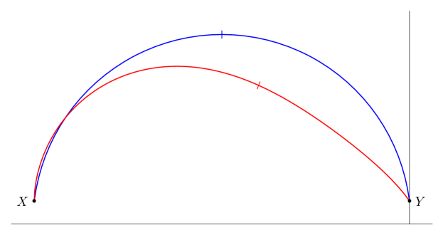
Figure 7: A Teichmüller geodesic (blue) and a stretch path (red) in the Teichmüller space $\mathcal{T}(S_{1,1})\simeq\mathbf{H}$ of the punctured torus. Both geodesic segments start at $X=-16.302+i$ and end at $Y=i$, and each has its midpoint marked.

Continuing toward the proof of Theorem 3.1, we show:

Lemma 3.11.

Suppose $\alpha$ crosses a leaf $\omega$ of $\lambda$. There exists a constant $C>0$ such that if $\ell_{\alpha}(s)\geqslant\epsilon_{0}$ and $d_{\alpha}(X_{s},\lambda)\geqslant C$, then $\ell_{\alpha}(t)\mathrel{\ooalign{\raisebox{1.4pt}{$\mkern 0.2mu\scriptstyle\ast$}\cr$\asymp$\cr}}e^{t-s}\ell_{\alpha}(s)$ for all $t\geqslant s$.

Proof.

By Lemma 3.8, if $d_{\alpha}(X_{s},\lambda)>\frac{4\epsilon_{M}}{\ell_{\alpha}(s)}+2$, then

$$v_{s}\leqslant 2e^{-\frac{\ell_{\alpha}(s)}{4}d_{\alpha}(X_{s},\lambda)}.$$

Since $\ell_{\alpha}(s)\geqslant\epsilon_{0}$ in this case, there is a universal constant $C$ so that this estimate applies when $d_{\alpha}(X_{s},\lambda)>C$. Furthermore, we can choose $C$ so that the inequality above gives

$$v_{s}\leqslant\frac{1}{3}\ell_{\alpha}(s)$$

and so $h_{s}\geqslant\frac{2}{3}\ell_{\alpha}(s)$ and $2v_{s}\leqslant h_{s}$. Incorporating Lemma 3.4, we have that for all $t>s$,

$$\ell_{\alpha}(t)\geqslant h_{t}\geqslant\frac{1}{2}e^{t-s}h_{s}\geqslant\frac{1}{3}e^{t-s}\ell_{\alpha}(s).$$

On the other hand, $\ell_{\alpha}(t)\leqslant e^{t-s}\ell_{\alpha}(s)$. This finishes the proof. ∎

Lemma 3.12.

Suppose $\alpha$ interacts with $\lambda$. If $\ell_{\alpha}(t)\geqslant\epsilon_{0}$ for all $t\in[a,b]$, then $d_{\alpha}(X_{a},X_{b})\mathrel{\ooalign{\raisebox{1.6pt}{$\mkern 0.2mu\scriptscriptstyle+$}\cr$\asymp$\cr}}0$.

Proof.

We first show that for any $s\leqslant t$, if $\ell_{\alpha}(t)\mathrel{\ooalign{\raisebox{1.4pt}{$\mkern 0.2mu\scriptstyle\ast$}\cr$\asymp$\cr}}e^{t-s}\ell_{\alpha}(s)$, then $d_{\alpha}(X_{s},X_{t})\mathrel{\ooalign{\raisebox{1.6pt}{$\mkern 0.2mu\scriptscriptstyle+$}\cr$\asymp$\cr}}0$. Let $\beta$ be the shortest curve at $X_{s}$ that intersects $\alpha$. At time $t$, the length of $\beta$ satisfies

$$\ell_{\beta}(t)\geqslant\ell_{\alpha}(t)d_{\alpha}(\beta,X_{t})-D\ell_{\alpha}(t),$$

where $D\geqslant 0$ is universal. Also, $d_{\alpha}(\beta,X_{s})$ is bounded by the choice of $\beta$. Hence we can write

$$\frac{\ell_{\beta}(t)}{\ell_{\alpha}(t)}\mathrel{\ooalign{\raisebox{1.6pt}{$\mkern 0.2mu\scriptscriptstyle+$}\cr$\succ$\cr}}d_{\alpha}(X_{s},X_{t}).$$

Therefore, since $\ell_{\beta}(t)\leqslant e^{t-s}\ell_{\beta}(s)$ and $\ell_{\alpha}(t)\mathrel{\ooalign{\raisebox{1.4pt}{$\mkern 0.2mu\scriptstyle\ast$}\cr$\asymp$\cr}}e^{t-s}\ell_{\alpha}(s)$, we have

$$d_{\alpha}(X_{s},X_{t})\mathrel{\ooalign{\raisebox{1.6pt}{$\mkern 0.2mu\scriptscriptstyle+$}\cr$\prec$\cr}}\frac{\ell_{\beta}(s)}{\ell_{\alpha}(s)}.$$

Let $\epsilon_{B}$ be the Bers constant. If $\ell_{\alpha}(s)\geqslant\epsilon_{B}$, then $\ell_{\beta}(t)\leqslant\epsilon_{B}$ and so $\frac{\ell_{\beta}(s)}{\ell_{\alpha}(s)}<1$. If $\ell_{\alpha}(s)\leqslant\epsilon_{B}$, then $\ell_{\beta}(s)$ is up to a bounded multiplicative error the width of the collar about $\alpha$, So in this case, since $\ell_{\alpha}(s)\geqslant\epsilon_{0}$, we have

$$\frac{\ell_{\beta}(s)}{\ell_{\alpha}(s)}\mathrel{\ooalign{\raisebox{1.4pt}{$\mkern 0.2mu\scriptstyle\ast$}\cr$\prec$\cr}}\frac{1}{\epsilon_{0}}\log\frac{1}{\epsilon_{0}}\mathrel{\ooalign{\raisebox{1.4pt}{$\mkern 0.2mu\scriptstyle\ast$}\cr$\asymp$\cr}}1.$$

If $\alpha$ is a leaf of $\lambda$, then $\ell_{\alpha}(b)=e^{b-a}\ell_{\alpha}(a)$, so the conclusion follows from the paragraph above. Now suppose that $\alpha$ crosses a leaf of $\lambda$. Let $C$ be the constant of Lemma 3.11. If $d_{\alpha}(X_{t},\lambda)<C$ for all $t\in[a,b]$, then we are done. Otherwise, there is an earliest time $t\in[a,b]$ such that $d_{\alpha}(X_{t},\lambda)\geqslant C$. It is immediate that $d_{\alpha}(X,X_{t})\mathrel{\ooalign{\raisebox{1.6pt}{$\mkern 0.2mu\scriptscriptstyle+$}\cr$\asymp$\cr}}0$. By Lemma 3.11, $\ell_{\alpha}(b)\mathrel{\ooalign{\raisebox{1.4pt}{$\mkern 0.2mu\scriptstyle\ast$}\cr$\asymp$\cr}}e^{b-t}\ell_{\alpha}(t)$, so $d_{\alpha}(X_{t},X_{b})\mathrel{\ooalign{\raisebox{1.6pt}{$\mkern 0.2mu\scriptscriptstyle+$}\cr$\asymp$\cr}}0$ by the above paragraph. The result follows. ∎

We will now prove the theorem stated at the beginning of this section.

Proof of Theorem 3.1.

If $\ell_{\alpha}\geqslant\epsilon_{0}$, then by Lemma 3.12,

$$d_{\alpha}(X,Y)\mathrel{\ooalign{\raisebox{1.6pt}{$\mkern 0.2mu\scriptscriptstyle+$}\cr$\asymp$\cr}}0\mathrel{\ooalign{\raisebox{1.6pt}{$\mkern 0.2mu\scriptscriptstyle+$}\cr$\asymp$\cr}}\frac{1}{\ell_{\alpha}}\operatorname{Log}\frac{1}{\ell_{\alpha}}.$$

Now suppose $\ell_{\alpha}<\epsilon_{0}$ and let $[a,b]$ be the active interval for $\alpha$. From Theorem 3.10, the minimal length $\ell_{\alpha}$ occurs at $t_{\alpha}\in[a,b]$ satisfying $t_{\alpha}-a\mathrel{\ooalign{\raisebox{1.6pt}{$\mkern 0.2mu\scriptscriptstyle+$}\cr$\asymp$\cr}}\operatorname{Log}(b-t_{\alpha})$, and $\ell_{\alpha}\mathrel{\ooalign{\raisebox{1.4pt}{$\mkern 0.2mu\scriptstyle\ast$}\cr$\asymp$\cr}}e^{-(b-t_{\alpha})}$. We then have

$$\begin{split}d_{\alpha}(X_{a},X_{b})\mathrel{\ooalign{\raisebox{1.4pt}{$\mkern 0.2mu\scriptstyle\ast$}\cr$\asymp$\cr}}e^{b-a}&=e^{b-t_{\alpha}}e^{t_{\alpha}-a}\\ &\mathrel{\ooalign{\raisebox{1.4pt}{$\mkern 0.2mu\scriptstyle\ast$}\cr$\asymp$\cr}}e^{b-t_{\alpha}}e^{\operatorname{Log}(b-t_{\alpha})}\end{split}$$

If $(b-a)$ is large enough so that Theorem 3.10 gives $\operatorname{Log}(b-t_{\alpha})=\log(b-t_{\alpha})$, then this shows $d_{\alpha}(X_{a},X_{b})\mathrel{\ooalign{\raisebox{1.4pt}{$\mkern 0.2mu\scriptstyle\ast$}\cr$\asymp$\cr}}e^{b-t_{\alpha}}(b-t_{\alpha})\mathrel{\ooalign{\raisebox{1.4pt}{$\mkern 0.2mu\scriptstyle\ast$}\cr$\asymp$\cr}}\frac{1}{\ell_{\alpha}}\log(\frac{1}{\ell_{\alpha}})$, and since $\ell_{\alpha}\leqslant\epsilon_{0}$, we have $\frac{1}{\ell_{\alpha}}\log\frac{1}{\ell_{\alpha}}\mathrel{\ooalign{\raisebox{1.6pt}{$\mkern 0.2mu\scriptscriptstyle+$}\cr$\asymp$\cr}}\frac{1}{\ell_{\alpha}}\operatorname{Log}\frac{1}{\ell_{\alpha}}$ with equality for $\ell_{\alpha}$ small enough. By Lemma 3.12, $d_{\alpha}(X,X_{a})$ and $d_{\alpha}(X_{b},Y)$ are both uniformly bounded. Thus $d_{\alpha}(X,Y)\mathrel{\ooalign{\raisebox{1.6pt}{$\mkern 0.2mu\scriptscriptstyle+$}\cr$\asymp$\cr}}d_{\alpha}(X_{a},X_{b})$ and the estimate on $d_{\alpha}(X,Y)$ from Theorem 3.10 follows in this case.

Otherwise, $(b-a)$ is bounded above by a universal constant, in which case we will show $d_{\alpha}(X,Y)\mathrel{\ooalign{\raisebox{1.6pt}{$\mkern 0.2mu\scriptscriptstyle+$}\cr$\asymp$\cr}}\frac{1}{\ell_{\alpha}}\operatorname{Log}\frac{1}{\ell_{\alpha}}$ by showing that both sides are uniformly bounded. First, the upper bound on $(b-a)$ gives a positive lower bound on $\ell_{\alpha}$ (which is already bounded above by $\epsilon_{0}$) and so $\frac{1}{\ell_{\alpha}}\operatorname{Log}\frac{1}{\ell_{\alpha}}\mathrel{\ooalign{\raisebox{1.6pt}{$\mkern 0.2mu\scriptscriptstyle+$}\cr$\asymp$\cr}}0$. On the other hand, using the bound on $(b-a)$, Theorem 3.10 gives $d_{\alpha}(X_{a},X_{b})\mathrel{\ooalign{\raisebox{1.6pt}{$\mkern 0.2mu\scriptscriptstyle+$}\cr$\asymp$\cr}}0$, and as before $d_{\alpha}(X,Y)\mathrel{\ooalign{\raisebox{1.6pt}{$\mkern 0.2mu\scriptscriptstyle+$}\cr$\asymp$\cr}}d_{\alpha}(X_{a},X_{b})$. We conclude $d_{\alpha}(X,Y)\mathrel{\ooalign{\raisebox{1.6pt}{$\mkern 0.2mu\scriptscriptstyle+$}\cr$\asymp$\cr}}0$, as required.

For the last statement of Theorem 3.1, let $C$ be the constant of Lemma 3.11. By assumption $\ell_{\alpha}(t)>\epsilon_{0}$ for all $t\leqslant a$. If there exists $t\leqslant a$ such that $d_{\alpha}(X_{t},\lambda)\geqslant C$, then $\ell_{\alpha}(t_{\alpha})\mathrel{\ooalign{\raisebox{1.4pt}{$\mkern 0.2mu\scriptstyle\ast$}\cr$\asymp$\cr}}e^{t_{\alpha}-t}\ell_{\alpha}(t)$, where $t_{\alpha}$ is the time of the minimal length of $\ell_{\alpha}$. This is impossible for all sufficiently small $\ell_{\alpha}$. Finally, since $d_{\alpha}(X_{a},X_{b})\mathrel{\ooalign{\raisebox{1.4pt}{$\mkern 0.2mu\scriptstyle\ast$}\cr$\asymp$\cr}}\frac{1}{\ell_{\alpha}}\operatorname{Log}\frac{1}{\ell_{\alpha}}$, for all sufficiently small $\ell_{\alpha}$, we can guarantee that $d_{\alpha}(X_{b},\lambda)\geqslant C$. The final conclusion follows by Lemma 3.11. ∎

Recall that two curves that intersect cannot both have lengths less than $\epsilon_{M}$ at the same time. Therefore, if $\alpha$ and $\beta$ intersect and $\ell_{\alpha}<\epsilon_{0}$ and $\ell_{\beta}<\epsilon_{0}$, then their active intervals must be disjoint. This defines an ordering of $\alpha$ and $\beta$ along $\mathcal{G}$. In the next section, we will focus on the torus $S_{1,1}$ and show that the order of $\alpha$ and $\beta$ along $\mathcal{G}$ will always agree with their order in the projection of $\mathcal{G}(t)$ to the Farey graph.

4 Coarse description of geodesics in $\mathcal{T}(S_{1,1})$

4.1 Farey graph

See [Min99] for background on the Farey graph.

Let $S_{1,1}$ be the once-punctured torus and represent its universal cover by the hyperbolic plane $\mathbf{H}$. Identify the ideal boundary $\partial\mathbf{H}$ with $\mathbf{R}\cup\left\{{\infty}\right\}$. The point $\infty$ is considered an extended rational number with reduced form $1/0$. As in Section 2.2, fix a positive ordered basis for $H_{1}(S_{1,1})$ and use this to associate a slope $p/q\in\mathbf{QP}^{1}=\mathbf{Q}\cup\left\{{\infty}\right\}$ to every simple curve. In this section we pass freely between a rational number and the associated simple curve.

Given two curves $\alpha=p/q$ and $\beta=r/s$ in reduced fractions, their geometric intersection number is $|ps-rq|$. Form a graph with vertex set $\mathbf{QP}^{1}$ as follows: Connect $p/q$ and $r/s$ by an edge if $|ps-rq|=1$. The resulting graph $\mathcal{F}$ is called the Farey graph, which is also the curve graph of $S_{1,1}$. This graph embeds naturally in $\mathbf{H}\cup\partial\mathbf{H}$, with its edges realized as hyperbolic geodesics (see Figure 8). These geodesics cut $\mathbf{H}$ into ideal triangles; this is the Farey tesselation. In this tesselation, each edge bounds exactly two ideal triangles with zero relative shearing. Thus each edge of $\mathcal{F}$ is equipped with a well-defined midpoint.

Figure 8: The Farey graph.

Let $\alpha$ denote the curve with slope $1/0$. The action of $D_{\alpha}$ on curves distinct from $\alpha$ corresponds to the mapping of slopes $m\mapsto m+1$. Let $\beta_{0}\in\mathcal{F}$ be any curve with $\operatorname{i}(\alpha,\beta_{0})=1$. The associated Dehn twist family about $\alpha$ is $\beta_{n}=D_{\alpha}^{n}(\beta_{0})$. Then $\{\beta_{n}\}_{n\in\mathbf{Z}}$ is exactly the set of vertices of $\mathcal{F}$ that are connected to $\alpha$ by an edge, or equivalently, the set of curves with slope in $\mathbf{Z}$.

4.2 Markings and pivots

A marking on $S_{1,1}$ is an unordered pair of curves $\left\{{\alpha,\beta}\right\}$ such that $\operatorname{i}(\alpha,\beta)=1$. Given a marking $\left\{{\alpha,\beta}\right\}$, there are four markings that are obtained from $\mu$ by an elementary move, namely:

$$\left\{{\alpha,D_{\alpha}(\beta)}\right\},\quad\left\{{\alpha,D_{\alpha}^{-1}(\beta)}\right\},\quad\left\{{\beta,D_{\beta}(\alpha)}\right\},\quad\left\{{\beta,D_{\beta}^{-1}(\alpha)}\right\}.$$

Note that the set of markings on $S_{1,1}$ can be identified with the set of edges of $\mathcal{F}$, and two edges differ by an elementary move if and only if they bound a common triangle in the Farey tesselation of $\mathbf{H}$. Denote by $\mathcal{MG}$ the graph with markings as vertices and an edge connecting two markings that differ by an elementary move. Then $\mathcal{MG}$ has the following property.

Lemma 4.1.

For any $\mu,\mu^{\prime}\in\mathcal{MG}$, there exists a unique geodesic connecting them.

Proof.

Each edge of $\mathcal{F}$ separates $\mathbf{H}$ into two disjoint half-spaces. Let $E(\mu,\mu^{\prime})$ be the set of edges in $\mathcal{F}$ that separate the interior of $\mu$ from the interior of $\mu^{\prime}$. Set ${\overline{E}}(\mu,\mu^{\prime})=E(\mu,\mu^{\prime})\cup\left\{{\mu,\mu^{\prime}}\right\}$. Every $\nu\in E(\mu,\mu^{\prime})$ disconnects $\mu$ from $\mu^{\prime}$, and thus must appear in every geodesic from $\mu$ and $\mu^{\prime}$. Conversely, any $\nu\in\mathcal{MG}$ lying on a geodesic from $\mu$ to $\mu^{\prime}$ must lie in ${\overline{E}}(\mu,\mu^{\prime})$. For each $\nu\in{\overline{E}}(\mu,\mu^{\prime})$, let $H_{\nu}$ be the half-space in $\mathbf{H}$ containing the interior of $\mu^{\prime}$. There is a linear order on ${\overline{E}}(\mu,\mu^{\prime})=\left\{{\mu_{1}<\mu_{2}<\cdots<\mu_{n}}\right\}$ induced by the relation $\mu_{i}<\mu_{i+1}$ if and only if $H_{\mu_{i}}\supset H_{\mu_{i+1}}$. The sequence $\mu=\mu_{1},\mu_{2},\ldots,\mu_{n}=\mu^{\prime}$ is the unique geodesic path in $\mathcal{MG}$ from $\mu$ to $\mu^{\prime}$. ∎

Given two markings $\mu$ and $\mu^{\prime}$ and a curve $\alpha$, let $n_{\alpha}$ be the number of edges in ${\overline{E}}(\mu,\mu^{\prime})$ containing $\alpha$. We say $\alpha$ is a pivot for $\mu$ and $\mu^{\prime}$ if $n_{\alpha}\geqslant 2$, and $n_{\alpha}$ is the coefficient of the pivot. Let $\operatorname{Pivot}(\mu,\mu^{\prime})$ be the set of pivots for $\mu$ and $\mu^{\prime}$. This set is naturally linearly ordered as follows. Given $\alpha\in\operatorname{Pivot}(\mu,\mu^{\prime})$, let $e_{\alpha}$ be the last edge in ${\overline{E}}(\mu,\mu^{\prime})$ containing $\alpha$. Then for $\alpha,\beta\in\operatorname{Pivot}(\mu,\mu^{\prime})$, we set $\alpha<\beta$ if $e_{\alpha}$ appears before $e_{\beta}$ in $g$.

Recall that in Section 2.8 we defined the unsigned twisting (along $\alpha$) for a pair of curves $\beta,\beta^{\prime}$; this is denoted $d_{\alpha}(\beta,\beta^{\prime})$. Generalizing this, we define unsigned twisting for the pair of markings $\mu,\mu^{\prime}$ by

$$d_{\alpha}(\mu,\mu^{\prime})=\min_{\beta\subset\mu,\>\beta^{\prime}\subset\mu^{\prime}}d_{\alpha}(\beta,\beta^{\prime}),$$

where $\beta$ is a curve in $\mu$ and $\beta^{\prime}$ is a curve in $\mu^{\prime}$. Similarly we define $d_{\alpha}(\beta,\mu^{\prime})=\min_{\beta^{\prime}\subset\mu^{\prime}}d_{\alpha}(\beta,\beta^{\prime})$. In terms of these definitions, we have:

Lemma 4.2 ([Min99]).

For any $\mu,\mu^{\prime}\in\mathcal{MG}$ and curve $\alpha$, we have $n_{\alpha}\mathrel{\ooalign{\raisebox{1.6pt}{$\mkern 0.2mu\scriptscriptstyle+$}\cr$\asymp$\cr}}d_{\alpha}(\mu,\mu^{\prime})$. For $\alpha,\beta\in\operatorname{Pivot}(\mu,\mu^{\prime})$, if $\alpha<\beta$, then $d_{\alpha}(\beta,\mu^{\prime})\mathrel{\ooalign{\raisebox{1.6pt}{$\mkern 0.2mu\scriptscriptstyle+$}\cr$\asymp$\cr}}1$ and $d_{\beta}(\mu,\alpha)\mathrel{\ooalign{\raisebox{1.6pt}{$\mkern 0.2mu\scriptscriptstyle+$}\cr$\asymp$\cr}}1$. Conversely, if $n_{\alpha}$ is sufficiently large and $d_{\alpha}(\beta,\mu^{\prime})\mathrel{\ooalign{\raisebox{1.6pt}{$\mkern 0.2mu\scriptscriptstyle+$}\cr$\asymp$\cr}}1$, then $\alpha<\beta$.

Identify $\mathcal{T}(S_{1,1})$ with $\mathbf{H}$ in the usual way. Under this identification, if $e$ is an edge of $\mathcal{F}$ with endpoints $\alpha$ and $\beta$, then the set points along $e$ correspond to the set of surfaces on which $\alpha$ and $\beta$ are the shortest curves and they intersect perpendicularly. The midpoint of $e$ correspond to when the two curves have the same length. This length is a uniform constant independent of the edge $e$.

For any $X\in\mathcal{T}(S_{1,1})$, there exists an ideal triangle $\triangle$ in the Farey tessellation of $\mathbf{H}$ containing $X$. The three vertices of $\triangle$ correspond to the three shortest curves on $X$. We will define a short marking on $X$ as follows. If $X$ has at least $2$ systoles, then let $A$ be the set of systoles on $X$. If $X$ has a unique systole, then let $A$ be set consisting of the systole plus the second shortest curves on $X$. In either case, $A$ is a subset of the vertices of $\triangle$, so $A$ has cardinality at most $3$ and every pair of curves in $A$ correspond to an edge in $\triangle$. A short marking on $X$ is any pair of curves in $A$. Note that in our definition, there is either a unique marking or three short markings on $X$. This implies that, given $X,Y\in\mathcal{T}(S_{1,1})$, there are well-defined short markings $\mu_{X}$ and $\mu_{Y}$ on $X$ and $Y$ such that $d_{\mathcal{MG}}(\mu_{X},\mu_{Y})$ is minimal among all short markings on $X$ and $Y$. By Lemma 4.1, the geodesic from $\mu_{X}$ to $\mu_{Y}$ is unique. Note that any edge of $E(\mu_{X},\mu_{Y})$ separates $\mu_{X}$ from $\mu_{Y}$, and hence it separates $X$ from $Y$. We will denote by $\operatorname{Pivot}(X,Y)=\operatorname{Pivot}(\mu_{X},\mu_{Y})$ and refer to $\operatorname{Pivot}(X,Y)$ as the set of pivots for $X$ and $Y$.

Given $X,Y\in\mathcal{T}(S_{1,1})$, we have that $d_{\alpha}(X,Y)\mathrel{\ooalign{\raisebox{1.6pt}{$\mkern 0.2mu\scriptscriptstyle+$}\cr$\asymp$\cr}}d_{\alpha}(\mu_{X},\mu_{Y})$.

Let $\epsilon_{0}$ be the constant of the previous section. The following statements establish Theorem 1.3 of the introduction.

Theorem 4.3.

Suppose $X,Y\in\mathcal{T}_{\epsilon_{0}}(S_{1,1})$ and let $\mathcal{G}(t)$ be any geodesic from $X$ to $Y$, parameterized by an interval $I\subset\mathbf{R}$. Let $\ell_{\alpha}=\inf_{t}\ell_{\alpha}(t)$. There are positive constants $\epsilon_{1}$, $C_{1}$, and $C_{2}$ such that

1. If $\ell_{\alpha}\leqslant\epsilon_{1}$, then $\alpha\in\operatorname{Pivot}(X,Y)$ and $d_{\alpha}(X,Y)\geqslant C_{1}$.

2. If $d_{\alpha}(X,Y)\geqslant C_{2}$, then $\ell_{\alpha}\leqslant\epsilon_{1}$ and $\alpha\in\operatorname{Pivot}(X,Y)$.

3. Suppose $\alpha$ and $\beta$ are distinct curves such that there exist $s,t\in I$ with $\ell_{\alpha}(s)\leqslant\epsilon_{1}$ and $\ell_{\beta}(t)\leqslant\epsilon_{1}$. Then $\alpha<\beta$ in $\operatorname{Pivot}(X,Y)$ if and only if $s<t$.

4. For any $\alpha\in\operatorname{Pivot}(X,Y)$, $\ell_{\alpha}\mathrel{\ooalign{\raisebox{1.4pt}{$\mkern 0.2mu\scriptstyle\ast$}\cr$\prec$\cr}}1$.

Proof.

The proof will show that any sufficiently small $\epsilon_{1}$ works. We first require $\epsilon_{1}<\epsilon_{0}$ where $\epsilon_{0}$ is the constant selected in the previous section.

Let $\lambda=\Lambda(X,Y)$. On the torus, every curve $\alpha$ interacts with $\lambda$. If $\lambda$ contains $\alpha$, then $\ell_{\alpha}(t)=e^{t}\ell_{\alpha}(X)$. But this implies $\ell_{\alpha}=\ell_{X}(\alpha)\geqslant\epsilon_{0}$ and $d_{\alpha}(X,Y)\mathrel{\ooalign{\raisebox{1.6pt}{$\mkern 0.2mu\scriptscriptstyle+$}\cr$\asymp$\cr}}0$ by Lemma 3.12. Thus, we may assume that $\alpha$ crosses a leaf of $\lambda$. By Theorem 3.1, $d_{\alpha}(X,Y)\mathrel{\ooalign{\raisebox{1.4pt}{$\mkern 0.2mu\scriptstyle\ast$}\cr$\asymp$\cr}}\frac{1}{\ell_{\alpha}}\log\frac{1}{\ell_{\alpha}}$. Since $d_{\alpha}(X,Y)\mathrel{\ooalign{\raisebox{1.6pt}{$\mkern 0.2mu\scriptscriptstyle+$}\cr$\asymp$\cr}}d_{\alpha}(\mu_{X},\mu_{Y})\mathrel{\ooalign{\raisebox{1.6pt}{$\mkern 0.2mu\scriptscriptstyle+$}\cr$\asymp$\cr}}n_{\alpha}$ (the latter by Lemma 4.2), we can select $\epsilon_{1}$ small enough and $C_{1}>0$ so that $\ell_{\alpha}\leqslant\epsilon_{1}$ implies that $d_{\alpha}(X,Y)\geqslant C_{1}$ and that $n_{\alpha}\geqslant 2$, i.e. $\alpha$ is a pivot. This gives (i). Using the same approximate equalities, if $d_{\alpha}(X,Y)$ is large we find that $\ell_{\alpha}$ is small, and we can select $C_{2}$ satisfying (ii).

We now fix our constants $\epsilon_{1}$, $C_{1}$ and $C_{2}$ so (i) and (ii) are satisfied. By fixing these constants, we can now ignore the dependence of any additive or multiplicative errors on them.

For (iii), suppose $\ell_{\alpha}\leqslant\epsilon_{1}$ and $\ell_{\beta}\leqslant\epsilon_{1}$. By (i), they are both pivots. Let $[a,b]$ be the active interval for $\alpha$. Recall that that this is the longest interval such that $\ell_{\alpha}(a)=\ell_{\beta}(b)=\epsilon_{0}$. Recall that by Corollary 3.7 we have $\ell_{\alpha}(t)<\epsilon_{M}$ for all $t\in[a,b]$. Similarly, let $[c,d]$ be the active interval for $\beta$. On the torus, two curves always intersect, so $\alpha$ and $\beta$ cannot be simultaneously shorter than $\epsilon_{M}$, so $[a,b]$ and $[c,d]$ must be disjoint. By Lemma 4.2, $\alpha<\beta$ if and only if $d_{\alpha}(\beta,\mu_{Y})\mathrel{\ooalign{\raisebox{1.6pt}{$\mkern 0.2mu\scriptscriptstyle+$}\cr$\asymp$\cr}}1$. By Theorem 3.1 and Lemma 3.12, $b<c$ if and only if $d_{\alpha}(X_{c},Y)\mathrel{\ooalign{\raisebox{1.6pt}{$\mkern 0.2mu\scriptscriptstyle+$}\cr$\asymp$\cr}}1$. Since $\beta$ is $\epsilon_{0}$–short on $X_{c}$, we have $d_{\alpha}(\beta,\mu_{Y})\mathrel{\ooalign{\raisebox{1.6pt}{$\mkern 0.2mu\scriptscriptstyle+$}\cr$\asymp$\cr}}d_{\alpha}(X_{c},Y)$. This finishes (iii).

Before we prove (iv), we introduce some notation. For each curve $\alpha$, let $H_{\alpha}\subset\mathcal{T}(S_{1,1})$ be the set of hyperbolic structures where $\ell_{\alpha}(X)\leqslant\epsilon_{1}$. Since $\epsilon_{1}<\epsilon_{M}$, the sets $H_{\alpha}$ and $H_{\beta}$ are disjoint if $\alpha\neq\beta$. Let $e$ be an edge of $\mathcal{F}$ and denote its endpoints by $\alpha$ and $\beta$. The segment of $e$ outside of $H_{\alpha}$ and $H_{\beta}$ is a closed interval containing the midpoint of $e$. Along this interval, the length of $\alpha$ and $\beta$ is uniformly bounded (by a constant that depends only on $\epsilon_{1}$).

To prove (iv), let $\alpha\in\operatorname{Pivot}(X,Y)$ and assume $\ell_{\alpha}>\epsilon_{1}$. Let $e\in E(\mu_{X},\mu_{Y})$ be an edge containing $\alpha$. Let $\beta$ be the other curve of $e$. The edge $e$ separates $X$ and $Y$, so any geodesic $\mathcal{G}(t)$ from $X$ to $Y$ must cross $e$ at some point $X_{t}$. If $\ell_{\beta}(t)>\epsilon_{1}$, then neither $\alpha$ or $\beta$ is $\epsilon_{1}$–short on $X_{t}$, so $X_{t}$ lies in the segment of $e$ outside of $H_{\alpha}$ and $H_{\beta}$. Hence $\ell_{\alpha}(t)\mathrel{\ooalign{\raisebox{1.4pt}{$\mkern 0.2mu\scriptstyle\ast$}\cr$\prec$\cr}}1$ by the discussion in the previous paragraph. On the other hand, if $\ell_{\beta}(t)\leqslant\epsilon_{1}$, then $\beta$ is a pivot by (i). Either $\alpha<\beta$ or $\beta<\alpha$ in $\operatorname{Pivot}(X,Y)$. If $\alpha<\beta$, then $d_{\beta}(X,\alpha)\mathrel{\ooalign{\raisebox{1.6pt}{$\mkern 0.2mu\scriptscriptstyle+$}\cr$\asymp$\cr}}1$ by Lemma 4.2. Let $[a,b]$ be the active interval for $\beta$. By Theorem 3.1 we have $d_{\beta}(X,X_{a})\mathrel{\ooalign{\raisebox{1.6pt}{$\mkern 0.2mu\scriptscriptstyle+$}\cr$\asymp$\cr}}1$, and $d_{\beta}$ satisfies the triangle inequality up to additive error (by [MM00, Equation 2.5]), so we conclude $d_{\beta}(\alpha,X_{a})\mathrel{\ooalign{\raisebox{1.6pt}{$\mkern 0.2mu\scriptscriptstyle+$}\cr$\asymp$\cr}}1$. This, together with $\ell_{\beta}(a)=\epsilon_{0}$, yields $\ell_{\alpha}(a)\mathrel{\ooalign{\raisebox{1.4pt}{$\mkern 0.2mu\scriptstyle\ast$}\cr$\asymp$\cr}}1$. If $\beta<\alpha$, then the same argument using $X_{b}$ and $Y$ in place of $X_{a}$ and $X$ also yields $\ell_{\alpha}(b)\mathrel{\ooalign{\raisebox{1.4pt}{$\mkern 0.2mu\scriptstyle\ast$}\cr$\asymp$\cr}}1$. This concludes the proof. ∎

5 Envelopes in $\mathcal{T}(S_{1,1})$

5.1 Fenchel-Nielsen coordinates along stretch paths in $\mathcal{T}(S_{1,1})$

We now focus on the once-punctured torus $S_{1,1}$, and on the completions $\alpha^{\pm}$ of the maximal chain-recurrent laminations containing a simple closed curve $\alpha$ discussed in Section 2.2.

Consider the curve $\alpha$ as a pants decomposition of $S_{1,1}$ and define $\tau_{\alpha}(X)$ to be the Fenchel-Nielsen twist coordinate of $X$ relative to $\alpha$. Note that $\tau_{\alpha}(X)$ is well defined up to a multiple of $\ell_{\alpha}(X)$, and after making a choice at some point, $\tau_{\alpha}(X)$ is well defined. The Fenchel-Nielsen theorem states that the pair of functions $\big{(}\log\ell_{\alpha}({\mathchoice{\mkern 1.0mu\mbox{\raise 2.2pt\hbox{$\centerdot$}}\mkern 1.0mu}{\mkern 1.0mu\mbox{\raise 2.2pt\hbox{$\centerdot$}}\mkern 1.0mu}{\mkern 1.5mu\centerdot\mkern 1.5mu}{\mkern 1.5mu\centerdot\mkern 1.5mu}}),\tau_{\alpha}({\mathchoice{\mkern 1.0mu\mbox{\raise 2.2pt\hbox{$\centerdot$}}\mkern 1.0mu}{\mkern 1.0mu\mbox{\raise 2.2pt\hbox{$\centerdot$}}\mkern 1.0mu}{\mkern 1.5mu\centerdot\mkern 1.5mu}{\mkern 1.5mu\centerdot\mkern 1.5mu}})\big{)}$ define a diffeomorphism of $\mathcal{T}(S_{1,1})\to\mathbf{R}^{2}$.

Each $\alpha^{\pm}$ defines a foliation $\mathcal{F}_{\alpha}^{\pm}$ on $\mathcal{T}(S_{1,1})$ whose leaves are the $\alpha^{\pm}$-stretch paths. In the $\alpha^{\pm}$ shearing coordinate system, the image of $\mathcal{T}(S_{1,1})$ in $\mathbf{R}^{2}$ is a convex cone, and the foliation $\mathcal{F}_{\alpha}^{\pm}$ are by open rays from the origin.

In this section we denote a point on the $\alpha^{\pm}$ stretch path through $X$ by $X_{t}^{\pm}=\operatorname{stretch}(X,\alpha^{\pm},t)$. The function $\log\ell_{\alpha}(X_{t}^{\pm})=\log\ell_{\alpha}(X)+t$ is smooth in $t$. Our first goal is to establish the following theorem.

Theorem 5.1.

For any simple closed curve $\alpha$ on $S_{1,1}$ and any point $X=X_{0}\in\mathcal{T}(S_{1,1})$, the functions $\tau_{\alpha}(X_{t}^{\pm})$ are smooth in $t$. Further,

$$\tau_{\alpha}(X_{t}^{+})>\tau_{\alpha}(X_{t}^{-})\qquad\text{and}\qquad\frac{d}{dt}\tau_{\alpha}(X_{t}^{+})\big{|}_{t=0}>\frac{d}{dt}\tau_{\alpha}(X_{t}^{-})\big{|}_{t=0}.$$

That is, the pair of foliations $\mathcal{F}_{\alpha}^{+}$ and $\mathcal{F}_{\alpha}^{-}$ are smooth and transverse.

We proceed to prove smoothness of $\tau_{\alpha}(X_{t}^{+})$. Recall that the $\alpha^{+}$ shearing embedding is $s_{\alpha^{+}}(X)=(\ell_{\alpha}(X),s_{\alpha}(X))$ where $s_{\alpha}(X)$ was defined in Section 2.5, and that like $\tau_{\alpha}$, the function $s_{\alpha}$ is defined only up to a adding an integer multiple of $\ell_{\alpha}(X)$. To further lighten our notation, we will often write $\ell_{\alpha}(t)$ instead of $\ell_{\alpha}(X^{+}_{t})$, and $s_{\alpha}(t)$ for $s_{\alpha}(X^{+}_{t})$.

We also denote $\tau_{\alpha}(0)$ and $\ell_{\alpha}(0)$ by $\tau_{0}$ and $\ell_{0}$ respectively. Note that the values of $\tau_{\alpha}$ and $\ell_{\alpha}$ do not depend on the choice of $\alpha^{+}$ or $\alpha^{-}$ but the values of the shearing coordinates do.

We know, from the description of stretch paths in Section 2.7, that

$$s_{\alpha}(t)=s_{\alpha}(0)e^{t}\quad\text{and}\quad\ell_{\alpha}(t)=\ell_{0}\,e^{t}.$$

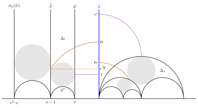
Figure 9: Computing the Fenchel-Nielsen twist along the $\alpha^{+}$ stretch path.

We can now compute $\tau_{\alpha}(X_{t}^{+})$ as follows, referring to Figure 9. Fix a lift ${\widetilde{\alpha}}$ of $\alpha$ to be the imaginary line (shown in blue in Figure 9) in the upper half-plane $\mathbf{H}$. Now develop the picture on both sides of ${\widetilde{\alpha}}$. Since we are considering $\alpha^{+}$, all the triangles on the left of ${\widetilde{\alpha}}$ are asymptotic to $\infty$ and all the triangles on the right of ${\widetilde{\alpha}}$ are asymptotic to $0$. Below we will choose some normalization, but first note that the hyperelliptic involution exchanges the two complementary triangles $T$ and $T^{\prime}$ of $\alpha^{+}$ while preserving $\alpha$ as a set. Let $\iota\colon\,\mathbf{H}\to\mathbf{H}$ be a lift of this involution chosen to preserve ${\widetilde{\alpha}}$, which therefore has the form $\iota(z)=-e^{c}/z$ for some $c=c_{t}\in\mathbf{R}$. Notice that $\iota$ exchanges the two sides of ${\widetilde{\alpha}}$ and that it fixes a unique point $ie^{c/2}$ in $\mathbf{H}$.

To fix the shearing coordinate $s_{\alpha}(t)$, we make the choice of triangles in $\mathbf{H}$ required by the construction of Section 2.4. Choose two triangles $\Delta_{l}$ and $\Delta_{r}$ in $\mathbf{H}$ separated by ${\widetilde{\alpha}}$ so that one is a lift of $T$ and the other is a lift of $T^{\prime}$ and $\iota(\Delta_{r})=\Delta_{l}$. Let ${\widetilde{w}}$ be the edge of $\Delta_{l}$ that is a lift of $w$, namely, ${\widetilde{w}}=[x,\infty]$ for some $x<0$. Let $\phi_{\alpha}(z)=e^{\ell_{\alpha}}z$ be the isometry associated to ${\widetilde{\alpha}}$ oriented toward $\infty$. The image $\phi_{\alpha}({\widetilde{w}})=[e^{\ell_{\alpha}}x,\infty]$ is another lift of $w$. Let ${\widetilde{\delta}}$ be the lift of $\delta$ that is asymptotic to ${\widetilde{w}}$ and $\phi_{\alpha}({\widetilde{w}})$. By applying a further dilation to the picture if necessary, we can assume that ${\widetilde{\delta}}=[x-1,\infty]$. Now, the geodesic ${\widetilde{w}}^{\prime}=[x,x-1]$ is a lift of $w^{\prime}$.

With our normalization, the midpoint of $[x,\infty]$ associated to $\Delta_{l}$ is the point $(x,1)$. Recall that $s_{\delta}=-\ell_{\alpha}$ in this case, which is the shearing between triangles $\Delta_{l}=[x,x-1,\infty]$ and $[x-1,e^{\ell_{\alpha}}x,\infty]$. This means that their midpoints on $\tilde{\delta}$ have $y$-coordinates with ratio $e^{\ell_{\alpha}}$, i.e.

$$\frac{|e^{\ell_{\alpha}}x-(x-1)|}{|(x-1)-x|}=e^{\ell_{\alpha}}$$

from which it follows that

$$x=-\coth(\ell_{\alpha}/2).$$

Let $h_{l}$ be the endpoint on ${\widetilde{\alpha}}$ of the horocycle based at infinity containing the midpoint of $\widetilde{w}$ considered as an edge of $\Delta_{l}$. Let $h_{r}=\iota(h_{l})$, By construction, $h_{l}=1$ and $h_{r}=e^{c}$. We can normalize so that $s_{\alpha}=c$.

To visualize the Fenchel-Nielsen twist parameter $\tau_{+}(t)$ at $X_{t}$ about $\alpha$, consider the shortest geodesic arc $\beta$ with both endpoints on $\alpha$ intersecting perpendicularly (so $\beta$ only intersects $\alpha$ twice). By symmetry, this arc intersects $\delta$ at a point $q$ that is equidistant to the midpoints of $\delta$ associated to $T$ and $T^{\prime}$. We choose a lift ${\widetilde{\beta}}$ that passes through ${\widetilde{q}}=(x-1,e^{\ell_{\alpha}/2})$. Let $p_{l}$ be the endpoint on ${\widetilde{\alpha}}$ of the lift of $\beta$ that passes through ${\widetilde{\delta}}$. Since ${\widetilde{\beta}}$ is perpendicular to ${\widetilde{\alpha}}$, we have $q$ and $p_{l}$ lie on a Euclidean circle centered at the origin. Using the Pythagorean theorem, we obtain:

$$p_{l}=\sqrt{(x-1)^{2}+\left(e^{\ell_{\alpha}/2}\right)^{2}}=e^{\ell_{\alpha}/2}\coth\frac{\ell_{\alpha}}{2}.$$

Let $ip_{r}=\iota(ip_{l})=-e^{c}/ip_{l}=ie^{c}/p_{l}$. Up to an integral multiple of $\ell_{\alpha}$, the twisting $\tau_{\alpha}(t)$ is the signed distance between $ip_{l}$ and $ip_{r}$; that is

$$\tau_{\alpha} =\log\frac{p_{r}}{p_{l}}\mod\ell_{\alpha}$$

$$=\log\frac{e^{c}}{e^{\ell_{\alpha}}\coth^{2}(\frac{\ell_{\alpha}}{2})}\mod\ell_{\alpha}$$

$$=c-2\log\coth\frac{\ell_{\alpha}}{2}\mod\ell_{\alpha}\$$

$$=s_{\alpha}-2\log\coth\frac{\ell_{\alpha}}{2}\mod\ell_{\alpha}$$

In particular, at $t=0$, we obtain

$$\tau_{0}=s_{\alpha}(0)-2\log\coth\frac{\ell_{0}}{2}\mod\ell_{0}.$$ (27)

As we mentioned previously, $s_{\alpha}(t)=s_{\alpha}(0)e^{t}$ and $\ell_{\alpha}(t)=\ell_{0}e^{t}$. Hence,

$$\tau_{\alpha}(t)=e^{t}s_{\alpha}(0)-2\log\coth\frac{e^{t}\ell_{0}}{2}\mod\ell_{\alpha}.$$

Solving for $\tau_{0}$ using (27), we obtain

$$\tau_{\alpha}\big{(}X_{t}^{+}\big{)}=e^{t}\tau_{0}+2e^{t}\log\coth\frac{\ell_{0}}{2}-2\log\coth\frac{e^{t}\,\ell_{0}}{2}\mod\ell_{\alpha}.$$ (28)

Now let $X_{t}^{-}$ be the stretch path starting from $X$ associated to $\alpha^{-}$. The computation in this case is similar; in fact $2\tau=s_{\alpha}^{+}+s_{\alpha}^{-}\mod\ell_{\alpha}$. Thus

$$\tau_{\alpha}\big{(}X_{t}^{-}\big{)}=e^{t}\tau_{0}-2e^{t}\log\coth\frac{\ell_{0}}{2}+2\log\coth\frac{e^{t}\ell_{0}}{2}\mod\ell_{\alpha}.$$ (29)

This shows that $\tau(X_{t}^{+})$ and $\tau(X_{t}^{-})$ are both smooth functions of $t$. Note that $\tau(X_{t}^{+})-\tau(X_{t}^{-})$ is well-defined. By a simple computation, we see that $\tau(X_{t}^{+})-\tau(X_{t}^{-})>0$, and

$$\frac{d}{dt}\Big{(}\tau_{\alpha}(X_{t}^{+})-\tau_{\alpha}(X_{t}^{-})\Big{)}\Big{|}_{t=0}=4\log\coth\frac{\ell_{0}}{2}+2\ell_{0}\tanh\frac{\ell_{0}}{2}\operatorname{csch}^{2}\frac{\ell_{0}}{2}>0.$$

This finishes the proof of Theorem 5.1.

5.2 Structure of envelopes in general

For any surface $S$ of finite type and a chain-recurrent lamination $\lambda$ on $S$ and $X\in\mathcal{T}(S)$, define

$$\operatorname{Out}(X,\lambda)=\left\{{Z\in\mathcal{T}(S)\>\colon\>\lambda=\Lambda(X,Z)}\right\}\quad\text{and}\quad\operatorname{In}(X,\lambda)=\left\{{Z\in\mathcal{T}(S)\>\colon\>\lambda=\Lambda(Z,X)}\right\}.$$

We call these the out-envelope and in-envelope of $X$ (respectively) in the direction $\lambda$.

Proposition 5.2.

The out-envelopes and in-envelopes have the following properties.

1. If $\lambda$ is maximal chain-recurrent, then for any completion $\widehat{\lambda}$ of $\lambda$, the set $\operatorname{Out}(X,\lambda)$ is the stretch ray starting at $X$ associated to $\widehat{\lambda}$, and the set $\operatorname{In}(X,\lambda)$ is the stretch ray associated to $\widehat{\lambda}$ ending at $X$.

2. The closure of $\operatorname{Out}(X,\lambda)$ consists of points $Y$ with $\lambda\subset\Lambda(X,Y)$. Similarly, the closure of $\operatorname{In}(X,\lambda)$ is the set of points $Y$ with $\lambda\subset\Lambda(X,Y)$.

3. If $\lambda$ is a simple closed curve, then $\operatorname{Out}(X,\lambda)$ and $\operatorname{In}(X,\lambda)$ are open sets.

Proof.

First assume $\lambda$ is maximal chain-recurrent and let $\widehat{\lambda}$ be a completion of it. By Corollary 2.3, if $\Lambda(X,Y)=\lambda$, then there exists $t>0$ such that $Y=\operatorname{stretch}(X,\widehat{\lambda},t)$ and this is the only geodesic from $X$ to $Y$. That is, any point in $\operatorname{Out}(X,\lambda)$ can be reached from $X$ by following the stretch ray along $\widehat{\lambda}$ starting at $X$. Similarly if $Y\in\operatorname{In}(X,\lambda)$, then the stretch ray along $\widehat{\lambda}$ starting at $Y$ contains $X$, or equivalently, the stretch ray along $\widehat{\lambda}$ ending at $X$ contains $Y$. This is (i).

For the other statements, we use [Thu86c, Theorem 8.4], which shows that if $Y_{i}$ converges $Y$, then any limit point of $\Lambda(X,Y_{i})$ in the Hausdorff topology is contained in $\Lambda(X,Y)$. Applying this to a point $Y$ in the closure of $\operatorname{Out}(X,\lambda)$, and a sequence $Y_{i}\in\operatorname{Out}(X,\lambda)$ converging to $Y$, we obtain $\lambda\subset\Lambda(X,Y)$. For the other direction of (ii), let $Y$ be any point such that $\lambda\subset\Lambda(X,Y)$. To show $Y$ is in the closure of $\operatorname{Out}(X,\lambda)$, we find a point $Z\in\operatorname{Out}(X,\lambda)$ such that $d_{\text{Th}}(Y,Z)=\epsilon$, for any $\epsilon$. Let $\lambda^{\prime}$ be any maximal chain-recurrent lamination such that $\lambda=\lambda^{\prime}\cap\Lambda(X,Y)$, and let $Z=\operatorname{stretch}(Y,\lambda^{\prime},\epsilon)$. We have $d_{\text{Th}}(Y,Z)=\epsilon$. Since $\lambda=\lambda^{\prime}\cap\Lambda(X,Y)$, we must have $\Lambda(X,Z)=\lambda$. This shows (ii) for $\operatorname{Out}(X,\lambda)$. The analogous statement for $\operatorname{In}(X,\lambda)$ is proven similarly.

To obtain (iii), let $\lambda$ be a simple closed curve, $Y\in\operatorname{Out}(X,\lambda)$, and $Y_{i}$ is any sequence converging to $Y$, then any limit point of $\Lambda(X,Y_{i})$ is contained in $\lambda$. Since $\lambda$ is a simple closed curve, $\Lambda(X,Y_{i})=\lambda$ for all sufficiently large $i$. This shows $\operatorname{Out}(X,\lambda)$ is open. The same proof also applies to $\operatorname{In}(X,\lambda)$. ∎

Let $X,Y\in\mathcal{T}(S)$, and denote $\lambda=\Lambda(X,Y)$. We define the envelope of geodesics from $X$ to $Y$ to be the set

$$\operatorname{Env}(X,Y)=\Big{\{}{Z\>\colon\>Z\in[X,Y]\text{ for some geodesic }[X,Y]}\Big{\}}.$$

Proposition 5.3.

For any $X,Y\in\mathcal{T}(S)$, $\operatorname{Env}(X,Y)=\overline{\operatorname{Out}\big{(}X,\lambda\big{)}}\cap\overline{\operatorname{In}\big{(}Y,\lambda\big{)}}$.

Proof.

For any $Z\in\operatorname{Env}(X,Y)$, since $Z$ lies on a geodesic from $X$ to $Y$, $\lambda$ must be contained in $\Lambda(X,Z)$ and in $\Lambda(Z,Y)$. This shows $\operatorname{Env}(X,Y)\subset\overline{\operatorname{Out}(X,\lambda)}\cap\overline{\operatorname{In}(Y,\lambda)}$. On the other hand, if $Z\in\overline{\operatorname{Out}(X,\lambda)}\cap\overline{\operatorname{In}(Y,\lambda)}$, then $\lambda\subset\Lambda(X,Z)$ and $\lambda\subset\Lambda(Z,Y)$. That is, if $\mu$ is the stump of $\lambda$, then $d_{\text{Th}}(X,Z)=\log\frac{\ell_{\mu}(Z)}{\ell_{\mu}(X)}$ and $d_{\text{Th}}(Z,Y)=\log\frac{\ell_{\mu}(Y)}{\ell_{\mu}(Z)}$, so $d_{\text{Th}}(X,Y)=d_{\text{Th}}(X,Z)+d_{\text{Th}}(Z,Y)$. Thus, the concatenation of any geodesic from $X$ to $Z$ and from $Z$ to $Y$ is a geodesic from $X$ to $Y$. ∎

5.3 Structure of envelopes in $\mathcal{T}(S_{1,1})$

In this section, we specialize our study of envelopes to the case of $S=S_{1,1}$, and prove Theorem 1.1 of the introduction. The proof is divided into several propositions.

Proposition 5.4.

Let $\alpha$ be a simple closed curve on $S_{1,1}$. For any $X\in\mathcal{T}(S_{1,1})$, the set $\operatorname{Out}(X,\alpha)$ is an open region bounded by the stretch rays along $\alpha^{\pm}$ starting at $X$. Similarly, $\operatorname{In}(X,\alpha)$ is an open region bounded by the stretch rays along $\alpha^{\pm}$ ending at $X$.

Proof.

Set $X_{t}^{\pm}=\operatorname{stretch}(X,\alpha^{\pm},t)$. By Theorem 2.2, for any surface $S$ and any two points $X,Y\in\mathcal{T}(S)$, Thurston constructed a geodesic from $X$ to $Y$ that is a concatenation of stretch paths, where the number of stretch paths needed in the concatenation is bounded by $2|\chi(S)|$, i.e. the number of triangles in an ideal triangulation of $S$. In our setting where $S=S_{1,1}$, for $Y\in\operatorname{Out}(X,\alpha)$, this would be either a single stretch path or a union of two stretch paths $[X,Z]$ and $[Z,Y]$ where both $\Lambda(X,Z)$ and $\Lambda(Z,Y)$ contain $\alpha$. By Corollary 2.3, each one of these is a stretch path along either $\alpha^{+}$ or $\alpha^{-}$. The initial path can be chosen to stretch along $\alpha^{+}$ or $\alpha^{-}$ arbitrarily. Assuming we first stretch along $\alpha^{-}$, then there are $t_{1}$ and $t_{2}$ such that $Z=\operatorname{stretch}(X,\alpha^{-},t_{1})$, $Y=\operatorname{stretch}(Z,\alpha^{+},t_{2})$, and $d_{\text{Th}}(X,Y)=t_{1}+t_{2}$. Set $Z_{t}^{-}=\operatorname{stretch}(Z,\alpha^{-},t)$ and $Z_{t}^{+}=\operatorname{stretch}(Z,\alpha^{+},t)$. By the calculations of the previous section, $\tau_{\alpha}\left(Z^{-}_{t}\right)<\tau_{\alpha}(Z^{+}_{t})$. Since $Z^{-}_{t}=X^{-}_{t+t_{1}}$ and $Z^{+}_{t_{2}}=Y$, we have

$$\ell_{\alpha}\left(X^{-}_{t_{1}+t_{2}}\right)=\ell_{\alpha}(Y)\qquad\text{and}\qquad\tau_{\alpha}\left(X^{-}_{t_{1}+t_{2}}\right)<\tau_{\alpha}(Y)$$

Similarly, if we stretch along $\alpha^{+}$ first, then there are $s_{1}$ and $s_{2}$ such that $W=\operatorname{stretch}(X,\alpha^{+},s_{1})$, $Y=\operatorname{stretch}(W,\alpha^{-},s_{2})$, and $s_{1}+s_{2}=t_{1}+t_{2}$. Then $X^{+}_{t_{1}+t_{2}}=X^{+}_{s_{1}+s_{2}}$ and by the same argument as above

$$\ell_{\alpha}\left(X^{+}_{t_{1}+t_{2}}\right)=\ell_{\alpha}(Y)\qquad\text{and}\qquad\tau_{\alpha}(Y)<\tau_{\alpha}\left(X^{+}_{t_{1}+t_{2}}\right)$$

That is, $Y$ is inside of the sector bounded by the stretch rays $X_{t}^{+}$ and $X_{t}^{-}$ for $t>0$. By replacing geodesics from $X$ to $Y$ by by geodesics from $Y$ to $X$, we obtain the statement for $\operatorname{In}(X,\alpha)$. ∎

Remark 5.5 (Visualization of envelopes).

Figure 0page.1 (on the title page) illustrates Proposition 5.4 by showing the sets $\operatorname{In}(X,\alpha)$ in the Poincaré disk model of $\mathcal{T}(S_{1,1})$ for $X$ the hexagonal punctured torus and for several simple curves $\alpha$, including the three systoles. In the figure, the disk model is normalized so that the origin corresponds to the hexagonal punctured torus. This figure was produced as follows: The Fenchel-Nielsen coordinate computations of (28)–(29) make it straightforward to compute stretch paths passing through a given point in the relative $\operatorname{SL}(2,\mathbf{R})$ character variety of $\pi_{1}(S_{1,1})$. The software package CP1 [Dum13] allows the computation of the uniformization map from the disk to the relative character variety; this map was numerically inverted using Newton’s method to transport the computed stretch paths to the disk.

By the results of [Thé07], the stretch lines appearing as boundaries of in-envelopes for $\mathcal{T}(S_{1,1})$ are exactly those which limit on rational points on the circle at infinity as $t\to-\infty$. Thus Figure 0page.1 can be alternatively described as showing regions bounded by the pairs of stretch rays joining several rational points at infinity to the hexagonal punctured torus.

Corollary 5.6.

Given $X,Y\in\mathcal{T}(S_{1,1})$, if $\Lambda(X,Y)$ is a simple closed curve, then $\operatorname{Env}(X,Y)$ is a compact quadrilateral.

Proof.

The statement follows from Proposition 5.4 and the fact that $\operatorname{Env}(X,Y)=\overline{\operatorname{Out}(X,\alpha)}\cap\overline{\operatorname{In}(Y,\alpha)}$. ∎

Proposition 5.7.

In $\mathcal{T}(S_{1,1})$, the set $\,\operatorname{Env}(X,Y)$ varies continuously as a function of $X$ and $Y$ with respect to the topology induced by the Hausdorff distance on closed sets.

Proof.

First suppose $\Lambda(X,Y)$ is a simple closed curve $\alpha$. By [Thu86c, Theorem 8.4], if $X_{i}\to X$ and $Y_{i}\to Y$, then $\Lambda(X,Y)$ contains any limit point of $\Lambda(X_{i},Y_{i})$; thus $\Lambda(X_{i},Y_{i})=\alpha$ for all sufficiently large $i$. That is, for sufficiently large $i$, $\operatorname{Env}(X_{i},Y_{i})$ is a compact quadrilateral bounded by segments in the foliations $\mathcal{F}_{\alpha}^{\pm}$. Let $Z$ be the left corner of $\operatorname{Env}(X,Y)$, i.e. the intersection point of the leaf of $\mathcal{F}^{+}_{\alpha}$ through $X$ and the leaf of $\mathcal{F}^{-}_{\alpha}$ through $Y$. For any neighborhood $U$ of $Z$, by smoothness and transversality of $\mathcal{F}_{\alpha}^{\pm}$, there is a neighborhood $U_{X}$ of $X$ and a neighborhood $U_{Y}$ of $Y$, such that for all sufficiently large $i$, $X_{i}\in U_{X}$, $Y_{i}\in U_{Y}$, and the leaf of $\mathcal{F}^{+}_{\alpha}$ through $X_{i}$ and the leaf of $\mathcal{F}^{-}_{\alpha}$ through $Y_{i}$ will intersect in $U$. That is, for all sufficiently large $i$, the left corner of $\operatorname{Env}(X_{i},Y_{i})$ lies close to the left corner of $\operatorname{Env}(X,Y)$. A similar argument holds for the right corners. This shows $\operatorname{Env}(X_{i},Y_{i})$ converges to $\operatorname{Env}(X,Y)$.

Now suppose $\Lambda(X,Y)=\lambda$ is a maximal chain-recurrent lamination and $X_{i}\to X$ and $Y_{i}\to Y$. Let $\widehat{\lambda}$ be the canonical completion of $\lambda$, and let $\mathcal{G}$ be the stretch path along $\widehat{\lambda}$ passing through $X$ and $Y$. Also let $\mathcal{G}_{i}$ and $\mathcal{G}_{i}^{\prime}$ be the stretch paths along $\widehat{\lambda}$ through $X_{i}$ and $Y_{i}$ respectively. Since stretch paths along $\widehat{\lambda}$ foliate $\mathcal{T}(S_{1,1})$, $\mathcal{G}_{i}$ and $\mathcal{G}_{i}^{\prime}$ either coincide or are disjoint. In the backward direction, all stretch paths along $\widehat{\lambda}$ converge to $\lambda$ (the stump of $\widehat{\lambda}$) in $\mathcal{PML}$ [Pap91]. If they coincide, then $\Lambda(X_{i},Y_{i})=\lambda$ and $\operatorname{Env}(X_{i},Y_{i})$ is a segment of $\mathcal{G}_{i}$. If they are disjoint, then they divide $\mathcal{T}(S_{1,1})$ into three disjoint regions. Let $M_{i}$ be the closure of the region bounded by $\mathcal{G}_{i}\cup\mathcal{G}_{i}^{\prime}$; see Figure 10. In the case that $\mathcal{G}_{i}=\mathcal{G}_{i}^{\prime}$, set $M_{i}=\mathcal{G}_{i}$. For any geodesic $L$ from $X_{i}$ to $Y_{i}$, since $X_{i},Y_{i}\in M_{i}$, if $L$ leaves $M_{i}$, then it must cross either $\mathcal{G}_{i}$ or $\mathcal{G}_{i}^{\prime}$ at least twice. But two points on a stretch path cannot be connected by any other geodesic in the same direction, so $L$ must be contained entirely in $M_{i}$. Therefore, $\operatorname{Env}(X_{i},Y_{i})\subset M_{i}$ (see Figure 10). Since $\mathcal{G}_{i}$ and $\mathcal{G}_{i}^{\prime}$ converge to $\mathcal{G}$, $M_{i}$ also converges to $\mathcal{G}$. Therefore $\operatorname{Env}(X_{i},Y_{i})$ converges to a subset of $\mathcal{G}$. For any $Z_{i}\in\operatorname{Env}(X_{i},Y_{i})$, $d_{\text{Th}}(X_{i},Z_{i})+d_{\text{Th}}(Z_{i},Y_{i})=d_{\text{Th}}(X_{i},Y_{i})$, so by continuity of $d_{\text{Th}}$, $Z_{i}$ must converge to a point $Z\in\mathcal{G}$ with $d_{\text{Th}}(X,Z)+d_{\text{Th}}(Z,Y)=d_{\text{Th}}(X,Y)$. In other words, $Z$ lies on the geodesic from $X$ to $Y$. This shows $\operatorname{Env}(X_{i},Y_{i})$ converges to $\operatorname{Env}(X,Y)$. ∎

Figure 10: $\operatorname{Env}(X_{i},Y_{i})$ is sandwiched between $\mathcal{G}_{i}$ and $\mathcal{G}_{i}^{\prime}$.

We can now assemble the proof of Theorem 1.1: Part (ii) is Proposition 5.7, part (iii) is Proposition 5.2(i), and part (iv) is Corollary 5.6. Part (i) is immediate by Corollary 5.6 for simple closed curves and by part (iii) for the remaining case.

6 Thurston norm and rigidity

In this section we introduce and study Thurston’s norm, which is the infinitesimal version of the metric $d_{\text{Th}}$, and prove Theorems 1.4 and 1.5.

6.1 The norm

Thurston showed in [Thu86c] that the metric $d_{\text{Th}}$ is Finsler, i.e. it is induced by a norm $\left\|{{\mathchoice{\mkern 1.0mu\mbox{\raise 2.2pt\hbox{$\centerdot$}}\mkern 1.0mu}{\mkern 1.0mu\mbox{\raise 2.2pt\hbox{$\centerdot$}}\mkern 1.0mu}{\mkern 1.5mu\centerdot\mkern 1.5mu}{\mkern 1.5mu\centerdot\mkern 1.5mu}}}\right\|_{\mathrm{Th}}$ on the tangent bundle. This norm is naturally expressed as the infinitesimal analogue of the length ratio defining $d_{\text{Th}}$:

$$\left\|{v}\right\|_{\mathrm{Th}}=\sup_{\alpha}\frac{d_{X}\ell_{\alpha}(v)}{\ell_{\alpha}(X)}=\sup_{\alpha}d_{X}(\log\ell_{\alpha})(v),\;\;v\in T_{X}\mathcal{T}(S)$$ (30)

The following regularity of the norm will be needed in our study of isometries of Thurston’s metric:

Theorem 6.1.

Let $S$ be a surface of finite hyperbolic type. Then the Thurston norm function $T\mathcal{T}(S)\to\mathbf{R}$ is locally Lipschitz.

The Thurston norm is defined as a supremum of a collection of $1$-forms; we will deduce its regularity from that of the forms. In preparation for stating a result to that effect, we must introduce some terminology.

Let $M$ be a smooth manifold, let $\pi:V\to M$ be a vector bundle over $M$, and let $\mathcal{E}$ be a collection of sections of $V$. We say that $\mathcal{E}$ is locally uniformly bounded if for each $x\in M$ there exists a neighborhood $U$ of $x$ and a compact set $K\subset V$ such that for each $y\in U$ and $e\in\mathcal{E}$ we have $e(y)\in K$. We say that $\mathcal{E}$ is locally uniformly Lipschitz if for each $x\in M$ there exists a neighborhood $U$ of $x$, a local trivialization $\varphi:\pi^{-1}(U)\xrightarrow{\sim}U\times\mathbf{R}^{n}$, and a constant $M$ so that for each $e\in\mathcal{E}$, if we use the local trivialization $\varphi$ to regard the section $e$ as a map $U_{i}\to\mathbf{R}^{n}$, then this function is $M$-Lipschitz. Here we fix any background norm on $\mathbf{R}^{n}$ in order to define Lipschitz functions to that space; because all such norms are bi-Lipschitz equivalent, the definition of locally uniformly Lipschitz does not depend on that choice.

Lemma 6.2.

Let $M$ be a smooth manifold and $\mathcal{E}$ a collection of $1$-forms on $M$. Suppose that $\mathcal{E}$, considered as a collection of sections of $T^{*}M$, is locally uniformly bounded and locally uniformly Lipschitz. Then the function $E:TM\to\mathbf{R}$ defined by

$$E(v):=\sup_{e\in\mathcal{E}}e(v)$$

is locally Lipschitz (assuming it is finite at one point).

Note that “locally Lipschitz” is a well-defined property of a function on a smooth manifold or a section of a vector bundle; it is equivalent to saying that the collection consisting of only that section (or function) is locally uniformly Lipschitz.

Proof.

Any linear function $\mathbf{R}^{n}\to\mathbf{R}$ is Lipschitz, however the Lipschitz constant is proportional to its norm as an element of $(\mathbf{R}^{n})^{*}$. Thus, for example, a family of linear functions is uniformly Lipschitz only when the corresponding subset of $(\mathbf{R}^{n})^{*}$ is bounded.

For the same reason, if we take a family of $1$-forms on $M$ (sections of $T^{*}M$) and consider them as fiberwise-linear functions $TM\to\mathbf{R}$, then in order for these functions on $TM$ to be locally uniformly Lipschitz, we must require the sections of $T^{*}M$ to be both locally uniformly Lipschitz and locally uniformly bounded. Here, the compact set $K$ in the definition of locally uniformly bounded ensures that the pointwise norms of the sections in $T^{*}M$ are bounded in a neighborhood of any point.

Thus the hypotheses on $\mathcal{E}$ are arranged exactly so that the family of functions $TM\to\mathbf{R}$ of which $E$ is the supremum is locally uniformly Lipschitz.

The supremum of a family of locally uniformly Lipschitz functions is locally Lipschitz or identically infinity. Since the function $E$ is such a supremum, we find that it is locally Lipschitz once it is finite at one point. ∎

Proof of Theorem 6.1..

By (30), the Thurston norm is a supremum of the type considered in Lemma 6.2. Therefore, it suffices to show that the set

$$d\kern-0.80002pt\log\kern-0.50003pt\mathcal{C}:=\left\{{d\kern-0.80002pt\log\ell_{\alpha}\>\colon\>\alpha\text{ a simple curve }}\right\}$$

of $1$-forms on $\mathcal{T}(S)$ is locally uniformly bounded and locally uniformly Lipschitz.

To see this, first recall that length functions extend continuously from curves to the space $\mathcal{ML}(S)$ of measured laminations (see e.g. [Thu86b], [Bon86, Prop. 4.6]), and also that they extend from real-valued functions on Teichmüller space to holomorphic functions on the complex manifold $\mathcal{QF}(S)$ of quasi-Fuchsian representations (see [Bon96, p. 292]) in which $\mathcal{T}(S)$ is a totally real submanifold. The resulting length function $\ell_{\lambda}:\mathcal{QF}(S)\to\mathbf{C}$ depends continuously on $\lambda$ in the locally uniform topology of functions on $\mathcal{QF}(S)$ [Bon98, pp. 20–21].

For holomorphic functions, locally uniform convergence implies locally uniform convergence of derivatives of any fixed order, so we find that the derivatives of $\ell_{\lambda}$ also depend continuously on $\lambda$.

Restricting to $\mathcal{T}(S)\subset\mathcal{QF}(S)$, and noting that the length of a nonzero measured lamination does not vanish on $\mathcal{T}(S)$, we see that the $1$-form $d\kern-0.80002pt\log(\ell_{\lambda})$ on $\mathcal{T}(S)$ is real-analytic, and that the map $\lambda\mapsto d\kern-0.80002pt\log(\ell_{\lambda})$ is continuous from $\mathcal{ML}(S)\setminus\{0\}$ to the $C^{1}$ topology of $1$-forms on any compact subset of $\mathcal{T}(S)$.

Since the $1$-form $d\kern-0.80002pt\log\ell_{\lambda}$ is invariant under scaling $\lambda$, it is naturally a function (still $C^{1}$ continuous) of $[\lambda]\in\mathcal{PML}(S)=(\mathcal{ML}(S)\setminus\left\{{0}\right\})/\mathbf{R}^{+}$. Because $\mathcal{PML}(S)$ is compact, this implies that the collection of $1$-forms

$$d\kern-0.80002pt\log\kern-0.50003pt\mathcal{PML}:=\left\{{d\kern-0.80002pt\log\ell_{\lambda}\>\colon\>[\lambda]\in\mathcal{PML}(S)}\right\}$$

is locally uniformly bounded in $C^{1}$. In particular it is locally uniformly Lipschitz, and since this collection contains $d\kern-0.80002pt\log\kern-0.50003pt\mathcal{C}$, we are done. ∎

6.2 Shape of the unit sphere

Fix $X\in\mathcal{T}(S)$ for the rest of this section. Let $T^{1}_{X}\mathcal{T}(S)$ denote the unit sphere of Thurston’s norm, i.e.

$$T^{1}_{X}\mathcal{T}(S)=\{v\in T_{X}\mathcal{T}(S)\>\colon\>\left\|{v}\right\|_{\mathrm{Th}}=1\}.$$

Similarly, let $T_{X}^{\leqslant 1}\mathcal{T}(S)$ denote the unit ball of Thurston’s norm.

The dual of the convex set $T_{X}^{\leqslant 1}\mathcal{T}(S)$ has a convenient description in terms of measured laminations:

Theorem 6.3 (Thurston [Thu86c]).

The map $\mathcal{PML}(S)\to T_{X}^{*}\mathcal{T}(S)$ given by $\mu\mapsto d_{X}\log\ell_{\mu}$ embeds $\mathcal{PML}(S)$ as the boundary of a convex neighborhood of the origin. This convex neighborhood is the dual convex set of $T_{X}^{\leqslant 1}\mathcal{T}(S)$.

Unlike this dual set, a typical point in the boundary of $T_{X}^{\leqslant 1}\mathcal{T}(S)$ does not have a canonical description in terms of a lamination on $S$. However, certain points in the sphere arise from stretch paths. Specifically, let $\mathcal{CL}$ denote the set of all complete geodesic laminations on $S$. We have a map

$$v_{X}\colon\,\mathcal{CL}\to T^{1}_{X}\mathcal{T}(S)$$

where $v_{X}(\lambda)$ is the tangent vector at $t=0$ to the stretch path $t\mapsto\operatorname{stretch}(X,\lambda,t)$. This map is “dual” to the map $d_{X}\log\ell_{{\mathchoice{\mkern 1.0mu\mbox{\raise 2.2pt\hbox{$\centerdot$}}\mkern 1.0mu}{\mkern 1.0mu\mbox{\raise 2.2pt\hbox{$\centerdot$}}\mkern 1.0mu}{\mkern 1.5mu\centerdot\mkern 1.5mu}{\mkern 1.5mu\centerdot\mkern 1.5mu}}}$ in the weak sense that $d_{X}\log\ell_{\mu}(v_{X}(\lambda))=1$ if $\mu$ is a measured lamination whose support is contained in $\lambda$.

For later use, it will be important to note the continuity of the map $v_{X}$, which follows easily from the results of [Bon98]:

Lemma 6.4.

The map $v_{X}$ is continuous with respect to the Hausdorff topology on $\mathcal{CL}$.

Proof.

Let $\lambda_{n}\in\mathcal{CL}$ be a sequence that converges in the Hausdorff topology. In [Bon98, pp.20–21], Bonahon shows that the associated shearing embeddings $s_{\lambda_{n}}:\mathcal{T}(S)\to\mathbf{R}^{N}$ converge in the $C^{k}$ topology to $s_{\lambda}$ on any compact subset of $\mathcal{T}(S)$. Since stretch paths are rays from the origin in the shearing coordinates, this shows that the tangent vectors $v_{X}(\lambda_{n})$ to such stretch paths converge to $v_{X}(\lambda)$. ∎

Now we specialize to the punctured torus case. That is, for the rest of this section we assume $S=S_{1,1}$. An example of the Thurston unit sphere (circle) and its dual are shown in Figure 11. We will show that in this case, the shape of the unit sphere determines the hyperbolic structure $X$ up to the action of the mapping class group.

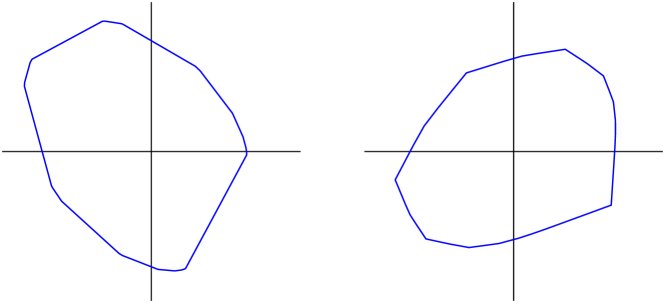
Figure 11: At left, the unit sphere $T^{1}_{X}\mathcal{T}(S_{1,1})$ of the Thurston norm on the tangent space at the point $X=0.35+1.8i$ in the upper half-plane model of $\mathcal{T}(S_{1,1})$. At right, the unit sphere of the dual norm on the cotangent space.

In [Thu86c], Thurston studies the facets of the unit ball in $T_{X}\mathcal{T}(S)$, showing in particular that they correspond to simple curves on the surface. We will require a slight extension of the result about these facets given by Thurston in Theorem 10.1 of that paper. While a corresponding result for any surface is suggested by Thurston’s work, here we will use an ad hoc argument specific to the punctured torus case.

Let $\mathcal{RL}\subset\mathcal{CL}$ be the set of canonical completions of maximal chain-recurrent geodesic laminations on $S_{1,1}$. Thus for any simple curve $\alpha$ on $S_{1,1}$ we have $\alpha^{+},\alpha^{-}\in\mathcal{RL}$, and any $\lambda\in\mathcal{RL}$ is either of this form or is a completion of a measured lamination without closed leaves.

Theorem 6.5.

Let $L$ be a support line of the unit ball of $\left\|{{\mathchoice{\mkern 1.0mu\mbox{\raise 2.2pt\hbox{$\centerdot$}}\mkern 1.0mu}{\mkern 1.0mu\mbox{\raise 2.2pt\hbox{$\centerdot$}}\mkern 1.0mu}{\mkern 1.5mu\centerdot\mkern 1.5mu}{\mkern 1.5mu\centerdot\mkern 1.5mu}}}\right\|_{\mathrm{Th}}$. Then either:

1. $L\cap T_{X}^{1}\mathcal{T}(S_{1,1})$ is a line segment with endpoints $v_{X}(\alpha^{+})$ and $v_{X}(\alpha^{-})$ for a simple curve $\alpha$, in which case $L=\{v\>\colon\>(d_{X}\log\ell_{\alpha})(v)=1\}$, or

2. $L\cap T_{X}^{1}\mathcal{T}(S_{1,1})$ is a point, and is equal to $\{v_{X}(\tilde{\lambda})\}$ for $\tilde{\lambda}$ the canonical completion of a measured lamination $\lambda$ with no closed leaves.

Proof.

First, note that Theorem 5.1 implies that $v_{X}(\alpha^{+})\neq v_{X}(\alpha^{-})$, so case (i) always yields a (nondegenerate) line segment.

By the duality between the embedding of $\mathcal{PML}(S)$ in $T_{X}^{*}\mathcal{T}(S_{1,1})$ and the norm ball $T_{X}^{\leqslant 1}\mathcal{T}(S_{1,1})$, the support lines of the latter are exactly the sets

$$L_{\mu}=\{\mu\>\colon\>(d_{X}\log\ell_{\mu})(v)=1\}$$

for nonzero $\mu\in\mathcal{ML}(S_{1,1})$. Thus it suffices to characterize the set

$$L_{\mu}^{\prime}:=L_{\mu}\cap T_{X}^{1}\mathcal{T}(S_{1,1})$$

for such $\mu$. Since $L_{\mu}$ is a support line of $T_{X}^{\leqslant 1}\mathcal{T}(S_{1,1})$, we have that $L_{\mu}^{\prime}$ is a compact convex subset of a line, i.e. either a point or a segment. If $L_{\mu}^{\prime}$ is a segment, then at any interior point $p$ of this segment the line $L_{\mu}$ is the unique support line of $T_{X}^{\leqslant 1}\mathcal{T}(S_{1,1})$ through $p$.

Suppose $\alpha$ is a simple curve. Then $v_{X}(\alpha^{\pm})\in L_{\alpha}^{\prime}$ since $\alpha\subset\alpha^{\pm}$. By convexity of $L_{\alpha}^{\prime}$, the closed segment with endpoints $v_{X}(\alpha^{\pm})$ is also a subset of $L^{\prime}$.

If $L_{\alpha}^{\prime}$ properly contained this segment, then at least one of $v_{X}(\alpha^{+})$ or $v_{X}(\alpha^{-})$ would be an interior point of $L^{\prime}$, and hence there would be a neighborhood of that point in $T_{X}^{1}\mathcal{T}(S_{1,1})$ in which $L_{\alpha}$ is the unique support line.

To see that this is not the case, choose $\lambda\in\mathcal{RL}$ that does not contain $\alpha$ (such as $\lambda=\beta^{+}$ for $\beta$ a simple curve that intersects $\alpha$). Then the sequence of Dehn twists $\lambda_{n}=D_{\alpha}^{n}(\lambda)$ converges to $\alpha^{\pm}$ in the Hausdorff topology as $n\to\pm\infty$, and the stump $\mu_{n}$ of $\lambda_{n}$ has $[\mu_{n}]\neq[\alpha]\in\mathcal{PML}(S_{1,1})$ for all $n$. By Lemma 6.4, the sequence $v_{X}(\lambda_{n})$ converges (again as $n\to\pm\infty$) to $v_{X}(\alpha^{\pm})$. Also, $v_{X}(\lambda_{n})$ lies on the support line $L_{\mu_{n}}$. Since $\mathcal{PML}(S_{1,1})$ embeds in $T_{X}^{*}\mathcal{T}(S_{1,1})$ (Theorem 6.3), the lines $L_{\mu_{n}}$ are all distinct from $L_{\alpha}$. This shows that $L_{\alpha}$ is not the unique support line in any neighborhood of $v_{X}(\alpha^{\pm})$, and that (i) holds in this case.

Now consider $L_{\mu}^{\prime}$ for $\mu$ a measured lamination with no closed leaves. Let $\tilde{\mu}\in\mathcal{RL}$ be the canonical completion of $\mu$. Then $v_{X}(\tilde{\mu})\in L_{\mu}^{\prime}$. To complete the proof we show $L_{\mu}^{\prime}=\{v_{X}(\tilde{\mu})\}$, so that these support lines give case (ii).

Suppose for contradiction that $L_{\mu}^{\prime}$ contains a nontrivial segment. Then $L_{\mu}$ is the unique support line of $T_{X}^{1}\mathcal{T}(S_{1,1})$ in the interior of that segment, which has $v_{X}(\tilde{\mu})$ in its closure.

We can approximate $\tilde{\mu}$ in the Hausdorff topology by completions $\alpha_{n}^{+}$ of simple curves $\alpha_{n}$, and can furthermore do so with $[\alpha_{n}]\in\mathcal{PML}(S)$ converging to $[\mu]\in\mathcal{PML}(S)$ from either side (recalling that $\mathcal{PML}(S)\simeq S^{1}$, so that removing $[\mu]$ separates a small neighborhood in $\mathcal{PML}(S)$ into two sides). Thus the directions of the support lines $L_{\alpha_{n}^{+}}$ can be taken to converge to that of $L_{\mu}$ from a given side. As in the previous case, Lemma 6.4 shows that $v_{X}(\alpha_{n}^{+})$ converges to $v_{X}(\tilde{\mu})$, and since $v_{X}(\alpha_{n}^{+})$ lies on $L_{\alpha_{n}}$, this convergence can be taken to be from either side of $v_{X}(\tilde{\mu})$. Since the support lines $L_{\alpha_{n}}$ are distinct from $L_{\mu}$, this shows that the support line is not unique in any interval whose closure contains $v_{X}(\tilde{\lambda})$, which is the desired contradiction. ∎

Having established that the maximal line segments in $T_{X}^{1}\mathcal{T}(S_{1,1})$ are exactly those with endpoints $v_{X}(\alpha^{\pm})$ for $\alpha$ a simple curve, we now study the geometry of these segments. From now on we refer to these simply as facets. Let $\left|{F(X,\alpha)}\right|$ denote the length of the facet corresponding to a curve $\alpha$ with respect to $\left\|{{\mathchoice{\mkern 1.0mu\mbox{\raise 2.2pt\hbox{$\centerdot$}}\mkern 1.0mu}{\mkern 1.0mu\mbox{\raise 2.2pt\hbox{$\centerdot$}}\mkern 1.0mu}{\mkern 1.5mu\centerdot\mkern 1.5mu}{\mkern 1.5mu\centerdot\mkern 1.5mu}}}\right\|_{\mathrm{Th}}$, i.e.

$$\left|{F(X,\alpha)}\right|=\left\|{v_{X}(\alpha^{+})-v_{X}(\alpha^{-})}\right\|_{\mathrm{Th}}$$

To estimate this length, we first need the following lemma.

Lemma 6.6.

Let $\operatorname{EQ}_{\alpha}(X,t)$ be the earthquake path along $\alpha$ with $\operatorname{EQ}_{\alpha}(X,0)=X$. Let $\left.\dot{\operatorname{EQ}_{\alpha}}=\frac{d\>}{dt}\operatorname{EQ}_{\alpha}(t)\right|_{t=0}$. Then we have

$$\left\|\dot{\operatorname{EQ}_{\alpha}}\right\|_{\mathrm{Th}}\mathrel{\ooalign{\raisebox{1.4pt}{$\mkern 0.2mu\scriptstyle\ast$}\cr$\asymp$\cr}}_{X}\ell_{\alpha}(X).$$

Proof.

In fact, this is true for arbitrary measured laminations, for the Teichmüller space of any surface $S$, and for any norm on $T_{X}\mathcal{T}(S)$. It is essentially just a rephrasing of [Thu86c, Theorem 5.2] and the subsequent discussion.

The map $\lambda\mapsto\dot{\operatorname{EQ}_{\lambda}}$ is a homeomorphism $\mathcal{ML}(S)\to T_{X}\mathcal{T}(S)$ (compare [Gar95, Theorem 5.1]), and in particular the tangent vector to the earthquake path of a nonzero lamination is always nonzero. The function $\lambda\mapsto\dot{\operatorname{EQ}_{\lambda}}/\ell_{\lambda}(X)$ is invariant under scaling of $\lambda$ and hence gives a well-defined continuous map $\mathcal{PML}(S)\to T_{X}\mathcal{T}\setminus\{0\}$. By compactness of $\mathcal{PML}(S)$ the function $\|\dot{\operatorname{EQ}_{\lambda}}/\ell_{\lambda}(X)\|$ is bounded above and below by positive constants, which is equivalent to the claim of the Lemma. ∎

Proposition 6.7.

For every curve $\alpha$, we have

$$\left|{F(X,\alpha)}\right|\mathrel{\ooalign{\raisebox{1.4pt}{$\mkern 0.2mu\scriptstyle\ast$}\cr$\asymp$\cr}}_{X}\ell_{\alpha}(X)^{2}\,e^{-\ell_{\alpha}(X)}.$$

Proof.

Let $X_{t}^{+}$ and $X_{t}^{-}$ be as in Section 5.1. These are paths with $X_{0}^{+}=X_{0}^{-}=X$ and with tangent vectors $v_{X}\big{(}\alpha^{+}\big{)}$ and $v_{X}\big{(}\alpha^{-}\big{)}$, respectively, at $t=0$. Note that the length of $\alpha$ is the same in $X_{t}^{+}$ and $X_{t}^{-}$, hence

$$X_{t}^{+}=\operatorname{EQ}_{\alpha}(X_{t}^{-},\Delta(t)),$$ (31)

where as before $\operatorname{EQ}_{\alpha}$ is the earthquake map along $\alpha$ and $\Delta$ is the function

$$\Delta(t)=\tau_{\alpha}(X_{t}^{+})-\tau_{\alpha}(X_{t}^{-})=4e^{t}\,\log\coth\frac{\ell_{\alpha}(X)}{2}-4\log\coth\frac{e^{t}\,\ell_{\alpha}(X)}{2}.$$

Note that $\Delta(0)=0$, and define $\dot{\Delta}=\left.\frac{d\>}{dt}{\Delta(t)}\right|_{t=0}$. Differentiating (31) at $t=0$ we find

$$\left.\frac{d\>}{dt}{X_{t}^{+}}\right|_{t=0}=(D_{1}\operatorname{EQ}_{\alpha})_{(X,0)}(\left.\frac{d\>}{dt}{X_{t}^{-}}\right|_{t=0})+(D_{2}\operatorname{EQ}_{\alpha})_{(X,0)}(\dot{\Delta})$$ (32)

Here, $D_{1}$ and $D_{2}$ denote the derivatives of $\operatorname{EQ}_{\alpha}$ with respect to its first and second arguments, respectively. Now, as observed above, the left hand side of (32) is $v_{X}\big{(}\alpha^{+}\big{)}$. Also, since $\operatorname{EQ}_{\alpha}(Y,0)=Y$ for all $Y$, we have that $(D_{1}\operatorname{EQ}_{\alpha})_{(X,0)}$ is the identity map, and the first term on the right hand side of (32) becomes $v_{X}\big{(}\alpha^{-}\big{)}$. Recalling that $\dot{\operatorname{EQ}}_{\alpha}=\left.\frac{d\>}{dt}{\operatorname{EQ}_{\alpha}(X,t)}\right|_{t=0}$, the second term on the right hand side of (32) is equal to $\dot{\Delta}\,\dot{\operatorname{EQ}}_{\alpha}$.

Thus we have

$$v_{X}\big{(}\alpha^{+}\big{)}=v_{X}\big{(}\alpha^{-}\big{)}+\dot{\Delta}\,\dot{\operatorname{EQ}}_{\alpha}$$

and hence

$$|F(X,\alpha)|=\left\|{v_{X}(\alpha^{+})-v_{X}(\alpha^{-})}\right\|_{\mathrm{Th}}=|\dot{\Delta}|\,\left\|{\dot{\operatorname{EQ}}_{\alpha}}\right\|_{\mathrm{Th}}.$$ (33)

Using the formula for $\Delta(t)$ given above we compute

$$\dot{\Delta}=4\log\coth\frac{\ell_{\alpha}(X)}{2}+4\ell_{\alpha}(X)\,\text{csch}\big{(}\ell_{\alpha}(X)\big{)}>0.$$

For large values of $x$ we have

$$\log\coth(x)\sim 2e^{-2x}\qquad\text{and}\qquad\text{csch}(x)\sim 2e^{-x}$$

Hence for large values of $\ell_{\alpha}(X)$, we have

$$|\dot{\Delta}|=\dot{\Delta}\sim 8e^{-\ell_{\alpha}(X)}+4\ell_{\alpha}(X)e^{-\ell_{\alpha}(X)}\mathrel{\ooalign{\raisebox{1.4pt}{$\mkern 0.2mu\scriptstyle\ast$}\cr$\asymp$\cr}}\ell_{\alpha}(X)e^{-\ell_{\alpha}(X)},$$

and by Lemma 6.6,

$$\left\|{\dot{\operatorname{EQ}_{\alpha}}}\right\|_{\mathrm{Th}}\mathrel{\ooalign{\raisebox{1.4pt}{$\mkern 0.2mu\scriptstyle\ast$}\cr$\asymp$\cr}}_{X}\ell_{\alpha}(X).$$

Substituting these estimates for $\dot{\Delta}$ and $\left\|{\dot{\operatorname{EQ}_{\alpha}}}\right\|_{\mathrm{Th}}$ into (33) gives the proposition. ∎

Theorem 6.8.

Let $\alpha$ and $\beta$ be curves with $\operatorname{i}(\alpha,\beta)=1$. Let $\beta_{n}=D_{\alpha}^{n}(\beta)$. Then

$$\lim_{n\to\infty}\frac{\left|{\log\left|{F(X,\beta_{n})}\right|}\right|}{n}=\ell_{\alpha}(X).$$

Proof.

For large values of $n$,

$$\ell_{\beta_{n}}(X)\mathrel{\ooalign{\raisebox{1.6pt}{$\mkern 0.2mu\scriptscriptstyle+$}\cr$\asymp$\cr}}n\ell_{\alpha}(X).$$

The theorem now follows from Proposition 6.7. ∎

Using the results above we can now show that the shape of the unit sphere in $T^{1}_{X}\mathcal{T}(S_{1,1})$ determines $X$ up to the action of the mapping class group.

Proof of Theorem 1.4.

Within the convex curve $T^{1}_{X}\mathcal{T}(S_{1,1})$ let $U_{0}$ denote an open arc disjoint from $F(X,\alpha)$ which has $v_{X}(\alpha^{+})$ as one endpoint. We use “interval notation” to refer to open arcs within $U_{0}$, where $(x,y)$ refers to the open arc in $U_{0}$ with endpoints $x,y$. Thus for example $U_{0}$ itself is $(v_{X}(\alpha^{+}),y)$ for some $y$.

Let $\mathcal{S}(U_{0})$ denote the set of curves $\gamma$ such that $F(X,\gamma)\subset U_{0}$. Thus $\mathcal{S}(U_{0})$ corresponds to the rational points of an interval in $\mathcal{PML}(S_{1,1})$ with $\alpha$ as one of its endpoints. Any sequence of simple closed geodesics in this interval converging to $\alpha$ in $\mathcal{PML}(S_{1,1})$ also converges in the Hausdorff topology, to $\alpha^{+}_{0}$.

Thus for any $\epsilon>0$, by choosing $U_{0}$ small enough we can assume that all of the curves $\gamma\in\mathcal{S}(U_{0})$ have geodesic representative in $X$ that is contained in an $\epsilon$-neighborhood of the geodesic lamination $\alpha^{+}_{0}$. This neighborhood has the structure of a thickened train track $\tau$ with three branches (as shown in Figure 12): Along $\alpha$ there is a “thick” branch and a “thin” branch, and there is a third branch $\kappa$ which connects one side of $\alpha$ to the other. Such a curve $\gamma$ is therefore determined by a pair of coprime nonnegative integers $(p,q)$, where $p$ is the weight of the thin branch along $\alpha$ and $q$ is the weight of $\kappa$. (By the switch relations, these two weights determine the weight of the thick branch to be $p+q$). We call $(p,q)$ the coordinates of $\gamma$. In terms of these coordinates, $q$ is the geometric intersection number of the curve with $\alpha$.

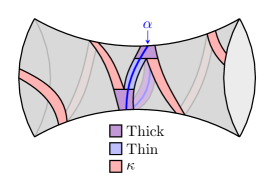
Figure 12: The train track structure of a neighborhood of $\alpha^{+}_{0}$ (shown in a collar about $\alpha$).

Let $\ell_{1}$ denote the length of the branch $\kappa$, which we define to be the minimum length of a path in the rectangle joining its short sides, and let $\ell_{\mathrm{thick}},\ell_{\mathrm{thin}}$ denote the lengths of the branches along $\alpha$. Note that $\ell_{1}$ increases without bound as $\epsilon\to 0$, so we assume from now on that $\ell_{1}$ is much larger than $\ell_{\alpha}(X)$. Also, since the union of the thick and thin branches gives a small neighborhood of $\alpha$ we have $\ell_{\mathrm{thick}}+\ell_{\mathrm{thin}}=\ell_{\alpha}(X)+O(\epsilon)$.

The point of this train track representation for curve in $\mathcal{S}(U_{0})$ is that it gives a simple estimate for hyperbolic length. Specifically, the simple curve carried by $\tau$ with coordinates $(p,q)$ breaks into $p$ arcs in $\kappa$, $q$ arcs in thin branch, and $p+q$ arcs in the thick branch. Each arc has length equal to that of its branch, up to an error proportional to $\epsilon$. Thus the overall length is

$$\begin{split}\ell(p,q)&=q\,\ell_{1}+p\,\ell_{\mathrm{thin}}+(p+q)\,\ell_{\mathrm{thick}}+O((p+q)\epsilon)\\ &=q\,(\ell_{1}+\ell_{\mathrm{thick}})+p\,(\ell_{\mathrm{thin}}+\ell_{\mathrm{thick}})+O((p+q)\epsilon)\\ &=q\,(\ell_{1}+\ell_{\mathrm{thick}})+p\,\ell_{\alpha}(X)+O((p+q)\epsilon),\end{split}$$

where the factor of $\epsilon$ accounts for the difference between the length of the branch and the length of a segment of $\gamma$ contained in the branch.

The quantity $p/q$ (the slope of the curve, for a suitable homology basis) is an affine coordinate for a neighborhood of $\alpha$ in $\mathcal{PML}(S_{1,1})\simeq\mathbf{RP}^{1}$ in which $\alpha$ corresponds to $1/0$, thus $\mathcal{S}(U_{0})$ corresponds to curves with coordinates satisfying $p/q>m$ for some constant $m\in\mathbf{R}$. By the length estimate above, after shrinking $U_{0}$ so that $\epsilon$ is much smaller than $\ell_{\alpha}(X)$ and $\ell_{1}$, we find the minimum length of a curve in $\mathcal{S}(U_{0})$ is attained for $q=1$ and the smallest integer $p$ with that $p>m$. Denote these length minimizing coordinates by $(p_{0},1)$, and the corresponding curve by $\gamma_{0}$. Note that any other curve in $\mathcal{S}(U_{0})$ has length exceeding this minimum by at least a fixed positive multiple of $\ell_{\alpha}(X)$.

By Proposition 6.7, the length of a facet corresponding to a curve whose hyperbolic length is bounded below is exponentially decreasing in length of the curve, up to a fixed multiplicative error. (Here, assuming a lower bound on the length allows us to ignore the factor $\ell_{\gamma}(X)^{2}$ in that Proposition, as it is overwhelmed by the exponential decay.) Therefore, long curves with a sufficiently large difference in hyperbolic length have associated facets whose lengths compare in the opposite way. By taking $\ell_{\alpha}(X)$ to be large enough and $U_{0}$ small enough so that all curves in $\mathcal{S}(U_{0})$ are long, the hyperbolic length gap between the minimizer $\gamma_{0}$ and any other curve in $\mathcal{S}(U_{0})$ noted above implies that $F(X,\gamma_{0})$ is the longest facet in $U_{0}$.

Now, we can shrink $U_{0}$ to exclude $F(X,\gamma_{0})$, find the new longest facet, and iterate this construction. That is, we apply the argument above to the arc $(v_{X}(\alpha^{+}),v_{X}(\gamma_{0}^{-}))$ and find hyperbolic length minimizer and facet length maximizer $\gamma_{1}$. Taking $v_{X}(\gamma_{0}^{-})$ as the endpoint means that the coordinates $(p,q)$ of curves whose facets lie in this arc now satisfy $p/q>p_{0}$, so arguing exactly as above we find that the coordinates of $\gamma_{1}$ are $(p_{0}+1,1)$. Continuing inductively we obtain a sequence $\gamma_{i}$ of curves, each corresponding to the longest facet in $(v_{X}(\alpha^{+}),v_{X}(\gamma_{i-1}^{-}))$ and having coordinates $(p_{0}+i,1)$. We call this the sequence of longest facets.

Recall that the Dehn twist about $\alpha$ acts in these coordinates by adding $1$ to the slope of the curve. Thus, in more invariant terms we have shown that the sequence of longest facets to one side of $\alpha^{+}$ corresponds to the sequence of all sufficiently large positive powers of the Dehn twist about $\alpha$ applied to a curve intersecting $\alpha$ once. This is the sort of collection considered in Theorem 6.8, which shows that the hyperbolic length of $\alpha$ is determined by the asymptotic behavior of these facet lengths.

An argument very similar to the one above shows that the sequence of longest facets in a small neighborhood of $v_{X}(\alpha^{-})$ corresponds to large negative powers of the Dehn twist about $\alpha$ applied to a curve intersecting $\alpha$ once, and that through the asymptotics of their lengths, the geometry of the norm sphere near $v_{X}(\alpha^{-})$ also determines the length of $\alpha$. As before this applies to any simple curve $\alpha$ that is sufficiently long on $X$. Collectively, we refer to the arguments above as the longest facet construction.

Now for $X,Y\in\mathcal{T}(S_{1,1})$, assume that there is a norm preserving linear map

$$L\colon\,T_{X}\mathcal{T}(S_{1,1})\to T_{Y}\mathcal{T}(S_{1,1}).$$

Since $L$ is linear, it maps the facets in $T_{X}^{1}\mathcal{T}(S_{1,1})$ bijectively to those in $T_{Y}^{1}\mathcal{T}(S_{1,1})$. By Theorem 6.5, this induces some permutation on the simple curves that label the facets: For a simple curve $\gamma$ we denote by $\gamma^{*}$ the simple curve such that $L(F(X,\gamma))=F(Y,\gamma^{*})$.

Choose a simple curve $\alpha$ so that $\ell_{X}(\alpha)$ and $\ell_{Y}(\alpha^{*})$ are large enough so that the longest facet construction applies to both of them. Then we obtain a sequence of curves $\gamma_{i}=D_{\alpha}^{i}\beta$ which satisfy $\operatorname{i}(\gamma_{i},\alpha)=1$, and whose facets $F(X,\gamma_{i})$ approach one endpoint of $F(X,\alpha)$ with each being longest in some neighborhood of that endpoint. As $L$ is an isometry, the image facets $F(X,\gamma_{i}^{*})$ approach some endpoint of $F(X,\alpha^{*})$ and are locally longest in the same sense. Thus the curves $\gamma_{i}^{*}$ are also obtained by applying powers (positive or negative) of a Dehn twist about $\alpha^{*}$ to a fixed curve and they satisfy $\operatorname{i}(\gamma_{i}^{*},\alpha^{*})=1$. Since $|F(X,\gamma_{i})|=|F(Y,\gamma_{i}^{*})|$ we conclude $\ell_{X}(\alpha)=\ell_{X}(\alpha^{*})$.

Now choose an integer $N$ so that $\ell_{X}(\gamma_{N})$ and $\ell_{Y}(\gamma_{N}^{*})$ are large enough to apply the longest facet construction (to $\gamma_{N}$ and $\gamma_{N}^{*}$, respectively). Proceeding as in the previous paragraph, we find $\ell_{X}(\gamma_{N})=\ell_{Y}(\gamma_{N}^{*})$.

At this point we have two pairs of simple curves intersecting once, $(\alpha,\gamma_{N})$ and $(\alpha^{*},\gamma_{N}^{*})$, and the lengths of the first pair on $X$ are equal to those of the second pair on $Y$. This implies that $X$ and $Y$ are in the same orbit of the extended mapping class group: Take a mapping class $\phi$ with $\phi(\alpha)=\alpha^{*}$ and $\phi(\gamma_{N})=\gamma_{N}^{*}$. Then $\alpha$ has the same length on $X$ and $\phi^{-1}(Y)$, so these points differ only in the Fenchel-Nielsen twist parameter (relative to pants decomposition $\alpha$). Since the length of $\gamma_{N}$ is the same as well, either the twist parameters are equal and $X=\phi^{-1}(Y)$ or the twist parameters differ by a sign and $X=r(\phi^{-1}(Y))$ where $r$ is the orientation-reversing mapping class which preserves both $\alpha$ and $\gamma_{N}$ while reversing orientation of $\gamma_{N}$. ∎

6.3 Local and global isometries

Before proceeding with the proof of Theorem 1.5 we recall some standard properties of the extended mapping class group action on $\mathcal{T}(S_{1,1})$. (For further discussion, see for example [Kee74, Section 2] [FM12, Section 2.2.4].)

The mapping class group $\operatorname{Mod}(S_{1,1})=\mathrm{Homeo}^{+}(S_{1,1})/\mathrm{Homeo}_{0}(S_{1,1})$ of the punctured torus is isomorphic to $\operatorname{SL}(2,\mathbf{Z})$, and identifying $\mathcal{T}(S_{1,1})$ with the upper half-plane $\mathbf{H}$ in the usual way, the action of $\operatorname{Mod}(S_{1,1})$ becomes the action of $\operatorname{SL}(2,\mathbf{Z})$ by linear fractional transformations. Similarly, the extended mapping class group $\operatorname{Mod}^{\pm}(S_{1,1})=\mathrm{Homeo}(S_{1,1})/\mathrm{Homeo}_{0}(S_{1,1})$ can be identified with $\operatorname{GL}(2,\mathbf{Z})$, where an element $\left(\begin{smallmatrix}a&b\\ c&d\end{smallmatrix}\right)$ of determinant $-1$ acts on $\mathbf{H}$ by the conjugate-linear map $z\mapsto\frac{a\bar{z}+b}{c\bar{z}+d}$. Neither of these groups acts effectively on $\mathbf{H}$, since in each case the elements $\pm I$ act trivially; thus when considering the action on $\mathcal{T}(S_{1,1})$ it is convenient to work with the quotients $\operatorname{PSL}(2,\mathbf{Z})$ and $\operatorname{PGL}(2,\mathbf{Z})$ which act effectively.

Figure 13: The standard $(2,3,\infty)$ triangle tiling of the upper half plane. The marked point is the imaginary unit $i$.

The properly discontinuous action of $\operatorname{PGL}(2,\mathbf{Z})$ on $\mathbf{H}$ preserves the standard $(2,3,\infty)$ triangle tiling of $\mathbf{H}$ (see Figure 13), with the cells of each dimension in this tiling corresponding to different types of isotropy; specifically, we have:

• A point in the interior of a triangle has trivial stabilizer in $\operatorname{PGL}(2,\mathbf{Z})$.

• A point in the interior of an edge has stabilizer in $\operatorname{PGL}(2,\mathbf{Z})$ isomorphic to $\mathbf{Z}/2$ and generated by a reflection, i.e. an element conjugate to a either $z\mapsto-\bar{z}$ or $z\mapsto-\bar{z}+1$.

While vertices of the tiling have larger stabilizers, the only property of such points we will use is that they form a discrete set.

Proof of Theorem 1.5..

Let $U$ be an open connected set in $\mathcal{T}(S_{1,1})$ and let $f:(U,d_{\text{Th}})\to(\mathcal{T}(S_{1,1}),d_{\text{Th}})$ be an isometric embedding.

By Theorem 6.1, the Thurston norm is locally Lipschitz (locally $C^{0,1}_{loc}$). By [MT17, Theorem A] an isometry of such Finsler spaces is $C^{1,1}_{loc}$ and its differential is norm-preserving. Therefore, for each $X\in U$ the differential

$$d_{X}f:T_{X}\mathcal{T}(S_{1,1})\to T_{f(X)}\mathcal{T}(S_{1,1})$$

is an isometry for the Thurston norm and by Theorem 1.4 there exists $\Phi(X)\in\operatorname{PGL}(2,\mathbf{Z})$ such that

$$f(X)=\Phi(X)\cdot X$$ (34)

This property may not determine $\Phi(X)\in\operatorname{PGL}(2,\mathbf{Z})$ uniquely, however, choosing one such element for each point of $U$ we obtain a map $\Phi:U\to\operatorname{PGL}(2,\mathbf{Z})$.

Let $X_{0}\in U$ be a point with trivial stabilizer in $\operatorname{PGL}(2,\mathbf{Z})$. Using proper discontinuity of the $\operatorname{PGL}(2,\mathbf{Z})$ action, we can select neighborhoods $V$ of $X_{0}$ and $W$ of $f(X_{0})$ so that

$$\{\phi\in\operatorname{PGL}(2,\mathbf{Z})\>\colon\>\phi\cdot V\cap W\neq\emptyset\}=\{\Phi(X_{0})\}$$

However, by continuity of $f$ and (34) we find that the $\Phi(X)$ is an element of this set for all $X$ near $X_{0}$. That is, the map $\Phi$ is locally constant at $X_{0}$. More generally, this shows $\Phi$ is constant on any connected set consisting of points with trivial stabilizer.

Now we consider the behavior of $\Phi$ and $f$ in a small neighborhood $V$ of a point $X_{1}$ with $\mathbf{Z}/2$ stabilizer—that is, a point in the interior of an edge $e$ of the $(2,3,\infty)$ triangle tiling. Taking $V$ to be a sufficiently small disk, we can assume $V\setminus e$ has two components, which we label by $V_{\pm}$, and that each component consists of points with trivial stabilizer (equivalently, $V$ does not contain any vertices of the tiling). By the discussion above $\Phi$ is constant on $V_{+}$ and on $V_{-}$, and we denote the respective values by $\phi_{+}$ and $\phi_{-}$. By continuity of $f$, the element $\phi_{+}^{-1}\phi_{-}\in\operatorname{PGL}(2,\mathbf{Z})$ fixes $e\cap V$ pointwise and is therefore either the identity or a reflection. In the latter case $f$ would map both sides of $e$ (locally, near $X_{1}$) to the same side of the edge $f(e)$, and hence it would not be an immersion at $X_{1}$. This is a contradiction, for we have seen that the differential of $f$ is an isomorphism at each point. We conclude $\phi_{+}=\phi_{-}$, and $f$ agrees with this extended mapping class on $V\setminus e$. By continuity of $f$ the same equality extends over the edge $e$.

Let $U^{\prime}\subset U$ denote the subset of points with trivial or $\mathbf{Z}/2$ stabilizer. We have now shown that for each $X\in U^{\prime}$ there exists a neighborhood of $X$ on which $f$ is equal to an element of $\operatorname{PGL}(2,\mathbf{Z})$. An element of $\operatorname{PGL}(2,\mathbf{Z})$ is uniquely determined by its action on any open set, so this local representation of $f$ by a mapping class is uniquely determined and locally constant. Thus on any connected component of $U^{\prime}$ we have that $f$ is equal to a mapping class. However $U^{\prime}$ is connected, since $U$ is connected and open and the set of points in $\mathcal{T}(S_{1,1})$ with larger stabilizer (i.e. the vertex set of the tiling) is discrete.

We have therefore shown $f=\phi$ on $U^{\prime}$, for some $\phi\in\operatorname{PGL}(2,\mathbf{Z})$. Finally, both $f$ and $\phi$ are continuous, and $U^{\prime}$ is dense in $U$, equality extends to $U$, as required. ∎

Department of Mathematics, Statistics, and Computer Science
University of Illinois at Chicago
Chicago, IL, USA
david@dumas.io

Department of Mathematics
University of Rennes
Rennes, FR
anna.lenzhen@univ-rennes1.fr

Department of Mathematics
University of Toronto
Toronto, CA
rafi@math.toronto.edu

Department of Mathematics
University of Oklahoma
Norman, OK, USA
jing@ou.edu

References

- [Bon86] F. Bonahon. Bouts des variétés hyperboliques de dimension . Ann. of Math. (2), 124(1):71–158, 1986.
- [Bon96] F. Bonahon. Shearing hyperbolic surfaces, bending pleated surfaces and Thurston’s symplectic form. Ann. Fac. Sci. Toulouse Math. (6), 5(2):233–297, 1996.
- [Bon98] F. Bonahon. Variations of the boundary geometry of -dimensional hyperbolic convex cores. J. Differential Geom., 50(1):1–24, 1998.
- [BZ04] F. Bonahon and X. Zhu. The metric space of geodesic laminations on a surface. II. Small surfaces. In Proceedings of the Casson Fest, volume 7 of Geom. Topol. Monogr., pages 509–547. Geom. Topol. Publ., Coventry, 2004.
- [CR07] Y.-E. Choi and K. Rafi. Comparison between Teichmüller and Lipschitz metrics. J. Lond. Math. Soc. (2), 76(3):739–756, 2007.
- [CRS08] Y.-E. Choi, K. Rafi, and C. Series. Lines of minima and Teichmüller geodesics. Geom. Funct. Anal., 18(3):698–754, 2008.
- [DGK16] J. Danciger, F. Guéritaud, and F. Kassel. Geometry and topology of complete Lorentz spacetimes of constant curvature. Ann. Sci. Éc. Norm. Supér. (4), 49(1):1–56, 2016.
- [Dum13] D. Dumas. CP1: Complex projective structures toolkit, 2013. https://github.com/daviddumas/cp1.
- [FM12] B. Farb and D. Margalit. A primer on mapping class groups, volume 49 of Princeton Mathematical Series. Princeton University Press, Princeton, NJ, 2012.
- [Gar95] F. P. Gardiner. Infinitesimal bending and twisting in one-dimensional dynamics. Trans. Amer. Math. Soc., 347(3):915–937, 1995.
- [GK17] F. Guéritaud and F. Kassel. Maximally stretched laminations on geometrically finite hyperbolic manifolds. Geom. Topol., 21(2):693–840, 2017.
- [Gué15] F. Guéritaud. Lengthening deformations of singular hyperbolic tori. Annales de la faculté des sciences de Toulouse, 24(5):1239–1260, 2015.
- [Gué16] F. Guéritaud. Personal communication, 2016.
- [Iva97] N. V. Ivanov. Automorphism of complexes of curves and of Teichmüller spaces. Internat. Math. Res. Notices, 14:651–666, 1997.
- [Kas09] F. Kassel. Quotients compacts d’espaces homogènes réels ou p-adiques. Ph.D. Thesis, Université Paris-Sud 11, 2009.
- [Kee74] L. Keen. On fundamental domains and the Teichmüller modular group. In Contributions to analysis (a collection of papers dedicated to Lipman Bers), pages 185–194. Academic Press, New York, 1974.
- [LRT12] A. Lenzhen, K. Rafi, and J. Tao. Bounded combinatorics and the Lipschitz metric on Teichmüller space. Geom. Dedicata, 159:353–371, 2012.
- [LRT15] A. Lenzhen, K. Rafi, and J. Tao. The shadow of a Thurston geodesic to the curve graph. J. Topol., 8(4):1085–1118, 2015.
- [Min96] Y. N. Minsky. Extremal length estimates and product regions in Teichmüller space. Duke Math. J., 83(2):249–286, 1996.
- [Min99] Y. N. Minsky. The classification of punctured-torus groups. Ann. of Math. (2), 149(2):559–626, 1999.
- [MM00] H.A. Masur and Y. N. Minsky. Geometry of the complex of curves. II. Hierarchical structure. Geom. Funct. Anal., 10(4):902–974, 2000.
- [MT17] V. S. Matveev and M. Troyanov. The Myers-Steenrod theorem for Finsler manifolds of low regularity. Proc. Amer. Math. Soc., 145(6):2699–2712, 2017.
- [Pap91] A. Papadopoulos. On Thurston’s boundary of Teichmüller space and the extension of earthquakes. Topology Appl., 41(3):147–177, 1991.
- [PT07] A. Papadopoulos and G. Théret. On Teichmüller’s metric and Thurston’s asymmetric metric on Teichmüller space. In Handbook of Teichmüller theory. Vol. I, volume 11 of IRMA Lect. Math. Theor. Phys., pages 111–204. Eur. Math. Soc., Zürich, 2007.
- [Raf05] K. Rafi. A characterization of short curves of a Teichmüller geodesic. Geometry and Topology, 9:179–202, 2005.
- [Raf14] K. Rafi. Hyperbolicity in Teichmüller space. Geom. Topol., 18(5):3025–3053, 2014.
- [Roy71] H. L. Royden. Automorphisms and isometries of Teichmüller space. In Advances in the Theory of Riemann Surfaces (Proc. Conf., Stony Brook, N.Y., 1969), pages 369–383. Ann. of Math. Studies, No. 66. Princeton Univ. Press, Princeton, N.J., 1971.
- [Thé07] G. Théret. On the negative convergence of Thurston’s stretch lines towards the boundary of Teichmüller space. Ann. Acad. Sci. Fenn. Math., 32(2):381–408, 2007.
- [Thu86a] W. P. Thurston. Geometry and topology of –manifolds. Princeton University Lecture Notes, 1986. Available at www.msri.org/publications/books/gt3m.
- [Thu86b] W. P. Thurston. Hyperbolic Structures on 3-manifolds, II: Surface groups and 3-manifolds which fiber over the circle. Preprint, arxiv:math/9801045, 1986.
- [Thu86c] W. P. Thurston. Minimal stretch maps between hyperbolic surfaces. Preprint, 1986. arXiv:math.GT/9801039.
- [Wal14] C. Walsh. The horoboundary and isometry group of Thurston’s Lipschitz metric. In Handbook of Teichmüller theory. Vol. IV, volume 19 of IRMA Lect. Math. Theor. Phys., pages 327–353. Eur. Math. Soc., Zürich, 2014.