Spitzer Observations Confirm and Rescue the Habitable-Zone Super-Earth K2-18b for Future Characterization

Abstract

The recent detections of two transit events attributed to the super-Earth candidate K2-18b have provided the unprecedented prospect of spectroscopically studying a habitable-zone planet outside the Solar System. Orbiting a nearby M2.5 dwarf and receiving virtually the same stellar insolation as Earth, K2-18b would be a prime candidate for the first detailed atmospheric characterization of a habitable-zone exoplanet using HST and JWST. Here, we report the detection of a third transit of K2-18b near the predicted transit time using the Spitzer Space Telescope. The Spitzer detection demonstrates the periodic nature of the two transit events discovered by K2, confirming that K2-18 is indeed orbited by a super-Earth in a 33-day orbit and ruling out the alternative scenario of two similarly-sized, long-period planets transiting only once within the 75-day K2 observation. We also find, however, that the transit event detected by Spitzer occurred 1.85 hours ($7\,\sigma$) before the predicted transit time. Our joint analysis of the Spitzer and K2 photometry reveals that this early occurrence of the transit is not caused by transit timing variations (TTVs), but the result of an inaccurate K2 ephemeris due to a previously undetected data anomaly in the K2 photometry likely caused by a cosmic ray hit. We refit the ephemeris and find that K2-18b would have been lost for future atmospheric characterizations with HST and JWST if we had not secured its ephemeris shortly after the discovery. We caution that immediate follow-up observations as presented here will also be critical in confirming and securing future planets discovered by TESS, in particular if only two transit events are covered by the relatively short 27-day TESS campaigns.

1. Introduction

Ever since the discovery of the first planet orbiting a Sun-like star, we have made steady progress towards finding habitable zone exoplanets with the eventual goal to characterize their atmospheres and climates in great detail. Results from the Kepler mission, which was the first telescope with the sensitivity to detect small planets in the habitable zones of sun-like stars, indicate that the occurrence rate for habitable Earths (“$\eta_{\oplus}$”) may be as high as 5-20% (Petigura et al., 2013; Foreman-Mackey et al., 2014; Silburt et al., 2015; Farr et al., 2015; Burke et al., 2015). The majority of these planets found from the Kepler mission, however, are orbiting distant and faint stars, preventing us from measuring their bulk masses or atmospheric compositions through spectroscopy.

The recent announcement of the super-Earth candidate K2-18b (Montet et al., 2015) orbiting in the habitable zone of a nearby bright M2.8-dwarf provides the unprecedented opportunity to characterize the first atmosphere of a habitable zone planet outside our solar system. Atmospheric studies of K2-18b are within the reach of currently available instrumentation because the radius of the host star K2-18 is only $0.39\,R_{\odot}$ and the planet’s radius of $2.2\,R_{\oplus}$ allows for the presence of a hydrogen-rich, low mean molecular weight gas envelope. Water and methane absorption in such a hydrogen-rich atmosphere could result in transit depth variations that can be revealed through HST, Spitzer, and/or JWST transit observations.

The two transit events of the planet candidate K2-18b were originally discovered by analyzing the Campaign 1 data from the extended Kepler (“K2”) mission (Foreman-Mackey et al., 2015). Modern seeing-limited images and adaptive optics imaging subsequently ruled out background eclipsing binaries as a possible source for the detected transit events (Montet et al., 2015). Radial velocity measurements further eliminated the possibility that the apparent transit events were caused by non-planetary companions co-moving with K2-18b.

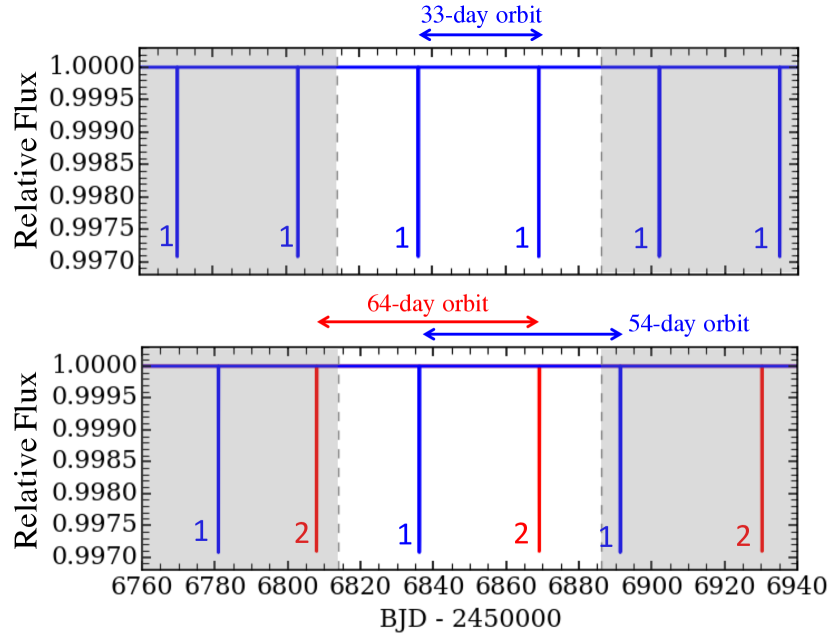
The K2 photometry, however, could not demonstrate the periodic nature of the transit signal. Instead, the 80-day K2 photometry identified only two transit events of similar depth with a separation of 33-days. Meanwhile, radial velocity confirmation of the 33-day period is currently not available because the host star is faint at visible wavelengths ($V=13.5)$ and the expected semi-amplitude of a 33-day-period planet would only be $K_{S}=1-2\,\mbox{m/s}$. As a result, the available observations leave open the alternative scenario that the two detected transit events on 2014-June-27 and 2014-July-30 were caused by two similarly-sized, long-period planets ($\gtrsim 50$ days) that happen to transit only once within the 80 days observation in K2 Campaign 1 (Figure 1). In this two-planet scenario, a planet with a 33-day orbital period and Earth-like incident stellar irradiance ($S_{inc}\approx S_{\oplus}$) would not exist around the star K2-18. We find that two-planet scenarios can lead to equally good fits to the long-cadence K2 data because the increase in transit duration with orbital period can effectively be compensated by a high impact parameter and/or an eccentric orbit.

To distinguish between the one and two planet scenario, we obtained Spitzer high precision photometry at $4.5\,\mu m$ to probe for a third transit event that would only occur if a habitable-zone super-Earth indeed existed in a 33-day orbit around K2-18. A detection of a third transit at the predicted time would prove the periodic nature of the signal. It would simultaneously also rule out potential scenarios in which one or both of the identified transit-like events were the result of residual systematic effects in the corrected K2 photometry. Such scenarios are conceivable because the detected signals are well below the noise floor of the uncorrected K2 photometry and outliers well above the median light curve scatter are common in the corrected K2 photometry despite state-of-the-art detrending (e.g., Vanderburg & Johnson, 2014; Foreman-Mackey et al., 2015).

The article is structured as follows: In Section 2, we describe the Spitzer and K2 observations used in this work as well as our photometric extraction routines. Section 3 presents the light curves analyses. Finally, we discuss the results and conclusions in Section 4.

Figure 1.— Plausible scenarios in agreement with the available K2 data of K2-18. The white region indicates the time span observed by K2. The two detected transit events at $\mathrm{BJD=2,456,836}$ and $\mathrm{BJD=2,456,869}$ can be fit equally well by a single planet in a 33-day orbit at low impact parameter (top panel) or two long-period planets at slightly higher impact parameter (bottom panel).

Figure 2.— Photometric scatter versus the width of the binning interval for Spitzer data of K2-18b. The root-mean-square error of the systematics-corrected Spitzer data (blue points) follows closely the theoretical square-root scaling for uncorrelated white noise (black line). The left-most data point corresponds to the unbinned 2-second exposures.

Figure 3.— Light curve fit to the Spitzer transit observation of K2-18b. The top panel shows the best fitting model light curve (blue), overlaid with the systematics-corrected Spitzer data. The transit of K2-18b appears $7\sigma$ (1.85 hours) before the predicted transit time from Montet et al. 2015 (vertical black line). Residuals from the light curve fitting are plotted in the middle panel, with uncertainty bars corresponding to the fitted photometric scatter. The final systematics-corrected photometry is near the Poisson noise limit and virtually free of red noise and systematics. For clarity, Spitzer data are binned to 10-minute intervals. The bottom panel shows the raw Spitzer photometry (blue), overlaid with the model fit (red). Only Spitzer observations are used in this fit.

2. Observations

2.1. Spitzer/IRAC

We observed the star K2-18 (EPIC 201912552) for a total of 8.1 hours on August 29, 2015 to search for the predicted transit of the super-Earth candidate K2-18b as part of our K2 follow-up program (GO 11026, PI Werner, see also Beichman et al. 2016). The science observation began three hours before the start of the predicted transit of K2-18b and ended two hours after the end of the predicted transit to account for transit ephemeris uncertainties and to provide adequate baselines on either side of the transit. An additional 30-minute of pre-observation (not used in the analysis) preceded the science observation to mitigate the initial instrument drift in the science observations resulting from telescope temperature changes after slewing from the preceding target (Grillmair et al., 2012). Both pre-observation and science observations were taken using Spitzer/IRAC Channel 2 in stare mode. To enhance the accuracy in positioning the target star K2-18 on the IRAC detector, the pre-observations were taken in peak-up mode using the Pointing Calibration and Reference Sensor (PCRS) as a positional reference.

We chose Spitzer/IRAC Channel 2 ($4.5\,\mathrm{\mu m}$) because the instrumental systematic due to intra-pixel sensitivity variations are smaller for Channel 2 than for Channel 1 (Ingalls et al., 2012). Our exposure times were set to 2 seconds to optimize the integration efficiency while comfortably remaining in the linear regime of the IRAC detector. Subarray mode was used to reduce the readout overhead and lower the data volume for the downlink. In total, our science data are composed of 13,632 individual frames forming a 7.6-hour broadband photometric time series of K2-18 at $4.5\,\mathrm{\mu m}$.

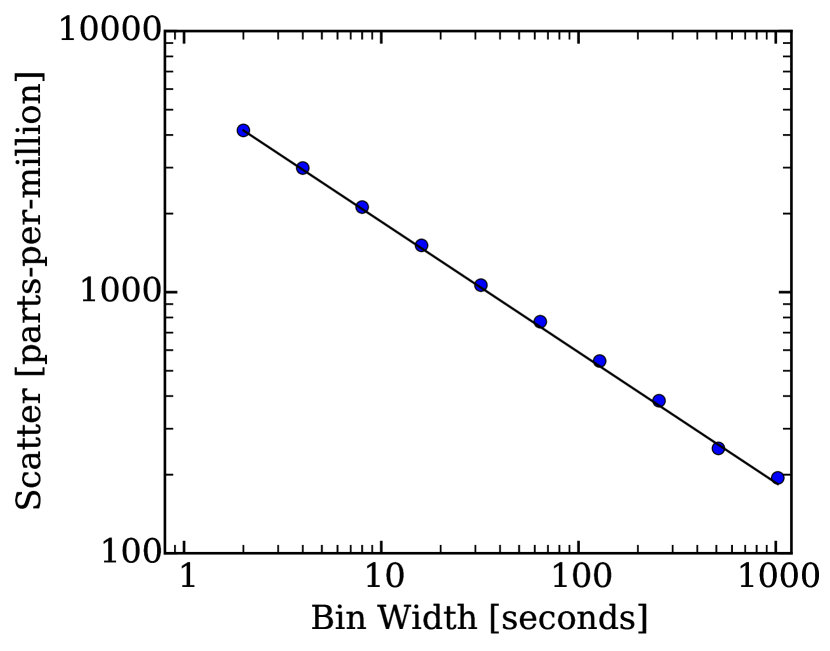
We extract multiple photometric light curves from the science data using a wide range of fixed and variable aperture sizes. The purpose of extracting and comparing multiple photometric light curves is to choose the aperture that provides the lowest residual scatter and red-noise component. For each aperture, our extraction includes estimating and subtracting the sky background, calculating the flux-weighted centroid position of the star on the array, and then calculating the total flux within circular apertures (Knutson et al., 2012; Lewis et al., 2013; Todorov et al., 2013; Kammer et al., 2015). For the fixed apertures we consider radii between 2.0 and 5.0 pixels. For the time varying apertures, we first calculate the scaling of the noise pixel parameter $\beta=(\sum_{n}I_{n})^{2}/(\sum_{n}I_{n}^{2})$, where $I_{n}$ is the measured intensity in the $n$-th pixel (Mighell, 2005), and then iteratively rescale the noise pixel aperture radius as $r=a\sqrt{\beta}+c,$ where we explore values between 0.6 and 1.2 for the scaling factors $a$ and values between 0.6 and 1.2 for the constant c. We choose this range for a and c because we noted in previous Spitzer work that the photometric scatter increases outside this range (Kammer et al., 2015). Finally, we pick the version of the Spitzer photometry with the lowest red-noise component. Our red-noise measure is the summed square difference between the noise scaling obtained by successively doubling the bin size and the theoretical square-root noise scaling for a Poisson process (Figure 2). In our case, the version of the photometry with the lowest red-noise also results in the lowest RMS.

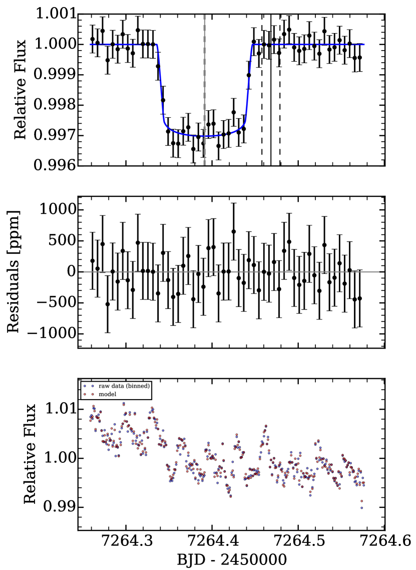
Our analysis is performed on the entire 7.6-hour science data since there is no evidence for a residual ramp effect at the beginning of the science data. We normalize the light curve by the median value and bin the data to 60-second cadence. We find that moderate binning to 60 seconds does not affect the information content of the photometry, but provides more signal per data point allowing an improved correction of the systematics (Section 3). We calculate $\mathrm{BJD_{UTC}}$ mid-exposure times using the information in the header of the BCD files provided by the Spitzer pipeline. We show the resulting uncorrected light curve for the fixed aperture with a radius of 3.0 pixels in Figure 3 (bottom panel).

2.2. K2 Photometry

The star K2-18 was observed by the Kepler Space Telescope as part of K2 Campaign 1 covering an 80-day time span between November 14, 2014 and February 3, 2015. We extract the K2 photometry directly from the Kepler pixel data downloaded from the Mikulski Archive for Space Telescopes (MAST). The star is listed as EPIC-201912552. The full data set is a time series composed of 3737 individual 16x16 pixel images centered on the star K2-18. The individual images have a cadence of 29.4 minutes and were obtained by co-adding 270 exposures (each 6.02 seconds plus 0.52 seconds readout) onboard the Kepler spacecraft (Gilliland et al., 2010). We do not do any additional time binning during the photometric extraction and light curve analysis of the K2 data.

2.2.1 Photometric Extraction

Our photometric extraction routine is outlined in Crossfield et al. (2015) and Petigura et al. (2015), following the approach introduced by Vanderburg & Johnson (2014). In brief, during the continuous 80-day K2 observations, the stars drift across the CCD by approximately 1 pixel every 6 hours due to the spacecraft’s pointing jitter. As the stars drift through pixel-phase, intra-pixel sensitivity variations and errors in the flatfield cause the apparent brightness of the target star to change. We detrend the apparent brightness variations of our target using the telescope roll angle between the target frame and an arbitrary reference observation. For each of the two transits, we then extract transit light curves ranging from three hours before the transit ingress to three hours after ingress, providing sufficient baseline for the transit light curve analysis.

2.2.2 A Cosmic Ray Detection Algorithm for K2 Photometry

Figure 4.— Cosmic ray detection for K2 photometry. Panel (a) shows the background subtracted image of K2-18b for the observation affected by a cosmic-ray hit (red data point in Figure 7). Panel (c) shows the same frame after subtracting the “most similar frame” in the K2 time series of K2-18b (Panel (b)). The cosmic hit is clearly identified in the difference image near x=4.5 and y=5.5. For comparison, Panel (d) shows an equivalent difference image for an observation not affected by a cosmic ray hit. Small residuals remain near the center of the PSF, but are not mistaken as cosmic ray hits by our new cosmic ray detection algorithm (Section 2.2.2)

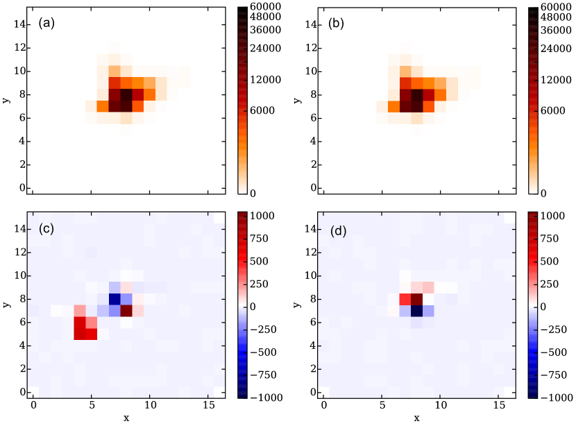
As shown in this work, cosmic ray hits can substantially affect the astrophysical results derived from K2 photometry. This is particular troubling because the effects of cosmic ray hits are generally too small to result in obvious outliers in the long-cadence, 30-minute K2 photometry. As a result, cosmic ray hits have stayed unnoticed to date, and at least for K2-18b have resulted in inaccurate estimates of the transit parameters. To address this issue and detect cosmic ray hits in the K2 photometry, we introduce a generally applicable algorithm to efficiently identify cosmic ray hits in the presence of substantial telescope jitter as we see for K2.

We apply the algorithm to the K2-18 data as follows. First, we remove the sky background from each individual frame by subtracting the median pixel value outside the PSF of the target star. For each background-subtracted frame in the K2 image series, we then find a “most similar frame” by identifying the frame in the K2 image series that minimizes the weighted sum of the square differences in x and y centroid location and telescope roll angle. This most similar frame will generally appear virtually identical to the original frame because the PSF falls virtually identical on the detector pixels. The most similar frame can, therefore, be used to subtract the target star from the image and isolate potential cosmic ray hits. Finally. we automatically identify cosmic ray hits by searching for $>10\sigma$ outliers in the time series of each pixel in the difference images.

As an example, Figure 4 shows the detection of the cosmic ray hit near the ingress of the second K2 transit observation of K2-18b. Panel (a) shows the background subtracted image of K2-18b for the cosmic-ray affected observation near the ingress of the second transit. For comparison, panel (b) shows the frame in the K2-18 data with the most similar centroid position (BJD=2456875.66). Panels (a) and (b) appear virtually identical despite the strong color stretching. The cosmic ray hit near x=4.5 and y=5.5 becomes apparent, however, in the difference image (Panel (c)). The five pixels near the cosmic ray hit are identified as outliers with a significance of $>20\sigma$ in the difference image light curves for these pixels. For comparison, Panel (d) shows the difference image for a regular frame without cosmic ray hit. Small residuals ($\sim 1\%$) in the difference image remain due to slight differences in the centroid position and shape of the PSF. However, the residuals are not mistaken as cosmic ray hits because the pixel values are within the variances of the difference image light curves for those pixels.

2.3. Stellar Spectroscopy

Figure 5.— Calibrated IRTF/SpeX JHK-band spectrum of K2-18 compared to late-type standards from the IRTF Spectral Library. The spectra are normalize to the continuum in each band. Across the three bands, the continuum shape and the strengths of individual absorption features are most consistent with the M2/M3 standards. This is consistent with the $\mathrm{M2.5\pm 0.5}$ spectral type estimated using index based methods. Spectroscopically derived stellar parameters are listed in Table 2.

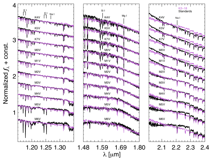
We observed K2-18 using the near-infrared cross-dispersed spectrograph (SpeX) on the NASA Infrared Telescope Facility (IRTF) to independently verify its metallicity ([Fe/H]), effective temperature ($T_{\mathrm{eff,*}}$), radius ($R_{*}$), mass ($M_{*}$), and luminosity ($L_{*}$). Following the procedure described in Crossfield et al. (2015), Petigura et al. (2015), and Schlieder et al. (2016), we obtain stellar properties that are consistent with the stellar properties reported by Montet et al. (2015) (Table 2). In short, we observed K2-18 using the short cross-dispersed mode and 0.3x15” slit providing simultaneous wavelength coverage from 0.68 to $2.5\,\mathrm{\mu m}$ at a resolution of $R=2000$ (Figure 5). The median SNR of our SpeX spectrum is 145 across the JHK bands. Based on the SpeX spectrum, we estimate the stellar metallicity using empirical methods based on the spectroscopic indices and equivalent widths calibrated using M dwarfs that have wide, co-moving FGK companions with well determined [Fe/H] (Boyajian et al., 2012; Mann et al., 2013a). Similarly, we extract the effective temperature using temperature sensitive spectroscopic indices in the JHK-bands (Mann et al., 2013b) and empirical relations calibrated using nearby, bright M dwarfs (Boyajian et al., 2012). We also estimate the spectral type of K2-18 from our SpeX spectrum using the molecular index based methods of Lépine et al. (2013) ($\mathrm{TiO_{5}}$, $\mathrm{CaH_{3}}$) and Rojas-Ayala et al. (2012) ($\mathrm{H_{2}O-K_{2}}$). Both methods provide a spectral type of $\mathrm{M2.5\pm 0.5}$. This type is consistent with the derived stellar parameters and a visual comparison to late-type standards from the IRTF Spectral Library (Figure 5, Rayner et al. (2009); Cushing et al. (2005)). Finally, we combine the derived $T_{\mathrm{eff,*}}$ and [Fe/H] and compute the stellar radius and luminosity using the empirical $T_{\mathrm{eff}}$-[Fe/H]-$R_{*}$ relation provided by Mann et al. (2015).

3. Light Curve Analyses

3.1. Spitzer Confirmation of K2-18b

Figure 6.— Pairs plot showing the posterior distribution of the MCMC fitting parameters for the Spitzer light curve fit. The panels on the diagonal show the marginalized posterior distribution for each fitting parameter. The 68% credible interval is marked by vertical dashed lines and quantified above the panel. The off-diagonal panels show the two-dimensional marginalized distribution for pairs of parameters, with the gray shading corresponding to the probability density and black contours indicating the 68% and 95% credible regions. Using our modified PLD-based Spitzer instrument model, we find that the posterior distributions of all fitting parameters are near-Gaussian, and that the astrophysical parameters ($R_{P}/R_{*}$, $T_{C}$, $b$) are virtually uncorrelated with our instrumental parameters ($w_{1}\ldots w_{9},\,m,\,\sigma_{0}$). The inset at the top right shows a typical image of K2-18’s on the Spitzer/IRAC detector, labeling the 3x3 pixels covering the central region of the PSF.

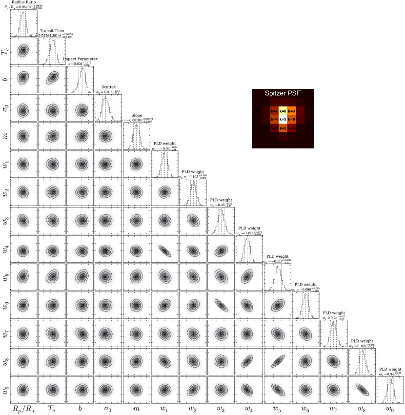
We analyze the Spitzer raw photometry by simultaneously fitting our Spitzer/IRAC instrument model, a transit light curve model, and a photometric scatter parameter using Markov Chain Monte Carlo. The entire analysis from raw photometry to the transit parameters and their uncertainties is performed as a one-step, statistically consistent Bayesian analysis.

3.1.1 Spitzer/IRAC Instrument Model

Our Spitzer/IRAC instrument model accounts for intrapixel sensitivity variations and temporal sensitivity changes using a modified version of the systematics model proposed by Deming et al. (2015). Our instrument model is

$$S\left(t_{i}\right)=\frac{\sum_{k=1}^{9}w_{k}D_{k}\left(t_{i}\right)}{\sum_{k=1}^{9}D_{k}\left(t_{i}\right)}+m\cdot t_{i},$$ (1)

where the sensitivity function $S\left(t_{i}\right)$ is composed of the pixel-level decorrelation (PLD) term introduced by Deming et al. (2015) and a linear sensitivity gradient in time. The $D_{k}\left(t_{i}\right)$’s in the PLD term are the raw counts in the 3x3 pixels, $k=1\ldots 9$, covering the central region of the PSF. In the numerator, these raw data values are multiplied by the nine time-independent PLD weights, $\left\{w_{1}\ldots w_{9}\right\}$, fitted as free parameters in the light curve analysis. Together with the linear slope $m$, the instrument model therefore includes 10 free instrument fitting parameters to capture the intrapixel sensitivity variations and temporal sensitivity changes. The differences between Equation 1 in this work and Equation 4 in Deming et al. (2015) are that we do not include the offset constant ($h$) and we apply $S\left(t_{i}\right)$ as a multiplicative correction factor corresponding to a variation in sensitivity rather than an additive term. The log-likelihood function for fitting the Spitzer raw photometry is then

$$\log L=-\frac{1}{2}\sum_{i=1}^{N}\left(\frac{D\left(t_{i}\right)-S\left(t_{i}\right)\cdot f\left(t_{i}\right)}{\sigma}\right)^{2},$$ (2)

where $f\left(t_{i}\right)$ is the median-normalized flux summed over all pixels of the target’s PSF, $S\left(t_{i}\right)$ is aforementioned instrument sensitivity, $f\left(t_{i}\right)$ is the model transit light curve, and $\sigma$ is the photometric scatter parameter simultaneously fit with the instrument model and transit light curve parameters.

We do not include the constant term $h$ from Deming et al. (2015) because only the relative sizes of the PLD weights carry information about the intrapixel sensitivity variation. The sum of the PLD weights $\sum_{k}w_{k}$ uniformly scales the entire light curve up or down, which is perfectly equivalent to adding a constant $h$. As a result, if an extra term $h$ was included, it would be perfectly degenerate with $\sum_{k}w_{k}$ in the fitting, resulting in 100% degeneracies between the nine PLD weight and $h$.

We choose to include $S\left(t_{i}\right)$ as a multiplicative correction factor rather than an additive term as done by Deming et al. (2015) because the multiplicative factor matches more closely the underlying detector behavior, which is a variation in sensitivity (or quantum efficiency) across the pixel area. The difference between a multiplicative factor and a additive term is generally small because $S\left(t_{i}\right)$ is near unity and the multiplication can be approximated by $1+\epsilon$. However, the inaccuracy due to the negligence of the cross-term $\delta f\cdot\delta S$ can be as high as $0.01\cdot 0.005=50\,\textrm{parts-per-million}$ for 1% transit depth and typical sensitivity variations. We choose to be on the safe side by introducing a multiplicative correction factor that correctly captures the cross-term $\delta f\cdot\delta S$.

3.1.2 Transit Model

Figure 7.— Joint light curve fit to the K2 and Spitzer observation of K2-18b. The top panels shows the best fitting model light curve (blue line), overlaid with the systematics-corrected K2 data (left and middle) and Spitzer data (right). Residuals from the light curve fitting are plotted in the bottom panels, with vertical bars corresponding to the fitted photometric scatter. An outlier data point affected by a cosmic ray hit near the ingress of the second K2 transit is indicated in red and ignored in the light curve fitting (see also Section 2.2.2). The high-cadence Spitzer data critically helped identifying the outlier by precisely constraining the transit duration and transit impact parameter.

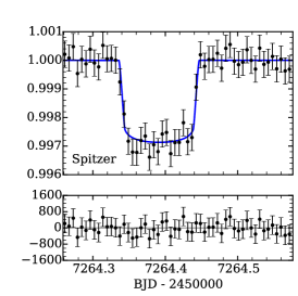
We compute the transit light curve $f\left(t_{i}\right)$ using the Batman implementation (Kreidberg, 2015) of the Equations derived in Mandel & Agol (2002). The transit parameters fitted in our Spitzer analysis are the planet-to-star radius ratio $R_{P}/R_{*}$, the mid-transit time $T_{C}$, and the impact parameter $b$. We fix the stellar radius and mass to the values derived based on stellar spectroscopy (Table 2) and assume a circular orbit. We use a quadratic limb darkening profile with coefficients interpolated from the tables provided by Claret & Bloemen (2011) for K2-18’s stellar effective temperature and surface gravity ($u_{1}=0.007\pm 0.007$, $u_{2}=-0.191\pm 0.005$). These limb darkening coefficients are computed specifically for the $4.5\,\mathrm{\mu m}$ Spitzer/IRAC Channel 2 bandpass from spherically symmetric Phoenix models (e.g., Hauschildt et al., 1999) using updated opacities. We account for the $\sim$30 minute cadence of the K2 observations by numerically integrating in time.

3.1.3 MCMC Analysis

We compute the joint posterior distribution of the instrument and transit parameters using the emcee package (Foreman-Mackey et al., 2013), a Python implementation of the Affine Invariant Markov Chain Monte Carlo (MCMC) Ensemble sampler (Goodman & Weare, 2010). We seed 60 MCMC walkers with initial values widely spread in the prior parameter space. For convergence, we ensure that the chains for all parameters are well-mixed as indicated by Gelman-Rubin metrics smaller than 1.02 (Gelman & Rubin, 1992). After an initial burn-in phase, we generally find good convergence after 3000 to 4000 iterations for each of the 60 walkers. Since the computational time is not a limiting factor in this work, we quadruple the number of iterations to obtain smooth posterior distributions (Figure 6). The final confidence intervals reported in this work are the 15.87% and 84.13% percentiles of each parameters’ posterior distribution.

3.1.4 Spitzer Results

Our Spitzer observations robustly reveal a transit event consistent in transit depth and duration with the super-Earth candidate K2-18b. The transit event, however, occurs approximately 1.85 hours ($7-\sigma$) before the transit time predicted for K2-18b by Montet et al. (2015), which will be discussed further in the following section.

We also find that, using our new modified PLD systematics model, the final systematics-corrected photometry is near the photon-noise limit and virtually free of red noise and systematics (Figures 2 and 3). All posteriors of Spitzer/IRAC systematics parameters are Gaussian-shaped and uncorrelated with the astrophysical parameters in the transit model, indicating that there is no dependency of the astrophysical parameters on the instrument parameters (Figure 6).

3.2. Joint Spitzer/K2 Analysis

To investigate the source of the $7\,\sigma$ discrepancy between the predicted and measured transit times, we perform a global analyses of the Spitzer and K2 data. We directly determine the transit parameters and their uncertainties from the K2 and Spitzer raw photometries by simultaneously fitting the transit light curve model, our Spitzer/IRAC instrument model, and linear drifts in the photometry of the K2 transits. We further assume in this Section 3.2 that K2-18b is orbiting its host star in a Keplerian orbit with a periodic transit ephemeris and that the transit depths at visible wavelength (K2) and IR wavelength (Spitzer) are identical. These assumptions are relaxed in Sections 3.3 and 3.4 and found to be appropriate.

3.2.1 Instrument Models

Since we fit the Spitzer photometry and two K2 transits simultaneously, our fit now includes 14 free parameters for instrument systematics. As in Section 3.1, we include nine PLD weights and one linear slope to account for the intrapixel sensitivity variations and temporal sensitivity changes in the Spitzer photometry (Section 3.1.1). In addition, two free parameters are included for each of the two K2 transits to account for the linear slope and offset in the K2 baseline. The log-likelihood function for simultaneously fitting the Spitzer transit and the two K2 transits is

$$\begin{split}\log L=-\frac{1}{2}\sum_{i=1}^{N_{\mathrm{S}}}\left(\frac{D_{\mathrm{Spitzer}}\left(t_{i}\right)-S\left(t_{i}\right)\cdot f\left(t_{i}\right)}{\sigma_{\mathrm{Spitzer}}}\right)^{2}\\ -\frac{1}{2}\sum_{i=1}^{N_{1}}\left(\frac{D_{\mathrm{K2,1}}\left(t_{i}\right)-\left(m_{1}t_{i}+b_{1}\right)\cdot f\left(t_{i}\right)}{\sigma_{\mathrm{K2}}}\right)^{2}\\ -\frac{1}{2}\sum_{i=1}^{N_{2}}\left(\frac{D_{\mathrm{K2,2}}\left(t_{i}\right)-\left(m_{2}t_{i}+b_{2}\right)\cdot f\left(t_{i}\right)}{\sigma_{\mathrm{K2}}}\right)^{2},\end{split}$$ (3)

where $\sigma_{\mathrm{Spitzer}}$ and $\sigma_{\mathrm{K2}}$ are the fitted photometric scatter values for the Spitzer and K2 photometry, $N_{s}$, $N_{1}$, and $N_{2}$ are the number of data points for each of the transit light curves, and $mt_{i}+b$ is the linear baseline for the individual K2 transit light curves.

Parameter	Spitzer only	Spitzer + K2	Spitzer + K2	Spitzer + K2	Unit
	Keplerian orbit	Keplerian orbit	Transit timing	Transit depth comp.
	(Section 3.1)	(Section 3.2)	(Section 3.3)	(Section 3.4)
Radius ratio $R_{P}/R_{*}$	$0.05397_{-0.00089}^{+0.00085}$	$0.05295_{-0.00059}^{+0.00061}$	$0.05303_{-0.00059}^{+0.00059}$	$0.05205_{-0.00076}^{+0.00077}$ (Kepler)	1
				$0.05391_{-0.00088}^{+0.00082}$ (Spitzer)
Impact parameter, $b$	$0.604_{-0.014}^{+0.012}$	$0.601_{-0.011}^{+0.013}$	$0.603_{-0.011}^{+0.011}$	$0.601_{-0.011}^{+0.012}$	1
Ephemeris:
Mid-transit time, $T_{C}$	$2457264.39144_{-0.00066}^{+0.00059}$	$2457264.39131_{-0.00067}^{+0.00060}$		$2457264.39135_{-0.00066}^{+0.00062}$	BJD
Orbital period, $P$	32.94 (fixed)	$32.939614_{-0.000084}^{+0.000101}$		$32.939622_{-0.000094}^{+0.000099}$	days
Individual transit times:
K2 Transit 1			$2456836.1767_{-0.0026}^{+0.0008}$		BJD
K2 Transit 2			$2456869.11526_{-0.00080}^{+0.00076}$		BJD
Spitzer			$2457264.39141_{-0.00063}^{+0.00059}$		BJD

Table 1Transit parameters derived from the Spitzer and K2 light curves of K2-18b.

Param		Units	K2-18b
$T_{0}$		BJD	$2457264.39144_{-0.00066}^{+0.00059}$
$P$		d	$32.939614_{-0.000084}^{+0.000101}$
$b$		$-$	$0.601_{-0.011}^{+0.013}$
$R_{\mathrm{P}}/R_{*}$		$\%$	$5.295_{-0.059}^{+0.061}$
$a$		AU	$0.1429_{-0.0065}^{+0.0060}$
$i$		deg	$89.5785_{-0.0088}^{+0.0079}$
$R_{\mathrm{P}}$		$R_{\oplus}$	$2.279_{-0.025}^{+0.026}$
$S_{\mathrm{inc}}$		W	$1432_{-270}^{+293}$
$S_{\mathrm{inc}}$		$S_{\oplus}$	$1.05_{-0.20}^{+0.22}$
$T_{14}$		min	$159.78_{-1.62}^{+1.40}$
$T_{23}$		min	$135.24_{-1.96}^{+1.74}$
$R_{*}$		$R_{\odot}$	$0.411\pm 0.038$
$M_{*}$		$M_{\odot}$	$0.359\pm 0.047$
$T_{\mathrm{eff,*}}$		K	$3457\pm 39$
[Fe/H]		(dex)	$0.123\pm 0.157$
$\rho_{\mathrm{*,spec}}$		$\mathrm{g\,cm^{-3}}$	$7.87\pm 1.26$

Table 2Summary of planet and host star properties.

3.2.2 Transit Model

Our global light curve fit includes a wavelength-independent planet-to-star radius ratio $p=R_{P}/R_{*}$, the impact parameter $b$, the mid-transit time $T_{C}$ , and the orbital period $P$. As in Section 3.1.2, we fix the stellar radius and stellar mass to the values derived based on stellar spectroscopy (Table 2) and assume a circular orbit. For the $4.5\,\mathrm{\mu m}$ Spitzer/IRAC Channel 2 observations, we use the same quadratic limb darkening profile ($u_{1}=0.007\pm 0.007$, $u_{2}=-0.191\pm 0.005$) as in Section 3.1.2. For the visible Kepler bandpass, we derive the quadratic limb darkening coefficients ourselves using Phoenix models and obtain $u_{1}=0.153\pm 0.004$ and $u_{2}=0.261\pm 0.007$.

3.2.3 Spitzer/K2 Results

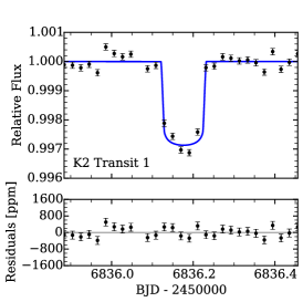
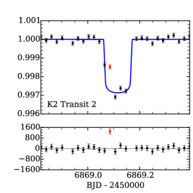
Our joint analysis of the Spitzer and K2 data reveals that a previously undetected outlier point in the K2 photometry near the ingress of second K2 transit is the reason for the 1.85 hours ($7\,\sigma$) discrepancy between the transit time predicted from the K2 data and the transit time observed by Spitzer (Figure 7). Using our newly developed cosmic ray detection algorithm we find that the outlier is caused by a cosmic ray hit near the edge of the target star’s PSF on the detector (Figure 4). After removal of the outlier point, we find that a Keplerian orbit with periodic transit events provide a good joint fit to the K2 and Spitzer transit light curves (Figure 7). Our new best estimate for the transit ephemeris of K2-18b is $T_{0}=2457264.39131_{-0.00067}^{+0.00060}$ and $P=32.939614_{-0.000084}^{+0.000101}$.

As for the Spitzer-only fit in Section 3.1.4, we find that the posteriors of all transit light parameters are Gaussian-shaped and uncorrelated with the parameters in the systematics model. This indicates that the derived astrophysical parameters are independent of the fitted instrument parameters in our joint Spitzer/K2 fit. We further find that including the K2 in the fit does not compromise the excellent noise characteristic of the fit to the Spitzer data (compare Figure 3 and 7(right panel)).

3.3. Individual Transit Times

Figure 8.— Transit times of K2-18b relative to the best-fitting linear ephemris extracted from the global fits to the K2 and Spitzer data. After removing the outlier in the K2 photometry, the data of K2-18b are well explained by Keplerian orbit with linear ephemeris.

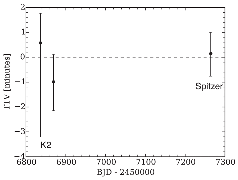
We perform a second global fit to the K2 and Spitzer data to demonstrate that the initial 1.85 hours discrepancy between the transit time observed by Spitzer (Section 3.1) and the expected transit time based on Montet al. 2015 is well explained by the previously undetected cosmic ray hit in the K2 data. Our transit timing analysis is identical to the analysis presented in Section 3.2 except that we do not fit for an average orbital period, but instead parameterize the mid-transit times of all three individual transits individually (Table 1) We remove the discrepant data point near the ingress of the second K2 transit (Figure 7). Finally, we probe for deviations from a linear ephemeris derived in Section 3.2 by plotting the differences between the individually fitted transit times and the calculated transit times from the best-fitting linear transit ephemeris (Figure 8).

We find that all three measured transit times are fully consistent with a linear ephemeris to within the timing uncertainties of $1-3$ minutes. We conclude that the K2 and Spitzer data are well explained by a single planet in a Keplerian orbit. Future transit observations will be needed to rule transit timing variations below the $1-3$ minute level or with periods several times greater than the $430$ days covered by the K2 and Spitzer observations analyzed here.

3.4. Transit Depth Comparison between K2 and Spitzer

Figure 9.— Marginalized posterior distributions of the transit depths in the visible-light K2 bandpass ($0.4-0.7\,\mathrm{\mu m}$, blue) and in the infrared Spitzer/IRAC Channel 2 bandpass ($4-5\,\mathrm{\mu m}$, red). The fitted transit depths from the Spitzer and K2 data are consistent to within approximately $1-\sigma$.

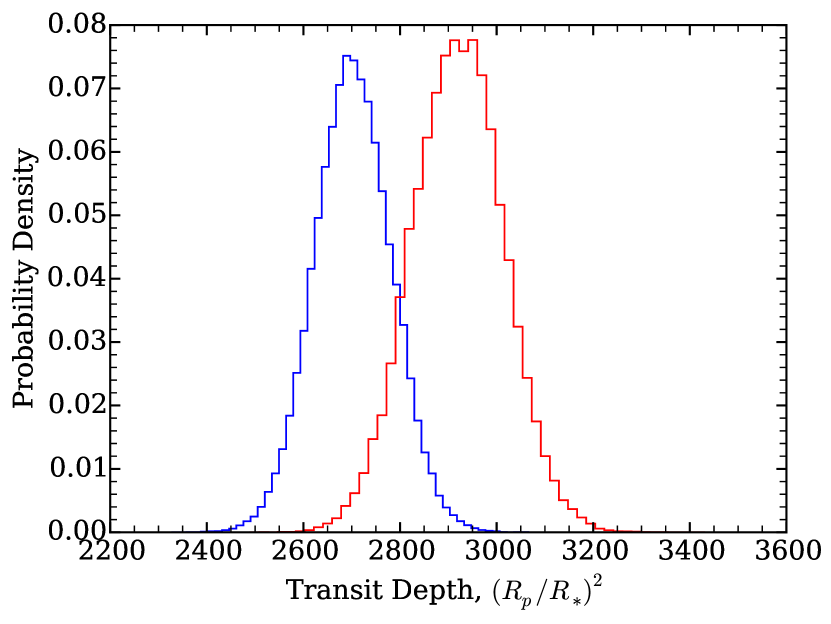
We perform a third global analysis of the K2 and Spitzer light curves to compare the transit depths in the visible-light K2 bandpass ($0.4-0.7\,\mathrm{\mu m}$) and the infrared Spitzer/IRAC bandpass ($4-5\,\mathrm{\mu m}$). Widely different transit depths at visible and infrared wavelengths could alert us to the potential presence of a blended star that would affect the inferred planetary radius measurement (Stevenson et al., 2014) or even be the source of a false positive scenario (Désert et al., 2015). Different transit depths could also result from wavelength-dependent extinction in the atmosphere of K2-18b or the presence of an exosphere or planetary rings.

We perform the global analysis identical to the one described in Section 3.2; however, this time we allow for different transit depths to fit the K2 and Spitzer transit observations (Table 1). We find that the transit depths at visible-light and infrared are consistent to within the $1\,\sigma$ uncertainties (Figure 9), ruling out any blended stars or planetary rings that would affect the transit depth measurement at visible and near-infrared wavelength by more than $10\%$ (300 ppm). The precision of the transit depth measurements, however, is currently insufficient to detect gravitationally bound atmospheres.

4. Discussion and Conclusions

Figure 10.— Deviations from the updated ephemeris. The red region illustrates the deviation in the predicted mid-transit time between the K2-derived ephemeris reported by Montet et al. 2015 and our updated ephemeris based on the joint K2-Spitzer analysis (blue). Dark and light red regions correspond to 68% and 95% confidence, respectively. Equivalently the blue regions (within the line thickness) correspond to the uncertainties of the updated K2-Spitzer ephemeris. Without the immediate Spitzer follow-up, K2-18b would have been for lost for future atmospheric characterization due to the increasing deviation in the predicted transit time. For comparison, the green region indicate the transit timing uncertainty by refitting only the K2 data without the outlier data point. The ephemeris based on only K2 remains uncertain to 1-2 hours, but the bias is eliminated by removing the outlier.

The Spitzer Space Telescope observations presented in this work confirm the presence of the habitable zone super-Earth K2-18b by detecting a third transit event with a consistent transit depth near the predicted transit time. The revealed periodicity of the transit signal demonstrates that the two transit-like events observed by K2 are indeed caused by one planet in a 33-day orbit and are not two independent events caused by two similarly-sized planets in >50-day orbits. The periodicity also rules out any scenarios in which one or both of the identified transit-like events were the result of residual systematic effects in the corrected K2 photometry. The photometric confirmation of K2-18b is critical for future atmospheric studies because K2-18b is an extremely favorable habitable-zone exoplanet for transmission spectroscopy with HST and JWST.

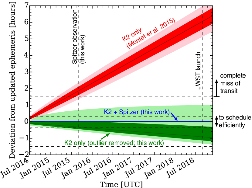
We also find, however, that the third transit event occurred 1.85 hours ($7-\sigma)$ before the predicted transit time based on the K2-derived ephemeris by Foreman-Mackey et al. (2015) and Montet et al. (2015). Our global analysis of the K2 and Spitzer data reveals that this 1.85-hour deviation is, however, not caused by TTVs from another planets in the system, but is well-explained by a single, previously undetected cosmic ray hit in the K2 photometry near the ingress of the second transit.

Our analysis of K2-18b critically reveals that transit ephemerides of long-period planets based on only two detected transit events can strongly be affected by individual outlier data points in the K2 photometry. A single outlier due to a cosmic ray hit near the ingress of the second transit biased the ephemeris of K2-18b to a level that future transit observations could have missed the transit of K2-18b completely. The deviation in the transit ephemeris would have grown to 8 hours by the time JWST launches (Figure 10). As a result, the first transiting habitable-zone planet amenable to efficient atmospheric characterization would have been lost for future spectroscopic transit observations with HST or JWST due to the increasing error in its ephemeris estimate. We conclude that immediate follow-up of prime exoplanet candidates are critical for long-period planets found by planet search missions such as K2 and TESS.

Similarly, the previously undetected outlier in the K2 photometry introduced substantial uncertainty in the inference of the planet-to-star radius ratio. After identifying the cosmic ray hit and removing the outlier we estimate the planet-to-star radius ratio to $R_{\mathrm{P}}/R_{*}=5.295\%_{-0.059\%}^{+0.061\%}$. If we ignore our knowledge about the cosmic ray hit and include the outlier data point in our analysis of the K2 light curve, we find the radius ratio uncertainty to be 9 times larger consistent with $5.13\%{}_{-0.35\%}^{+0.56\%}$ as reported by Foreman-Mackey et al. (2015). In this latter case, the wide and asymmetric uncertainties arise because the outlier data point adversely affects the overall fit to the low-cadence K2 photometry. We present an efficient search algorithm to identify cosmic ray hits in photometry data sets with substantial telescope pointing jitter to avoid similar problems in future K2 or TESS light curve analyses.

In the coming years, mass measurement of K2-18b will be critical to provide an understanding of the nature and bulk composition of K2-18b. Radial velocity measurements are challenging, however, because the host stars is faint at visible wavelengths ($V=13.5$) and the expected radial velocity semi-amplitude is small ($K_{\mathrm{P}}=1-2\,\mathrm{m/s})$. Still, thanks to the star’s brightness in the near-IR ($K=8.9$), K2-18b may present an ideal target for intensive follow-up with a number of upcoming NIR radial velocity instrument such as CARMENES (Quirrenbach et al., 2012), SPIRou (Artigau et al., 2014), IRD (Tamura et al., 2012), and CRIRES (Kaeufl et al., 2004). In addition, upcoming visible-light radial velocity instruments on large telescopes like VLT/ESPRESSO (Pepe et al., 2014), Keck/SHREK, and GMT/G-CLEF (Szentgyorgyi et al., 2012) should also be able to measure planetary mass of K2-18b in the coming years.

The infrared brightness and small stellar radius of the host star make K2-18b an extremely favorable candidate for the first detailed atmospheric characterization of a habitable-zone super-Earth. Given its radius of $2.27$$R_{\oplus}$, the planet is likely surrounded by a thick gaseous envelope (e.g., Rogers, 2015) that could be amenable to characterization through transit spectroscopy. Eventually the detectability of the K2-18b’s atmosphere will depend on the mean molecular mass of the atmosphere and presence of high-altitude clouds (Miller-Ricci et al., 2009; Benneke & Seager, 2013). In addition, the range of plausible atmospheric scenarios for K2-18b also depends on the yet unknown planetary mass and surface gravity. Little is known about the nature of planets in the habitable zone around M stars, making K2-18b a unique opportunity to probe chemical composition and formation history with future follow-up observations.

The K2 and Spitzer analyses presented in this work were performed using ExoFit, a newly-developed, Python-based light curve analysis framework. The new framework is highly modular in that it can jointly fit any number of Kepler, Spitzer, HST WFC3, and/or HST STIS transit observations in a global MCMC analysis with minimum user input. In this work, the joint analysis of Spitzer and K2 data provides substantial advantage over individual transit fits because the high cadence Spitzer observations provide exquisite constraints on thetransit duration that helps fitting the low-cadence K2 data. For the analysis of the Spitzer observations, we introduce two modifications to the pixel-level-decorrelation (PLD) approach introduced by Deming et al. (2015). We find that these changes can provide substantial advantages in the convergence and uncertainty estimation. With the modifications, the posterior distribution of all PLD weights in our analyses converge to Gaussian-shaped posteriors that are uncorrelated with the astrophysical parameters, providing confidence that the derived transit light curve parameters are independent of the instrument parameters. Critically, our corrected Spitzer light curve is virtually free of residual red noise or systematics. The photometric precision of our final Spitzer light curve is near the Poisson limit.

This work is based in part on observations made with the Spitzer Space Telescope, which is operated by the Jet Propulsion Laboratory, California Institute of Technology under a contract with NASA. Support for this work was provided by NASA through grants under the HST-GO-13665 program from the STScI and through an award issued by JPL/Caltech. A. W. H. acknowledges support for our K2 team through a NASA Astrophysics Data Analysis Program grant. A. W. H. and I. J. M. C. acknowledge support from the K2 Guest Observer Program.

Facility: Spitzer, Kepler, K2, IRTF (SpeX)

References

- Artigau et al. (2014) Artigau, É., et al. 2014, in , 914715–914715–13
- Beichman et al. (2016) Beichman, C., et al. 2016, ApJ, 822, 39
- Benneke & Seager (2013) Benneke, B., & Seager, S. 2013, ApJ, 778, 153
- Boyajian et al. (2012) Boyajian, T. S., et al. 2012, ApJ, 757, 112
- Burke et al. (2015) Burke, C. J., et al. 2015, ApJ, 809, 8
- Claret & Bloemen (2011) Claret, A., & Bloemen, S. 2011, A&A, 529, A75
- Crossfield et al. (2015) Crossfield, I. J. M., et al. 2015, ApJ, 804, 10
- Cushing et al. (2005) Cushing, M. C., Rayner, J. T., & Vacca, W. D. 2005, The Astrophysical Journal, 623, 1115
- Deming et al. (2015) Deming, D., et al. 2015, ApJ, 805, 132
- Désert et al. (2015) Désert, J.-M., et al. 2015, ApJ, 804, 59
- Farr et al. (2015) Farr, W. M., Gair, J. R., Mandel, I., & Cutler, C. 2015, Physical Review D, 91, 023005
- Foreman-Mackey et al. (2013) Foreman-Mackey, D., Hogg, D. W., Lang, D., & Goodman, J. 2013, Publications of the Astronomical Society of the Pacific, 125, 306
- Foreman-Mackey et al. (2014) Foreman-Mackey, D., Hogg, D. W., & Morton, T. D. 2014, The Astrophysical Journal, 795, 64
- Foreman-Mackey et al. (2015) Foreman-Mackey, D., Montet, B. T., Hogg, D. W., Morton, T. D., Wang, D., & Schölkopf, B. 2015, ApJ, 806, 215
- Gelman & Rubin (1992) Gelman, A., & Rubin, D. B. 1992, Statistical Science, 7, 457
- Gilliland et al. (2010) Gilliland, R. L., et al. 2010, ApJ, 713, L160
- Goodman & Weare (2010) Goodman, J., & Weare, J. 2010, Communications in Applied Mathematics and Computational Science, 5, 65
- Grillmair et al. (2012) Grillmair, C. J., et al. 2012, in Society of Photo-Optical Instrumentation Engineers (SPIE) Conference Series, Vol. 8448
- Hauschildt et al. (1999) Hauschildt, P. H., Allard, F., & Baron, E. 1999, The Astrophysical Journal, 512, 377
- Ingalls et al. (2012) Ingalls, J. G., Krick, J. E., Carey, S. J., Laine, S., Surace, J. A., Glaccum, W. J., Grillmair, C. C., & Lowrance, P. J. 2012 (International Society for Optics and Photonics), 84421Y–84421Y–13
- Kaeufl et al. (2004) Kaeufl, H.-U., et al. 2004, in , 1218–1227
- Kammer et al. (2015) Kammer, J. A., et al. 2015, ApJ, 810, 118
- Knutson et al. (2012) Knutson, H. A., et al. 2012, ApJ, 754, 22
- Kreidberg (2015) Kreidberg, L. 2015
- Lépine et al. (2013) Lépine, S., Hilton, E. J., Mann, A. W., Wilde, M., Rojas-Ayala, B., Cruz, K. L., & Gaidos, E. 2013, The Astronomical Journal, 145, 102
- Lewis et al. (2013) Lewis, N. K., et al. 2013, The Astrophysical Journal, 766, 95
- Mandel & Agol (2002) Mandel, K., & Agol, E. 2002, ApJ, 580, L171
- Mann et al. (2013a) Mann, A. W., Brewer, J. M., Gaidos, E., Lépine, S., & Hilton, E. J. 2013a, The Astronomical Journal, 145, 52
- Mann et al. (2015) Mann, A. W., Feiden, G. A., Gaidos, E., Boyajian, T., & Braun, K. v. 2015, ApJ, 804, 64
- Mann et al. (2013b) Mann, A. W., Gaidos, E., & Ansdell, M. 2013b, ApJ, 779, 188
- Mighell (2005) Mighell, K. J. 2005, MNRAS, 361, 861
- Miller-Ricci et al. (2009) Miller-Ricci, E., Seager, S., & Sasselov, D. 2009, ApJ, 690, 1056
- Montet et al. (2015) Montet, B. T., et al. 2015, ApJ, 809, 25
- Pepe et al. (2014) Pepe, F., et al. 2014, Astron. Nachr., 335, 8
- Petigura et al. (2013) Petigura, E. A., Marcy, G. W., & Howard, A. W. 2013, ApJ, 770, 69
- Petigura et al. (2015) Petigura, E. A., et al. 2015, ApJ, 811, 102
- Quirrenbach et al. (2012) Quirrenbach, A., et al. 2012, in , 84460R–84460R–13
- Rayner et al. (2009) Rayner, J. T., Cushing, M. C., & Vacca, W. D. 2009, ApJS, 185, 289
- Rogers (2015) Rogers, L. A. 2015, ApJ, 801, 41
- Rojas-Ayala et al. (2012) Rojas-Ayala, B., Covey, K. R., Muirhead, P. S., & Lloyd, J. P. 2012, ApJ, 748, 93
- Schlieder et al. (2016) Schlieder, J. E., et al. 2016
- Silburt et al. (2015) Silburt, A., Gaidos, E., & Wu, Y. 2015, The Astrophysical Journal, 799, 180
- Stevenson et al. (2014) Stevenson, K. B., Bean, J. L., Madhusudhan, N., & Harrington, J. 2014, ApJ, 791, 36
- Szentgyorgyi et al. (2012) Szentgyorgyi, A., et al. 2012, in , 84461H–84461H–15
- Tamura et al. (2012) Tamura, M., et al. 2012, in , 84461T–84461T–10
- Todorov et al. (2013) Todorov, K. O., et al. 2013, ApJ, 770, 102
- Vanderburg & Johnson (2014) Vanderburg, A., & Johnson, J. A. 2014, Publications of the Astronomical Society of the Pacific, 126, 948