Gupta-Bleuler’s  quantization of a parity-odd CPT-even electrodynamics of the standard model extension

Abstract

Following a successfully quantization scheme previously developed  in Ref. GUPTAEVEN for a parity-even gauge sector of the SME, we have established the Gupta-Bleuler quantization of a  parity-odd and CPT-even electrodynamics of the standard model extension (SME) without recoursing to a small photon mass regulator. Keeping the photons massless, we have adopted the gauge fixing condition: $G(A_{\mu})=(\partial_{0}+\kappa^{0j}\partial_{j})(A_{0}+\kappa^{0k}A_{k})+\partial_{i}A^{i}$. The four polarization vectors of the gauge field are exactly determined by solving an eigenvalue problem, exhibiting birefringent second order contributions in the Lorentz-violating parameters. They allow to express the Hamiltonian in terms of annihilation and creation operators whose positivity is guaranteed by imposing a weak Gupta-Bleuler constraint, defining the physical states. Consequently, we compute the field commutation relation which has been expressed in terms of Pauli-Jordan functions modified by Lorentz violation whose light-cone structures have allowed to analyze the microcausality issue.

I Introduction

Theories beyond the standard model of elementary particles have had increasing interest in recent years. Among various theoretical approaches, the standard model extension (SME) Colladay proposes the possibility of occurring spontaneous breaking of Lorentz symmetry in a fundamental theory at Planck scale, whose effects would be mensurable at lower energy scenarios. The SME is constructed by the explicit addition of Lorentz-violating (LV) terms in all sectors of the standard model, preserving or not the CPT symmetry. In this context, the electromagnetic sector has been modified by CPT-odd Jackiw and CPT-even Mewes LV terms. Some aspects of its quantization and the related quantum electrodynamics have been studied in Refs. Soldati .  The consistency analysis about causality, energy positivity and unitarity were accomplished for CPT-odd case Refs. Adam ; Baeta and for the nonbirefringent CPT-even sector propag . The treatment of possible infrared divergences issues, which would be present in a LV quantum electrodynamics were conveniently solved in Ref. Massivephotons by giving a small mass for the photon field. An analysis about the consistency of the nonbirefringent CPT-even and parity-odd quantum electrodynamics was performed in Ref. Schreck . The issue of the quantization problem in birefringent Lorentz-violating quantum electrodynamics was analyzed in Schreck2 .

The problem of the Gupta-Bleuler (GB) covariant quantization (in the Lorenz gauge, $\partial^{\mu}A_{\mu}=0$) of the nonbirefringent photonic sector of the SME was firstly implemented at leading order in the LV parameters in Ref. Hohensee . However, this useful technique does not work beyond the leading order because the arising of the birefringence phenomenon, whose effects cannot be eliminated by a simple coordinate redefinition. In order to solve such a problem, it was considered a small mass for the photon field allowing the implementation of the covariant quantization for this CPT-even LV electrodynamics colladay2014gupta . Nevertheless, the massless limit produces an inconsistency because of the arising of an unavoidable incompleteness of the polarization states colladay2014gupta ; Colladaycov .  Such a quantization scheme has also yielded a quantum Cherenkov radiation evaluation in a CPT-odd electrodynamics Colladaym and, very recently, its covariant quantization Colladaym2 .

Despite all these studies, the covariant quantization of a Lorentz violating birefringent electrodynamics, involving massless photons, remains an open problem. Advances in this direction were achieved for a LV CPT-even electrodynamics with anisotropic parity-even coefficients GUPTAEVEN . Such investigation also includes small birefringence effects and introduces a new procedure to address the successful covariant quantization without inclusion of photon mass. The key factor is the finding of a compatible gauge fixing condition able to provide a consistent set of polarization vectors.

The aim of this work is to apply the method first developed in Ref. GUPTAEVEN to accomplish a consistent implementation of the GB quantization for the parity-odd sector of the CPT-even electrodynamics of the SME, keeping the photon massless during all the procedure. The goal was attained due to the choice of the following gauge fixing condition, $G(A_{\mu})=(\partial_{0}+\kappa^{0j}\partial_{j})(A_{0}+\kappa^{0k}A_{k})+\partial_{i}A^{i}$, a LV version of the usual Lorenz gauge. We have evaluated the suitable polarization basis and determined the condition on the physical states that assures energy positivity. Finally, we have analyzed the microcausality and computed the Feynman propagator for this LV electrodynamics.

II Aspects on the photon sector of the SME

The CPT-even photonic sector of the SME includes a Lorentz-violating term composed by the tensor $(k_{F})^{\mu\nu\alpha\beta},$ which possesses the symmetries of the Riemann tensor and a null double trace, $(k_{F})^{\mu\nu}{}_{\mu\nu}=0,$ implying 19 independent components. The corresponding Lagrangian density,

$$\mathcal{L}=-\frac{1}{4}F_{\mu\nu}F^{\mu\nu}-\frac{1}{4}(k_{F})^{\mu\nu\alpha\beta}F_{\mu\nu}F_{\alpha\beta},$$ (1)

is obviously invariant under U(1) gauge transformation. Here, $F_{\mu\nu}=\partial_{\mu}A_{\nu}-\partial_{\nu}A_{\mu}$ is the Maxwell usual tensor, $A_{\mu}$ is the Abelian gauge field. The second term is responsible only by Lorentz-violation preserving CPT-symmetry (CPT-even). From the 19 independents components of the background tensor, 10 are birefringent and 9 are nonbirefringent. In another perspective, 11 components are parity-even and 8 are parity-odd. The parameterizations that allow to distinguish and manipulate these components are described in Ref. Mewes .

In general, light birefringence in vacuum is a characteristic of the SME gauge sector. Due to the observed magnitude of this effect for the light coming from far distant galaxies, the LV terms yielding vacuum birefringence undergo the most severe known constraints Mewes ; data . So, it is usual to consider the first order birefringent LV coefficients as null. The $9$ remaining nonbirefringent coefficients of $(k_{F})_{\mu\nu\alpha\beta}$ can be parameterized by a symmetric and traceless tensor $\kappa^{\mu\nu}$ kappamunu , defined as

$$(k_{F})_{\mu\nu\alpha\beta}=\frac{1}{2}\left(\eta_{\mu\alpha}\kappa_{\nu\beta}-\eta_{\mu\beta}\kappa_{\nu\alpha}+\eta_{\nu\beta}\kappa_{\mu\alpha}-\eta_{\nu\alpha}\kappa_{\mu\beta}\right),$$ (2)

which allows to write the Lagrangian density (1) as

$$\mathcal{L}=-\frac{1}{4}F_{\mu\nu}F^{\mu\nu}-\frac{1}{2}\kappa_{\nu\rho}F^{\mu\nu}F_{\mu}{}^{\rho}.$$ (3)

Here, $\kappa_{00}$ and $\kappa_{ij}$ stand for isotropic and anisotropic parity-even components, while the parity-odd sector are represented by the $\kappa_{0i}$ coefficients.

II.1 Gupta-Bleuler quantization of a parity-odd CPT-even electrodynamics

In a covariant quantization scheme, all (four) degrees of freedom of the gauge field should be quantized in the same way Gupta ; Bleuler . The Gupta-Bleuler procedure introduces in the Lagrangian density a specific term breaking the local gauge invariance but not eliminating any gauge field degree of freedom. However, GB quantization is not compatible with all possible gauge conditions, for example, in Maxwell electrodynamics, the Lorenz condition $(\partial_{\mu}A^{\mu})^{2}/2{\xi}$, in the Feynman gauge ($\xi=1$) works fine NAKANISHI . On the other hand, in a Lorentz-violating electrodynamics, the Feynman gauge becomes incompatible with the Gupta-Bleuler procedure colladay2014gupta ; GUPTAEVEN . Such incompatibility, in the case of the CPT-even and parity-even LV electrodynamics, was solved in Ref. GUPTAEVEN . It was shown that the Gupta-Bleuler procedure is compatible with the generalized gauge condition, $\partial_{\mu}A^{\mu}+\kappa^{\mu\nu}\partial_{\mu}A_{\nu}=0$ (only for $\kappa_{ij}\neq 0$), a kind of LV version of the Lorentz gauge.

The goal is to implement the Gupta-Bleuler quantization of the parity-odd and CPT-even electrodynamics of the SME in accordance with the technique developed in Ref. GUPTAEVEN . Thus, our analysis will be based in the following Lagrangian density:

$$\mathrm{{\mathcal{L}}}=-\frac{1}{4}F^{\mu\nu}F_{\mu\nu}+\kappa_{0i}F^{ij}F^{0j}-\frac{1}{2\xi}\left(G\left[A\right]\right)^{2},$$ (4)

where $G\left[A\right]$ is the suitable gauge fixing condition,

$$G\left[A\right]=\left(\partial_{0}+\kappa^{0j}\partial_{j}\right)\left(A^{0}+\kappa_{0k}A^{k}\right)+\partial_{i}A^{i},$$ (5)

a modified relation involving the LV coefficients, compared to the usual Lorenz gauge, i.e, $G\left[A\right]=\partial_{\mu}A^{\mu}$. The equation of motion for the gauge field, in the momentum space, reads

$${O_{\mu\nu}}(p){A^{\nu}(}p)={0,}$$ (6)

where the components of the tensor $O_{\mu\nu}$ are

$$O_{00} =\left(p_{0}-\vec{\kappa}\cdot\vec{p}\right)^{2}-\left|\vec{p}\right|^{2},$$ (7)

$$O_{0i} =\left[\left(p_{0}-\vec{\kappa}\cdot\vec{p}\right)^{2}-\left|\vec{p}\right|^{2}\right]\kappa_{i},$$ (8)

$$O_{i0} =0,$$ (9)

$$O_{kj} =-\left[\left(p_{0}-\vec{\kappa}\cdot\vec{p}\right)^{2}-\left|\vec{p}\right|^{2}-\left(\vec{\kappa}\cdot\vec{p}\right)^{2}\right]\delta_{jk},$$ (10)

$$-\left(\vec{\kappa}\cdot\vec{p}\right)\left[\kappa_{k}p_{j}+\kappa_{j}p_{k}\right]+\left|\vec{p}\right|^{2}\kappa_{k}\kappa_{j}.$$

where we have defined $\vec{\kappa}\cdot\vec{p}=\kappa_{i}p_{i}$ wich vector $\kappa_{i}=\left(\kappa_{01},\kappa_{02},\kappa_{03}\right)$.

To obtain non trivial solutions of Eq. (6), the determinant of the tensor $O{{}_{\mu\nu}}(p)$ must be zero,

$$\det O{{}_{\mu\nu}}(p)=\boxminus^{2}(p)\mathrm{\boxplus}(p)\mathrm{\boxtimes}(p)=0.$$ (11)

Under the gauge fixing condition (5), we obtain the following dispersion relations:

$$\boxminus(p) =\left(p_{0}-\vec{\kappa}\cdot\vec{p}\right)^{2}-\left|\vec{p}\right|^{2},$$ (12)

$$\mathrm{\boxplus}(p) =\left(p_{0}-\vec{\kappa}\cdot\vec{p}\right)^{2}-\left(1+\left|\vec{\kappa}\right|^{2}\right)\left|\vec{p}\right|^{2},$$ (13)

$$\mathrm{\boxtimes}(p) =\left(p_{0}-\vec{\kappa}\cdot\vec{p}\right)^{2}-\left|\vec{p}\right|^{2}-\left(\vec{\kappa}\cdot\vec{p}\right)^{2}.$$ (14)

The first one, $\boxminus(p)=0$, having multiplicity 2, is a nonphysical dispersion relation. The two others, $\boxplus(p)=0$ and $\boxtimes(p)=0,$ correspond to the physical dispersion relations. Given a gauge condition, the Gupta-Bleuler quantization can be implemented GUPTAEVEN if the dimension of the null space of the matrix operator $O^{\mu\nu}$ is equal to its respective multiplicity, when the particular dispersion relation is fulfilled.

We verify that the physical dispersion relations have $\dim\mathrm{Null}\left(O^{\mu\nu}\big{|}_{\mathrm{\boxplus}(p)=0}\right)=1$ and $\dim\mathrm{Null}\left(O^{\mu\nu}\big{|}_{\mathrm{\boxtimes}(p)=0}\right)=1$, revealing the existence of one polarization vector for each dispersion relation. The nonphysical dispersion relation $\boxminus(p)$ provides $\dim\mathrm{Null}\left(O^{\mu\nu}\big{|}_{\boxminus(p)=0}\right)=2$, being associated with two polarization vectors. Hence, it is guaranteed that we can find a total of four polarization vectors. Thus, the gauge condition (5) fulfills all conditions proposed in Ref. GUPTAEVEN for implementing the Gupta-Bleuler quantization.

In order to write the canonical Hamiltonian density, after an integration by parts in (4), we find the canonical conjugate momentum components,

$$\pi_{0} =-\left(\partial_{0}-\kappa_{i}\partial_{i}\right)\left(A_{0}-\kappa_{j}A_{j}\right),$$ (15)

$$\pi_{j} =-\left(\partial_{0}-\kappa_{i}\partial_{i}\right)A_{j}$$ (16)

$$-\kappa_{j}\left(\partial_{0}-\kappa_{i}\partial_{i}\right)\left(A_{0}-\kappa_{j}A_{j}\right).$$

These canonical momentum allow to find the following Hamiltonian density:

$${\mathrm{{\mathcal{H}}}} ={-\frac{1}{2}\pi_{0}\pi_{0}-\pi_{0}\kappa_{i}\pi_{i}+\frac{1}{2}\pi_{0}\kappa_{i}\kappa_{i}\pi_{0}}$$

$${+\frac{1}{2}\pi_{j}\pi_{j}-\pi_{j}\kappa_{i}\partial_{i}A_{j}+\kappa_{i}\pi_{0}\partial_{i}A_{0}}$$

$$-{\frac{1}{2}\partial_{i}\left(A{{}_{0}-}\kappa_{j}{A_{j}}\right)\partial_{i}\left(A{{}_{0}-}\kappa_{k}{A_{k}}\right)}$$

$$-\kappa_{i}{\kappa_{j}\partial_{i}A_{k}}\partial_{k}A_{j}+\frac{1}{2}\left[{\partial_{i}A_{j}}\partial_{i}A_{j}\right.$$

$$~{}\left.+{\kappa_{i}}\kappa_{j}({\partial_{j}A_{k}}\partial_{i}A_{k}+\kappa_{i}{\kappa_{j}\partial_{k}A_{i}}\partial_{k}A_{j})\right].$$ (17)

The canonical commutation relations read

$$\left[A^{\mu}(t,\vec{x}),\pi_{\nu}(t,\vec{y})\right]=i\delta_{\nu}^{\mu}\delta^{3}(\vec{x}-\vec{y}),$$ (18)

$$\left[A^{\mu}(t,\vec{x}),A_{\nu}(t,\vec{y})\right]=\left[\pi^{\mu}(t,\vec{x}),\pi_{\nu}(t,\vec{y})\right]=0.$$ (19)

We now can observe that $\left[A^{0},G(A_{\mu})\right]\neq 0$ is a necessary condition for the GB quantization. However, it fails at operator level when $G(A_{\mu})=0$, as it occurs for some gauge choices, like the Lorenz gauge colladay2014gupta . To avoid this problem, one chooses a gauge condition, namely Eq. (5), which provides a set of four linearly independent polarization vectors.

In the next step, we can propose a solution for equation (6) in terms of wave plane expansion,

$$A^{\mu}=\int\sum_{\lambda=0}^{3}\widehat{d^{3}\vec{p}}_{(\lambda)}\left(a_{(\lambda)}e^{-ip_{(\lambda)}\cdot x}+a_{(\lambda)}^{{\dagger}}e^{ip_{(\lambda)}\cdot x}\right)\varepsilon_{(\lambda)}^{\mu},$$ (20)

where $\lambda$ denotes a polarization mode, $\widehat{d^{3}\vec{p}}_{(\lambda)}=\left[\left(2\pi\right)^{3}2C_{(\lambda)}\right]^{-1/2}d^{3}\vec{p}$, $C_{(\lambda)}$ is a normalization factor, $a_{(\lambda)}$ and $a_{(\lambda)}^{{\dagger}}$ are the respective annihilation and creation operators, and $\varepsilon_{(\lambda)}^{\mu}$ is the polarization vector.

To satisfy the canonical commutation relations (18), (19), the creation and annihilation operators must satisfy the following relations:

$$\left[a_{(\lambda)}^{{\dagger}}(p),a_{\left(\lambda^{\prime}\right)}\left(q\right)\right]=g_{\lambda\lambda^{\prime}}\delta^{3}\left(p-q\right).$$ (21)

$$\left[a_{(\lambda)}(p),a_{\left(\lambda^{\prime}\right)}\left(q\right)\right]=\left[a_{(\lambda)}^{{\dagger}}(p),a_{\left(\lambda^{\prime}\right)}^{{\dagger}}\left(q\right)\right]=0.$$ (22)

The polarization vectors are computed from the eigenvalue equation,

$$O_{\alpha\beta}\varepsilon_{(\lambda)}^{\beta}=\alpha_{(\lambda)}\left(g_{\alpha\beta}+g_{\alpha 0}\kappa_{0\beta}\right)\varepsilon_{(\lambda)}^{\beta},$$ (23)

which provides

$$\varepsilon_{(0)}^{\mu}\left(\vec{p}\right) =\left[1,0,0,0\right]$$ (24)

$$\varepsilon_{(1)}^{\mu}\left(\vec{p}\right) =\left[\vec{\kappa}\cdot\vec{\varepsilon}_{(1)}{\left(\vec{p}\right)},\vec{\varepsilon}_{(1)}{\left(\vec{p}\right)}\right]$$ (25)

$$\varepsilon_{(2)}^{\mu}\left(\vec{p}\right) =\left[\vec{\kappa}\cdot\vec{\varepsilon}_{(2)}{\left(\vec{p}\right)},\vec{\varepsilon}_{(2)}{\left(\vec{p}\right)}\right]$$ (26)

$$\varepsilon_{\left(3\right)}^{\mu}\left(\vec{p}\right) =\left[\vec{\kappa}\cdot\vec{\varepsilon}_{(3)}{\left(\vec{p}\right)},\vec{\varepsilon}_{(3)}{\left(\vec{p}\right)}\right]$$ (27)

with the eigenvalues $\alpha_{(\lambda)}$ given by

$$\alpha_{(0)}=\alpha_{(3)}=\boxminus(p),\;\alpha_{(1)}=\mathrm{\boxtimes}(p),\;\alpha_{(2)}=\mathrm{\boxplus}(p).$$ (28)

The three vectors $\vec{\varepsilon}_{(1)}$, $\vec{\varepsilon}_{(2)}$ and $\vec{\varepsilon}_{(3)}$ are given by

$$\vec{\varepsilon}_{(1)} =\frac{\vec{p}\times\vec{\kappa}}{\left|\vec{p}\times\vec{\kappa}\right|},$$ (29)

$$\vec{\varepsilon}_{(2)} =\frac{\left|\vec{p}\right|}{\left|\vec{p}\times\vec{\kappa}\right|}\left(\vec{\kappa}-\frac{(\vec{\kappa}\cdot\vec{p})}{\left|\vec{p}\right|^{2}}\vec{p}\right),$$ (30)

$$\vec{\varepsilon}_{(3)} =\frac{\vec{p}}{\left|\vec{p}\right|}.$$ (31)

It is worthwhile to note that the set of polarization vectors should be calculated separately when the vectors $\vec{p}$ and $\vec{\kappa}$ are parallel. In spite of that, our formalism works properly for this configuration as well (see Sec.III).

The polarization vectors verify the normalization condition

$$g_{\mu\nu}\left(\delta_{\alpha}^{\mu}+\delta_{0}^{\mu}\kappa_{0\alpha}\right)\left(\delta_{\beta}^{\nu}+\delta_{0}^{\nu}\kappa_{0\beta}\right)\varepsilon_{(\lambda)}^{\alpha}\left(\vec{p}\right)\varepsilon_{\left(\lambda^{\prime}\right)}^{\beta}\left(\vec{p}\right)=g_{\lambda\lambda^{\prime}},$$ (32)

and the completeness condition

$$\sum_{\lambda=0}^{3}g_{\lambda\lambda}\varepsilon_{(\lambda)}^{\alpha}\varepsilon_{(\lambda)}^{\beta}=\left(\delta_{\mu}^{\alpha}-\delta_{0}^{\alpha}\kappa_{0\mu}\right)g^{\mu\nu}\left(\delta_{\nu}^{\beta}-\delta_{0}^{\beta}\kappa_{0\nu}\right).$$ (33)

Consequently, the energy $E_{(\lambda)}$ of every polarization mode is obtained from the respective eigenvalue $\alpha_{(\lambda)}=0$,

$${E_{(0)}} {=}{E_{\left(3\right)}=\vec{\kappa}\cdot\vec{p}}+{\left|\vec{p}\right|,}$$ (34)

$$E{{}_{(1)}} ={\vec{\kappa}\cdot\vec{p}+\left|\vec{p}\right|\sqrt{1+\left|\vec{\kappa}\right|^{2}},}$$ (35)

$${E_{(2)}} {=}{\vec{\kappa}\cdot\vec{p}+\left|\vec{p}\right|\sqrt{1+\frac{\left(\vec{\kappa}\cdot\vec{p}\right)^{2}}{\left|\vec{p}\right|^{2}}}.}$$ (36)

The two last energies are in exactly concordance with the physical dispersion relations obtained in Ref. propag , which shows the consistency of this procedure of the dynamical respects of the theory.

The normalization factors $C_{(\lambda)}$ are conveniently defined as

$$C_{(\lambda)}=E_{(\lambda)}-\vec{\kappa}\cdot\vec{p}.$$ (37)

The goal of our choice for the polarization basis (24)-(27) is to express the quantum Hamiltonian as an explicit sum of the contributions of each polarization mode, as required,

$$H=-\sum_{\lambda=0}^{3}\int d^{3}\vec{p}~{}E_{(\lambda)}N_{(\lambda)}g_{\lambda\lambda^{\prime}},$$ (38)

where $N_{(\lambda)}=a_{(\lambda)}^{{\dagger}}a_{(\lambda)}$ is the number operator for the polarization mode $\lambda$. Despite the fact that the Hamiltonian can be expressed in a simple form, it is not positive definite.

Such as it happens in usual quantum electrodynamics, at operator level, the condition $G\left[A\right]=0$ is not compatible with commutation relations (18) and (19). Another problem is that the operators $a_{(0)}^{{\dagger}}$ and $a_{(0)}$  satisfy a commutation relation with wrong signal which leads us to negative norm states. All these problems are solved by imposing that the physical states $\left|\varphi_{phys}\right\rangle$ must satisfy the condition,

$${\left\langle\varphi_{phys}\right|\left(\partial_{0}-\kappa_{j}\partial_{j}\right)\left(A_{0}-\kappa_{k}A_{k}\right)-\partial_{i}A_{i}\left|\varphi_{phys}\right\rangle}=0,$$ (39)

in total analogy with the Gupta-Bleuler formalism. The last operatorial condition is very strong and it is sufficient to impose a weaker operator condition

$$\left[\left(\partial_{0}-\kappa_{j}\partial_{j}\right){\left(A_{0}^{\left(+\right)}-\kappa_{k}A_{k}^{\left(+\right)}\right)}-{\partial_{i}A_{i}^{\left(+\right)}}\right]{\left|\varphi_{phys}\right\rangle}=0,$$ (40)

to select the physical states. Here, we remember the gauge field was decomposed in positive and negative frequencies, $A_{\mu}=A_{\mu}^{\left(+\right)}+A_{\mu}^{\left(-\right)}$, respectively. It is easy show that, if (40) is true, then (39) will also be true. By implementing the weaker condition (40) in the plane-wave expansion (20) of the gauge field, we obtain

$$0 =\int\sum_{\lambda=0}^{3}\widehat{d^{3}\vec{p}}_{(\lambda)}~{}e^{-ip_{(\lambda)}\cdot x}$$ (41)

$$\times\left[\left(p_{0(\lambda)}-\kappa_{j}p_{j}\right)\left(\varepsilon_{0(\lambda)}-\kappa_{k}\varepsilon_{k(\lambda)}\right)-p_{i}\varepsilon_{i(\lambda)}\right]a_{(\lambda)}{\left|\varphi_{phys}\right\rangle}.$$

By using our polarization basis (24)-(27), is easy to show that

$$\left(p_{0(0)}-\kappa_{j}p_{j}\right)\left(\varepsilon_{0(0)}-\kappa_{k}\varepsilon_{k(0)}\right)-p_{i}\varepsilon_{i(0)} =\left|\vec{p}\right|,$$ (42)

$$\left(p_{0(1)}-\kappa_{j}p_{j}\right)\left(\varepsilon_{0(1)}-\kappa_{k}\varepsilon_{k(1)}\right)-p_{i}\varepsilon_{i(1)} =0,$$ (43)

$$\left(p_{0(2)}-\kappa_{j}p_{j}\right)\left(\varepsilon_{0(2)}-\kappa_{k}\varepsilon_{k(2)}\right)-p_{i}\varepsilon_{i(2)} =0,$$ (44)

$$\left(p_{0(3)}-\kappa_{j}p_{j}\right)\left(\varepsilon_{0(3)}-\kappa_{k}\varepsilon_{k(3)}\right)-p_{i}\varepsilon_{i(3)} =-\left|\vec{p}\right|.$$ (45)

By implementing in (41), we obtain,

$$\int\frac{d^{3}\vec{p}}{\sqrt{\left(2\pi\right)^{3}2C_{(0)}}}i\left|\vec{p}\right|e^{ip_{(0)}\cdot x}\left[a_{(0)}-a_{\left(3\right)}\right]{\left|\varphi_{phys}\right\rangle}=0,$$ (46)

which yields the following constraint on the physical states:

$$\left[a_{(0)}-a_{\left(3\right)}\right]{\left|\varphi_{phys}\right\rangle}=0.$$ (47)

It allows to show that the expectation value of number operator of the scalar and longitudinal modes are equal,

$${\left\langle\varphi_{f}\right|}N_{(0)}{\left|\varphi_{f}\right\rangle}={\left\langle\varphi_{f}\right|}N_{\left(3\right)}{\left|\varphi_{f}\right\rangle.}$$ (48)

Then, the condition (47) solves the problem concerning the negative norm states and the hamiltonian (38) becomes positive definite for physical states.

II.2 The Pauli-Jordan function, microcausality and Feynman propagator

Once we have successfully quantized this Lorentz-violating electrodynamics, we can also compute the covariant commutation relation for the gauge field. By using the plane wave expansion (20) for the gauge field, we obtain

$$\left[A^{\mu}(x),A^{\nu}(y)\right] =-T_{(1)}^{\mu\nu}(i\partial)i\Delta_{(1)}(x-y)$$ (49)

$$-T_{(2)}^{\mu\nu}(i\partial)i\Delta_{(2)}(x-y)$$

$$-\left[T_{(0)}^{\mu\nu}(i\partial)-T_{\left(3\right)}^{\mu\nu}(i\partial)\right]i\Delta_{(0)}(x-y),$$

where we have introduced the projectors $T_{(\lambda)}^{\mu\nu}(i\partial)$, which in the momentum space are defined as

$$T_{(\lambda)}^{\mu\nu}(p)=\varepsilon_{(\lambda)}^{\mu}(p)\varepsilon_{(\lambda)}^{\nu}(p).$$ (50)

On the other hand, the functions $\Delta_{(\lambda)}(x)$ represent the Pauli-Jordan functions modified by Lorentz violation.

The nonnull components of the projectors $T_{(\lambda)}^{\mu\nu}(p)$ are

$$T_{(0)}^{00}(p) =1,~{}T_{ij(1)}(p)=\frac{\left(\vec{p}\times\vec{\kappa}\right)_{i}\left(\vec{p}\times\vec{\kappa}\right)_{j}}{\left|\vec{p}\times\vec{\kappa}\right|^{2}},$$ (51)

$$T_{00(2)}(p) =\frac{\left|\vec{\kappa}\times\vec{p}\right|^{2}}{\left|\vec{p}\right|^{2}},~{}T_{i0(2)}(p)=\kappa_{i}-\frac{\left(\vec{\kappa}\cdot\vec{p}\right)}{\left|\vec{p}\right|^{2}}p_{i},$$ (52)

$$T_{ij(2)}(p) =\frac{\left|\vec{p}\right|^{2}}{\left|\vec{\kappa}\times\vec{p}\right|^{2}}\left(\kappa_{i}\kappa_{j}+\frac{\left(\vec{\kappa}\cdot\vec{p}\right)^{2}}{\left|\vec{p}\right|^{4}}p_{i}p_{j}\right.$$ (53)

$$\hskip 49.79231pt\left.-\frac{\left(\vec{\kappa}\cdot\vec{p}\right)}{\left|\vec{p}\right|^{2}}\left(p_{i}\kappa_{j}+p_{j}\kappa_{i}\right)\right),$$

$$T_{00(3)}(p) =\frac{\left(\vec{\kappa}\cdot\vec{p}\right)^{2}}{\left|\vec{p}\right|^{2}},~{}T_{0i(3)}(p)={-}\frac{\vec{\kappa}\cdot\vec{p}}{\left|\vec{p}\right|^{2}}p_{i},$$ (54)

$$T_{ij(3)}(p) =\frac{p_{i}p_{j}}{\left|\vec{p}\right|^{2}}.$$ (55)

The LV Pauli-Jordan functions $\Delta_{(\lambda)}(x)$ are given by

$$\Delta_{(0)}(x) =-\frac{\varepsilon(x_{0})}{2\pi}\delta\left(x^{2}+2x_{0}\left(\vec{\kappa}\cdot\vec{x}\right)+\left(\vec{\kappa}\cdot\vec{x}\right)^{2}\right),$$ (56)

$$\Delta_{(1)}(x) =-\frac{\varepsilon(x_{0})}{2\pi}\frac{\delta\left(x^{2}+2x_{0}\left(\vec{\kappa}\cdot\vec{x}\right)\right)}{\left(1+\left|\vec{\kappa}\right|^{2}\right)^{1/2}},$$ (57)

$$\Delta_{(2)}(x) =-\frac{\varepsilon(x_{0})}{2\pi}\frac{\delta\left(x^{2}+2x_{0}\left(\vec{\kappa}\cdot\vec{x}\right)-\left|\vec{\kappa}\times\vec{x}\right|^{2}\right)}{\left(1+\left|\vec{\kappa}\right|^{2}\right)^{-1/2}}.$$ (58)

These functions, in absence of Lorentz violation, become the usual Pauli-Jordan function. On the other hand, by considering only the first order LV contribution, they become exactly equal. This is expected because the model (3) is nonbirefringent at first order in Lorentz violation.

The causal structure of the commutator is full determined by the functions $\Delta_{(\lambda)}(x),$ so there are three deformed light cones, one for each dispersion relation. These light-cones degenerate to only one when we consider only the first-order contributions.

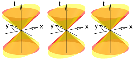
Figure 1: Light-cone structure in a coordinate system where $\vec{k}=(1,0,0)$ and $\vec{x}=(x,y,0)$ for the functions (56), (57) and (58), respectively. For this case, we can see the extreme deformation of light-cone in comparison to usual one.

The Fig. 1 represents the light-cone structures in a coordinate system where we have fixed the LV vector $\vec{\kappa}$ along the $x$-axis, $\vec{\kappa}=(1,0,0)$ and $\vec{x}=(x,y,0)$. We can see the extreme deformation of light cone in comparison to usual one. On the other hand, for the cases $\vec{x}=(x,0,z)$ and $\vec{x}=(0,y,z)$ the light-cone is only slightly different to the usual.

For microcausality analysis, we need that the functions $\Delta_{(\lambda)}(x)$ vanish for space-like vectors $x^{2}<0$. To show it, we will use the Lorentz-invariant frame where $x^{\mu}=\left(0,\vec{x}\right)$. First considering the LV Paul-Jordan function (56), we note the argument verifies the causality condition,

$$-\left|\vec{x}\right|^{2}\left(1-\left|\vec{\kappa}\right|^{2}\cos^{2}\theta\right)\,<0,$$ (59)

whenever $\left|\vec{\kappa}\right|<1$. The argument of the modified Pauli-Jordan function (57) also verifies the causality condition in the Lorentz-invariant frame,

$$-\left|\vec{x}\right|^{2}<0.$$ (60)

The argument of the third LV Pauli-Jordan function (58) becomes

$$-\left|\vec{x}\right|^{2}\left(1+\left|\vec{\kappa}\right|^{2}\sin^{2}\theta\right)<0,$$ (61)

for all values of $\left|\vec{\kappa}\right|$. Hence, we verify the functions $\Delta_{(\lambda)}(x)$ preserve the light-cone structure whenever $\left|\vec{\kappa}\right|$ is sufficiently small. Consequently, the functions $\Delta_{\left(\lambda\right)}(x)$ vanishes for spacelike vectors, assuring the microcausality. We thus conclude that the microcausality is preserved in this CPT-even and parity-odd LV electrodynamics whenever $\left|\vec{\kappa}\right|$ is sufficiently small. This microcausality analysis is in total accordance with the one performed in Ref. Schreck for this same model.

The Feynman propagator can be also computed

$${\left\langle 0\right|}TA^{\mu}(x)A^{\nu}\left(y\right){\left|0\right\rangle}=i\int\frac{d^{4}p}{\left(2\pi\right)^{4}}~{}\tilde{D}^{\mu\nu}(p)e^{-ip\cdot(x-y)},$$ (62)

where $\tilde{D}^{\mu\nu}(p)$ is given by

$$\tilde{D}^{\mu\beta}(p)=-\sum_{\lambda=0}^{3}\frac{g_{\lambda\lambda}\varepsilon_{\left(\lambda\right)}^{\mu}\left(\vec{p}\right)\varepsilon_{\left(\lambda\right)}^{\nu}\left(\vec{p}\right)\left(\delta_{\nu}^{\beta}+\delta_{0}^{\beta}\kappa_{0\nu}\right)}{\alpha_{\left(\lambda\right)}+i\varepsilon},$$ (63)

with $\alpha_{(\lambda)}$ defined in Eq. (28). The tensor $\tilde{D}^{\mu\nu}(p)$ satisfies the following equation,

$$O^{\mu}{}_{\alpha}(p)\tilde{D}^{\alpha\nu}(p)=-g^{\mu\nu}.$$ (64)

Despite the propagator (63) presents a slightly different tensor structure, the physical poles are the same found in Ref. propag .

III Failure of the gauge condition $G(A_{\mu})=\partial_{\mu}A^{\mu}+\kappa_{\mu\nu}\partial^{\mu}A^{\nu}$ in the CPT-even and parity-odd case

In this section, we show the incompatibility of the gauge fixing condition, $G(A_{\mu})=\partial_{\mu}A^{\mu}+\kappa_{\mu\nu}\partial^{\mu}A^{\nu},$ with the implementation of the Gupta-Bleuler quantization for the parity-odd and CPT-even electrodynamics. For it, we consider, without loss of generality, the case when the 3D vectors $p_{i}$ and $\kappa_{i}$ are parallel and along the positive $z$-axis. In this gauge, the expression for the operator $O^{\mu\nu}$ defining the equation of motion of the gauge field, $O^{\mu\nu}(p)A_{\nu}(p)=0$, in the momentum space, reads

$$O^{\mu\nu}(p)=\left(\begin{array}[]{cccc}{\left|{\vec{\kappa}}\right|{{}^{2}}{{\left|{\vec{p}}\right|}^{2}}-2{p_{0}}\left|{\vec{\kappa}}\right|\left|{\vec{p}}\right|+{p^{2}}}&0&0&{\left|{\vec{\kappa}}\right|\left({-{p_{0}}\left|{\vec{\kappa}}\right|\left|{\vec{p}}\right|+{p^{2}}}\right)}\\ 0&{-{p^{2}}+2{p_{0}}\left|{\vec{\kappa}}\right|\left|{\vec{p}}\right|}&0&0\\ 0&0&{-{p^{2}}+2{p_{0}}\left|{\vec{\kappa}}\right|\left|{\vec{p}}\right|}&0\\ {\left|{\vec{\kappa}}\right|\left({-{p_{0}}\left|{\vec{\kappa}}\right|\left|{\vec{p}}\right|+{p^{2}}}\right)}&0&0&{\left|{\vec{\kappa}}\right|{{}^{2}p_{0}}^{2}+2{p_{0}}\left|{\vec{\kappa}}\right|\left|{\vec{p}}\right|-{p^{2}}}\end{array}\right).$$ (65)

. The determinant provides one dispersion relation

$$\otimes(p)=p^{2}-2p_{0}|\vec{\kappa}||\vec{p}|=0,$$ (66)

with multiplicity 4. The dimension of the null space of the matrix (65) when this dispersion relation is satisfied is 3,

$$\dim\mathrm{Null}\left(O\big{|}_{\otimes(p)=0}\right)=3.$$ (67)

It implies that we only can obtain three linearly independent (l.i.) vectors which in principle would be the polarization vectors of the gauge field. As one needs four polarization vectors to realize the Gupta-Bleuler quantization, we conclude that the gauge condition, $G(A_{\mu})=\partial_{\mu}A^{\mu}+\kappa_{\mu\nu}\partial^{\mu}A^{\nu}$, does not work well in this case. A quick check of the failure of the Lorentz gauge, $G(A_{\mu})=\partial_{\mu}A^{\mu}$, can be made in the case when the vectors $\vec{p}$ and $\vec{\kappa}$ are perpendicular.

On the other hand, we can show that the condition $G(A_{\mu})=(\partial_{0}+\kappa^{0j}\partial_{j})(A_{0}+\kappa^{0k}A_{k})+\partial_{i}A^{i}$ is a suitable choice for the parity-odd and CPT-even electrodynamics. The momentum representation of the operator defining the equation of motion of the gauge field now reads

$$O^{\mu\nu}(p)=\left(\begin{array}[]{cccc}{\left|{\vec{\kappa}}\right|{{}^{2}}{{\left|{\vec{p}}\right|}^{2}}-2{p_{0}}\left|{\vec{\kappa}}\right|\left|{\vec{p}}\right|+{p^{2}}}&0&0&{\left|{\vec{\kappa}}\right|\left({{{\left|{\vec{\kappa}}\right|}^{2}}{{\left|{\vec{p}}\right|}^{2}}-2{p_{0}}\left|{\vec{\kappa}}\right|\left|{\vec{p}}\right|+{p^{2}}}\right)}\\ 0&{-{p^{2}}+2{p_{0}}\left|{\vec{\kappa}}\right|\left|{\vec{p}}\right|}&0&0\\ 0&0&{-{p^{2}}+2{p_{0}}\left|{\vec{\kappa}}\right|\left|{\vec{p}}\right|}&0\\ 0&0&0&{2{p_{0}}\left|{\vec{\kappa}}\right|\left|{\vec{p}}\right|-{{\left|{\vec{\kappa}}\right|}^{2}}{{\left|{\vec{p}}\right|}^{2}}-{p^{2}}}\end{array}\right).$$ (68)

where we have also considered the vectors $p_{i}$ and $\kappa_{i}$ to be parallel and along the positive $z$-axis. The determinant provides two dispersion relations

$$\otimes(p) = p^{2}-2p_{0}|\vec{\kappa}||\vec{p}|=0,$$ (69)

$$\boxdot(p) = p^{2}-2p_{0}|\vec{\kappa}||\vec{p}|+|\vec{\kappa}|^{2}|\vec{p}|^{2}=0,$$ (70)

both having multiplicity 2. The dimension of the null spaces of the operator (68), for each dispersion relation, is

$$\dim\mathrm{Null}\left(O^{\mu\nu}\big{|}_{\otimes=0}\right) = 2,$$ (71)

$$\dim\mathrm{Null}\left(O^{\mu\nu}\big{|}_{\boxdot=0}\right) = 2,$$ (72)

respectively. So, every null space provides two l.i. vectors totalizing four polarization vectors. Consequently, the gauge fixing condition (5) is a proper one to allow the implementation of the GB quantization in this electrodynamics.

IV Remarks and conclusion

We have studied the quantization of a CPT-even and parity-odd LV massless electrodynamics, performing the Gupta-Bleuler quantization, such as it happens in the Maxwell electrodynamics under the Feynman gauge. We have shown that the method can be implemented by using a gauge condition depending explicitly on the LV coefficients, $G(A_{\mu})=(\partial_{0}-\kappa_{j}\partial_{j})(A_{0}-\kappa_{k}A_{k})-\partial_{i}A_{i}$, which appears as a LV modified version of the Lorenz gauge. Such a choice is different from the one imposed to implement the GB quantization in the CPT-even and parity-even LV electrodynamics, $G(A_{\mu})=\partial_{\mu}A^{\mu}+\kappa_{\mu\nu}\partial^{\mu}A^{\nu}$ (see Ref. GUPTAEVEN ). We also found the set of four l.i. polarization vectors that provided the sucessful implemention of the quantization.  In Sec. III, we explicitly argue that if we use the parity-even gauge condition for the parity-odd case, we can not establish a set of linearly independent polarization vectors for arbitrary $\kappa_{i}$ and $p_{i}$. In other words, the parity-even gauge condition fails in defining a set of polarization vectors when $\kappa_{i}$ and $p_{i}$ are collinear. This problem is solved by the parity-odd gauge condition here imposed.

References

• (1) R. Casana, M. M. Ferreira Jr., and F. E. P. dos Santos, Phys. Rev. D 90, 105025 (2014).
• (2) D. Colladay, V. A. Kostelecky, Phys. Rev. D 55, 6760 (1997); D. Colladay, V. A. Kostelecky Phys. Rev. D 58, 116002 (1998); S. R. Coleman and S. L. Glashow, Phys. Rev. D 59, 116008 (1999).
• (3) S.M. Carroll, G.B. Field and R. Jackiw, Phys. Rev. D 41, 1231 (1990).
• (4) V. A. Kostelecky and M. Mewes, Phys. Rev. Lett. 87, 251304 (2001); V. A. Kostelecky and M. Mewes, Phys. Rev. D 66, 056005 (2002); V. A. Kostelecky and M. Mewes, Phys. Rev. D 80, 015020 (2009); V. A. Kostelecky and M. Mewes, Phys. Rev. Lett. 97, 140401 (2006).
• (5) A.A. Andrianov and R. Soldati, Phys. Rev. D 51, 5961 (1995); Phys. Lett. B 435, 449 (1998); A.A. Andrianov, R. Soldati and L. Sorbo, Phys. Rev. D 59, 025002 (1998); A. A. Andrianov, D. Espriu, P. Giacconi, R. Soldati, J. High Energy Phys. 0909, 057 (2009); J. Alfaro, A.A. Andrianov, M. Cambiaso, P. Giacconi, R. Soldati, Int. J. Mod.Phys. A 25, 3271 (2010); V. Ch. Zhukovsky, A. E. Lobanov, E. M. Murchikova, Phys. Rev. D73 065016, (2006); W. F. Chen and G. Kunstatter, Phys. Rev. D 62, 105029 (2000).
• (6) C. Adam and F. R. Klinkhamer, Nucl. Phys. B 607, 247 (2001); C. Adam and F. R. Klinkhamer, Nucl. Phys. B 657, 214 (2003).
• (7) A. P. Baeta Scarpelli, H. Belich, J. L. Boldo, J. A. Helayel-Neto, Phys. Rev. D 67, 085021 (2003).
• (8) R. Casana, M. M. Ferreira Jr, A. R. Gomes, F. E. P. dos Santos, Phys. Rev. D 82, 125006 (2010).
• (9) M. Cambiaso, R. Lehnert, R. Potting, Phys. Rev. D 85, 085023 (2012).
• (10) M. Schreck, Phys. Rev. D 86, 065038 (2012).
• (11) M. Schreck, Phys. Rev. D 89, 085013 (2014).
• (12) M. A. Hohensee, D. F. Phillips, R. L. Walsworth, Covariant quantization of Lorentz-violating electromagnetism, arXiv:1210.2683.
• (13) D. Colladay, P. McDonald, and R. Potting, Phys. Rev. D 89, 085014 (2014)
• (14) D. Colladay, Covariant photon quantization in the SME, arXiv:1309.5890.
• (15) D. Colladay and P. McDonald, Phys. Rev. D 93, 125007 (2016).
• (16) D. Colladay, P. McDonald, J. P. Noordmans, and R. Potting , Covariant Quantization of CPT-violating Photons, arXiv:1610.00169.
• (17) V. A. Kostelecky, N. Russell, Rev. Mod. Phys. 83, 11 (2011).
• (18) B. Altschul, Phys. Rev. Lett. 98, 041603 (2007).
• (19) S. N. Gupta, Proc. Phys. Soc. A 63, 681 (1950).
• (20) K. Bleuler, Helv. Phys. Acta 23, 567 (1950).
• (21) N. Nakanishi, Prog. Theo. Phys. 38, 881 (1967).