Abstract: Multi-valued partial CFL functions are functions computed along accepting computation paths by one-way nondeterministic pushdown automata, equipped with write-only output tapes, which are allowed to reject an input, in comparison with single-valued partial CFL functions. We give an answer to a fundamental question, raised by Konstantinidis, Santean, and Yu [Act. Inform. 43 (2007) 395–417], of whether all such multi-valued partial CFL functions can be refined by single-valued partial CFL functions. We negatively solve this open question by presenting a special multi-valued partial CFL function as an example function and by proving that no refinement of this particular function becomes a single-valued partial CFL function. This contrasts an early result of Kobayashi [Inform. Control 15 (1969) 95–109] that multi-valued partial NFA functions are always refined by single-valued NFA functions, where NFA functions are computed by one-way nondeterministic finite automata with output tapes. Our example function turns out to be unambiguously 2-valued, and thus we obtain a stronger separation result, in which no refinement of unambiguously 2-valued partial CFL functions can be single-valued. For the proof of this fact, we first introduce a new concept of colored automata having no output tapes but having “colors,” which can simulate pushdown automata equipped with constant-space output tapes. We then conduct an extensive combinatorial analysis on the behaviors of transition records of stack contents (called stack histories) of these colored automata.

Keywords: multi-valued partial function, CFL function, NFA function, refinement, pushdown automaton, context-free language, colored automaton, stack history

1 Resolving a Fundamental Question

Since early days of automata and formal language theory, multi-valued partial functions, computed by various types of automata equipped with supplemental write-only output tapes, have been investigated extensively. To keep a restricted nature of memory usage, we require the automata to write output symbols in an oblivious way; namely, the automata move their output-tape heads to new blank cells whenever they write non-blank output symbols. We succinctly refer such output tapes to “write only.” Among those types of functions, we intend to spotlight CFL functions (also known as algebraic transductions), which are computed by one-way nondeterministic pushdown automata (succinctly abbreviated as npda’s) whose input-tape heads move only in one direction (from the left to the right) with write-only output tapes. Such functions were formally discussed in 1963 by Evey [2] and Fisher [4]. The acronym CFL stands for context-free languages because, with no output tapes, the machines recognize precisely context-free languages. Therefore, those functions naturally inherit certain distinctive traits from the context-free languages; however, their behaviors are in essence quite different from the behaviors of the languages. Such intriguing properties of those functions have been addressed occasionally in the past literature (e.g.,  [1, 2, 4, 7, 12, 14]).

Along their numerous accepting computation paths, npda’s can produce various output values on their output tapes. We flexibly allow npda’s to reject an input, producing no valid output values. When the number of output values is always limited to at most one, we obtain single-valued partial functions. Such single-valued partial functions can be obviously treated as multi-valued partial functions, but multi-valued partial functions are, in general, not single-valued. For expressing a relationship between multi-valued and single-valued partial functions, it is therefore more appropriate to ask a question of whether multi-valued partial functions can be refined by single-valued partial functions, where “refinement” is a notion discussed initially for NP functions [8] and it refers to a certain natural restriction on the outcomes of multi-valued functions. To be more precise, we say that a function $g$ is a refinement (also called “uniformization” [7]) of another function $f$ if and only if (i) $f$ and $g$ have the same domain and (ii) for every input $x$ in the domain of $f$, all output values of $g$ on $x$ are also output values of $f$ on the same input $x$. When $g$ is particularly single-valued, $g$ acts as a “selection” function that picks exactly one value out of a set of output values of $f$ on $x$ whenever the set is nonempty. This refinement notion is known to play a significant role also in language recognition. In a polynomial-time setting, for instance, if we can effectively find an accepting computation path of any polynomial-time nondeterministic Turing machine, then every multi-valued partial NP function (which is computed by a certain polynomial-time nondeterministic Turing machine) has a refinement in the form of single-valued NP function. Therefore, this “no-refinement” claim for multi-valued partial NP functions immediately leads to a negative answer to the long-standing $\mathrm{P}=?\mathrm{NP}$ question. More generally, multi-valued partial $\Sigma^{\mathrm{P}}_{k}$-functions in the so-called NPMV-hierarchy $\{\Sigma^{\mathrm{P}}_{k}\mathrm{MV},\Pi^{\mathrm{P}}_{k}\mathrm{MV}\mid k\geq 1\}$ are not in general refined by single-valued partial $\Sigma^{\mathrm{P}}_{k}$-functions as long as the polynomial(-time) hierarchy forms an infinite hierarchy [3, 9].

Returning to automata theory, we can discuss a similar refinement question on CFL functions in hope that we resolve it without any unproven assumption, such as the separation of the polynomial hierarchy. Along this line of research, the first important step was taken by Kobayashi [6] in 1969. He gave an affirmative answer to the refinement question on multi-valued partial NFA functions, which are computed by one-way nondeterministic finite automata (or nfa’s, in short) with write-only output tapes; namely, multi-valued partial NFA functions can be refined by appropriate single-valued partial NFA functions. Konstantinidis, Santean, and Yu [7] discussed a similar question concerning multi-valued partial CFL functions. They managed to obtain a partial affirmative answer but unfortunately they left the whole question open.

This paper is focused on CFL functions whose output values are produced by npda’s that halt in linear time (that is, all computation paths terminate in time $O(n)$, where $n$ is the size of input) with write-only output tapes. By adopting succinct notations from [12, 14], we express as $\mathrm{CFLMV}$ the collection of all such CFL functions and we also write $\mathrm{CFLSV}$ for a collection of all single-valued partial functions in $\mathrm{CFLMV}$. As a concrete example of our CFL function, let us consider $f$ defined by setting $f(1^{n}\#x)$ to be the set of all substrings of $x$ of length between $1$ and $n$, exactly when $1\leq n\leq|x|$. This function $f$ is a multi-valued partial CFL function and the following function $g$ is an obvious refinement of $f$; the set $g(1^{n}\#x)$ is composed only of the first symbol of $x$ whenever $1\leq n\leq|x|$. Notice that $g$ belongs to $\mathrm{CFLSV}$.

For a further discussion, it is beneficial to introduce another succinct notation concerning “refinement.” Given two classes ${\cal F}$ and ${\cal G}$ of multi-valued partial functions, we write ${\cal F}\sqsubseteq_{ref}{\cal G}$ if every function in ${\cal F}$ can be refined by an appropriately chosen function in ${\cal G}$. Using this notation, the aforementioned refinement question of Konstantinidis et al. regarding CFL functions can be rephrased neatly as follows.

Question 1.1

Is it true that $\mathrm{CFLMV}\sqsubseteq_{ref}\mathrm{CFLSV}$?

Various extensions of $\mathrm{CFLMV}$ in Question 1.1 are also possible. We state one such possible extension. Yamakami [14] lately introduced a functional hierarchy $\{\Sigma^{\mathrm{CFL}}_{k}\mathrm{MV},\Pi^{\mathrm{CFL}}_{k}\mathrm{MV}\mid k\geq 1\}$ (called the CFLMV hierarchy), which is built upon multi-valued partial CFL functions by applying Turing relativization and a complementation operation (see Section 4), analogously to the aforementioned NPMV hierarchy $\{\Sigma^{\mathrm{P}}_{k}\mathrm{MV},\Pi^{\mathrm{P}}_{k}\mathrm{MV}\mid k\geq 1\}$ over multi-valued partial NP functions [3, 9]. Its single-valued version is customarily denoted by $\{\Sigma^{\mathrm{CFL}}_{k}\mathrm{SV},\Pi^{\mathrm{CFL}}_{k}\mathrm{SV}\mid k\geq 1\}$. The function $g$ defined as $g(w)=\{x\in\{0,1\}^{*}\mid\exists\,u,v\,[w=uxxv]\}$ for each $w\in\{0,1\}^{*}$ is a simple example of function in $\Sigma^{\mathrm{CFL}}_{2}\mathrm{MV}$.

Our focal question, Question 1.1, can be further generalized to the following.

Question 1.2

Does $\Sigma^{\mathrm{CFL}}_{k}\mathrm{MV}\sqsubseteq_{ref}\Sigma^{\mathrm{CFL}}_{k}\mathrm{SV}$ hold for each index $k\geq 1$?

When $k\geq 3$, Yamakami [14] shed partial light on this general question. He was able to show that, for every index $k\geq 3$, $\Sigma^{\mathrm{CFL}}_{k-1}=\Sigma^{\mathrm{CFL}}_{k}$ implies $\Sigma^{\mathrm{CFL}}_{k}\mathrm{MV}\sqsubseteq_{ref}\Sigma^{\mathrm{CFL}}_{k}\mathrm{SV}$, where $\Sigma^{\mathrm{CFL}}_{k}$ is the $k$th level of the CFL hierarchy [13], which is the language counterpart of the CFLMV hierarchy. Since the collapse of the CFL hierarchy is closely related to that of the polynomial hierarchy, the answer to Question 1.2 (when $k\geq 3$) might possibly be quite difficult to obtain. See Section 4 for a further discussion. Nevertheless, the remaining cases of $k=1,2$ have been left unsolved.

In this paper, without relying on any unproven assumption, we solve Question 1.2 negatively when $k=1$; therefore, our result completely settles Question 1.1. Our solution actually gives an essentially stronger statement than what we have discussed so far. To explain this statement, we need a new function class $\mathrm{CFL2V}$ as the collection of all functions $f$ in $\mathrm{CFLMV}$ satisfying the condition that the number of output values of $f$ on each input should be at most $2$. We actually obtain the following statement.

Theorem 1.3

$\mathrm{CFL2V}\not\sqsubseteq_{ref}\mathrm{CFLSV}$.

Since $\mathrm{CFLSV}\subseteq\mathrm{CFL2V}\subseteq\mathrm{CFLMV}$ holds, Theorem 1.3 clearly leads to a negative answer to Question 1.1. The proof of this theorem is essentially a manifestation of the following intuition: since an npda relies on limited functionality of its memory device (a stack), along any single computation path, it cannot simulate simultaneously two independent computation paths of another npda.

Instead of providing a detailed proof for Theorem 1.3, we wish to present a simple and clear argument to demonstrate a slightly stronger result regarding a subclass of $\mathrm{CFL2V}$. To justify an introduction of such a subclass, we need to address that even if a function $f$ is single-valued, its underlying npda on each input may have numerous accepting computation paths, each of which produces the same value of $f$. Hence, controlling the number of those accepting computation paths may be difficult for npda’s. We thus restrict our attention on special npda’s that have “few” accepting computation paths for each output value. Let us first call an npda $N$ with a write-only output tape unambiguous if, for every input $x$ and any output value $y$, $N$ has exactly one accepting computation path producing $y$. Finally, we denote by $\mathrm{UCFL2V}$ the class of all $2$-valued partial functions computed in linear time by unambiguous npda’s equipped with output tapes. Succinctly, those functions are called unambiguously 2-valued. Obviously, $\mathrm{UCFL2V}\subseteq\mathrm{CFL2V}$ holds.

Throughout this paper, we wish to show the following stronger separation result (than Theorem 1.3), which is referred to as the “main theorem” in the subsequent sections.

Theorem 1.4 (Main Theorem)

$\mathrm{UCFL2V}\not\sqsubseteq_{ref}\mathrm{CFLSV}$.

Following a brief explanation of key notions and notation in Section 2, we will give in Section 3 the proof of Theorem 1.4, completing the proof of Theorem 1.3 as well. Our proof will start in Sections 3.1 with a presentation of our example function $h_{3}$, a member of $\mathrm{UCFL2V}$. The proof will then proceed, by way of contradiction, starting with a faulty assumption that a certain refinement, say, $g$ of $h_{3}$ exists in $\mathrm{CFLSV}$. Thus, there is an npda computing $g$ using a write-only output tape. For our proof, however, we wish to avoid the messy handling of the output tape of this npda and seek a simpler model of automaton for an easier analysis of its behaviors. For this purpose, we will introduce in Section 3.2 a new concept of “colored” automaton—a new type of automaton having no output tape but having “colors”—which can simulate any npda equipped with an output tape that computes $g$. To each accepting computation path of such colored automata, we assign a certain color if the machine pushes the same colored symbols into a stack along this computation path.

To lead to the desired contradiction, we are focused on accepting colored computation paths of a colored automaton and see how the computation paths can turn into different colors if we alter certain portions of input strings. The proof will further exploit special properties of such a colored automaton by analyzing the behaviors of its time transition record of stack contents (called a stack history) generated by this colored automaton. The detailed combinatorial analysis of the stack history will be presented in Sections 3.3–3.6. The analysis itself is interesting on its own right. The proof of the main theorem will be split into two cases. In Case 1, the proof is supported by two key statements, Proposition 3.7 and Proposition 3.16 (for a special case, Proposition 3.13), in which we estimate the height of stack contents at certain points of a stack history. The proofs of these propositions are quite contrive to some extent. These estimations provide two contradictory upper and lower bounds of the height, leading to the desired contradiction. In Case 2, we transform this case back to Case 1 by constructing a “reversed” colored automaton in Proposition 3.18 in Section 3.6.

We expect that colored automata may find useful applications to other issues arising in automata theory and we strongly hope that our analysis of stack history may shed another insight into the behaviors of other intriguing automata models.

2 Preparation for the Proof

Before giving the awaiting proof of the main theorem (Theorem 1.4) in Section 3, we wish to explain key notions and notation necessary to read through the rest of this paper.

Let $\mathbb{N}$ denote the set of all natural numbers (i.e., nonnegative integers) and define $\mathbb{N}^{+}=\mathbb{N}-\{0\}$. Given two integers $m$ and $n$ with $m\leq n$, the notation $[m,n]_{\mathbb{Z}}$ denotes the integer interval $\{m,m+1,m+2,\ldots,n\}$. When $n\geq 1$, we further abbreviate $[1,n]_{\mathbb{Z}}$ as $[n]$. All logarithms are taken to the base $2$ unless otherwise stated. Given a finite set $A$, ${\cal P}(A)$ denotes the power set of $A$ (i.e., the collection of all subsets of $A$). The notation $|A|$ for a finite set $A$ refers to its cardinality (i.e., the number of all distinct elements in $A$).

An alphabet is a finite nonempty set of “symbols” or “letters.” Given such an alphabet $\Sigma$, a string $x$ over $\Sigma$ is a finite series of symbols taken from $\Sigma$ and the length (or size) of $x$, denoted by $|x|$, is the total number of symbols in $x$. We use $\lambda$ to express the empty string of length $0$. The set of all strings over $\Sigma$ is denoted by $\Sigma^{*}$ and a language over $\Sigma$ is a subset of $\Sigma^{*}$. Let $\Sigma^{+}=\Sigma^{*}-\{\lambda\}$. The set $\Sigma^{n}$ for a number $n\in\mathbb{N}$ is composed of all strings of length $n$ and the set $\Sigma^{\geq k}$ (resp., $\Sigma^{\leq k}$) consists of all strings of length at least $k$ (resp., at most $k$). For a symbol $a$ and a language $A$, the notation $aA$ stands for the set $\{ax\mid x\in A\}$. Given two strings $x$ and $y$ over the same alphabet, the notation $x\sqsubseteq y$ indicates that $x$ is a substring of $y$; namely, $y$ equals $uxv$ for certain two strings $u$ and $v$. Moreover, for a string $x$ and an index $i\in[|x|]$, $(x)_{i}$ expresses a unique substring made up only of the first $i$ symbols of $x$. Such a string is also called a prefix. For example, $(0100)_{1}=0$ and $(0100)_{3}=010$. Clearly, $(x)_{i}\sqsubseteq x$ and $(x)_{|x|}=x$ hold. Given a string $x=x_{1}x_{2}\cdots x_{n-1}x_{n}$ with $x_{i}\in\Sigma$ for all $i\in[n]$, the reversal of $x$, denoted by $x^{R}$, is the string $x_{n}x_{n-1}\cdots x_{2}x_{1}$.

A multi-valued partial function generally maps elements of a given set to subsets of another (possibly the same) set. Slightly different from a conventional notation (e.g.,  [8, 9]), we write $f:A\rightarrow{\cal P}(B)$ for two sets $A$ and $B$ to refer to a multi-valued partial function that takes an element in $A$ as input and produces a certain number of elements in $B$. In particular, when $f(x)=\emptyset$, we conventionally say that $f(x)$ is undefined. The domain of $f$, denoted by $\mbox{dom}(f)$, is therefore the set $\{x\in A\mid f(x)\text{ is not undefined }\}$. Given a constant $k\in\mathbb{N}^{+}$, $f$ is said to be $k$-valued if $|f(x)|\leq k$ holds for every input $x$ in $A$. For two multi-valued partial functions $f,g:A\rightarrow{\cal P}(B)$, we say that $g$ is a refinement of $f$ (or $f$ is refined by $g$), denoted by $f\sqsubseteq_{ref}g$, if (i) $\mbox{dom}(f)=\mbox{dom}(g)$ and (ii) $g(x)\subseteq f(x)$ (set inclusion) holds for every $x\in\mbox{dom}(g)$ [8]. For any two function classes ${\cal F}$ and ${\cal G}$, the succinct notation ${\cal F}\sqsubseteq_{ref}{\cal G}$ is used when every function in ${\cal F}$ has a refinement in ${\cal G}$.

Our mechanical model of computation is a one-way nondeterministic pushdown automaton (or an npda, for short) with/without a write-only output tape, allowing $\lambda$-moves (or $\lambda$-transitions). We use an infinite input tape, which holds two special endmarkers: the left endmarker $|\!\!\mathrm{c}$ and the right endmarker $\$$. Let $\check{\Sigma}$ stand for the set $\Sigma\cup\{|\!\!\mathrm{c},\$\}$. In addition, we use a semi-infinite output tape, on which its tape head is initially positioned at the first (i.e.,  the leftmost) tape cell and moves only in one direction (to the right) whenever it writes a non-blank symbol. Formally, an npda $M$ with an output tape is a tuple $(Q,\Sigma,\{|\!\!\mathrm{c},\$\},\Gamma,\Theta,\delta,q_{0},\bot,Q_{acc},Q_{rej})$ with a finite set $Q$ of inner states, an input alphabet $\Sigma$, a stack alphabet $\Gamma$, an output alphabet $\Theta$, the initial state $q_{0}\in Q$, the bottom marker $\bot\in\Gamma$, a set $Q_{acc}$ (resp., $Q_{rej}$) of accepting (resp., rejecting) states satisfying $Q_{acc}\cup Q_{rej}\subseteq Q$, and a transition function $\delta:(Q-Q_{halt})\times(\check{\Sigma}\cup\{\lambda\})\times\Gamma\rightarrow{\cal P}(Q\times\Gamma^{*}\times(\Theta\cup\{\lambda\}))$, where $Q_{halt}=Q_{acc}\cup Q_{rej}$. The input tape is indexed by natural numbers with $|\!\!\mathrm{c}$ in the $0$th cell. When an input $x=x_{1}x_{2}\cdots x_{n}$ of length $n$ is given, it is placed in cells indexed from $1$ to $n$, where $\$$ is at the $(n+1)$th cell. A stack holds a series $s_{k}s_{k-1}\cdots s_{1}s_{0}$ of stack symbols in such a way that $s_{0}=\bot$ and $s_{k}$ is the topmost symbol. We demand that $M$ should neither remove $\bot$ nor replace it with any other symbol at any step; that is, for any tuple $(p,q,s,\sigma,\tau)$, $(p,s,\tau)\notin\delta(q,\sigma,\bot)$ holds if $s$ does not contain $\bot$ at its bottom. Conventionally, we say that the stack is empty if it contains only the bottom marker $\bot$. Moreover, $M$ is not allowed to use $\bot$ as an ordinary stack symbol; that is, $(p,s,\tau)\notin\delta(q,\sigma,\gamma)$ if $\gamma\neq\bot$ and $\tau$ contains $\bot$. The output tape must be write-only; namely, whenever $M$ writes a non-blank symbol on this tape, its tape head must move to the right. It is important to recognize two types of $\lambda$-moves. When $\delta$ is applied to tuple $(q,\lambda,\gamma)$, $M$ modifies the current contents of its stack and its output tape while neither scanning input symbols nor moving its input-tape head. In contrast, when $(p,w,\lambda)\in\delta(q,\sigma,\gamma)$ holds, $M$ neither moves its output-tape head nor writes any non-blank symbol onto the output tape.

A configuration of $M$ on input $x$ is a triplet $(q,i,w)$, in which $M$ is in inner state $q$ (with $q\in Q$), its tape head scans the $i$th cell (with $i\in[0,|x|+1]_{\mathbb{Z}}$), and its stack contains $w$ (with $w\in\Gamma^{*}$). The initial configuration is $(q_{0},0,\bot)$ and an accepting (resp., a rejecting) configuration is a configuration with an accepting state (resp., a rejecting state). A halting configuration is either an accepting or a rejecting configuration. A computation path of $M$ on $x$ is a series of configurations of $M$ on $x$, starting with the initial configuration, for which any non-initial configuration in the series must be reached from its predecessor by a single application of $\delta$.

Whenever we need to discuss an npda having no output tape, we drop “$\Theta$” as well as “$\Theta\cup\{\lambda\}$” from the aforementioned definition of $M$ and $\delta$. As stated in Section 1, we consider only npda’s whose computation paths all terminate within $O(n)$ steps, where $n$ refers to any input size, and this particular condition concerning the termination of computation is conventionally called the termination condition [13]. Throughout this paper, all npda’s are implicitly assumed to satisfy this termination condition.

In general, an output (outcome or output string) of $M$ along a given computation path refers to a string over $\Theta$ written down on the output tape when the computation path terminates. Such an output is called valid (or legitimate) if the corresponding computation path is an accepting computation path (i.e.,  $M$ enters an accepting state along this computation path). Given a function $f$, we say that an npda $M$ with an output tape computes $f$ if, on every input $x$, $M$ produces exactly all the strings in $f(x)$ as valid outputs; namely, for every pair $(x,y)$, $y\in f(x)$ if and only if $y$ is a valid outcome of $M$ on the input $x$. Notice that an npda can generally produce more than one valid output string, its computed function inherently becomes multi-valued. Because invalid outputs produced by $M$ are all discarded from our arguments in the subsequent sections, we will refer to valid outputs as just “outputs” unless otherwise stated.

The notation $\mathrm{CFLMV}$ (resp., $\mathrm{CFL}{k}\mathrm{V}$ for a fixed constant $k\in\mathbb{N}^{+}$) stands for the class of all multi-valued (resp., $k$-valued) partial functions that can be computed by appropriate npda’s with write-only output tapes in linear time. When $k=1$, in particular, we customarily write $\mathrm{CFLSV}$ instead of $\mathrm{CFL}{1}\mathrm{V}$. In addition, we define $\mathrm{UCFL}{k}\mathrm{V}$ as the collection of all functions $f$ in $\mathrm{CFL}{k}\mathrm{V}$ for which an appropriate npda $M$ equipped with an output tape computes $f$ with the extra condition (called the unambiguous computation condition) that, for every input $x$ and every value $y$ in $f(x)$, there exists exactly one accepting computation path of $M$ on $x$ producing $y$. It follows by their definitions that $\mathrm{UCFL}{k}\mathrm{V}\subseteq\mathrm{CFL}{k}\mathrm{V}\subseteq\mathrm{CFLMV}$. Since any function producing exactly $k+1$ values cannot belong to $\mathrm{CFL}{k}\mathrm{V}$ by definition, $\mathrm{CFL}{k}\mathrm{V}\neq\mathrm{CFL}{(k+1)}\mathrm{V}$ holds; therefore, in particular, we obtain $\mathrm{CFLSV}\neq\mathrm{CFLMV}$. Notice that this inequality does not directly lead to the desired conclusion $\mathrm{CFLMV}\not\sqsubseteq_{ref}\mathrm{CFLSV}$.

To describe behaviors of an npda’s stack, we closely follow terminology from [11, 15]. A stack content is formally a series $z_{m}z_{m-1}\cdots z_{1}z_{0}$ of stack symbols sequentially stored into a stack (in our convention, $z_{0}$ is the bottom marker $\bot$ and $z_{m}$ is a symbol at the top of the stack). A stack content at the $i$th cell position refers to a stack content obtained just after the tape head scans and then moves off the $i$th cell of the input tape. A series of stack contents produced along a computation path is briefly referred to as a stack history.

3 Proof of the Main Theorem

Our ultimate goal is to solve negatively a question that was posed in [7] and reformulated in [14] as in the form of Question 1.1. For this purpose, we intend to prove the main theorem (Theorem 1.4). As an example of a non-refinable function that witnesses the theorem, we will present a special function, called $h_{3}$, which belongs to $\mathrm{UCFL2V}$ (shown in Section 3.1), and then give an explanation of why no refinement of this function is found in $\mathrm{CFLSV}$, resulting in the main theorem, namely, $\mathrm{UCFL2V}\not\sqsubseteq_{ref}\mathrm{CFLSV}$. To simplify our proof, we will introduce in Section 3.2 a computational model of colored automata, which have no output tapes but have “colors” to specify their outcomes. We will conduct a combinatorial analysis on a stack history of such colored automata in Section 3.3–3.6.

3.1 An Example Function

Our example function $h_{3}$ is a natural extension of a well-known deterministic context-free language $\{x\#x^{R}\mid x\in\{0,1\}^{*}\}$ (marked even-length palindromes), where $\#$ is a distinguished symbol not in $\{0,1\}$, used as a separator. Let us define two supporting languages $L=\{x_{1}\#x_{2}\#x_{3}\mid x_{1},x_{2},x_{3}\in\{0,1\}^{*}\}$ and $L_{3}=\{w\mid\exists x_{1},x_{2},x_{3}[w=x_{1}\#x_{2}\#x_{3}\in L,\exists(i,j)\in I_{3}\;[x_{i}^{R}=x_{j}]]\}$, where $I_{3}=\{(i,j)\mid i,j\in\mathbb{N}^{+},1\leq i<j\leq 3\}$. We then introduce the desired function $h_{3}$ by setting $h_{3}(w)=\{0^{i}1^{j}\mid(i,j)\in I_{3},x_{i}^{R}=x_{j}\}$ if $w=x_{1}\#x_{2}\#x_{3}\in L$, and $h_{3}(w)=\emptyset$ otherwise. It thus follows that $L_{3}=\{w\in L\mid h_{3}(w)\neq\emptyset\}$. As simple examples, if $w$ has the form $x\#x^{R}\#y$ with $x\neq y$, then $h_{3}(w)$ equals $\{011\}$; in contrast, if $w=x\#x^{R}\#x$, then $h_{3}(w)$ is $\{011,00111\}$.

Let us verify the following proposition.

Proposition 3.1

The above function $h_{3}$ is in $\mathrm{UCFL2V}$.

Proof.

Obviously, the function $h_{3}$ is 2-valued. Targeting $h_{3}$, let us consider the following npda $M$ equipped with a write-only output tape. On any input $w$, $M$ deterministically checks whether $w$ is of the form $x_{1}\#x_{2}\#x_{3}$ in $L$ by moving its input-tape head from the left to the right by counting the number of $\#$ in $w$. At the same time, $M$ guesses (i.e., nondeterministically chooses) a pair $(i,j)\in I_{3}$, writes $0^{i}1^{j}$ onto its output tape, stores $x_{i}$ into a stack, and then checks whether $x_{i}^{R}$ matches $x_{j}$ by retrieving $x_{i}$ in a reverse order from the stack. If $x_{i}^{R}=x_{j}$ holds, then $M$ enters an accepting state; otherwise, it enters a rejecting state.

To be more formal, the desired npda $M=(Q,\Sigma,\{|\!\!\mathrm{c},\$\},\Gamma,\Theta,\delta,q_{0},\bot,Q_{acc},Q_{rej})$ is defined as follows. Let $\Sigma=\{0,1,\#\}$, $\Gamma=\{0,1,\bot\}$, and $\Theta=\{0,1\}$. Moreover, let $Q_{acc}=\{q_{acc}\}$ and $Q_{rej}=\{q_{rej}\}$. The transition function $\delta$ consists of the following transitions. The first move of $M$ is a nondeterministic move of $\delta(q_{0},|\!\!\mathrm{c},\bot)=\{(q_{12}^{(0)},\bot,01^{2}),(q_{23}^{(0)},\bot,0^{2}1^{3}),(q_{13}^{(0)},\bot,01^{3})\}$. With respect to $q_{12}^{(0)}$, this first step is followed by a series of transitions: $\delta(q_{12}^{(0)},\sigma,a)=\{(q_{12}^{(0)},\sigma a,\lambda)\}$, $\delta(q_{12}^{(0)},\#,a)=\{(q_{12}^{(1)},a,\lambda)\}$, $\delta(q_{12}^{(1)},\sigma,\sigma)=\{(q_{12}^{(1)},\lambda,\lambda)\}$, $\delta(q_{12}^{(1)},\#,\bot)=\{(q_{12}^{(2)},\bot,\lambda)\}$, $\delta(q_{12}^{(2)},\sigma,\bot)=\{(q_{12}^{(2)},\bot,\lambda)\}$, and $\delta(q_{12}^{(2)},\$,\bot)=\{(q_{acc},\bot,\lambda)\}$, where $\sigma\in\Sigma$ and $a\in\Gamma$. For all other transitions, $M$ changes its inner states to $q_{rej}$. For the other two states $q_{23}^{(0)}$ and $q_{13}^{(0)}$, we can define similar sets of transitions and thus we omit their precise descriptions.

It therefore follows by the above definition that, for each choice of $(i,j)$ in $I_{3}$, there is at most one accepting computation path producing $0^{i}1^{j}$. It is not difficult to verify that $M$ correctly computes $h_{3}$. Therefore, $h_{3}$ belongs to $\mathrm{UCFL2V}$. ∎

We have obtained the example function $h_{3}$, which belongs to $\mathrm{UCFL2V}$. To complete the proof of the main theorem, it therefore suffices to verify the following proposition regarding the non-existence of a refinement of the function $h_{3}$.

Proposition 3.2

The function $h_{3}$ has no refinement in $\mathrm{CFLSV}$.

In the subsequent five subsections, we will describe the proof of Proposition 3.2 and thus derive the main theorem.

3.2 Colored Automata

Our proof of Proposition 3.2 proceeds by way of contradiction. To lead to the desired contradiction, we first assume that $h_{3}$ has a refinement, say, $g$ in $\mathrm{CFLSV}$. Since $g$ is single-valued, in what follows, we rather write $g(x)=y$ instead of $g(x)=\{y\}$ for $x\in\mbox{dom}(f)$. Take an npda $N$ computing $g$ with a write-only output tape. Assume that $N$ has the form $(Q,\Sigma,\{|\!\!\mathrm{c},\$\},\Gamma,\Theta,\delta,q_{0},\bot,Q_{acc},Q_{rej})$ with a transition function $\delta:(Q-Q_{halt})\times(\check{\Sigma}\cup\{\lambda\})\times\Gamma\rightarrow{\cal P}(Q\times\Gamma^{*}\times(\Theta\cup\{\lambda\}))$. Notice that $\Sigma=\Theta=\{0,1\}$ by the definition of $g$.

Unfortunately, we find it difficult to directly follow and analyze the moves of $N$’s output-tape head. To overcome this difficulty, we try to modify $N$ into a new variant of npda having no output tape. As seen later, this modification is possible because $g$’s output values are limited only to strings of constant lengths. Now, let us introduce this new machine, dubbed as “colored” automaton, which has no output tapes but uses “colored” stack symbols. Using a finite set $C$ of “colors,” a colored automaton $M=(Q^{\prime},\Sigma,\{|\!\!\mathrm{c},\$\},\Gamma^{\prime},C,\delta^{\prime},q^{\prime}_{0},\bot,Q^{\prime}_{acc},Q^{\prime}_{rej})$ partitions its stack alphabet $\Gamma^{\prime}$, except for the bottom marker $\bot$, into sets $\{\Gamma^{\prime}_{\xi}\}_{\xi\in C}$; namely, $\bigcup_{\xi\in C}\Gamma^{\prime}_{\xi}=\Gamma^{\prime}-\{\bot\}$ and $\Gamma^{\prime}_{\xi}\cap\Gamma^{\prime}_{\xi^{\prime}}=\emptyset$ for any distinct pair $\xi,\xi^{\prime}\in C$. Let $\tilde{\Gamma}_{\xi}=\Gamma^{\prime}_{\xi}\cup\{\bot\}$ for each color $\xi\in C$. For a color of stack symbol $\gamma$, we say that $\gamma$ is in color $\xi$ if $\gamma$ is in $\tilde{\Gamma}_{\xi}$. Note that $\bot$ has all colors.

The transition function $\delta^{\prime}$ maps $(Q^{\prime}-Q^{\prime}_{hatl})\times(\check{\Sigma}\cup\{\lambda\})\times\Gamma^{\prime}$ to ${\cal P}(Q^{\prime}\times(\Gamma^{\prime})^{*})$. Given a substring $z$ of input $x$, we say that $M$ read off $z$ if $M$ starts with reading the leftmost symbol of $z$, continues reading the entire symbols of $z$, makes all possible $\lambda$-moves after reading an input symbol, and moves its tape head out of $z$ after processing the rightmost symbol of $z$. The notions of computation, computation path, and accepting/rejecting computation path are defined similarly to the case of npda’s.

Given a color $\xi\in C$, we call a computation path of $M$ a $\xi$-computation path if all configurations along this computation path use only stack symbols in color $\xi$. In this case, such a computation path is also said to be colored (in color $\xi$). Most importantly, we demand that all computation paths of $M$ should be colored. An output of $M$ on input $x$ is composed of all colors $\xi$ in $C$ for which there is an accepting $\xi$-computation path of $M$ on $x$.

Let us verify that the aforementioned CFLSV function $g$ can be computed by an appropriately chosen colored automaton.

Lemma 3.3

Assuming $g\in\mathrm{CFLSV}$, there exists a colored automaton $M$ that computes $g$.

Proof.

Associated with the set $I_{3}$ introduced in Section 3.1, we define a new set $\bar{I}_{3}=\{0^{i}1^{j}\mid(i,j)\in I_{3}\}$ and another set $\bar{I}^{part}_{3}$ composed of all substrings of any string in $\bar{I}_{3}$. Notice that $\lambda\in\bar{I}^{part}$. Let us recall the aforementioned npda $N=(Q,\Sigma,\{|\!\!\mathrm{c},\$\},\Gamma,\Theta,\delta,q_{0},\bot,Q_{acc},Q_{rej})$ that computes $g$ with its write-only output tape. Now, we wish to construct a new colored automaton $M=(Q^{\prime},\Sigma,\{|\!\!\mathrm{c},\$\},\Gamma^{\prime},\bar{I}_{3},\delta^{\prime},q^{\prime}_{0},\bot,Q^{\prime}_{acc},Q^{\prime}_{rej})$ that simulates $N$.

We start by setting $Q^{\prime}=Q\times(\bar{I}_{3}\cup\{\lambda\})\times\bar{I}^{part}_{3}$ and $q^{\prime}_{0}=(q_{0},\lambda,\lambda)$. In addition, let $\Gamma^{\prime}=\{\bot\}\cup\{\tau^{(t)}\mid\tau\in\Gamma-\{\bot\},t\in\bar{I}_{3}\}\cup\bar{I}_{3}$. Intuitively, taking an input $x$, $M$ first guesses (i.e.,  nondeterministically chooses) an output string $t$ of $g(x)$. Note that, at the first step of $M$ on the input $x$, $M$ pushes $t$ into its stack as a stack symbol in $\Gamma^{\prime}$. Whenever $N$ pushes $u$ to its stack along a specific computation path $\gamma$, $M$ pushes the corresponding color-$t$ symbol $u^{(t)}$ into its own stack. Further along this computation path $\gamma$, $M$ keeps using only color-$t$ stack symbols, which are marked by the superscript “$(t)$.” Instead of having an output tape, $M$ remembers the string $t$ produced on $N$’s output tape. This is possible because $t$ is of a constant length. Whenever $N$ enters an accepting state, say, $q_{acc}$ with an output string that matches the initially guessed string $t$ of $M$, $M$ enters an appropriate accepting state, say, $(q_{acc},t,t)$. In other cases, $M$ rejects the input immediately.

To realize this intuition, we formally define $M$’s transition function $\delta^{\prime}$ based on $\delta$ as follows. Assume that, at the first step, $N$ applies a transition of the form $(p,u\bot,\xi)\in\delta(q,|\!\!\mathrm{c},\bot)$. The corresponding transition of $M$ is $((p,t,\xi),u^{(t)}\bot)\in\delta^{\prime}(q^{\prime}_{0},|\!\!\mathrm{c},\bot)$ for all $t\in\bar{I}_{3}$. If $N$ makes a transition of the form $(p,w,\xi)\in\delta(q,\sigma,\gamma)$ with $\sigma\neq|\!\!\mathrm{c}$, then $M$ applies a transition $((p,t,\tau\xi),w^{(t)})\in\delta^{\prime}((q,t,\tau),\sigma,\gamma^{(t)})$ as long as $M$ is in inner state $(q,t,\tau)$, where $w^{(t)}$ is defined recursively to be $u^{(t)}$ if $w=u\in\Gamma$, and $u^{(t)}_{1}u^{(t)}_{2}$ if $w=u_{1}u_{2}$. In the end of computation, assume that $N$’s transition is of the form $(p,w,\xi)\in\delta(q,\$,\gamma)$ with $p\in Q_{halt}$. If $p\in Q_{acc}$ and $t=\tau\xi$, then we set $((p,t,t),w^{(t)})\in\delta^{\prime}((q,t,\tau),\$,\gamma^{(t)})$. In contrast, if $p\in Q_{rej}$, then we set $((p,t,\tau\xi),w^{(t)})\in\delta^{\prime}((q,t,\tau),\$,\gamma^{(t)})$. However, if $p\in Q_{acc}$ but $t\neq\tau\xi$, then we use the new symbol $q^{\prime}_{rej}$ and set $((q^{\prime}_{rej},t,\tau\xi),w^{(t)})\in\delta^{\prime}((q,t,\tau),\$,\gamma^{(t)}))$. Finally, we define $Q^{\prime}_{acc}=\{(q,t,t)\mid q\in Q_{acc},t\in\bar{I}_{3}\}$ and $Q^{\prime}_{rej}=\{(q,t,s)\mid t\neq s,q\in Q_{rej}\cup\{q^{\prime}_{rej}\},t\in\bar{I}_{3},s\in\bar{I}_{3}^{part}\}$. ∎

To simplify notation in our argument, we describe the colored automaton $M$ guaranteed by Lemma 3.3 as $(Q,\Sigma,\{|\!\!\mathrm{c},\$\},\Gamma,I_{3},\delta,q_{0},\bot,Q_{acc},Q_{rej})$. Notice that we consciously use $I_{3}$ instead of $\bar{I}_{3}$. For the subsequent analysis of the behaviors of $M$, it is also useful to restrict the behavior of $M$. A colored automaton $M$ is said to be in an almost ideal shape if $M$ satisfies all of the following six conditions.

1. There are only one accepting state $q_{acc}$ and one rejecting state $q_{rej}$. Moreover, the set $Q$ of inner states equals $\{q_{0},q,q_{acc},q_{rej}\}$. The machine is always in state $q$ during its computation except for the initial and final configurations.

2. An input-tape head always moves to the right until it reaches $\$$.

3. The machine never aborts its computation; that is, $\delta$ is a total function (i.e.,  $\delta(q,\sigma,\gamma)\neq\emptyset$ holds for any $(q,\sigma,\gamma)\in(Q-Q_{halt})\times\check{\Sigma}\times\Gamma$).

4. The machine never enters any halting state before scanning the right endmarker $\$$.

5. As each stack operation, the machine (i) pops the topmost stack symbol, (ii) replaces the topmost stack symbol by another single stack symbol, or (iii) pushes extra one symbol onto the top of the stack after (possibly) altering the then-topmost symbol; that is, the range of $\delta$ must be of the form ${\cal P}(Q\times\Gamma^{\leq 2}\times(\Theta\cup\{\lambda\}))$, where $\Gamma^{\leq k}$ is the set $\{\gamma\in\Gamma^{*}\mid|\gamma|\leq k\}$.

6. The stack never becomes empty at any step of the computation except for the initial and the final configurations. In addition, at the first step of reading $|\!\!\mathrm{c}$, the machine must push a stack symbol onto $\bot$ and this stack symbol determines the stack color in the rest of its computation path. Before entering any halting state, the stack must become empty.

It is well-known that, for any context-free language $L$, there always exists an npda (with no output tape) in an almost ideal shape that recognizes $L$ (see, e.g.,  [5]). Similarly, we can assert the following statement for colored automata.

Lemma 3.4 (Almost Ideal Shape Lemma)

Given any colored automaton, there is always another colored automaton in an almost ideal shape that produces the same set of output values.

For readability, we place the proof of Lemma 3.4 in Appendix.

In the rest of this section, we fix the colored automaton $M$, which computes $g$ correctly. We further assume by Lemma 3.4 that $M$ is in an almost ideal shape.

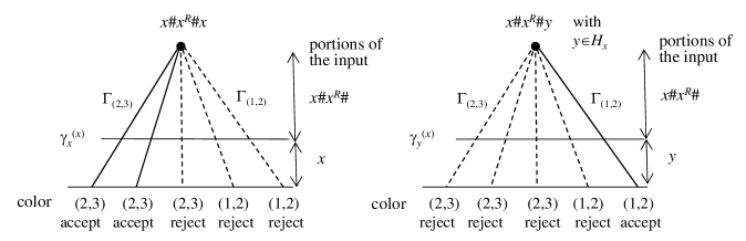
Figure 1: Two computation trees of the colored automaton $M$ on two inputs $x\#x^{R}x$ and $x\#x^{R}\#y$ with $y\in H_{x}$. The color of each computation path and its acceptance/rejection are written in the bottom of the figures.

Hereafter, let us focus on inputs of the form $x\#x^{R}\#y$ for $x,y\in\{0,1\}^{*}$. For any string $x\in\{0,1\}^{*}$, we abbreviate the set $\{y\in\{0,1\}^{|x|}\mid y\not\in\{x,x^{R}\}\}$ as $H_{x}$. Given a number $n\in\mathbb{N}^{+}$, $D^{(n)}_{(i,j)}$ denotes the set of all strings $x\in\{0,1\}^{n}$ for which there exists an accepting $(i,j)$-computation path of $M$ on input $x\#x^{R}\#x$. Since $g$ is single-valued, it follows that $D^{(n)}_{(1,2)}\cup D^{(n)}_{(2,3)}=\{0,1\}^{n}$. We therefore conclude that, for every length $n$, either $|D^{(n)}_{(1,2)}|\geq 2^{n}/2$ or $|D^{(n)}_{(2,3)}|\geq 2^{n}/2$ (or both) holds. We will discuss in Sections 3.3–3.5 the case where $|D_{(2,3)}^{(n)}|\geq 2^{n}/2$ holds for infinitely many $n$’s and consider in Section 3.6 the case where $|D_{(2,3)}^{(n)}|\geq 2^{n}/2$ holds only finitely many $n$’s (thus, $|D_{(1,2)}^{(n)}|\geq 2^{n}/2$ holds for infinitely many $n$’s). To complete the proof of Proposition 3.2, it suffices for us to obtain contradictions in both cases.

3.3 Case 1: $D^{(n)}_{(2,3)}$ is Large for Infinitely Many Lengths $n$

Let us first consider the case where the relation $|D^{(n)}_{(2,3)}|\geq 2^{n}/2$ holds for infinitely many lengths $n\in\mathbb{N}$. Take an arbitrary number $n\in\mathbb{N}$ that is significantly larger than $3^{|Q|+|\Sigma|+|\Gamma|}$ and also satisfies $|D^{(n)}_{(2,3)}|\geq 2^{n}/2$. We fix such a number $n$ throughout our proof and we thus tend to drop script “$n$” whenever its omission is clear from the context; for instance, we intend to write $D_{(2,3)}$ instead of $D^{(n)}_{(2,3)}$.

By the property of the colored automaton $M$ computing $g$, it follows that, for any pair $x,y\in\{0,1\}^{n}$, if $y\in H_{x}$ (i.e., $y\notin\{x,x^{R}\}$), then, for the input $x\#x^{R}\#y$, there always exists a certain accepting $(1,2)$-computation path of $M$. See Figure 1. However, since $g$ is single-valued, there must be no accepting $(1,2)$-computation path of $M$ on the input $x\#x^{R}\#x$ for every $x$ in $D_{(2,3)}$. In addition, no accepting $(1,2)$-computation path exists on all inputs of the form $x\#z\#y$ if $z\neq x^{R}$. Since there could be a large number of accepting $(1,2)$-computation paths of $M$ on $x\#x^{R}\#y$, we need to choose one of them arbitrarily and take a close look at this particular computation path.

For the aforementioned purpose, we denote by $PATH_{n}$ the set of all possible accepting $(1,2)$-computation paths of $M$ on inputs of the form $x\#x^{R}\#y$ for any two strings $x,y\in\{0,1\}^{n}$, and we fix a partial assignment $\pi:D_{(2,3)}\times\{0,1\}^{n}\rightarrow PATH_{n}$ that, for any element $(x,y)$, if $y\in H_{x}$, then $\pi$ picks one of the accepting $(1,2)$-computation paths of $M$ on the input $x\#x^{R}\#y$; otherwise, let $\pi(x,y)$ be undefined, for simplicity. Hereafter, we abbreviate $\pi(x,y)$ as $p_{x,y}$. Thus, $p_{x,y}$ is uniquely determined from $(x,y)$ whenever $\pi(x,y)$ is defined.

Along the unique accepting $(1,2)$-computation path $p_{x,y}$ of $M$ on each input $x\#x^{R}\#y$, the notation $\gamma^{(x)}_{i,y}$ is used to denote a stack content obtained by $M$ just after reading off the first $i$ symbols of $x\#x^{R}\#y$ (making all possible $\lambda$-moves). Note that, for each $x\in D_{(2,3)}$ and any $y\in H_{x}$, along the accepting $(1,2)$-computation path $p_{x,y}$ associated with the input $x\#x^{R}\#y$, $M$ produces unique stack contents $\gamma^{(x)}_{|x\#|,y}$ and $\gamma^{(x)}_{|x\#x^{R}\#|,y}$. For convenience, we abbreviate as $\gamma_{y}^{(x)}$ the stack content $\gamma^{(x)}_{|x\#x^{R}\#|,y}$, which is produced by $M$ just after reading the substring $x\#x^{R}\#$ of the input $x\#x^{R}\#y$.

In Sections 3.4–3.6, we plan to evaluate how many strings $x$ in $D_{(2,3)}$ satisfy each of the following conditions.

1. Strings $x$ make $\gamma_{y}^{(x)}$ small in size for all strings $y$ in $H_{x}$.

2. Strings $x$ make $\gamma_{y}^{(x)}$ relatively large in size for certain strings $y$ in $H_{x}$.

Proposition 3.7 gives a lower bound on the number of strings $x$ satisfying Condition (1), whereas Propositions 3.13 and 3.16 provide lower bounds on the number of strings $x$ for Condition (2). If these two bounds are large enough, then they guarantee the existence of a string that meet both conditions, clearly leading to a contradiction. Therefore, we conclude that $M$ cannot exist, closing Case 1. Proposition 3.7 will be verified in Section 3.4 and Propositions 3.13 and 3.16 will appear in Section 3.5.

3.4 Fundamental Properties of a Stack History

A key to our proof is an analysis of a stack history of the given colored automaton $M$. In the following series of lemmas and a proposition, we will explore fundamental properties of a stack history of $M$ along accepting $(1,2)$-computation path $p_{x,y}$ on any input of the form $x\#x^{R}\#y$. Those properties are essential in dealing with Case 1. We start with showing a simple property asserting that, in the above stack history, the same stack content does not appear twice or more.

Lemma 3.5

Fix $x\in D_{(2,3)}$ and $y\in\{0,1\}^{n}$ arbitrarily. For any accepting $(1,2)$-computation path $p_{x,y}$ of $M$ on the input $x\#x^{R}\#y$, there is no pair $(i_{1},i_{2})$ of cell positions satisfying that $|x|<i_{1}<i_{2}\leq|x\#x^{R}\#|$ and $\gamma^{(x)}_{i_{1},y}=\gamma^{(x)}_{i_{2},y}$. Moreover, the same statement is true when $1\leq i_{1}<i_{2}\leq|x|$.

Proof.    Assume that $M$ has an accepting $(1,2)$-computation path $p_{x,y}$ for the given strings $x\in D_{(2,3)}$ and $y\in\{0,1\}^{n}$. If the first part of the lemma fails, then the inequality $\gamma^{(x)}_{i_{1},y}=\gamma^{(x)}_{i_{2},y}$ must hold for a certain pair $(i_{1},i_{2})$ satisfying $|x|<i_{1}<i_{2}\leq|x\#x^{R}\#|$. We remove from $x\#x^{R}\#y$ all input symbols located in between cell positions $i_{1}+1$ and $i_{2}$ and then express the resulted string by $x\#x^{\prime}\#y$. Since $\gamma^{(x)}_{i_{1},y}=\gamma^{(x)}_{i_{2},y}$, we can obtain a new $(1,2)$-computation path, along which $M$ still enters an accepting state on this input $x\#x^{\prime}\#y$. However, since $x^{\prime}\neq x^{R}$, there must be no accepting $(1,2)$-computation path on $x\#x^{\prime}\#y$, a contradiction. The second part of the lemma follows by a similar argument. $\Box$

Lemma 3.5 can be generalized as follows.

Lemma 3.6

Let $x_{1},x_{2},y_{1},y_{2}\in\{0,1\}^{n}$ satisfy both $y_{1}\in H_{x_{1}}$ and $y_{2}\in H_{x_{2}}$ and let $i_{1},i_{2}\in\mathbb{N}$ satisfy $1\leq i_{1},i_{2}\leq|x_{1}\#x_{1}^{R}\#|$. Let $w_{1}=x_{1}\#x_{1}^{R}\#y_{1}$ and $w_{2}=x_{2}\#x_{2}^{R}\#y_{2}$. Assume that one of the following three conditions holds: (i) $i_{1}\neq i_{2}$, (ii) $1\leq i_{1}=i_{2}\leq|x_{1}\#|$ and $(w_{1})_{i_{1}}\neq(w_{2})_{i_{2}}$, and (iii) $|x_{1}\#|<i_{1}=i_{2}\leq|x_{1}\#x_{1}^{R}\#|$ and $(w_{1})_{i_{1}}\neq(w_{2})_{i_{2}}$. If the two computation paths $p_{x_{1},y_{1}}$ and $p_{x_{2},y_{2}}$ exist, then $\gamma^{(x_{1})}_{i_{1},y_{1}}\neq\gamma^{(x_{2})}_{i_{2},y_{2}}$ holds.

Proof.    Let $(x_{1},x_{2},y_{1},y_{2},i_{1},i_{2})$ be parameters given as in the premise of the lemma. We consider the three cases (i)–(iii) separately. The first case of $i_{1}\neq i_{2}$ comes from an argument similar to the proof of Lemma 3.5. In what follows, we therefore assume that $i_{1}=i_{2}$ and denote them as $i$ for simplicity.

Next, we consider the second case where $1\leq i\leq|x_{1}\#|$ and $(w_{1})_{i}\neq(w_{2})_{i}$. Toward a contradiction, we assume that $\gamma^{(x_{1})}_{i,y_{1}}=\gamma^{(x_{2})}_{i,y_{2}}$. Assume that there are two accepting $(1,2)$-computation paths $p_{x_{1},y_{1}}$ and $p_{x_{2},y_{2}}$ generated by $M$ respectively on the inputs $w_{1}$ and $w_{2}$. Notice that $i<|x_{1}|$ because, otherwise, $(w_{1})_{i}=(w_{2})_{i}$ follows. Take a unique nonempty string $u_{1}$ satisfying $x_{1}=(x_{1})_{i}u_{1}$. Since $\gamma^{(x_{1})}_{i,y_{1}}=\gamma^{(x_{2})}_{i,y_{2}}$ by our assumption, we can swap the initial segments of these two computation paths restricted to the first $i$ steps, corresponding to the first $i$ bits of the above two inputs. As a result, we obtain another accepting $(1,2)$-computation path on the input $(x_{2})_{i}u_{1}\#x_{1}^{R}\#y_{1}$. Since $M$ precisely computes $g$, $(x_{2})_{i}u_{1}$ must equal $x_{1}$. From this, $(w_{1})_{i}=(w_{2})_{i}$ follows instantly, a clear contradiction against $(w_{1})_{i}\neq(w_{2})_{i}$. Therefore, we obtain $\gamma^{(x_{1})}_{i,y_{1}}\neq\gamma^{(x_{2})}_{i,y_{2}}$.

A similar argument can handle the third case, in which both $|x_{1}\#|<i\leq|x_{1}\#x_{1}^{R}\#|$ and $(x_{1})_{i}\neq(x_{2})_{i}$ hold. Firstly, we claim that $x_{1}\neq x_{2}$ because, otherwise, $x_{1}\#x_{1}^{R}\#$ coincides with $x_{2}\#x_{2}^{R}\#$, contradicting $(w_{1})_{i}\neq(w_{2})_{i}$. Since $x_{1}\neq x_{2}$, we obtain $i<|x_{1}\#x_{1}^{R}|$. Take a unique string $u_{1}$ that satisfies $(x_{1}\#x_{1}^{R})_{i}u_{1}=x_{1}\#x_{1}^{R}$. Similarly to the second case, assuming $\gamma^{(x_{1})}_{i,y_{1}}=\gamma^{(x_{2})}_{i,y_{2}}$, there must exist an accepting $(1,2)$-computation path of $M$ on the input $(x_{2}\#x_{2}^{R})_{i}u_{1}\#y_{1}$. From this, we can draw a conclusion that $x_{2}^{R}u_{1}=x_{1}^{R}$; thus, $(w_{1})_{i}=(w_{2})_{i}$ follows, contradicting our assumption. $\Box$

In what follows, we want to estimate the number of strings $x$ in $D_{(2,3)}$ for which their corresponding stack contents $\gamma^{(x)}_{y}$ are small in size for an arbitrary string $y$ in $H_{x}$. In what follows, we will show its lower bound, which is sufficiently large.

Proposition 3.7

There exist two constants $d_{1},d_{2}\in\mathbb{N}^{+}$, independent of $(n,x,y)$, such that $|\{x\in D^{(n)}_{(2,3)}\mid\forall y\in H_{x}\,[|\gamma^{(x)}_{y}|<d_{1}]\}|\geq|D^{(n)}_{(2,3)}|-d_{2}$.

Proposition 3.7 is one of the key statements necessary to handle Case 1. For the proof of this proposition, we need two supporting lemmas, Lemmas 3.8 and 3.9. To explain these lemmas, we need to introduce extra terminology and notation.

Let us recall from Section 3.2 that $\{\Gamma_{t}\}_{y\in I_{3}}$ is a “color” partition of $\Gamma$. Given two strings $u\in(\Gamma_{(1,2)})^{+}$ and $v\in(\Gamma_{(1,2)})^{*}$ and a string $z\in\{0,1\}^{+}$, we say that $M$ transforms $u$ to $v$ while reading $z$ (along computation (sub)path $p$) if $M$ behaves as follows along this particular computation (sub)path $p$: (i) $M$ starts in inner state $q$ with $uw\bot$ in its stack for a certain string $w\in(\Gamma^{(1,2)})^{*}$, scanning the leftmost input symbol of $z$, (ii) $M$ then reads all input symbols in $z$, including no endmarker, one by one, (iii) just after reading off $z$ (making all possible $\lambda$-moves), $M$ enters inner state $q$, leaving $vw\bot$ in the stack, and (iv) $M$ does not access any symbol in $w$ while reading $z$. The notation $TF_{M}(u,v)$ expresses the set of all strings of the form $z\#z^{\prime}$ for any pair $z,z^{\prime}\in\{0,1\}^{*}$ such that $M$ transforms $u$ to $v$ while reading $z\#z^{\prime}$ along certain computation (sub)paths.

Lemma 3.8

Given any pair $u,v\in(\Gamma_{(1,2)})^{*}$, there exists at most one string $x^{\prime}$ such that $x^{\prime}$ is a substring of a certain string $x$ in $D_{(2,3)}$ and $M$ transforms $u$ to $v$ while reading $x^{\prime}$ along an appropriate subpath of $p_{x,y}$ for a certain string $y$ in $\{0,1\}^{n}$.

Proof.    We prove the lemma by way of contradiction. Assume that there are two distinct strings $x_{1},x_{2}\in\{0,1\}^{*}$ satisfying that $M$ transforms $u$ to $v$ while reading $x_{1}$ along computation subpath $p_{1}$ and $M$ transforms $u$ to $v$ while reading $x_{2}$ along computation subpath $p_{2}$. Let us consider a string $x$ in $D_{(2,3)}$ such that $x$ contains $x_{1}$ as a substring and an accepting $(1,2)$-computation path $p_{x,y}$ on input $x\#x^{R}\#y$ contains $p_{1}$ as a subpath for a certain string $y\in\{0,1\}^{n}$. Let $x^{\prime}$ be a string obtained from $x$ by replacing $x_{1}$ with $x_{2}$. It is possible to swap the two subpaths $p_{1}$ and $p_{2}$ without changing the acceptance criteria of $M$. Therefore, $M$ must have an accepting $(1,2)$-computation path on the input $x^{\prime}\#x^{R}\#y$. This is absurd since $x^{\prime}\neq x$. $\Box$

Next, we will show a technical lemma, Lemma 3.9, which is essential to prove Proposition 3.7. We already know from Lemma 3.5 that all elements in $\{\gamma^{(x)}_{i,y}\mid 1\leq i\leq|x\#x^{R}\#|\}$ are mutually distinct. Let us concentrate particularly on stack contents $\gamma^{(x)}_{i,y}$ of minimal size. Given any pair $(x,y)$, we define $MSC_{x,y}$ (minimal stack contents) to be the collection of all stack contents $\gamma$ that meet the following requirement: there exists a cell position $\ell$ with $|x\#|\leq\ell\leq|x\#x^{R}\#|$ such that (i) $\gamma=\gamma^{(x)}_{\ell,y}$ and (ii) $|\gamma|\leq|\gamma^{(x)}_{\ell^{\prime},y}|$ holds for any cell position $\ell^{\prime}$ satisfying $|x\#|\leq\ell^{\prime}\leq|x\#x^{R}\#|$. Condition (ii), in particular, ensures that the size of $\gamma$ must be minimum. Note that $MSC_{x,y}$ cannot be empty.

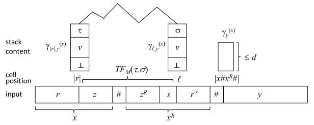
Figure 2: A stack history stated in Lemma 3.9.

Lemma 3.9

There exists a constant $d>0$, independent of $(n,x,y)$, that satisfies the following statements. Let $x\in D^{(n)}_{(2,3)}$, $y\in H_{x}$, and $\gamma^{(x)}_{\ell,y}\in MSC_{x,y}$ satisfying $|x\#|\leq\ell\leq|x\#x^{R}\#|$. Moreover, let $x=rz$, $x^{R}=z^{R}sr^{\prime}$, $\ell=|x\#z^{R}s|$, $\gamma^{(x)}_{|r|,y}=\tau v\bot$, and $\gamma^{(x)}_{\ell,y}=\sigma v\bot$ for an appropriate tuple $(r,r^{\prime},z,s,\sigma,\tau,v)$. If $\ell\neq|x\#|$ and $z\#z^{R}s\in TF_{M}(\tau,\sigma)$, then $|\gamma^{(x)}_{y}|\leq d$ holds. Moreover, when $n$ is sufficiently large, $\ell\neq|x\#|$ also holds.

Lemma 3.9 roughly states that, if there is an interval between $1$ and $|x\#x^{R}\#|$ crossing over the first $\#$ in which $M$ transforms a stack symbol $\tau$ to another $\sigma$, the size of stack content is small at the $|x\#x^{R}\#|$-th cell position. Figure 2 illustrates a stack history stated in the lemma.

Using Lemma 3.9, we can prove Proposition 3.7 in the following manner. Since $MSC_{x,y}$ is nonempty, we can take an element $\gamma^{(x)}_{\ell,y}$ from $MSC_{x,y}$ satisfying $|x\#|\leq\ell\leq|x\#x^{R}\#|$. By the size-minimality of $\gamma^{(x)}_{\ell,y}$, it follows that $|\gamma^{(x)}_{i,y}|\geq|\gamma^{(x)}_{\ell,y}|$ for any cell position $i$ with $|x\#|\leq i\leq\ell$. Since $M$ pushes at most one extra stack symbol into the stack, there must be a cell position $i$ satisfying both $1\leq i\leq|x\#|$ and $|\gamma^{(x)}_{i,y}|=|\gamma^{(x)}_{\ell,y}|$. This indicates that, by choosing an appropriate tuple $(r,r^{\prime},z,s,\sigma,\tau,u,v)$, we can decompose $x\#x^{R}\#y$ into

• $x=rz$, $x^{R}=z^{R}sr^{\prime}$, $\ell=|x\#z^{R}s|$, $\gamma^{(x)}_{|r|,y}=\tau v\bot$, $\gamma^{(x)}_{\ell,y}=\sigma v\bot$, and $z\#z^{R}s\in TF_{M}(\tau,\sigma)$.

The second part of Lemma 3.9 implies that, except for a finite number of $x$’s, $\ell\neq|x\#|$ always holds. We define $d_{2}$ to be the total number of those exceptional $x$’s. For the other $x$’s, since $\ell\neq|x\#|$, the first part of Lemma 3.9 then provides the desired constant $d_{1}$ that upper-bounds $|\gamma^{(x)}_{y}|$. We therefore obtain the proposition.

Now, it is time to verify Lemma 3.9. This lemma requires two additional lemmas, Lemmas 3.10 and 3.11. In the first lemma given below, we want to show that the size of $s$ in (*) is bounded from above by a certain absolute constant.

Lemma 3.10

There exists a constant $d_{1}>0$, independent of $(n,x,y)$, satisfying the following statements. Let $x\in D^{(n)}_{(2,3)}$, $y\in H_{x}$, and $\gamma^{(x)}_{\ell,y}\in MSC_{x,y}$ with $|x\#|\leq\ell\leq|x\#x^{R}\#|$. Moreover, let $x=rz$, $x^{R}=z^{R}sr^{\prime}$, $\ell=|x\#z^{R}s|$, $\gamma^{(x)}_{|r|,y}=\tau v\bot$, and $\gamma^{(x)}_{\ell,y}=\sigma v\bot$. If $\ell\neq|x\#|$ and $z\#z^{R}s\in TF_{M}(\tau,\sigma)$, then $|s|\leq d_{1}$ holds.

Proof.    Let $(r,r^{\prime},z,s,\sigma,\tau,u,v)$ satisfy that $x=rz$, $x^{R}=z^{R}sr^{\prime}$, $\ell=|x\#z^{R}s|$, $\gamma^{(x)}_{|r|,y}=\tau v\bot$, and $\gamma^{(x)}_{\ell,y}=\sigma v\bot$. Moreover, we assume that $\ell\neq|x\#|$ and $z\#z^{R}s$ belongs to $TF_{M}(\tau,\sigma)$. From the inequality $\ell\neq|x\#|$, it follows that $z^{R}s\neq\lambda$. Let us assume further that $\gamma^{(x)}_{\ell,y}\in MSC_{x,y}$. We first claim that the string $s$ can be uniquely determined from the pair $(\tau,\sigma)$.

Claim 1

Let $z_{1}\in\{0,1\}^{+}$ and $s_{1}\in\{0,1\}^{*}$ be arbitrary strings. If $z_{1}\#z_{1}^{R}s_{1}\in TF_{M}(\tau,\sigma)$, then $s=s_{1}$ holds.

Claim 1 uniquely associates $s$ with $(\tau,\sigma)$, and thus we can define a map from $(\tau,\sigma)$ to $s$. Hence, the number of all possible strings $s$ is at most $|\Gamma^{\prime}_{(1,2)}|^{2}$, which is obviously a constant. From this fact, we can draw a conclusion that $|s|$ is upper-bounded by an appropriately chosen constant, independent of $(n,x,y)$.

Finally, let us prove Claim 1. Toward a contradiction, we assume that $z_{1}\#z_{1}^{R}s_{1}\in TF_{M}(\tau,\sigma)$ and $s\neq s_{1}$. Let $p_{1}$ denote any accepting $(1,2)$-computation path generated by $M$ while reading off $rz\#z^{R}sr^{\prime}\#y$. Consider its computation subpath, say, $p_{2}$ associated with the substring $z\#z^{R}s$. By our assumption of $z_{1}\#z_{1}^{R}s_{1}\in TF_{M}(\tau,\sigma)$, there exists a computation subpath, say, $p_{3}$ corresponding to $z_{1}\#z_{1}^{R}s_{1}$. Now, along the computation path $p_{1}$, we replace the subpath $p_{2}$ by $p_{3}$. This produces a new accepting $(1,2)$-computation path on the input $rz_{1}\#z_{1}^{R}s_{1}r^{\prime}\#y$. Thus, we conclude that $(rz_{1})^{R}=z_{1}^{R}r^{R}=z_{1}^{R}sr^{\prime}\neq z_{1}^{R}s_{1}r^{\prime}$ because of $s\neq s_{1}$. This means that there is no accepting $(1,2)$-computation path on $rz_{1}\#z_{1}^{R}s_{1}r^{\prime}\#y$, a contradiction. Therefore, Claim 1 is true. $\Box$

In the second lemma below, we want to show that the size of $r^{\prime}$ in (*) is also upper-bounded by a certain absolute constant.

Lemma 3.11

There exists a constant $d_{2}>0$, independent of $(n,x,y)$, that satisfies the following statements. Let $x\in D^{(n)}_{(2,3)}$, $y\in H_{x}$, and $\gamma^{(x)}_{\ell,y}\in MSC_{x,y}$. Moreover, let $x=rz$, $x^{R}=z^{R}sr^{\prime}$, $y=r^{\prime\prime}z^{\prime}$, $\ell=|x\#z^{R}s|$, $\ell^{\prime}=|x\#x^{R}\#r^{\prime\prime}|$, $\gamma^{(x)}_{|r|,y}=\tau v\bot$, $\gamma^{(x)}_{\ell,y}=\sigma v\bot$, and $\gamma^{(x)}_{\ell^{\prime},y}=v\bot$. If $r^{\prime}\#r^{\prime\prime}\in TF_{M}(\sigma,\lambda)$, then $|r^{\prime}|\leq d_{2}$ holds.

Proof.    Take parameters $(r,r^{\prime},r^{\prime\prime},z,z^{\prime},u,\tau,\sigma,\ell,\ell^{\prime})$ as specified in the premise of the lemma and assume that $r^{\prime}\#r^{\prime\prime}\in TF_{M}(\sigma,\lambda)$. Similarly to Claim 1, we claim that $\sigma$ uniquely determines $r^{\prime}$.

Claim 2

Let $r^{\prime}_{1},r^{\prime\prime}_{1}\in\{0,1\}^{*}$. If $r^{\prime}_{1}\#r^{\prime\prime}_{1}\in TF_{M}(\sigma,\lambda)$, then $r^{\prime}_{1}=r^{\prime}$.

Claim 2 helps us define a map from $\sigma$ to $r^{\prime}$ since $r^{\prime}$ is uniquely determined by $\sigma$. This mapping implies that the number of all possible $r^{\prime}$ is at most $|\Gamma^{\prime}_{(1,2)}|$. Since there are at most $|\Gamma^{\prime}_{(1,2)}|$ such strings $r^{\prime}$, $|r^{\prime}|$ must be bounded from above by a certain constant, independent of $(n,x,y)$.

Claim 2 itself can be proven by way of contradiction. First, we assume that $r^{\prime}_{1}\neq r^{\prime}$. Since $y\in H_{x}$, we are focused on the accepting $(1,2)$-computation path $p_{x,y}$ on the input $x\#x^{R}\#y$, which equals $rz\#z^{R}sr^{\prime}\#r^{\prime\prime}z^{\prime}$. Since $r^{\prime}\#r^{\prime\prime}\in TF_{M}(\sigma,\lambda)$ and $r^{\prime}_{1}\#r^{\prime\prime}_{2}\in TF_{M}(\sigma,\lambda)$, we can replace its subpath associated with $r^{\prime}\#r^{\prime\prime}$ by a subpath generated by $M$ while reading off $r^{\prime}_{1}\#r^{\prime\prime}_{1}$. We then obtain another accepting $(1,2)$-computation path on the input $x\#z^{R}sr^{\prime}_{1}\#r^{\prime\prime}_{1}z^{\prime}$. By the definition of $h_{3}$ and the choice of $M$, $x^{R}=z^{R}sr^{\prime}_{1}$ must hold. On the contrary, we obtain $x^{R}=z^{R}sr^{\prime}\neq z^{R}sr^{\prime}_{1}$ from $r^{\prime}_{1}\neq r^{\prime}$. This is a contradiction. $\Box$

Finally, we are ready to prove Lemma 3.9 with the help of Lemmas 3.10 and 3.11.

Proof of Lemma 3.9.   Let $(r,r^{\prime},z,s,\sigma,\tau,v,y)$ be given as in the premise of the lemma. Notice that $x=rz$, $x^{R}=z^{R}sr^{\prime}$, and $\gamma^{(x)}_{\ell,y}=\sigma v\bot$ with $\ell=|x\#z^{R}s|$. Since $\gamma^{(x)}_{\ell,y}\in MSC_{x,y}$, there exists a nonempty string $u$ satisfying $\gamma^{(x)}_{y}=uv\bot$. Assume that $M$ transforms $\sigma$ to $u$ while reading $r^{\prime}$.

We first claim that $\ell\neq|x\#|$ for any sufficiently large $n$. Assume otherwise; namely, $\ell=|x\#|$. This assumption yields $z=s=\lambda$, which implies that $x=rz=r$ and $x^{R}=z^{R}sr^{\prime}=r^{\prime}$. In this case, for a certain string $r^{\prime\prime}$, it follows that $x^{R}\#r^{\prime\prime}\in TF_{M}(\sigma,\tau)$ and $\gamma^{(x)}_{\ell^{\prime},y}=v\bot$, where $\ell^{\prime}=|x\#x^{R}\#r^{\prime\prime}|$. By Lemma 3.11, we obtain a constant size-upper bound of $r^{\prime}$; in other words, there exists a constant $d_{2}$, independent of $(n,x,y)$, satisfying $|r^{\prime}|\leq d_{2}$. Since $n=|x|$ is sufficiently large, $r^{\prime}$ must be large in size as well. This is a contradiction. Therefore, $\ell\neq|x\#|$ holds.

Hereafter, we assume that $\ell\neq|x\#|$ and $z\#z^{R}s\in TF_{M}(\tau,\sigma)$. Lemma 3.10 further ensures the existence of an appropriate constant $d_{1}$ for which $|s|\leq d_{1}$. Lemma 3.11 also shows that $|r^{\prime}|$ is upper-bounded by a certain constant, say, $d_{2}$. Since $|r|=|sr^{\prime}|=|s|+|r^{\prime}|$ by definition, $|r|$ is bounded from above by $d_{1}+d_{2}$. Let $\sigma_{0}$ be the stack symbol pushed into the stack at the first step of $M$. Since $M$ transforms $\sigma_{0}$ to $\tau v$ while reading $r$ for a certain stack symbol $\tau$ and the stack increases by at most one, it follows that $|v|$ is upper-bounded by a certain absolute constant. Therefore, since $|r^{\prime}|\leq d_{2}$, $|uv\bot|$ is bounded as well. $\Box$

We have completed the proof of Proposition 3.7. As a preparation for a further discussion on Case 1, we provide a useful lemma, which will be used in Section 3.5.

Lemma 3.12

Let $x_{1},x_{2},y\in\{0,1\}^{n}$ with $x_{2}\in H_{x_{1}}$ and $y\in H_{x_{2}}$. If $x_{2}\in D_{(2,3)}$ and $x_{1}\neq x_{2}$, then there is no cell position $i$ for which $|x_{1}|\leq i\leq|x_{1}\#x_{1}^{R}\#|$ and $\gamma^{(x_{1})}_{i,x_{2}}=\gamma^{(x_{2})}_{i,y}$.

Proof.    Assume that $x_{2}\in D_{(2,3)}$ and $x_{1}\neq x_{2}$. To lead to a contradiction, we further assume that a position $i$ in the lemma actually exists. Let $j=|x_{1}\#x_{1}^{R}\#|-i$. Now, let us consider two accepting $(1,2)$-computation paths $p_{x_{1},x_{2}}$ and $p_{x_{2},y}$. Since $\gamma^{(x_{1})}_{i,x_{2}}=\gamma^{(x_{2})}_{i,y}$, it is possible to swap between subpaths of $p_{x_{1},x_{2}}$ and $p_{x_{2},y}$ generated by $M$ while reading substrings $x_{1}\#(x_{1}^{R})_{j}$ and $x_{2}\#(x_{2}^{R})_{j}$, respectively. We then obtain another accepting $(1,2)$-computation path, say, $p$ on the input $x_{2}\#(x_{2}^{R})_{j}(x_{1}^{R})_{n-j}\#x_{2}$. Here, we handle two possible cases.

(Case i) If $(x_{2}^{R})_{j}(x_{1}^{R})_{n-j}\neq x_{2}^{R}$, then the computation path $p$ cannot be an accepting $(1,2)$-computation path, a contradiction.

(Case ii) If $(x_{2}^{R})_{j}(x_{1}^{R})_{n-j}=x_{2}^{R}$, then $x_{2}\#(x_{2}^{R})_{j}(x_{1}^{R})_{n-j}\#x_{2}$ equals $x_{2}\#x_{2}^{R}\#x_{2}$. The obtained computation path $p$ is indeed an accepting $(1,2)$-computation path on $x_{2}\#x_{2}^{R}\#x_{2}$, and thus $x_{2}$ must be in $D_{(1,2)}$. This obviously contradicts the choice of $x_{2}\in D_{(2,3)}$, a contradiction. $\Box$

3.5 Size of Stack Contents

We continue our discussion on Case 1. In Proposition 3.7, we have shown that all but a constant number of strings $x$ in $D_{(2,3)}$ satisfy the inequality $|\gamma^{(x)}_{y}|<d_{1}$ for all strings $y$ in $H_{x}$. Toward an intended contradiction, we will further show that there are a large portion of $x$’s in $D_{(2,3)}$ whose corresponding stack contents $\gamma^{(x)}_{y}$ for appropriately chosen strings $y$ are large in size. Together with Proposition 3.7, we can derive the desired contradiction.

In the subsequent argument, the notation $E_{x}$ expresses the collection of all stack contents $\gamma^{(x)}_{y}$ at the $|x\#x^{R}\#|$-th cell position (obtained just after reading off $x\#x^{R}\#$) along an accepting $(1,2)$-computation path $p_{x,y}$ of $M$ on input $x\#x^{R}\#y$ for each string $y\in H_{x}$. Since $\pi$ is fixed, it follows that $1\leq|E_{x}|\leq|H_{x}|=2^{|x|}-2$ because there are at most $|H_{x}|$ subpaths generated by $M$ while reading inputs $x\#x^{R}\#y$ with $y\in H_{x}$.

Prior to a discussion on a general case of $|E_{x}|\geq 1$, we wish to consider a special case where $|E_{x}|$ equals $1$ for any string $x\in D_{(2,3)}$, because this case exemplifies an essence of our proof for the general case.

I) Special Case of $|E_{x}|=1$.

Since $|E_{x}|=1$, the choice of $y\in H_{x}$ becomes irrelevant. It is thus possible to drop subscript “$y$” altogether and abbreviate, e.g., $\gamma^{(x)}_{i,y}$, $\gamma^{(x)}_{y}$, and $u_{x,y}$ as $\gamma^{(x)}_{i}$, $\gamma^{(x)}$, and $u_{x}$, respectively. To lead to the desired contradiction, we want to show in Proposition 3.13 that a large number of strings $x$ in $D_{(2,3)}$ produce stack contents $\gamma^{(x)}_{y}$ of extremely large size for certain strings $y\in H_{x}$. Now, recall the notation $\Gamma^{\prime}_{(1,2)}$ that stands for the set $\Gamma_{(1,2)}\cup\{\bot\}$.

Proposition 3.13

Given any number $\epsilon\geq 0$, it follows that $|\{x\in D_{(2,3)}\mid\exists y\in H_{x}\,[|\gamma^{(x)}_{y}|\geq(n-2-\epsilon)/\log|\Gamma^{\prime}_{(1,2)}|]\}|\geq|D_{(2,3)}|(1-2^{-\epsilon})$.

To prove Proposition 3.13, let us consider two stack contents $\gamma^{(x_{1})}_{x_{2}}$ and $\gamma^{(x_{2})}_{x_{1}}$ associated with two distinct strings $x_{1},x_{2}\in D_{(2,3)}$. By choosing $i=|x_{1}\#x_{1}^{R}\#|$ in Lemma 3.12, we immediately obtain $\gamma^{(x_{1})}_{x_{2}}\neq\gamma^{(x_{2})}_{x_{1}}$. We then reach the following conclusion.

Lemma 3.14

For every distinct pair $x_{1}$ and $x_{2}$ in $D_{(2,3)}$, it follows that $\gamma^{(x_{1})}\neq\gamma^{(x_{2})}$.

To simplify our notation further, we write $A_{d}$ to express the set $\{x\in D_{(2,3)}\mid\exists y\in H_{x}\,[|\gamma^{(x)}_{y}|\geq d]\}$ for each chosen number $d\in\mathbb{N}^{+}$. With this notation, Proposition 3.13 is equivalent to the assertion that $|A_{(n-2-\varepsilon)/\log|\Gamma^{\prime}_{(1,2)}|}|\geq|D_{(2,3)}|(1-2^{-\varepsilon})$. Associated with $A_{d}$, we define $B_{d}=\{x\in D_{(2,3)}\mid\forall y\in H_{x}\,[|\gamma^{(x)}_{y}|<d]\}$. Note that $D_{(2,3)}=A_{d}\cup B_{d}$ and $A_{d}\cap B_{d}=\emptyset$ for any number $d\in\mathbb{N}^{+}$. In the following lemma, we present a lower bound on the cardinality of $A_{d}$.

Lemma 3.15

For any constant $d\in\mathbb{N}^{+}$, it follows that $|A_{d}|\geq|D_{(2,3)}|-2|\Gamma^{\prime}_{(1,2)}|^{d}$.

Proof.    Since $\{A_{d},B_{d}\}$ partitions $D_{(2,3)}$, it follows that $|A_{d}|=|D_{(2,3)}|-|B_{d}|$. To prove the lemma, let us concentrate on $B_{d}$. From $|E_{x}|=1$, $B_{d}$ coincides with $\{x\in D_{(2,3)}\mid|\gamma^{(x)}|<d\}$. Notice that each $\gamma^{(x)}$ belongs to $(\Gamma^{\prime}_{(1,2)})^{m}$ for a certain number $m$ with $m\leq d-1$. Consider a mapping $h$ from $x$ to $\gamma^{(x)}$. Induced from $B_{d}$, we define $\bar{B}_{d}=\{x\in B_{d}\mid x^{R}=x\}$. The function $h$ is 1-to-1 on $\bar{B}_{d}$ and, by Lemma 3.14, it is also 1-to-1 on at least a half of elements in $B_{d}-\bar{B}_{d}$. Hence, it follows that $|B_{d}|/2\leq\sum_{j=0}^{d-1}|\Gamma^{\prime}_{(1,2)}|^{j}=|\Gamma^{\prime}_{(1,2)}|^{d}$. We conclude that $|A_{d}|=|D_{(2,3)}|-|B_{d}|\geq|D_{(2,3)}|-2|\Gamma^{\prime}_{(1,2)}|^{d}$, as requested. $\Box$

With the help of Lemma 3.15, Proposition 3.13 is now easy to prove.

Proof of Proposition 3.13.   For simplicity, we use $d$ to denote $(n-2-\epsilon)/\log|\Gamma^{\prime}_{(1,2)}|$, which equals $\log_{|\Gamma^{\prime}_{(1,2)}|}2^{n-2-\epsilon}$. Our goal is to show that $|A_{d}|\geq|D_{(2,3)}|(1-2^{-\epsilon})$. By Lemma 3.15, we obtain $|A_{d}|\geq|D_{(2,3)}|-2|\Gamma^{\prime}_{(1,2)}|^{d}$. Notice that, by the definition, $|\Gamma^{\prime}_{(1,2)}|^{d}=2^{n-2-\varepsilon}\leq|D_{(2,3)}|\cdot 2^{-1-\varepsilon}$, where the last inequality comes from our assumption of $|D_{(2,3)}|\geq 2^{n}/2$. As a result, we obtain $|A_{d}|\geq|D_{(2,3)}|-2|\Gamma^{\prime}_{(1,2)}|^{d}\geq|D_{(2,3)}|(1-2^{-\epsilon})$, as requested. $\Box$

To finish this special case, let $x=rz$, $x^{R}=z^{R}sr^{\prime}$, $\gamma^{(x)}=uv\bot$, and $\gamma^{(x)}_{\ell}=\sigma v\bot$ with $\ell=|x\#z^{R}s|$. Assume that $M$ transforms $\sigma$ to $u$ while reading $r^{\prime}$. Proposition 3.7 shows that, for most of $x$’s, $|uv\bot|$ is upper-bounded by a certain constant, independent of $(n,x,y)$. However, by setting, e.g.,  $\epsilon=98$, Proposition 3.13 yields $|uv\bot|\geq(n-100)/\log|\Gamma^{\prime}_{(1,2)}|$ for at least the $2/3$-fraction of $x$’s in $D_{(2,3)}$. Since $n$ is sufficiently large, $|uv\bot|$ cannot be bounded from above by any absolute constant. Therefore, we obtain a clear contradiction.

II) General Case of $|E_{x}|\geq 1$.

We have already shown how to cope with the case of $|E_{x}|=1$ for all strings $x\in D_{(2,3)}$. Hereafter, we will discuss a general case where $|E_{x}|\geq 1$ holds for any $x\in D_{(2,3)}$. Our goal is to prove the correctness of the following statement.

Proposition 3.16

Let $d>0$. All but $2(|\Gamma^{\prime}_{(1,2)}|^{d}+1)$ strings $x$ in $D_{(2,3)}$ satisfy the following: there exists a stack content $\tau\in E_{x}$ for which $\tau$ contains at least $d$ symbols; namely, $|\{x\in D_{(2,3)}\mid\exists\,\tau\in E_{x}\,[|\tau|\geq d]\}|\geq|D_{(2,3)}|-2|\Gamma^{\prime}_{(1,2)}|^{d}-2$.

We first give basic notions and notation needed for the proof of Proposition 3.16. With a fixed number $n$, let $G_{n}$ denote a specific undirected graph $(V_{n},E_{n})$ in which $V_{n}=\{(i,j)\mid i,j\in[n],i\neq j\}$ and, for any two vertices $v_{1}=(i_{1},j_{1})$ and $v_{2}=(i_{2},j_{2})$ in $V_{n}$, $(v_{1},v_{2})$ belongs to $E_{n}$ if either $i_{1}=j_{2}$ or $i_{2}=j_{1}$. A coloring of $G_{n}$ is a function $\phi:V_{n}\to C$ for a certain finite set $C$. Given a number $t\in\mathbb{N}^{+}$, $G_{n}$ is said to be $t$-colorable if there exists a coloring $\phi:V_{n}\to C$ with $|C|=t$ for which no single color is assigned to two adjacent vertices (i.e., no edge $(v_{1},v_{2})\in E$ satisfies $\phi(v_{1})=\phi(v_{2})$). The chromatic number of $G_{n}$, denoted by $\chi(G_{n})$, is the smallest number $t\in\mathbb{N}^{+}$ that makes $G_{n}$ be $t$-colorable.

Lemma 3.17

For any $n\in\mathbb{N}^{+}$ with $n\geq 3$, $\chi(G_{n})$ equals $n$.

Proof.

Firstly, we assert that $\chi(G_{n})\leq n$. To achieve this goal, we define a special coloring $\phi$ as follows. Let $C$ be the color set $\{c_{1},c_{2},\ldots,c_{n}\}$. For any pair $i,j\in[n]$ with $i\neq j$, we set $\phi((i,j))=c_{j}$. It then follows that, for any two distinct vertices $v_{1}=(i_{1},j_{1})$ and $v_{2}=(i_{2},j_{2})$ in $G_{n}$, if $\phi(v_{1})=\phi(v_{2})$, then $j_{1}=j_{2}$ holds; thus, we obtain $(v_{1},v_{2})\notin E_{n}$ because, otherwise, either $i_{1}=j_{1}$ or $i_{2}=j_{2}$ follows. Therefore, $\phi$ is a valid coloring of $G_{n}$. Since $|C|=n$, we obtain $\chi(G_{n})\leq n$.

To show that $\chi(G_{n})\geq n$, on the contrary, we start with calculating the “independent number” of $G_{n}$. An independent set $A$ of $G_{n}$ is a set of vertices of $G_{n}$ such that any two distinct vertices in $A$ cannot be adjacent in $G_{n}$. The independent number $\alpha(G_{n})$ is the maximum size of any independent set of $G_{n}$. It is immediate that $\chi(G_{n})\alpha(G_{n})\geq|V|$. We estimate $\alpha(G_{n})$ in the following claim.

Claim 3

For each $n\in\mathbb{N}^{+}$ with $n\geq 3$, $\alpha(G_{n})=n-1$.

From this claim, since $|V_{n}|=n(n-1)$ and $\alpha(G_{n})=n-1$, we conclude that $\chi(G_{n})\geq\frac{|V_{n}|}{\alpha(G_{n})}=\frac{n(n-1)}{n-1}=n$, as requested.

To prove Claim 3, we first show that $\alpha(G_{n})\geq n-1$. For this purpose, let us consider the set $A=\{(1,i)\in V_{n}\mid i\in[2,n]_{\mathbb{Z}}\}$. Clearly, $A$ is an independent set of $G_{n}$. Since $|A|=n-1$, we immediately obtain $\alpha(G_{n})\geq n-1$. Next, we intend to verify that $\alpha(G_{n})\leq n-1$. Toward a contradiction, we assume that $\alpha(G_{n})\geq n$. Take an independent set, say, $B$ of $G_{n}$ of cardinality $n$. We assume that $B$ has the form $\{(k_{i},j_{i})\mid i\in[n]\}$. Since $|B|=n$, it is not difficult to show that there are two numbers $i_{1},i_{2}\in[n]$ for which either $k_{i_{1}}=j_{i_{2}}$ or $k_{i_{2}}=j_{i_{1}}$ holds. This is a contradiction. Thus, we conclude that $\alpha(G_{n})\leq n-1$. This completes the proof of the claim. ∎

Let us return to the proof of Proposition 3.16.

Proof of Proposition 3.16.   As done in I), we set $A_{d}=\{x\in D_{(2,3)}\mid\exists y\in H_{x}\,[|\gamma^{(x)}_{y}|\geq d]\}$ and define $B_{d}=\{x\in D_{(2,3)}\mid\forall y\in H_{x}\,[|\gamma^{(x)}_{y}|<d]\}$ so that $D_{(2,3)}=A_{d}\cup B_{d}$. With these notations, the proposition asserts that $|A_{d}|\geq|D_{(2,3)}|-2(|\Gamma^{\prime}_{(1,2)}|^{d}+1)$, or equivalently, $|B_{d}|\leq 2(|\Gamma^{\prime}_{(1,2)}|^{d}+1)$. We further restrict $B_{d}$ as $\hat{B}_{d}=\{x\in B_{d}\mid x<x^{R}\}$, where “$<$” is the lexicographic ordering on $\{0,1\}^{n}$. Obviously, $|B_{d}|\leq 2|\hat{B}_{d}|$ follows. To obtain the proposition, it therefore suffices to prove the statement: (*) $|\hat{B}_{d}|\leq|\Gamma^{\prime}_{(1,2)}|^{d}+1$. In what follows, we wish to prove this statement (*).

Let $m=|\hat{B}_{d}|$ for simplicity. We express all elements of $\hat{B}_{d}$ as $\{x_{1},x_{2},\ldots,x_{m}\}$ and then identify it with the integer set $\{1,2,\ldots,m\}$ ($=[m]$). We then introduce an undirected graph $G=(V,E)$ as follows. Let $V=\{(x,y)\mid x,y\in[m],x\neq y\}$ and define $E$ to be composed of all edges $((x_{1},x_{2}),(x_{2},y_{2}))$ such that (i) $(x_{1},y_{1}),(x_{2},x_{2})\in V$ and (ii) either $x_{1}=y_{2}$ or $x_{2}=y_{1}$. We set $C=\{\gamma^{(x)}_{y}\mid(x,y)\in V\}$ and define a function $\phi:V\to C$ by setting $\phi(x,y)=\gamma^{(x)}_{y}$, where $x$ and $y$ are seen as associated elements in $\hat{B}_{d}$. We assert the following claim concerning $\phi$.

Claim 4

For any $x,y,z$, if $(x,y)$ and $(y,z)$ are vertices in $V$, then $\phi(x,y)\neq\phi(y,z)$ holds.

To prove the claim, we assume otherwise. Take three elements $x,y,z$ satisfying that $(x,y),(y,z)\in V$ and $\phi(x,y)=\phi(y,z)$. Note that $x,y\in D_{(2,3)}$, $y\in H_{x}$, and $z\in H_{y}$. By Lemma 3.12 with $i=|x\#x^{R}\#|$, we conclude that $\gamma^{(x)}_{i,y}\neq\gamma^{(y)}_{i,z}$. From this inequality, we obtain $\phi(x,y)\neq\phi(y,z)$. However, this is obviously a contradiction. Therefore, the claim is true.

By Claim 4, $\phi$ turns out to be a coloring of $G$; thus, we obtain $\chi(G)\leq|C|$. Since $C\subseteq(\Gamma^{\prime}_{(1,2)})^{<d}$, it follows that $\chi(G)\leq|C|\leq\sum_{i=0}^{d-1}|\Gamma^{\prime}_{(1,2)}|^{i}=|\Gamma^{\prime}_{(1,2)}|^{d}$. Furthermore, Lemma 3.17 implies that the chromatic number of $G$ is exactly $m-1$, which equals $|\hat{B}_{d}|-1$. Thus, we conclude that $|\hat{B}_{d}|\leq|C|+1\leq|\Gamma^{\prime}_{(1,2)}|^{d}+1$, as requested. $\Box$

Finally, let us close Case 1 by drawing a contradiction. Here, we set $d=\lfloor\log_{|\Gamma|}(|D_{(2,3)}|/8)\rfloor$. A simple calculation yields $2(|\Gamma^{\prime}_{(1,2)}|^{d}+1)\leq 4|\Gamma^{\prime}_{(1,2)}|^{d}\leq|D_{(2,3)}|/2$. Moreover, since $|D_{(2,3)}|\geq 2^{n}/2$, it follows that $d\geq\log_{|\Gamma^{\prime}_{(1,2)}|}\frac{|D_{(2,3)}|}{8}-1\geq\frac{n-4}{\log{|\Gamma^{\prime}_{(1,2)}|}}-1$. By Proposition 3.16, for at least $|D_{(2,3)}|-2|\Gamma^{\prime}_{(1,2)}|^{d}-2$ ($\geq|D_{(2,3)}|/2$) elements $x$ in $D_{(2,3)}$, an appropriately chosen string $y\in H_{x}$ makes $\gamma^{(x)}_{y}$ satisfy $|\gamma^{(x)}_{y}|\geq d$, which further implies $|\gamma^{(x)}_{y}|\geq(n-4)/\log{|\Gamma^{\prime}_{(1,2)}|}-1$. Proposition 3.7, however, indicates that, except for at most $d_{2}$ elements in $D_{(2,3)}$, all strings $x\in D_{(2,3)}$ satisfy $|\gamma^{(x)}_{y}|\leq d_{1}$ for any choice of $y$ in $H_{x}$, where $d_{1}$ and $d_{2}$ are absolute constants, not depending on $(n,x,y)$. Since there are infinitely many $n$ satisfying $|D_{(2,3)}|\geq 2^{n}/2$, for any sufficiently large $n$, there exists a string $x\in D_{(2,3)}$ for which $|\gamma^{(x)}_{y}|\geq(n-4)/\log|\Gamma^{\prime}_{(1,2)}|-1$ and $|\gamma^{(x)}_{y}|\leq d_{1}$. This leads to a clear contradiction, as requested; therefore, this closes Case 1.

3.6 Case 2: $D^{(n)}_{(1,2)}$ is Large for Infinitely Many Lengths $n$

We have already handled Case 1 in Sections 3.3–3.5. To complete the proof of Proposition 3.2, nevertheless, we still need to deal with the remaining second case where $\{n\in\mathbb{N}^{+}\mid|D^{(n)}_{(2,3)}|\geq 2^{n}/2\}$ is a finite set, implying that $|D^{(n)}_{(1,2)}|>2^{n}/2$ holds for all but finitely many $n\in\mathbb{N}$. Instead of managing an argument similar to Case 1, we instead make a quite different approach. Let us recall from Section 3.2 the introduction of the colored automaton $M=(Q,\Sigma,\{|\!\!\mathrm{c},\$\},\Gamma,I_{3},\delta,q_{0},\bot,Q_{acc},Q_{rej})$ in an almost ideal shape that computes $g$. We set $Q_{acc}=\{q_{acc}\}$ and $Q_{rej}=\{q_{rej}\}$. Before starting the intended proof for the second case, we present a general statement, ensuring the existence of another colored automaton that can “simulate” $M$ on inputs in a backward fashion.

Proposition 3.18

There exists a colored automaton $M^{R}$ that satisfies the following for any three strings $x_{1},x_{2},x_{3}\in\Sigma^{*}$ and for any $(i,j)\in I_{3}$: $M$ accepts $x_{1}\#x_{2}\#x_{3}$ along an accepting $(i,j)$-computation path if and only if $M^{R}$ accepts $x_{3}^{R}\#x_{2}^{R}\#x_{1}^{R}$ along an accepting $(4-j,4-i)$-computation path.

Proof.    Under our assumption that the colored automaton $M$ in an almost ideal shape computes $g$, we wish to describe the desired colored automaton $M^{R}=(Q^{R},\Sigma,\{|\!\!\mathrm{c}^{\prime},\$^{\prime}\},\Gamma,I_{3},\delta^{R},q^{\prime}_{0},\{q^{\prime}_{acc}\},\{q^{\prime}_{rej}\})$, where, for clarity reason, we use two different special symbols $|\!\!\mathrm{c}^{\prime}$ and $\$^{\prime}$ to stand for the endmarkers of $M^{R}$. Let $w$ denote any input of the form $x_{1}\#x_{2}\#x_{3}$ given to $M$. Since $M$ is in an almost ideal shape, $M$ must empty its stack before or at scanning $\$$ along any computation path. To make our proof simpler, we further modify $M$ so that $M$ never enters any halting state before reading $\$$.

Intuitively, the desired machine $M^{R}$ works as follows. We start with the unique accepting state $Q_{acc}$ of $M$ by placing a tape head onto the endmarker $\$$, and nondeterministically traverse a computation of $M$ on $w$ backward by moving its tape head leftward from $\$$ to $|\!\!\mathrm{c}$. To maintain the color scheme, we initially guess a color and use only stack symbols of the same color during the reverse simulation of $M$. If we successfully enter the initial state $q_{0}$ of $M$ after reaching $|\!\!\mathrm{c}$, then we accept the input; otherwise, we reject the input at scanning $|\!\!\mathrm{c}$.

More formally, the colored automaton $M^{R}$ takes the input of the form $w^{R}$ ($=x_{3}^{R}\#x_{2}^{R}\#x_{1}^{R}$). We set $q^{\prime}_{0}=q_{acc}$ and $q^{\prime}_{acc}=q_{0}$. The machine $M^{R}$ starts with this initial state $q^{\prime}_{0}$ with its tape head in the $0$th cell with $|\!\!\mathrm{c}^{\prime}$. The machine $M^{R}$ guesses (i.e.,  chooses nondeterministically) a color $(i,j)\in I_{3}$ and remembers it until the end of computation. Let us define the transition function $\delta^{R}$ of $M^{R}$. Assume that at present $M^{R}$ is in inner state $q$ with stack content $\gamma=\xi z$ and its input tape head scanning a cell containing $\sigma$. It is important to note that the color $(i,j)$ for $M$ is translated to color $(4-j,4-i)$ for $M^{R}$ due to the use of the reversal $w^{R}$ of the original input $w$. Now, $M$ is assumed to make a transition of the form $(q,\eta)\in\delta(p,\sigma,\xi)$ with $\eta\in\Gamma^{\leq 2}$. We discuss three possible cases separately, depending on the size of $\eta$.

1. When $\eta$ has the form $\eta_{1}\eta_{2}$ with $|\eta|=2$, the stack content of $M$ changes from $\xi z\bot$ to $\eta_{1}\eta_{2}z\bot$ for a certain string $z$. In this case, $M^{R}$ removes $\eta$ and changes its inner state from $q$ to $p$ by the following two steps. We first introduce a new inner state $\hat{q}$ associated with $q$ and then define $(\hat{q},\lambda)\in\delta^{R}(q,\sigma,\eta_{1})$ and $(p,\xi)\in\delta^{R}(\hat{q},\lambda,\eta_{2})$. Notice that the second step is a $\lambda$-move.

2. When $|\eta|=1$, $M$ changes its stack content from $\xi z\bot$ to $\eta z\bot$. We simply define $(p,\xi)\in\delta^{R}(q,\sigma,\eta)$.

3. When $\eta=\lambda$, the stack content $\xi z\bot$ of $M$ is modified to $z\bot$. We then define $(p,\xi\tau)\in\delta^{R}(q,\sigma,\tau)$ for any stack symbol $\tau\in\Gamma$ of the same color as $\xi$.

At last, when scanning $\$^{\prime}$, if $q\neq q_{0}$, then we define $\delta^{R}(q,\$^{\prime},\tau)=\{(q^{\prime}_{rej},\tau)\}$ for any $q\in Q-Q_{halt}$. Otherwise, we define $\delta^{R}(q_{0},\$^{\prime},\tau)=\{(q^{\prime}_{acc},\tau)\}$.

It is not difficult to verify by the definition that $M^{R}$ correctly “simulates” $M$ in a reversible way. $\Box$

Let us return to our proof for Case 2, in which, by running $M$ on inputs of the form $x\#x^{R}\#x$ for $x\in\{0,1\}^{n}$, we obtain $|D^{(n)}_{(1,2)}|>2^{n}/2$ for infinitely many numbers $n\in\mathbb{N}$. Proposition 3.18 provides us with another colored automaton $M^{R}$ that “simulates” $M$ in a reversible manner on any input written in reverse. By Lemma 3.4, we can convert $M^{R}$ to one in an almost ideal shape. For the ease of notation, we use the same notation $M^{R}$ to express the converted machine. A counterpart of $D_{(1,2)}$, denoted by $D^{R}_{(2,3)}$, is obtained by running $M^{R}$, instead of $M$, on inputs of the form $x\#x^{R}\#x$. By the construction of $M^{R}$ in the proof of Proposition 3.18, we can conclude that $|D^{R}_{(2,3)}|>2^{n}/2$ holds for infinitely many numbers $n\in\mathbb{N}$. Now, we apply an argument used for Case 1 to $D^{R}_{(2,3)}$, and we then drive an intended contradiction. We have therefore completed the entire proof of Proposition 3.2.

4 Future Challenges

Throughout this paper, we have discussed a question of whether multi-valued partial functions can be refined by certain single-valued partial functions. For NFA functions, Kobayashi [6] solved this refinement question affirmatively. Konstantinidis, Santean, and Yu [7] tackled the same question for CFL functions and obtained a partial solution but left the entire question open. In this paper, we have answered this question negatively by proving that $\mathrm{UCFL2V}\not\sqsubseteq_{ref}\mathrm{CFLSV}$ (Theorem 1.4). In a natural, analogous way, we can expand our interest from $\mathrm{UCFL2V}$ and $\mathrm{CFLSV}$ to unambiguous $(k(n)+1)$-valued and $k(n)$-valued function families, $\mathrm{UCFL}{(k(n)+1)}\mathrm{V}$ and $\mathrm{UCFL}{k(n)}\mathrm{V}$ for any appropriately chosen function $k:\mathbb{N}\to\mathbb{N}^{+}$, where “$n$” refers to input length. Here, we wish to raise a more general question of the following form regarding unambiguous $(k(n)+1)$-valued CFL functions.

Question 4.1

Is it true that $\mathrm{UCFL}{(k(n)+1)}\mathrm{V}\sqsubseteq_{ref}\mathrm{CFL}{k(n)}\mathrm{V}$?

It is not clear that the proof argument of this paper can be straightforwardly extended to solve this general question. Nevertheless, we conjecture that a negative solution is possible for any “reasonable” function $k(n)\in 2^{O(n)}$.

As another type of extension mentioned in Section 1, Yamakami [14] partially settled the refinement question for $\Sigma^{\mathrm{CFL}}_{k}\mathrm{MV}$ in the CFLMV hierarchy when $k\geq 3$, where the CFLMV hierarchy was defined in [14] as follows. Given a function class ${\cal F}$, its complement class $\mathrm{co}\mbox{-}{\cal F}$ is composed of all functions $f:\Sigma^{*}\to\Gamma^{*}$ such that there exist a function $g\in{\cal F}$, two constants $a,b\geq 0$, and a number $n_{0}\in\mathbb{N}$ for which $f(x)=\Gamma^{\leq a|x|+b}-g(x)$ for all strings $x$ in $\Sigma^{\geq n_{0}}$. Inductively, let $\Sigma^{\mathrm{CFL}}_{1}\mathrm{MV}=\mathrm{CFLMV}$, $\Pi^{\mathrm{CFL}}_{k}\mathrm{MV}=\mathrm{co}\mbox{-}\Sigma^{\mathrm{CFL}}_{k}\mathrm{MV}$, and $\Sigma^{\mathrm{CFL}}_{k+1}\mathrm{MV}=\mathrm{CFLMV}_{T}^{\Sigma^{\mathrm{CFL}}_{k}}$ for $k\geq 1$, where $\mathrm{CFLMV}_{T}^{{\cal C}}$ is the collection of all multi-valued partial functions that are computed by oracle npda’s, which are allowed to access oracle $A\in{\cal C}$ adaptively, running in $O(n)$ time for inputs of length $n$. With these notations, Theorem 1.3 can be rephrased as $\Sigma^{\mathrm{CFL}}_{1}\mathrm{MV}\not\sqsubseteq_{ref}\Sigma^{\mathrm{CFL}}_{1}\mathrm{SV}$. However, as noted in Section 1, we do not know any answer to the following question regarding the 2nd level of the CFLMV hierarchy.

Question 4.2

Does $\Sigma^{\mathrm{CFL}}_{2}\mathrm{MV}\sqsubseteq_{ref}\Sigma^{\mathrm{CFL}}_{2}\mathrm{SV}$ hold?

We conjecture that this refinement question could be solved negatively as well.

Appendix: Proof of Lemma 3.4

Lemma 3.4 guarantees that it suffices for us to consider only colored automata in an almost ideal shape. In Section 3, we have used this fact extensively; however, we have left the lemma unproven in Section 3.2. In what follows, we provide a sketch of its proof, in which we render a procedure of how to convert any colored automaton $M$ to its “equivalent” colored automaton $N$ in an almost ideal shape. A fundamental idea for this procedure comes from the conversion of any context-free grammar to Greibach Normal Form (see, e.g., [5]).

Let $M=(Q,\Sigma,\{|\!\!\mathrm{c},\$\},\Gamma,C,\delta,q_{0},\bot,Q_{acc},Q_{rej})$ denote any colored automaton with a color partition $\{\Gamma_{\xi}\}_{\xi\in C}$ of $\Gamma$ except for $\bot$. In what follows, we will construct another colored automaton $N$ in an almost ideal shape of the form $(Q^{\prime},\Sigma,\{|\!\!\mathrm{c},\$\},\Gamma^{\prime},C,\delta^{\prime},q_{0},\bot,\{q^{\prime}_{acc}\},\{q^{\prime}_{rej}\})$ that can simulate $M$. Hereafter, we will describe how to convert $M$ into $N$ step by step. To clarify each step of modification, with a slight abuse of the symbols, we want to use $\delta$, $Q$, and $\Gamma$ to indicate a function and sets that have been already modified during the previous step and we use $\delta^{\prime}$ and $\Gamma^{\prime}$ for their newly modified versions obtained at the current step. Note that the conversion method given below also works for the case where all computation paths are not required to terminate in linear time.

(1) As a basic transformation, we first remove from $\Gamma$ all stack symbols that never be used in any computation of $M$ on an arbitrary input. Those symbols are called useless. Next, we restrict $Q_{acc}$ and $Q_{rej}$ to $\{q^{\prime}_{acc}\}$ and $\{q^{\prime}_{rej}\}$, respectively, by reassigning all $q\in Q_{acc}$ (resp., $q\in Q_{rej}$) to $q^{\prime}_{acc}$ (resp., $q^{\prime}_{rej}$). Finally, we modify the machine so that it never enters any halting state before scanning $\$$. For this purpose, we postpone the timing of entering any halting state by introducing a dummy accepting state and a dummy rejecting state and by staying in those inner states while an input-tape head moves to the right until it eventually arrives at $\$$.

(2) We then convert $Q$ to $Q^{\prime}=\{q_{0},q,q^{\prime}_{acc},q^{\prime}_{rej}\}$ by encoding the information on the changes of inner states into stack symbols in a nondeterministic fashion. We translate (i) a transition of the form $(r,c_{1}c_{2}\cdots c_{k})\in\delta(q_{0},|\!\!\mathrm{c},\bot)$ to a new transition $(q,[\>\begin{subarray}{c}rp_{1}\\ c_{1}\end{subarray}][\>\begin{subarray}{c}p_{1}p_{2}\\ c_{2}\end{subarray}]\cdots[\>\begin{subarray}{c}p_{k}p_{k+1}\\ c_{k}\end{subarray}][\>\begin{subarray}{c}p_{k+2}p_{k+3}\\ \bot\end{subarray}])\in\delta^{\prime}(q_{0},|\!\!\mathrm{c},\bot)$ for all possible inner states $p_{1},p_{2},\ldots,p_{k+3}\in Q$ satisfying $p_{2},p_{4},\ldots,p_{k+2}\notin Q_{halt}$, (ii) a transition of the form $(r,c_{1}c_{2}\cdots c_{k})\in\delta(p,\sigma,a)$ with $\sigma\in\check{\Sigma}\cup\{\lambda\}$ and $p\neq q_{0}$ to $(q,[\>\begin{subarray}{c}rp_{1}\\ c_{1}\end{subarray}][\>\begin{subarray}{c}p_{1}p_{2}\\ c_{2}\end{subarray}]\cdots[\>\begin{subarray}{c}p_{k}p_{k+1}\\ c_{k}\end{subarray}])\in\delta^{\prime}(q,\sigma,[\>\begin{subarray}{c}pr\\ a\end{subarray}])$, and (iii) a transition of the form $(q^{\prime},w)\in\delta(p,\sigma,a)$ with $q^{\prime}\in Q_{halt}$ and $\sigma\in\check{\Sigma}\cup\{\lambda\}$ to $(q^{\prime},[\>\begin{subarray}{c}pq^{\prime}\\ a\end{subarray}])\in\delta^{\prime}(q,\sigma,[\>\begin{subarray}{c}pq^{\prime}\\ a\end{subarray}])$, where $[\>\begin{subarray}{c}pr\\ a\end{subarray}]$, $[\>\begin{subarray}{c}p_{i}p_{i+1}\\ c_{i}\end{subarray}]$, $[\>\begin{subarray}{c}pq^{\prime}\\ a\end{subarray}]$, etc. are all new stack symbols. Here, we paint those new symbols in the same color as $a$ and $c_{i}$ have.

(3) We supplement all missing transitions (if any) with special transitions that directly guide to the unique rejecting state $q^{\prime}_{rej}$.

(4) We eliminate all transitions of the form $(q,\lambda)\in\delta(q,\lambda,a)$. After this step, no $\lambda$-move deletes a stack symbol. This elimination is done by finding so-called nullable symbols as follows. A stack symbol $a$ is nullable if there is a transition of the form $(q,\lambda)\in\delta(q,\lambda,a)$. Note that, when a transition $(q,b_{1}b_{2}\cdots b_{k})\in\delta(q,\lambda,a)$ exists and all $b_{i}$’s are nullable, $a$ is also nullable. Associated with each transition $(q,c_{1}c_{2}\cdots c_{k})\in\delta(q,\lambda,a)$, we include all transitions of the form $(q,e_{1}e_{2}\cdots e_{k})\in\delta^{\prime}(q,\lambda,a)$ satisfying the following three conditions: (i) $e_{1}e_{2}\cdots e_{k}\neq\lambda$, (ii) $e_{i}=c_{i}$ if $c_{i}$ is not nullable, and (iii) $e_{i}\in\{c_{i},\lambda\}$ if $c_{i}$ is nullable.

(5) We remove all transitions that make single-symbol replacement, namely, transitions of the form $(q,b)\in\delta(q,\lambda,a)$ for $a,b\in\Gamma$. From the existing set of transitions, we first choose all transitions that do not have the above form and make them new transitions of $\delta^{\prime}$. We then define a new transition $(q,w)\in\delta^{\prime}(q,\lambda,a)$ if a transition $(q,w)\in\delta(q,\lambda,b)$ exists and $M$ transforms $a$ to $b$ along a certain computation subpath without using the transition $(q,b)\in\delta(q,\lambda,a)$.

(6) We delay the start of a loop given by a transition of the form $(q,au)\in\delta(q,\lambda,a)$. The following loop-delay conversion eliminates this form entirely. Assume that there are transitions $(q,au)\in\delta(q,\lambda,a)$ and $(q,w)\in\delta(q,\sigma,a)$ with $\sigma\in\check{\Sigma}\cup\{\lambda\}$ and $w\notin a\Gamma^{*}$. We introduce a new symbol $b$ (in the same color as $a$’s) and introduce new transitions $(q,u)\in\delta^{\prime}(q,\lambda,b)$, $(q,ub)\in\delta^{\prime}(q,\lambda,b)$, and $(q,wb)\in\delta^{\prime}(q,\sigma,a)$.

(7) We eliminate all $\lambda$-moves made while reading inputs (including the endmarkers). Let $\Gamma=\{a_{0},a_{1},\ldots,a_{k}\}$ be a stack alphabet defined at the previous step with $a_{0}=\bot$. This step is composed of the following three substeps (i)–(iii).

(i) First, we inductively modify the transitions (and also adding extra new symbols) so that, for any pair $i,j\in[0,k]_{\mathbb{Z}}$, $(q,a_{i}u)\in\delta^{\prime}(q,\lambda,a_{j})$ implies $i>j$. For each index $j=0,1,\ldots,k$, choose $i=0,1,\ldots,j-1$ sequentially and conduct the following modifications (a)–(b). (a) When a transition $(q,a_{i}u)\in\delta(q,\lambda,a_{j})$ exists for $u\in\Gamma^{*}$, we include transitions $(q,wu)\in\delta^{\prime}(q,\sigma,a_{j})$ and $(q,w)\in\delta^{\prime}(q,\sigma,a_{i})$ for each transition $(q,w)\in\delta(q,\sigma,a_{i})$ with $\sigma\in\check{\Sigma}\cup\{\lambda\}$ (and $w\notin a_{i}\Gamma^{*}$ by (6)). (b) Next, for each transition of the form $(q,a_{j}u)\in\delta(q,\lambda,a_{j})$ (possibly) generated in (a), we apply the loop-delay conversion of (6) by introducing a new symbol $b_{j}$ whose color is set to be the same as $a_{j}$.

(ii) For each index $j=k-1,k-2,\ldots,0$ chosen sequentially, if $(q,a_{i}u)\in\delta(q,\lambda,a_{j})$ with $i>j$ exists, then we add $(q,wu)\in\delta^{\prime}(q,\sigma,a_{j})$ for each transition $(q,w)\in\delta(q,\sigma,a_{i})$ with $\sigma\in\check{\Sigma}$ (notice that $w$ does not begin with a symbol in $\{a_{i+1},a_{i+2},\ldots,a_{k}\}$).

(iii) For the newly added $b_{j}$’s, we have only transitions of the form $(q,w)\in\delta(q,\lambda,b_{j})$ with $w$ beginning with $a_{i}$’s. Associated with each transition of the form $(q,a_{i}u)\in\delta(q,\lambda,b_{j})$, we include $(q,wu)\in\delta^{\prime}(q,\sigma,b_{j})$ for each transition $(q,w)\in\delta(q,\sigma,a_{i})$ with $\sigma\in\check{\Sigma}$.

(8) Finally, we reduce to at most $2$ the number of stack symbols pushed simultaneously into the stack. Let us consider the set $A=\{w\in\Gamma^{*}\mid\exists p,p^{\prime}\in Q\,\exists a\in\Gamma\,\exists\sigma\in\check{\Sigma}\,[(p^{\prime},w)\in\delta(p,\sigma,a)]\}\cup\Gamma$. Let $\Gamma^{\prime}$ be composed of all symbols $[u]$ for all prefixes $u$ of $w$ in $A$ and all symbols $[bw]$ for $b\in\Gamma-\{\bot\}$ and $w\in A$. For simplicity, we set $[\lambda]=\lambda$. If a transition $(q,w)\in\delta(q_{0},|\!\!\mathrm{c},\bot)$ exists, then we include a transition $(q,[w][\bot])\in\delta^{\prime}(q_{0},|\!\!\mathrm{c},[\bot])$, where $[\bot]$ is the new bottom marker. For each transition $(q,w)\in\delta(q,\sigma,b)$ with $\sigma\in\check{\Sigma}$, we define $(q,[w][u])\in\delta^{\prime}(q,\sigma,[bu])$ for any $u$ satisfying $[bu]\in\Gamma^{\prime}$. Moreover, if a transition $(q,\lambda)\in\delta(q,\sigma,b)$ exists, then we include transitions $(q,[u])\in\delta^{\prime}(q,\sigma,[bu])$ for any $u$ with $[bu]\in\Gamma^{\prime}$. The colors of $[w]$, $[u]$, and $[u]$ are the same as those of all symbols in $w$, $u$, and $bu$, respectively.

References

- [1] C. Choffrut and K. Culik. Properties of finite and pushdown transducers. SIAM J. Comput., 12 (1983) 300–315.
- [2] R. J. Evey. Application of pushdown-store machines. In the Proc. of the 1963 Fall Joint Computer Conference, AFIPS Press, pp. 215–227, 1963.
- [3] S. A. Fenner, S. Homer, M. Ogihara, and A. Selman. Oracles that compute values. SIAM J. Comput. (1997) 1043–1065.
- [4] P. C. Fisher. On computability by certain classes of restricted Turing machines. In the Proc. of the 4th Annual IEEE Symp. on Switching Circuit Theory and Logical Design (SWCT’63), IEEE Computer Society, pp. 23–32, 1963.
- [5] J. E. Hopcroft and J. D. Ullman. Introduction to Automata Theory, Languages, and Computation. Addison-Wesley, 1979.
- [6] K. Kobayashi. Classification of formal languages by functional binary transductions. Inform. Control, 15 (1969) 95–109.
- [7] S. Konstantinidis, N. Santean, and S. Yu. Representation and uniformization of algebraic transductions. Acta Inform., 43 (2007) 395–417.
- [8] A. L. Selman. A taxonomy of complexity classes of functions. J. Comput. System Sci., 48 (1994) 357–381.
- [9] A. L. Selman. Much ado about functions. In the Proc. of the 11th Annual IEEE Conference on Computational Complexity, pp. 198–212, 1996.
- [10] K. Tadaki, T. Yamakami, and J. C. H. Lin. Theory of one-tape linear-time Turing machines. Theoret. Comput. Sci., 411 (2010) 22–43. An extended abstract appeared in the Proc. of the 30th Conference on Current Trends in Theory and Practice of Computer Science (SOFSEM 2004), Lecture Notes in Computer Science, Springer, vol. 2932, pp. 335–348, 2004.
- [11] T. Yamakami. Swapping lemmas for regular and context-free languages. Manuscript, 2008. Available at arXiv:0808.4122.
- [12] T. Yamakami. Immunity and pseudorandomness of context-free languages. Theor. Comput. Sci., 412 (2011) 6432–6450.
- [13] T. Yamakami. Oracle pushdown automata, nondeterministic reducibilities, and the hierarchy over the family of context-free languages. In the Proc. of the 40th International Conference on Current Trends in Theory and Practice of Computer Science (SOFSEM 2014), Lecture Notes in Computer Science, Springer, vol. 8327, pp. 514–525, 2014. A corrected and complete version is available at arXiv:1303.1717.
- [14] T. Yamakami. Structural complexity of multi-valued partial functions computed by nondeterministic pushdown automata. In the Proc. of the 15th Italian Conference on Theoretical Computer Science (ICTCS 2014), CEUR Workshop Proceedings 1231, pp. 225–236, 2014. Available also at arXiv:1508.05814.
- [15] T. Yamakami. Pseudorandom generators against advised context-free languages. Theor. Comput. Sci., 613 (2016) 1–27.