Bounded embeddings of graphs in the plane

Abstract

A drawing in the plane ($\mathbb{R}^{2}$) of a graph $G=(V,E)$ equipped with a function $\gamma:V\rightarrow\mathbb{N}$ is $x$-bounded if (i) $x(u)<x(v)$ whenever $\gamma(u)<\gamma(v)$ and (ii) $\gamma(u)\leq\gamma(w)\leq\gamma(v)$, where $uv\in E$ and $\gamma(u)\leq\gamma(v)$, whenever $x(w)\in x(uv)$, where $x(.)$ denotes the projection to the $x$-axis. We prove a characterization of isotopy classes of graph embeddings in the plane containing an $x$-bounded embedding.

Then we present an efficient algorithm, that relies on our result, for testing the existence of an $x$-bounded embedding if the given graph is a tree or generalized $\Theta$-graph. This partialy answers a question raised recently by Angelini et al. and Chang et al., and proves that c-planarity testing of flat clustered graphs with three clusters is tractable if each connected component of the underlying abstract graph is a tree.

1 Introduction

Testing planarity of graphs with additional constraints is a popular theme in the area of graph visualizations abundant with open problems mainly of algorithmic nature. Probably the most important open problem in the area is to determine the complexity status, i.e., P, NP-hard, or IP, of the problem of deciding for a pair of (planar) graphs $G_{1}$ and $G_{2}$, whose edge sets possibly intersect, if there exists a drawing of $G_{1}\cup G_{2}$ in the plane, whose restriction to both graphs, $G_{1}$ and $G_{2}$, is an embedding. The problem, also known as SEFE-2, was introduced in 2003 by Brass et al. in [8] and its prominence was realized by Schaefer in [30], where polynomial time reductions of many problems in the area to SEFE-2 is given, see Figure 2 therein.

Among the problems reducible to SEFE-2 in a polynomial time is a notoriously difficult open problem raised under the name of c-planarity in 1995 by Feng, Cohen and Eades [11, 12]. The problem asks for a given planar graph $G$ equipped with a hierarchical structure on its vertex set, i.e., clusters, to decide if a planar embedding $G$ with the following property exists: the vertices in each cluster are drawn inside a disc so that the discs form a laminar set family corresponding to the given hierarchical structure and the embedding has the least possible number of edge-crossings with the boundaries of the discs. Again we are interested in the complexity status of the problem.

On the other hand, quite well understood from the algorithmic perspective are upward embeddings of directed acyclic planar graphs [4, 17] and closely related various layered drawings of leveled graphs [3, 20]. In the setting of layered drawings we place the vertices on, e.g., parallel lines or concentric circles, corresponding to the levels of $G$. Furthermore, we require that edges lie between the levels of their endpoints and that edges are monotone in the sense that they intersect any line (circle) parallel to (concentric with) the chosen lines (circles) at most once. Also these easier planarity variants are reducible in a polynomial time to SEFE-2 [30]. The layered drawings with parallel lines representing levels are called level drawings. The $x$-bounded planarity treated in this work sits complexity-wise between the level planarity and c-planarity. Hence, a better understanding of $x$-bounded planarity is a vital step towards shifting the frontier between complexity-wise known and open planarity variants.

Let $(G,\gamma)$ denote a pair of a planar graph $G=(V,E)$ and a function $\gamma:V\rightarrow\mathbb{N}$. A drawing in the plane ($\mathbb{R}^{2}$) of $G$ is $x$-bounded if (i) $x(u)<x(v)$ whenever $\gamma(u)<\gamma(v)$ and (ii) $\gamma(u)\leq\gamma(w)\leq\gamma(v)$, where $uv\in E$ and $\gamma(u)\leq\gamma(v)$, whenever $x(w)\in x(uv)$, where $x(.)$ denotes the projection to the $x$-axis, see Figure 1a for an illustration. As a consequence of the proof of Theorem 1.3 (below) there exists an $x$-bounded embedding of $(G,\gamma)$ in which projection $x(e)$ of every edge $e\in E$ is injective, i.e., $x$-monotone, as soon as there exists an arbitrary $x$-bounded embedding of $(G,\gamma)$.

Lemma 1.1.

There exists an $x$-bounded embedding of $(G,\gamma)$ in which the projection $x(e)$ of every edge $e\in E$ is injective if there exists an arbitrary $x$-bounded embedding of $(G,\gamma)$.

Hence, we will not lose generality if we are interested only in finding an $x$-monotone embedding that is $x$-bounded. For that reason we call an $x$-bounded drawing an $x$-bounded embedding if it is edge-crossing free and $x(e)$ is injective for every edge $e\in E$, see Figure 1b for an illustration. Moreover, by  [25, Theorem 2] we can assume that edges in such embedding are straight-line segments. The main contribution of our work is a characterization of isotopy classes of embeddings of $G$ in the plane containing an $x$-bounded embedding Theorem 1.2.

(a)

(b)

Figure 1: (a) An $x$-bounded drawing of a pair $(G,\gamma)$ each vertical strip contains vertices whose $\gamma$ value is the same; (b) An $x$-bounded embedding of a pair $(G,\gamma)$, $x$-monotone as required by our definition.

We use the characterization to prove the correctness of a PQ-tree based algorithm to test if an $x$-bounded embedding of $G$ exists. The characterization turns the problem of the existence of an $x$-bounded embedding into a problem that can be solved efficiently by employing a PQ-tree based technique by Bläsius and Rutter [6] at least in the case of trees and a union of internally disjoint paths between a pair of vertices. Moreover, we suspect that with additional twists the problem can be solved efficiently for any graph. The characterization also implies a common generalization of the weak Hanani–Tutte theorem and its monotone variant by Pach and Tóth, Theorem 1.3.

1.1 Results

Refer to Section 2.1 for the definitions. Suppose that we have a pair of a graph and $\gamma$ as above, where $G$ is planar, connected, and let $\mathcal{E}$ denote the isotopy class of an embedding of $G$ in the plane. Let us treat $\mathcal{E}$ as an embedded two-dimensional polytopal complex, and let $\mathcal{C}=(\mathcal{E},\mathbb{Z}_{2})$ be the corresponding chain complex, i.e., in $\mathcal{C}$ two-dimensional chains are generated by the inner faces of $\mathcal{E}$, one-dimensional chains by the edges, etc. The boundary operator $\partial(.)$ is defined as usual, i.e., we put $\partial(v)=\emptyset$, for any $v\in V$, and hence, $\gamma(\partial(v))=\emptyset$. Let $i_{\mathcal{E}}(C_{1},C_{2})$ denote the algebraic intersection number of the supports of pure chains $C_{1}$ and $C_{2}$ in $\mathcal{E}$ such that $dim(C_{1})+dim(C_{2})=2$, where $dim(.)$ is dimension, and the support of both $C_{1}$ and $C_{2}$ is homeomorphic to an orientable manifold of the corresponding dimension. Our main result is the following.

Theorem 1.2.

The isotopy class $\mathcal{E}$ contains an $x$-bounded embedding if and only if $i_{\mathcal{E}}(C_{1},C_{2})=0$ whenever $\gamma(C_{1})\cap\gamma(\partial C_{2})=\emptyset$ and $\gamma(\partial C_{1})\cap\gamma(C_{2})=\emptyset$, where $\gamma(.)$ is extended over $\mathbb{R}$ linearly to edges.

We remark that “only if” part of the theorem is easy, and thus, it is the “if” part that is interesting. Instead of proving Theorem 1.2 we prove its equivalent reformulation, Theorem 3.1, that is less conceptual, but more convenient to work with. The characterization was extracted from the proof of a weak variant of the Hanani–Tutte theorem [13] in the setting of strip clustered graphs. However, the proof of Theorem 1.2 presented here is quite different, and adapts ideas of Minc [22] and M. Skopenkov [33].

As an application of our characterization we generalize the aforementioned variant of the Hanani–Tutte theorem.

Theorem 1.3.

If $(G,\gamma)$ admits an $x$-bounded drawing $\mathcal{E}$ in which every pair of edges cross evenly then $(G,\gamma)$ admits an $x$-bounded embedding. Moreover, there exists an $x$-bounded embedding of $(G,\gamma)$ with the same rotation system as in $\mathcal{E}$.

The previous theorem is a special case of a corollary of a result Skopenkov [33, Theorem 1.5] and an extension of the following result of Pach and Tóth.

Theorem 1.4.

Let $G$ denote a graph whose vertices are totally ordered. Suppose that there exists a drawing $\mathcal{E}$ of $G$, in which $x$-coordinates of vertices respect their order, edges are $x$-monotone and every pair of edges cross an even number of times. Then there exists an embedding of $G$, in which the vertices are drawn as in $\mathcal{E}$, the edges are $x$-monotone, and the rotation system is the same as in $\mathcal{E}$.

To support our conjecture we prove the strong variant of Theorem 1.3 under the condition that the underlying abstract graph $G$ is a subdivision of a vertex three-connected graph. In general, we only know that this variant is true for two clusters [15].

Theorem 1.5.

Let $G$ denote a subdivision of a vertex three-connected graph. If $(G,\gamma)$ admits an independently even $x$-bounded drawing then $(G,\gamma)$ admits an $x$-bounded embedding.

The strong variant of Theorem 1.3 (see Section 2.2 for the explanation of what is meant by the “strong and weak variant”), which is conjectured to hold, would imply the existence of a polynomial time algorithm for the corresponding variant of the c-planarity testing [15]. To the best of our knowledge, a polynomial time algorithm was given only in the case, when the underlying planar graph has a prescribed isotopy class for the resulting embedding [1]. Our weak variant gives a polynomial time algorithm if $G$ is sub-cubic, and in the same case as [1]. Nevertheless, we think that the weak variant is interesting in its own right.

We give an algorithm for testing $x$-bounded embeddability for trees. The algorithm works, in fact, with 0–1 matrices having some elements ambiguous, and can be thought of as a special case of Simultaneous PQ-ordering considered recently by Bläsius and Rutter [5]. However, we not need any result from [5] in the case of trees.

Theorem 1.6.

We can test in cubic time if $(G,\gamma)$ admits an $x$-bounded embedding when the underlying abstract graph $G$ is a tree.

Using a more general variant of Simultaneous PQ-ordering we prove that $x$-bounded planarity is polynomial time solvable also when the abstract graph is a set of internally vertex disjoint paths joining a pair of vertices. We call such a graph a theta-graph. Unlike in the case of trees, in the case of theta-graphs we crucially rely on the main result of [5]. The following theorem follows immediately from Theorem 6.1.

Theorem 1.7.

We can test in quartic time if $(G,\gamma)$ admits an $x$-bounded embedding when the underlying abstract graph $G$ is a theta-graph.

Similarly as for trees we are not aware of any previous algorithm with a polynomial running time in this case.

2 Preliminaries

2.1 Notation

Algebraic intersection number.

Let $M_{1}$ and $M_{2}$, respectively, be $n_{1}$ and $n_{2}$-dimensional orientable manifold (possibly with boundaries) such that $n_{1}+n_{2}=n$. Assume that $M_{1}$ and $M_{2}$ are PL embedded into $\mathbb{R}^{n}$ such that they are in general position, i.e., they intersect in a finite set of points. Let us fix an orientation on $M_{1}$ and $M_{2}$. The algebraic intersection number $i_{\mathcal{E}}(M_{1},M_{2})=\sum_{p}o(p)$, where we sum over all intersection points $p$ of $M_{1}$ and $M_{2}$ and $o(p)$ is 1 is if the intersection point is positive and -1 if the intersection point is negative with respect to the chosen orientations. If $M_{1}$ and $M_{2}$ are not in a general position $i_{\mathcal{E}}(M_{1},M_{2})$ denotes $i_{\mathcal{E}}(M_{1}^{\prime},M_{2}^{\prime})$, where $M_{1}^{\prime}$ and $M_{2}^{\prime}$, respectively, is slightly perturbed $M_{1}$ and $M_{2}$. (A perturbation eliminates “touchings” and does not introduce new “crossings”.) Note that $i_{\mathcal{E}}(M_{1},M_{2})=0$ is not affected by the choice of orientation.

Graphs and its drawings.

Let $G=(V,E)$ denote a connected planar graph possibly with multi-edges but without loops. A drawing of $G$ is a representation of $G$ in the plane where every vertex in $V$ is represented by a unique point and every edge $e=uv$ in $E$ is represented by a Jordan arc joining the two points that represent $u$ and $v$. We assume that in a drawing no edge passes through a vertex, no two edges touch and every pair of edges cross in finitely many points. An embedding of $G$ is an edge-crossing free drawing. If it leads to no confusion, we do not distinguish between a vertex or an edge and its representation in the drawing and we use the words “vertex” and “edge” in both contexts. Since in the problem we study connected components of $G$ can be treated separately, we can afford to assume that $G$ is connected throughout the paper. A face in an embedding is a connected component of the complement of the embedding of $G$ (as a topological space) in the plane. The facial walk of $f$ is the walk in $G$ with a fixed orientation that we obtain by traversing the boundary of $f$ counter-clockwise. In order to simplify the notation we sometimes denote the facial walk of a face $f$ by $f$. The cardinality $|f|$ of $f$ denotes the number of edges (counted with multiplicities) in the facial walk of $f$. Let $F$ denote a set of faces in an embedding. We let $G[F]$ denote the subgraph of $G$ induced by the edges incident to the faces of $F$. A pair of consecutive edges $e$ and $e^{\prime}$ in a facial walk $f$ create a wedge incident to $f$ at their common vertex. A vertex or an edge is incident to a face $f$, if it appears on its facial walk. The rotation at a vertex is the counter-clockwise cyclic order of the end pieces of its incident edges in a drawing of $G$. The rotation system of a graph is the set of rotations at all its vertices. An embedding of $G$ is up to an isotopy and the choice of an outer (unbounded) face described by the rotations at its vertices. We call such a description of an embedding of $G$ a combinatorial embedding. The interior and exterior of a cycle in an embedded graph is the bounded and unbounded, respectively, connected component of its complement in the plane. Similarly, the interior and exterior of an inner face in an embedded graph is the bounded and unbounded, respectively, connected component of the complement of its facial walk in the plane, and vice-versa for the outer face. We when talking about interior/exterior or area of a cycle in a graph $G$ with a combinatorial embedding and a designated outer face we mean it with respect to an embedding in the isotopy class that $G$ defines. For $V^{\prime}\subseteq V$ we denote by $G[V^{\prime}]$ the subgraph of $G$ induced by $V^{\prime}$.

Simple and semi-simple faces.

Let $\gamma:V\rightarrow\mathbb{N}$ be the given labeling of the vertices of $G$ by integers. Given a face $f$ in an embedding of $G$, a vertex $v$ incident to $f$ is a local minimum (maximum) of $f$ if in the corresponding facial walk $W$ of $f$ the value of $\gamma(v)$ is not bigger (not smaller) than the value of its successor and predecessor on $W$. A minimal and maximal, respectively, local minimum and maximum of $f$ is called global minimum and maximum of $f$. The face $f$ is simple with respect to $\gamma$ if $f$ has exactly one local minimum and one local maximum. The face $f$ is semi-simple (with respect to $\gamma$) if $f$ has exactly two local minima and these minima have the same value, and two local maxima and these maxima have the same value. A path $P$ is (strictly) monotone with respect to $\gamma$ if the labels of the vertices on $P$ form a (strictly) monotone sequence if ordered in the correspondence with their appearance on $P$.

Clustering.

Given a pair $(G,\gamma)$ we naturally associate with it a partition of the vertex set into the cluster $V_{i}$’s such that $v$ belongs to $V_{\gamma(v)}$. We refer to the cluster whose vertices get label $i$ as to the $i^{\mathrm{th}}$ cluster. Let $(\overrightarrow{G},\gamma)$ denote the directedgraph obtained from $(G,\gamma)$ by orienting every edge $uv$ from the vertex with the smaller label to the vertex with the bigger label, and in case of a tie orienting $uv$ arbitrarily. A sink and source, respectively, of $\overrightarrow{G}$ is a vertex with no outgoing and incoming edges.

Flat clustered graph.

A flat clustered graph, shortly c-graph, is a pair $(G,T)$, where $G=(V,E)$ is a graph and $T=\{V_{0},\ldots,V_{c-1}\}$, $\biguplus_{i}V_{i}=V$, is a partition of the vertex set into clusters. A c-graph $(G,T)$ is clustered planar (or briefly c-planar) if $G$ has an embedding in the plane such that (i) for every $V_{i}\in T$ there is a topological disc $D(V_{i})$, where $\mathrm{interior}(D(V_{i}))\cap\mathrm{interior}(D(V_{j}))=\emptyset$, if $i\not=j$, containing all the vertices of $V_{i}$ in its interior, and (ii) every edge of $G$ intersects the boundary of $D(V_{i})$ at most once for every $D(V_{i})$. A c-graph $(G,T)$ with a given combinatorial embedding of $G$ is c-planar if additionally the embedding is combinatorially described as given. A clustered drawing and embedding of a flat clustered graph $(G,T)$ is a drawing and embedding, respectively, of $G$ satisfying (i) and (ii). In 1995 Feng, Cohen and Eades [11, 12] introduced the notion of clustered planarity for clustered graphs, shortly c-planarity, (using, a more general, hierarchical clustering) as a natural generalization of graph planarity. (Under a different name Lengauer [21] studied a similar concept in 1989.)

Edge contraction and vertex split.

A contraction of an edge $e=uv$ in a topological graph is an operation that turns $e$ into a vertex by moving $v$ along $e$ towards $u$ while dragging all the other edges incident to $v$ along $e$. Note that by contracting an edge in an even drawing, we obtain again an even drawing. By a contraction we can introduce multi-edges or loops at the vertices.

We will also often use the following operation which can be thought of as the inverse operation of the edge contraction in a topological graph. A vertex split in a drawing of a graph $G$ is the operation that replaces a vertex $v$ by two vertices $v^{\prime}$ and $v^{\prime\prime}$ drawn in a small neighborhood of $v$ joined by a short crossing free edge so that the neighbors of $v$ are partitioned into two parts according to whether they are joined with $v^{\prime}$ or $v^{\prime\prime}$ in the resulting drawing, the rotations at $v^{\prime}$ and $v^{\prime\prime}$ are inherited from the rotation at $v$, and the new edges are drawn in the small neighborhood of the edges they correspond to in $G$.

Even drawings.

A pair of edges in a graph is independent if they do not share a vertex. An edge in a drawing is even if it crosses every other edge an even number of times. An edge in a drawing is independently even if it crosses every other non-adjacent edge an even number of times. A drawing of a graph is (independently) even if all edges are (independently) even. Note that an embedding is an even drawing.

Edge-vertex switch.

In our arguments we use a continuous deformation in order to transform a given drawing into a drawing with desired properties. Observe that during such transformation of a drawing of a graph the parity of crossings between a pair of edges is affected only when an edge $e$ passes over a vertex $v$, in which case we change the parity of crossings of $e$ with all the edges incident to $v$. Let us call such an event an edge-vertex switch.

2.2 Hanani–Tutte

The Hanani–Tutte theorem [18, 34] is a classical result that provides an algebraic characterization of planarity with interesting algorithmic consequences [15]. The (strong) Hanani–Tutte theorem says that a graph is planar as soon as it can be drawn in the plane so that no pair of edges that do not share a vertex cross an odd number of times. Moreover, its variant known as the weak Hanani–Tutte theorem [9, 24, 27] states that if we have a drawing $\mathcal{D}$ of a graph $G$ where every pair of edges cross an even number of times then $G$ has an embedding that preserves the cyclic order of edges at vertices from $\mathcal{D}$. Note that the weak variant does not directly follow from the strong Hanani–Tutte theorem. For sub-cubic graphs, the weak variant implies the strong variant.

Other variants of the Hanani–Tutte theorem in the plane were proved for $x$-monotone drawings [16, 25], partially embedded planar graphs, simultaneously embedded planar graphs [30], and two–clustered graphs [15]. As for the closed surfaces of genus higher than zero, the weak variant is known to hold in all closed surfaces [28], and the strong variant was proved only for the projective plane [26]. It is an intriguing open problem to decide if the strong Hanani–Tutte theorem holds for closed surfaces other than the sphere and projective plane.

There is, however, another tightly related line of research on approximability or realizations of maps pioneered by Sieklucki [32], Minc [22] and M. Skopenkov [33] that is completely independent from the aforementioned developments. [33, Theorem 1.5] is a weak variant of the Hanani–Tutte theorem for flat cluster graphs with three clusters or cyclic clustered graphs [15, Section 6].

To prove a strong variant for a closed surface it is enough to prove it for all the minor minimal graphs (see e.g. [10] for the definition of a graph minor) not embeddable in the surface. Moreover, it is known that the list of such graphs is finite for every closed surface, see e.g. [10, Section 12]. Thus, proving or disproving the strong Hanani–Tutte theorem on a closed surface boils down to a search for a counterexample among a finite number of graphs. That sounds quite promising, since checking a particular graph is reducible to a finitely many, and not so many, drawings, see e.g. [31]. However, we do not have a complete list of such graphs for any surface besides the sphere and projective plane.

On the positive side, the list of possible minimal counterexamples for each surface was recently narrowed down to vertex two-connected graphs [31]. See [29] for a recent survey on applications of the Hanani–Tutte theorem and related results.

2.3 Necessary conditions for $x$-boundedness

We present two necessary conditions for the isotopy class $\mathcal{E}$ of an embedding of $(G,\gamma)$ to contain an $x$-bounded embedding. In Section 3 we show that the conditions are, in fact, also sufficient, which implies Theorem 1.2. For the remainder of this section we assume that $G$ is given by the isotopy class of its embedding $\mathcal{E}$.

In what follows we give an equivalent definition of the one from Secion 2.1 of $i_{\mathcal{E}}(P_{1},P_{2})$, algebraic intersection number [9] of a pair of oriented paths $P_{1}$ and $P_{2}$ in an isotopy class of an embedding of a graph. This definition is easier to work with. We orient $P_{1}$ and $P_{2}$ arbitrarily. Let $P$ denote the subgraph of $G$ which is the union of $P_{1}$ and $P_{2}$. We define $cr_{P_{1},P_{2}}(v)=+1$ ($cr_{P_{1},P_{2}}(v)=-1$) if $v$ is a vertex of degree four in $P$ such that the paths $P_{1}$ and $P_{2}$ alternate in the rotation at $v$ and at $v$ the path $P_{2}$ crosses $P_{1}$ from left to right (right to left) with respect to the chosen orientations of $P_{1}$ and $P_{2}$. We define $cr_{P_{1},P_{2}}(v)=+1/2$ ($cr_{P_{1},P_{2}}(v)=-1/2$) if $v$ is a vertex of degree three in $P$ such that at $v$ the path $P_{2}$ is oriented towards $P_{1}$ from left, or from $P_{1}$ to right (towards $P_{1}$ from right, or from $P_{1}$ to left) in the direction of $P_{1}$. The algebraic intersection number of $P_{1}$ and $P_{2}$ is then the sum of $cr_{P_{1},P_{2}}(v)$ over all vertices of degree three and four in $P$.

We extend the notion of algebraic intersection number to oriented walks as follows. Let $i_{\mathcal{E}}(W_{1},W_{2})=\sum cr_{u_{1}v_{1}w_{1},u_{2}v_{1}w_{2}}(v_{1})$, where the sum runs over all pairs $u_{1}v_{1}w_{1}\subseteq W_{1}$ and $u_{2}v_{1}w_{2}\subseteq W_{2}$ of oriented sub-paths of $W_{1}$ and $W_{2}$, respectively. (Sub-walks of length two in which $u_{1}=w_{1}$ or $u_{2}=w_{2}$ does not have to be considered in the sum, since their contribution towards the algebraic intersection number is zero anyway.) Note that $i_{\mathcal{E}}(W_{1},W_{2})$ is zero for a pair of closed walks. Indeed, $i_{\mathcal{E}}(C_{1},C_{2})=0$ for any pair of closed continuous curves in the plane which can be proved by observing that the statement is true for a pair of non-intersecting curves and preserved under a continuous deformation. Whenever talking about algebraic intersection number of a pair of walks we tacitly assume that the walks are oriented. The actual orientation is not important to us since in our arguments only the absolute value of the algebraic intersection number matters.

Let $G^{\prime}\subseteq G$. Let $\max(G^{\prime})$ and $\min(G^{\prime})$, respectively, denote the maximal and minimal value of $\gamma(v)$, $v\in V(G^{\prime})$.

Figure 2: A path $P_{1}$ that is 1-cap (top); and a path $P_{2}$ that is a 4-cup (bottom).

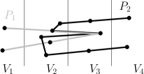
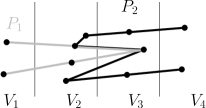
Figure 3: An infeasible pair of an 1-cap $P_{1}$ and a 4-cup $P_{2}$ (top); and a feasible pair of an 1-cap $P_{1}$ and a 4-cup $P_{2}$ (bottom).

Definition of an $i$-cap and $i$-cup.

A path $P$ in $G$ is an $i$-cap and $j$-cup if for the end vertices $u,v$ of $P$ and all $w\not=u,v$ of $P$ we have $\min(P)=\gamma(u)=\gamma(v)=i\not=\gamma(w)$ and $\max(P)=\gamma(u)=\gamma(v)=j\not=\gamma(w)$, respectively, (see Figure 2). A pair of an $i$-cap $P_{1}$ and $j$-cup $P_{2}$ is interleaving if (i) $\min(P_{1})<\min(P_{2})\leq\max(P_{1})<\max(P_{2})$; and (ii) $P_{1}$ and $P_{2}$ intersect in a path (or a single vertex). An interleaving pair of an oriented $i$-cap $P_{1}$ and $j$-cup $P_{2}$ is infeasible, if $i_{\mathcal{E}}(P_{1},P_{2})\not=0$, and feasible, otherwise (see Figure 3). Thus, feasibility does not depend on the orientation. Note that $i_{\mathcal{E}}(P_{1},P_{2})$ can be either $0,1$ or $-1$. Throughout the paper by an infeasible and feasible pair of paths we mean an infeasible and feasible, respectively, interleaving pair of an $i$-cap and $j$-cup.

Observation 2.1.

In $\mathcal{E}$ there does not exist an infeasible interleaving pair $P_{1}$ and $P_{2}$ of an $i$-cap and $j$-cup, $i+1<j$.

As a special case of Observation 2.1 we obtain the following.

Observation 2.2.

The incoming and outgoing edges do not alternate at any vertex $v$ of $\overrightarrow{G}$ (defined in Section 2.1) in the rotation given by $\mathcal{E}$, i.e., the incoming and outgoing edges incident to $v$ form two disjoint intervals in the rotation at $v$.

We say that a vertex $v\in V(G)$ is trapped in the interior of a cycle $C$ if in $\mathcal{E}$ the vertex $v$ is in the interior of $C$ and we have $\min(C)>\gamma(v)$ or $\gamma(v)>\max(C)$, where $\max(C)$ and $\min(C)$, respectively, denotes the maximal and minimal label of a vertex of $C$. A vertex $v$ is trapped if it is trapped in the interior of a cycle.

Observation 2.3.

In $\mathcal{E}$ there does not exist a trapped vertex.

2.4 Proof of Lemma 1.1

Proof.

W.l.o.g. we assume that $G$ is connected. By [13, Lemma 2] we deform the given $x$-bounded embedding into an $x$-bounded drawing in which every pair of edges cross an even number of times. In the obtained drawing, we contract every connected component of $G$ induced by vertices with the same $\gamma$ value to a point thereby possibly obtaining loops at vertices. Let $(G^{\prime},\gamma^{\prime})$ denote the resulting pair. Note that in the drawing of $G^{\prime}$ every pair of edges still cross an even number of times. Hence, in $G^{\prime}$ the loops can be redrawn in the close vicinity of their vertices thereby making them crossing free without changing the rotation system. See the proof of Theorem 1 in [15] for a more formal treatment of the previous argument. By using the corresponding variant of the weak Hanani–Tutte theorem [13, Theorem 1] we obtain an $x$-bounded embedding of $(G^{\prime},\gamma^{\prime})$ in which $x(e)$ of every non-loop edge $e\in E$ is injective without changing the rotation at vertices. Indeed, the $x$-monotonicity follows directly from the proof. The contracted components $C$ can be recovered as follows. We embed $C$ represented in $G^{\prime}$ by a vertex $v$ in a close vicinity of $v$ by Tutte’s barycenter algorithm [35]. To this end we first sub-divide edges incident to $v$ and un-contract $C$ (which is possible since we did not change the rotations, and thus, the loops at $v$ are still edge-crossing free). Let $C^{\prime}$ denote the union of $C$ with the edges leaving $C$. Due to sub-divisions of the edges incident to $v$ all the edges leaving $C$ have degree one. Let $v_{1},\ldots,v_{k}$ denote those degree-one (in $C^{\prime}$) vertices. Note that $v_{i}$’s have degree two in $G^{\prime}$. We augment the obtained embedding of $C^{\prime}$ into an internally triangulated planar graph $C^{\prime\prime}$ having the outer face bounded by the cycle $v_{1},\ldots,v_{k}$. In the embedding $\mathcal{D}$ obtained by the variant of the weak Hanani–Tutte theorem [13, Theorem 1] we replace a small disc neighborhood $D_{v}$ of $v$ by the straight-line embedding of $C^{\prime\prime}$ obtained by an application of Tutte’s barycenter algorithm. We assume that $v_{i}$’s are drawn on the boundary of $D_{v}$ in $\mathcal{D}$. In the barycentric embedding of $C^{\prime\prime}$ the vertices $v_{1},\ldots,v_{k}$ are prescribed to lie on the boundary of $D_{v}$ as in $\mathcal{D}$. By recovering contracted components in $\mathcal{D}$ one by one as above the claim follows.   

3 Characterization of isotopy classes containing $x$-bounded embeddings

In this section we prove our characterization of isotopy classes $\mathcal{E}$ of $G$ containing an $x$-bounded embedding w.r.t. $(G,\gamma)$ by reducing a general instance of to a normalized one.

Theorem 3.1.

The isotopy class $\mathcal{E}$ of $G$ contains an $x$-bounded embedding w.r.t. $(G,\gamma)$ if and only if $\mathcal{E}$ does not contain an infeasible interleaving pair of paths, or a trapped vertex.

Before we turn to the proof of Theorem 3.1 we discuss its relation to Theorem 1.2. The condition that $\mathcal{E}$ does not contain a trapped vertex is an equivalent reformulation of the condition that $i_{\mathcal{E}}(D,v)=0$, where $D$ is a union of faces with a disc as a support, if $\gamma(\partial(D)=C)\cap\gamma(v)=\emptyset$. Regarding the condition for pairs of paths, Theorem 3.1 seems to be stronger than Theorem 1.2 due to a more restricted condition on pairs of paths we consider. However, the strengthening is not significant, since it can be easily shown that forbidding an infeasible interleaving pair of paths and trapped vertices renders the hypothesis of the “if” part of Theorem 1.2 satisfied, and thus, we get its equivalence with Theorem 3.1.

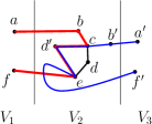
Figure 4: Replacing the portion of $P_{1}^{\prime}=abcdef$ with the portion of $P_{2}^{\prime}=a^{\prime}b^{\prime}cd^{\prime}ef^{\prime}$ on the cycle $C=cded^{\prime}$.

Indeed, if a pair of intersecting paths $P_{1}$ and $P_{2}$ satisfies $\gamma(P_{1})\cap\gamma(\partial P_{2})=\emptyset$ and $\gamma(\partial P_{1})\cap\gamma(P_{2})=\emptyset$, there exist sub-paths $P_{1}^{\prime}$ of $P_{1}$ and $P_{2}^{\prime}$ of $P_{2}$ such that $i_{\mathcal{E}}(P_{1},P_{2})=i_{\mathcal{E}}(P_{1}^{\prime},P_{2}^{\prime})$ that either form an interleaving pair or do not form an interleaving pair only because they do not intersect in a path. In the latter, no end vertex of $P_{1}$ or $P_{2}$ is contained in the interior of a cycle in $P_{1}^{\prime}\cup P_{2}^{\prime}$ due to the non-existence of trapped vertices. Let $W_{2}$ be a walk obtained from $P_{2}^{\prime}$ by replacing its portion on a cycle $C$ contained in $P_{1}^{\prime}\cup P_{2}^{\prime}$, such that $P_{1}^{\prime}\cap C$ is a path, with the portion of $P_{1}^{\prime}$ for every such cycle (see Figure 4). Let $P_{2}^{\prime\prime}$ denote the path in $W_{2}$ connecting its end vertices. We have $i_{\mathcal{E}}(P_{1},P_{2})=i_{\mathcal{E}}(P_{1}^{\prime},P_{2}^{\prime\prime})$, and $P_{1}^{\prime}$ and $P_{2}^{\prime\prime}$ form an interleaving pair. Hence, we just proved the following.

Lemma 3.2.

Given that $(G,\gamma)$ is free of trapped vertices, if a pair of intersecting paths $P_{1}$ and $P_{2}$ in $\mathcal{E}$ satisfies $\gamma(P_{1})\cap\gamma(\partial P_{2})=\emptyset$ and $\gamma(\partial P_{1})\cap\gamma(P_{2})=\emptyset$, there exist sub-paths $P_{1}^{\prime}$ of $P_{1}$ and $P_{2}^{\prime}$ of $P_{2}$ such that $i_{\mathcal{E}}(P_{1},P_{2})=i_{\mathcal{E}}(P_{1}^{\prime},P_{2}^{\prime\prime})$, where $P_{2}^{\prime\prime}\subset P_{1}^{\prime}\cup P_{2}^{\prime}$ is constructed as above, forming an interleaving pair.

proof of Theorem 3.1.

The proof is inspired by the work of Minc [22] and M. Skopenkov [33]. By sub-dividing edges of $G$ we (tacitly) assume $|\gamma(u)-\gamma(v)|\leq 1$, for every edge $uv\in E(G)$. We proceed by the induction on the number of clusters $c$ and
$\lambda:=\lambda(G,\gamma)=\sum_{V_{i}}\sum_{C_{j}}(|V(C_{j})|-1)$, where the inner sum is over the connected components $C_{j}$ induced by $V_{i}$, in this order.

Suppose that $\lambda>0$. It follows that we have an edge $e$ in $E(G)$ between two vertices $u,v$ with the same $\gamma$ value. We contract $e$ into a vertex $w$ in an embedding of $G$ from the given isotopy class thereby decreasing $\lambda$. We put $\gamma^{\prime}(w):=\gamma(u)$ and $\gamma^{\prime}(z):=\gamma(z)$ for every other vertex of $G$. Let $(G^{\prime},\gamma)$ denote the obtained pair. The resulting drawing is still an embedding but we could introduced a loop at $w$ by the contraction. However, we did not introduce a trapped vertex or an infeasible interleaving pair of paths. In particular, if there exists a loop incident to $w$ it contains only vertices with the same $\gamma$ value as $w$. We delete such loops together with its interior. We apply the induction hypothesis on the obtained pair $(G^{\prime\prime},\gamma^{\prime\prime})$ with the isotopy class of its obtained embedding thereby obtaining an $x$-bounded embedding of $(G^{\prime\prime},\gamma^{\prime\prime})$. In the $x$-bounded embedding of $G^{\prime}$ we re-introduce deleted loops with their interiors at the same position in the rotation at $w$. Then by splitting $w$ into $e$ we obtain a desired $x$-bounded embedding of $(G,\gamma)$.

Hence, suppose that $\lambda=0$. Let $v_{i}\in V_{i}$, $i=0,\ldots,c-1$, such that $v_{i}$ is joined by an edge with a vertex $u_{i+1}\in V_{i+1}$ and a vertex $w_{i-1}\in V_{i-1}$. We apply a vertex split to every such $v_{i}$ thereby obtaining a pair of new vertices $v_{i}^{\prime}$ and $v_{i}^{\prime\prime}$ joined by an edge such that $\gamma(v_{i}^{\prime})=\gamma(v_{i}^{\prime\prime}):=\gamma(v_{i})=i$. The vertex $v_{i}^{\prime}$ is joined by an edge with neighbors of $v_{i}$ in $V_{i-1}$ and $v_{i}^{\prime\prime}$ is joined by an edge with neighbors of $v_{i}$ in $V_{i+1}$. Let $(G^{\prime},\gamma^{\prime})$ denote the obtained pair. We assume that the rotation system of $G^{\prime}$ is such that by contracting the edges introduced by the splits we obtain an embedding in the given isotopy class of $G^{\prime}$. Since we have no infeasible interleaving pair in $(G,\gamma)$ this is possible. Let $G_{i}$, for $i=1,\ldots,c-1$, denote the sub-graph of $G^{\prime}$ induced by the edges in $G^{\prime}$ between $V_{i}^{\prime}$ and $V_{i-1}^{\prime}$, i.e, the sets of vertices with $\gamma^{\prime}$ value $i$ and $i-1$. Note that $G_{i}$ is an induced sub-graph of $G^{\prime}$. Let $(G^{\prime},\gamma^{\prime\prime})$ be such that the image of $\gamma^{\prime\prime}$ has $c-1$ different values and $\gamma^{\prime\prime}(V(G_{1}))=1,\ldots,\gamma^{\prime\prime}(V(G_{c-1}))=c-1$. We show that $(G^{\prime},\gamma^{\prime\prime})$ contains neither an interleaving pair of paths nor a trapped vertex.

For the sake of contradiction, suppose that $(G^{\prime},\gamma^{\prime\prime})$ contains an infeasible interleaving pair of paths, an $i$-cap $P_{1}^{\prime}$ and $j$-cup $P_{2}^{\prime}$. Note that we can assume that $P_{1}^{\prime}$ ends in a vertex from $V(G_{i})\cap V_{i-1}^{\prime}$ and $P_{2}^{\prime}$ ends in a vertex from $V(G_{j})\cap V_{j}^{\prime}$. Then we see that $P_{1}^{\prime}$ and $P_{2}^{\prime}$ yield an infeasible interleaving pair in $(G,\gamma)$ (contradiction). Similarly, we can argue about trapped vertices. Hence, by the induction hypothesis $(G^{\prime},\gamma^{\prime\prime})$ admits an $x$-bounded embedding. Let $\mathcal{E}$ denote the corresponding $x$-bounded embedding.

Note that $G_{i}$, for $i=1,\ldots,c-1$, is a bipartite graph with partitions $V_{i-1}^{\prime}\cap V(G_{i})$ and $V_{i}^{\prime}\cap V(G_{i})$, both inducing an independent set. We showed that every c-graph with two-clusters, both inducing an independent set, is c-planar [15]. Moreover, an arbitrary isotopy class can be chosen for the corresponding embedding. Note that the restriction of the $x$-bounded embedding of $(G^{\prime},\gamma^{\prime\prime})$ to $G_{i}$ has vertices joining $G_{i}$ with $G^{\prime}\setminus G_{i}$ on the outer face $f_{i}$ of $G^{\prime}$, and in the facial walk of $f_{i}$ wedges containing the edges between $V(G_{i})$ and $G_{i+1}$ do not alternate with wedges containing the edges between $V(G_{i})$ and $G_{i-2}$. For otherwise we would obtain an infeasible interleaving pair in $(G^{\prime},\gamma^{\prime\prime})$. Hence, such clustered embeddings of $G_{i}$, for $i=1,\ldots,c-1$, can be put next to each other and connected by edges so as to obtain an embedding of $G^{\prime}$ in the given isotopy class. It follows that if we put $\gamma^{\prime\prime\prime}(V_{i-1}\cap V(G_{i})):=2i-2$ and $\gamma^{\prime\prime\prime}(V_{i}\cap V(G_{i})):=2i-1$, the obtained embedding of $G^{\prime}$ can be deformed to obtain an $x$-bounded embedding of $(G^{\prime},\gamma^{\prime\prime\prime})$. The corresponding $x$-bounded embedding of $(G^{\prime},\gamma^{\prime\prime\prime})$ is turned into an $x$-bounded embedding of $(G,\gamma)$ by edge contractions and re-scaling $\gamma^{\prime\prime\prime}$, and this concludes the proof.   

4 Corollaries of the characterization

4.1 The variant of the weak Hanani–Tutte theorem for $x$-bounded drawings

In this section we prove the weak Hanani-Tutte theorem for $x$-bounded drawings, Theorem 1.3.

Given a drawing of a graph $G$ where every pair of edges cross an even number of times, by the weak Hanani-Tutte theorem [9, 24, 27], we can obtain an embedding of $G$ with the same rotation system, and hence, the facial structure of an embedding of $G$ is already present in an even drawing. This allows us to speak about faces in an even drawing of $G$. Hence, a face in an even drawing of $G$ is the walk bounding the corresponding face in the embedding of $G$ with the same rotation system.

A face $f$ in an even drawing corresponds to a closed (possibly self-crossing) curve $C_{f}$ traversing the edges of the defining walk of $f$ in a close vicinity of its edges without crossing an edge that is being traversed, i.e, $C_{f}$ never switches to the other side of an edge it follows. An inner face in an even drawing of $G$ is a face for which all the vertices of $G$ except those incident to $f$ are outside of $C_{f}$. Similarly, an outer face in an even drawing of $G$ is a face such that all the vertices of $G$ except those incident to $f$ are inside of $C_{f}$. Note that by the weak Hanani–Tutte theorem every face is either an inner face or an outer face. Unlike in the case of an embedding (in the plane), in an even drawing the outer face might not be unique. Nevertheless, an outer face always exists in an even drawing of a graph in the plane.

Lemma 4.1.

Every even drawing of a connected graph $G$ in the plane has an odd number of outer faces.

Proof.

Refer to Figure 5. By successively contracting every edge in an even drawing of $G$ we obtain a vertex $v$ with a bouquet of loops, see e.g., the proof of  [27, Theorem 1.1]. Let $\mathcal{D}$ be the obtained drawing whose underlying abstract graph is not simple unless it is edgeless. Let us treat $\mathcal{D}$ as an even drawing. Thus, we obtain the facial structure in $\mathcal{D}$ by traversing walks consisting of loops at $v$. Every loop $l$ at $v$ corresponds to a cyclic interval in the rotation at $v$ containing the end pieces of edges that are in a close neighborhood at $v$ contained inside $l$. By treating every walk in $\mathcal{D}$ as a walk along cyclic intervals of the loops it traverses we define the winding number of a face in $\mathcal{D}$ as the number of times we walk around $v$ when traversing the intervals of its walk. The winding number can be positive or negative depending on the sense of the traversal.

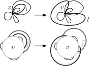
Figure 5: A bouquet of loops at $v$ and its modification after we pull a loop $l$ over $v$ (top). The cyclic intervals corresponding to the loops in the rotation at $v$ before and after we pull $l$ over $v$ (bottom).

Note that the outer faces in $\mathcal{D}$ are those faces $f$ whose corresponding walks wind around $v$ an odd number of times. This follows because whenever we visit $v$ during a walk of $f$ winding an odd number of times around $v$ the corresponding position in the rotation at $v$ is contained inside of an even number of loops of the walk, and hence outside of $C_{f}$.

By pulling a loop $l$ over $v$ we flip the cyclic interval in its rotation that corresponds to the inside of $l$. It follows that we change the winding number of both facial walks that $l$ participates in by one. Hence, we do not change the parity of the total number of outer faces in $\mathcal{D}$. Since a crossing free drawing of $G$ has an odd number of outer faces the lemma follows.   

Given an even $x$-bounded drawing of $(G,\gamma)$ we can associate it with the isotopy class $\mathcal{E}$ of a corresponding embedding of $G$. Note that by the connectivity of $G$ the interval spanned by the $\gamma$ values of the vertices incident to the outer face $f$ in $\mathcal{E}$, which can be chosen by Lemma 4.1, span all the values $\gamma$. By Theorem 3.1 it is enough to prove that $\mathcal{E}$ does not contain an infeasible pair of paths or a vertex trapped in the interior of a cycle. However, due to evenness of the given drawing of $G$ both of these forbidden substructures would introduce a pair of cycles crossing an odd number of times (contradiction). In order to rule out the existence of a trapped vertex we use the fact that the boundary of the outer face $f$ spans all the values of $\gamma$. If a vertex $v$ is trapped in the interior of a cycle $C$ then by the connectedness of $G$ we can join $C$ with $v$ by a path $P$ of $G$. By the evenness of the drawing it follows that the end piece of $P$ at $C$ in our drawing start outside of $C$. On the other hand, a path connecting $C$ with any vertex on the outer face $f$ must also start at $C$ outside of $C$, since the boundary of $f$ spans all the values of $\gamma$. Thus, $v$ cannot be trapped, since the rotation system from the even drawing is preserved in the embedding.

4.2 Strip clustered graphs and c-planarity

A clustered graph is an ordered pair $(G,T)$, where $G$ is a graph, and $T=\{V_{i}|i=1,\ldots,k\}$ is a partition of the vertex set of $G$ into $k$ parts. We call the sets $V_{i}$ clusters. A drawing of a clustered graph $(G,T)$ is clustered if vertices in $V_{i}$ are drawn inside a topological disc $D_{i}$ for each $i$ such that $D_{i}\cap D_{j}=\emptyset$ and every edge of $G$ intersects the boundary of every disc $D_{i}$ at most once. We use the term “cluster $V_{i}$” also when referring to the topological disc $D_{i}$ containing the vertices in $V_{i}$. A clustered graph $(G,T)$ is clustered planar (or briefly c-planar) if $(G,T)$ has a clustered embedding.

A strip clustered graph is a concept introduced recently by Angelini et al. [1] For convenience we slightly alter their definition and define “strip clustered graphs” as “proper” instances of “strip planarity” in [1]. In the present paper we are primarily concerned with the following subclass of clustered graphs. A clustered graph $(G,T)$ is strip clustered if $G=\left(V_{1}\cup\ldots\cup V_{k},E\subseteq\bigcup_{i}{V_{i}\cup V_{i+1}\choose 2}\right)$, i.e., the edges in $G$ are either contained inside a part or join vertices in two consecutive parts. A drawing of a strip clustered graph $(G,T)$ in the plane is strip clustered if $i<x(v_{i})<i+1$ for all $v_{i}\in V_{i}$, and every line of the form $x=i$, $i\in\mathbb{N}$, intersects every edge at most once. Thus, strip clustered drawings constitute a restricted class of clustered drawings. We use the term “cluster $V_{i}$” also when referring to the vertical strip containing the vertices in $V_{i}$. A strip clustered graph $(G,T)$ is strip planar if $(G,T)$ has a strip clustered embedding in the plane. Note that if we define $(G,\gamma)$, so that $\gamma(v)=i$ for $v\in V_{i}$, a strip clustered drawing is $x$-bounded. Thus, Theorem 1.6 implies an efficient algorithm for strip planarity testing.

Lemma 4.2.

The problem of strip planarity testing is reducible in linear time to the problem of c-planarity testing in the case of flat clustered graphs with three clusters.

Proof.

Given an instance of $(G,T)$ of strip clustered graph we construct a clustered graph $(G,T^{\prime})$ with three clusters $V_{0}^{\prime},V_{1}^{\prime}$ and $V_{2}^{\prime}$ as follows. We put $T^{\prime}=\{V_{j}^{\prime}|\ V_{j}^{\prime}=\bigcup_{i;\ i\mod 3=j}V_{i}\}$. Note that without loss of generality we can assume that in a drawing of $(G,T^{\prime})$ the clusters are drawn as regions bounded by a pair of rays emanating from the origin. By the inverse of a projective transformation taking the origin to the vertical infinity we can also assume that the same is true for a drawing of $(G,T)$. Notice that such clustered embedding of $(G,T)$ can be continuously deformed by a rotational transformation of the form $(\phi,r)\rightarrow(k\phi,c\phi\cdot r)$ for appropriately chosen $k,c>1$, which is expressed in polar coordinates, so that we obtain a clustered embedding of $(G,T^{\prime})$. We remark that $(x,y)$ in Cartesian coordinates corresponds to $(\phi,\sqrt{x^{2}+y^{2}})$ such that $\sin\phi=\frac{y}{\sqrt{x^{2}+y^{2}}}$ and $\cos\phi=\frac{x}{\sqrt{x^{2}+y^{2}}}$ in polar coordinates. On the other hand, it is not hard to see that if $(G,T^{\prime})$ is c-planar then there exists a clustered embedding of $(G,T^{\prime})$ with the following property. For each $i=0,1,2$ and $j$ the vertices of $V_{i}^{\prime}$ belonging to $V_{j}$ and the parts of their adjacent edges in the region representing $V_{j}^{\prime}$ belong to a topological disc $D_{j}$ such that $D_{j}\cap D_{j^{\prime}}=\emptyset$ for $j\not=j^{\prime}$ fully contained in this region. To this end we proceed as follows. Let $E_{i}=E[V_{i-1},V_{i}]$ denote the edges in $G$ between $V_{i-1}$ and $V_{i}$. Let $r_{i}$ denote the ray emanating from the origin that separates $V_{i-1}^{\prime}$ from $V_{i}^{\prime}$. Given a clustered drawing of $(G,T^{\prime})$, $p_{e}(\mathcal{E})$, for $e\in E_{i}$, is the intersection point of $e$ with the ray $r_{i\mod 3}$. Let $p$ denote the origin. Let $|pq|$ for a pair of points in the plane denote the Euclidean distance between $p$ and $q$. Recall that $G$ has clusters $V_{1},\ldots,V_{k}$. We obtain a desired embedding of $(G,T^{\prime})$ inductively as $\mathcal{E}_{k}$ starting with $\mathcal{E}_{4}$. For $\mathcal{E}_{i}=(G,T^{\prime})$, $i=5,\ldots,k$, we maintain the following invariant. For each $j,\ 5\leq j\leq i$, we have

$$\max_{e\in E[V_{j-4},V_{j-3}]}|pp_{e}|<\min_{e\in E[V_{j-1},V_{j}]}|pp_{e}|\ \ (*).$$

Let $\mathcal{E}$ denote a clustered embedding of $(G,T^{\prime})$. We start with a clustered embedding of $\mathcal{E}_{4}$ of $(G[V_{1}\cup V_{2}\cup V_{3}\cup V_{4}],T^{\prime})$ inherited from $\mathcal{E}$. In the $i^{\mathrm{th}}$ step of the induction we extend $\mathcal{E}_{i-1}$ of $(G[V_{1}\cup V_{2}\ldots\cup V_{i-1}],T^{\prime})$ inside the wedge corresponding to $V_{i-1\mod 3}^{\prime}$ and $V_{i\mod 3}^{\prime}$ thereby obtaining an embedding $\mathcal{E}_{i}$ of $(G[V_{1}\cup V_{2}\ldots\cup V_{i}],T^{\prime})$ so that the resulting embedding $\mathcal{E}_{i}$ is still clustered, and $(*)$ is satisfied. Since by induction hypothesis we have $\max_{e\in E[V_{i-3j-2},V_{i-3j-1}]}|pp_{e}|<\min_{e\in E[V_{i-2},V_{i-1}]}|pp_{e}|$, for all possible $j$, in $\mathcal{E}_{i-1}$ we have $G[V_{i-1}]$ drawn in the outer face of $G[V_{1}\cup\ldots\cup V_{i-2}]$. Thus, we can extend the embedding of $\mathcal{E}_{i-1}$ into $\mathcal{E}_{i}$ in which all the edges of $E_{i}$ cross $r_{i\mod 3}$ in the same order as in $\mathcal{E}$ while maintaining the invariant $(*)$ and the rotation system inherited from $\mathcal{E}$. The obtained embedding $\mathcal{E}_{k}$ of $(G,T^{\prime})$ can be easily transformed into a strip clustered embedding.

Thus, $(G,T)$ is strip planar if and only if $(G,T^{\prime})$ is c-planar.   

If $G$ is a tree also the converse of Lemma 4.2 is true. In other words, given an instance of clustered tree $(G,T)$ with three clusters $V_{0},V_{1}$ and $V_{2}$ we can easily construct a strip clustered tree $(G,T^{\prime})$ with the same underlying abstract graph such that $(G,T^{\prime})$ is strip planar if and only if $(G,T)$ is c-planar. Indeed, the desired equivalent instance is obtained by partitioning the vertex set of $G$ into clusters thereby obtaining $(G,T^{\prime}=\{V_{i}^{\prime}|\ i\in I\subset\mathbb{N}\})$ as follows. In the base case, pick an arbitrary vertex $v$ from a non-empty cluster $V_{i}$ of $G$ into $V_{i}^{\prime}$, and no vertex is processed.

In the inductive step we pick an unprocessed vertex $u$ that was already put into a set $V_{j}^{\prime}$ for some $j$. We put neighbors of $u$ in $V_{j\mod 3}$ into $V_{j}^{\prime}$, neighbors in $V_{j+1\mod 3}$ into $V_{j+1}^{\prime}$, and neighbors of $v$ in $V_{j-1\mod 3}$ into $V_{j-1}^{\prime}$. Then we mark $u$ as processed. Since $G$ is a tree, the partition $T^{\prime}$ is well defined. Now, the argument of Lemma 4.2 gives us the following.

Lemma 4.3.

The problem of c-planarity testing in the case of flat clustered graphs with three clusters is reducible in linear time to the strip planarity testing if the underlying abstract graph is a tree.

4.3 The variant of the Hanani-Tutte theorem for $x$-bounded drawings and 3-connected graphs

In this section we prove the Hanani-Tutte theorem for $x$-bounded drawings if the underlying abstract graph is three connected, Theorem 1.5.

First, we prove a lemma that allows us to get rid of odd crossing pairs by doing only local redrawings and vertex splits. A drawing of a graph $G$ is obtained from the given drawing of $G$ by redrawing edges locally at vertices if the resulting drawing of $G$ differs from the given one only in small pairwise disjoint neighborhoods of vertices not containing any other vertex. The proof of the following lemma is inspired by the proof of [27, Theorem 3.1].

Lemma 4.4.

Let $G$ denote a subdivision of a vertex three-connected graph drawn in the plane so that every pair of non-adjacent edges cross an even number of times. We can turn the drawing of $G$ into an even drawing by a finite sequence of local redrawings of edges at vertices and vertex splits.

Proof.

We process cycles in $G$ containing an edge crossed by one of its adjacent edges an odd number of times one by one until no such cycle exists. Let $C$ denote a cycle of $G$. By local redrawings at the vertices of $C$ we obtain a drawing of $G$, where every edge of $C$ crosses every other edge an even number of times. Let $v$ denote a vertex of $C$.

First, suppose that every edge incident to $v$ and starting inside of $C$ crosses every edge incident to $v$ and starting outside of $C$ an even number of times. In this case we perform at most two subsequent vertex splits. If there exists at least two edges starting at $v$ inside (outside) of $C$, we split $v$ into two vertices $v^{\prime}$ and $v^{\prime\prime}$ joined by a very short crossing free edge so that $v^{\prime}$ is incident to the neighbors of $v$ formerly joined with $v$ by edges starting inside (outside) of $C$, and $v^{\prime\prime}$ is incident to the rest of the neighbors of $v$. Thus, $v^{\prime\prime}$ replaces $v$ on $C$. Notice that by splitting we maintain the property of the drawing to be independently even, and the property of our graph to be three-connected. Moreover, all the edges incident to the resulting vertex $v^{\prime\prime}$ of degree three or four cross one another an even number of times. Hence, no edge of $C$ will ever be crossed by another edge an odd number of times, after we apply appropriate vertex splits at every vertex of $C$.

Second, we show that there does not exist a vertex $v$ incident to $C$ so that an edge $vu$ starting inside of $C$ crosses an edge $vw$ starting outside of $C$ an odd number of times. Since $G$ is a subdivision of a vertex three-connected graph, there exist two distinct vertices $u^{\prime}$ and $w^{\prime}$ of $C$ different from $v$ such that $u^{\prime}$ and $w^{\prime}$, respectively, is connected with $u$ and $w$ by a path internally disjoint from $C$. Let $uP_{1}u^{\prime}$ and $wP_{2}w^{\prime}$, respectively, denote this path. Note that $u$ can coincide with $u^{\prime}$ and $w$ can coincide with $w^{\prime}$. Let $vP_{3}u^{\prime}$ denote the path contained in $C$ no passing through $w^{\prime}$. Let $C^{\prime}$ denote the cycle obtained by concatenation of $P_{1}$, $P_{3}$, and $vu$. Let $C^{\prime\prime}$ denote the cycle obtained by concatenating $P_{2}$ and the portion of $C$ between $w^{\prime}$ and $v$ not containing $u^{\prime}$. Since $vw$ and $vu$ cross an odd number of times and all the other pairs of edges $e\in E(C^{\prime})$ and $f\in E(C^{\prime\prime})$ cross an even number of times, the edges of $C^{\prime}$ and $C^{\prime\prime}$ cross an odd number of times. It follows that their corresponding curves cross an odd number of times (contradiction).

Notice that by vertex splits we decrease the value of the function $\sum_{v\in V(G)}deg^{3}(v)$ whose value is always non-negative. Hence, after a finite number of vertex splits we turn $G$ into an even drawing of a new graph $G^{\prime}$.   

We turn to the actual proof of Theorem 1.5.

We apply Lemma 4.4 to $(G,\gamma)$ thereby obtaining $(G^{\prime},\gamma^{\prime})$, where each vertex obtained by a vertex split, has the $\gamma^{\prime}$ value as its parental vertex. By applying Theorem 1.3 to $(G^{\prime},\gamma^{\prime})$ we obtain a clustered embedding of $(G^{\prime},\gamma^{\prime})$. Finally, we contract the pairs of vertices obtained by vertex splits in order to obtain an $x$-bounded embedding of $(G,\gamma)$.

5 Trees

In this section we give an algorithm proving Theorem 1.6.

In order to make the present section easier do digest, as a warm-up we give an algorithm in the case, when $G$ is a subdivided star. Then we show that a slightly more involved algorithm based on the same idea also works for general trees. Throughout the present section we (tacitly) assume the following

$$(*)\ \ \ |\gamma(u)-\gamma(v)|\leq 1$$

for every edge $uv\in E(G)$. Thus, we can think of proving the result for strip clustered graphs, which is how we thought about it originally.

5.1 Subdivided stars

In the sequel $G=(V,E)$ is a subdivided star. Thus, $G$ is a connected graph that contains a special vertex $v$, the center of the star, of an arbitrary degree and all the other vertices in $G$ are either of degree one or two. The assumption $(*)$ can be imposed without loss of generality. Indeed, by subdividing every edge $uv$ by vertices $w$ for which $\gamma(u)<\gamma(w)<\gamma(v)$ we do not change the embeddability.

Recall that $\max(G^{\prime})$ and $\min(G^{\prime})$, respectively, denote the maximal and minimal value of $\gamma(v)$, $v\in V(G^{\prime})$, and that a path $P$ in $G$ is an $i$-cap and $i$-cup, respectively, if for the end vertices $u$ and $v$ of $P$ and all $w\not=u,v$ of $P$ we have $\min(P)=\gamma(u)=\gamma(v)=i\not=\gamma(w)$ and $\max(P)=\gamma(u)=\gamma(v)=i\not=\gamma(w)$.

The following lemma is a direct consequence of our characterization stated in Theorem 3.1.

Lemma 5.1.

Let us fix a rotation at $v$, and thus, an embedding of $G$. Suppose that every interleaving pair of an $i$-cap $P_{1}$ and $j$-cup $P_{2}$ in $G$ containing $v$ in their interiors is feasible in the fixed embedding of $G$. Then $(G,\gamma)$ admits an $x$-bounded embedding and in a corresponding embedding of $(G,T)$ the rotation at $v$ is preserved.

In what follows we show how to use Lemma 5.1 for a polynomial-time $x$-bounded embeddability testing if the underlying abstract graph is a subdivided star. The algorithm is based on testing in polynomial time whether the columns of a 0–1 matrix can be ordered so that, in every row, either the ones or the zeros are consecutive. We, in fact, consider matrices containing $0,1$ and also an ambiguous symbol $*$. A matrix containing 0,1 and $*$ as its elements has the circular-ones property if there exists a permutation of its columns such that in every row, either the ones or the zeros are consecutive among undeleted symbols after we delete all $*$. Then each row in the matrix corresponds to a constraint imposed on the rotation at $v$ by Lemma 5.1 simultaneously for many pairs of paths.

By Lemma 5.1 it is enough to decide if there exists a rotation at $v$ so that every interleaving pair of an $s$-cap $P_{1}$ and $b$-cup $P_{2}$ meeting at $v$ is feasible. Note that if either $P_{1}$ or $P_{2}$ does not contain $v$ in its interior the corresponding pair is feasible. An interleaving pair $P_{1}$ and $P_{2}$ passing through $v$ restricts the set of all rotations at $v$ in an $x$-bounded embedding of $(G,\gamma)$. Namely, if $e_{i}$ and $f_{i}$ are edges incident to $P_{i}$ at $v$ then in an $x$-bounded embedding of $(G,\gamma)$ in the rotation at $v$ the edges $e_{1},f_{1}$ do not alternate with the edges $e_{2},f_{2}$, i.e., $e_{1}$ and $f_{1}$ are consecutive when we restrict the rotation to $e_{1},f_{1},e_{2},f_{2}$. We denote such a restriction by $\{e_{1}f_{1}\}\{e_{2}f_{2}\}$. Given a cyclic order $\mathcal{O}$ of edges incident to $v$, we can interpret $\{e_{1}f_{1}\}\{e_{2}f_{2}\}$ as a Boolean predicate which is “true” if and only if $e_{1},f_{1}$ do not alternate with the edges $e_{2},f_{2}$ in $\mathcal{O}$. Of course, for a given cyclic order we have $\{ab\}\{cd\}$ if and only if $\{cd\}\{ab\}$, and $\{ab\}\{cd\}$ if and only if $\{ba\}\{cd\}$. Then our task is to decide in polynomial time if the rotation at $v$ can be chosen so that the predicates $\{e_{1}f_{1}\}\{e_{2}f_{2}\}$ of all the interleaving pairs $P_{1}$ and $P_{2}$ are “true”. The problem of finding a cyclic ordering satisfying a given set of Boolean predicates of the form $\{e_{1}f_{1}\}\{e_{2}f_{2}\}$ is NP-complete in general, since the problem of total ordering [23] can be easily reduced to it in polynomial time. However, in our case the instances satisfy the following structural properties making the problem tractable (as we see later).

Observation 5.2.

If $\{ab\}\{cd\}$ is false and $\{ab\}\{de\}$ (is true) then $\{ab\}\{ce\}$ is false.

The restriction on rotations at $v$ by the pair of an $s$-cap $P_{1}$ and $b$-cup $P_{2}$ is witnessed by an ordered pair $(s,b)$, where $s<b$. We treat such pair as an interval in $\mathbb{N}$.
Let $I=\{(s,b)|\ (s,b)\mathrm{\ witness\ a\ restriction\ on\ rotations\ at}\ v\mathrm{\ by\ an\ interleaving\ pair\ of\ paths}\}$.

Observation 5.3.

If an $s$-cap $P$ contains $v$ then $P$ contains an $s^{\prime}$-cap $P^{\prime}$ containing $v$ as a sub-path for every $s^{\prime}$ such that $s<s^{\prime}<\gamma(v)$. Similarly, if a $b$-cup $P$ contains $v$ then $P$ contains a $b^{\prime}$-cup $P^{\prime}$ containing $v$ as a sub-path for every $b^{\prime}$ such that $\gamma(v)<b^{\prime}<b$.

Observation 5.4.

Let $s<s^{\prime}<b<b^{\prime}$, $s,s^{\prime},b,b^{\prime}\in\mathbb{N}$. If the set $I$ contains both $(s,b)$ and $(s^{\prime},b^{\prime})$, it also contains $(s,b^{\prime})$ and $(s^{\prime},b)$.

We would like to reduce the question of determining if we can choose a rotation at $v$ making all the interleaving pairs feasible to the following problem. Let $S=\{e_{1},\ldots,e_{n}\}$ of $n$ elements (corresponding to the edges incident to $v$). Let $\mathcal{S}^{\prime}=\{L_{i}^{\prime},R_{i}^{\prime}|\ i=1,\ldots\}$ of polynomial size in $n$ such that $R_{i}^{\prime},L_{i}^{\prime}\subseteq S$ and $|L_{i}^{\prime}|,|R_{i}^{\prime}|\geq 2,\ L_{i+1}^{\prime}\cup R_{i+1}^{\prime}\subseteq L_{i}^{\prime}\cup R_{i}^{\prime}$. Can we cyclically order $S$ so that both $R_{i}^{\prime}$ and $L_{i}^{\prime}$, for every $R_{i}^{\prime},L_{i}^{\prime}\in\mathcal{S}^{\prime}$, appear consecutively, when restricting the order to $R_{i}^{\prime}\cup L_{i}^{\prime}$? Once we accomplish the reduction, we end up with the problem of testing the circular-ones property on matrices containing $0,1$ and $*$ as elements, where each $*$ has only $*$ symbol underneath. This problem is solvable in polynomial time as we will see later. We construct an instance for this problem which is a matrix $M=(m_{ij})$ as follows. The $i^{\mathrm{th}}$ row of $M$ corresponds to the pair $L_{i}^{\prime}$ and $R_{i}^{\prime}$ and each column corresponds to an element of $S$. For each pair $L_{i}^{\prime},R_{i}^{\prime}$ we have $m_{ij}=0$ if $j\in L_{i}^{\prime}$, $m_{ij}=1$ if $j\in R_{i}^{\prime}$, and $m_{ij}=*$ otherwise. Note that our desired condition on $\mathcal{S}^{\prime}$ implies that in $M$ each $*$ has only $*$ symbols underneath. The equivalence of both problems is obvious.

In order to reduce our problem of deciding if a “good” rotation at $v$ exists, we first linearly order intervals in $I$. Let $(s_{0},b_{0})\in I$ be inclusion-wise minimal interval such that $s_{0}$ is the biggest and similarly let $(s_{1},b_{1})\in I$ be inclusion-wise minimal such that $b_{1}$ is the smallest one. By Observation 5.4 we have $s_{0}=s_{1}$ and $b_{0}=b_{1}$. Thus, let $(s_{0},b_{0})\in I$ be such that $s_{0}$ is the biggest and $b_{0}$ is the smallest one. Inductively we relabel elements in $I$ as follows. Let $(s_{i+1},b_{i+1})\in I$ be such that $s_{i+1}<s_{i}<b_{i}<b_{i+1}$ and subject to that condition $s_{i+1}$ is the biggest and $b_{i+1}$ is the smallest one. By Observation 5.4 all the elements in $I$ can be ordered as follows

$${\bf(s_{0},b_{0})},(s_{0,1},b_{0}),\ldots,(s_{0,i_{0}},b_{0}),(s_{0},b_{0,1}),\ldots(s_{0},b_{0,j_{0}}),{\bf(s_{1},b_{1})},(s_{1,1},b_{1})\ldots,(s_{1},b_{1,j_{1}}),{\bf(s_{2},b_{2})},\ldots$$ (1)

where $s_{k,i+1}<s_{k,i}<s_{k}$ and $b_{k,i+1}>b_{k,i}>b_{k}$. For example, the ordering corresponding to the graph in Figure 6 is $(4,6),(3,6),(2,6),(4,7),(3,7),(2,7)$. Let $E(s,b)$ and $E^{\prime}(s,b)$, respectively, denote the set of all the edges incident to $v$ contained in an $s$-cap and $b$-cup, where $(s,b)\in I$. Thus, $E(s,b)\cup E^{\prime}(s,b)$ contain edges incident to $v$ contained in an interleaving pair that yields a restriction on rotations at $v$ witnessed by $(s,b)$. Note that $E(s,b)\cap E^{\prime}(s,b)=\emptyset$. By Observation 5.3, $E(s_{k,j+1},b_{k})\subseteq E(s_{k,j},b_{k})$ and $E^{\prime}(s_{k},b_{k,j+1})\subseteq E^{\prime}(s_{k},b_{k,j})$. The restrictions witnessed by $(s,b)$ correspond to the following condition. In the rotation at $v$ the edges in $E(s,b)$ follow the edges in $E^{\prime}(s,b)$. Indeed, otherwise we have a four-tuple of edges $e_{1},e_{2},f_{1}$ and $f_{2}$ incident to $v$, such that $e_{1},f_{1}\in P_{1}$ and $e_{2},f_{2}\in P_{2}$, where $P_{1}$ and $P_{2}$ form an interleaving pair of an $s_{i}$-cap and $b_{i}$-cup, violating the restriction $\{e_{1}f_{1}\}\{e_{2}f_{2}\}$ on the rotation at $v$. However, such a four-tuple is not possible in an embedding by Theorem 3.1.

Let $L_{i}=E(s,b)$ and $R_{i}=E^{\prime}(s,b)$, respectively, for $(s,b)\in I$, where $i$ is the index of the position of $(s,b)$ in $(\ref{eqn:order})$. Note that $E(s_{i+1},b_{i+1})\cup E^{\prime}(s_{i+1},b_{i+1})\subseteq E(s_{i},b_{i})\cup E^{\prime}(s_{i},b_{i})$. Our intermediate goal of reducing our problem to the circular-ones property testing would be easy to accomplish if $I$ consisted only of intervals of the form $(s_{i},b_{i})$ defined above. However, in $I$ there might be intervals of the form $(s_{i},b)$, $b\not=b_{i}$, or $(s,b_{i})$, $s\not=s_{i}$. Hence, we cannot just put $L_{i}^{\prime}:=L_{i}$ and $R_{i}^{\prime}:=R_{i}$ for all $i$, since we do necessarily have the condition $L_{i+1}\cup R_{i+1}\subseteq L_{i}\cup R_{i}$ satisfied for all $i$.

Definition of $\mathcal{S}^{\prime}$.

Let $\mathcal{S}=\{L_{i},R_{i}|\ i=1,\ldots\}$. We obtain $\mathcal{S}^{\prime}$ from $\mathcal{S}$ by deleting the least number of elements from $L_{i}$’s and $R_{i}$’s so that $L_{i+1}^{\prime}\cup R_{i+1}^{\prime}\subseteq L_{i}^{\prime}\cup R_{i}^{\prime}$ for every $i$. More formally, $\mathcal{S}^{\prime}$ is defined recursively as $\mathcal{S}_{m}^{\prime}$, where $\mathcal{S}_{1}^{\prime}=\{L_{1}^{\prime},R_{1}^{\prime}|\ L_{1}^{\prime}=L_{1},\ R_{1}^{\prime}=R_{1}\}$ and $\mathcal{S}_{j}^{\prime}=\mathcal{S}_{j-1}\cup\{L_{j}^{\prime},R_{j}^{\prime}|\ L_{j}^{\prime}=L_{j}\cap(L_{j-1}^{\prime}\cup R_{j-1}^{\prime}),R_{j}^{\prime}=R_{j}\cap(L_{j-1}^{\prime}\cup R_{j-1}^{\prime})\}$. Luckily, the following lemma lying at the heart of the proof of our result shows that information contained in $\mathcal{S}^{\prime}$ is all we need.

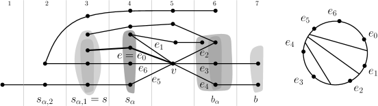
Figure 6: A subdivided star (on the left) with the center $v$, and some restrictions on the set of rotation at $v$ (on the right) corresponding to the intervals $(s_{\alpha},b_{\alpha}),(s_{\alpha,1},b_{\alpha})$ and $(s,b)$. We have $\{e_{0},e_{5},e_{6}\}=E(s_{\alpha,1},b_{\alpha})\subseteq E(s,b)=\{e_{0},e_{2},e_{5},e_{6}\}$ and $\{e_{3},e_{4}\}=E^{\prime}(s,b)\subseteq E^{\prime}(s_{\alpha,1},b_{\alpha})=\{e_{3},e_{4},e_{1},e_{2}\}$. Thus, by removing $e_{0}$ from $E(s,b)$ we obtain the same restrictions on the rotation at $v$.

Lemma 5.5.

We can cyclically order the elements in $S$ so that every pair $L_{i}^{\prime},R_{i}^{\prime}$ in $\mathcal{S}^{\prime}$ gives rise to two disjoint cyclic intervals if and only if $(G,\gamma)$ admits an $x$-bounded embedding.

Proof.

The proof of the lemma is by a double-induction. In the “outer–loop” we induct over $|\mathcal{S}^{\prime}|/2$ while respecting the order of pairs $L_{i},R_{i}$ given by (1). In the “inner–loop” we induct over the size of $S$, where in the base case of the $j^{\mathrm{th}}$ step of the “outer–loop” we have $S_{j,0}=L_{j}^{\prime}\cup R_{j}^{\prime}$. In each ${k}^{\mathrm{th}}$ step of the “inner–loop” we assume by induction hypothesis that a cyclic ordering $\mathcal{O}$ of $S$ satisfies all the restrictions imposed by $\{L_{i},R_{i}|i=1,\ldots,j-1\}$ and $L_{j}\cap S_{j,k-1},R_{j}\cap S_{j,k-1}$. Clearly, once we show that $\mathcal{O}$ satisfies restrictions imposed by $L_{j}\cap S_{j,k},R_{j}\cap S_{j,k}$, where $S_{j,k}=S_{j,k}\cup\{e\}$ and $e\in(L_{j}\cup R_{j})\setminus S_{j,k-1}$ we are done.

Refer to Figure 6. Roughly speaking, by (1) a “problematic” edge $e$ is an initial edge on a path starting at $v$ that never visits a cluster $b_{\alpha}$ after passing through the cluster $s_{\alpha}$ such that $e\in E(s_{\alpha},b_{\alpha})$ (or vice-versa with $E^{\prime}(s_{\alpha},b_{\alpha})$). The edge $e$ is an $(\alpha,\beta)$-lower trim (or $(\alpha,\beta)$-✁) if the lowest index $i$ for which $e\not\in L_{i}^{\prime}\cup R_{i}^{\prime}$ corresponds to $E(s_{\alpha,\beta},b_{\alpha})\cup E^{\prime}(s_{\alpha,\beta},b_{\alpha})$, where $\beta>0$. Analogously, the edge $e$ is an $(\alpha,\beta)$-upper trim (or $(\alpha,\beta)$-✃) if the lowest index $i$ for which $e\not\in L_{i}^{\prime}\cup R_{i}^{\prime}$ corresponds to $E(s_{\alpha},b_{\alpha,\beta})\cup E^{\prime}(s_{\alpha},b_{\alpha,\beta})$, where $\beta>0$. By (1) and symmetry (reversing the order of clusters) we can assume that $e$ is an $(\alpha,\beta)$-✁, and $e\in E(s_{\alpha,\beta-\beta^{\prime}},b_{\alpha})$, for some $\beta^{\prime}>0$, where $s_{\alpha,0}=s_{\alpha}$, and $e\in E(s,b)=L_{j}$, where $s=s_{\alpha,\beta-\beta^{\prime}}$ and $b>b_{\alpha}$, following $E(s_{\alpha,\beta},b_{\alpha})$ in our order. Moreover, we pick $e$ so that $e$ maximizes $i$ for which $e\in L_{i}^{\prime}\cup R_{i}^{\prime}$. We say that $e$ was “trimmed” at the $(i+1)^{\mathrm{th}}$ step.

Figure 7: Three intervals of clusters corresponding to three paths that start at $v$: $P_{e}$ that passes through $e$ and ends in the first vertex in the cluster $s_{\alpha,\beta-1}$, $P_{g^{\prime}}$ that passes through $g^{\prime}$ and ends in a leaf, and $P_{g}$ that ends in the first vertex of the cluster $s^{\prime\prime}$. (An alternative interval for $P_{g}$ is dotted.) Here, $g^{\prime}$ was “trimmed” before $e$.

Thus, $e$ is contained in $E(s,b)$ for some $s,b$ such that $E(s,b),E^{\prime}(s,b)$ follows
$E(s_{\alpha,\beta},b_{\alpha}),E^{\prime}(s_{\alpha,\beta},b_{\alpha})$ in our order. However, it must be that

$$E(s_{\alpha,\beta-\beta^{\prime}}=s,b_{\alpha})\subseteq E(s,b)\ \mathrm{and}\ E^{\prime}(s,b)\subseteq E^{\prime}(s_{\alpha,\beta-\beta^{\prime}}=s,b_{\alpha}),$$ (2)

where the first relation follows directly from the fact $b>b_{\alpha}$ and the second relation is a direct consequence of Observation 5.3. In what follows we show that (2) implies that $\mathcal{O}$ satisfies all the required restrictions involving $e$. We consider an arbitrary four-tuples of edges $e_{1}^{\prime},e_{2}^{\prime},e_{3}^{\prime}\in S_{j,k-1}$ that together with $e$ gives rise to a restriction $\{e_{1}^{\prime}e_{2}^{\prime}\}\{e_{3}^{\prime}e\}$ on $\mathcal{O}$ witnessed by $(s,b)$. The incriminating four-tuple must also contain an element from $E(s,b)\setminus E(s,b_{\alpha})$, let us denote it by $f=e_{3}^{\prime}$. Indeed, otherwise by (2) the restriction is witnessed by $(s,b_{\alpha})$ and we are done by induction hypothesis. Then $e_{1}^{\prime},e_{2}^{\prime}\in E^{\prime}(s,b)$. For the sake of contradiction we suppose that the order $\mathcal{O}$ violates the restriction $\{e_{1}^{\prime}e_{2}^{\prime}\}\{ef\}$. Let $g\in L_{i^{\prime}}^{\prime}\subseteq E(s_{\alpha,\beta},b_{\alpha})$, for some $i^{\prime}$. Note that $g$ exists (see Figure 7) for if an edge $g^{\prime}\in E(s_{\alpha,\beta},b_{\alpha})$ is not in $L_{i^{\prime}}^{\prime}$ it means that $g^{\prime}$ was “trimmed” before $e$ and we can put $g$ to be an arbitrary element from $E(s^{\prime\prime},b^{\prime\prime})$ minimizing $s^{\prime\prime}$ appearing before $E(s_{\alpha},b_{\alpha})$ in our order.

Here, the reasoning goes as follows. Let $P_{g^{\prime}}$ denote the path from $v$ passing through $g^{\prime}$ and ending in a leaf. Recall that $s_{i}$’s are decreasing and $b_{i}$’s are increasing as $i$ increases. Thus, if we “trimmed” $g^{\prime}$ before $e$, it had to be a ✁ by $s_{\alpha,\beta}<s_{\alpha}$, but then there exists a path starting at $v$ that reaches a cluster with a smaller index than is reached by $P_{g^{\prime}}$ before reaching even the cluster $b_{\alpha-1}<b_{\alpha}$. Note that the edge $g$ can be also chosen as an edge in $E(s_{\alpha,\beta},b_{\alpha})$ minimizing $i$ such that the path starting at $v$ passing through $g$ has a vertex in the $i^{\mathrm{th}}$ cluster. This choice of $g$ plays a crucial role in our proof of the extension of the lemma for trees.

Thus, $g\in S_{j,k-1}$ by the choice of $e$, since $e\not\in L_{i^{\prime}}^{\prime}$. Note that $g\in E(s,b_{\alpha})$, and hence, $g\in E(s,b)$ by (2). By Observation 5.2 a restriction $\{e_{1}^{\prime}e_{2}^{\prime}\}\{fg\}$ is violated as well due to the restriction $\{e_{1}^{\prime}e_{2}^{\prime}\}\{eg\}$, that $\mathcal{O}$ satisfies by induction hypothesis, witnessed by $(s,b_{\alpha})$. However, by (2) $\{e_{1}^{\prime}e_{2}^{\prime}\}\{fg\}$ is witnessed by $(s,b)$ and we reach a contradiction with induction hypothesis.   

By Lemma 5.5 we successfully reduced our question to the problem stated above. The problem slightly generalizes the algorithmic question considered by Hsu and McConnell [19] about testing 0–1 matrices for circular ones property. An almost identical problem of testing 0–1 matrices for consecutive ones property was already considered by Booth and Lueker [7] in the context of interval and planar graphs’ recognition. A matrix has the consecutive ones property if it admits a permutation of columns resulting in a matrix in which ones are consecutive in every row. Our generalization is a special case of the related problem of simultaneous PQ-ordering considered recently by Bläsius and Rutter [5]. In our generalization we allow some elements in the matrices to be ambiguous, i.e., they are allowed to play the roles of both zero or one. However, we have the property that an ambiguous symbol can have only ambiguous symbols underneath in the same column.

The original algorithm in [19] processes the rows of the 0–1 matrix in an arbitrary order one by one. In each step the algorithm either outputs that the matrix does not have the circular ones property and stops, or produces a data structure called the PC-tree that stores all the permutations of its columns witnessing the circular ones property for the matrix consisting of the processed rows. (The notion of PC-tree is a slight modification of the well-known notion of PQ-tree.) The columns of the matrix corresponding to the elements of $S$ are in a one-to-one correspondence with the leaves of the PC-tree, and a PC-tree produced at every step is obtained by a modification of the PC-tree produced in the previous step. Let $\mathcal{Q}_{i}$ denote the set of permutations captured by the PC-tree after we process the first $i$ rows of the matrix. Note that $\mathcal{Q}_{i+1}\subseteq\mathcal{Q}_{i}$. By deleting some leaves from a PC-tree $T$ along with its adjacent edges we get a PC-tree $T^{\prime}$ such that $T^{\prime}$ captures exactly the permutations captured by $T$ restricted to their undeleted leaves.

The original algorithm in [19] runs in a linear time (in the number of elements of the matrix) The straightforward cubic running time of our algorithm can be improved to a quadratic one.

Running time analysis.

Let $l$ denote the degree of the center $v$ of the star $G$. Let $l_{1}<\ldots<l_{k-1}$ denote the lengths of paths ending in leaves in $G$ starting at $v$. Thus, for each $l_{i}$ there exists such a path of length $l_{i}$ in $G$. Let $l_{i}^{\prime}$ denote the number of such paths starting at $v$ of length $l_{i}$. The number of vertices of $G$ is $n=1+\sum_{i=0}^{k-1}l_{i}l_{i}^{\prime}$. Let $l=\sum_{i=0}^{k-1}l_{i}$. Let $l^{\prime}=\sum_{i=0}^{k-1}l_{i}^{\prime}$.

Note that a path of length at most $l_{i}$ cannot “visit” more than $l_{i}$ clusters. Thus, the number of 0’s and 1’s in the matrix corresponding to $(G,T)$ is upper bounded by $O\left(\sum_{i=0}^{k-1}\left(l^{\prime}-\sum_{j=0}^{i-1}l_{i}^{\prime}\right)l_{i}^{2}\right)$. Indeed, each row of the matrix correponds to a pair of clusters and we have $l^{\prime}-\sum_{j=0}^{i-1}l_{i}^{\prime}$ paths of length at least $l_{i}$.

In order to obtain a quadratic (in $n$) running time we need to upper bound the previous expression by $(\sum_{i=0}^{k-1}l_{i}l_{i}^{\prime})^{2}<n^{2}$.

We have the following

$$\sum_{i=0}^{k-1}\left(l^{\prime}-\sum_{j=0}^{i-1}l_{i}^{\prime}\right)l_{i}^{2}\leq l\sum_{i=0}^{k-1}l_{i}l_{i}^{\prime}\leq\left(\sum_{i=0}^{k-1}l_{i}l_{i}^{\prime}\right)^{2}$$

where the second inequality is obvious. To show the first one we proceed as follows.

Consider the region $R$ of the plane bounded by the part of $x$-axis between $(0,0)$ and $(l^{\prime},0)$; a vertical line segment from $(l^{\prime},0)$ to $(l^{\prime},l_{k-1})$; and a “staircase polygonal line” from $(l^{\prime},l_{k-1})$ to $(0,0)$ with horizontal segments of lengths $l_{k-1}^{\prime},l_{k-2}^{\prime},\ldots,l_{0}^{\prime}$ and vertical segments of lenghts $l_{k-1}-l_{k-2},l_{k-2}-l_{k-3},\ldots,l_{1}-l_{0},l_{0}$. Thus, the polygonal line has vertices
$(0,0),(0,l_{0}),(l_{0}^{\prime},l_{0}),(l_{0}^{\prime},l_{1}),(l_{0}^{\prime}+l_{1}^{\prime},l_{1}),\ldots,(l^{\prime}-l_{k-1}^{\prime},l_{k-1}),(l^{\prime},l_{k-1})$. Let $\mathcal{V}$ denote a three-dimensional set living in the Euclidean three-space obtained as a product of $R$ with the interval $[0,l]$ of length $l$ so that $\mathcal{V}$ vertically projects to $R$, and we assume that the base $R\times 0$ is contained in the $xy$-plane, and the rest of $\mathcal{V}$ is above this plane. Note that the volume of $\mathcal{V}$ is exactly $l\sum_{i=0}^{k-1}l_{i}l_{i}^{\prime}$.

Figure 8: The packing of boxes inside $\mathcal{V}$. Only two boxes out of three are shown.

The expression $\sum_{i=0}^{k-1}\left(l^{\prime}-\sum_{j=0}^{i-1}l_{i}^{\prime}\right)l_{i}^{2}$ can be viewed as the sum of volumes of $k$ three-dimensional boxes with integer coordinates. Now, it is enough to pack the boxes inside $\mathcal{V}$. We put the $i^{\mathrm{th}}$ box with dimensions $\left(l^{\prime}-\sum_{j=0}^{i-1}l_{i}^{\prime}\right)\times l_{i}\times l_{i}$ in an axis parallel fashion inside $\mathcal{V}$ such that its lexicographically smallest vertex has coordinates $\left(\sum_{j=0}^{i-1}l_{j}^{\prime},0,\sum_{j=0}^{i-1}l_{j}\right)$. It is a routine to check that the boxes are pairwise disjoint and contained in $\mathcal{V}$ (see Figure 8 for an illustration).

5.2 Trees

In what follows we extend the argument from the previous section to general trees. Thus, for the remainder of this section we assume that $(G,\gamma)$ is such that $G$ is a tree. Let $v$ denote a vertex of $G$ of degree at least three. Refer to Figure 9a. Let $(G_{v},\gamma)$ be such that $G_{v}$ is a subdivided star centered at $v$ obtained as follows. For each path $P$ from $v$ to a leaf in $G$ we include to $G_{v}$ a path $P^{\prime}$ of the same length, whose vertex at distance $i$ from $v$ has the same $\gamma$ value as the vertex at distance $i$ from $v$ on $P$. By slightly abusing notation we denote $\gamma$ also the corresponding function from $V(G_{v})$.

(a)

(b)

Figure 9: (a) A tree $G$ (left) and its subdivided star $G_{v}$ centered at $v$ (right). (b) The tree $G^{\prime}$ obtained after suppressing vertices of degree two in $G$.

In the present section we prove Theorem 1.6.

In the light of the characterization from Section 3 a naïve algorithm to test $(G,\gamma)$ for $x$-bounded embeddability could use the algorithm from the previous section to check all $(G_{v},\gamma)$, $v\in V(G)$ with degree at least three, for $x$-bounded embeddability. However, there are two problems with this approach. First, we need to take the structure of the tree $G$ into account, since we pass only a limited amount of information about $(G,\gamma)$ to the subdivided stars. Second, we need to somehow decide if the common intersection of the sets of possible cyclic orders of leaves of $G$ corresponding to the respective subdivided stars is empty or not. This would be easy if we did not have ambiguous symbols in our 0–1 matrices corresponding to $(G_{v},\gamma)$.

To resolve the first problem is easy, since for each star we can simply start the algorithm from [19] with the PC-tree isomorphic to $G$, whose all internal vertices are of type $P$ (see [19] for a description of PC-trees). This modification corresponds to adding rows into our 0–1 matrix, where each added rows represents the partition of the leaves of $G$ by a cut edge, or in other words, by a bridge. Let $M_{G}$ denote the 0–1 matrix representing these rows. Since we add $M_{G}$ at the top of the 0–1 matrix with ambiguous symbols corresponding to the given $(G_{v},\gamma)$, we maintain the property that an ambiguous symbol has only ambiguous symbol underneath. Moreover, it is enough to modify the matrix only for one subdivided star. To overcome the second problem we have a work a bit more.

First, we root the tree $G$ at an arbitrary vertex $r$ of degree at least three. Let us suppress all the non-root vertices in $G$ of degree two and denote by $G^{\prime}$ the resulting tree (see Figure 9b for an illustration). Let us order $(G_{v},\gamma)$’s, where the degree of $v$ in $G$ is at least three, according to the distance of $v$ from $r$ in $G^{\prime}$ in a non-increasing manner. Thus, $(G_{v},\gamma)$ appears in the ordering after all the subdivided stars $(G_{u},T)$ for the descendants $u$ of $v$. For a non-root $v$ we denote by $P_{v}$ the path in $G$ from $v$ to its parent in $G^{\prime}$. Let $I_{v}=(\min(P_{v}),\max(P_{v}))$ denote the interval corresponding to $v$. Let $I_{r}=(\min(G),\max(G))$. Let $M_{v}$ denote a 0–1 matrix with ambiguous symbols defined by $(G_{v},\gamma)$ as in Section 5.1, where each row corresponds to an interval $(s,b)$ and each column corresponds to an edge incident to $v$ in $G^{\prime}$ or equivalently to a leaf of $G_{v}$, and hence, to a leaf of $G$. In every 0–1 matrix $M_{v}$ with ambiguous symbols representing $(G_{v},\gamma)$ for $v\in G^{\prime}$ with degree at least three we delete rows that correspond to intervals $(s,b)$ strictly containing $I_{v}$, i.e., $s<\min(P_{v})<\max(P_{v})<b$. Let $M_{v}^{\prime}$ denote the resulting matrix for every $v$.

Running time analysis.

We obtain a cubic running time due to the fact that there exists $O(|V(G)|)$ subdivided stars $(G_{v},T)$, $v\in V(G)$, each of which accounts for $O(|V(G)|^{2})$ rows in $M$.

Definition of the matrix $M$.

Refer to Figure 11. Let us combine the obtained matrices $M_{G}$ and all $M_{v}^{\prime}$ for $v\in V(G)$, in the given order so that the rows of $M_{v}^{\prime}$ for some $v$ are added at the bottom of already combined matrices. Let $M^{\prime}$ denote the resulting matrix. We replace in $M^{\prime}$ the minimum number of 0–1 symbols by ambiguous symbols so that the resulting matrix has only ambiguous symbols below every ambiguous symbol in the same column. Let $M$ denote the resulting matrix. It remains to show the following lemma.

Lemma 5.6.

The matrix $M$ has circular ones property if and only if $(G,\gamma)$ admits an $x$-bounded embedding.

Proof.

We claim that $M$ has circular ones property if and only if $(G,\gamma)$ admits an $x$-bounded embedding. The “if” direction is easy. For the “only if” direction we proceed as follows.

A path $P$ in $G$ starting at $v$ is v-represented by a column of $M$ or $M_{v}^{\prime}$ if the column corresponds to a leaf $u$ connected with $v$ by a path containing $P$. Note that a path $P$ can be $v$-represented by more than one column. A path $P$ in $G$ starting at $v$ is limited by the interval $(s,b)$ if $s<\min(P)<\max(P)<b$. Let us assume that $P$ joins $v$ with a leaf. Note that the column of $M_{v}^{\prime}$ $v$-representing $P$ limited by $(s,b)$ contains the ambiguous symbol in the row corresponding to $(s,b)$. We consider an interleaving pair of an $s$-cap $P_{1}$ and $b$-cup $P_{2}$ that are not disjoint. Since $G$ is a tree, $P_{1}$ and $P_{2}$ share a sub-path $P^{\prime}$ (that could degenerate to a single vertex). Let $v^{\prime}$ denote the vertex of $P^{\prime}$ closest to the root $r$. If the interval $(s,b)$ does not strictly contain $I_{v^{\prime}}$ we let $v:=v^{\prime}$. If the interval $(s,b)$ strictly contains $I_{v}$ we let $v$ be the closest ancestor of $v^{\prime}$ in $G^{\prime}$ for which $(s,b)$ does not strictly contain $I_{v}$. Note that at least the root would do. Note that it is possible that $v$ belongs to $P^{\prime}=P_{1}\cap P_{2}$, that it does not belong to $P_{1}\cup P_{2}$, and that it belongs to exactly one of $P_{1}$ and $P_{2}$. However, by the definition of $v$, if $v$ does not belong to $P_{1}\cup P_{2}$ then none of the paths $P_{1}$ and $P_{2}$ can be extended into a path containing $v$. See Figure 10.

This property is crucial, and it implies that a row of $M_{v}^{\prime}$ corresponding to $(G_{v},\gamma)$ gives rise to the restriction on the order of leaves corresponding to the pair $P_{1}$ and $P_{2}$. This in turn implies that in $M^{\prime}$ there exists a row having ones in two columns $v$-representing $P_{11}$ and $P_{12}$, where $P_{i1}$ and $P_{i2}$ denote the paths in $G$ joining $v$ with the end vertices of $P_{i}$ for $i=1,2$, and zeros in two columns $v$-representing $P_{21}$ and $P_{22}$ (or vice versa), However, we need to show that there exists such a row in $M$, or similarly as in the case of subdivided stars, that the corresponding restriction on the order of leaves of $G$ is implied by other rows, if such a row does not exist.

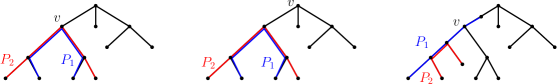
Figure 10: Three distinct placements of $v$. On the left, $v$ belongs to $P_{1}\cap P_{2}$, in the middle, $v$ does not belong to $P_{1}\cup P_{2}$, and on the right, $v$ belongs to exactly one of $P_{1}$ and $P_{2}$.

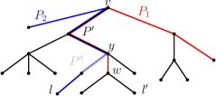
Figure 11: (a) The composition of the matrix $M$. (b) An interleaving pair of an $s$-cap and $b$-cap $P_{1}$ and $P_{2}$ corresponding to a restriction on a desired cyclic ordering of the leaves of $G$ involving a leaf $l^{\prime}$ that was “trimmed” while processing $(G_{y},\gamma)$.

The PC-tree algorithm processes $M$ from the top row by row. Enforcing an ambiguous symbol below every ambiguous symbol in $M_{y}^{\prime}$ corresponds to “trimming” $G$ by shortening every path $P$ joining $y$ with a leaf $l$ in $G_{y}$ limited by the interval corresponding to the currently processed row so that $P$ ends in the parent of $l$ in $G^{\prime}$. Note that we never “trim” the path starting at $y$ going towards its parent in $G^{\prime}$, when processing $(G_{y},\gamma)$, since such a path can be limited only by an interval strictly containing $I_{y}$. Also whenever we “trim” a path starting at $y$ we keep at least four paths starting at $y$, and thus, at least three paths going from $y$ towards leaves. Thus, if $w$, the other end vertex of $P_{\alpha\beta}$ than $v$, is not a descendant of $y$, there exists at least one column $c$ of $M_{y}^{\prime}$ such that $c$ $v$-represents the path $P_{\alpha\beta}$ and $c$ does not contain an ambiguous symbol in $M_{y}^{\prime}$. Unfortunately, if $w$ is a descendant of $y\not=v$, we could “trim” all the leaves that are descendants of $w$. In this case we would like to argue similarly as in the case of a subdivided star that by introducing an ambiguous symbol in $M$ in the row corresponding to $(s,b)$ of $M_{v}^{\prime}$ in all the columns $v$-representing $P_{\alpha\beta}$, we do not disregard required restrictions imposed on the order of leaves of $G$ by our characterization.

Let $y$ be a descendant of $v$ or equal to $v$. Suppose that we “trimmed” a descendant $l^{\prime}$ of $w$ or $w$ (if $w$ is a leaf) that is a descendant of $y$, while processing $(G_{y},\gamma)$ that appears, of course, before $(G_{v},\gamma)$ in our order or equals $(G_{y},\gamma)$. Let $L_{z}(s^{\prime\prime},b^{\prime\prime})$ and $L_{z}^{\prime}(s^{\prime\prime},b^{\prime\prime})$, respectively, be defined analogously as $E(s^{\prime\prime},b^{\prime\prime})$ and $E^{\prime}(s^{\prime\prime},b^{\prime\prime})$ in Section 5.1 for some $(G_{z},T)$ with leaves of $G$ playing the role of the edges incident to the center of the star and some $s^{\prime\prime}$ and $b^{\prime\prime}$, $s^{\prime\prime}<b^{\prime\prime}$. We also have an order corresponding to (1) for every $(G_{z},T)$. By reversing the order of clusters, without loss of generality we can assume that $w$ is an end vertex of $P_{1}$ which is an $s$-cap. Refer to Figure 12(a). If $\gamma(w)\in I_{y}$ then $w$ cannot be a descendant of $y$, since we have $I_{y}\subseteq(\min(P_{1}\setminus w),\max(P_{1}\setminus w))$ and $w\not\in(\min(P_{1}\setminus w),\max(P_{1}\setminus w))$. Thus, $\gamma(w)\not\in I_{y}$, and hence, $s\not\in I_{y}$. Moreover, $s<\min(I_{y})$, since $P_{1}$ is an $s$-cap. Since the descendant $l^{\prime}$ of $w$ was “trimmed” while processing $(G_{y},\gamma)$ by (1) there exists $L_{y}(s^{\prime},b^{\prime})$ for some $s^{\prime},b^{\prime}$ not containing $l^{\prime}$. Since the interval $(s^{\prime},b^{\prime})$ does not strictly contain $I_{y}$, contains $s$, and $s<\min(I_{y})$ we have $s^{\prime}\not\in I_{y}$, $s^{\prime}<s$ and $b^{\prime}\in I_{y}$. Moreover, if $y\not=v$ for some row of $M_{y}^{\prime}$ we have the corresponding $L_{y}(s,b^{\prime})$ containing $l^{\prime}$ since there exist at least two paths in $G_{y}$ from $y$ whose initial pieces correspond to the path from $y$ toward its parent as $v$ has degree at least three. Note that $L_{y}(s,b^{\prime})$ can contain only descendants of $y$. We claim the following (the proof is postponed until later)

$${L_{y}(s,b^{\prime})\subseteq L_{v}(s,b)\ \mathrm{and}\ L_{y}^{\prime}(s,b^{\prime})\supseteq L_{v}^{\prime}(s,b)}$$ (3)

Now, by using (3) we can extend the double-induction argument from Lemma 5.5.

In the same manner as in the previous section $R_{i}$ and $L_{i}$ correspond to the $i^{\mathrm{th}}$ row of $M^{\prime}$. We define $\mathcal{S}^{\prime}$ recursively as $\mathcal{S}_{m}^{\prime}$, $m$ is the number of rows of $M^{\prime}$, where $\mathcal{S}_{1}^{\prime}=\{L_{1}^{\prime},R_{1}^{\prime}|\ L_{1}^{\prime}=L_{1},\ R_{1}^{\prime}=R_{1}\}$ and $\mathcal{S}_{j}^{\prime}=\mathcal{S}_{j-1}\cup\{L_{j}^{\prime},R_{j}^{\prime}|\ L_{j}^{\prime}=L_{j}\cap(L_{j-1}^{\prime}\cup R_{j-1}^{\prime}),R_{j}^{\prime}=R_{j}\cap(L_{j-1}^{\prime}\cup R_{j-1}^{\prime})\}$. Let $S_{j,0}=L_{j}^{\prime}\cup R_{j}^{\prime}$. We need, in fact, to apply the condition (3) only when a new leaf $l^{\prime}$, such that $S_{j,k}=S_{j,k}\cup\{l^{\prime}\}$, added to $S_{j,k-1}$ (playing the role of the edge $e$ from the proof of Lemma 5.5) is the only descendant of $w$ in ${S}_{j,k}$. For the other descendants of $w$, $M_{G}$ forces the corresponding restriction. More formally, we need to show that a cyclic ordering of leaves $\mathcal{O}$ respecting restrictions imposed by the first $j-1$ rows, and the columns corresponding to $S_{j,k-1}$ in the $j^{\mathrm{th}}$ row, respects also restrictions imposed by the columns corresponding to $S_{j,k}$ in the $j^{\mathrm{th}}$ row. Let $\{l^{\prime}l_{1}\}\{l_{2}l_{3}\}$ be such a restriction for a leaf $l^{\prime}$ trimmed the most recently similarly as for $e$ in the case of subdivided stars. Let the restriction $\{l^{\prime}l_{1}\}\{l_{2}l_{3}\}$, $l_{1}\in L_{v}(s,b)\setminus L_{y}(s,b^{\prime})$, $l^{\prime}\in L_{v}(s,b)$ and $l_{2},l_{3}\in L_{v}^{\prime}(s,b)$, induced by $S_{j,k}$ in the $j^{\mathrm{th}}$ row correspond to pair of an $s$-cap $P_{1}$ and $b$-cup $P_{2}$, where the leaf $l^{\prime}$ $v$-represents a sub-path $P_{\alpha\beta}$ (for $v$ and $P_{\alpha\beta}$ defined as above) of $P_{1}$ ending in $w$ such that $\gamma(w)=s$.

Figure 12: (a) The interval corresponding to $P\setminus\{w\}$ containing $I_{y}$. (b) ) The interval corresponding to $P$ containing $I_{w^{\prime}}$.

First, we assume that $y=v$. First, note that $l_{2},l_{3}\in E_{v}^{\prime}(s,b^{\prime})$ by (2). We proceed by the same argument as in Lemma 5.5, since we have (1) for $G_{v}$. Here, $s,s^{\prime},b$ and $b^{\prime}$, respectively, plays the role of $s,s_{\alpha,\beta},b$ and $b_{\alpha}$. After we find $l^{\prime\prime}\in L_{v}(s,b^{\prime})$ that was “trimmed” after $l^{\prime}$ by induction hypothesis we have $\{l^{\prime}l^{\prime\prime}\}\{l_{2}l_{3}\}$ and $\{l^{\prime\prime}l_{1}\}\{l_{2}l_{3}\}$. Thus, by Observation 5.2 we are done. The only problem could be that we cannot find a leaf $l^{\prime\prime}\in L_{v}(s,b^{\prime})$ (analogous to the edge $g$) in the proof of Lemma 5.5 that was not “trimmed” before $l^{\prime}$ since all such leaves could be potentially “trimmed” while processing previous $(G_{y^{\prime}},T)$. However, recall that we “trim” only descendant of such $y^{\prime}$ while processing $(G_{y^{\prime}},T)$. We show that we can pick $l^{\prime\prime}$ such that this does not happen.

Refer to Figure 12(b). Indeed, consider the path from $v$ to its descendant $w^{\prime}$ that is an ancestor of $l^{\prime\prime}$ such that $w^{\prime}$ is an end vertex of an $s^{\prime}$-cap witnessing presence of $l^{\prime\prime}$ in $L_{v}(s^{\prime},b^{\prime})$. Among all possible choices of $l^{\prime\prime}$ and $w^{\prime}$, where, of course $l^{\prime\prime}$ is in the subtree rooted at $w^{\prime}$, let us choose the one minimizing $i$ such that the subtree rooted at $w^{\prime}$ contains a vertex in the $i^{\mathrm{th}}$ cluster. Moreover, we assume that $l^{\prime\prime}$ can be reached from $w^{\prime}$ by following a path passing through the vertex in the $i^{\mathrm{th}}$ cluster. Let $P^{\prime}$ denote the path between $v$ and $w^{\prime}$. Let $w^{\prime\prime}$ be an ancestor of $w$ that belongs to $V(G^{\prime})$ and is not an ancestor of $v$. (For other choices of $w^{\prime\prime}$ we cannot trim $l^{\prime\prime}$ while processing $G_{w^{\prime\prime}}$.) If $v=w^{\prime\prime}$ we show that we cannot “trim” $l^{\prime\prime}$ while processing $G_{w^{\prime\prime}}$ by the argument from Lemma 5.5. Otherwise, suppose that $w^{\prime\prime}\not=v$. Since $I_{w^{\prime\prime}}\subseteq(\min(P^{\prime}),\max(P^{\prime}))$ and $b_{\alpha}\not\in(\min(P^{\prime}),\max(P^{\prime}))$, we cannot “trim” the descendant $l^{\prime\prime}$ of $w^{\prime}$ while processing $(G_{w^{\prime\prime}},T)$. For otherwise $l^{\prime\prime}$ is a ✁ and we would get into a contradiction with the choice of $w^{\prime}$, since there exists a descendant $l^{\prime\prime\prime}$ of $w^{\prime\prime}$ in a cluster with the index smaller than $i$ good for us. The choice of $w^{\prime\prime}$ and $l^{\prime\prime\prime}$ is good since the interval corresponding to the row of $M$ with the maximal index, in which a column of the leaf $l^{\prime\prime}$ has 0 or 1, does not strictly contain $I_{w^{\prime\prime}}$, and thus, the path from $v$ towards $l^{\prime\prime\prime}$ that ends in the cluster $s^{\prime}$ never visits $b^{\prime}$ cluster.

Second, we assume that $y\not=v$. In this case we also have that $l_{2},l_{3}\in E_{y}^{\prime}(s,b^{\prime})$ by (3). We again repeat the argument from Lemma 5.5 in the same manner as for the case $y=v$. Here, again $s,s^{\prime},b$ and $b^{\prime}$, respectively, plays the role of $s,s_{\alpha,\beta},b$ and $b_{\alpha}$. Also a leaf $l^{\prime\prime}\in L_{y}(s,b^{\prime})$ that was not “trimmed” before $l^{\prime}$ playing the role of $g$ is found by the analysis in the previous paragraph, where $y$ plays the role of $v$.

If $l^{\prime}$ is not a descendant of $v$, recall that there exists at least one “untrimmed” leaf $l^{\prime\prime}$ such that $l^{\prime\prime}$ $v$-represents the path $P_{\alpha\beta}$. Then by induction hypothesis a restriction $\{l^{\prime\prime}l_{1}\}\{l_{2}l_{3}\}$ witnessed by $(s,b)$ corresponding to the $j^{\mathrm{th}}$ row gives the desired restriction $\{l^{\prime}l_{1}\}\{l_{2}l_{3}\}$ on $\mathcal{O}$ by Observation 5.2, since we have $\{l^{\prime\prime}l^{\prime}\}\{l_{2}l_{3}\}$ by $M_{G}$.

It remains to prove (3). Refer to Figure 11(b). If $v=y$ we are done by the argument in Lemma 5.5. Thus, we assume that $y\not=v$. We start by proving the first relation $L_{y}(s,b^{\prime})\subseteq L_{v}(s,b)$. If a leaf descendant $l$ of $y$ is in $L_{y}(s,b^{\prime})$ then $l\in L_{v}(s,b)$, since $b>b^{\prime}>\gamma(y)$ by $b^{\prime}\in I_{y},b\not\in I_{y}$, and $s\not\in(\min(P^{\prime}),\max(P^{\prime}))$, where $P^{\prime}$ is a path between $y$ and $v$. Then the corresponding witnessing path from $y$ towards $l$ of the fact $l\in L_{y}(s,b)$ can be extended by $P^{\prime}$ to the path witnessing $l\in L_{v}(s,b^{\prime})$. In order to prove the second relation $L_{y}^{\prime}(s,b^{\prime})\supseteq L_{v}^{\prime}(s,b)$ we first observe that $L_{y}^{\prime}(s,b^{\prime})$ contains all the leaves that are not descendants of $y$, since $b^{\prime}\in I_{y}$. On the other hand, if a leaf descendant $l$ of $y$ is in $L_{v}^{\prime}(s,b)$ then $l\in L_{y}^{\prime}(s,b^{\prime})$, since the corresponding witnessing path from $v$ toward $l$ of the fact $l\in L_{v}^{\prime}(s,b)$ contains a sub-path $P^{\prime\prime}$ starting at $y$ and ending in the cluster $b^{\prime}$ due to $b>b^{\prime}>\gamma(y)$ witnessing $l\in L_{y}^{\prime}(s,b^{\prime})$.

Thus, if the 0–1 matrix $M$ with ambiguous symbols has circular ones property then there exists an embedding of $G$ such that every interleaving pair is feasible, and hence, by Theorem 3.1 graph $(G,\gamma)$ admits an $x$-bounded embedding.   

6 Theta graphs

In this section we extend result from the previous one to the class of $x$-bounded drawings whose underlying abstract graph is a theta graph defined as a union of internally vertex disjoint paths joining a pair of vertices that we call poles. Hence, in the present section $(G,\gamma)$ is such that $G$ is a theta graph. Similarly as in Section 5 in what follows we assume $(*)$.

Our efficient algorithm for testing $x$-bounded embeddability of $(G,\gamma)$ relies on the work of Bläsius and Rutter [5]. We refer the reader unfamiliar with this work to the paper for necessary definitions. Thus, our goal is to reduce the problem to the problem of finding an ordering of a finite set that satisfies constraints given by a collection of PC-trees.

The construction of the corresponding instance $\mathcal{I}$ of the simultaneous PC-ordering for the given $(G,\gamma)$ is inspired by [5, Section 4.2]. Thus, the instance consists of a star $T_{C}$ having a P-node in the center (consistency tree), and a collection of embedding trees $T_{0},\ldots,T_{m}$ constructed analogously as in Section 5. The DAG (directed acyclic graph) representing $\mathcal{I}$ contains edges $(T_{0},T_{C},\varphi_{1})$, $(T_{0},T_{C},\varphi_{2})$, and $(T_{i},T_{i+1},\phi_{i})$ for $i=0,\ldots,m-1$  . Tree $T_{0}$ (see Figure 13) will consist, besides leaves and their incident edges, only of a pair of $P$-nodes joined by an edge. It follows that the instance is solvable in a polynomial time by [5, Theorem 3.3 and Lemma 3.5] The running time follows by [5, Theorem 3.2].

Figure 13: The theta-graph $G$ (left) and the PC-tree $T_{0}$ in its corresponding $\mathcal{I}$ instance.

Description of $(T_{0},T_{C},\varphi_{1})$, $(T_{0},T_{C},\varphi_{2})$.

Let $u$ and $v$ denote the poles of $G=(V,E)$. Let $e_{1},\ldots,e_{n}$ denote the edges incident to $u$. Let $f_{1},\ldots,f_{n}$ denote the edges incident to $v$. We assume that $e_{i}$ and $f_{i}$ belong to the same path $P_{i}$ between $u$ and $v$. The non-leaf vertices of $T_{0}$ are $P$-nodes $u$ and $v$, corresponding to $u$ and $v$ of $G$, joined by an edge. The $P$-node $u$ is adjacent to $n$ leaves and $v$ is adjacent to $n-1$ leaves. The tree $T_{C}$ is a PC-tree with a single $P$-node and $n$ leaves. The map $\varphi_{1}$ maps injectively every leaf of $T_{C}$ except one to a leave adjacent to $u$ the remaining leaf is mapped to an arbitrary leave of $v$. The map $\varphi_{2}$ maps injectively every leaf of $T_{C}$ except one to a leave adjacent to $v$ the remaining leaf is mapped arbitrarily such that the map is injective.

Let $I_{i}=(\min(P_{i}),\max(P_{i}))$ for every $i=1,\ldots,n$. Let $I_{j}$ be chosen so that $I_{i}\subseteq I_{j}$ implies $i=j$. Thus, $I_{j}$ is spanning a minimal number of clusters among $I_{i}$’s. Let $I_{\alpha}:=I_{j}$ and $P_{\alpha}:=P_{j}$. The leaves of $\varphi_{1}$ are mapped to the leaves of $u$ corresponding to edges incident to $u$ except for $e_{\alpha}$ and a single leave corresponding to the position of the the outer-face, and we have the analogous compatible correspondence for $\varphi_{2}$ except that $v$ has no leave representing the outer-face that $\varphi_{2}$ avoids. Since $T_{C}$ is the consistency PC-tree, the inherited cyclic orders of end pieces of paths $P_{i}$ corresponding to $\varphi_{1}$ and $\varphi_{2}$ have opposite orientations. Thus, one of the arcs $(T_{0},T_{C},\varphi_{1})$ and $(T_{0},T_{C},\varphi_{2})$ is orientation preserving and the other one orientation reversing.

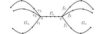
Figure 14: The graph $G^{\prime}$ consisting of $G_{u}$, $G_{v}$ and $P_{\alpha}$.

Description of $(T_{i},T_{i+1},\phi_{1})$.

We will construct $(G^{\prime},\gamma^{\prime})$, where $G^{\prime}$ is a tree, (see Figure 14) yielding desired embedding trees $T_{i}$’s, for $i>0$, in $\mathcal{I}$. The tree $G^{\prime}$ is obtained as the union of a pair of vertex disjoint subdivided star $G_{u}$ and $G_{v}$, and the path $P_{\alpha}$ (defined in the previous paragraph) joining the centers of $G_{u}$ and $G_{v}$. The graph $G_{u}$ is isomorphic to $G\setminus(\{v\}\cup E(P))$ and $G_{v}$ is isomorphic to $G\setminus(\{u\}\cup E(P))$. The assignment $T^{\prime}$ of the vertices to clusters is inherited from $(G,\gamma)$.

The path $T_{0}T_{1}\ldots T_{m}$ in the DAG of $\mathcal{I}$ corresponds to a variant $M^{\prime}$ of the matrix $M$ from Section 5 constructed for $G^{\prime}$ with additional rows between $M_{G^{\prime}}^{\prime}$ and $M_{u}^{\prime}$. The leaves of $T_{1}$ corresponds to the columns of $M^{\prime}$.

(i) The tree $T_{0}$ corresponds to $M_{G^{\prime}}$.
(ii) $T_{1}$ takes care of the trapped vertices (that we did not have to deal with in the case of trees).
(iii) $T_{1},\ldots,T_{l}$, for some $l$, corresponds to $M_{u}^{\prime}$, and $T_{l+1},\ldots,T_{m}$, to $M_{v}^{\prime}$.

The described trees naturally correspond to constraints on the rotations at $u$ and $v$. Before we proceed with proving the correctness of the algorithm we describe the last missing piece of the construction, the PC-tree $T_{1}$.

Description of $T_{1}$.

The PC-tree $T_{1}$ corresponds to the set of constraints given by the following 0–1 matrix $M^{\prime\prime}$. The leaves corresponding to $e_{\alpha}$ are all the leaves incident to $v$, and the leaves corresponding to $f_{\alpha}$ are the leaves incident to $u$. The correspondence of the remaining edges incident to $u$ and $v$ to the columns of $M^{\prime\prime}$ is given by their correspondence with leaves of $T_{1}$ explained above. The matrix $M^{\prime\prime}$ has only zeros in the column representing the outer-face in the rotation at $u$. Let us take the maximal subset of edges incident to $u$, whose elements $e_{1},\ldots,e_{n^{\prime}}$ are ordered (we relabel the edges appropriately) such that $i<i^{\prime}$ implies $\min(P_{i})<\min(P_{i^{\prime}})$. For every $j$, $1\leq j\leq n^{\prime}$, we introduce a row having zeros in the columns corresponding to $e_{1},\ldots,e_{j}$ and columns corresponding to $e_{i}$ for which there exists $i^{\prime}$, $1\leq i^{\prime}\leq j$, $\min(P_{i})=\min(P_{i^{\prime}})$, and having ones in the remaining columns except the one representing the outer-face.

Let us take the maximal subset of edges incident to $u$, whose elements $e_{1},\ldots,e_{n^{\prime}}$ are ordered such that $i<i^{\prime}$ implies $\max(P_{i})>\max(P_{i^{\prime}})$. For every $j$, $1\leq j\leq{n^{\prime}}$, we introduce a row having zeros in the columns corresponding to $e_{1},\ldots,e_{j}$ and columns corresponding to $e_{i}$ for which there exists $i^{\prime}$, $1\leq i^{\prime}\leq j$, $\max(P_{i})=\max(P_{i^{\prime}})$, and having ones in the remaining columns except the one representing the outer-face.

A trapped vertex $v^{\prime}$ on $P_{i}$ in a cycle $C$ consisting of $P_{i^{\prime}}$ and $P_{i^{\prime\prime}}$ would violate a constraint $\{e_{i}^{\prime}e_{i}^{\prime\prime}\}\{e_{i}e_{0}\}$, where $e_{0}$ is the dummy edge on the outer-face enforced by $T_{1}$.

It remains to prove that the instance $\mathcal{I}$ is a if and only if any corresponding witnessing order of the leaves yields an isotopy class of $G$ that contains an $x$-bounded embedding of $(G,\gamma)$ by Theorem 3.1. This might come as a surprise since some constraints on the rotation system enforced by the original instance $(G,\gamma)$ might be missing in $\mathcal{I}$, and on the other hand some additional constraints might be introduced.

Theorem 6.1.

The instance $\mathcal{I}$ is a “yes” instance if and only if $(G,\gamma)$ admits an $x$-bounded embedding.

Proof.

By the discussion above it remains to prove that the order constraints corresponding to the trees $T_{2},\ldots,T_{m}$ are all the constraints given by the infeasible interleaving pairs of paths $P_{1}^{\prime}$ and $P_{2}^{\prime}$, and possibly additional constraint enforced by trapped vertices.

First, we note that no additional constraints are introduced due to the fact that we might have two copies of a single vertex of $G$ in $G^{\prime}$. Indeed, such a constraint corresponds to a pair of paths $P_{1}^{\prime}$ and $P_{2}^{\prime}$ intersecting in the copy of $P_{\alpha}$, such that their union contains at least one whole additional $P_{l}$, for $l\not=\alpha$. However, in this case it must be that the two copies of a single vertex in the union of $P_{1}^{\prime}$ and $P_{2}^{\prime}$ are the endpoints of, let’s say $P_{1}^{\prime}$. Thus, the constraint of $P_{1}^{\prime}$ and $P_{2}^{\prime}$ exactly prevents end vertices of $P_{2}^{\prime}$ from being trapped in the cycle of $G$ obtained by identifying the end vertices of $P_{1}^{\prime}$.

Figure 15: The paths $P_{1}^{\prime}$ and $P_{2}^{\prime}$ meeting in $P_{l}$ such that $I_{l}=(\min(P_{l}),\max(P_{l}))$ contains $I_{\alpha}$ (left). The corresponding cyclic order of the leaves corresponding to the edges incident to $u$ and $v$ captured by $T_{0}$ (right).

If $P_{1}^{\prime}$ and $P_{2}^{\prime}$ intersect exactly in the vertex $u$ or $v$ the corresponding constraint is definitely captured. Similarly, if $P_{1}^{\prime}$ and $P_{2}^{\prime}$ intersects exactly in the path $P_{\alpha}$. Otherwise, if $P_{1}^{\prime}$ and $P_{2}^{\prime}$ intersects in a path $P_{l}$ such that $I_{l}=(\min(P_{l}),\max(P_{l}))$ contains $I_{\alpha}$, we have the corresponding constraint present implicitly.

Refer to Figure 15. Indeed, an ordering $\mathcal{O}$ of the columns of $M^{\prime}$ witnessing that $\mathcal{I}$ is a “yes” instance satisfies $\{e_{\alpha}e_{l}\}\{e_{p}e_{q}\}$ by $T_{1}$, where $e_{p}$ and $e_{q}$, respectively, is the edge incident to $u$ belonging to $P_{1}^{\prime}$ and $P_{2}^{\prime}$, and also $\mathcal{O}$ satisfies $\{f_{\alpha}f_{l}\}\{f_{r}f_{s}\}$, by the consistency tree $T_{C}$, where $f_{r}$ and $f_{s}$, respectively, is the edge incident to $v$ belonging to $P_{1}^{\prime}$ and $P_{2}^{\prime}$, Moreover, by the constraint obtained from the union of paths $P_{1}^{\prime}$ and $P_{2}^{\prime}$ by replacing $P_{l}$ with $P_{\alpha}$, we obtain that $\mathcal{O}$ satisfies $\{e_{p}f_{r}\}\{e_{q}f_{s}\}$. By the constrains of $T_{0}$ it then follows that in the rotation at $u$ the edges $e_{l},e_{p},e_{q}$ appear w.r.t. to this order with the opposite orientation as $f_{l},f_{r},f_{s}$. Hence, the pair of $P_{1}^{\prime}$ and $P_{2}^{\prime}$ is feasible with respect to $\mathcal{O}$.

Figure 16: The paths $P_{1}^{\prime}$ and $P_{2}^{\prime}$ meeting in $P_{l}$ such that $I_{l}=(\min(P_{l}),\max(P_{l}))$ does not contain $I_{\alpha}$ (left). The corresponding cyclic order of the leaves corresponding to the edges incident to $u$ and $v$ captured by $T_{0}$ (right).

Finally, if $I_{l}$ does not contain $I_{\alpha}$, the previous argument does not apply if the interval
$(\min(P_{1}^{\prime}\cup P_{2}^{\prime}),\max(P_{1}^{\prime}\cup P_{2}^{\prime}))$ does not contain $I_{\alpha}$. We assume that

$$\max(P_{1}^{\prime}\cup P_{2}^{\prime})>\max(I_{l})>\max(I_{\alpha})\geq\min(I_{l})>\min(P_{1}^{\prime}\cup P_{2}^{\prime}))\geq\min(I)$$

and handle the remaining cases by the symmetry. We assume that $P_{1}^{\prime}$ is a cap passing through edges $e_{p}$ and $f_{r}$. We assume that $P_{2}^{\prime}$ is a cup passing through edges $e_{q}$ and $f_{s}$.

The ordering $\mathcal{O}$ satisfies $\{e_{p}e_{\alpha}\}\{e_{l}e_{q}\}$ and $\{f_{r}f_{\alpha}\}\{f_{l}f_{s}\}$. By $T_{1}$ we have $\{e_{q}e_{s}\}\{e_{\alpha}e_{l}\}$. By $T_{0}$ and $T_{C}$, $e_{i}$’s and $f_{i}$’s appear consecutively and they are reverse of each other in $\mathcal{O}$. Thus, we have $\{e_{l}f_{l}\}\{e_{q}f_{s}\}$.

Refer to Figure 16. A simple case analysis reveals that the observations in the previous paragraph gives us the following. If $\{e_{p}f_{r}\}\{e_{q}f_{s}\}$ is satisfied by $\mathcal{O}$, then $\mathcal{O}$ satisfies $\{e_{l}f_{l}\}\{e_{p}e_{q}\}$ if and only if $\{e_{l}f_{l}\}\{f_{s}f_{r}\}$. On the other hand, if $\{e_{p}f_{r}\}\{e_{q}f_{s}\}$ is not satisfied by $\mathcal{O}$, then $\mathcal{O}$ satisfies $\{e_{l}f_{l}\}\{e_{p}e_{q}\}$ if and only if it does not satisfy $\{e_{l}f_{l}\}\{f_{s}f_{r}\}$. By the symmetry there are four cases to check (see Figure 17). Using the language of the formal logic the previous fact about $\mathcal{O}$ is expressed by the following formula.

$$\{e_{p}f_{r}\}\{e_{q}f_{s}\}\Rightarrow(\{e_{l}f_{l}\}\{e_{p}e_{q}\}\Leftrightarrow\{e_{l}f_{l}\}\{f_{s}f_{r}\})\ \bigwedge\ \neg\{e_{p}f_{r}\}\{e_{q}f_{s}\}\Rightarrow(\{e_{l}f_{l}\}\{e_{p}e_{q}\}\Leftrightarrow\neg\{e_{l}f_{l}\}\{f_{s}f_{r}\})$$

Figure 17: The orderings of the leaves in $T_{0}$ corresponding to the true assignment of the propositional formula. Since only $e_{p},e_{q},f_{r},f_{s},e_{l}$ and $e_{l}$ appear in the formula. We can fix $e_{q},f_{s},e_{l}$ and $f_{l}$ and use top-bottom symmetry.

By the formula, it easily follows that the orientation around $u$ and $v$, respectively, of the edges $e_{l},e_{p},e_{q}$ and $f_{l},f_{r},f_{s}$ is opposite of each other and we are done.   

7 Beyond theta graphs and trees

One might wonder if our algorithm and/or Hanani–Tutte variant for theta graphs can be extended to arbitrary planar graphs.

It is tempting to consider the following definition of $(G^{\prime},\gamma^{\prime})$ corresponding to an instance $(G,\gamma)$. Let us suppress every vertex of degree two in $G$. Let $G^{\prime\prime}$ denote the resulting multi-graph. Each edge $e$ in $G^{\prime\prime}$ has a corresponding path $P:=P(e)$ in $G$ (which is maybe just equal to $e$). Let us assign a non-negative weights $w(e)$ to every edge $e$ of $G^{\prime\prime}$ equal to $\max(P)-\min(P)$. Let $G^{\prime\prime\prime}$ denote the minimum weight spanning tree of $G^{\prime\prime}$.

The tree $G^{\prime}$ is obtained as the union of the subgraph of $G$ corresponding to $G^{\prime\prime\prime}$, and pairs of copies of paths $P(e)$, for each $e=uv$, where one copy of each pair is attached to $u$ and the other one to $v$, but otherwise disjoint from $G^{\prime\prime\prime}$. The assignment of the vertices to the clusters in $(G^{\prime},\gamma^{\prime})$ is inherited from $(G,\gamma)$.

Note that if $G$ is a theta graph the resulting $G^{\prime}$ is almost equal to the one defined in the previous subsections, except that earlier we shortened copies of $P(e)$’s for $e$ not in $G^{\prime\prime\prime}$ so that they do not contain one end vertex of $P(e)$. In the case of theta graphs this does not make a difference, but for more general class of graphs our new definition of $G^{\prime}$ might be more convenient to work with.

Now, we would like to use the construction of [5, Section 4.1] enriched by the constraints of $(G^{\prime},\gamma^{\prime})$, and other necessary contraptions if the graph is not two-connected.

If the graph is two-connected it seems plausible that it is enough if we generalize our construction of $T_{1}$ (taking care of trapped vertices), and prove that the constraints of $(G^{\prime},\gamma^{\prime})$ together with other constraints account for all infeasible interleaving pairs of path. To construct $T_{1}$ is not difficult, since we just repeat our construction of the matrix corresponding to $T_{1}$ for each consistency tree corresponding to a pair of vertices participating in the two-cut, and combine the resulting matrices.

Then it seems that the only challenging part is to adapt the last paragraph in the proof of Theorem 6.1, which does not seem to be beyond reach. To this end it is likely that a more efficient version of the characterization in Theorem 3.1 is also needed, where by “more efficient” we mean a version that restricts the set of interleaving pairs of paths considered. This should be possible, since in our proofs for trees and theta graphs a considerably restricted subset of interleaving feasible pairs implied feasibility for the rest.

When the graph $G$ is not guaranteed to be two-connected, generalizing $T_{1}$ does not seem to be a way to go. However, the general strategy of combining simultaneous PC-orderings with our characterization could work, if the constraints preventing an occurrence of trapped vertices and infeasible interleaving pairs are treated simultaneously using a more efficient version of Theorem 3.1.

8 Open problems

We also wonder if the running time in Theorem 1.6 and 1.7 can be improved, and if our main result, Theorem 1.2, can be extended to radial [3] or cyclic [2, 14] setting, to higher genus surfaces and what are its higher dimensional analogues.

Acknowledgment.

We would like to express our sincere gratitude to the organizers and participants of the 11th GWOP workshop, where we could discuss the research problems treated in the present paper. In particular, we especially benefited from the discussions with Bettina Speckmann, Edgardo Roldán-Pensado and Sebastian Stich.

Furthermore, we would like to thank Ján Kynčl for useful discussions at the initial stage of this work and many useful comments, Gábor Tardos for comments that helped to improve the presentation of the results, and to Arkadij Skopenkov for telling us about [33]. An adaptation of the ideas from this work and also from [22], resulted in a tremendous simplification of the proof of our main result, Theorem 3.1.

References

- [1] Patrizio Angelini, Giordano Da Lozzo, Giuseppe Di Battista, and Fabrizio Frati. Strip planarity testing. In Stephen Wismath and Alexander Wolff, editors, Graph Drawing, volume 8242 of Lecture Notes in Computer Science, pages 37–48. Springer International Publishing, 2013.
- [2] Patrizio Angelini, Giordano Da Lozzo, Giuseppe Di Battista, Fabrizio Frati, Maurizio Patrignani, and Ignaz Rutter. Beyond level planarity. 2015. arXiv:1510.08274.
- [3] Christian Bachmaier, Franz J. Brandenburg, and Michael Forster. Radial level planarity testing and embedding in linear time. In Graph Drawing, volume 2912 of Lecture Notes in Computer Science, pages 393–405. 2004.
- [4] P. Bertolazzi, Giuseppe Di Battista, Giuseppe Liotta, and Carlo Mannino. Upward drawings of triconnected digraphs. Algorithmica, 12(6):476–497, 1994.
- [5] Thomas Bläsius and Ignaz Rutter. Simultaneous PQ-ordering with applications to constrained embedding problems. In Proceedings of the Twenty-Fourth Annual ACM-SIAM Symposium on Discrete Algorithms, SODA 2013, New Orleans, Louisiana, USA, January 6-8, 2013, pages 1030–1043, 2013. http://arxiv.org/abs/1112.0245.
- [6] Thomas Bläsius and Ignaz Rutter. A new perspective on clustered planarity as a combinatorial embedding problem. In Christian Duncan and Antonios Symvonis, editors, Graph Drawing, Lecture Notes in Computer Science, pages 440–451. 2014.
- [7] Kellogg S. Booth and George S. Lueker. Testing for the consecutive ones property, interval graphs, and graph planarity using PQ-tree algorithms. Journal of Computer and System Sciences, 13(3):335 – 379, 1976.
- [8] Peter Brass, Eowyn Cenek, Cristian A. Duncan, Alon Efrat, Cesim Erten, Dan P. Ismailescu, Stephen G. Kobourov, Anna Lubiw, and Joseph S.B. Mitchell. On simultaneous planar graph embeddings. Computational Geometry, 36(2):117 – 130, 2007.
- [9] Grant Cairns and Yury Nikolayevsky. Bounds for generalized thrackles. Discrete Comput. Geom., 23(2):191–206, 2000.
- [10] Reinhard Diestel. Graph Theory. Springer, New York, 2010.
- [11] Qing-Wen Feng, Robert F. Cohen, and Peter Eades. How to draw a planar clustered graph. In Ding-Zhu Du and Ming Li, editors, Computing and Combinatorics, volume 959 of Lecture Notes in Computer Science, pages 21–30. Springer Berlin Heidelberg, 1995.
- [12] Qing-Wen Feng, Robert F. Cohen, and Peter Eades. Planarity for clustered graphs. In Paul Spirakis, editor, Algorithms — ESA ’95, volume 979 of Lecture Notes in Computer Science, pages 213–226. Springer Berlin Heidelberg, 1995.
- [13] Radoslav Fulek. Towards the Hanani–Tutte theorem for clustered graphs. In Graph-Theoretic Concepts in Computer Science - 40th International Workshop, WG 2014, Nouan-le-Fuzelier, France, June 25-27, 2014. Revised Selected Papers, pages 176–188, 2014.
- [14] Radoslav Fulek. C-planarity of embedded cyclic c-graphs. 2016. arxiv:1602.01346v2.
- [15] Radoslav Fulek, Jan Kynčl, Igor Malinovic, and Dömötör Pálvölgyi. Clustered planarity testing revisited. Electronic Journal of Combinatorics, 22, 2015.
- [16] Radoslav Fulek, Michael Pelsmajer, Marcus Schaefer, and Daniel Štefankovič. Hanani-Tutte, monotone drawings and level-planarity. Thirty Essays in Geometric Graph Theory, J. Pach ed., pages 263–288, 2012.
- [17] Ashim Garg and Roberto Tamassia. On the computational complexity of upward and rectilinear planarity testing. SIAM J. Comput., 31(2):601–625, February 2002.
- [18] Haim Hanani. Über wesentlich unplättbare Kurven im drei-dimensionalen Raume. Fundamenta Mathematicae, 23:135–142, 1934.
- [19] Wen-Lian Hsu and Ross M. McConnell. PC-trees and circular-ones arrangements. Theoretical Computer Science, 296(1):99 – 116, 2003.
- [20] Michael Jünger, Sebastian Leipert, and Petra Mutzel. Level Planarity Testing in Linear Time, pages 224–237. Springer Berlin Heidelberg, Berlin, Heidelberg, 1998.
- [21] Thomas Lengauer. Hierarchical planarity testing algorithms. J. ACM, 36(3):474–509, 1989.
- [22] Piotr Minc. Embedding simplicial arcs into the plane. Topol. Proc. 22, pages 305–340, 1997.
- [23] J. Opatrny. Total ordering problem. SIAM Journal on Computing, 8(1):111–114, 1979.
- [24] János Pach and Géza Tóth. Which crossing number is it anyway? J. Combin. Theory Ser. B, 80(2):225–246, 2000.
- [25] János Pach and Géza Tóth. Monotone drawings of planar graphs. J. Graph Theory, 46(1):39–47, 2004. updated version: arXiv:1101.0967.
- [26] Michael J. Pelsmajer, Marcus Schaefer, and Despina Stasi. Strong Hanani–Tutte on the projective plane. SIAM Journal on Discrete Mathematics, 23(3):1317–1323, 2009.
- [27] Michael J. Pelsmajer, Marcus Schaefer, and Daniel Štefankovič. Removing even crossings. J. Combin. Theory Ser. B, 97(4):489–500, 2007.
- [28] Michael J. Pelsmajer, Marcus Schaefer, and Daniel Štefankovič. Removing even crossings on surfaces. European Journal of Combinatorics, 30(7):1704–1717, 2009.
- [29] Marcus Schaefer. Hanani-Tutte and related results. To appear in Bolyai Memorial Volume.
- [30] Marcus Schaefer. Toward a theory of planarity: Hanani–Tutte and planarity variants. Journal of Graph Algorithms and Applications, 17(4):367–440, 2013.
- [31] Marcus Schaefer and Daniel Štefankovič. Block additivity of -embeddings. In Proceedings of 21st International Symposium on Graph Drawing, Bordeaux, France. to appear.
- [32] K Sieklucki. Realization of mappings. Fundamenta Mathematicae, 65(3):325–343, 1969.
- [33] Mikhail Skopenkov. On approximability by embeddings of cycles in the plane. Topology and its Applications, 134(1):1–22, 2003.
- [34] William T. Tutte. Toward a theory of crossing numbers. J. Combin. Theory, 8:45–53, 1970.
- [35] William Thomas Tutte. How to draw a graph. Proc. London Math. Soc, 13(3):743–768, 1963.