DSValidator : An Automated Counterexample Reproducibility
Tool for Digital Systems

Abstract.

An automated counterexample reproducibility tool based on MATLAB is presented, called DSValidator, with the goal of reproducing counterexamples that refute specific properties related to digital systems. We exploit counterexamples generated by the Digital System Verifier (DSVerifier), which is a model checking tool based on satisfiability modulo theories for digital systems. DSValidator reproduces the execution of a digital system, relating its input with the counterexample, in order to establish trust in a verification result. We show that DSValidator can validate a set of intricate counterexamples for digital controllers used in a real quadrotor attitude system within seconds and also expose incorrect verification results in DSVerifier. The resulting toolbox leverages the potential of combining different verification tools for validating digital systems via an exchangeable counterexample format.

1. Introduction

Digital systems (e.g., filters and controllers) consist of a mathematical operator that maps one signal into another signal using a fixed set of operations (diniz, ); they are used in several applications due to advantages over the analog counterparts, such as reliability, flexibility, and cost. However, there are disadvantages in the use of digital systems; since they are typically implemented in microprocessors, errors might be introduced due to quantizations and round-offs. The hardware choice, realizations (e.g., delta and direct forms), and implementation features (e.g., number of bits, fixed-point arithmetic) impact the digital system precision and performance (daes20161, ).

To detect errors in a digital system implementation, considering finite word-length (FWL) effects (fadali09, ; istepanianbook01, ), a model checking procedure based on satisfiability modulo theories (SMT) has been proposed in the literature, named as Digital System Verifier (DSVerifier) (dsverifier, ), which verifies digital filters and controllers represented by transfer functions and state-space equations (daes20161, ; Bessa16, ; monteiro2016, ; Abreu2016, ). DSVerifier checks properties related to overflow, limit cycle, stability, and minimum-phase in different digital system realizations and numerical formats.

Currently, there are several toolboxes in MATLAB to support digital system design (matlab-toolbox, ). For instance, the fixed-point designer toolbox provides data-types and tools for developing fixed-point digital systems. There are also other toolboxes implemented with different objectives, e.g., optimization, control system, and digital signal processing (matlab-toolbox, ). However, there is no toolbox to reproduce counterexamples in digital systems generated by verifiers, i.e., automatically reproduce a sequence of states that refutes a specific property in order to establish trust in a verification result.

There are verifiers to validate counterexamples using the witness validation approach, which reproduces the verification results by checking a given counterexample based on the graphml format (dirk2015, ). For instance, CPAchecker (cpachecker, ) and Ultimate Automizer (ultimate, ) employ the error-witness-driven program analysis technique to avoid false alarms produced by verifiers, i.e., given a witness for a problematic program path, they re-verify that the witness indeed violates the specification. However, those tools are currently unable to support the validation of systems that require fixed-point arithmetic, and consequently disregard FWL effects, which is needed to successfully validate implementation-level properties of typical digital systems.

Contributions. This paper describes and evaluates a novel MATLAB toolbox called DSValidator to automatically check whether a counterexample given by a verifier is reproducible. We propose a particular format to represent counterexamples, which can be used by other verifiers and MATLAB toolboxes. Here, a counterexample provides assignments to the digital system’s variables, which can be extracted to reproduce a given violation. This counterexample allows us to reproduce the failed property, providing concrete, lower-level details needed to simulate the digital system in MATLAB. DSValidator can validate counterexamples related to overflow, limit-cycle, stability, and minimum-phase. We show that DSValidator is able to reproduce a set of intricate counterexamples for digital controllers used in a real quadrotor attitude control system within seconds. DSValidator can also expose incorrect verification results in DSVerifier due to wrong computations of the system output.

Availability of Data and Tools. Our experiments are based on a set of publicly available benchmarks. All tools, benchmarks, videos, and results of our evaluation are available on a supplementary web page http://dsverifier.org/. In particular, DSValidator source code is available in a public repository located at https://github.com/ssvlab/dsverifier/tree/master/toolbox-dsvalidator.

2. DSValidator Digital System Reproducibility Engine

DSValidator is able to simulate digital controllers and filters considering implementation features (e.g., FWL effects and realizations) by taking into account a given counterexample provided by a verifier.

2.1. Digital System Representation

DSValidator supports digital systems (digital controllers and filters), represented by transfer functions, i.e., frequency domain equations that are able to represent input-to-output relations in a digital system. The following expression presents the general form of a digital system transfer function:

(1) $$H(z)=\frac{B(z)}{A(z)}=\frac{b_{0}+b_{1}z^{-1}+...+b_{M}z^{-M}}{a_{0}+a_{1}z^{-1}+...+a_{N}z^{-N}},$$

where $z^{-1}$ is called backward-shift operator; $A(z)$ and $B(z)$ are the denominator and numerator polynomials; and $N$ and $M$ represent the denominator and numerator polynomials order, respectively. Another representation is the difference equation, which can be described as

(2) $$y(n)=-\sum_{k=1}^{N}a_{k}y(n-k)+\sum_{k=0}^{M}b_{k}x(n-k).$$

Eq. (2) allows DSValidator to compute the system output $y(n)$ at the $n$-th instant (i.e., at time $t=n\cdot T$, where $T$ is the system sample time) using values of the past outputs and the present and past inputs (i.e., $x(n)$).

2.2. Counterexample Reproducibility for the Digital System Properties

2.2.1. Stability and Minimum-phase.

A digital system is stable iff all of its poles are inside the $z$-plane unitary circle; poles must have the modulus less than one. Minimum-phase is also a desirable property for digital systems. A digital system is a minimum-phase system iff all of its zeros are inside the $z$-plane unitary circle. The counterexample reproducibility for both minimum-phase and stability does not require DSValidator to compute output and states since polynomial analysis is performed, but FWL effects over the coefficients of Eq. (1) must be computed.

Definition 1.

(Finite Word-Length) $\mathcal{FWL}[\cdot]:\mathbb{R}^{N+M+2}\rightarrow Q[\mathbb{R}^{N+M+2}]$ function applies FWL effects to a polynomial vector representation, where $Q[\mathbb{R}]$ represents the quantized set of representable real numbers in the chosen implementation format.

Definition 2.

(Roots of a Polynomial) $\mathcal{R}[\cdot]:\mathbb{R}^{N+M+2}\rightarrow\mathfrak{S}$ function computes the set of roots of a polynomial, and $\mathfrak{S}$ is a family of sets. The poles of Eq. (1) is computed by $\mathcal{R}[A(z)]$, and the zeros are computed by $\mathcal{R}[B(z)]$.

Definition 3.

(Stability Reproducibility) DSValidator computes the $\mathcal{FWL}[A(z)]$ roots for stability reproduction. If any root has modulus equal or greater than one, then the system is unstable; otherwise, it is stable.

Definition 4.

(Minimum-phase Reproducibility) DSValidator computes the $\mathcal{FWL}[B(z)]$ roots for minimum-phase reproduction. If any root has modulus equal or greater than one, then the system is non minimum-phase; otherwise, it is minimum-phase.

2.2.2. Overflow

When an operation result exceeds the limited range of the processor’s word-length, overflow might occur in the output of the digital system realization, resulting in undesirable nonlinearities in the output. In order to reproduce an overflow counterexample, the output sequence must be computed for the given input sequence; the counterexample should contain an input sequence $x(n)$ that leads the digital system to overflow. DSValidator reads the counterexample provided by a given verifier, and then computes FWL effects over the coefficients, i.e., DSValidator computes $\mathcal{FWL}[A(z)]$ and $\mathcal{FWL}[B(z)]$ (cf. Definition 1).

After that, DSValidator checks the word-length representation limits, considering $n$-integer bits and $l$-fractional bits. The maximum representable value is computed as $2^{n-1}-2^{-l}$ and the minimum representable value is computed as $-2^{n-1}$. Then, Eq. (2) is iteratively unrolled for a given realization form, considering the input $x(n)$ (from the counterexample) to produce the output $y(n)$.

Definition 5.

(Realization Form) A realization form represents a template to implement a given digital system in software by using directly the coefficients of Eq. (1) in its implementation (daes20161, ).

Definition 6.

(Overflow reproducibility) DSValidator checks whether each system’s output is inside the word-length representation limits; the output does not lead to overflow if $-2^{n-1}<y(n)<2^{n-1}-2^{-l}$ is inside the word-length limits. A detected overflow violation must be similar to the counterexample indicated by the verifier; otherwise, the counterexample is not reproducible.

2.2.3. Limit Cycle Oscillation (LCO)

Limit cycle is defined by the presence of oscillations in the output, even when the input sequence is constant. LCO can be classified as granular or overflow.

Definition 7.

(Granular LCO) Granular limit cycles are autonomous oscillations due to round-offs in the least significant bits (diniz, ).

Definition 8.

(Overflow LCO) Overflow limit cycles appear when an operation results in overflow using the wrap-around mode (diniz, ).

To reproduce LCO counterexamples, constant inputs and initial states are used as test signals in DSValidator to compute the output sequence $y(n)$, considering a given realization form (cf. Definition 5). First, DSValidator obtains FWL effects on the numerator and denominator coefficients (cf. Definition 1). The constant input, initial states, and realization form are provided by a given counterexample and employed to compute $y(n)$ based on the fixed-point arithmetic and also to simulate the respective digital system in MATLAB.

Definition 9.

(LCO reproducibility) If the system’s output $y(n)$ provided by DSValidator leads to oscillations in the output with the same characteristics (i.e., amplitude and period) from that indicated by the verifier, then the LCO counterexample is reproducible; otherwise, the verifier presents an error.

In order to confirm the LCO absence, the algorithm proposed by Bauer (bauer, ; premaratne, ) was implemented in DSValidator. The aim of that algorithm is to exhaustively search for the absence of limit cycle; it is applicable to all direct form realizations, besides being independent on the quantization and system order. Therefore, Bauer’s method decides about the asymptotic stability of (linearly stable) digital systems, by employing an exhaustive search method. If it detects that a digital system is asymptotic stable, then the latter is limit cycle free; otherwise, it is susceptible to overflow or granular LCO.

3. Automated Counterexample Reproducibility for Digital Systems

3.1. Proposed Counterexample Format

DSValidator exploits counterexamples provided by verifiers (dsverifier, ; cbmc, ; esbmc, ); if there is a property violation, then the verifier provides a counterexample, which contains inputs and initial states that lead the digital system to a failure state. Fig. 1 shows an example of the present counterexample format related to an overflow LCO violation for the digital system represented by Eq. (3):

(3) $$H(z)=\frac{2002-4000z^{-1}+1998z^{-2}}{1-z^{-2}}.$$

⬇

1Property = LIMIT_CYCLE

2Numerator = { 2002, -4000, 1998 }

3Denominator = { 1, 0, -1 }

4X_Size = 10

5Sample_Time = 0.001

6Implementation = <13,3>

7Numerator (fixed-point) = { 2002, -4000, 1998 }

8Denominator (fixed-point) = { 1, 0, -1 }

9Realization = DFI

10Dynamical_Range = { -1, 1 }

11Initial_States = { -0.875, 0, -1 }

12Inputs = { 0.5, 0.5, 0.5, 0.5, 0.5, 0.5, 0.5, 0.5, 0.5, 0.5}

13Outputs = { 0, -1, 0, -1, 0, -1, 0, -1, 0, -1}

Figure 1. Proposed Counterexample Format Example.

The proposed counterexample format shown in Fig. 1 describes the violated property (represented by a string), transfer function numerator and denominator (represented by fixed-point numbers), bound (represented by an integer), sample time (represented by a fixed-point number), implementation aspects (integer and fractional bits represented by an integer), realization form (represented by a string), dynamical range (represented by an integer), initial states, inputs, and outputs (which are represented by fixed-point numbers). In particular, the counterexample provides the needed data to reproduce a given property violation via simulation in MATLAB.

DSValidator considers “.out” files to extract the counterexample and to transform them into MATLAB variables; those “.out” files are generated by the verifier after the digital system verification is performed. Currently, DSValidator is able to validate the minimum-phase, overflow, stability, and limit-cycle properties for a digital system that is represented by a transfer function. Additionally, DSValidator is able to employ $6$ direct and delta realization forms for digital systems: direct form I (DFI), direct form II (DFII), transposed direct form II (TDFII), delta direct form I (DDFI), delta direct form II (DDFII), and transposed delta direct form II (TDDFII) (daes20161, ).

3.2. Automated Counterexample Validation

There are five steps to automatically perform the automated counterexample validation in DSValidator. In step ($1$), DSValidator obtains the counterexample and then uses a shell script to extract the data related to the digital system, i.e., property, transfer function numerator and denominator, fixed-point representation, k-bound, sample time, implementation aspects, realization form, dynamical range, initial states, inputs, and outputs. In step ($2$), DSValidator converts all counterexample attributes into variables that can be manipulated in MATLAB. In step ($3$), DSValidator simulates the counterexample (violation) for the failed property, which is derived from the counterexample by providing concrete, lower-level details needed to simulate the digital system in MATLAB. In this specific step, all FWL effects are applied to the digital system, and computations to perform the outputs are produced, according to the realization form and property, as previously mentioned (cf. subsection 2.2). In step ($4$), DSValidator compares the result between the output provided by the verifier and that simulated by MATLAB. Finally, in step ($5$), DSValidator stores the extracted counterexample in a .MAT file and then reports its reproducibility.

3.3. DSValidator Features

DSValidator’s features can be described as follows:

• Macro Functions: functions to reproduce the validation steps (e.g., parsing, simulation, comparison, and report).

• Validation Functions: check and validate a violated property (e.g., overflow, limit-cycle, stability, and minimum-phase).

• Realizations: reproduce realizations forms to validate overflow and limit-cycle (for direct and delta forms).

• Numerical Functions: perform the quantization process; select rounding mode and overflow mode (wrap-around and saturate); fixed-point operations (e.g., sum, subtraction, multiplication, division); and delta operator.

• Graphic Functions: plot the graphical representation of overflow to show each output exceeding the supported word-length limits; limit-cycle to represent the system’s output oscillations; and poles/zeros to show stability and minimum-phase with (or without) FWL effects inside a unitary circle.

3.4. DSValidator Result

The DSValidator result is structured with counterexample data composed by attributes and classes as shown in Fig. 2.

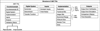
Figure 2. Structure of the .MAT file for representing counterexamples.

The attributes are defined in the .MAT file with the following structure: counterexample that represents the counterexample identification; digital system that represents the numerator, denominator, and transfer function representation; inputs that represent the input vector and initial states; implementation that represents the integer and fractional bits, dynamical ranges, delta operator, sample time, bound, and realization form; outputs report the verification and simulation results, execution time in MATLAB, and comparison status, where it reports whether the counterexample is reproducible or not. Importantly, all execution times are actually CPU times, i.e., only the elapsed time periods spent in the allocated CPUs, which is measured with the times system call (POSIX system).

3.5. DSValidator Usage

DSValidator can be called via command line in MATLAB as:

validation(path, property, ovmode, rmode, filename)

where path is the directory with all counterexamples; property is defined as: “m” for minimum phase; “s” for stability; “o” for overflow; and “lc” for limit cycle; ovmode represents the overflow mode: “wrap” for wrap-around mode (default) and “saturate” for saturation mode; rmode represents the rounding mode, which can be “round” (default) and “floor”; filename represents the .MAT filename, which is generated after the validation process; by default, the .MAT file is named as digital_system. After executing the validation command, DSValidator prints statistics about the counterexamples validation. Fig. 3 shows a report about the digital system represented in Eq. (3) for realizations DFI, DFII, and TDFII.

⬇

1Running Automatic Validation…

2Counterexamples (CE) Validation Report…

3CE 1 time: 0.081929 status: reproducible

4CE 2 time: 0.013996 status: reproducible

5CE 3 time: 0.009488 status: reproducible

6General Report:

7Total Counterexamples Reproducible: 3

8Total Counterexamples Irreproducible: 0

9Total Counterexamples: 3

10Total Execution Time: 0.10541

Figure 3. Counterexample Reproducibility Report.

4. Case Study: Controllers for UAVs

4.1. Benchmarks Description

Here, we evaluated DSValidator for a set of $11$ digital controllers extracted from a real quadrotor unmanned aerial vehicle (UAV) (bouabdallah, ). DSValidator has also been evaluated with other control system benchmarks and experimental results are available online. The experiments for the UAV controllers evaluate overflow, minimum-phase, stability, and limit-cycle in $33$ different numerical formats: $3$ for each digital controller, using $3$ different realizations forms (i.e., DFI, DFII, and TDFII), which resulted in $99$ different verification tasks for each property ($396$ verification tasks in total). The chosen number of bits, associated to each implementation, is based on the impulse response sum proposed by Carletta et al. (carletta, ).

4.2. Experimental Setup

For all evaluated benchmarks, we generated “.out” files that contain the counterexamples and verification results (i.e., successful and failed) produced by DSVerifier (dsverifier, ) allied to two verifiers: CBMC (cbmc, ) and ESBMC (esbmc, ). In addition, the signal input range lies between $-1$ and $1$, that is, the sensor (gyroscope) output bound in normal conditions. Using this configuration, inputs employed during the limit-cycle or overflow verification is limited between $-1$ and $1$. All experiments with DSValidator v$1$.$1$.$0$ were conducted on an otherwise idle Intel Core i$7-2600$ $3.40$ GHz processor, with $24$ GB of RAM, running Ubuntu $64$-bits. Additionally, the time presented in Table 1 is related to the average of $20$ executions for each benchmark; the measuring unit is always in seconds based on the CPU time computed in MATLAB; we did not restrict the memory consumption for the experiments.

4.3. Experimental Results

DSVerifier produced $24$ counterexamples for overflow, $27$ for limit-cycle, $54$ for minimum-phase, and $54$ for stability ($159$ counterexamples in total). Table 1 shows the DSValidator results for the quadrotor attitude system digital controllers, where “Property” describes the property that is evaluated by DSValidator, “CE Reproducible” indicates the number of counterexamples that are successfully reproduced, “CE Irreproducible” indicates the number of counterexamples that are not reproducible, and “Time” provides the runtime in seconds for all simulations on each property.

Table 1. Results for the Quadrotor Attitude System.

Property	CE Reproducible	CE Irreproducible	Time
Overflow	24	0	0.190 s
Limit Cycle	26	1	0.483 s
Minimum-Phase	54	0	0.012 s
Stability	54	0	0.188 s

Note that the automated validation of all counterexamples took less than $1$ second. We consider these times short enough to be of practical use to engineers. The present results also show that all counterexamples (except one) generated by the underlying verifier, considering FWL effects and different realizations forms (i.e., DFI, DFII and TDFII), are sound and reliable since DSValidator is able to simulate the underlying digital system in MATLAB, and then reproduce the respective counterexample. However, for the limit cycle property, there is one counterexample that was not reproduced in DSValidator; DSVerifier did not take into account overflow in intermediate operations to compute the system’s output using the DFII realization form; this bug was confirmed and fixed by the DSVerifier’s developer via a github commit.

5. Conclusions

DSValidator can validate counterexamples produced for the quadrotor attitude system digital controllers, taking into account implementation aspects (fixed-point arithmetic and realization), overflow-mode (saturate or wrap-around), and rounding-mode (floor and round), to simulate a given digital system with its respective counterexample in MATLAB. Currently, DSValidator is able to perform counterexample reproducibility for stability, minimum-phase, limit-cycle, and overflow occurrences. Given the current literature in verification, there is no other automated MATLAB toolbox to reproduce digital system counterexamples generated by verifiers, and to show the reason by which a counterexample cannot be reproduced to validate and endorse the employed verification and most importantly to avoid false alarms. As future work, we expect to expand the field of digital system verification with the availability of other verifiers so that DSValidator can be applied to establish trust in untrusted verification results for highly-complex systems.

Appendix: DSValidator Demonstration

Preconditions and Prerequisites

In order to execute DSValidator in MATLAB, user must install the DSValidator tool in the Linux version of MATLAB 2016a. Each counterexample must be stored as a “.out” file extension. If the user has more than one digital system to be validated, a directory with all “.out” files must be created.

Tool required: MATLAB (version: 2016a).

Operating System: Linux (recommended: Ubuntu 16.04 LTS.)

Installing DSValidator:

In order to install DSValidator, user must download the DSValidator installation file from the DSVerifier web page (http://dsverifier.org/wp-content/uploads/2017/06/dsvalidator-matlab-toolbox-v1.1.0.tar.gz). After that, the following steps must be executed:

1. Open MATLAB and select the folder where you have extracted the DSValidator tar.gz file.

2. Execute the file with the “$.mltbx$” extension (or double-click on it); a pop-up screen to install DSValidator will be shown.

3. Click on the “$install$” button. After installing DSValidator, another pop-up screen will be shown to indicate that DSValidator has been successfully installed in MATLAB.

User should visualize DSValidator installed in the $toolbox\leavevmode\nobreak\ menu$ located at the MATLAB toolbar.

Installing DSVerifier:

In order to install DSVerifier, user must download and extract the DSVerifier installation file from http://dsverifier.org/wp-content/uploads/2017/03/dsverifier-v2.0.3-esbmc-v4.0-cbmc-5.6.tar.gz.

1. Before using DSVerifier, an environment variable called DSVERIFIER_HOME must be configured. The user should add it to the .bashrc file as follows:

   export DSVERIFIER_HOME=’path to dsverifier folder’

2. After setting the environment variable, the following command-line should be used to update the respective variables:

   source .bashrc

3. User should download the (desired) version of CBMC or ESBMC executables for DSVerifier. This package contains CBMC v5.6 and ESBMC v4.0, which should be added to

   DSVERIFIER_HOME/model-checker

4. User needs to install the Eigen library (e.g., eigen3, eigen3-static, and eigen3-devel depending on the distribution) and GCC version 5.4 (or higher) if he/she wants to compile the DSVerifier source code for another operating system.

Preparing the “.out” file with the counterexample

In DSVerifier, users must provide a specification that contains the digital-system numerator and denominator coefficients; the implementation specification that contains the number of bits in the integer and fractional parts; and the input range. For delta realizations, user must also provide the delta operator. In the command-line version, DSVerifier can be invoked as:

dsverifier <file> --realization <i> --property <j>
--x-size <k> --BMC <bmc> --show-ce-data > file.out

where <file> is the digital-system specification file, <i> is the chosen realization form, <j> is the property to be verified, <k> is the verification bound, i.e., the number of times that the digital system is unwound, while the parameter <bmc> indicates the BMC tool to be used (CBMC or ESBMC).

For an ANSI-C specification file with many controllers (or filters), additional macro parameters must be provided (DDS$\_$ID and DIMPLEMENTATION$\_$ID):

dsverifier <file> --realization <i> --property <j>
--x-size <k>      --BMC <bmc> -DDS$\_$ID=<l>
-DIMPLEMENTATION$\_$ID=<m> --show-ce-data      > file.out

where <file> is the digital-system specification file, <i> is the chosen realization form, <j> is the property to be verified, <k> is the verification bound, <bmc> is the BMC tool to be used (CBMC or ESBMC), <l> is the digital controller $id$ in the specification file, and <m> represents the digital controller implementation.

Currently, $3$ realization forms are supported for digital controllers: direct form I (DFI), direct form II (DFII), and transposed direct form II (TDFII). Additionally, we support delta realizations to check stability and minimum-phase, i.e., delta direct form I (DDFI), delta direct form II (DDFII), and transposed delta direct form II (TDDFII). We also support $4$ different properties to validate the counterexample: overflow, limit cycle, stability, and minimum-phase. Fig. 4 shows an ANSI-C specification file with $1$ controller and $2$ implementations:

⬇

1#include <dsverifier.h>

2#if DS_ID == 1

3 digital_system ds = {

4 .b = { 1.5, -0.5 },

5 .b_size = 2,

6 .a = { 1.0, 0.0 },

7 .a_size = 2,

8 .sample_time = 0.02

9 };

10 #define IMPLEMENTATION_COUNT 2

11 #if IMPLEMENTATION_ID == 1

12 implementation impl = {

13 .int_bits = 2,

14 .frac_bits = 14,

15 .max = 1.0,

16 .min = -1.0,

17 };

18 #endif

19 #if IMPLEMENTATION_ID == 2

20 implementation impl = {

21 .int_bits = 4,

22 .frac_bits = 12,

23 .max = 1.0,

24 .min = -1.0,

25 };

26 #endif

27#endif

Figure 4. A digital controller specification file used by DSVerifier.

Using the specification shown in Fig. 4 as an input.c file, DSVerifier can be invoked to check a specific property. The parameter --show-ce-data must be appended to DSVerifier to ensure that the counterexample is provided in a “.out” file. In our particular example, the goal is to check for an overflow violation, that considers the digital controller for DFI and DFII realizations, and $2$ different numerical formats (<2,14> and <4,14>). DSVerifer can be invoked as:

dsverifier input.c --realization DFI --property OVERFLOW --x-size 10 --BMC CBMC -DDS$\_$ID=1 -DIMPLEMENTATION$\_$ID=1 --show-ce-data
> ds1$\_$impl1$\_$DFI.out

To verify the same digital controller, but with the second implementation (<4,14>) and DFI realization:

dsverifier input.c --realization DFI --property OVERFLOW --x-size 10 --BMC CBMC -DDS$\_$ID=1 -DIMPLEMENTATION$\_$ID=2 --show-ce-data
> ds1$\_$impl2$\_$DFI.out

Using DFII realization to check for an overflow violation in the first implementation <2,14>:

dsverifier input.c --realization DFII --property OVERFLOW --x-size 10 --BMC CBMC -DDS$\_$ID=1 -DIMPLEMENTATION$\_$ID=1 --show-ce-data
> ds1$\_$impl1$\_$DFII.out

Last, for the second implementation (<4,12>) using DFII realization:

dsverifier input.c --realization DFII --property OVERFLOW --x-size 10 --BMC CBMC -DDS$\_$ID=1 -DIMPLEMENTATION$\_$ID=2 --show-ce-data
> ds1$\_$impl2$\_$DFII.out

Now, we have $4$ output files that are generated with the respective counterexample for the overflow property, as follows:

ds1$\_$impl1$\_$DFI.out, ds1$\_$impl2$\_$DFI.out, ds1$\_$impl1$\_$DFII.out, ds1$\_$impl2$\_$DFII.out

If we open a “.out” file (e.g., ds1$\_$impl1$\_$DFI.out), then we visualize the counterexample shown in Fig. 5.

⬇

1VERIFICATION FAILED

2Counterexample Data:

3 Property = OVERFLOW

4 Numerator = { 0.1, -0.09996 }

5 Denominator = { 1.0, -1.0 }

6 X Size = 10

7 Sample Time = 0.02

8 Implementation = <10,6>

9 Numerator (fixed-point) = { 384.0, -128.0 }

10 Denominator (fixed-point) = { 256.0, 0.0 }

11 Realization = DFI

12 Dynamic Range = {-1,1}

13 Inputs = { 85.328125, -0.0625, 0.0, -128.6875, -215.984375, -256.0, 256.0, -197.359375, 0.0 85.34375 }

14 Outputs = { 128.0, -42.765625, 0.03125, -193.03125, -259.640625, -276.0, 512.0, -424.046875, 98.6875, 128.015625 }

Figure 5. Counterexample for ds1$\_$impl1$\_$DFI.out generated by DSVerifier.

Running DSValidator

After verifying a given digital-system, one (or more) .out file(s) is (are) generated, which must be saved in a directory, e.g., “/overflow”. In order to check whether a given counterexample is reproducible and reliable, user must invoke DSValidator in the MATLAB command-line as follows:

validation(’/overflow’, ’o’, ’’, ’’, ’ds_overflow’)

Considering the test cases ds1$\_$impl1$\_$DFI.out and
ds1$\_$impl1$\_$DFII.out, the validation output has the following report as shown in Fig. 6.

⬇

1Counterexamples (CE) Validation Report…

2CE 1 time: 0.08845 status: reproducible

3CE 2 time: 0.010247 status: reproducible

4General Report:

5Total Counterexamples Reproducible: 2

6Total Counterexamples Irreproducible: 0

7Total Counterexamples: 2

8Total Time Execution: 0.098697

Figure 6. Automated Counterexample Validation Report by DSValidator.

A ds_overflow.mat file is created with $2$ records; the first one is related to ds1$\_$impl1$\_$DFI.out, while the second one is related to ds1$\_$impl1$\_$DFII.out.

Analyzing the DSValidator Report

Fig. 6 shows the report related to the validation process of $2$ test cases; note that in this report, there are $3$ important pieces of information: “test case $id$”, “execution time”, and “validation status”. The “test case $id$” represents the test case identification that is validated; “execution time” reports in seconds the time to reproduce the test case in MATLAB; “validation status” reports successful or failed; successful means that the counterexample produced by DSVerifier is reproducible, while failed means that there is a divergence about the results between MATLAB and DSVerifier. At the end of the validation report, the total number of successful and failed test cases is provided as well as the total execution time spent during the simulation.

After the validation process, we can individually check other functions in DSValidator to inspect a specific step or process. For instance, if we want to inspect the overflow graphic representation (see Fig. 7), then we can invoke the function plot_overflow(system) as follows:

plot_overflow(ds_overflow(1))

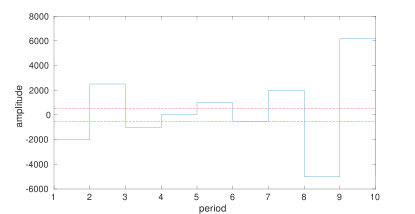
Figure 7. Overflow Detection Graphic.

If we want to visualize the limit cycle graphic representation (see Fig. 8), then we can invoke the function plot_limit_cycle(system) as follows:

plot_limit_cycle(ds_system)

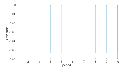
Figure 8. Limit Cycle Detection Graphic.

Other functions from DSValidator can be used to check the counterexamples, e.g., there are functions to reproduce the rounding mode, quantization process, and fixed-point operations. Consider the digital system represented by Eq. (4):

(4) $$H(z)=\frac{0.1+z^{3}-0.3z^{2}+0.3{z}-0.1}{z^{3}+1.8z^{2}+1.14z+0.272}.$$

If we want to check FWL effects on poles and zeros, we must call:

plot_zero_pole(ds_system).

Fig. 9 shows the poles and zeros graphic representation with (and without) FWL effects. Note that when we consider FWL effects in Fig. 9, one zero is out of the $z$-plane unitary circle and thus the controller is a non-minimum-phase system.

We can simulate stability or minimum-phase using the following commands:

simulate_stability(ds_system)

simulate_minimum_phase(ds_system)

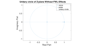
(a) Poles and Zeros Graphic without FWL Effects

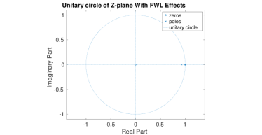
(b) Poles and Zeros Graphic with FWL Effects

Figure 9. Poles and Zeros Graphic with and without FWL Effects.

As a result, those functions return successful or failed. If we execute the example for the digital system represented by Eq. (4), the result for stability is successful, which means that the system is stable. The minimum-phase result is failed, which means that the controller is a non-minimum-phase system.

Another very useful function in DSValidator is the fwl function that obtains the FWL format of a polynomial, considering implementation aspects. This particular function can be called as:

fwl(poly,l)

where poly represents the polynomial and l represents the fractional bits implementation. Considering Eq. (5) as a denominator from a digital system

(5) $$A(z)=z^{3}+1.8z^{2}+1.14z+0.272,$$

and applying the function fwl in A(z) using $13$ fractional bits, the results is:

>> fwl([1 1.8 1.14 0.272],13)

>> 1.0000 1.7999 1.1399 0.2720

The screencast is available at https://www.youtube.com/playlist?list=PL_Vp1B_NN0gC1-nZtHGHDI2jIN6WvY_6e

References

- (1) Diniz P., da Silva E., Netto S. (2010) “Digital Signal Processing: System Analysis and Design”. E-Libro, Cambridge University Press
- (2) Bessa, I. V., Ismail, H. I., Cordeiro, L. C., Chaves Filho, J. E.(2016) “Verification of fixed-point digital controllers using direct and delta forms realizations.” Design Autom. for Emb. Sys., 20(2): pp. 95–126.
- (3) S. Fadali and A. Visioli (2009) “Digital Control Engineering: Analysis and Design.” ser. Electronics & Electrical, Elsevier/Academic Press, vol. 303.
- (4) R. Istepanian and J. Whidborne (2001) “Digital Controller Implementation and Fragility: A Modern Perspective”, ser. Advances in Industrial Control, Springer London.
- (5) Bessa, I. V., Ismail, H. I., Palhares, R., Cordeiro, L. C., Chaves Filho, J. E. (2017) “Formal non-fragile stability verification of digital control systems with uncertainty”. IEEE Trans. Computers, 66(3): pp. 545–552.
- (6) Monteiro, F. (2016) “Bounded Model Checking of State-Space Digital Systems: The Impact of Finite Word-Length Effects on the Implementation of Fixed-Point Digital Controllers Based on State-Space Modeling”. In FSE, pp. 1151–1153.
- (7) Ismail, H. I., Bessa, I. V., Cordeiro, L. C., Chaves Filho, J. E., Lima Filho, E. B. (2015) “DSVerifier: A Bounded Model Checking Tool for Digital Systems”. In SPIN, LNCS 9232, pp. 126–131.
- (8) Cordeiro, L. C., Fischer, B., Marques-Silva, J. P.(2012) “SMT-Based Bounded Model Checking for Embedded ANSI-C Software,” TSE vol. 38 (4), pp. 957–974.
- (9) Kroening, D. and Tautschnig, M. (2014) “CBMC – C Bounded Model Checker,” In TACAS, LNCS 8413, pp. 389–391.
- (10) Abreu, R. B., Gadelha, M. Y. R., Cordeiro, L. C., Lima Filho, E. B., Silva Jr., W. S. (2016) “Bounded Model Checking for Fixed-Point Digital Filters”. Journal of The Brazilian Computer Society, v.20(1), pp. 1–20.
- (11) Matlab Toolbox (2017). In https://www.mathworks.com/products/.
- (12) Beyer, D., Dangl, M., Dietsch, D., Heizmann, M., Stahlbauer, A. (2015) “Witness validation and stepwise testification across software verifiers”. In FSE, pp. 721–733.
- (13) Beyer, D. and Keremoglu, M. (2011) “CPAchecker: A Tool for Configurable Software Verification”. In CAV, LNCS, 6806, pp. 184–190.
- (14) Heizmann, M., Dietsch, D., Leike, J., Musa, B., and Podelski, A. (2015) “Ultimate Automizer with array interpolation”. In TACAS, LNCS 9035, pp. 455–457.
- (15) Bouabdallah S. (2007) “Design and control of quadrotors with application to autonomous flying”. Ph.D. dissertation, École Polytechnique Fédérale de Lausanne.
- (16) Bauer, P. H., Leclerc, L. (1991) “A computer-aided test for the absence of limit cycles in fixed-point digital filters”. In IEEE Trans. Signal Processing, 39(11): pp. 2400–2410.
- (17) Premaratne, K., Kulasekere, E. C., Bauer, P.H, and Leclerc, L. (1996) “An exhaustive search algorithm for checking limit cycle behavior of digital filters”. In IEEE Trans. Signal Processing, 44(10): pp. 2405–2411.
- (18) Chaves, L., Bessa, I. V., Kroening, D., Cordeiro, L., and Filho, E. B.(2017) “Verifying Digital Systems with MATLAB”. In ISSTA, 2017 (to appear).
- (19) Carletta, J., Veillette, R., Krach, F., and Fang, Z. (2003) “Determining appropriate precisions for signals in fixed-point IIR filters”. In Design Automation Conference, pp. 656–661, Anaheim, CA, USA.