HU-EP 16/36
KW 16-003
30 years, some 700 integrals, and 1 dessert
                               or:
Electroweak two-loop corrections to the $Z{\bar{b}}b$ vertex

Abstract:

The one-loop corrections to the weak mixing angle $\sin^{2}\theta_{\rm eff}^{\rm b}$, derived from the $Z{\bar{b}}b$ vertex, are known since 1985. It took another 30 years to calculate the complete electroweak two-loop corrections to $\sin^{2}\theta_{\rm eff}^{\rm b}$. The main obstacle was the calculation of the ${\cal O}(700)$ bosonic two-loop vertex integrals with up to three mass scales, at $s=M_{Z}^{2}$. We did not perform the usual integral reduction and master evaluation, but chose a completely numerical approach, using two different calculational chains. One method relies on publicly available sector decomposition implementations. Further, we derived Mellin-Barnes (MB) representations, exploring the publicly available MB suite. We had to supplement the MB suite by two new packages: AMBRE 3, a Mathematica program, for the efficient treatment of non-planar integrals and MBnumerics for advanced numerics in the Minkowskian space-time. Our preliminary result for LL2016, the “dessert”, for the electroweak bosonic two-loop contributions to $\sin^{2}\theta_{\rm eff}^{\rm b}$ is:
     $\Delta\sin^{2}\theta_{\rm eff}^{\rm b(\alpha^{2},\rm bos)}=\sin^{2}\theta_{W}~{}\Delta\kappa_{\mathrm{b}}^{(\alpha^{2},\rm bos)}$, with $\Delta\kappa_{\mathrm{b}}^{(\alpha^{2},\rm bos)}=-1.0276\times 10^{-4}$.
This contribution is about a quarter of the corresponding fermionic corrections and of about the same magnitude as several of the known higher-order QCD corrections. The $\sin^{2}\theta_{\rm eff}^{\rm b}$ is now predicited in the Standard Model with a relative error of $10^{-4}$ [1].

Preface

Der Wahnsinn
ist nur eine schmale Brücke
die Ufer sind Vernunft und Trieb

Rammstein, http://www.magistrix.de/lyrics/Rammstein/Du-Riechst-So-Gut-26274.html

LL2016 in Leipzig was the 13^th edition, and it was my last Loops and Legs conference as an organizer, and perhaps also as a participant. I founded it, together with Johannes Blümlein and Martina Mende, in April 1992 as a bi-annual event; it was a follow-up of the 1989 November changes in Germany. The aim was an overview of the recent developments in perturbative quantum field theory with focus on applications to precision collider experiments. We attempted a mix of all the relevant research directions, but also a mix of both younger and more experienced collegues. From time to time we had to invent some modernizations like parallel sessions or online proceedings. In the early years the focus was more at direct phenomenological applications, and now it is more on advanced technical developments. The steady high scientific level has been guaranteed by the participants, and the discussions were top-level, lively and sometimes even hot.

My own research reflects the above observations. Since 1977, I am engaged in complete electroweak radiative corrections for collider physics. A statement by a head of an institute: “For me you are one who calculates integrals.” My most successful project is ZFITTER (with Dima Bardin et al., see http://sanc.jinr.ru/users/zfitter). ZFITTER became the standard software for the study of the Z boson resonance at LEP and elsewhere, and it was used to predict the masses of the top quark and the Higgs boson prior to their discoveries. Many PhD students used it. Recently, ZFITTER even got illegally copied by non-experts in order to promote their carriers. In 1985, we calculated the one-loop corrections to $Z\to{\bar{b}}b$. The corresponding FORTRAN code ZRATE, later ZWRATE and ROKANC, became the center of the Standard Model library of ZFITTER. 30 years later, at this year’s Loops and Legs conference, I presented an electroweak Standard Model two-loop calculation for $Z\to{\bar{b}}b$, performed together with my coauthors. This project started in 2012 at a meeting at the Max-Planck Institute in Munich, where I met Ayres Freitas. At that meeting the second-oldest speaker was about 20 years younger than me … Our numerical fitting formula for the $Z{\bar{b}}b$ weak mixing angle will, presumably, get included into software packages like ZFITTER. During work on this report on the $Z{\bar{b}}b$ project I understood that there is a deep connection to one of my other hobbies – the S-matrix approach to the $Z$ resonance. This connection will be described shortly in the introduction, although it was not part of the oral presentation at the conference. Its understanding certainly will help to create a strict one per mille analysis tool for the $Z$ resonance as it is assumed to be needed for the next $e^{+}e^{-}$ collider, and perhaps at the LHC.

I would like to thank my collegues for a decade-long, competitive, but also collaborative work in the research field of elementary particle physics, notably Arif Akhundov, Dima Bardin, Penka Christova, Dietmar Ebert, Jochem Fleischer, Ayres Freitas, Janusz Gluza, Wolfgang Hollik, Lida Kalinovskaya, Max Klein, Arnd Leike, Gottfried Mann, Sven Moch, Sabine Riemann, as well as Frank Kaschluhn, Karl Lanius and Paul Söding for support. With my PhD students Dietrich, Mark, Jochen, Alejandro, Valery (see https://www.genealogy.math.ndsu.nodak.edu/id.php?id=29907), and now Johann and Ievgen, work was and is pleasure. In February 2015 I underwent a medical surgery, and I thank Professor Dr. med. habil. Ahmed Magheli from Charite in Berlin that I could afterwards continue working and successfully apply as a Fellow of the Polish Alexander von Humboldt Research Scholarship 2015, with host Janusz Gluza at the Silesian University at Katowice.

Tord Riemann, 21 October 2016

1 Introduction

The study of the $Z$ boson resonance in $e^{+}e^{-}$ annihilation,

$$e^{+}e^{-}\to(\gamma,Z)\to f^{+}f^{-}~{}(+~{}n\gamma),$$ (1)

has been performed with high precision at LEP and is planned with better precision at future $e^{+}e^{-}$ colliders. Correspondingly, the theoretical predictions in the Standard Model are needed with 2-loop accuracy in the weak sector, and even better for QED and QCD. Usually, the theoretical analysis is based not on cross sections as measured in reaction (1), including non-observed additional photons (and gluons), but on so-called pseudo-observables, corresponding to

$$e^{+}e^{-}\to(\gamma,Z)\to f^{+}f^{-},$$ (2)

or even to the simpler reaction

$$Z\to f^{+}f^{-}~{}(+~{}n\gamma).$$ (3)

This is quite similar to the analysis of LHC events, which one tries to focus on the underlying hard $2\to 2$ process. As a result, the analysis of observables rests on two relatively independent steps:

• Unfolding the observed cross sections and representing them as $2\to 2$ (pseudo-) observables; the theoretical frame has to be sufficiently general in order not to bias step 2.

• Confronting the pseudo observables with specific theory predictions.

A key element of the theoretical analysis is the $Z{\bar{b}}b$ vertex, whose prediction at two electroweak loops is the subject of our study. Two pseudo-observables are related to this vertex:

• The partial decay width $\Gamma(Z\to{\bar{b}}b)$.

• The decay asymmetry, related to the parameter $A_{b}$; we give its definition below in (9).

The partial decay width $\Gamma(Z\to{\bar{b}}b)$ is related to the peak cross-section $\sigma_{T}$ of $e^{+}e^{-}\to(\gamma,Z)\to b^{+}b^{-}(+n\gamma)$, also to the pseudo-cross section of $e^{+}e^{-}\to(\gamma,Z)\to b^{+}b^{-}$, and $A_{b}$ is related to the angular asymmetry of the cross-sections.

In Born approximation everything looks relatively easy. Neglecting here photon exchange, and using a Breit-Wigner resonance $Z$ propagator with a priori mass $M_{Z}$ and width $\Gamma_{Z}$ of the $Z$ boson, one derives a qualitatively good description of the $Z$ line shape close to the peak:

$$\frac{d\sigma^{B}}{d\cos\theta} \sim G_{F}^{2}~{}\left|\frac{s}{s-M_{Z}^{2}+iM_{Z}{\color[rgb]{0,0,0}\Gamma_{Z}}}\right|^{2}$$

$$\times~{}\left[(a_{e}^{B\;2}+v_{e}^{B\;2})(a_{b}^{B\;2}+v_{b}^{B\;2})(1+\cos^{2}\theta)+(2a_{e}^{B}v_{e}^{B})(2a_{b}^{B}v_{b}^{B})(2\cos\theta)\right].$$

Symmetric or anti-symmetric integration over $\cos\theta$ allows to determine the two independent contributions. One of them is the total cross section,

$$\sigma_{T}^{B} \equiv \int_{-1}^{1}d\cos\theta\frac{d\sigma^{B}}{d\cos\theta}\sim\left|\frac{s}{s-M_{Z}^{2}+iM_{Z}{\color[rgb]{0,0,0}\Gamma_{Z}}}\right|^{2}G_{F}^{2}\left(a_{e}^{B\;2}+v_{e}^{B\;2}\right)\color[rgb]{0,0,0}{\left(a_{b}^{B\;2}+v_{b}^{B\;2}\right)}\sim{\Gamma_{e}^{B}}\Gamma_{b}^{B},$$ (5)

and the other one the forward-backward asymmetry,

$$\sigma_{FB}^{B} \equiv \left[\int_{0}^{1}-\int_{-1}^{0}\right]d\cos\theta\frac{d\sigma^{B}}{d\cos\theta}\sim\left|\frac{s}{s-M_{Z}^{2}+iM_{Z}{\color[rgb]{0,0,0}\Gamma_{Z}}}\right|^{2}G_{F}^{2}(2a_{e}^{B}v_{e}^{B})~{}(2a_{b}^{B}v_{b}^{B}),$$ (6)

$$A_{FB}^{B} \equiv \frac{\sigma_{FB}^{B}}{\sigma_{T}^{B}}=\frac{3}{4}~{}\frac{2a_{e}^{B}v_{e}^{B}}{a_{e}^{B\;2}+v_{e}^{B\;2}}~{}\color[rgb]{0,0,0}{\frac{2a_{b}^{B}v_{b}^{B}}{a_{b}^{B\;2}+v_{b}^{B\;2}}}\equiv\frac{3}{4}~{}{A_{e}^{B}}~{}{A_{b}^{B}}.$$ (7)

We observe the factorization of $\sigma_{T}^{B}$ into the product of two partial widths,

$$\Gamma_{f}^{B}=\frac{G_{F}M_{Z}^{3}}{\sqrt{2}~{}6\pi}c_{f}\left(a_{f}^{B\;2}+v_{f}^{B\;2}\right),$$ (8)

and of $A_{FB}^{B}$ into the product of two asymmetry functions,

$$A_{f}^{B}=\frac{2a_{f}^{B}v_{f}^{B}}{a_{f}^{B\;2}+v_{f}^{B\;2}}.$$ (9)

In Born approximation it is $a_{f}^{B}=\pm\frac{1}{2}$, $Q_{e}=-1$, $c_{f}$ the color factor, and

$$\frac{v_{f}^{B}}{a_{f}^{B}}=1-4|Q_{f}|\sin^{2}\theta_{W}.$$ (10)

The vector and axial vector couplings will get loop corrections, which may be calculated from the vertex diagrams ${\bf V}^{Zf\bar{f}}_{\mu}(k^{2})$; for the $Z{\bar{b}}b$-vertex:

$$g_{\rm V}^{b}(k^{2})|_{k^{2}=M_{Z}^{2}} = \frac{1}{2(2-D)k^{2}}\,{\rm Tr}[\gamma^{\mu}\,\cancel{p}_{1}\,{\color[rgb]{0,0,0}{\bf V}^{Zb\bar{b}}_{\mu}}\,\cancel{p}_{2}]|_{k^{2}=M_{Z}^{2}},$$ (11)

$$g_{\rm A}^{b}(k^{2})_{k^{2}=M_{Z}^{2}} = \frac{1}{2(2-D)k^{2}}\,{\rm Tr}[\gamma_{5}\,\gamma^{\mu}\,\cancel{p}_{1}\,{\color[rgb]{0,0,0}{\bf V}^{Zb\bar{b}}_{\mu}}\,\cancel{p}_{2}]_{k^{2}=M_{Z}^{2}}.$$ (12)

Here, we relate vertex corrections to effective couplings. In reality, realistic cross sections are measured, and one has to relate their couplings to $g_{\rm V}^{b}(k^{2})$ and $g_{\rm A}^{b}(k^{2})$.

Fitting programs like Gfitter are relating “experimental” values of e.g. $\Gamma_{b}$, $A_{b}$ with their theoretical predictions, e.g. in the standard model [2]. But does this fit the original pseudo-observables? To some approximation, it does, as can be seen in the Born formulae. But one has to control the quantum corrections safely. We know since long how to relate pseudo-observables in a strict way to the loop corrections [3, 4, 5, 6, 7]. The amplitude for $e^{+}e^{-}$ annihilation into two massless fermions, and we assume here the final state to be massless, may be described to all orders of perturbation theory by four complex-valued form factors, which depend on the masses and the invariants $s$ and $t$, and which are chosen here to be $\rho_{ef},\kappa_{e},\kappa_{f},\kappa_{ef}$; we quote from [6], eq. (3.3.1):

$${\cal A}^{\scriptscriptstyle{eff}}_{\scriptscriptstyle{Z}}(s,t) \sim i\,e^{2}\,4\,I^{(3)}_{e}I^{(3)}_{f}\frac{\chi_{Z}(s)}{s}{\rho_{ef}(s,t)}\biggl{\{}\gamma_{\mu}{\left(1+\gamma_{5}\right)}\otimes\gamma_{\mu}{\left(1+\gamma_{5}\right)}$$

$$-4|Q_{e}|s^{2}_{\scriptscriptstyle{W}}{\kappa_{e}(s,t)}\gamma_{\mu}\otimes\gamma_{\mu}{\left(1+\gamma_{5}\right)}-4|Q_{f}|s^{2}_{\scriptscriptstyle{W}}{\kappa_{f}(s,t)}\gamma_{\mu}{\left(1+\gamma_{5}\right)}\otimes\gamma_{\mu}$$

$$+16|Q_{e}Q_{f}|s^{4}_{\scriptscriptstyle{W}}{\kappa_{ef}(s,t)}\gamma_{\mu}\otimes\gamma_{\mu}\biggr{\}}.$$

We use the definitions

$$\chi_{Z}(s) = \frac{G_{F}M_{Z}^{2}}{\sqrt{2}~{}2\pi\alpha}~{}\rho_{Z}(s),$$ (14)

$$\rho_{Z}(s) = \frac{s}{s-M_{Z}^{2}+iM_{Z}{\color[rgb]{0,0,0}\Gamma_{Z}(s)}}.$$ (15)

For the complete amplitude one sums over all relevant diagrams so that the form factors are perturbative series:

$$\rho_{ef} = 1+\delta\rho_{ef}=1+\frac{\alpha}{\pi}\delta\rho_{ef}^{(1)}+\cdots,$$ (16)

$$\kappa_{a} = 1+\delta\kappa_{a}=1+\frac{\alpha}{\pi}\delta\kappa_{a}^{(1)}+\cdots,~{}~{}~{}a=e,f,ef.$$ (17)

Compared to a “naive” notation, we split from the rest of the amplitude the form factor $\rho_{ef}$ multiplicatively. If a diagram is represented by an original set $\{\rho_{ef},{\bar{\kappa}_{e}},{\bar{\kappa}_{f}},{\bar{\kappa}_{ef}}\}$, this yields re-definitions for all the $\kappa_{a}$:

$$\kappa_{a}=\frac{{\bar{\kappa}_{a}}}{\rho_{ef}},~{}~{}~{}a=e,f,ef.$$ (18)

The form factors, if introduced as it is done here, may be used for definitions of an effective Fermi constant and three effective weak mixing angles:

$$G_{F}^{\rm eff} = \rho_{ef}(s,t)~{}G_{F},$$ (19)

$$\sin^{2}\theta_{W,e}^{\rm eff} = \kappa_{e}(s,t)~{}\sin^{2}\theta_{W},$$ (20)

$$\sin^{2}\theta_{W,f}^{\rm eff} = \kappa_{f}(s,t)~{}\sin^{2}\theta_{W},$$ (21)

$$\sin^{2}\theta_{W,ef}^{\rm eff} = \sqrt{\kappa_{ef}(s,t)}~{}\sin^{2}\theta_{W},$$ (22)

where

$$\sin^{2}\theta_{W}\equiv 1-\frac{M_{W}^{2}}{M_{Z}^{2}}.$$ (23)

The unique definition of an effective weak mixing angle is lost.

The Breit-Wigner propagator $\rho_{Z}(s)$ contains a width function which is predicted by perturbation theory. Its calculation deserves special attention, and for the moment the notation $\Gamma_{Z}(s)$ emphasizes that it originates from summing over self-energies like $\Sigma_{Z}(s)$.

The amplitude may be further rewritten, in order to introduce the familiar couplings $v_{f},a_{f}$, which now will cover the loop corrections:

$${\cal A}^{\scriptscriptstyle{eff}}_{\scriptscriptstyle{Z}}(s,t) \sim i\,e^{2}\frac{\chi_{Z}(s)}{s}a_{e}a_{f}{\rho_{ef}(s,t)}\biggl{(}\gamma_{\mu}\gamma_{5}\otimes\gamma_{\mu}\gamma_{5}+\frac{v_{f}}{a_{f}}\gamma_{\mu}\otimes\gamma_{\mu}\gamma_{5}+\frac{v_{e}}{a_{e}}\gamma_{\mu}\gamma_{5}\otimes\gamma_{\mu}+\frac{v_{ef}}{a_{e}a_{f}}\gamma_{\mu}\otimes\gamma_{\mu}\biggr{)}.$$

Here, we made the choice that the axial couplings remain Born like,

$$a_{e} = -\frac{1}{2},$$ (25)

$$a_{f} = \pm\frac{1}{2}.$$ (26)

This choice means that the axial couplings remain to be real constants here, and that the (axial $\times$ axial) radiative corrections coming from a product of two vertices like (12) will be collected in the definition of $\rho_{ef}$,

$$\delta\rho_{ef}^{Z{\bar{e}}eZ{\bar{b}}b} = \frac{g_{\rm A}^{e}(k^{2})_{k^{2}=M_{Z}^{2}}}{a_{e}}~{}\frac{g_{\rm A}^{f}(k^{2})_{k^{2}=M_{Z}^{2}}}{a_{f}},$$ (27)

while the vector couplings are understood to contain radiative corrections. From a final state $Z{\bar{b}}b$ vertex loop correction, one then gets e.g.:

$$v_{e} = v_{e}^{B},$$ (28)

$$v_{b} = v_{e}^{B}+\delta v_{f}^{Z{\bar{b}}b}=v_{e}^{B}+g_{\rm V}^{f}(k^{2})_{k^{2}=M_{Z}^{2}},$$ (29)

$$v_{eb} = v_{e}^{B}\left(v_{b}^{B}+\delta v_{ef}^{Z{\bar{b}}b}\right)=v_{e}^{B}\left(v_{b}^{B}+\delta v_{f}^{Z{\bar{b}}b}\right).$$ (30)

From the above definitions we get three relations between the vector couplings and the form factors $\kappa$:

$$\frac{v_{e}}{a_{e}} = 1-4|Q_{e}|s^{2}_{\scriptscriptstyle{W}}{\kappa_{e}},$$ (31)

$$\frac{v_{f}}{a_{f}} = 1-4|Q_{f}|s^{2}_{\scriptscriptstyle{W}}{\kappa_{f}},$$ (32)

$$\frac{v_{ef}}{a_{e}a_{f}} = \frac{v_{e}v_{f}}{a_{e}a_{f}}+\Delta_{ef},$$ (33)

with

$$\Delta_{ef} = 16|Q_{e}Q_{f}|s_{W}^{4}(\kappa_{ef}-\kappa_{e}\kappa_{f}).$$ (34)

If $\kappa_{ef}-\kappa_{e}\kappa_{f}=0$, there is factorization. Factorization is broken by photonic corrections and by box diagrams, while it is respected by weak vertex corrections and self-energies.

Having defined the amplitude, one may calculate, with standard text book methods, a $2\to 2$ cross section. For unpolarized scattering one gets [4]:

$$\frac{d\sigma^{eff}}{d\cos\theta}=\frac{\pi\alpha^{2}}{2s}|\chi_{Z}(s)|^{2}\left[(1+\cos^{2}\theta)k_{T}+2\cos\theta k_{FB}\right].$$ (35)

The symmetric part depends on

$$k_{T} = |\rho_{ef}|^{2}\left[|a_{e}a_{f}|^{2}+|v_{e}a_{f}|^{2}+|a_{e}v_{f}|^{2}+|v_{ef}|^{2}\right]$$

$$= |\rho_{ef}|^{2}|a_{e}|^{2}|a_{f}|^{2}\left[(1+|\frac{v_{e}}{a_{e}}|^{2})(1+|\frac{v_{f}}{a_{f}}|^{2})+\Delta_{T}\right],$$

with

$$\Delta_{T} = |\Delta_{ef}|^{2}+2\Re e\left(\frac{v_{e}}{a_{e}}\frac{v_{f}}{a_{f}}\Delta_{ef}^{*}\right).$$ (37)

Assuming factorization, this becomes

$$k_{T} = |\rho_{ef}|^{2}\left[(|a_{e}|^{2}+|v_{e}|^{2})(|a_{f}|^{2}+|v_{f}|^{2})\right],$$ (38)

and finally, neglecting additionally the imaginary parts of $v_{e}$ and $v_{f}$ (and of $\Delta_{T}$):

$$k_{T} = |\rho_{ef}|^{2}\left[(a_{e}^{2}+v_{e}^{2})(a_{f}^{2}+v_{f}^{2})\right].$$ (39)

This is the formula usually applied to analyses.

Similarly, for the anti-symmetric cross section part:

$$k_{FB} = |\rho_{ef}|^{2}a_{e}a_{f}\Re e(v_{e}v_{f}^{*}+v_{ef})$$

$$= a_{e}a_{f}\left(2\Re e\left[\frac{v_{e}}{a_{e}}\right]\,2\Re e\left[\frac{v_{f}}{a_{f}}\right]+\Delta_{FB}\right),$$

with

$$\Delta_{FB} = 2\Re e\Delta_{ef},$$ (41)

and after again neglecting non-factorizing terms and imaginary parts:

$$k_{FB} = 2|\rho_{ef}|^{2}(2a_{e}v_{e})~{}(2a_{f}v_{f}).$$ (42)

The cross section formula (35) is the exact result from the amplitude square and averaging over the initial final helicity states.

Here, a technical remark is at the place: Already in Born approximation, the photon exchange leads to non-factorization. It is numerically not small and has to be taken into account. One may, formally, assume that the photon exchange Born amplitude is contained in the above-introduced four form factors. This was exemplified in [8]. Conventionally, one works with two interfering amplitudes as it is described in detail in the publications describing the ZFITTER project [9, 4, 5, 6, 7].

Under the assumption that the form factors are independent of the scattering angle, we get for the total cross section and the forward-backward asymmetry:

$$\sigma_{T} = \frac{4\pi\alpha^{2}}{3s}|\chi_{Z}|^{2}~{}k_{T},$$ (43)

$$\sigma_{FB} = \frac{\pi\alpha^{2}}{s}|\chi_{Z}|^{2}~{}k_{FB},$$ (44)

and the forward-backward asymmetry becomes

$$A_{FB}^{eff} = \frac{3}{4}~{}\frac{k_{FB}}{k_{T}}.$$ (45)

If the form factors depend on the scattering angles, as it is the case for corrections from box diagrams, one has to study the numerical effect of that.

Further observables may be introduced for polarized scattering, where the amplitude (1) is taken between helicity projected states. This may be easily investigated following [4].

The loop-corrected asymmetry parameter $A_{b}$ as defined in (9) will be set in relation to loop-corrected pseudo-observables at $s=M_{\mathrm{Z}}^{2}$, in terms of the angular integrals $\sigma_{FB},\sigma_{T}$ as defined in (1) and (1):

$$A_{FB}^{{\bar{b}}b} = \frac{\sigma_{FB}}{\sigma_{T}}$$

$$= \frac{3}{4}~{}\frac{\Re e[2a_{e}v_{e}~{}2a_{b}v_{b}+4\sin^{2}\theta_{W}|Q_{e}Q_{b}|^{2}(\kappa_{eb}-\kappa_{e}\kappa_{b})]}{|a_{e}a_{b}|^{2}+|v_{e}a_{b}|^{2}+|a_{e}v_{b}|^{2}+|v_{eb}|^{2}}~{}~{}+\textrm{~{}~{} corrections}$$

$$= \frac{3}{4}~{}A_{\mathrm{e}}~{}A_{\mathrm{b}}~{}~{}+\textrm{~{}~{} corrections}.$$

The first “corrections” are due to neglected angular dependences of the form factors, and the second “corrections” are due to neglected non-factorizations and imaginary parts.

As discussed in detail in [10], as well as in earlier work [11, 12], the weak mixing angle $\sin^{2}\theta_{\rm eff}^{\rm b}$ and $A_{\mathrm{b}}$ are determined from the residue $R$ of the leading part of the resonance matrix element ${\cal\bar{M}}$ (48). This residue may be determined in a very good and controlled approximation from the renormalized vector and axial vector couplings of the vertices $V^{Ze\bar{e}}_{\mu}$ and $V^{Zb\bar{b}}_{\mu}$. To do so, we have to understand how the form factors are composed. Besides the terms from $s$ channel $Z$ boson exchange, they contain terms from $s$ channel photon exchange, from box diagrams (with weak bosons, but also with photon exchanges), vertices, self-energies. Some of these terms are enhanced by the resonance form of the transition, others are not. One has to understand some summation of terms which otherwise would explode at $s=M_{Z}^{2}$.

We will now discuss shortly the consequences of the fact that we are studying a resonance. Here arises the question, what is the correct and model-independent formulation of the amplitude from the point of view of general quantum field theory? In order to respect general principles – unitarity, analyticity, gauge invariance – one may use the pole scheme [11]. In the pole scheme, one makes the following ansatz for the amplitude ${\cal\bar{M}}$ as a function of the scattering energy, or as a function of the corresponding relativistic invariant $s$. In a sufficiently small neighborhood around the pole position, it is a Laurent expansion with position of the pole $s_{0}$ defined by the mass $m_{Z}$ and its width $g_{Z}$,

$$s_{0} = m_{Z}^{2}-im_{Z}g_{Z},$$ (47)

and the residue $R$, plus a background term $B$. The latter is a Taylor expansion:

$${\cal\bar{M}}\sim\frac{R}{s-m_{Z}^{2}+im_{Z}g_{Z}}+\sum_{n=0}^{\infty}\frac{b_{n}}{s_{0}}\left(1-\frac{s}{s_{0}}\right)^{n}.$$ (48)

A kind of master formula for $R$ is equation (12), together with (13), of [10, 12]:

$$R =\begin{aligned} &z_{\mathrm{e}}^{(0)}\,R_{ZZ}\,z_{\mathrm{f}}^{(0)}+\left[\hat{z}_{\mathrm{e}}^{(1)}(M_{\mathrm{Z}}^{2})\,z_{\mathrm{f}}^{(0)}+z_{\mathrm{e}}^{(0)}\,\hat{z}_{\mathrm{f}}^{(1)}(M_{\mathrm{Z}}^{2})\right]\left[1+{\Sigma_{ZZ}^{(1)}}^{\prime}(M_{\mathrm{Z}}^{2})\right]\\ &+\hat{z}_{\mathrm{e}}^{(2)}(M_{\mathrm{Z}}^{2})\,z_{\mathrm{f}}^{(0)}+z_{\mathrm{e}}^{(0)}\,\hat{z}_{\mathrm{f}}^{(2)}(M_{\mathrm{Z}}^{2})+\hat{z}_{\mathrm{e}}^{(1)}(M_{\mathrm{Z}}^{2})\,\hat{z}_{\mathrm{f}}^{(1)}(M_{\mathrm{Z}}^{2})\\ &-iM_{\mathrm{Z}}\Gamma_{\mathrm{Z}}\left[\mbox{$\hat{z}_{\mathrm{e}}^{(1)}$}^{\prime}(M_{\mathrm{Z}}^{2})\,z_{\mathrm{f}}^{(0)}+z_{\mathrm{e}}^{(0)}\,\mbox{$\hat{z}_{\mathrm{f}}^{(1)}$}^{\prime}(M_{\mathrm{Z}}^{2})\right],\end{aligned}$$ (49)

$$R_{ZZ} =\begin{aligned} &1-{\Sigma_{ZZ}^{(1)}}^{\prime}(M_{\mathrm{Z}}^{2})\\ &-{\Sigma_{ZZ}^{(2)}}^{\prime}(M_{\mathrm{Z}}^{2})+\left({\Sigma_{ZZ}^{(1)}}^{\prime}(M_{\mathrm{Z}}^{2})\right)^{2}+iM_{\mathrm{Z}}\Gamma_{\mathrm{Z}}\,{\Sigma_{ZZ}^{(1)}}^{\prime\prime}(M_{\mathrm{Z}}^{2})\\ &-\frac{1}{M_{\mathrm{Z}}^{4}}\left({\Sigma_{\gamma Z}^{(1)}}(M_{\mathrm{Z}}^{2})\right)^{2}+\frac{2}{M_{\mathrm{Z}}^{2}}\,{\Sigma_{\gamma Z}^{(1)}}(M_{\mathrm{Z}}^{2})\,{\Sigma_{\gamma Z}^{(1)}}^{\prime}(M_{\mathrm{Z}}^{2}).\end{aligned}$$ (50)

The $\Sigma_{V_{1}V_{2}},V_{i}=Z,\gamma$ stand for self-energies, and the vertices are defined there as

$$\Gamma[Z_{\mu}f\bar{f}] \equiv z_{{\mathrm{f}},\mu}=i\gamma_{\mu}(v_{\mathrm{f}}+a_{\mathrm{f}}\gamma_{5}),$$ (51)

$$\Gamma[\gamma_{\mu}f\bar{f}] \equiv g_{{\mathrm{f}},\mu}=i\gamma_{\mu}(q_{\mathrm{f}}+p_{\mathrm{f}}\gamma_{5}),$$ (52)

$$\hat{z}_{{\mathrm{f}},\mu}(k^{2}) = i\gamma_{\mu}\left[\hat{v}_{\mathrm{f}}(k^{2})+\hat{a}_{\mathrm{f}}(k^{2})\gamma_{5}\right]$$ (53)

$$\equiv i\gamma_{\mu}\left[v_{\mathrm{f}}(k^{2})+a_{\mathrm{f}}(k^{2})\gamma_{5}\right]-i\gamma_{\mu}\left[q_{\mathrm{f}}(k^{2})+p_{\mathrm{f}}(k^{2})\gamma_{5}\right]\frac{\Sigma_{\gamma Z}(k^{2})}{k^{2}+\Sigma_{\gamma\gamma}(k^{2})}.$$

For details of notations, we refer to [10].

Here, ${\cal\bar{M}}$ stands for the functional form of the amplitude introduced in (11). Within our formalism, one may write in full generality:

$$\rho_{ef} = \frac{R_{r}}{s-s_{0}}+\sum_{n=0}^{\infty}\frac{b_{r,n}}{s_{0}}\left(1-\frac{s}{s_{0}}\right)^{n},$$ (54)

$$\kappa_{e} = \sum_{n=0}^{\infty}\frac{b_{e,n}}{s_{0}}\left(1-\frac{s}{s_{0}}\right)^{n},$$ (55)

$$\kappa_{f} = \sum_{n=0}^{\infty}\frac{b_{f,n}}{s_{0}}\left(1-\frac{s}{s_{0}}\right)^{n},$$ (56)

$$\kappa_{ef} = \sum_{n=0}^{\infty}\frac{b_{ef,n}}{s_{0}}\left(1-\frac{s}{s_{0}}\right)^{n}.$$ (57)

Because $\rho$ is chosen to be an overall factor, it is appropriate to include the resonating part of the amplitude here. From the generic formula (48), one gets all the expressions for $\sigma_{T},A_{FB},A_{LR}$ etc. as explained above [13, 14]. As a result, all these quantities $\sigma_{A}$ have the same form, but depend on different terms $R_{A,r}$ and $b_{A,f,n}$, which are bi-linear compositions of the coefficients $R_{r}$ and $b_{f,n}$.

The Breit-Wigner function used here deviates from the Breit-Wigner function as it was used by the LEP collaborations, where $\Gamma_{Z}(s)=s/M_{Z}^{2}~{}\Gamma_{Z}$ was used instead of $\Gamma_{Z}(s)=g_{Z}$. The difference is not negligible and amounts to [15]:

$$m_{Z} = \frac{M_{Z}}{\sqrt{1+\Gamma_{Z}^{2}/M_{Z}^{2}}}~{}\approx~{}M_{Z}-\frac{1}{2}\Gamma_{Z}^{2}/M_{Z}~{}\approx~{}M_{Z}-34~{}\mathrm{MeV},$$ (58)

$$g_{Z} = \frac{\Gamma_{Z}}{\sqrt{1+\Gamma_{Z}^{2}/M_{Z}^{2}}}~{}\approx~{}\Gamma_{Z}-\frac{1}{2}\Gamma_{Z}^{3}/M_{Z}^{2}~{}\approx~{}\Gamma_{Z}-1~{}\mathrm{MeV}.$$ (59)

We have expansions both around the pole position $s_{0}$ and in the coupling constants $\alpha$ and $\alpha_{s}$, and have to assume that $\alpha,\alpha_{s}$ and $g_{Z}/m_{Z}$ and also $1-s/m_{Z}^{2}$ are of the same numerical order. As a consequence, in an electroweak calculation, $R$ is needed to order ${\cal O}(\alpha^{2})$, the coefficients $b_{0}$ to order ${\cal O}(\alpha)$, and the $b_{1}$ etc. to leading order only. One has to observe that also the quantity $g_{Z}$ itself is a prediction of the theory, beginning at order ${\cal O}(\alpha^{2})$.

A further complication comes from the fact that there are not so small higher order photonic corrections. There are two approaches to that. Either one assumes the photon exchange amplitude as a separate quantity, which interferes with the $Z$ boson amplitude, and takes this correctly into account. This was done in the ZFITTER approach [4, 16, 7]. To the perturbative orders covered by ZFITTER, this was a controlled approach. In general, it might be more consistent to work with only one amplitude and to understand photonic corrections a a part of background. Then, nevertheless it makes sense to calculate those parts of the photonic backgound with a precision needed by experiment, and to separate this from the unknown parts of the background, as was discussed in [17]. The above considerations help to understand the hierarchy of corrections. Weak vertex corrections as well as weak self-energies contribute to $R$, while all the photonic corrections and also the box diagrams go into the background $B$. This means that a two-loop calculation for the $Z$ resonance has to include only vertices and self-energies at two loops – these are the factorizing corrections. An immediate consequence is that for the calculation of an asymmetry like $A_{FB}$ close to the $Z$ peak, one needs only the $v_{e}/a_{e}$ and $v_{f}/a_{f}$, derived from (self-energy- and) vertex corrections, at two loops, and the other terms with less accuracy. The photonic corrections, as well as the box terms are not resonating and thus suppressed compared to the resonance residue. As a consequence, all the complicated two-loop boxes are negligible here, while the photonic corrections and the one-loop box terms are well-known and may be considered as a correction. In ZFITTER, this is organized in the various interfaces [5, 16]. The numerical details have been carefully studied in [18], and never again since then.

We come now back to the definition of the effective weak mixing angle:

$$\sin^{2}\theta_{\rm eff}^{\rm f} \equiv \sin^{2}\theta_{W}~{}\Re e~{}\kappa_{f}=\frac{1}{4|Q_{f}|}\left(1-\Re e~{}\frac{v_{f}}{a_{f}}\right).$$ (60)

This means also

$$\sin^{2}\theta_{\rm eff}^{\rm f} = \left(1-\frac{M_{W}^{2}}{M_{Z}^{2}}\right)\left(1+\Delta\kappa_{f}\right).$$ (61)

According to its definition, the $A_{f}$ is a function of one variable only; for $b$-quarks:

$$A_{\mathrm{b}} \equiv \frac{2\Re e\,\frac{g_{\rm V}^{b}}{g_{\rm A}^{b}}}{1+(\Re e\,\frac{g_{\rm V}^{b}}{g_{\rm A}^{b}})^{2}}$$

$$= \frac{1-4|Q_{b}|\sin^{2}\theta_{\rm eff}^{\rm b}}{1-4|Q_{b}|\sin^{2}\theta_{\rm eff}^{\rm b}+8Q_{b}^{2}\bigl{(}\sin^{2}\theta_{\rm eff}^{\rm b}\bigr{)}^{2}}\,$$

The so far best measurement is due to LEP 1 measurements [19]:

$$A_{\mathrm{b}} = 0.899\pm 0.013.$$ (63)

For the weak mixing angle, this means:

$$\sin^{2}\theta_{\rm eff}^{\rm b} = 0.281\pm 0.016.$$ (64)

This value corresponds to an experimental accuracy of about 5.7%. At the next lepton collider, one aims at electroweak per mille measurements, which motivates complete weak two-loop predictions. We will see later that this aim is achieved for $A_{b}$ with our new result.

To summarize this part of the discussion: The $Z{\bar{b}}b$ asymmetry parameter $A_{b}$ may be expressed by the effective weak mixing angle $\sin^{2}\theta_{\rm eff}^{\rm b}$, or seen in a different way: One may determine the effective weak mixing angle $\sin^{2}\theta_{\rm eff}^{\rm b}$ from the asymmetry parameter $A_{b}$, which by itself may be determined experimentally from combinations of pseudo-observables, and theoretically from the ratio $v_{b}/a_{b}$. Here, the vertex form factor $\rho_{b}$ drops out. The calculation of all the relevant radiative loop corrections at two loop order or more is involved. The relation of these radiative corrections to the $Zff$ width and asymmetry parameters is simple, while the relations of the various width and asymmetry parameters to realistic observables or to pseudo observables need a careful control.

What we did not discuss so far is the relation of “true”, or “realistic”, observables and pseudo-observables. It is constituted by the determination of the $2\to 2$ hard scattering observable from the experimentally accessible cross sections with multi-particle final states, where the $2\to 2$ amplitudes contribute together with more complicated final states which may not be distinguished. One has to cover additional soft photons, gluons, but also $e^{+}e^{-}$-pairs etc.

It is not the aim here to discuss this in detail. Up to additional corrections, at the $Z$ resonance the bulk of realistic observables may be described theoretically as a folding of the pseudo observables with some kernel functions. The experimentally accessible total cross section e.g. may be written as follows:

$$\sigma_{T}^{exp}(s) = \int d\frac{s^{\prime}}{s}~{}\rho_{T}\left(\frac{s^{\prime}}{s}\right)\sigma_{T}(s^{\prime})+\cdots.$$ (65)

Similarly, and with the same kernel function, one may describe polarization and helicity asymmetries. The notable exception is, due a different angular dependence, the forward-backward asymmetric cross section:

$$\sigma_{FB}^{exp}(s) = \int d\frac{s^{\prime}}{s}~{}\rho_{FB}\left(\frac{s^{\prime}}{s}\right)\sigma_{FB}(s^{\prime})+\cdots,$$ (66)

where $\rho_{FB}(s^{\prime}/s)\neq\rho_{T}(s^{\prime}/s)$. For the explicit expressions for $\rho_{FB}(s^{\prime}/s)$ and $\rho_{T}(s^{\prime}/s)$, as well for more involved contributions, see e.g. [20, 21, 22, 23, 24, 25]. Because at the $Z$ resonance the soft photon radiation dominates over hard photon emission, and the radiator kernels $\rho_{FB}(s^{\prime}/s)$ and $\rho_{T}(s^{\prime}/s)$ start to deviate from each other for hard emissions, one may use $\rho_{T}(s^{\prime}/s)$ in some approximation for the prediction of all the realistic observables: At the resonance, hard radiative emissions are kinematically suppressed. But when non-resonating parts become important, one has to take notice of their difference.

As an instructive example, we reproduce here the ${\cal O}(\alpha)$ approximated radiator functions for initial state radiation  [21]:

$$\rho_{T}\left(\frac{s^{\prime}}{s}\right) \sim H_{e}(v)=Q_{e}^{2}\frac{\alpha}{\pi}\left(L_{e}-1\right)\frac{1+(1-v)^{2}}{v},$$ (67)

compared to

$$\rho_{FB}\left(\frac{s^{\prime}}{s}\right) \sim h_{e}(v)=Q_{e}^{2}\frac{\alpha}{\pi}\left(L_{e}-1-\ln\frac{1-v}{\left(1-\frac{v}{2}\right)^{2}}\right)\frac{1+(1-v)^{2}}{v}\frac{1-v}{\left(1-\frac{v}{2}\right)^{2}}.$$ (68)

Here it is $L_{e}=\ln(s/m_{e}^{2})$ and $v=1-s^{\prime}/s$. The $v$ vanishes in the soft photon limit, and $\rho_{FB}$ approaches $\rho_{T}$.

The unfolding of realistic observables according to (65) and (66) can be performed with the analysis tools TOPAZ0 [26, 27, 28, 29] and ZFITTER. The latter one relies on the work quoted above for $\rho_{T}$ and $\rho_{FB}$. Evidently, the result of unfolding depends on the model chosen for the hard process $\sigma^{0}_{T}(s^{\prime})$ or $\sigma^{0}_{FB}(s^{\prime})$. This fact is reflected by the various model-dependent so-called interfaces of ZFITTER.

Finally, the following question has to be answered: How may one take into account the resonating Breit-Wigner form of the pseudo-observables when unfolding? The answer is given by the so-called S-matrix approach to the $Z$ resonance. This task was not covered in the original versions of ZFITTER. A relatively simple version was offered with the interface ZUSMAT of ZFITTER. This interface was finally replaced by a call to the independent Fortran package SMATASY [13, 14, 30, 31, 32, 33, 17]. It is not the intention here to describe details of the approach. We only mention that one may introduce in (65) and (66) the effective Born approximations as they are derived from amplitudes of the form (48), where the form factors are expressing the corresponding resonance parameters $R_{A}$, $s_{A,0}$ and $b_{A,n}$. Consequently, unfolding allows the determination of $s_{0}$ and of certain combinations of $R_{A}$ and, depending on the experimental accuracy, also of the background parameters $b_{n}$.

The theoretical predictions in the approach are based on the radiator functions, but get modified. For the realistic (unfolded) forward-backward asymmetry one derives equation (28) of [14]:

$${\bar{A}}^{FB}(s)={\bar{A}}_{0}^{FB}+{\bar{A}}_{1}^{FB}\left(1-\frac{s}{s_{0}}\right)+{\bar{A}}_{2}^{FB}\left(1-\frac{s}{s_{0}}\right)^{2}+\cdots$$ (69)

with e.g.

$${\bar{A}}_{0}^{FB}=\frac{C_{R}^{FB}(s)}{C_{R}^{T}(s)}\frac{R_{FB}}{R_{T}+\cdots}\approx 0.998\frac{R_{FB}}{R_{T}+0.001}$$ (70)

and

$$C_{R}^{A}(s)=\int dk\,\rho_{A}(k)\left[\frac{s^{\prime}}{s}\,\,\frac{|s-s_{0}|^{2}}{|s^{\prime}-s_{0}|^{2}}\right],~{}~{}~{}A=T,FB.$$ (71)

Here, it is $k=\frac{s^{\prime}}{s}$ and examples for the radiators $\rho_{A}$ are introduced in (67) and (68). The unfolding has to be performed with the same precision as the interpretation of the pseudo observable, e.g. with account of two or more loops at the per mille level.

For the $b$-pair production, one has to derive from data e.g. the residues $R_{T},R_{FB}$. Their ratio $R_{FB}/R_{T}$ gives then (after unfolding and with the approximations mentioned)

$$\frac{R_{FB}}{R_{T}} = \frac{3}{4}A_{e}A_{b},$$ (72)

and for known $A_{e}$ from other measurements one may derive $A_{b}$.

If one intends to create a modernized per-mille version of ZFITTER for a study of the $Z$ resonance at a future lepton collider, one has to foresee interfaces which carefully take into account the notations and concepts described here.

Now we come back to the very determination of the weak bosonic two-loop corrections to $A_{b}$ and to $\sin^{2}\theta_{\rm eff}^{\rm b}$. Explicit generic formulae for the residue $R$ of the $Z$ resonance amplitude, respecting general principles – unitarity, analyticity, gauge invariance –, are given with equations  (12) and  (13) of [10], with a reference to earlier work [12].

2 The $Z$-boson width

As explained above, the $Z{\bar{e}}e$ and $Z{\bar{b}}b$ vertices constitute the main contributions to the pseudo observables of the $Z$ resonance,

$$\Gamma(z\to{\bar{b}}b) \sim |{\cal M}_{1-loop}+{\cal M}_{2-loop}+\cdots|^{2}+\cdots,$$ (73)

$${\cal M}_{2-loop} \sim \cdots+{\bar{u}}~{}{\color[rgb]{0,0,0}{\bf V}^{Zb{\bar{b}}}_{\mu}}u~{}\epsilon^{\mu}+\cdots$$ (74)

The two-loop electroweak fermionic corrections to $A_{b}$ and $\sin^{2}\theta^{\rm b\bar{b}}_{\rm eff}$ were determined in [34]. We have calculated now the so far unknown bosonic integrals for the 2-loop diagrams for the vertex ${\bf V}^{Zb{\bar{b}}}_{\mu}$. They include the topologies shown in figure 1.

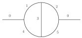
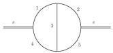
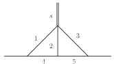
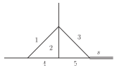
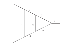
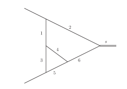
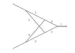
Figure 1: The bosonic electroweak two-loop topologies of the $Z{\bar{b}}b$ vertex.

2.1 The electroweak one-loop corrections to the $Z$-boson vertex

Around 1980 it became evident that the Glashow/Salam/Weinberg model might become the electroweak Standard Model. Consequently, some more elaborated loop calculations became meaningful.

Seen from today, the one-loop calculations of that time look quite simple. One had to understand complex logarithms, the Euler dilogarithm $\mathrm{Li}_{2}$, and to read basically two seminal papers by ’t Hooft and Veltman [35] and by Passarino and Veltman [36]. Among the first substantial, independent electroweak projects was a study in the unitary gauge by the Dubna group, founded by Dima Bardin. They studied complete electroweak radiative corrections for decays and scattering processes, including $e^{+}e^{-}\to{\bar{f}}f$ and $Z\to{\bar{f}}f$, assuming all fermions being massless. In [37], no expanded numerics was performed. Triggered partly by the detection of $Z\to l^{+}l^{-}$ by the UA1 and UA2 experiments at CERN, there were several calculations of $Z$-decay into leptons [38, 39], also under the assumption of massless fermions. The decay $Z\to{\bar{b}}b$ gets contributions from $m_{t}$-dependent vertex contributions, and it is not covered by these calculations, if the top quark is heavy. The top quark mass was unknown at that time, but the experimental mass limits were growing up. People at Dubna (Akhundov, Bardin, Riemann) observed that one can cover the amplitude with account of the additional $m_{t}$-dependent terms by adding up two known pieces:
${\cal M}(Z\to{\bar{q}}q)$ with $m_{q}=0$, and
${\cal M}(Z\to{\bar{q}_{1}}q_{2})$ with $q_{1},q_{2}$ having the same isospin, but $q_{1}\neq q_{2}$.
The first piece was known from [37], and the second one, non-vanishing only if a loop fermion mass is non-vanishing, from a study of flavor-nondiagonal $Z$ decays [40]. So the two were combined and accomplished by an independent recalculation of the whole $Z{\bar{b}}b$ amplitude. The preprint JINR-E2-85-617 appeared in August 1985, and soon later the publication [41]. The language of $\rho_{Z}$ and $\kappa_{Z}$ for the radiative corrections was used there, and the Fortran program ZRATE became the first piece of the electroweak Standard Model library of the ZFITTER project [7, 16, 42]. To give an example of the notation of form factors, we reproduce from [5] the leading terms of the additional top quark corrections to the $Z{\bar{b}}b$ vertex compared to the $Z{\bar{d}}d$ vertex:

$$\rho_{b}^{Z}=\rho_{d}^{Z}-2\frac{\Delta_{b}(m_{t}^{2})}{a_{b}},$$ (75)

$$\kappa_{b}^{Z}=\kappa_{d}^{Z}+\frac{\Delta_{b}(m_{t}^{2})}{a_{b}}.$$ (76)

The exact form factors have been implemented in ZFITTER. In the limit of large t-quark mass, the leading terms are given by [41]:

$$\frac{\Delta_{b}(m_{t}^{2})}{a_{b}}=\frac{\alpha}{4\pi\sin^{2}\theta_{W}}|V_{tb}|^{2}\frac{1}{2}\left[\frac{m_{t}^{2}}{M_{W}^{2}}+\left(\frac{8}{3}+\frac{1}{6\cos^{2}\theta_{W}}\right)\log\frac{m_{t}^{2}}{M_{W}^{2}}\right],$$ (77)

where $V_{tb}$ is the $(t,b)$ Kobayashi-Maskawa mixing matrix element. The ZFITTER calculations use the normalization $a_{b}=1$. In the above, the matrix element

$${\cal M}_{b} \sim \sqrt{\frac{G_{\mu}}{\sqrt{2}}M_{Z}^{2}}\epsilon^{\beta}\sqrt{\rho_{b}^{Z}}a_{b}{\bar{u}}\left[\gamma_{\beta}(1+\gamma_{5})-4\sin^{2}\theta_{W}\kappa_{b}^{Z}\gamma_{\beta}\right]u.$$ (78)

has been used.

The form factors for the $e^{+}e^{-}\to{\bar{f}}f$ scattering matrix element are related to those for the $Z\to{\bar{f}}f$ decay matrix element,

$$\rho_{eb} = \rho_{ed}-\frac{\Delta_{b}(m_{t}^{2})}{a_{b}},$$ (79)

$$\kappa_{b} = \kappa_{d}+\frac{\Delta_{b}(m_{t}^{2})}{a_{b}},$$ (80)

$$\kappa_{eb} = \kappa_{ed}+\frac{\Delta_{b}(m_{t}^{2})}{a_{b}},$$ (81)

with $\kappa_{e}$ unchanged.

At the official ZFITTER webpage http://sanc.jinr.ru/users/zfitter/ one may find the many additional publications on which the ZFITTER software is founded.

When the opening of LEP 1 at CERN approached, with a potential to observe the decays $Z\to{\bar{b}}b$, several further one-loop calculations were published: in October 1987 [43], in January 1988 [44], in January 1988 [45], in July 1988 [46], in 1990 [47]. Just to mention, the one-loop terms of our present code for the $Z{\bar{b}}b$ vertex remained unpublished (A. Freitas).

2.2 Known higher order corrections to the $Z{\bar{b}}b$ vertex

There are several higher-order corrections to the $Z{\bar{b}}b$ vertex known: the ${\mathcal{O}}(\alpha\alpha_{\mathrm{s}})$ QCD corrections [48, 49, 50, 51, 52, 53, 54], partial corrections of order ${\mathcal{O}}(\alpha_{\mathrm{t}}\alpha_{\mathrm{s}}^{2})$ [55, 56], partial corrections of order ${\mathcal{O}}(\alpha^{2}\alpha_{\mathrm{t}})$ and ${\mathcal{O}}(\alpha_{\mathrm{t}}^{3})$ [57, 58], the Standard Model two-loop prediction of $M_{\mathrm{W}}$ from the Fermi constant $G_{\mu}$ [59], partial corrections of order ${\mathcal{O}}(\alpha_{\mathrm{t}}\alpha_{\mathrm{s}}^{3})$ [60, 61, 62], the fermionic electroweak two-loop corrections [34]. Further references to be mentioned here are [15, 63, 64, 65, 10, 66, 67].

3 The bosonic $Z{\bar{b}}b$ topologies

The bosonic electroweak two-loop corrections to the $Z{\bar{b}}b$ vertex were the last missing piece for the prediction of $\sin^{2}\theta_{\rm eff}^{\rm b}$. We could use the calculational scheme as it was worked out in [10, 34] and work quoted therein. We calculated the ${\cal O}(700)$ unknown bosonic Feynman diagrams with two methods, in order to have two independent numerical results. One method relied on sector decomposition, and we used the publicly available packages FIESTA 3 [68] and SecDec 3 [69]. Both of them can apply contour deformation and are applicable to Minkowskian kinematics, as it is met here. The second method uses Mellin-Barnes representations for the Feynman integrals. For this, one may use the MB suite, publicly available at the MBtools webpage [70], and software from the Katowice webpage [71]. We had to develop two new tools. For the treatment of non-planar Feynman integrals, we developed AMBRE 3 [72, 73, 74], to complete the AMBRE versions 1 and 2 for planar cases [75]. The package MBnumerics [76] delivers a stable 8-digit numerical treatment of Feynman integrals with presently up to four dimensionless scales in the Minkowskian region. It was also essential, that both methods can automatically treat ultraviolet and infrared singularities. While the sector decomposition method had problems with few infrared divergent one- or two-scale integrals, the MB-method tends to fail for integrals with a larger number of scales. Nevertheless, we derived two precise, independent results for all the integrals needed. Details of the complete calculation have been reported in [1, 77] and in the transparencies of this talk at LL2016 [78], so we may restrict ourselves here to some pedagogical remarks.

3.1 The non-planar one-scale integral $I_{15}(\textrm{0H0W0txZ})$

As an example we compare several calculations of a non-planar two-loop vertex integral with one massive line and only one scale, $s=M_{Z}^{2}$, $I_{15}$(0H0W0txZ). It is shown in figure 2 and depends on one parameter $s/M_{Z}^{2}=1+i\epsilon$. A first calculation goes back to 1998 [79], so we could use the result as a cross-check of our own calculation with the Mellin-Barnes method [77, 1]. This was an important check, because an attempt to calculate the integral with the sector decomposition method in Minkowskian space-time failed.

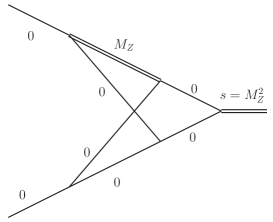
Figure 2: A non-planar vertex with one massive line.

The integral $I_{15}$(0H0W0txZ) is (up to some sign convention) the integral $N_{3}$ of [79]:

$$-N_{3} = I_{15}(\textrm{0H0W0txZ})$$

$$= \frac{e^{2\gamma_{E}\epsilon}}{\pi^{d}}\int\frac{d^{d}k_{1}d^{d}k_{2}}{D[k_{1},0]D[k_{1}-k_{2},0]D[k_{2},0]D[k_{2}+p_{2},0]D[k_{1}+k_{2}+p_{2},0]D[k_{1}-k_{2}+p_{1},M_{Z}]}.$$

The MB-representation is derived with calls to the packages PlanarityTest [72, 80] and AMBRE 3 [73, 74]. The $U$- and $F$-polynomials are: Upoly1 = x[1]x[2] + x[1]x[3] + x[2]x[3] + x[1]x[4] + x[3]x[4] + x[1]x[5] + x[2]x[5] + x[4]x[5] + x[2]x[6] + x[3]x[6] + x[4]x[6] + x[5]x[6] Fpoly2 = Upoly1 MZ^2 x[4] - s x[1]x[4]x[5] - s x[1]x[2]x[6] - s x[1]x[3]x[6] - s x[2]x[3]x[6] - s x[1]x[4]x[6] - s x[1]x[5]x[6] A naive MB-representation would become high-dimensional, and it would be plagued by the occurrence of terms containing the ill-defined expression $\Gamma[0]$. A dedicated introduction of Cheng-Wu variables leads to the following integrands for the $x$-integrations:

Upoly2 = v[1] + v[2] v[3]

Fpoly2 = + MZ^2 Upoly2 C[2]v[3] - s A[1]A[2]v[1]^2
         - s A[2]B[1]C[1]v[1]v[2]v[3] - s A[1]B[2]C[2]v[1]v[2]v[3]

The $x$-integrations over v[i] can be easily performed, and we remain, from the four additive terms in Fpoly2, with a three-dimensional MB-integral:

N3 ~  (-s)^(-2-2eps)  Gamma[-eps]
      (-(s/MZ^2))^-z2 Gamma[-eps-z1] Gamma[-z1] Gamma[-eps-z2] Gamma[-z2]
        Gamma[-1-2eps-z1-z3] Gamma[-1-2eps-z2-z3] Gamma[-1-2eps-z1-z2-z3]
        Gamma[-z3] Gamma[1+z3]^2 Gamma[1+z1+z3] Gamma[2+2eps+z1+z2+z3])
        / (Gamma[-2eps-z1] Gamma[-3eps-z2] Gamma[-2eps-z2] Gamma[-2eps-z1-z2])

When continuing in eps with the package MB.m [81], we derive for vanishing, but finite $\epsilon$ a two-dimensional and a three-dimensional MB-representation:

N3 ~
{
MBint[ ((-s)^(-2-2eps) Gamma[-2eps] Gamma[-eps]
(-(s/MZ^2))^-z2 Gamma[-eps-z2] Gamma[-z2]^2 Gamma[1+z2] Gamma[-1-2eps-z2-z3]
Gamma[-z3] Gamma[1+z3] Gamma[1+eps+z3] Gamma[1+2eps+z3])
 / (Gamma[-3eps-z2] Gamma[-2eps-z2] Gamma[1-z2+z3]),
{{eps->0},{z2->-0.42644,z3->-0.826119}} ],

MBint[ ((-s)^(-2-2eps) Gamma[-eps]
 (-(s/MZ^2))^-z2 Gamma[-eps-z1] Gamma[-z1] Gamma[-eps-z2] Gamma[-z2]
 Gamma[-1-2eps-z1-z3] Gamma[-1-2eps-z2-z3] Gamma[-1-2eps-z1-z2-z3]
 Gamma[-z3]  Gamma[1+z3]^2 Gamma[1+z1+z3]  Gamma[2+2eps+z1+z2+z3])
 / (Gamma[-2eps-z1] Gamma[-3eps-z2] Gamma[-2eps-z2] Gamma[-2 eps-z1-z2]),
{{eps->0},{z1->-0.268281,z2->-1.00065,z3->-0.171895}} ]
}

Applying MB [81] and MBnumerics [76], we get:

$$N_{3} = \frac{1}{\epsilon^{2}}(1.23370055013617-i~{}6.20475892887384\times 10^{-13})$$

$$+~{}\frac{1}{\epsilon}(2.8902545096591976+i~{}3.875784585038738)$$

$$+~{}({\color[rgb]{0,0,0}-0.778599608}3247692-i~{}{\color[rgb]{0,0,0}4.1235126}00516016).$$

The integral N3, according to equation (D.11) of [79], is with $z~{}=~{}s/M_{Z}^{2}~{}=~{}1+i\epsilon$:

$$N_{3} = \frac{1}{s^{2}}\sum_{n=1}^{\infty}{\color[rgb]{0,0,0}(-z)^{n}}\Biggl{\{}\frac{1}{\epsilon^{2}}\Biggl{[}-\frac{1}{2}\zeta_{2}+K_{2}(n-1)\Biggr{]}$$

$$+~{}\frac{1}{\epsilon}\Bigl{[}-\frac{1}{2}\zeta_{3}-2\zeta_{2}S_{1}(n-1)+2S_{3}(n-1)-2K_{3}(n-1)+4S_{1}(n-1)K_{2}(n-1)$$

$$+~{}(\zeta_{2}-S_{2}(n-1)){\color[rgb]{0,0,0}\ln(-z)}\Biggr{]}$$

$$+~{}\Biggl{[}-\zeta_{4}-2\zeta_{3}S_{1}(n-1)-7\zeta_{2}S_{2}(n-1)-4\zeta_{2}S_{1}(n-1)^{2}+7\zeta_{2}K_{2}(n-1)-\frac{7}{2}S_{4}(n-1)$$

$$+~{}\frac{7}{2}S_{2}(n-1)^{2}+6S_{1}(n-1)S_{3}(n-1)+2S_{13}(n-1)+8K_{4}(n-1)$$

$$-~{}8S_{1}(n-1)K_{3}(n-1)+8S_{1}(n-1)^{2}K_{2}(n-1)$$

$$+~{}\Bigl{(}\zeta_{3}+4\zeta_{2}S_{1}(n-1)-S_{12}(n-1)-3S_{1}(n-1)S_{2}(n-1)-4K_{3}(n-1)\Bigr{)}{\color[rgb]{0,0,0}\ln(-z)}$$

$$+~{}\Bigl{(}-\zeta_{2}+\frac{1}{2}S_{2}(n-1)+K_{2}(n-1)\Bigr{)}{\color[rgb]{0,0,0}\ln^{2}(-z)}\Biggr{]}\Biggr{\}}.$$

The expression contains harmonic sums [82, 83, 84]:

$$S_{a}(n) = \sum_{j=1}^{n}{1}/{j^{a}},$$ (85)

$$K_{a}(n) = -\sum_{j=1}^{n}(-1)^{j}/{j^{a}},$$ (86)

$$S_{ab}(n) = \sum_{j=1}^{n}{S_{b}(j-1)}/{j^{a}},$$ (87)

The sum $N_{3}$ converges both in the Euklidean and the Minkowskian kinematics, but very slowly, so that it would need many terms in order to get our accuracy goal of eight digits. The N3 evaluated with 200 terms gives e.g.:

time = 4.060519 sec       for 200 terms of the sum

N3 = (0.4 + 4 x I)

   + 1/eps x (2.8 + 3.87 x I) + 1 /eps^2 x (1.23 + 0 x I)

The agreement, with several thousand terms (few hours running time), is suffiently good in order to see that the results from the numerical MB-approach are reasonable. One may improve the comparison. In fact, in appendix E of [79], the necessary harmonic sums are explicitly performed. We derive:

$$\phi(z)=\frac{1}{2}S_{1,2}(z^{2})-S_{1,2}(z)-S_{1,2}(-z)+\ln(1-z)\text{Li}_{2}(-z)$$ (88)

and

$$-\frac{s^{2}z}{1+z}~{}{\color[rgb]{0,0,0}{N_{3}}} = ~{}~{}{\color[rgb]{0,0,0}{\frac{1}{\epsilon^{2}}}}\left[-\frac{\zeta_{2}}{2}-\text{Li}_{2}(z)\right]$$

$$+~{}{\color[rgb]{0,0,0}{\frac{1}{\epsilon}}}\biggl{[}-\frac{1}{2}\zeta_{3}-2\zeta_{2}\text{Li}_{2}(-z)+2\text{Li}_{3}(-z)+2\text{Li}_{3}(z)+4\bigl{[}\phi(-z)-S_{1,2}(z)-\text{Li}_{3}(-z)\bigr{]}$$

$$+~{}(\zeta_{2}-\text{Li}_{2}(-z))\ln(-z)\biggr{]}$$

$$-~{}\frac{s^{2}z}{1+z}~{}{\color[rgb]{0,0,0}{N_{3}^{\text{const}}}}$$

Further,

$$\frac{s^{2}(-z)}{1+z}~{}{\color[rgb]{0,0,0}{N_{3}^{\text{const}}}} = -\zeta_{4}+2\zeta_{3}\ln(1+z)-7\zeta_{2}\text{Li}_{2}(-z)-4~{}\zeta_{2}\left[-\ln(1-r)^{2}+\text{Li}_{2}(-z)\right]$$

$$+7~{}\zeta_{2}\text{Li}_{2}(z)-\frac{7}{2}\text{Li}_{4}(-z)+\frac{7}{2}\left[\text{Li}_{2}(-z)^{2}+\text{Li}_{4}(-z)-S_{2,2}(-z)\right]$$

$$+~{}6\bigl{[}(\text{Li}_{4}(-z)-\ln(1+z)\text{Li}_{3}(-z)-\frac{1}{2}\text{Li}_{2}(-z)^{2}+S_{2,2}(-z)\bigr{]}$$

$$+2~{}\left[-\ln(1+z)\text{Li}_{3}(-z)-\frac{1}{2}\text{Li}_{2}(-z)^{2}\right]+8\text{Li}_{4}(z)$$

$$-~{}8\left[-\text{Li}_{4}(z)-S_{2,2}(z)-\int_{0}^{-z}\frac{dt}{1-t}\text{Li}_{3}(-t)\right]$$

$$+8\biggl{[}-\text{Li}_{4}(z)-\frac{1}{2}S_{2,2}(z)-2S_{1,3}(z)+\phi(-z)[\ln(-z)-2\ln(1+z)]$$

$$-\int_{0}^{-z}\frac{dt}{1-t}[(2\ln(1-t)-\ln(t))\text{Li}_{2}(-t)+2\text{Li}_{3}(-t)+2S_{1,2}(-t)]\biggr{]}$$

$$+\Bigl{[}\zeta_{3}-4\zeta_{2}\ln(1+z)+\bigl{[}\ln(1+z)\text{Li}_{2}(-z)+S_{1,2}(-z)\bigr{]}$$

$$-~{}3\bigl{(}\text{Li}_{3}(-z)+(-\ln(1+z)\text{Li}_{2}(-z)-S_{1,2}(-z)\bigr{)}-4\text{Li}_{3}(z)\Bigr{]}\ln(-z)$$

$$+\Bigl{[}-\zeta_{2}+\frac{1}{2}\text{Li}_{2}(-z)+\text{Li}_{2}(z)\Biggr{]}\ln^{2}(-z)$$

The result is expressed in terms of polylogarithms, plus the few harmonic polylogarithms which are needed to close the basis of weight four. For a systematic numerical calculation of the expressions here in terms of harmonic polylogarithms $H[x,a,b,c,d],a,b,c,d=\pm 1,0$, see e.g. appendix B of [85], which is implemented in the Mathematica package HPL4num.m [86] and checked with the Mathematica package HPL [87]. The most compact representation of the integral at the $Z$ boson mass shell was obtained with the aid of Jacob Ablinger, Johannes Blümlein, Carsten Schneider and Arnd Behring (priv. commun.):

$$N_{3,-2}(z) = (z\zeta_{2})/(2(1+z))+(z\text{Li}_{2}(z))/(1+z),$$ (91)

$$N_{3,-2}(1+i~{}\epsilon) = \frac{3\zeta_{2}}{4},$$ (92)

$$N_{3,-1}(z) = \frac{z}{2(z+1)}\bigl{[}(-4H(-1,z)(2H(0,1,z)+\zeta_{2})+8H(0,-1,1,z)$$

$$-~{}4H(0,0,-1,-z)+4H(0,0,-1,z)+8H(0,1,-1,z)+8H(0,1,1,z)$$

$$-~{}2\ln(-z)H(0,-1,z)-2~{}\zeta_{2}\ln(-z)+\zeta_{3})\bigr{]},$$

$$N_{3,-1}(1+i~{}\epsilon) = -3\ln(2)\zeta_{2}+\frac{21}{4}\zeta_{3}+i~{}\frac{3}{4}\pi\zeta_{2}.$$ (94)

We confirm with $N_{3}(1+i~{}\epsilon)$ the 9 digits accuracy obtained with AMBRE/MB/MBnumerics given in (3.1):

$$N_{3,0}(1+i~{}\epsilon) = 24\text{Li}_{4}(1/2)+\ln^{4}(2)-\frac{351}{80}\zeta^{2}_{2}-I~{}3\ln(2)2\pi\zeta_{2}-i~{}\frac{63}{16}\pi\zeta_{3}$$

$$= 0.77859960898762168563452805690$$

$$-i~{}4.12351259333642272648103365383.$$

At the end of this section we like to mention, as an additional calculational alternative, a quite recent numerical approach to single-scale Feynman integrals [88].

4 Results

The electroweak bosonic two-loop contribution to the weak mixing angle is:

$$\Delta\kappa_{\mathrm{b}}^{(\alpha^{2},\rm bos)}=-0.9855\times 10^{-4}.$$ (96)

The value $-1.0276\times 10^{-4}$, presented as preliminary result at LL2016, was based on the input parameter list of [78] which differs slightly from the input list of table 1 of [1], which is applied here. This value amounts to about $\frac{1}{4}$ of the leptonic corrections to $\kappa_{b}$ and $\sin^{2}\theta_{\rm eff}^{\rm b}$. The corrections to the weak mixing angle are shown in table 2. The biggest corrections come from the one-loop electroweak contributions, followed by mixed electroweak-QCD corrections of order $\alpha\alpha_{s}$. All the other corrections, including the new bosonic electroweak two-loop corections, are of the same order, at the $10^{-4}$ level. For a per mille measurement, it is good to know them, but they will not influence the data analysis numerically.

Table 1: Reference values used in the numerical analysis, from Ref. [89].

Parameter	Value	Range
$M_{\mathrm{Z}}$	91.1876 GeV	$\pm 0.0042~{}\mbox{GeV}$
$\Gamma_{\mathrm{Z}}$	2.4952 GeV
$M_{\mathrm{W}}$	80.385 GeV	$\pm 0.030~{}\mbox{GeV}$
$\Gamma_{\mathrm{W}}$	2.085 GeV
$M_{\mathrm{H}}$	125.1 GeV	$\pm 5.0~{}\mbox{GeV}$
$m_{\mathrm{t}}$	173.2 GeV	$\pm 4.0~{}\mbox{GeV}$
$\alpha_{\mathrm{s}}$	0.1184	$\pm 0.0050$
$\Delta\alpha$	$0.0590$	$\pm 0.0005$

Table 2: Comparison of different orders of radiative corrections to $\Delta\kappa_{\mathrm{b}}$, using the input parameters in 1. Numerical values taken from [1].

Order	Value [$10^{-4}$]
$\alpha$	468.945
$\alpha\alpha_{\mathrm{s}}$	$-42.655$
$\alpha_{\mathrm{t}}\alpha_{\mathrm{s}}^{2}$	$-7.074$
$\alpha_{\mathrm{t}}\alpha_{\mathrm{s}}^{3}$	$-1.196$
$\alpha_{\mathrm{t}}^{2}\alpha_{\mathrm{s}}$	1.362
$\alpha_{\mathrm{t}}^{3}$	0.123
$\alpha^{2}_{\mathrm{ferm}}$	3.866
$\alpha^{2}_{\mathrm{bos}}$	$-0.986$

For the corresponding fitting formula for $\sin^{2}\theta_{\rm eff}^{\rm b}$, we refer to [1]. An analysis tool for the consistent 1 per mille treatment of realistic observables, pseudo-observables, and two-loop predictions to them, is not available for the $Z$ boson resonance, although ZFITTER is a very good approximation and suffices for the presently available accuracy of data.

References

- [1] I. Dubovyk, A. Freitas, J. Gluza, T. Riemann, J. Usovitsch, The two-loop electroweak bosonic corrections to , Phys. Lett. B762 (2016) 184–189. cmttcmttcmttcmttarXiv:1607.08375, cmttcmttcmttcmttdoi:10.1016/j.physletb.2016.09.012.
- [2] M. Baak et al., Gfitter 2.1 (Jan 2015), http://project-gfitter.web.cern.ch/project-gfitter/Software/index.html.
- [3] D. Bardin, C. Burdik, P. C. Khristova, T. Riemann, Electroweak radiative corrections to deep inelastic scattering at HERA. Neutral current scattering, Z. Phys. C42 (1989) 679. cmttcmttcmttcmttdoi:10.1007/BF01557676.
- [4] D. Y. Bardin, M. S. Bilenky, T. Riemann, M. Sachwitz, H. Vogt, P. C. Christova, DIZET: A program package for the calculation of electroweak one loop corrections for the process around the peak, Comput. Phys. Commun. 59 (1990) 303–312. cmttcmttcmttcmttdoi:10.1016/0010-4655(90)90179-5.
- [5] D. Bardin, M. Bilenky, A. Chizhov, O. Fedorenko, S. Ganguli, A. Gurtu, M. Lokajicek, G. Mitselmakher, A. Olshevsky, J. Ridky, S. Riemann, T. Riemann, M. Sachwitz, A. Sazonov, A. Schaile, Y. Sedykh, I. Sheer, L. Vertogradov, ZFITTER: An analytical program for fermion pair production in annihilation (1992). cmttcmttcmttcmttarXiv:hep-ph/9412201.
- [6] D. Bardin, P. Christova, M. Jack, L. Kalinovskaya, A. Olchevski, S. Riemann, T. Riemann, ZFITTER v.6.21: A semianalytical program for fermion pair production in annihilation, Comput. Phys. Commun. 133 (2001) 229–395. cmttcmttcmttcmttarXiv:hep-ph/9908433, cmttcmttcmttcmttdoi:10.1016/S0010-4655(00)00152-1.
- [7] A. Akhundov, A. Arbuzov, S. Riemann, T. Riemann, The ZFITTER project, Phys. Part. Nucl. 45 (2014) 529–549. cmttcmttcmttcmttarXiv:1302.1395, cmttcmttcmttcmttdoi:10.1134/S1063779614030022.
- [8] A. Leike, S. Riemann, T. Riemann, mixing in presence of standard weak loop corrections. cmttcmttcmttcmttarXiv:hep-ph/9808374.
- [9] D. Bardin, M. Bilenky, G. Mitselmakher, T. Riemann, M. Sachwitz, A realistic approach to the standard peak, Z. Phys. C44 (1989) 493. cmttcmttcmttcmttdoi:10.1007/BF01415565.
- [10] M. Awramik, M. Czakon, A. Freitas, Electroweak two-loop corrections to the effective weak mixing angle, JHEP 11 (2006) 048. cmttcmttcmttcmttarXiv:hep-ph/0608099, cmttcmttcmttcmttdoi:10.1088/1126-6708/2006/11/048.
- [11] R. Stuart, Gauge invariance, analyticity and physical observables at the resonance, Phys. Lett. B262 (1991) 113–119. cmttcmttcmttcmttdoi:10.1016/0370-2693(91)90653-8.
- [12] H. Veltman, Mass and width of unstable gauge bosons, Z. Phys. C62 (1994) 35–52. cmttcmttcmttcmttdoi:10.1007/BF01559523.
- [13] A. Leike, T. Riemann, J. Rose, S matrix approach to the Z line shape, Phys. Lett. B273 (1991) 513–518. cmttcmttcmttcmttarXiv:hep-ph/9508390, cmttcmttcmttcmttdoi:10.1016/0370-2693(91)90307-C.
- [14] T. Riemann, Cross-section asymmetries around the Z peak, Phys. Lett. B293 (1992) 451–456. cmttcmttcmttcmttarXiv:hep-ph/9506382, cmttcmttcmttcmttdoi:10.1016/0370-2693(92)90911-M.
- [15] D. Bardin, A. Leike, T. Riemann, M. Sachwitz, Energy dependent width effects in annihilation near the Z boson pole, Phys. Lett. B206 (1988) 539–542. cmttcmttcmttcmttdoi:10.1016/0370-2693(88)91625-5.
- [16] D. Bardin, M. Bilenky, P. Christova, M. Jack, L. Kalinovskaya, A. Olchevski, S. Riemann, T. Riemann, ZFITTER v.6.21: A semi-analytical program for fermion pair production in annihilation, Comput. Phys. Commun. 133 (2001) 229–395. cmttcmttcmttcmttarXiv:hep-ph/9908433, cmttcmttcmttcmttdoi:10.1016/S0010-4655(00)00152-1.
- [17] T. Riemann, S-matrix Approach to the Resonance, Acta Phys. Polon. B46 (2015) 2235. cmttcmttcmttcmttdoi:10.5506/APhysPolB.46.2235.
- [18] D. Bardin, M. Grünewald, G. Passarino, Precision calculation project report. cmttcmttcmttcmttarXiv:hep-ph/9902452.
- [19] ALEPH collab., DELPHI collab., L3 collab., OPAL collab., SLD collab., LEP Electroweak Working Group, SLD Electroweak Group, SLD Heavy Flavour Group, S. Schael, et al., Precision electroweak measurements on the resonance, Phys. Rept. 427 (2006) 257–454. cmttcmttcmttcmttarXiv:hep-ex/0509008, cmttcmttcmttcmttdoi:10.1016/j.physrep.2005.12.006.
- [20] D. Bardin, M. Bilenky, O. Fedorenko, T. Riemann, The electromagnetic contributions to annihilation into fermions in the electroweak theory. Total cross- section and integrated asymmetry (1988, Dubna preprint JINR-E2-88-324, unpublished, scan: http://www-lib.kek.jp/cgi-bin/img_index?8808103).
- [21] D. Y. Bardin, M. S. Bilenky, A. Chizhov, A. Sazonov, Y. Sedykh, T. Riemann, M. Sachwitz, The convolution integral for the forward - backward asymmetry in annihilation, Phys. Lett. B229 (1989) 405. cmttcmttcmttcmttdoi:10.1016/0370-2693(89)90428-0.
- [22] M. Bilenky, A. Sazonov, QED corrections at pole with realistic kinematical cuts, Dubna preprint JINR-E2-89-792, unpublished, scan: http://www-lib.kek.jp/cgi-bin/img_index?9003360 (1989).
- [23] D. Bardin, M. Bilenky, A. Chizhov, A. Sazonov, O. Fedorenko, T. Riemann, M. Sachwitz, Analytic approach to the complete set of QED corrections to fermion pair production in annihilation, Nucl. Phys. B351 (1991) 1–48. cmttcmttcmttcmttarXiv:hep-ph/9801208, cmttcmttcmttcmttdoi:10.1016/0550-3213(91)90080-H.
- [24] P. Christova, M. Jack, T. Riemann, Hard photon emission in with realistic cuts, Phys. Lett. B456 (1999) 264–269. cmttcmttcmttcmttarXiv:hep-ph/9902408, cmttcmttcmttcmttdoi:10.1016/S0370-2693(99)00528-6.
- [25] M. A. Jack, Semianalytical calculation of QED radiative corrections to with special emphasis on kinematical cuts to the final state. DESY-THESIS-2000-030. cmttcmttcmttcmttarXiv:hep-ph/0009068.
- [26] The TOPAZ0 homepage at Torino, http://personalpages.to.infn.it/~giampier/topaz0.html (June 2016).
- [27] G. Montagna, F. Piccinini, O. Nicrosini, G. Passarino, R. Pittau, TOPAZ0: A program for computing observables and for fitting cross-sections and forward-backward asymmetries around the peak, Comput. Phys. Commun. 76 (1993) 328–360. cmttcmttcmttcmttdoi:10.1016/0010-4655(93)90060-P.
- [28] G. Montagna, O. Nicrosini, G. Passarino, F. Piccinini, TOPAZO 2.0: A Program for computing deconvoluted and realistic observables around the peak, Comput. Phys. Commun. 93 (1996) 120–126. cmttcmttcmttcmttarXiv:hep-ph/9506329, cmttcmttcmttcmttdoi:10.1016/0010-4655(95)00127-1.
- [29] G. Montagna, O. Nicrosini, F. Piccinini, G. Passarino, TOPAZ0 4.0: A new version of a computer program for evaluation of deconvoluted and realistic observables at LEP-1 and LEP-2, Comput. Phys. Commun. 117 (1999) 278–289. cmttcmttcmttcmttarXiv:hep-ph/9804211, cmttcmttcmttcmttdoi:10.1016/S0010-4655(98)00080-0.
- [30] L3 collab., O. Adriani, et al., An S matrix analysis of the Z resonance, Phys. Lett. B315 (1993) 494–502. cmttcmttcmttcmttdoi:10.1016/0370-2693(93)91646-5.
- [31] S. Riemann, Search for a Z’ boson at the Z resonance with the L3 detector at the LEP accelerator, PhD thesis (RWTH Aachen, 1994), http://cds.cern.ch/record/270477/files/thesis-1994-riemann.pdf.
- [32] S. Kirsch, T. Riemann, SMATASY: A program for the model independent description of the Z resonance, Comput. Phys. Commun. 88 (1995) 89–108. cmttcmttcmttcmttarXiv:hep-ph/9408365, cmttcmttcmttcmttdoi:10.1016/0010-4655(95)00016-9.
-
[33]
M. Grünewald, S. Kirsch, T. Riemann, Fortran package SMATASY 6.42 (2 June
2005),
http://www.cern.ch/Martin.Grunewald/afs/public/smatasy/smata6_42.fortran. - [34] M. Awramik, M. Czakon, A. Freitas, B. Kniehl, Two-loop electroweak fermionic corrections to , Nucl. Phys. B813 (2009) 174–187. cmttcmttcmttcmttarXiv:0811.1364, cmttcmttcmttcmttdoi:10.1016/j.nuclphysb.2008.12.031.
- [35] G. ’t Hooft, M. Veltman, Scalar One Loop Integrals, Nucl. Phys. B153 (1979) 365–401. cmttcmttcmttcmttdoi:10.1016/0550-3213(79)90605-9.
- [36] G. Passarino, M. Veltman, One loop corrections for annihilation into in the Weinberg model, Nucl. Phys. B160 (1979) 151. cmttcmttcmttcmttdoi:10.1016/0550-3213(79)90234-7.
- [37] D. Y. Bardin, P. K. Khristova, O. Fedorenko, On the Lowest Order Electroweak Corrections to Spin 1/2 Fermion Scattering. 2. The One Loop Amplitudes, Nucl. Phys. B197 (1982) 1. cmttcmttcmttcmttdoi:10.1016/0550-3213(82)90152-3.
- [38] M. Consoli, S. Lo Presti, L. Maiani, Higher Order Effects and the Vector Boson Physical Parameters, Nucl. Phys. B223 (1983) 474–500. cmttcmttcmttcmttdoi:10.1016/0550-3213(83)90066-4.
- [39] J. Fleischer, F. Jegerlehner, Radiative and Decays: Precise Predictions from the Standard Model, Z. Phys. C26 (1985) 629. cmttcmttcmttcmttdoi:10.1007/BF01551808.
- [40] G. Mann, T. Riemann, Effective flavor changing weak neutral current in the standard theory and Z boson decay, Annalen Phys. 40 (1984) 334. cmttcmttcmttcmttdoi:10.1002/andp.19834950604.
- [41] A. Akhundov, D. Bardin, T. Riemann, Electroweak one loop corrections to the decay of the neutral vector boson, Nucl. Phys. B276 (1986) 1. cmttcmttcmttcmttdoi:10.1016/0550-3213(86)90014-3.
- [42] A. Arbuzov, M. Awramik, M. Czakon, A. Freitas, M. Grünewald, K. Mönig, S. Riemann, T. Riemann, ZFITTER: A semi-analytical program for fermion pair production in annihilation, from version 6.21 to version 6.42, Comput. Phys. Commun. 174 (2006) 728–758. cmttcmttcmttcmttarXiv:hep-ph/0507146, cmttcmttcmttcmttdoi:10.1016/j.cpc.2005.12.009.
- [43] J. Bernabeu, A. Pich, A. Santamaria, : A signature of hard mass terms for a heavy top, Phys. Lett. B200 (1988) 569. cmttcmttcmttcmttdoi:10.1016/0370-2693(88)90173-6.
- [44] W. Beenakker, W. Hollik, The width of the boson, Z. Phys. C40 (1988) 141. cmttcmttcmttcmttdoi:10.1007/BF01559728.
- [45] F. Jegerlehner, Precision tests of electroweak interaction parameters. In: R. Manka, M. Zralek (eds.), Proc. 11th Int. School of Theoretical Physics, Testing the Standard Model, Szczyrk, Poland, Sep 18-22, 1987 (Singapore, World Scientific, 1988), pp. 33-108. http://ccdb5fs.kek.jp/cgi-bin/img/allpdf?198801263.
- [46] F. Diakonos, W. Wetzel, The Z boson width to 1-loop. Preprint HD-THEP-88-21 (1988). http://ccdb5fs.kek.jp/cgi-bin/img/allpdf?198810239.
- [47] B. W. Lynn, R. G. Stuart, Electroweak radiative corrections to b quark production, Phys. Lett. B252 (1990) 676–682. cmttcmttcmttcmttdoi:10.1016/0370-2693(90)90505-Z.
- [48] A. Djouadi, C. Verzegnassi, Virtual very heavy top effects in LEP/SLC precision measurements, Phys. Lett. B195 (1987) 265–271. cmttcmttcmttcmttdoi:10.1016/0370-2693(87)91206-8.
- [49] A. Djouadi, vacuum polarization functions of the standard model gauge bosons, Nuovo Cim. A100 (1988) 357. cmttcmttcmttcmttdoi:10.1007/BF02812964.
- [50] B. A. Kniehl, Two loop corrections to the vacuum polarizations in perturbative QCD, Nucl. Phys. B347 (1990) 86–104. cmttcmttcmttcmttdoi:10.1016/0550-3213(90)90552-O.
- [51] B. A. Kniehl, A. Sirlin, Dispersion relations for vacuum polarization functions in electroweak physics, Nucl. Phys. B371 (1992) 141–148. cmttcmttcmttcmttdoi:10.1016/0550-3213(92)90232-Z.
- [52] A. Djouadi, P. Gambino, Electroweak gauge bosons selfenergies: Complete QCD corrections, Phys. Rev. D49 (1994) 3499–3511, Erratum: Phys. Rev. D53 (1996) 4111. cmttcmttcmttcmttarXiv:hep-ph/9309298, cmttcmttcmttcmttdoi:10.1103/PhysRevD.49.3499,10.1103/PhysRevD.53.4111.
- [53] A. Czarnecki, J. H. Kühn, Nonfactorizable QCD and electroweak corrections to the hadronic Z boson decay rate, Phys. Rev. Lett. 77 (1996) 3955–3958. cmttcmttcmttcmttarXiv:hep-ph/9608366, cmttcmttcmttcmttdoi:10.1103/PhysRevLett.77.3955.
- [54] R. Harlander, T. Seidensticker, M. Steinhauser, Complete corrections of order to the decay of the Z boson into bottom quarks, Phys. Lett. B426 (1998) 125–132. cmttcmttcmttcmttarXiv:hep-ph/9712228, cmttcmttcmttcmttdoi:10.1016/S0370-2693(98)00220-2.
- [55] L. Avdeev, J. Fleischer, S. Mikhailov, O. Tarasov, correction to the electroweak parameter, Phys. Lett. B336 (1994) 560–566, Erratum: Phys. Lett. B349 (1995) 597. cmttcmttcmttcmttarXiv:hep-ph/9406363, cmttcmttcmttcmttdoi:10.1016/0370-2693(94)90573-8.
- [56] K. Chetyrkin, J. H. Kühn, M. Steinhauser, Corrections of order to the parameter, Phys. Lett. B351 (1995) 331–338. cmttcmttcmttcmttarXiv:hep-ph/9502291, cmttcmttcmttcmttdoi:10.1016/0370-2693(95)00380-4.
- [57] J. J. van der Bij, K. G. Chetyrkin, M. Faisst, G. Jikia, T. Seidensticker, Three loop leading top mass contributions to the parameter, Phys. Lett. B498 (2001) 156–162. cmttcmttcmttcmttarXiv:hep-ph/0011373, cmttcmttcmttcmttdoi:10.1016/S0370-2693(01)00002-8.
- [58] M. Faisst, J. H. Kühn, T. Seidensticker, O. Veretin, Three loop top quark contributions to the parameter, Nucl. Phys. B665 (2003) 649–662. cmttcmttcmttcmttarXiv:hep-ph/0302275, cmttcmttcmttcmttdoi:10.1016/S0550-3213(03)00450-4.
- [59] M. Awramik, M. Czakon, A. Freitas, G. Weiglein, Precise prediction for the W boson mass in the standard model, Phys. Rev. D69 (2004) 053006. cmttcmttcmttcmttarXiv:hep-ph/0311148, cmttcmttcmttcmttdoi:10.1103/PhysRevD.69.053006.
- [60] Y. Schröder, M. Steinhauser, Four-loop singlet contribution to the parameter, Phys. Lett. B622 (2005) 124–130. cmttcmttcmttcmttarXiv:hep-ph/0504055, cmttcmttcmttcmttdoi:10.1016/j.physletb.2005.06.085.
- [61] K. G. Chetyrkin, M. Faisst, J. H. Kühn, P. Maierhofer, C. Sturm, Four-loop QCD corrections to the parameter, Phys. Rev. Lett. 97 (2006) 102003. cmttcmttcmttcmttarXiv:hep-ph/0605201, cmttcmttcmttcmttdoi:10.1103/PhysRevLett.97.102003.
- [62] R. Boughezal, M. Czakon, Single scale tadpoles and corrections to the parameter, Nucl. Phys. B755 (2006) 221–238. cmttcmttcmttcmttarXiv:hep-ph/0606232, cmttcmttcmttcmttdoi:10.1016/j.nuclphysb.2006.08.007.
- [63] M. Awramik, M. Czakon, Complete two loop bosonic contributions to the muon lifetime in the standard model, Phys. Rev. Lett. 89 (2002) 241801. cmttcmttcmttcmttarXiv:hep-ph/0208113, cmttcmttcmttcmttdoi:10.1103/PhysRevLett.89.241801.
- [64] A. Onishchenko, O. Veretin, Two loop bosonic electroweak corrections to the muon lifetime and interdependence, Phys. Lett. B551 (2003) 111–114. cmttcmttcmttcmttarXiv:hep-ph/0209010, cmttcmttcmttcmttdoi:10.1016/S0370-2693(02)03004-6.
- [65] A. Freitas, W. Hollik, W. Walter, G. Weiglein, Electroweak two loop corrections to the mass correlation in the standard model, Nucl. Phys. B632 (2002) 189–218, [Erratum: Nucl. Phys.B666,305(2003)]. cmttcmttcmttcmttarXiv:hep-ph/0202131, cmttcmttcmttcmttdoi:10.1016/S0550-3213(02)00243-2.
- [66] A. Freitas, Two-loop fermionic electroweak corrections to the Z-boson width and production rate, Phys. Lett. B730 (2014) 50–52. cmttcmttcmttcmttarXiv:1310.2256, cmttcmttcmttcmttdoi:10.1016/j.physletb.2014.01.017.
- [67] A. Freitas, Higher-order electroweak corrections to the partial widths and branching ratios of the Z boson, JHEP 1404 (2014) 070. cmttcmttcmttcmttarXiv:1401.2447, cmttcmttcmttcmttdoi:10.1007/JHEP04(2014)070.
- [68] A. V. Smirnov, FIESTA 3: cluster-parallelizable multiloop numerical calculations in physical regions, Comput. Phys. Commun. 185 (2014) 2090–2100. cmttcmttcmttcmttarXiv:1312.3186, cmttcmttcmttcmttdoi:10.1016/j.cpc.2014.03.015.
- [69] S. Borowka, G. Heinrich, S. P. Jones, M. Kerner, J. Schlenk, T. Zirke, SecDec 3.0: numerical evaluation of multi-scale integrals beyond one loop, Comput. Phys. Commun. 196 (2015) 470–491. cmttcmttcmttcmttarXiv:1502.06595, cmttcmttcmttcmttdoi:10.1016/j.cpc.2015.05.022.
- [70] M. Czakon (MB, MBasymptotics), D. Kosower (barnesroutines), A. Smirnov, V. Smirnov (MBresolve), K. Bielas, I. Dubovyk, J. Gluza, K. Kajda, T. Riemann (AMBRE, PlanarityTest), MBtools webpage, https://mbtools.hepforge.org/.
- [71] Silesian University at Katowice, webpage http://prac.us.edu.pl/$\sim$gluza/ambre.
- [72] K. Bielas, I. Dubovyk, PlanarityTest 1.1 (January 2014), a Mathematica package for testing the planarity of Feynman diagrams, http://us.edu.pl/~gluza/ambre/planarity/, [80].
- [73] I. Dubovyk, J. Gluza, T. Riemann, Non-planar Feynman diagrams and Mellin-Barnes representations with , J. Phys. Conf. Ser. 608 (2015) 012070. DESY 14–174 (13 April 2016). cmttcmttcmttcmttdoi:10.1088/1742-6596/608/1/012070.
- [74] I. Dubovyk, AMBRE 3.0 (1 Sep 2015), a Mathematica package representing Feynman integrals by Mellin-Barnes integrals, available at http://prac.us.edu.pl/~gluza/ambre/, [90, 73].
- [75] J. Gluza, K. Kajda, T. Riemann, AMBRE - a Mathematica package for the construction of Mellin-Barnes representations for Feynman integrals, Comput. Phys. Commun. 177 (2007) 879–893. cmttcmttcmttcmttarXiv:0704.2423, cmttcmttcmttcmttdoi:10.1016/j.cpc.2007.07.001.
- [76] I. Dubovyk, T. Riemann, J. Usovitsch, Numerical calculation of multiple MB-integral representations for Feynman integrals. J. Usovitsch, MBnumerics, a program in preparation, to be made available at http://prac.us.edu.pl/~gluza/ambre/.
- [77] I. Dubovyk, J. Gluza, T. Riemann, J. Usovitsch, Numerical integration of massive two-loop Mellin-Barnes integrals in Minkowskian regions, in: 13th DESY Workshop on Elementary Particle Physics: Loops and Legs in Quantum Field Theory (LL2016) Leipzig, Germany, April 24-29, 2016, 2016. cmttcmttcmttcmttarXiv:1607.07538.
- [78] I. Dubovyk, A. Freitas, J. Gluza, T. Riemann, J. Usovitsch, 30 years, 715 integrals, and 1 dessert, or: Bosonic contributions to the 2-loop Zbb vertex, talk at LL2016, 24-28 April 2016, Leipzig, Germany, to appear in the proceedings. https://indico.desy.de/getFile.py/access?contribId=63&sessionId=12&resId=0&materialId=slides&confId=12010.
- [79] J. Fleischer, A. Kotikov, O. Veretin, Analytic two loop results for selfenergy type and vertex type diagrams with one nonzero mass, Nucl. Phys. B547 (1999) 343–374. cmttcmttcmttcmttarXiv:hep-ph/9808242, cmttcmttcmttcmttdoi:10.1016/S0550-3213(99)00078-4.
- [80] K. Bielas, I. Dubovyk, J. Gluza, T. Riemann, Some Remarks on Non-planar Feynman Diagrams, Acta Phys. Polon. B44 (2013) 2249–2255. cmttcmttcmttcmttarXiv:1312.5603, cmttcmttcmttcmttdoi:10.5506/APhysPolB.44.2249.
- [81] M. Czakon, Automatized analytic continuation of Mellin-Barnes integrals, Comput. Phys. Commun. 175 (2006) 559–571. cmttcmttcmttcmttarXiv:hep-ph/0511200, cmttcmttcmttcmttdoi:10.1016/j.cpc.2006.07.002.
- [82] D. I. Kazakov, A. V. Kotikov, The Method of Uniqueness: Multiloop Calculations in QCD, Theor. Math. Phys. 73 (1988) 1264, [Teor. Mat. Fiz.73,348(1987)]. cmttcmttcmttcmttdoi:10.1007/BF01041909.
- [83] A. V. Kotikov, The Calculation of Moments of Structure Function of Deep Inelastic Scattering in QCD, Theor. Math. Phys. 78 (1989) 134–143, [Teor. Mat. Fiz.78,187(1989)]. cmttcmttcmttcmttdoi:10.1007/BF01018678.
- [84] D. I. Kazakov, A. V. Kotikov, On the value of the alpha-s correction to the Callan-Gross relation, Phys. Lett. B291 (1992) 171–176. cmttcmttcmttcmttdoi:10.1016/0370-2693(92)90139-U.
- [85] M. Czakon, J. Gluza, T. Riemann, Master integrals for massive two-loop bhabha scattering in QED, Phys. Rev. D71 (2005) 073009. cmttcmttcmttcmttarXiv:hep-ph/0412164, cmttcmttcmttcmttdoi:10.1103/PhysRevD.71.073009.
- [86] T. Riemann, HPL4num (05 Oct 2004), a Mathematica package for the numerical calculation of harmonic polylogarithms, available at http://prac.us.edu.pl/~gluza/ambre/, [85].
- [87] D. Maitre, HPL, a Mathematica implementation of the harmonic polylogarithms, Comput. Phys. Commun. 174 (2006) 222–240. cmttcmttcmttcmttarXiv:hep-ph/0507152, cmttcmttcmttcmttdoi:10.1016/j.cpc.2005.10.008.
- [88] J. Gluza, T. Jelinski, D. A. Kosower, Efficient evaluation of massive Mellin–Barnes integrals. cmttcmttcmttcmttarXiv:1609.09111.
- [89] K. Olive, et al., Review of Particle Physics, Chin. Phys. C38 (2014) 090001. cmttcmttcmttcmttdoi:10.1088/1674-1137/38/9/090001.
- [90] J. Gluza, K. Kajda, T. Riemann, V. Yundin, Numerical Evaluation of Tensor Feynman Integrals in Euclidean Kinematics, Eur. Phys. J. C71 (2011) 1516. cmttcmttcmttcmttarXiv:1010.1667, cmttcmttcmttcmttdoi:10.1140/epjc/s10052-010-1516-y.