The effect of delay on contact tracing

Abstract

We consider a model for an infectious disease in the onset of an outbreak. We introduce contact tracing incorporating a tracing delay. The effect of randomness in the delay and the effect of the length of this delay in comparison to the infectious period of the disease respectively to a latency period on the effect of tracing, given e.g. by the change of the reproduction number, is analyzed. We focus particularly on the effect of randomness in the tracing delay.

Keywords: Stochastic epidemic; contact tracing; branching process; reproduction number

1 Introduction

Contact tracing resp. partner notification programs are believed to be of central importance for the control of many infectious diseases: infected persons are questioned for recent potentially infectious contacts. In this way, further infected and infectious persons are identified in a targeted way, often quite early after infection. These persons can be treated and isolated, and the number of further infections can be reduced. For some emerging infections, data analysis indicates that contact tracing has proven to be a valuable measure – e.g. in the case of SARS [14] or Ebola [18]. For other infections, such as tuberculosis, contacts may be this casual that they are hardly recognized; in these cases it is under debate if contact tracing pays [20, 4, 7]. Still, our understanding of the effectiveness of contact tracing is incomplete. In particular, the consequences of the different time scales involved – latent period, typical time between contacts, and the delay in the tracing process – remain unclear.

As contact tracing depends on the detailed contact structure, it is – in contrast to e.g. mass screening – not immediately clear how to model this method appropriately. Local interactions and correlations have to be taken into account. In recent years, basically two different modelling approaches have been successfully developed. The first approach [5, 11, 10] relies on a fixed contact graph. The infection (as well as contact tracing) spreads via the edges of this graph, and is modeled as a stochastic contact process. Pair approximation yields a model consisting of ordinary differential equations (ODEs) that gasps the most important features of the dynamics. The mean value of the stochastic process is more or less met by these ODEs. This modeling approach gives in particular good results if the degree of nodes is large.

The second approach is based on a branching process, and in particular used to describe the onset of an outbreak [16, 17, 15]. On the tree of infecteds (the nodes are infected individuals, a directed edge points from infector to infectee) the tracing process takes place. If an individual is discovered, adjacent edges have (independently) a certain probability – the tracing probability – to be detected. As the underlying graph is directed, it is suggestive to define forward tracing (if the infector is discovered, infectees are traced) and backward tracing (if an infectee is discovered, the infector is traced). Even in the very early papers [9] this concept has been developed, and it has been discussed if forward- or backward tracing is more important.

In addition to these two mathematical approaches, a lot of work has been done based on simulation models [12, 13] and/or to understand the effect of contact tracing for certain diseases like influenza, SARS, tuberculosis or Ebola [6, 14, 7, 4, 18].

In the present work, we take up the discussion how a tracing delay – the time elapsing between the discovery of an infected individual and the identification of his/her infector and infectees – influences the efficiency of contact tracing. Fraser [8] and Kiss [12] already discussed the importance of a latent period for contact tracing: a latent period allows one to detect cases before they start to spread the diseases and in this makes contact tracing more effective. A tracing delay has the converse effect; persons may spread the infection also during the time that elapses between detection of an index case and their own detection by contact tracing. Only few models address this delay explicitly. Klinkenberg et al. [14] extends the work of Fraser et al. [8] by a tracing delay. Approximations of the next generation operator for contact tracing were developed. Another approach was used by Shaban et al. [19]. In that paper, a fixed contact network is considered (as in most pair approximation models), but the authors focus on the onset of an outbreak and use a branching process approximation of the process. They only take into account forward tracing. In principle, their model allows for general distributions for latency period and tracing delay, but the authors concentrate on the special case of exponential distributions. Ball et al. [2, 3] take up this idea. They also consider only forward tracing but assume a homogeneously mixing population. The authors formulate a multitype-branching process for detected individuals. This approach is mathematically particularly appealing, as the theory of branching processes can be used to derive analytical results.

In the present work we extend the methods developed in [16] to analyse delayed contact tracing with forward- and backward tracing. We do this analysis first for an epidemic with constant contact- and recovery rates, but extend the ideas also to non-constant rates, opening the possibility to also consider an infection with latent period. The central technique relies on the derivation of the probability that an individual is still infectious at a given age of infection. However, in general it is only possible to solve these equations numerically. Approximate solutions are derived for small tracing probabilities; also an approximation for the reproduction number is given. The influence of the timing (latent period and tracing delay) is discussed. We are particularly interested in the question how randomness in the tracing delay affects the efficiency of contact tracing as given by the reduction of the reproduction number, if forward- or backward tracing is more important, and how the interplay between the time scales involved (tracing delay, mean infectious period, and latency period) influences contact tracing.

2 Model and Analysis

We consider a randomly mixing, homogeneous population. Note that models assuming a homogeneous population may behave differently compared with models that assume an underlying contact graph, in particular of the contact graph is sparse. It depends on the disease which approach is more appropriate. In order to model contact tracing, we start off with an SIS/SIR- type of model, and focus on the onset of an epidemic (therefore we do not need to specify if a recovered person will be susceptible again or immune). In the long run, SIR and SIS models will, of course, behave differently. The contact rate is denoted by $\beta$. Infected persons recover at rate $\gamma$. With probability $p_{\text{obs}}$ recovered persons become index cases and trigger (at recovery) a tracing event. Tracing, however, does not take place immediately but with a random delay $T$, distributed with density $\phi$. We allow generalized functions for this density, such that a fixed delay is covered by the model. For each contact, the delay is an independent realization; it is not the case that the tracing delay e.g. only depends on the index case. Infector and infectees of the index case have, if they are still infectious at the time at which contact tracing actually takes place, a probability $p$ to be diagnosed. We consider two different modes: either a traced individual is again an index case (recursive tracing), or the contact tracing stops (one-step-tracing).

For technical reasons, we introduce the rates $\alpha=(1-p_{\text{obs}})\gamma$ and $\sigma=p_{\text{obs}}\gamma$, and consider $\alpha$ as the spontaneous recovery rate (no diagnosis), and $\sigma$ the recovery rate with direct (not via tracing) diagnosis of the infection. Note that we focus on the onset of the epidemic. Therefore, all contacts of an infected individual connect to susceptible individuals. The infection process without tracing is well approximated by a linear branching process (along the line of the argument of Ball and Donnelly [1], see also [16, 2]). Only tracing introduces dependencies between individuals. In order to analyze this process, we first look at backward tracing, then at forward tracing, and at the end we combine both processes to full tracing.

2.1 Backward tracing – recursive mode

Let us assume that only backward tracing takes place, and no forward tracing. We furthermore consider the recursive tracing mode. As usual, convolution of two functions $f$ and $g$ is defined by $(f\ast g)(a)=\int_{0}^{a}f(a-\tau)g(\tau)\,d\tau$. Furthermore, we define

$$f^{\#}(a)=\int_{0}^{a}f(\tau)\,d\tau=(1\ast f)(t).$$

Proposition 2.1

Let $\phi(t)$ denote the distribution of the tracing delay $T$, $\kappa_{-}(a)$ the probability to be infectious after time of infection $a$. Then,

$$\kappa_{-}^{\prime}(a)=-\kappa_{-}(a)\left\{\alpha+\sigma+p\,\beta\,\left[(\phi\ast(1-\kappa_{-}))(a)-\alpha(\phi\ast\kappa_{-}^{\#})(a)\right]\right\},\quad\kappa_{-}(0)=1.$$ (1)

Proof: We start off with the relation

$$\kappa_{-}^{\prime}(a)=-\kappa_{-}(a)\left\{\alpha+\sigma+\mbox{rate of tracing}\,(a)\right\}.$$

In order to obtain the rate of (direct or indirect) detection of an infected individual with age since infection $a$ , we subtract from the total removal rate (or hazard) $-\kappa_{-}^{\prime}(a)/\kappa_{-}(a)$ the rate of spontaneous removal $\alpha$,

$$\frac{-\kappa^{\prime}_{-}(a)}{\kappa_{-}(a)}-\alpha.$$

In order to compute the contribution of backward contact tracing to the removal rate, we consider the infectees (generated at rate $\beta$) that are still infectious after $c$ time units (probability $\kappa_{-}(c)$) and are detected at age of the infector $\tau$,

$$\int_{0}^{\tau}\beta\left(\frac{-\kappa^{\prime}_{-}(c)}{\kappa_{-}(c)}-\alpha\right)\kappa_{-}(c)\,dc.$$

These individuals increase the removal rate of the infector at age of infection $a$, if the tracing delay is precisely $a-\tau$ (probability density $\phi(a-\tau)$), and the infector is traced, indeed (probability $p$). That is,

$$\mbox{rate of tracing}\,(a)=p\,\int_{0}^{a}\phi(a-\tau)\int_{0}^{\tau}\beta\left(\frac{-\kappa^{\prime}_{-}(c)}{\kappa_{-}(c)}-\alpha\right)\kappa_{-}(c)\,dc\,d\tau$$

$$= p\,\beta\int_{0}^{a}\phi(a-\tau)\left((1-\kappa_{-}(\tau)-\alpha\kappa^{\#}_{-}(\tau)\right)\,d\tau=p\,\beta\,\left[(\phi\ast 1)(a)-(\phi\ast\kappa_{-})(a)-\alpha(\phi\ast\kappa_{-}^{\#})(a)\right].$$

We obtain the integro-differential equation stated above.

Let from now on $\widehat{\kappa}(a)=e^{-(\alpha+\sigma)a}$ for $a\geq 0$, and $\widehat{\kappa}(a)=0$ for $a<0$.

Proposition 2.2

The first order approximation of $\kappa_{-}(a)$ in $p$ reads

$$\kappa_{-}(a) = \widehat{\kappa}(a)-p\,p_{\text{obs}}\,\beta\,\widehat{\kappa}(a)\,\,(1\ast\phi\ast(1-\widehat{\kappa}))(a)+{\cal O}(p^{2}).$$ (2)

Proof: We go for a first order approximation. Note that $\kappa_{-}(a)$ does not only depend on $a$ but also on $p$ (and some other parameters that we keep constant). For a given $a$, we expand $\kappa_{-}(a)$ as a power series in $p$, viz.

$$\kappa_{-}(a)=\sum_{i=0}^{\infty}p^{i}\,\kappa_{-,i}(a).$$

In this formula, the functions $\kappa_{-,i}(a)$ do not depend on $p$ any more. We replace $\kappa_{-}(a)$ by this expansion in the integro-differential equation (1),

$$\sum_{i=0}^{\infty}p^{i}\,\kappa_{-,i}^{\prime}(a)=-\left(\sum_{i=0}^{\infty}p^{i}\,\kappa_{-,i}(a)\right)\left\{\alpha+\sigma+p\,\beta\,\left[(\phi\ast(1-\sum_{i=0}^{\infty}p^{i}\,\kappa_{-,i}))(a)-\alpha(\sum_{i=0}^{\infty}p^{i}\,\phi\ast\kappa_{-,i}^{\#})(a)\right]\right\},\quad\sum_{i=0}^{\infty}p^{i}\,\kappa_{-,i}(0)=1$$

and equate powers of $p$. We find for $p^{0}$ and $p^{1}$

$$\kappa_{-,0}^{\prime}(a) = -\kappa_{-,0}(a)(\alpha+\sigma),\qquad\kappa_{-,0}(0)=1,$$

$$\kappa_{-,1}^{\prime}(a) = -(\alpha+\sigma)\kappa_{-,1}(a)-\beta\,\kappa_{-,0}(a)\,\left[(\phi\ast 1)(a)-(\phi\ast\kappa_{-,0})(a)-\alpha(\phi\ast\kappa_{-,0}^{\#})(a)\right],\quad\kappa_{-,1}(0)=0.$$

Therefore, $\kappa_{-,0}(a)=e^{-(\alpha+\sigma)\,a}=\widehat{\kappa}(a)$ and, with $\kappa_{-,0}^{\#}(a)=(1-\widehat{\kappa}(a))/(\alpha+\sigma)$ we obtain that

$$\bigg{[}(\phi\ast 1)(a)-(\phi\ast\kappa_{-,0})(a)-\alpha(\phi\ast\kappa_{-,0}^{\#})(a)\bigg{]}=(\phi\ast(1-\widehat{\kappa}))(a)-\frac{\alpha}{\alpha+\sigma}(\phi\ast(1-\widehat{\kappa}))(a)$$

$$= \frac{\sigma}{\alpha+\sigma}(\phi\ast(1-\widehat{\kappa}))(a).$$

Hence, the first order correction of $\widehat{\kappa}$ by backward tracing reads

$$\kappa_{-,1}(a) = -\,\int_{0}^{a}e^{-(\alpha+\sigma)(a-\tau)}\,\frac{\beta\sigma}{\alpha+\sigma}e^{-(\alpha+\sigma)\tau}\,(\phi\ast(1-\widehat{\kappa}))(\tau)\,d\tau$$

$$= -\,\frac{\beta\sigma}{\alpha+\sigma}\widehat{\kappa}(a)\,\,(1\ast\phi\ast(1-\widehat{\kappa}))(a).$$

Therewith the result follows.

2.1.1 Special case: fixed delay

Assume that the tracing delay is a deterministic, fixed time period $T$. That is, $\phi(a)=\delta_{T}(a)$. Then,

$$(\phi\ast(1-\widehat{\kappa}))(a)=(1-\widehat{\kappa}(a-T))$$

for $a>T$ and zero else. Hence, for $a>T$,

$$(1\ast\phi\ast(1-\widehat{\kappa}))(a) = \int_{0}^{a}\phi\ast(1-\widehat{\kappa})(\tau)\,d\tau=\int_{T}^{a}(1-\widehat{\kappa}(a-T))\,d\tau$$

$$= (a-T)-\frac{1}{\alpha+\sigma}\,\left(1-e^{-(\alpha+\sigma)(a-T)}\right).$$

All in all, we obtain for $a<T$ that

$$\kappa_{-}(a)=e^{-(\alpha+\sigma)a}=\widehat{\kappa}(a)$$

and for $a>T$

$$\kappa_{-}(a)=\widehat{\kappa}(a)-p\,p_{\text{obs}}\,\beta\,\,\widehat{\kappa}(a)\,\,\left\{(a-T)-\frac{1-\widehat{\kappa}(a-T)}{\alpha+\sigma}\,\right\}+{\cal O}(p^{2}).$$

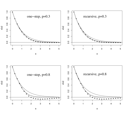
Figure 1: $\kappa_{-}(a)$ for backward tracing (one step, recursive tracing, $p=0.3$, and $p=0.8$, as indicated). Solid line: $\widehat{\kappa}(a)$, gray line: simulated data, dashed line: $\kappa_{-}(a)$ according to the theory, dots: first order approximation of $\kappa_{-}(a)$. Parameters: $\beta=2$, $\alpha=0.1$, $\sigma=0.9$, fixed tracing delay, $T=0.5$.

The numerical analysis shows an excellent agreement of theory as given by eq. (1) and simulation (figure 1). However, the first order approximation (2) is not valid any more if $p$ becomes large.

2.1.2 Special case: exponential delay

Apart of a fixed delay, an exponentially distributed delay is another natural choice. Let the mean value be $T$, $\phi(a)=e^{-a/T}/T$. We assume that $T(\alpha+\sigma)\not=1$. Straight forward computations yield

$$\kappa_{-}(a)=\widehat{\kappa}(a)-p\,p_{\text{obs}}\,\beta\,\widehat{\kappa}(a)\,\left\{a+T\,\,\,\frac{T(\alpha+\sigma)}{1-T(\sigma+\alpha)}\left((1-e^{-a/T})-\frac{1-\widehat{\kappa}(a)}{(T(\sigma+\alpha))^{2}}\right)\right\}+\mathcal{O}(p^{2}).$$

Figure 3 indicates that the exponentially distributed delay has a larger effect than the fixed delay. We come later back to this observation and discuss the presumable mechanism behind this finding.

2.1.3 Rates depending on age since infection

We generalize the model assumptions and allow for the case that $\beta$, $\alpha$ and $\sigma$ depend on the age since infection, e.g., $\beta=\beta(a)$. These relaxed assumptions allow to consider the interplay between contact tracing and a latency period. We only look at the fully recursive case, since the one-step tracing case is more simple.
The argument here parallels that of proposition 2.1. The rate at which an infectee is detected at age of infector $\tau$ is now given by

$$\int_{0}^{\tau}\beta(\tau-c)\left(\frac{-\kappa^{\prime}_{-}(c)}{\kappa_{-}(c)}-\alpha(c)\right)\kappa_{-}(c)\,dc.$$

Hence, the removal rate due to contact tracing reads

$$\mbox{rate of removal by contact tracing}(a)$$

$$= p\,\int_{0}^{a}\phi(a-\tau)\int_{0}^{\tau}\beta(\tau-c)\left(\frac{-\kappa^{\prime}_{-}(c)}{\kappa_{-}(c)}-\alpha(c)\right)\kappa_{-}(c)\,dc\,d\tau$$

$$= -p\,\int_{0}^{a}\phi(a-\tau)\int_{0}^{\tau}\bigg{(}\beta(\tau-c)\kappa^{\prime}_{-}(c)+\beta(\tau-c)\alpha(c)\kappa_{-}(c)\bigg{)}\,dc\,d\tau.$$

Unfortunately, in general this expression cannot be simplified. We obtain the integro-differential equation for $\kappa_{-}(a)$

$$\kappa_{-}^{\prime}(a)=-\kappa_{-}(a)\left(\sigma(a)+\alpha(a)-p\,\int_{0}^{a}\phi(a-\tau)\int_{0}^{\tau}\bigg{(}\beta(\tau-c)\kappa^{\prime}_{-}(c)+\beta(\tau-c)\alpha(c)\kappa_{-}(c)\bigg{)}\,dc\,d\tau\right).$$ (3)

2.1.4 Backward tracing – one-step tracing

We turn to one-step backward tracing. The basic argument stays the same as above, but the equations become slightly more simple.

Proposition 2.3

Let $\phi(t)$ denote the distribution of the tracing delay, $\kappa_{-}(a)$ the probability to be infectious after time of infection $a$, and $\kappa_{-}^{\#}(a)=\int_{0}^{a}\kappa_{-}(\tau)\,d\tau$. Then,

$$\kappa_{-}^{\prime}(a)=-\kappa_{-}(a)\left\{\alpha+\sigma+p\,\beta\,\sigma\,(\phi\ast\kappa_{-}^{\#})(a)\right\},\quad\kappa_{-}(0)=1.$$ (4)

Proof: As before,

$$\kappa_{-}^{\prime}(a)=-\kappa_{-}(a)\left\{\alpha+\sigma+\mbox{rate of tracing}\,(a)\right\}.$$

The rate of (direct) detection as infected individual is just $\sigma$, that is,

$$\mbox{rate of tracing}(a)=p\,\int_{0}^{a}\phi(a-\tau)\int_{0}^{\tau}\beta\sigma\kappa_{-}(c)\,dc\,d\tau=p\,\beta\,\sigma\int_{0}^{a}\phi(a-\tau)\,\kappa^{\#}_{-}(\tau)\,d\tau$$

We obtain the integro-integral equation stated above.

Proposition 2.4

The first order approximation in $p$ reads

$$\kappa_{-}(a) = \widehat{\kappa}(a)-p\,p_{\text{obs}}\,\beta\,\widehat{\kappa}(a)\,\,(1\ast\phi\ast(1-\widehat{\kappa}))(a)+{\cal O}(p^{2}).$$ (5)

The proof parallels that of proposition 2. Note that a path of length $2$ has a probability ${\cal O}(p^{2})$ to be traced. Hence, the first order approximation of the full recursive backward tracing only takes into account the tracing of immediate neighbors, similar to one-step tracing. This heuristics already indicates that the first order approximation for recursive- and one-step-tracing coincide.

In order to obtain a numerical indication of the quality of our approximation, we use $\phi(a)=\delta_{T}(a)$ as tracing delay. We do not find a strong difference between one-step and recursive backward tracing (see figure 1). As in recursive backward tracing, the first order approximation is well suited for the complete process if the tracing probability is small ($p=0.3$), while for larger tracing probabilities ($p=0.8$) the discrepancy between approximation and exact solution (resp. simulations) becomes more serious.

2.2 Forward tracing

Now we proceed to forward tracing. We only discuss recursive forward tracing in detail, as one-step forward tracing is very similar; we will note how to handle one-step forward tracing in remark 2.6. Before we formulate the central proposition of this section, we introduce some more notation.

Definition: Let $\kappa_{i}(a|b)$ denote the probability for an individual of generation $i$ to be still infectious at age of infection $a$ if the infector has age of infection $a+b$.

Proposition 2.5

We find for $\kappa_{i}^{+}(a)$ the recursion formula

$$\kappa_{i-1}^{+}(b)\,\kappa_{i}(a|b) = \widehat{\kappa}(a)\bigg{\{}\kappa_{i-1}^{+}(b)-p\,\int_{0}^{a}\left({-\kappa_{i-1}^{+}}^{\prime}(b+c)-\,\alpha\,\kappa_{i-1}^{+}(b+c)\,\right)\,\int_{c}^{a}\phi(a^{\prime}-c)\,da^{\prime}\,dc\bigg{\}}$$

$$\kappa_{i}^{+}(a) = \frac{\int_{0}^{\infty}\kappa_{i}^{+}(a|b)\kappa_{i-1}^{+}(b)\,db}{\int_{0}^{\infty}\kappa_{i-1}^{+}(\tau)\,d\tau}.$$

Proof: If the individual has not been traced so far, then its probability to be infectious is that of the zero’th generation, $\widehat{\kappa}(a)$. This probability is decreased by tracing via the infector. Hence, to obtain $\kappa^{+}_{i}(a|b)$, we multiply $\widehat{\kappa}(a)$ by the probability not to be traced via the infector. This probability is one minus the probability to be traced. This, in turn, is $p$ times the probability that during the interval under consideration a (delayed) tracing event did take place.
The probability for the infector to be still infectious at age of infection $a+b$ is given by

$$\kappa_{i-1}^{+}(a+b)/\kappa_{i-1}^{+}(a)$$

as we know at age $a$ an infectious event had happened. The rate at which the infector is observed at age $b+c$ is given by

$$\frac{\kappa_{i-1}^{+}(b+c)}{\kappa_{i-1}^{+}(b)}\,\left(\frac{-{\kappa_{i-1}^{+}}^{\prime}(b+c)}{\kappa_{i-1}^{+}(b+c)}-\alpha\right)=\left(\frac{-{\kappa_{i-1}^{+}}^{\prime}(b+c)}{\kappa_{i-1}^{+}(b)}-\,\frac{\alpha\,\kappa_{i-1}^{+}(b+c)}{\kappa_{i-1}^{+}(b)}\,\right)$$

Therefore, the rate at which the infector triggers a tracing event at $a^{\prime}\in[0,a)$ reads

$$\int_{0}^{a^{\prime}}\left(\frac{-{\kappa_{i-1}^{+}}^{\prime}(b+c)}{\kappa_{i-1}^{+}(b)}-\,\frac{\alpha\,\kappa_{i-1}^{+}(b+c)}{\kappa_{i-1}^{+}(b)}\,\right)\phi(a^{\prime}-c)\,dc$$

Since we only want to know if an tracing event has been triggered before age $a$ of infection we integrate over $a^{\prime}$, and find

$$\int_{0}^{a}\,\int_{0}^{a^{\prime}}\left(\frac{-{\kappa_{i-1}^{+}}^{\prime}(b+c)}{\kappa_{i-1}^{+}(b)}-\,\frac{\alpha\,\kappa_{i-1}^{+}(b+c)}{\kappa_{i-1}^{+}(b)}\,\right)\phi(a^{\prime}-c)\,dc\,da^{\prime}$$

$$= \int_{0}^{a}\left(\frac{-{\kappa_{i-1}^{+}}^{\prime}(b+c)}{\kappa_{i-1}^{+}(b)}-\,\frac{\alpha\,\kappa_{i-1}^{+}(b+c)}{\kappa_{i-1}^{+}(b)}\,\right)\,\int_{c}^{a}\phi(a^{\prime}-c)\,da^{\prime}\,dc.$$

Therefore,

$$\kappa_{i}^{+}(a|b)=\widehat{\kappa}(a)\,\,\left\{1-p\int_{0}^{a}\left(\frac{-{\kappa_{i-1}^{+}}^{\prime}(b+c)}{\kappa_{i-1}^{+}(b)}-\,\frac{\alpha\,\kappa_{i-1}^{+}(b+c)}{\kappa_{i-1}^{+}(b)}\,\right)\,\int_{c}^{a}\phi(a^{\prime}-c)\,da^{\prime}\,dc\right\}.$$

If we multiply this equation by $\kappa_{i-1}^{+}(b)$, we obtain the first equation of our proposition. As the distribution of the age-since-infection of the infector at an infectious event is given by

$$\frac{\kappa_{i-1}^{+}(a)}{\int_{0}^{\infty}\kappa_{i-1}^{+}(\tau)\,d\tau}$$

also the second equation holds true.

Remark 2.6

In order to obtain the parallel formula for one step tracing, we replace the rate for direct and indirect detection

$$\left(\frac{-{\kappa_{i-1}^{+}}^{\prime}(b+c)}{\kappa_{i-1}^{+}(b+c)}-\alpha\right)$$

by the rate for direct detection only, $\sigma$, and find in this way the recursive formula

$$\kappa_{i-1}^{+}(b)\,\kappa_{i}(a|b) = \widehat{\kappa}(a)\bigg{\{}\kappa_{i-1}^{+}(b)-p\,\sigma\,\int_{0}^{a}\kappa_{i-1}^{+}(b+c)\,\,\int_{c}^{a}\phi(a^{\prime}-c)\,da^{\prime}\,dc\bigg{\}}$$

$$\kappa_{i}^{+}(a) = \frac{\int_{0}^{\infty}\kappa_{i}^{+}(a|b)\kappa_{i-1}^{+}(b)\,db}{\int_{0}^{\infty}\kappa_{i-1}^{+}(\tau)\,d\tau}.$$

Now we return to recursive forward tracing. In order to obtain a first order approximation of $\kappa_{i}^{+}(a)$, we note that the recursion formula can be written as

$$\kappa_{i}^{+}(a)\, = \widehat{\kappa}(a)\left\{1-p\,\frac{\int_{0}^{\infty}\,\,\int_{0}^{a}\left({-\kappa_{i-1}^{+}}^{\prime}(b+c)-\,\alpha\,\kappa_{i-1}^{+}(b+c)\,\right)\,\int_{c}^{a}\phi(a^{\prime}-c)\,da^{\prime}\,dc\,db}{\int_{0}^{\infty}\kappa_{i-1}^{+}(b)\,db}\right\}.$$

For a first order approximation of $\kappa_{i}^{+}$, only a zero order approximation of $\kappa_{i-1}^{+}$ is required. We know $\kappa_{i-1}^{+}(a)=\widehat{\kappa}(a)+{\cal O}(p)=\exp(-(\sigma+\alpha)a)+{\cal O}(p)$. Accordingly, we find for the appropriate approximation of the integral expression

$$\int_{0}^{\infty}\,\,\int_{0}^{a}\left(-{\kappa_{i-1}^{+}}^{\prime}(b+c)-\,\alpha\,\kappa_{i-1}^{+}(b+c)\right)\,\,\int_{c}^{a}\phi(a^{\prime}-c)\,da^{\prime}\,dc\,db$$

$$= \int_{0}^{\infty}\,\,\int_{0}^{a}\,\sigma\,e^{-(\alpha+\sigma)(b+c)}\,\int_{c}^{a}\phi(a^{\prime}-c)\,da^{\prime}\,dc\,db+{\cal O}(p)$$

$$= \,\sigma\,\,\int_{0}^{\infty}e^{-(\alpha+\sigma)b}\,db\,\,\int_{0}^{a}\,e^{-(\alpha+\sigma)c}\,\,\int_{c}^{a}\phi(a^{\prime}-c)\,da^{\prime}\,dc+{\cal O}(p)$$

$$= \frac{-\sigma}{(\sigma+\alpha)^{2}}\,\,\int_{0}^{a}\,\frac{d}{dc}e^{-(\alpha+\sigma)c}\,\,\int_{0}^{a-c}\phi(a^{\prime\prime})\,da^{\prime\prime}\,dc+{\cal O}(p)$$

$$= \frac{-\sigma}{(\sigma+\alpha)^{2}}\,\left\{e^{-(\alpha+\sigma)c}\,\,\int_{0}^{a-c}\phi(a^{\prime})\,da^{\prime}\bigg{|}_{c=0}^{a}-\,\int_{0}^{a}\,e^{-(\alpha+\sigma)c}\,\frac{d}{dc}\,\int_{0}^{a-c}\phi(a^{\prime})\,da^{\prime}\,dc\right\}+{\cal O}(p)$$

$$= \frac{-\sigma}{(\sigma+\alpha)^{2}}\,\left\{-\int_{0}^{a}\phi(a^{\prime})\,da^{\prime}+\,\int_{0}^{a}\,e^{-(\alpha+\sigma)c}\,\phi(a-c)\,dc\right\}+{\cal O}(p)$$

$$= \frac{-\sigma}{(\sigma+\alpha)^{2}}\,\,\big{(}(1-\widehat{\kappa})\ast\phi\big{)}(a)+{\cal O}(p)$$

where we assumed that $\int_{0}^{\varepsilon}\phi(a^{\prime})\,da^{\prime}\rightarrow 0$ for $\varepsilon\rightarrow 0$; this may not the true if a fraction of index cases induce an immediate contact tracing event. As $\int_{0}^{\infty}\kappa_{i-1}^{+}(b)\,db=\int_{0}^{\infty}\widehat{\kappa}(b)\,db+{\cal O}(p)=1/(\alpha+\sigma)+{\cal O}(p)$, and $p_{\text{obs}}=\sigma/(\sigma+\alpha)$, we obtain the following corollary.

Corollary If $\int_{0}^{\varepsilon}\phi(a^{\prime})\,da^{\prime}\rightarrow 0$ for $\varepsilon\rightarrow 0$, then the first order approximation for $\kappa_{i}(a)$ is independent on $i$ (for $i>0$) and reads

$$\kappa_{i}(a)=\widehat{\kappa}(a)-\,p\,\,p_{\text{obs}}\,\,\widehat{\kappa}(a)\,\,\big{(}(1-\widehat{\kappa})\ast\phi\big{)}(a)+{\cal O}(p^{2}).$$

Note that the first order approximation coincides with $\kappa_{1}^{+}(a)$.

2.2.1 Special case: fixed delay

If we have a fixed delay, that is $\phi(a)=\delta_{T}(a)$, then

$$\phi\ast(1-\widehat{\kappa})(a)=(1-\widehat{\kappa}(a-T))$$

for $a>T$ and zero else. Hence, for $a>T$,

$$\kappa_{i}(a)=\widehat{\kappa}(a)-\,\,p\,\,p_{\text{obs}}\,\,\widehat{\kappa}(a)\,\,(1-\widehat{\kappa}(a-T))\,+{\cal O}(p^{2}),$$

and $\kappa_{i}(a)=\widehat{\kappa}(a)+{\cal O}(p^{2})$ else. Numerical simulations indicate that the first order approximation is well suited for the stochastic process, even if the tracing probability becomes larger (see figure 2).

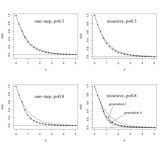
Figure 2: $\kappa^{+}_{i}(a)$ for forward tracing (one step, recursive tracing, $p=0.3$, and $p=0.8$, as indicated). Solid line: $\widehat{\kappa}(a)$, gray line: simulated data for generation 4 (if not indicated differently), dashed line: $\kappa^{+}_{i}(a)$ according to the theory for generation 4 (if not indicated differently), dots: first order approximation of $\kappa^{+}_{i}(a)$. Parameters: $\beta=2$, $\alpha=0.1$, $\sigma=0.9$, fixed tracing delay, $T=0.5$.

2.2.2 Special case: exponential delay

In order to compare fixed and random delay, we choose for $\phi(a)$ an exponential distribution with expectation $T$, $\phi(a)=e^{-a/T}/T$and obtain

$$\kappa_{i}(a)=\widehat{\kappa}(a)-\,p\,p_{\text{\text{obs}}}\,\widehat{\kappa}(a)\left(1-e^{-a/T}-\frac{\widehat{\kappa}(a)-e^{-a/T}}{1-T(\alpha+\sigma)}\right)+\mathcal{O}(p^{2}).$$

As before, the exponentially distributed delay induces a higher effect than the fixed delay (Figure 3).

2.2.3 Rates depending on age since infection

We again generalize the considerations above to the case that $\beta$, $\alpha$, and $\sigma$ depend on the time since infection. It is straight to obtain the equation for $\kappa_{i}(a)$, but unfortunately, the equations become even more unhandy as those above. However, a first order analysis in $p$ is possible and yields useful results.

The arguments completely parallel that of proposition 2.5. We find for $\kappa_{i}^{+}(a)$ the recursion formula

$$\kappa_{i-1}^{+}(b)\,\kappa_{i}(a|b) = \widetilde{\kappa}(a)\bigg{\{}\kappa_{i-1}^{+}(b)-p\,\int_{0}^{a}\left({-\kappa_{i-1}^{+}}^{\prime}(b+c)-\,\alpha(b+c)\,\kappa_{i-1}^{+}(b+c)\,\right)\,\int_{c}^{a}\phi(a^{\prime}-c)\,da^{\prime}\,dc\bigg{\}}$$

$$\kappa_{i}(a) = \frac{\int_{0}^{\infty}\kappa_{i}^{+}(a|b)\beta(b)\kappa_{i-1}^{+}(b)\,db}{\int_{0}^{\infty}\beta(\tau)\kappa_{i-1}^{+}(\tau)\,d\tau}$$

$$\widetilde{\kappa}(a) = e^{\int_{0}^{a}\,\sigma(\tau)+\alpha(\tau)\,d\tau}.$$

Figure 3: First order approximation of $\kappa^{\pm}(a)$ over $\widehat{\kappa}(a)$; left panel: backward-tracing, right panel: forward-tracing. Solid line: $\theta(a)=\delta_{T}(a)$, dashed line: $\phi(a)=e^{-a/T}/T$. Parameters: $\sigma=\alpha=1$, $p=0.3$, $\beta=3$, and $T=1$.

2.3 Full Tracing

Let $\kappa_{i}(a)$ denote the probability to be infectious at age of infection $a$. Its straight forward to combine forward and backward tracing, as we only need to repeat the argumentation of the last section, but taking into account that $\kappa_{0}(a)$ is for full tracing not given by $\kappa_{0}^{+}(a)=\exp(-(\alpha+\sigma)a)$, but by $\kappa_{-}(a)$. Hence we have the following result.

Proposition 2.7

We find for $\kappa_{0}(a)$ the

$$\kappa_{0}^{\prime}(a)=-\kappa_{0}(a)\left\{\alpha+\sigma+p\,\beta\,\left[(\phi\ast(1-\kappa_{0}))(a)-\alpha(\phi\ast\kappa_{0}^{\#})(a)\right]\right\},\quad\kappa_{0}(0)=1.$$ (6)

and for $\kappa_{i}(a)$ for $i>0$ the recursion formula

$$\kappa_{i-1}(b)\,\kappa_{i}(a|b) = \kappa_{0}(a)\bigg{\{}\kappa_{i-1}(b)-p\,\int_{0}^{a}\left({-\kappa_{i-1}}^{\prime}(b+c)-\,\alpha\,\kappa_{i-1}(b+c)\,\right)\,\int_{c}^{a}\phi(a^{\prime}-c)\,da^{\prime}\,dc\bigg{\}}$$ (7)

$$\kappa_{i}(a) = \frac{\int_{0}^{\infty}\kappa_{i}^{+}(a|b)\kappa_{i-1}(b)\,db}{\int_{0}^{\infty}\kappa_{i-1}(\tau)\,d\tau}.$$ (8)

These formulas are exact but not handy. For small tracing probabilities, however, a first order approximation is enough to estimate the effect of contact tracing. In order to do so we again only need to put together the results obtained for forward- and backward tracing.

Proposition 2.8

The first order approximation in $p$ reads

$$\kappa_{0}(a) = \widehat{\kappa}(a)\bigg{\{}1-p\,\,p_{\text{obs}}\,\,\beta\,\,(1\ast\phi\ast(1-\widehat{\kappa}))(a)\bigg{\}}+{\cal O}(p^{2}).$$ (9)

If $\int_{0}^{\varepsilon}\phi(a^{\prime})\,da^{\prime}\rightarrow 0$ for $\varepsilon\rightarrow 0$, then the first order approximation for $\kappa_{i}(a)$ is independent on $i$ (for $i>0$) and reads

$$\kappa_{i}(a) = \widehat{\kappa}(a)\bigg{\{}1-p\,\,p_{\text{obs}}\,\,\beta\,\,(1\ast\phi\ast(1-\widehat{\kappa}))(a)-\,\,p\,\,p_{\text{obs}}\,\,\big{(}\phi\ast(1-\widehat{\kappa})\big{)}(a)\bigg{\}}+{\cal O}(p^{2}).$$ (10)

Remark 2.9

The reproduction number in the $i$’th generation with contact tracing simply reads

$$R^{(i)}=\int_{0}^{\infty}\beta\kappa_{i}(a)\,da$$

$$= R_{0}-p\,\,p_{\text{obs}}\,\,\left\{\int_{0}^{\infty}\beta^{2}\,\,\widehat{\kappa}(a)\,\,(1\ast\phi\ast(1-\widehat{\kappa}))(a)\,da+\int_{0}^{\infty}\beta\widehat{\kappa}(a)\,\,\big{(}(1-\widehat{\kappa})\ast\phi\big{)}(a)\,da\right\}+{\cal O}(p^{2}).$$

In this approximation, the effects of forward- and backward tracing are clearly separated.

2.3.1 Fixed delay

As indicated, the first order approximation for $\kappa_{i}(a)$ is just a combination of the approximations for forward- and backward tracing. We obtain for $a<T$ that $\kappa_{i}(a)=\widehat{\kappa}(a)+{\cal O}(p^{2})$ and for $a>T$

$$\kappa_{-}(a)=e^{-(\alpha+\sigma)a}-p\,p_{\text{obs}}\,\,\,\widehat{\kappa}(a)\,\,\left\{\beta(a-T)-\frac{\beta}{\alpha+\sigma}\,\big{(}1-\widehat{\kappa}(a-T)\big{)}+(1-\widehat{\kappa}(a-T))\right\}+{\cal O}(p^{2}).$$

As before, numerical simulations indicate that the first order approximation is well suited as long as the probability is not too large (see figure 4).

We find

$$\int_{T}^{\infty}\hat{\kappa}(a)(1\ast\phi\ast(1-\widehat{\kappa}))(a)\,da = \widehat{\kappa}(T)\,\int_{T}^{\infty}\hat{\kappa}(a-T)\left\{(a-T)-\frac{1}{\alpha+\sigma}\,\left(1-e^{-(\alpha+\sigma)(a-T)}\right)\right\}\,da$$

$$= \frac{\widehat{\kappa}(T)}{2(\alpha+\sigma)^{2}}.$$

And, with $\phi\ast(1-\widehat{\kappa})(a)=(1-\widehat{\kappa}(a-T))$, we conclude that

$$\int_{T}^{\infty}\widehat{\kappa}(a)\,\,(\phi\ast(1-\widehat{\kappa}))(a)\,da = \widehat{\kappa}(T)\int_{0}^{\infty}\widehat{\kappa}(a)(1-\widehat{\kappa}(a))\,da=\frac{\widehat{\kappa}(T)}{2(\alpha+\sigma)}.$$

Hence, we obtain the following proposition.

Proposition 2.10

For a fixed delay, $\phi(a)=\delta_{T}(a)$, we obtain for $i>0$

$$R_{ct}:=R^{(i)}=R_{0}-\frac{1}{2}\,\,p\,p_{\text{obs}}\,\widehat{\kappa}(T)R_{0}(R_{0}+1)+{\cal O}(p^{2}).$$ (11)

The effect of contact tracing is (in first order of $p$) exponentially decreasing in the tracing delay. The time scale of this exponential decrease is given by the total removal rate $\gamma=\alpha+\sigma$.

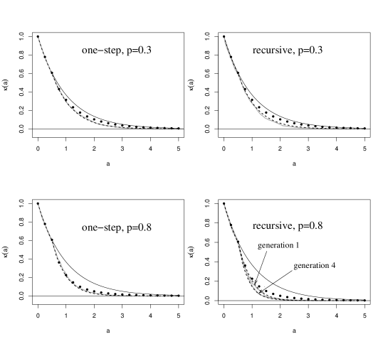
Figure 4: $\kappa_{i}(a)$ for full tracing (one step, recursive tracing, $p=0.3$, and $p=0.8$, as indicated). Solid line: $\widehat{\kappa}(a)$, gray line: simulated data for generation 4 (if not indicated differently), dashed line: $\kappa_{i}(a)$ according to the theory for generation 4 (if not indicated differently), dots: first order approximation of $\kappa_{i}(a)$.

2.3.2 Special case: exponential delay

We choose $\phi(a)=e^{-a/T}/T$. We do not state the first order approximation of $\kappa_{i}(a)$, as it is only necessary to combine the corresponding results from forward- and backward tracing. We focus on the first order effect of contact tracing on the reproduction number. The effect due to backward tracing is described by

$$\beta\int_{0}^{\infty}p\,p_{\text{obs}}\,\beta\,\widehat{\kappa}(a)\,\left\{a+T\,\,\,\frac{T(\alpha+\sigma)}{1-T(\sigma+\alpha)}\left((1-e^{-a/T})-\frac{1-\widehat{\kappa}(a)}{(T(\sigma+\alpha))^{2}}\right)\right\}\,da=\frac{p\,p_{\text{obs}}\,R_{0}^{2}}{2(1+T(\alpha+\sigma))}$$

and that for forward tracing

$$\beta\int_{0}^{\infty}\,p\,p_{\text{\text{obs}}}\,\widehat{\kappa}(a)\left(1-e^{-a/T}-\frac{\widehat{\kappa}(a)-e^{-a/T}}{1-T(\alpha+\sigma)}\right)\,da=\frac{p\,p_{\text{\text{obs}}}\,R_{0}\,}{2(1+T(\alpha+\sigma))}.$$

Proposition 2.11

For an exponentially distributed delay, $\phi(a)=e^{-a/T}/T$, we obtain for $i>0$

$$R_{ct}:=R^{(i)}=R_{0}-\frac{1}{2}\,\,p\,p_{\text{obs}}\,\frac{R_{0}(R_{0}+1)}{1+T(\alpha+\sigma)}+{\cal O}(p^{2}).$$ (12)

We again find that the exponential distributed delay yields a higher effect than the fixed delay (if we compare distributions with the same expectation). While the effect of the fixed delay decrease exponentially in $T$, the exponential delay only yields a polynomial decay. Indeed, $1/(1+T(\alpha+\sigma))$ is the [0/1]-Padé approximation of $\widehat{\kappa}(T)=\exp(-T(\alpha+\sigma))$. It is remarkable that in both cases, the effect of the delay only depends on $T(\alpha+\sigma)$, that is, on the quotient of the expected delay over the expected time of infection (in absence of contact tracing).

2.3.3 Rates depending on age since infection

To obtain the full model for the case if the rates depend on the age since infection, we again only have to combine forward- and backward tracing for this case. All in all, we obtain the equations for the probability to be infective at age of infection $a$ for an infected individual of the $i$’th generation $\kappa_{i}(a)$,

$$\kappa_{0}^{\prime}(a) = -\kappa_{0}(a)\bigg{(}\sigma(a)+\alpha(a)$$ (13)

$$\qquad\quad-p\,\int_{0}^{a}\phi(a-\tau)\int_{0}^{\tau}\bigg{(}\beta(c)\kappa^{\prime}_{0}(c)+\beta(c)\alpha(c)\kappa_{0}(c)\bigg{)}\,dc\,d\tau\bigg{)}$$

$$\kappa_{i-1}(b)\,\kappa_{i}(a|b) = \kappa_{0}(a)\bigg{\{}\kappa_{i-1}(b)$$ (14)

$$\qquad-p\,\int_{0}^{a}\left({-\kappa_{i-1}}^{\prime}(b+c)-\,\alpha(b+c)\,\kappa_{i-1}(b+c)\,\right)\,\int_{c}^{a}\phi(a^{\prime}-c)\,da^{\prime}\,dc\bigg{\}}$$

$$\kappa_{i}(a) = \frac{\int_{0}^{\infty}\kappa_{i}(a|b)\beta(b)\kappa_{i-1}(b)\,db}{\int_{0}^{\infty}\beta(\tau)\kappa_{i-1}(\tau)\,d\tau}.$$ (15)

2.3.4 Error analysis

We did focus on an approximate technique: though we are able to derive exact equations for $\kappa_{i}(a)$, these equations are too complex to be solved, and hence we basically focus on a first order approximation in the tracing probability $p$. However, in comparison with “real world epidemics” this is not the only simplification. The model itself is a simplification (SIS/SIR within an unstructured population), and also the branching process with tracing is only valid for the onset of the epidemic. Depletion of the class of susceptibles and tracing via contacts between infected individuals (no transmission of infection happen in these contacts) are neglected. Both effects gain importance if the disease approaches an endemic state.

Truncation error: In Figures 1 and 2, we compare simulations of the stochastic process resp. the numerical solution of the exact equations with the approximate solutions. For these simulations, the basic reproduction number $R_{0}=2$, and $p_{obs}=0.9$. While a reproduction of two is in an realistic range, the fraction of observed cases $p_{obs}=0.9$ is rather high to focus on the effect of contact tracing as well as to uncover potential approximation errors. We find by visual inspection that for reasonable tracing probabilities ($p$ below $0.3$, say), the agreement of our approximation and simulations is satisfying. Only if the tracing probability becomes larger ($p\approx 0.8$), the error is noticeable. Here, in particular the fraction of cases that become an index case $p_{obs}$ plays a role: if $p_{obs}$ is small, then even large tracing probabilities do not play a role.

Error due to the branching approximation: Reduction of the abundance of susceptibles due to the spread of the disease reduces the number of secondary cases, and in this, the number of infectious persons that can be detected by contact tracing. In order to have at least a heuristic method to deal this source of error, we propose to approximate what may be called the effective removal rate. This removal rate should induce in average the same mean infectious period as the stochastic process. Let us assume that the relative number of susceptibles is constant $u$ over a relatively long time period. The rate of infectious contacts is reduced from $\beta$ to $\beta\,u$. For a fixed delay, the effective reproduction number for a contact rate $\beta\,u$ is given by

$$R_{ct}\approx\frac{\beta u}{\alpha+\sigma}\left\{1-\frac{1}{2}\widehat{\kappa}(T)(\beta u/(\alpha+\sigma)+1)\right\}.$$

This, in turn, is equivalent with a mean recovery rate $\gamma=\gamma(u)$ given by

$$\gamma_{eff}(u)=\frac{\beta u}{R_{ct}}\approx\frac{\alpha+\sigma}{1-\frac{1}{2}\widehat{\kappa}(T)(\beta u/(\alpha+\sigma)+1)}.$$

We neglect in our considerations that also contacts between two infected persons take place. Also these contacts may lead to tracing events. However, if we compare stochastic simulations of the full epidemic process with contact tracing on the one hand, and a deterministic SIS-model with the nonlinear recovery rate given above, we find a satisfying agreement (see Fig. 5). The errors introduced by the saturation of the epidemic process are well met by the heuristic formula for the effective recovery rate given here.

Figure 5: Simulation of the stochastic (non-smooth line) and the approximate deterministic (smooth line) model. We use a fixed delay $T$, $\beta=2$, $\alpha=0.2$, $\sigma=0.9$, and recursive tracing. For $t<15$, $p=0$. At $t=15$ (indicated by the vertical solid line) $p$ is increased to $0.3$. The tracing delay is indicated by the difference between the dashed and the solid vertical line; at the solid line, contact tracing is introduced, at the dashed line, the first time tracing effects appear.

2.3.5 The interplay between tracing delay and latency period

The equation above is too complex to be directly useful in the sense that we obtain deeper inside into the interplay of the timing of the disease on the one hand, and tracing on the other hand. Therefore we concentrate on a special case: a fixed latency period $T_{i}$ and a fixed tracing delay $T$,

$$\beta(a)=\chi_{a>T_{i}}\,\beta,\quad\alpha(a)=\chi_{a>T_{i}}\,\alpha,\quad\sigma(a)=\chi_{a>T_{i}}\,\sigma,\quad\phi(a)=\delta_{T}(a)$$

where, as usual, $\chi_{a>T_{i}}$ denotes the characteristic function ($\chi_{a>T_{i}}=1$ if $a>T_{i}$ and $0$ else). We emphasize that $\beta(a)$ denotes a function, while $\beta$ is a constant (the same for $\alpha$ and $\sigma$). A first order approximation of the reproduction number is straightforward, but tedious; we move the computations to A, and only present the result here. Let $R_{ct}$ denote the reproduction number with contact tracing if the number of generations tends to infinity, and $R_{0}$ the reproduction number without contact tracing.

Corollary 2.12

$$R_{ct}=R_{0}-\frac{1}{2}\,\,p\,p_{\text{obs}}\,R_{0}\,\left[R_{0}\,\,\widehat{\kappa}(T+T_{i})+\frac{\widehat{\kappa}(\max(T_{i},T))}{\widehat{\kappa}(T_{i})}\,\,\left(2-\,\frac{\widehat{\kappa}(\max(T_{i},T))}{\widehat{\kappa}(T)}\right)\right]+{\cal O}(p^{2})$$ (16)

The tracing effect is monotonously decreasing in the tracing delay $T$. The first order effect consists of two parts, that for backward tracing (see Appendix A.1)

$$\frac{1}{2}\,\,p\,p_{\text{obs}}\,R_{0}^{2}\,\,\widehat{\kappa}(T+T_{i})$$

and that for forward tracing (see Appendix A.2)

$$\frac{1}{2}\,\,p\,p_{\text{obs}}\,R_{0}\,\,\frac{\widehat{\kappa}(\max(T_{i},T))}{\widehat{\kappa}(T_{i})}\,\,\left(2-\,\frac{\widehat{\kappa}(\max(T_{i},T))}{\widehat{\kappa}(T)}\right).$$

The backward tracing part is simply exponentially decreasing in the tracing delay and the latent period.

Figure 6: Strength of first order effect $R_{0}\,\,\widehat{\kappa}(T+T_{i})+\frac{\widehat{\kappa}(\max(T_{i},T))}{\widehat{\kappa}(T_{i})}\,\,\left(2-\,\frac{\widehat{\kappa}(\max(T_{i},T))}{\widehat{\kappa}(T)}\right)$ in dependency on $T$ and $T_{i}$ (measured in multiples of $1/(\alpha+\sigma)$, the mean infectious period) for $R_{0}=2$. Left panel: contour plot. Right panel: effect over $T$, $T_{i}$ fixed at indicated values.

The dependency of the froward tracing effect on tracing delay resp. latent period is more complex. First of all, we find that for $T_{i}=T$, the two delays in the forward effect cancel each other: There is a race between tracing and infection. If both mechanisms are subject to the same delay, the effects of the delays do cancel. If $T<T_{i}$, the forward tracing effect is even larger than that without any delay; only if $T>T_{i}$, the effect decreases exponentially in $T$.

In order to compare the relative importance of forward- and backward tracing, we distinguish the cases $T>T_{i}$ and $T<T_{i}$.
Case $T>T_{i}$:

$$R_{ct}=R_{0}-\frac{1}{2}\,\,p\,p_{\text{obs}}\,R_{0}\,\widehat{\kappa}(T+T_{i}))\bigg{[}R_{0}\,\,+1\,\bigg{]}+{\cal O}(p^{2})$$

As the backward term incorporates $R_{0}$, and the forward term $1$, the backward tracing will contribute considerable more to the (first order) tracing effect.

Case $T<T_{i}$:

$$R_{ct}=R_{0}-\frac{1}{2}\,\,p\,p_{\text{obs}}\,R_{0}\,\widehat{\kappa}(T+T_{i})\,\left[R_{0}\,\,+\frac{2-\,\widehat{\kappa}(T_{i}-T)}{\widehat{\kappa}(T+T_{i})}\right]+{\cal O}(p^{2})$$

This time we compare $R_{0}$ with $(2-\widehat{\kappa}(T_{i}-T))/\widehat{\kappa}(T_{i}+T)$. In principle, the latter term can be arbitrarily large, in particular if $T_{i}$ is large and $T$ small; note that $(2-\widehat{\kappa}(T_{i}-T))/\widehat{\kappa}(T_{i}+T)$ is always increasing in $T_{i}$ (for $T$ fixed). For long latency periods and small tracing delays, forward tracing gains increasingly importance. Forward tracing benefits from a long latency period.

If we fix $T_{i}$, the first order effect is simply decreasing in $T$. If $T_{i}$ is rather large, a small tracing delay affects the effect only weakly (see Fig. 6); only if the latency period is small or the tracing delay is in the same magnitude (or larger) than the latency period, the delay in the tracing process strongly decreases the effect.
If $T$ is fixed, then the effect is in general non-monotonously in $T_{i}$: If $T$ is below a certain value, the effect is simply decreasing in $T_{i}$, if $T$ is above this value, the effect is in a first interval decreasing, but eventually increasing in $T_{i}$. The reason for this observation is based on the effect that we observe the sum of forward- and backward tracing. Backward tracing is always decreasing in $T_{i}$ if $T$ is fixed. Forward tracing, however, is decreasing if $T_{i}<T$, but increasing for $T_{i}>T$. If the impact of forward tracing is large enough, a non-monotone effect (in $T_{i}$) may appear.

3 Discussion

In the present work, we continued the investigations of Ball et al. [2, 3] about tracing delays, taking into account forward- and backward tracing. This study particularly focused on the questions how randomness in the tracing delay affects the effect of contact tracing to fight an epidemic during the initial phase of an outbreak, if forward- or backward tracing plays a more decisive role, and how the interplay between the time scales involved influences contact tracing. With respect to the last question, we focused on the mean tracing delay on the one hand, and the average time of infection (without control measure) respectively a latent period.

In order to approach these questions, we focused on the onset of an epidemic, and used a branching process approximation for the spread of infections. On top of this linear branching process, contact tracing has been introduced. The tracing leads to dependencies between individuals, which makes the stochastic process more complex to analyze analytically. The main tool to analyze the process is the probability for an infected individual to be still infectious at a given age of infection. It has been possible to derive a system of integro-differential equations for this probability. As an explicit solution seems to be difficult to obtain, approximate solutions (for small tracing probability) have been derived. Based upon these approximations, an approximation for the reproduction number has been proposed.

The present study addressed the effect of randomness in the tracing delay: If we compare a fixed and an exponentially distributed tracing delay, we find that the effect of the fixed delay is smaller than that of the exponential distribution (if both have the same expectation). Most likely, the main reason for this observation is the exponential decrease of the probability to be infected at a certain age of infection: The expected number of infections produced after a certain age of infection will decrease exponentially (note that we do not condition on the fact that a person reaches this age of infection). In a situation with randomness in the delay, some persons are detected earlier, and some later in comparison with the fixed delay. Due to the exponential decrease, the gain in the effect by the more early detections is higher than the loss in effect by the later detections. This difference leads to an exponential respectively a polynomial decrease of the effect on the mean tracing delay. This finding may underline the importance to avoid outliers in the tracing delay: if the time between detection of an index case and investigation of contacts becomes large, contact tracing for this index case becomes inefficient. The efficiency of tracing for one index case does not decrease linearly in the tracing delay, but exponentially. Considering the high costs for contact tracing, it may be worth to implement a tracing program in such a way that a long tracing delay for an index cases is not likely to occur. However, a delay becomes notable only if it is in the range of the infectious period, as it is to expect. If it is distinctively shorter, the delay hardly plays a role, if it is longer, contact tracing becomes inefficient.

If we introduce a latency period, we find the same result for backward tracing (and a deterministic, fixed delay) as before: the effect decreases exponentially, where the ratio between tracing delay and latency period (delay in infectivity) is decisive. It is slightly different in forward tracing: here, the effect is even stronger compared with the case without any delay (no tracing delay and no latency period) if the tracing delay is shorter than the latency period. We clearly find a race between forward tracing and infections. Only if the tracing delay becomes larger than the latency period, we again find an exponential decrease in the effect. Forward tracing benefits from a long latency period, and may even become stronger than backward tracing. If the tracing- and the latency period are in the same range, backward tracing is more likely to play the central role.

Basically, we have three ingredients of the implementation of a contact tracing program that decide about its efficiency: (a) the probability for an infectious person to become an index case (b) how likely is a contact reported by an index case and (c) how large is the tracing delay. At lowest order, the effect (measured by the reproduction number) is the product of the first two probabilities times an exponentially decreasing function in the tracing delay. The time scale of this decrease is given by the recovery rate, and affected by the latency period. One may think about resource allocation within a tracing program. As long as the tracing delay is distinctively shorter than the latency period resp. the infectious period, it seems to be better to put effort in the detection of more contacts or index cases. Only if the disease is fast (short latency period/infectious period), it is of importance to decrease the tracing delay. If, however, the time scale of the infection is too fast, contact tracing as a control measure could be inadequate. These findings are in line with, e.g., results by Fraser et al. [8]

Appendix A Latency period

We aim at a first order approximation (the only analysis that is feasible in general); we find

$$\kappa_{0}^{\prime}(a) = -\kappa_{0}(a)\bigg{(}\sigma(a)+\alpha(a)$$

$$\qquad\quad-p\,\int_{0}^{a}\phi(a-\tau)\int_{0}^{\tau}\bigg{(}\beta(c)\widetilde{\kappa}^{\prime}(c)+\beta(c)\alpha(c)\widetilde{\kappa}(c)\bigg{)}\,dc\,d\tau\bigg{)}+{\cal O}(p^{2})$$

$$\kappa_{i-1}(b)\,\kappa_{i}(a|b) = \kappa_{0}(a)\bigg{\{}\kappa_{i-1}(b)$$

$$\qquad-p\,\int_{0}^{a}\left({-\widetilde{\kappa}}^{\prime}(b+c)-\,\alpha(b+c)\,\widetilde{\kappa}(b+c)\,\right)\,\int_{c}^{a}\phi(a^{\prime}-c)\,da^{\prime}\,dc\bigg{\}}+{\cal O}(p^{2})$$

$$\kappa_{i}(a) = \frac{\int_{0}^{\infty}\kappa_{i}(a|b)\beta(b)\kappa_{i-1}(b)\,db}{\int_{0}^{\infty}\beta(\tau)\kappa_{i-1}(\tau)\,d\tau}$$

$$\widetilde{\kappa}(a) = e^{\int_{0}^{a}\,\sigma(\tau)+\alpha(\tau)\,d\tau}.$$

Proposition A.1

Up to second order in $p$, $\kappa_{i}(a)=\kappa_{1}(a)$ for $i>0$.

Proof: We first find

$$\kappa_{i}(a|b)$$ (17)

$$= \kappa_{0}(a)\bigg{\{}1-\frac{p}{\kappa_{i-1}(b)}\,\int_{0}^{a}\left({-\widetilde{\kappa}}^{\prime}(b+c)-\,\alpha(b+c)\,\widetilde{\kappa}(b+c)\,\right)\,\int_{c}^{a}\phi(a^{\prime}-c)\,da^{\prime}\,dc\bigg{\}}+{\cal O}(p^{2})$$

$$= \kappa_{0}(a)\bigg{\{}1-p\,\int_{0}^{a}\,\,\,\left(\frac{{-\widetilde{\kappa}}^{\prime}(b+c)}{\widetilde{\kappa}(b)}-\,\alpha(b+c)\,\frac{\widetilde{\kappa}(b+c)}{\widetilde{\kappa}(b)}\,\right)\,\int_{c}^{a}\phi(a^{\prime}-c)\,da^{\prime}\,\,\,dc\bigg{\}}+{\cal O}(p^{2})$$

and hence $\kappa_{i}(a|b)=\kappa_{1}(a|b)+{\cal O}(p^{2})$. We drop the index and simply write $\kappa(a|b)=\kappa_{1}(a|b)+{\cal O}(p^{2})$, where $\kappa(a|b)$ is defined by equation (17), where the ${\cal O}(p^{2})$ terms are neglected. In zero order, $\kappa_{0}(a)=\widetilde{\kappa}(a)$, and hence also $\kappa(a|b)=\widetilde{\kappa}(a)$; we write

$$\kappa(a|b)=\widetilde{\kappa}(a)+p\zeta(a|b)$$

where $\zeta(a|b)$ does not depend on $p$. Hence,

$$\kappa_{i}(a) = \frac{\int_{0}^{\infty}\big{(}\widetilde{\kappa}(a)+p\zeta(a|b)\big{)}\beta(b)\kappa_{i-1}(b)\,db}{\int_{0}^{\infty}\beta(\tau)\kappa_{i-1}(\tau)\,d\tau}+{\cal O}(p^{2})=\widetilde{\kappa}(a)+p\,\frac{\int_{0}^{\infty}\zeta(a|b)\beta(b)\kappa_{i-1}(b)\,db}{\int_{0}^{\infty}\beta(\tau)\kappa_{i-1}(\tau)\,d\tau}+{\cal O}(p^{2})$$

$$= \widetilde{\kappa}(a)+p\,\frac{\int_{0}^{\infty}\zeta(a|b)\beta(b)\widetilde{\kappa}(b)\,db}{\int_{0}^{\infty}\beta(\tau)\widetilde{\kappa}(\tau)\,d\tau}+{\cal O}(p^{2}).$$

As a consequence, the first order correction of the asymptotic reproduction number ($i\rightarrow\infty$) consist of two clearly separated parts: that due to forward tracing, and that due to backward tracing. Note that we choose the signs in the definition of $\eta_{\pm}$ below in such a way, that the correction terms of the reproduction number have a minus sign.

Proposition A.2

Let $\kappa_{0}(a)=\widetilde{\kappa}(a)-p\eta_{-}(a)+{\cal O}(p^{2})$,

$$\eta_{+}(a)=\widetilde{\kappa}(a)\frac{\int_{0}^{\infty}\int_{0}^{a}\,\,\,\left(\frac{{-\widetilde{\kappa}}^{\prime}(b+c)}{\widetilde{\kappa}(b)}-\,\alpha(b+c)\,\frac{\widetilde{\kappa}(b+c)}{\widetilde{\kappa}(b)}\,\right)\,\int_{c}^{a}\phi(a^{\prime}-c)\,da^{\prime}\,dc\,\,\beta(b)\widetilde{\kappa}(b)\,db}{\int_{0}^{\infty}\beta(\tau)\widetilde{\kappa}(\tau)\,d\tau}$$

$r_{\pm}=\int_{0}^{\infty}\beta(a)\,\eta_{\pm}(a)\,da$. Then,

$$R_{ct}=R_{0}-p(r_{+}+r_{-})+{\cal O}(p^{2}).$$

This proposition is a direct consequence of equ. (17).

Now we specify the parameters as indicated above: $\beta(a)$, $\alpha(a)$ and $\sigma(a)=0$ for $a<t_{i}$, and are constant ($\beta$, $\alpha$, $\sigma$) afterwards; The contact tracing delay is a constant $T$. We compute the reproduction number and the first order correction terms for $R_{ct}$. We will use

$$\widehat{\kappa}(a)=e^{-(\alpha+\sigma)\,a},\quad\widetilde{\kappa}(a)=e^{-\int_{0}^{a}(\alpha(\tau)+\sigma(\tau))\,d\tau}$$

such that $\widetilde{\kappa}(a)=\widehat{\kappa}(a-T_{i})$ for $a>T_{i}$. The zero order term is a direct consequence of $R_{0}=\int_{0}^{\infty}\beta(a)\,\widetilde{\kappa}(a)\,da$.

Proposition A.3

$R_{0}=\frac{\beta}{\alpha+\sigma}$.

A.1 First order approximation: backward tracing

Proposition A.4

The first order approximation reads

$$\kappa_{0}(a)=\widehat{\kappa}(a)+{\cal O}(p^{2})\quad\mbox{for}\quad a\leq T_{i}+T_{t}.$$

and for $a>T_{i}+T$

$$\kappa_{0}(a) = \widehat{\kappa}(a)\,\,\left[1-p\,\beta\,p_{\text{obs}}\,\left((a-T_{i}-T)-\frac{1}{\alpha+\sigma}(1-\widetilde{\kappa}(a-T-T_{i})\right)\right]+{\cal O}(p^{2})$$

Proof: The proof consist of direct computations.

$$\kappa_{-}^{\prime}(a) = -\kappa_{-}(a)\left(\sigma(a)+\alpha(a)-p\,\int_{0}^{a}\phi(a-\tau)\int_{0}^{\tau}\bigg{(}\beta(\tau-c)\widetilde{\kappa}^{\prime}(c)+\beta(\tau-c)\alpha(c)\widetilde{\kappa}(c)\bigg{)}\,dc\,d\tau\right)+{\cal O}(p^{2})$$

$$= -\kappa_{-}(a)\left(\sigma(a)+\alpha(a)-p\,\int_{0}^{a}\phi(a-\tau)\int_{0}^{\tau-T_{i}}\bigg{(}\beta\sigma(c)\widetilde{\kappa}(c)\bigg{)}\,dc\,\chi_{\tau>T_{i}}\,d\tau\right)+{\cal O}(p^{2})$$

$$= -\kappa_{-}(a)\left((\sigma+\alpha)\,\,\chi_{a>T_{i}}+p\,\beta\,\sigma\,\int_{0}^{a}\phi(a-\tau)\int_{T_{i}}^{\tau-T_{i}}e^{(\alpha+\sigma)(c-T_{i})}\,dc\,\,\,\chi_{\tau>2\,T_{i}}\,d\tau\right)+{\cal O}(p^{2})$$

$$= -\kappa_{-}(a)\left(\sigma(a)+\alpha(a)+p\,\beta\,p_{\text{obs}}\,\int_{0}^{a}\phi(a-\tau)\,\left(1-\widehat{\kappa}(\tau-2\,T_{i})\right)\,\,\chi_{\tau>2T_{i}}\,d\tau\right)+{\cal O}(p^{2})$$

$$= -\kappa_{-}(a)\bigg{(}\sigma(a)+\alpha(a)+p\,\beta\,p_{\text{obs}}\,\left(1-\widehat{\kappa}(a-T-2\,T_{i})\right)\,\,\chi_{a>2\,T_{i}+T}\bigg{)}\,+{\cal O}(p^{2})$$

where we used the definition $\widehat{\kappa}(a)=e^{-(\alpha+\sigma)a}$ for $a>0$. Then,

$$\kappa_{-}(a) = \widehat{\kappa}(a)\,\,e^{\chi_{a>2\,T_{i}+T}\,p\,\beta\,p_{\text{obs}}\,\left((a-2\,T_{i}-T)-\frac{1}{\alpha+\sigma}(1-\widehat{\kappa}_{-}(a-T-T_{i}))\right)}+{\cal O}(p^{2})$$

$$= \widetilde{\kappa}(a)\,\,\left[1-p\,\beta\,p_{\text{obs}}\,\chi_{a>2\,T_{i}+T}\,\left((a-2\,T_{i}-T)-\frac{1}{\alpha+\sigma}(1-\widetilde{\kappa}_{-}(a-T-2\,T_{i}))\right)\right]+{\cal O}(p^{2})$$

The term $2\,T_{i}$ is a consequence of backward tracing: An infectee is only produced after $T_{i}$ time units, and the earliest time point at which this infectee can be observed is $T_{i}$ time units after his/her infection. Hence, the earliest time point at which a backward tracing event can be triggered is $2T_{i}$, and the infector is then traced at age of infection $2\,T_{i}+T$.

Consequently, we have (note our sign convention)

$$\eta_{-}(a)=\widetilde{\kappa}(a)\,\,\,\beta\,p_{\text{obs}}\,\chi_{a>2\,T_{i}+T}\,\left((a-2\,T_{i}-T)-\frac{1}{\alpha+\sigma}(1-\widehat{\kappa}(a-T-2\,T_{i}))\right).$$

Evaluating the integral $r_{-}=\int_{0}^{\infty}\beta(a)\,\eta_{-}(a)\,da$ yields

$$r_{-}=\frac{1}{2}\,\,p_{\text{obs}}\,\,R_{0}^{2}\,\,\,\widehat{\kappa}(T+T_{i}).$$ (18)

A.2 First order approximation: forward tracing

Proposition A.5

$\eta_{+}(a)=p_{\text{obs}}\,\,\chi_{a>T}\,\,\widetilde{\kappa}(a)(1-\widehat{\kappa}(a-T)).$

Proof: We evaluate

$$\eta_{+}(a)=\widetilde{\kappa}(a)\frac{\int_{0}^{\infty}\int_{0}^{a}\,\,\,\left(\frac{{-\widetilde{\kappa}}^{\prime}(b+c)}{\widetilde{\kappa}(b)}-\,\alpha(b+c)\,\frac{\widetilde{\kappa}(b+c)}{\widetilde{\kappa}(b)}\,\right)\,\int_{c}^{a}\phi(a^{\prime}-c)\,da^{\prime}\,dc\,\,\beta(b)\widetilde{\kappa}(b)\,db}{\int_{0}^{\infty}\beta(\tau)\widetilde{\kappa}(\tau)\,d\tau}$$

which yields the result for our special case as $\int_{0}^{\infty}\beta(\tau)\widetilde{\kappa}(\tau)\,d\tau=R_{0},$ $\int_{c}^{a}\phi(a^{\prime}-c)\,da^{\prime}=\chi_{a>T}\,\,\chi_{c<a-T}$, and

$$\left(\frac{{-\widetilde{\kappa}}^{\prime}(b+c)}{\widetilde{\kappa}(b)}-\,\alpha(b+c)\,\frac{\widetilde{\kappa}(b+c)}{\widetilde{\kappa}(b)}\,\right)=\sigma(b+c)\,\frac{\widetilde{\kappa}(b+c)}{\widetilde{\kappa}(b)}.$$

Note that the out-most integral only extends over $b\in[T_{i},\infty)$ as $\beta(b)=0$ for $b<T_{i}$. For $b>T_{i}$, we have

$$\sigma(b+c)\,\widetilde{\kappa}(b+c)/\widetilde{\kappa}(b)=\sigma\,\widehat{\kappa}(b+c-T_{i})/\widehat{\kappa}(b-T_{i})=\sigma\,\widehat{\kappa}(c).$$

That is, the inner integral does not depend on $b$, and the result follows easily.

Integrating $\beta(a)\,\eta_{+}(a)$ over $a\in\mathbb{R}_{+}$ yields the correction term for forward tracing,

$$r_{+} = \frac{1}{2}\,\,p_{\text{obs}}R_{0}\,\,\widehat{\kappa}(\max(T_{i},T)-T_{i})\,\,\bigg{(}2-\,\,\widehat{\kappa}(\max(T_{i},T)-T)\bigg{)}$$ (19)

$$= \frac{1}{2}\,\,p_{\text{obs}}R_{0}\,\,\frac{\widehat{\kappa}(\max(T_{i},T))}{\widehat{\kappa}(T_{i})}\,\,\bigg{(}2-\,\,\frac{\widehat{\kappa}(\max(T_{i},T))}{\widehat{\kappa}(T)}\bigg{)}.$$

References

- [1] F. Ball and P. Donnelly. Strong approximations for epidemic models. Stoch. Proc. Appl., 55:1–21, 1995.
- [2] F. G. Ball, E. S. Knock, and P. D. O’Neill. Threshold behaviour of emerging epidemics featuring contact tracing. Adv. in Appl. Probab., 43:1048–1065, 12 2011.
- [3] F. G. Ball, E. S. Knock, and P. D. O’Neill. Stochastic epidemic models featuring contact tracing with delays. Mathematical Biosciences, 266:23 – 35, 2015.
- [4] M. Begun, A. T. Newall, G. B. Marks, and J. G. Wood. Contact tracing of tuberculosis: A systematic review of transmission modelling studies. PLoS ONE, 8(9):e72470, 2013.
- [5] K. T. Eames and M. J. Keeling. Modeling dynamic and network heterogeneities in the spread of sexually transmitted diseases. PNAS, 99:13330 – 13335, 2002.
- [6] M. Eichner. Case isolation and contact tracing can prevent the spread of smallpox. American Journal of Epidemiology, 158:118–128, 2003.
- [7] G. Fox, N. Nhung, D. Sy, W. Britton, and G. Marks. Household contact investigation for tuberculosis in Vietnam: study protocol for a cluster randomized controlled trial. Trials, 14:342, 2013.
- [8] C. Fraser, S. Riley, R. Anderson, and N. Ferguson. Factors that make an infectious disease outbreak controllable. PNAS, 101:6146 – 6151, 2004.
- [9] H. W. Hethcote and J. A. Yorke. Gonorrhea transmission dynamics and control. Lecture Notes in Biomathematics, 56, 1984.
- [10] T. House and M. J. Keeling. The impact of contact tracing in clustered populations. PLoS Comput Biol, 6:e1000721, 2010.
- [11] M. Keeling. Correlation equations for endemic diseases. Proc. Roy. Soc. Lond. B, 266:953–961, 1999.
- [12] I. Z. Kiss, D. M. Green, and R. R. Kao. Infectious disease control using contact tracing in random and scale-free networks. J. R. Soc. Interface, 3:55–62, 2006.
- [13] I. Z. Kiss, D. M. Green, and R. R. Kao. The effect of network mixing patterns on epidemic dynamics and the efficacy of disease contact tracing. J. R. Soc. Interface, 5:791–799, 2008.
- [14] D. Klinkenberg, C. Fraser, and H. Heesterbeek. The effectiveness of contact tracing in emerging epidemics. PLoS ONE, 1:e12, 2006.
- [15] J. Müller and V. Hösel. Estimating the tracing probability from contact history at the onset of an epidemic. Math. pop. Stud., 14:211–236, 2007.
- [16] J. Müller, M. Kretzschmar, and K. Dietz. Contact tracing in stochastic and deterministic epidemic models. Mathematical Biosciences, 164:39 – 64, 2000.
- [17] J. Müller and M. Möhle. Family trees of continuous-time birth-and-death processes. J. Appl. Probab., 40:980–994, 12 2003.
- [18] C. Rivers, E. Lofgren, M. Marathe, S. Eubank, and B. Lewis. Modeling the impact of interventions on an epidemic of Ebola in Sierra Leone and Liberia. PLOS Currents Outbreaks, Edition 2, 2014.
- [19] N. Shaban, M. Andersson, Åke Svensson, and T. Britton. Networks, epidemics and vaccination through contact tracing. Mathematical Biosciences, 216:1 – 8, 2008.
- [20] H. Stoddart and N. Noah. Usefulness of screening large numbers of contacts for tuberculosis: questionnaire based review. BMJ, 315:651, 197.