A class of Weiss-Weinstein bounds and its relationship with the Bobrovsky-Mayer-Wolf-Zakaï bounds

Abstract

A fairly general class of Bayesian ”large-error” lower bounds of the Weiss-Weinstein family, essentially free from regularity conditions on the probability density functions support, and for which a limiting form yields a generalized Bayesian Cramér-Rao bound (BCRB), is introduced. In a large number of cases, the generalized BCRB appears to be the Bobrovsky-Mayer-Wolf-Zakai bound (BMZB). Interestingly enough, a regularized form of the Bobrovsky-Zakai bound (BZB), applicable when the support of the prior is a constrained parameter set, is obtained. Modified Weiss-Weinstein bound and BZB which limiting form is the BMZB are proposed, in expectation of an increased tightness in the threshold region. Some of the proposed results are exemplified with a reference problem in signal processing: the Gaussian observation model with parameterized mean and uniform prior.

I Introduction

Under the mean square error (MSE) criterion, the mean of the a posteriori probability density function (pdf) of a random parameter, conditioned on the observed data, is the optimal solution to the parameter estimation problem. However, except for a few special cases, determining the posterior mean is computationally prohibitive, and various approaches have been developed as alternatives. It is therefore of interest to determine the degradation in accuracy resulting from the use of suboptimal methods [1][2]. Unfortunately again, the computation of the MSE of the conditional mean estimator generally requires multiple integration, a computationally intensive task [1][2]. This has led to a large body of work [3][4][5] seeking to find both computationally tractable and tight Bayesian lower bounds (BLBs) on the attainable MSE to which the performance of the optimal estimator or any suboptimal estimation scheme can be compared.

Historically, computational tractability and ease of use seem to have been the prominent qualities requested for a lower bound, as exemplified by the Bayesian Cramér-Rao bound (BCRB), the first Bayesian lower bound to be derived [6][7], and still the most commonly used BLB. Nevertheless, it is now well known that the BCRB is an optimistic bound in a non-linear estimation problem where the outliers effect generally appears, leading to a characteristic behavior of estimators MSE which exhibits three distinct regions of operation depending on the number of (independent) observations and/or on the signal to noise ratio (SNR) [3]. More precisely, at high SNR and/or for a high number of observations, i.e., in the asymptotic region, the outliers effect can be neglected and the ultimate performance are generally described by the BCRB. However, when the SNR and/or the number of observations decrease, the outliers effect leads to a quick increase of the MSE: this is the so-called threshold effect which is not predicted by the BCRB. Finally, at low SNR and/or at low number of observations, the observations provide little information, and the MSE is close to that obtained from the prior knowledge about the problem yielding the no-information region.

Therefore after computational tractability, tightness and/or relaxation of some regularity assumptions on the problem setting [8][9][10][11] have become the prominent qualities looked for a lower bound in non-linear estimation problems. Indeed, from a practical point of view, the knowledge of the particular value for which the threshold effect appears is a key feature allowing to define estimators optimal operating area. This has led to a large body of research based, so far, on two main families, i) the Ziv-Zakai family (ZZF) resulting from the conversion of an estimation bounding problem into one bounding binary hypothesis testing [8][9][12] and, ii) the Weiss-Weinstein family (WWF), derived from a covariance inequality principle [5][6][7][10][11][13][14][15][17][16]. In each family, some bounds, generally called ”large-error” bounds (in contrast with ”small-error” bounds such as the BCRB), can predict the threshold effect [3].

In the present paper we focus on the Weiss-Weinstein family. The main contribution of the paper is to introduce a fairly general class of ”large-error” bounds of the WWF essentially free from regularity conditions and for which a limiting form yields a generalized BCRB. Indeed, within this class of lower bounds, the supports of the joint and conditional pdfs must only be a countable union of disjoint non empty intervals of $\mathbb{R}$ (which naturally includes connected or disconnected subsets of $\mathbb{R}$, bounded or unbounded intervals) and the bound-generating functions must only have a finite second order moment. Additionally, we provide (Propositions 1 and 2) some mild regularity conditions in order to obtain a non trivial limiting form (non zero generalized BCRB) of the ”large-error” bound considered. In a large number of cases, this limiting form appears to be the Bobrovsky-Mayer-Wolf-Zakai bound (BMZB) [14]. Therefore, the proposed class of Bayesian lower bounds defines a wide range of Bayesian estimation problems for which a non trivial generalized BCRB exists, which is a key result from a practical viewpoint. Indeed, the computational cost of large-error bounds is prohibitive in most applications when the number of unknown parameters increases.
Interestingly enough, the proposed class of lower bounds provides the expression of all existing bounds of the WWF mentioned in [4] and [5] when the pdfs support is a constrained parameter set, including a regularized form of the Bobrovsky-Zakai bound (BZB) [10]. From a practical viewpoint, it is another noticeable result, since the BZB is the easiest to use ”large-error” bound, but was believed to be inapplicable in that case [10, Section II][11, p682][13, p340][3, p39].
Last, as a by-product, since the BMZB may provide a tighter bound than the historical BCRB in the asymptotic region [14][3, p36], it would seem sensible to introduce modified Weiss-Weinstein bound (WWB) and BZB which limiting form is the BMZB, in expectation of an increased tightness in the threshold region as well.

Some of the proposed results are exemplified with a reference problem in signal processing: the Gaussian observation model with parameterized mean depending on a random parameter with uniform prior. For numerical evaluations, we focus on the estimation of a single tone.

For sake of legibility, we only discuss in details the case of a single random parameter. Extension of the proposed results to a vector of parameters can be done by resorting to the covariance matrix inequality as shown in [13, p341][14, p1429].

II A new class of Bayesian lower bounds of the Weiss-Weinstein family

Throughout the present paper scalars, vectors and matrices are represented, respectively, by italic (as in $a$ or $A$), bold lowercase (as in $\mathbf{a}$) and bold uppercase (as in $\mathbf{A}$) characters. The $n$-th row and $m$-th column element of the matrix $\mathbf{A}$ is denoted by $\left\{\mathbf{A}\right\}_{n,m}$, whereas, $\left\{\mathbf{a}\right\}_{n}$ represents the $n$-th coordinate of the column vector $\mathbf{a}$. The real and imaginary part of $A$, are denoted, respectively, by $\mathop{\mathrm{R}e}\left\{A\right\}$ and $\mathop{\mathrm{I}m}\left\{A\right\}$. The transpose, transpose conjugate operator are indicated, respectively, by $.^{T}$ and $.^{H}$. The identity matrix of size $M$ is denoted by $\mathbf{I}_{M}$. For any given two matrices $\mathbf{A}$ and $\mathbf{B}$, $\mathbf{A}\succeq\mathbf{B}$ means that $\mathbf{A}-\mathbf{B}$ is positive semi-definite matrix. $E\left[.\right]$ denotes the expectation operator and $1_{A}\left(\mathbf{x}\right)$ is the indicator function of subset $A$ of $\mathbb{R}^{N}$.

II-A Definitions and Assumptions

Throughout the present paper:

• $\mathbf{x}$ denotes a $N$-dimensional complex random observation vector belonging to the observation space $\mathcal{X}\subset\mathbb{C}^{N}$.

• $\theta$ denotes a real random parameter belonging to the parameter space $\Theta\subset\mathbb{R}$.

• $\mathcal{S}_{\mathcal{X},\Theta}\subset\mathbb{C}^{N}\times\mathbb{R}$ denotes the support of the the joint pdf $p\left(\mathbf{x},\theta\right)$ of $\mathbf{x}$ and $\theta$ such that $\mathcal{S}_{\mathcal{X},\Theta}=\left\{\left(\mathbf{x}^{T},\theta\right)^{T}\in\mathbb{C}^{N}\times\mathbb{R}\text{ : }p\left(\mathbf{x},\theta\right)>0\right\}$.

• $\mathcal{S}_{\Theta}\subset\mathbb{R}$ denotes the support of the prior pdf of $\theta$ denoted $p\left(\theta\right)$, i.e., $\mathcal{S}_{\Theta}=\left\{\theta\in\mathbb{R}:p\left(\theta\right)>0\right\}$.

• $\mathcal{S}_{\mathcal{X}}\subset\mathbb{C}^{N}$ denotes the support of the marginal pdf of $\mathbf{x}$ denoted $p\left(\mathbf{x}\right)$, i.e., $\mathcal{S}_{\mathcal{X}}=\left\{\mathbf{x}\in\mathbb{C}^{N}:p\left(\mathbf{x}\right)>0\right\}$.

• Furthermore, $\forall\mathbf{x}\in\mathcal{S}_{\mathcal{X}}$, let us denote $\mathcal{S}_{\Theta|\mathbf{x}}=\left\{\theta\in\mathbb{R}:p\left(\mathbf{x},\theta\right)>0\right\}$ and $\forall\theta\in\mathcal{S}_{\Theta}$, $\mathcal{S}_{\mathcal{X}|\theta}=\left\{\mathbf{x}\in\mathbb{C}^{N}:p\left(\mathbf{x},\theta\right)>0\right\}$. Then:

  $$p\left(\theta\right)=\mathop{\displaystyle\int}\limits_{\mathbb{C}^{N}}p\left(\mathbf{x},\theta\right)1_{\mathcal{S}_{\mathcal{X}|\theta}}\left(\mathbf{x}\right)d\mathbf{x}=\mathop{\displaystyle\int}\limits_{\mathcal{S}_{\mathcal{X}|\theta}}p\left(\mathbf{x},\theta\right)d\mathbf{x,\quad}p\left(\mathbf{x}\right)=\mathop{\displaystyle\int}\limits_{\mathbb{R}}p\left(\mathbf{x},\theta\right)1_{\mathcal{S}_{\mathbf{\Theta}|\mathbf{x}}}\left(\mathbf{x}\right)d\theta=\mathop{\displaystyle\int}\limits_{\mathcal{S}_{\Theta|\mathbf{x}}}p\left(\mathbf{x},\theta\right)d\theta.$$

Thus, for a given function $f:\mathcal{X}\times\Theta\rightarrow\mathbb{R}$, deterministic, unknown and measurable function, one has:

$$E_{\mathbf{x},\theta}\left[f\left(\mathbf{x},\theta\right)\right] = \mathop{\displaystyle\int}\limits_{\mathbb{C}^{N}}\mathop{\displaystyle\int}\limits_{\mathbb{R}}f\left(\mathbf{x},\theta\right)p\left(\mathbf{x},\theta\right)1_{\mathcal{S}_{\mathcal{X},\Theta}}(\mathbf{x},\theta)d\mathbf{x}d\theta=\mathop{\displaystyle\int}\limits_{\mathcal{S}_{\mathcal{X}}}\mathop{\displaystyle\int}\limits_{\mathcal{S}_{\Theta|\mathbf{x}}}f\left(\mathbf{x},\theta\right)p\left(\mathbf{x},\theta\right)d\mathbf{x}d\theta,$$

$$E_{\mathbf{x}|\theta}\left[f\left(\mathbf{x},\theta\right)\right] = \mathop{\displaystyle\int}\limits_{\mathbb{C}^{N}}f\left(\mathbf{x},\theta\right)p\left(\mathbf{x}|\theta\right)1_{\mathcal{S}_{\mathcal{X}|\theta}}(\mathbf{x})d\mathbf{x}=\mathop{\displaystyle\int}\limits_{\mathcal{S}_{\mathcal{X}|\theta}}f\left(\mathbf{x},{\theta}\right)p\left(\mathbf{x}|\theta\right)d\mathbf{x,}$$

$$E_{{\theta|\mathbf{x}}}\left[f\left(\mathbf{x},\theta\right)\right] = \mathop{\displaystyle\int}\limits_{\mathbb{R}}f\left(\mathbf{x},\theta\right)p\left({\theta|\mathbf{x}}\right)1_{\mathcal{S}_{\Theta|\mathbf{x}}}(\theta)d\theta=\mathop{\displaystyle\int}\limits_{\mathcal{S}_{\Theta|\mathbf{x}}}f\left(\mathbf{x},\theta\right)p\left({\theta|\mathbf{x}}\right)d\theta,$$

$$E_{\mathbf{x}}\left[f\left(\mathbf{x},\theta\right)\right] = \mathop{\displaystyle\int}\limits_{\mathbb{C}^{N}}f\left(\mathbf{x},\theta\right)p\left(\mathbf{x}\right)1_{\mathcal{S}_{\mathcal{X}}}(\mathbf{x})d\mathbf{x}=\mathop{\displaystyle\int}\limits_{\mathcal{S}_{\mathcal{X}}}f\left(\mathbf{x},\theta\right)p\left(\mathbf{x}\right)d\mathbf{x,}$$

$$E_{\theta}\left[f\left(\mathbf{x},\theta\right)\right] = \mathop{\displaystyle\int}\limits_{\mathbb{R}}f\left(\mathbf{x},\theta\right)p\left(\theta\right)1_{\mathcal{S}_{\Theta}}(\theta)d\theta=\mathop{\displaystyle\int}\limits_{\mathcal{S}_{\Theta}}f\left(\mathbf{x},\theta\right)p\left({\theta}\right)d\theta,$$

$$E_{\mathbf{x},\theta}\left[f\left(\mathbf{x},\theta\right)\right] = \mathop{\displaystyle\int}\limits_{\mathcal{S}_{\mathcal{X}}}\left(\mathop{\displaystyle\int}\limits_{\mathcal{S}_{\Theta|\mathbf{x}}}f\left(\mathbf{x},\theta\right)\frac{p\left(\mathbf{x},\theta\right)}{p\left(\mathbf{x}\right)}d\theta\right)p\left(\mathbf{x}\right)d\mathbf{x}=E_{\mathbf{x}}\left[E_{\theta|\mathbf{x}}\left[f\left(\mathbf{x},\theta\right)\right]\right],$$

$$E_{\mathbf{x},\theta}\left[f\left(\mathbf{x},\theta\right)\right] = \mathop{\displaystyle\int}\limits_{\mathcal{S}_{\Theta}}\left(\mathop{\displaystyle\int}\limits_{\mathcal{S}_{\mathcal{X}|\theta}}f\left(\mathbf{x},\theta\right)\frac{p\left(\mathbf{x},\theta\right)}{p\left(\theta\right)}d\mathbf{x}\right)p\left(\theta\right)d\theta=E_{\theta}\left[E_{\mathbf{x}|\theta}\left[f\left(\mathbf{x},\theta\right)\right]\right].$$

Additionally, we assume that:

• A1) $g(\theta):\mathbb{R}\rightarrow\mathbb{R}$, $g(.)\in\mathcal{L}_{2}(\mathcal{S}_{\Theta|\mathbf{x}})$, $\forall\mathbf{x}\in\mathcal{S}_{\mathcal{X}}$, is the deterministic, known, measurable function to be estimated, where $\mathcal{L}_{2}(\mathcal{S}_{\Theta|\mathbf{x}})$ denotes the space of square integrable functions w.r.t. $p(\theta|\mathbf{x})$, i.e., $E_{\theta|\mathbf{x}}[g(\theta)^{2}]<\infty$.

• A2) $\hat{g}(\mathbf{x}):\mathcal{X}\rightarrow\mathbb{R}$, $\hat{g}(\mathbf{.})\in\mathcal{L}_{2}(\mathcal{S}_{\mathcal{X}})$, denotes any deterministic, known, measurable estimator of $g(\theta)$, where $\mathcal{L}_{2}(\mathcal{S}_{\mathcal{X}})$ denotes the space of square integrable functions w.r.t. $p(\mathbf{x})$, i.e., $E_{\mathbf{x}}[\hat{g}(\mathbf{x})^{2}]<\infty$.

• A3) $\psi\left(\mathbf{x},\theta\right):\mathcal{X}\times\mathbb{R}\rightarrow\mathbb{R}$, $\psi\left(\mathbf{.}\right)\in\mathcal{L}_{2}(\mathcal{S}_{\mathcal{X},\Theta})$, denotes a deterministic, known, measurable function, where $\mathcal{L}_{2}(\mathcal{S}_{\mathcal{X},\Theta})$ denotes the space of square integrable functions w.r.t. $p(\mathbf{x},\theta)$, i.e., $E_{\mathbf{x},\theta}[\psi(\mathbf{x},\theta)^{2}]<\infty$, and satisfying $0<E_{\mathbf{x},\theta}[\psi(\mathbf{x},\theta)^{2}]$.

II-B Background on covariance inequality

Under the assumptions A1), A2) and A3), the Cauchy-Schwartz inequality states that:

$$E_{\mathbf{x},\theta}\left[\left(\hat{g}(\mathbf{x})-g\left(\theta\right)\right)\psi\left(\mathbf{x},\theta\right)\right]^{2}\leq E_{\mathbf{x},\theta}\left[\left(\hat{g}(\mathbf{x})-g\left(\theta\right)\right)^{2}\right]E_{\mathbf{x},\theta}\left[\psi\left(\mathbf{x},\theta\right)^{2}\right].$$ (1a)

Therefore:

$$E_{\mathbf{x},\theta}\left[\left(\hat{g}(\mathbf{x})-g\left(\theta\right)\right)^{2}\right]\geq\frac{E_{\mathbf{x},\theta}\left[\left(\hat{g}(\mathbf{x})-g\left(\theta\right)\right)\psi\left(\mathbf{x},\theta\right)\right]^{2}}{E_{\mathbf{x},\theta}\left[\psi\left(\mathbf{x},\theta\right)^{2}\right]}=\frac{\left(E_{\mathbf{x},\theta}\left[\hat{g}(\mathbf{x})\psi\left(\mathbf{x},\theta\right)\right]-E_{\mathbf{x},\theta}\left[g\left(\theta\right)\psi\left(\mathbf{x},\theta\right)\right]\right)^{2}}{E_{\mathbf{x},\theta}\left[\psi\left(\mathbf{x},\theta\right)^{2}\right]}.$$ (1b)

A necessary condition on $$\psi\left(\mathbf{x},\theta\right) \hat{g}(\mathbf{x}) \hat{g}(\mathbf{x})$$ in order to obtain a lower bound on the MSE of , i.e., an expression independent from the estimator in the right-hand side of (1b), is to satisfy [13]:

$$E_{\mathbf{x},\theta}\left[\hat{g}(\mathbf{x})\psi\left(\mathbf{x},\theta\right)\right]=0.$$ (2a)

As $$\hat{g}\left(\mathbf{x}\right) \theta$$ is independent, thus, (2a) can be rewritten as:

$$E_{\mathbf{x},\theta}\left[\hat{g}(\mathbf{x})\psi\left(\mathbf{x},\theta\right)\right]=E_{\mathbf{x}}\left[E_{{\theta|\mathbf{x}}}\left[\hat{g}(\mathbf{x})\psi\left(\mathbf{x},\theta\right)\right]\right]=E_{\mathbf{x}}\left[\hat{g}\left(\mathbf{x}\right)E_{\theta|\mathbf{x}}\left[\psi\left(\mathbf{x},\theta\right)\right]\right].$$ (2b)

Consequently, a sufficient condition for a judicious choice of $$\psi\left(\mathbf{x},\theta\right)$$ is simply [13]:

$$E_{\theta|\mathbf{x}}\left[\psi\left(\mathbf{x},\theta\right)\right]=0.$$ (2c)

Finally, a non trivial bound is obtained from (1b) for the family of functions $$\psi\left(\mathbf{x},\theta\right) E_{\mathbf{x},\theta}\left[g\left(\theta\right)\psi\left(\mathbf{x},\theta\right)\right]\neq 0$$ satisfying both (2c) and , yielding the Weiss-Weinstein family of Bayesian lower bounds [13] given by:

$$E_{\mathbf{x},\theta}\left[\left(\hat{g}(\mathbf{x})-g\left(\theta\right)\right)^{2}\right]\geq\frac{E_{\mathbf{x},\theta}\left[g\left(\theta\right)\psi\left(\mathbf{x},\theta\right)\right]^{2}}{E_{\mathbf{x},\theta}\left[\psi\left(\mathbf{x},\theta\right)^{2}\right]}.$$ (3)

II-C Proposed class of Bayesian lower bounds

Let us consider a function $q\left(\mathbf{x},\theta\right):\mathcal{X}\times\mathbb{R}\rightarrow\mathbb{R}$. Thus, one can notice that, since $p\left(\theta|\mathbf{x}\right)=p\left(\theta|\mathbf{x}\right)1_{\mathcal{S}_{\Theta|\mathbf{x}}}\left(\theta\right)$, then, $\forall\mathbf{x}\in\mathcal{S}_{\mathcal{X}}$:

$$\mathop{\displaystyle\int}\limits_{\mathcal{S}_{\Theta|\mathbf{x}}}q\left(\mathbf{x},\theta+h\right)p\left(\theta+h|\mathbf{x}\right)1_{\mathcal{S}_{\Theta|\mathbf{x}}}\left(\theta\right)d\theta =\mathop{\displaystyle\int}\limits_{\mathbb{R}}q\left(\mathbf{x},\theta+h\right)p\left(\theta+h|\mathbf{x}\right)1_{\mathcal{S}_{\Theta|\mathbf{x}}}\left(\theta+h\right)1_{\mathcal{S}_{\Theta|\mathbf{x}}}\left(\theta\right)d\theta$$ (4a)

$$=\mathop{\displaystyle\int}\limits_{\mathbb{R}}q\left(\mathbf{x},\theta\right)p\left(\theta|\mathbf{x}\right)1_{\mathcal{S}_{\Theta|\mathbf{x}}}\left(\theta\right)1_{\mathcal{S}_{\Theta|\mathbf{x}}}\left(\theta-h\right)d\theta$$ (4b)

$$=\mathop{\displaystyle\int}\limits_{\mathcal{S}_{\Theta|\mathbf{x}}}q\left(\mathbf{x},\theta\right)p\left(\theta|\mathbf{x}\right)1_{\mathcal{S}_{\Theta|\mathbf{x}}}\left(\theta-h\right)1_{\mathcal{S}_{\Theta|\mathbf{x}}}\left(\theta\right)d\theta$$ (4c)

leading to:

$$\mathop{\displaystyle\int}\limits_{\mathcal{S}_{\Theta|\mathbf{x}}}q\left(\mathbf{x},\theta+h\right)p\left(\theta+h|\mathbf{x}\right)1_{\mathcal{S}_{\Theta|\mathbf{x}}}\left(\theta\right)d\theta-\mathop{\displaystyle\int}\limits_{\mathcal{S}_{\Theta|\mathbf{x}}}q\left(\mathbf{x},\theta\right)p\left(\theta|\mathbf{x}\right)1_{\mathcal{S}_{\Theta|\mathbf{x}}}\left(\theta-h\right)1_{\mathcal{S}_{\Theta|\mathbf{x}}}\left(\theta\right)d\theta=0.$$ (5)

Consequently, in order to fulfill (2c), we propose to use the following class of bound-generating functions:

$$\psi_{q}^{h}\left(\mathbf{x},\theta\right)=\begin{cases}\left(\frac{p\left(\theta+h|\mathbf{x}\right)}{p\left(\theta|\mathbf{x}\right)}q\left(\mathbf{x},\theta+h\right)-q\left(\mathbf{x},\theta\right)1_{\mathcal{S}_{\Theta|\mathbf{x}}}\left(\theta-h\right)\right)1_{\mathcal{S}_{\Theta|\mathbf{x}}}\left(\theta\right),&\text{if }\left(\mathbf{x},\theta\right)\in\mathcal{S}_{\mathcal{X},\Theta}\\ 0,&\text{otherwise }\end{cases},$$ (6)

for which the choice of the function $q(\mathbf{.})$ is only subject to: $0<E_{\mathbf{x},\theta}\left[\psi_{q}^{h}\left(\mathbf{x},\theta\right)^{2}\right]<\infty$.
Now, we can derive the right-hand side of (3). As:

$$E_{\theta|\mathbf{x}}\left[g\left(\theta\right)\psi_{q}^{h}\left(\mathbf{x},\theta\right)\right]=\mathop{\displaystyle\int}\limits_{\mathcal{S}_{\Theta{|\mathbf{x}}}}g\left(\theta\right)q\left(\mathbf{x},\theta+h\right)p\left(\theta+h|\mathbf{x}\right)1_{\mathcal{S}_{\Theta|\mathbf{x}}}\left(\theta\right)d\theta\\ -\mathop{\displaystyle\int}\limits_{\mathcal{S}_{\Theta{|\mathbf{x}}}}g\left(\theta\right)q\left(\mathbf{x},\theta\right)1_{\mathcal{S}_{\Theta|\mathbf{x}}}\left(\theta-h\right)p\left(\theta|\mathbf{x}\right)d\theta,$$ (7)

and the first integral of the above equation can be written as:

$$\mathop{\displaystyle\int}\limits_{\mathcal{S}_{\Theta{|\mathbf{x}}}}g\left(\theta\right)q\left(\mathbf{x},\theta+h\right)p\left(\theta+h|\mathbf{x}\right)1_{\mathcal{S}_{\Theta|\mathbf{x}}}\left(\theta\right)d\theta=\mathop{\displaystyle\int}\limits_{\mathbb{R}}g\left(\theta\right)q\left(\mathbf{x},\theta+h\right)p\left(\theta+h|\mathbf{x}\right)1_{\mathcal{S}_{\Theta|\mathbf{x}}}\left(\theta+h\right)1_{\mathcal{S}_{\Theta|\mathbf{x}}}\left(\theta\right)d\theta,\qquad$$ (8a)

$$= \mathop{\displaystyle\int}\limits_{\mathbb{R}}g\left(\theta-h\right)q\left(\mathbf{x},\theta\right)p\left(\theta|\mathbf{x}\right)1_{\mathcal{S}_{\Theta|\mathbf{x}}}\left(\theta\right)1_{\mathcal{S}_{\Theta|\mathbf{x}}}\left(\theta-h\right)d\theta,\qquad\quad$$ (8b)

$$= \mathop{\displaystyle\int}\limits_{\mathcal{S}_{\Theta|\mathbf{x}}}g\left(\theta-h\right)q\left(\mathbf{x},\theta\right)1_{\mathcal{S}_{\Theta|\mathbf{x}}}\left(\theta-h\right)p\left(\theta|\mathbf{x}\right)d\theta,$$ (8c)

therefore:

$$E_{\theta|\mathbf{x}}\left[g\left(\theta\right)\psi_{q}^{h}\left(\mathbf{x},\theta\right)\right] = \mathop{\displaystyle\int}\limits_{\mathcal{S}_{\Theta|\mathbf{x}}}\left(g\left(\theta-h\right)-g\left(\theta\right)\right)q\left(\mathbf{x},\theta\right)1_{\mathcal{S}_{\Theta|\mathbf{x}}}\left(\theta-h\right)p\left(\theta|\mathbf{x}\right)d\theta$$ (9a)

$$= E_{\theta|\mathbf{x}}\left[\left(g\left(\theta-h\right)-g\left(\theta\right)\right)q\left(\mathbf{x},\theta\right)1_{\mathcal{S}_{\Theta|\mathbf{x}}}\left(\theta-h\right)1_{\mathcal{S}_{\Theta|\mathbf{x}}}\left(\theta\right)\right]$$ (9b)

Finally, the proposed class of BLBs is given by:

$$\mathrm{BLB}_{q}^{h}\left(g\left(\theta\right)\right)=\frac{E_{\mathbf{x},\theta}\left[\left(g\left(\theta-h\right)-g\left(\theta\right)\right)q\left(\mathbf{x},\theta\right)1_{\mathcal{S}_{\Theta|\mathbf{x}}}\left(\theta-h\right)1_{\mathcal{S}_{\Theta|\mathbf{x}}}\left(\theta\right)\right]^{2}}{E_{\mathbf{x},\theta}\left[\left(q\left(\mathbf{x},\theta+h\right)\frac{p\left(\theta+h|\mathbf{x}\right)}{p\left(\theta|\mathbf{x}\right)}-q\left(\mathbf{x},\theta\right)1_{\mathcal{S}_{\Theta|\mathbf{x}}}\left(\theta-h\right)\right)^{2}1_{\mathcal{S}_{\Theta|\mathbf{x}}}\left(\theta\right)\right]},$$ (10)

and tighter BLBs can be obtained as:

$$\underset{q_{l}\left(.\right),1\leq l\leq L,h\in\mathbb{R}:~{}\psi_{q_{l}}^{h}\left(.\right)\in\mathcal{L}_{2}(\mathcal{S}_{\mathcal{X},\Theta})}{\sup}\left\{\mathrm{BLB}_{q_{l}}^{h}\left(g\left(\theta\right)\right)\right\}.$$ (11)

Let us recall that Bayesian lower bounds are actually posterior lower bounds, i.e. lower bounding the MSE of the posterior mean $E_{\theta|\mathbf{x}}\left[g\left(\theta\right)\right]$. However as:

$$\frac{p\left(\theta+h|\mathbf{x}\right)}{p\left(\theta|\mathbf{x}\right)}=\frac{p\left(\mathbf{x,}\theta+h\right)}{p\left(\mathbf{x,}\theta\right)},\forall\left(\mathbf{x},\theta\right)\in\mathcal{S}_{\mathcal{X},\Theta},$$ (12a)

we also resort to the alternative form of (10):

$$\mathrm{BLB}_{q}^{h}\left(g\left(\theta\right)\right)=\frac{E_{\mathbf{x},\theta}\left[\left(g\left(\theta-h\right)-g\left(\theta\right)\right)q\left(\mathbf{x},\theta\right)1_{\mathcal{S}_{\Theta|\mathbf{x}}}\left(\theta-h\right)1_{\mathcal{S}_{\Theta|\mathbf{x}}}\left(\theta\right)\right]^{2}}{E_{\mathbf{x},\theta}\left[\left(q\left(\mathbf{x},\theta+h\right)\frac{p\left(\mathbf{x,}\theta+h\right)}{p\left(\mathbf{x,}\theta\right)}-q\left(\mathbf{x},\theta\right)1_{\mathcal{S}_{\Theta|\mathbf{x}}}\left(\theta-h\right)\right)^{2}1_{\mathcal{S}_{\Theta|\mathbf{x}}}\left(\theta\right)\right]}.$$ (12b)

III A new class of BCRBs and its relationship with the BMZBs

From the literature [13][15][3, p39], the historical BCRB [7] is given as the limiting form of the BZB where $\mathcal{S}_{\Theta|\mathbf{x}}=\mathbb{R}$, that is:

$$\mathrm{BCRB}\left(g\left(\theta\right)\right)=\underset{h\rightarrow 0}{\lim}\frac{E_{\mathbf{x},\theta}\left[g\left(\theta\right)\frac{1}{h}\left(\frac{p\left(\theta+h|\mathbf{x}\right)}{p\left(\theta|\mathbf{x}\right)}-1\right)\right]^{2}}{E_{\mathbf{x},\theta}\left[\left(\frac{1}{h}\left(\frac{p\left(\theta+h|\mathbf{x}\right)}{p\left(\theta|\mathbf{x}\right)}-1\right)\right)^{2}\right]}=\frac{E_{\mathbf{x},\theta}\left[\frac{dg\left(\theta\right)}{d\theta}\right]^{2}}{E_{\mathbf{x},\theta}\left[\left(\frac{\partial\ln p\left(\theta|\mathbf{x}\right)}{\partial\theta}\right)^{2}\right]}.$$ (13)

Mutatis mutandis, we can use this definition for every function $q\left(\mathbf{x},\theta\right)$ in order to define a generalized BCRB as follows:

$$\mathrm{BCRB}_{q}\left(g\left(\theta\right)\right)=\max\left\{\lim_{h\rightarrow 0^{+}}\frac{E_{\mathbf{x},\theta}\left[g\left(\theta\right)\frac{1}{h}\psi_{q}^{h}\left(\mathbf{x},\theta\right)\right]^{2}}{E_{\mathbf{x},\theta}\left[\left(\frac{1}{h}\psi_{q}^{h}\left(\mathbf{x},\theta\right)\right)^{2}\right]},\lim_{h\rightarrow 0^{-}}\frac{E_{\mathbf{x},\theta}\left[g\left(\theta\right)\frac{1}{h}\psi_{q}^{h}\left(\mathbf{x},\theta\right)\right]^{2}}{E_{\mathbf{x},\theta}\left[\left(\frac{1}{h}\psi_{q}^{h}\left(\mathbf{x},\theta\right)\right)^{2}\right]}\right\}.$$ (14)

Interestingly enough, under the assumptions A1), A2) and A3), any ”large-error” bounds of the proposed class, i.e. $\mathrm{BLB}_{q}^{h}\left(g\left(\theta\right)\right)$ (10), admits a finite limiting form $\mathrm{BCRB}_{q}\left(g\left(\theta\right)\right)$ (14). Moreover, under some mild regularity conditions (see Propositions 1 and 2 below), the generalized BCRB is non zero, and in a large number of cases, this limiting form appears to be the BMZB [14]. Therefore, the proposed class of BLBs defines a wide range of Bayesian estimation problems for which a non trivial BCRB exists, which is a key result from a practical viewpoint. Indeed, the computational cost of large-error bounds is prohibitive in most applications when the number of unknown parameters increases [4][5].

III-A Case where $\mathcal{S}_{\Theta|\mathbf{x}}$ is an interval of $\mathbb{R}$

Then we can state the following
Proposition 1 : If $\forall\mathbf{x}\in\mathcal{S}_{\mathcal{X}}$:
$\bullet~{}\mathcal{S}_{\Theta|\mathbf{x}}$ is an interval of $\mathbb{R}$ with endpoints $a_{\mathbf{x}},b_{\mathbf{x}}\in\left[-\infty,+\infty\right]$, $a_{\mathbf{x}}<b_{\mathbf{x}}$,
$\bullet~{}q\left(\mathbf{x},\theta\right)$ admits a finite limit at endpoints,
$\bullet~{}g\left(\theta\right)$ is piecewise $\mathcal{C}^{1}$ w.r.t. $\theta$ over $\mathcal{S}_{\Theta|\mathbf{x}}$,
$\bullet~{}t\left(\mathbf{x},\theta\right)\triangleq q\left(\mathbf{x},\theta\right)p\left(\theta|\mathbf{x}\right)$ is piecewise $\mathcal{C}^{1}$ w.r.t. $\theta$ over $\mathcal{S}_{\Theta|\mathbf{x}}$ and such as $\frac{\partial t\left(\mathbf{x},\theta\right)}{\partial\theta}$ admits a finite limit at endpoints,
${\small\bullet}~{}u\left(\mathbf{x},\theta\right)\triangleq q\left(\mathbf{x},\theta\right)t\left(\mathbf{x},\theta\right)$ is $\mathcal{C}^{2}$ w.r.t. $\theta$ at the vicinity of endpoints and such as $u\left(\mathbf{x},\theta\right),\frac{\partial u\left(\mathbf{x},\theta\right)}{\partial\theta}$ and $\frac{\partial^{2}u\left(\mathbf{x},\theta\right)}{\partial^{2}\theta}$ admit a finite limit at endpoints,
then a necessary and sufficient condition in order to obtain a non trivial $\mathrm{BCRB}_{q}$ bound (14) is:

$$\lim\limits_{\theta\rightarrow a_{\mathbf{x}}}t\left(\mathbf{x},\theta\right)=0=\lim\limits_{\theta\rightarrow b_{\mathbf{x}}}t\left(\mathbf{x},\theta\right),$$ (15a)

which leads to:

$$\mathrm{BCRB}_{q}\left(g\left(\theta\right)\right)=\frac{E_{\mathbf{x},\theta}\left[\frac{dg\left(\theta\right)}{d\theta}q\left(\mathbf{x},\theta\right)\right]^{2}}{E_{\mathbf{x},\theta}\left[\left(\frac{\frac{\partial t\left(\mathbf{x},\theta\right)}{\partial\theta}}{p\left(\theta|\mathbf{x}\right)}\right)^{2}\right]+\min\left\{\begin{array}[]{l}E_{\mathbf{x}}\left[\frac{5}{2}\lim\limits_{\theta\rightarrow a_{\mathbf{x}}}v\left(\mathbf{x},\theta\right)-\frac{1}{2}\lim\limits_{\theta\rightarrow b_{\mathbf{x}}}v\left(\mathbf{x},\theta\right)\right],\vskip 3.0pt plus 1.0pt minus 1.0pt\\ E_{\mathbf{x}}\left[\frac{1}{2}\lim\limits_{\theta\rightarrow a_{\mathbf{x}}}v\left(\mathbf{x},\theta\right)-\frac{5}{2}\lim\limits_{\theta\rightarrow b_{\mathbf{x}}}v\left(\mathbf{x},\theta\right)\right]\end{array}\right\}}$$ (15b)

where $$v\left(\mathbf{x},\theta\right)=q\left(\mathbf{x},\theta\right)^{2}\frac{\partial p\left(\theta|\mathbf{x}\right)}{\partial\theta} \mathrm{BCRB}_{q}\left(g\left(\theta\right)\right) q\left(\mathbf{x},\theta\right)$$.
Proof: see Appendix VII-A and Appendix VII-B.
In order to obtain a tight , it seems judicious to choose such that:

$$\forall\mathbf{x}\in\mathcal{S}_{\mathcal{X}}:\lim\limits_{\theta\rightarrow a_{\mathbf{x}}}q\left(\mathbf{x},\theta\right)=0=\lim\limits_{\theta\rightarrow b_{\mathbf{x}}}q\left(\mathbf{x},\theta\right).$$ (16a)

Indeed, then (15b) reduces to:

$$\mathrm{BCRB}_{q}\left(g\left(\theta\right)\right)=\frac{E_{\mathbf{x},\theta}\left[\frac{dg\left(\theta\right)}{d\theta}q\left(\mathbf{x},\theta\right)\right]^{2}}{E_{\mathbf{x},\theta}\left[\left(\frac{\frac{\partial t\left(\mathbf{x},\theta\right)}{\partial\theta}}{p\left(\theta|\mathbf{x}\right)}\right)^{2}\right]}=\mathrm{BMZB}_{q}\left(g\left(\theta\right)\right),$$ (16b)

where $$\mathrm{BMZB}_{q}\left(g\left(\theta\right)\right) \bullet \mathcal{S}_{\Theta|\mathbf{x}}=\mathbb{R} \mathcal{S}_{\Theta|\mathbf{x}}\varsubsetneq\mathbb{R} q(\mathbf{x},\theta) \mathcal{S}_{\Theta|\mathbf{x}} \bullet$$ stands for the BMZB [14, (24)].
Note that:
the above condition (15a) is not explicitly given in the original paper of [14, §4] nor in [3, p35]. Nevertheless, it is applied implicitly when and explicitly in some specific examples when for which the function tends to zero at the endpoints of (see [14, Ex. 4.2], [3, Ex. 9]).
the following alternative constraint

$$\forall\mathbf{x}\in\mathcal{S}_{\mathcal{X}}:\lim\limits_{\theta\rightarrow a_{\mathbf{x}}}p\left(\theta|\mathbf{x}\right)=0=\lim\limits_{\theta\rightarrow a_{\mathbf{x}}}\frac{\partial p\left(\theta|\mathbf{x}\right)}{\partial\theta}\text{ and }\lim\limits_{\theta\rightarrow b_{\mathbf{x}}}p\left(\theta|\mathbf{x}\right)=0=\lim\limits_{\theta\rightarrow b_{\mathbf{x}}}\frac{\partial p\left(\theta|\mathbf{x}\right)}{\partial\theta},$$ (16c)

leads to the $$\mathrm{BMZB}_{q}$$ as well (but not mentioned in [14, §4]).
As conditions (16a) and (16c) may hold in many cases, Proposition 1 highlights the fact that the BMZB is not only a class of BCRBs (as initially introduced in [14]) or weighted BCRBs (so-called in [3]), but rather the general form of tight BCRBs (16b) when defined as the limiting form of some large-error bounds.

III-B Case where $\mathcal{S}_{\Theta|\mathbf{x}}$ is a countable union of disjoint intervals of $\mathbb{R}$

Interestingly enough, Proposition 1 and, as a consequence, the $\mathrm{BMZB}_{q}$, can be formulated in the general case where $\mathcal{S}_{\Theta|\mathbf{x}}$ is a countable union of disjoint intervals $\mathcal{I}_{\Theta|\mathbf{x}}^{k}$ of $\mathbb{R}$:

$$\forall\mathbf{x}\in\mathcal{S}_{\mathcal{X}},~{}\mathcal{S}_{\Theta|\mathbf{x}}=\mathop{\displaystyle\bigcup}\limits_{k\in\mathcal{K}_{\mathbf{x}}}\mathcal{I}_{\Theta|\mathbf{x}}^{k},\text{\quad}\mathcal{I}_{\Theta|\mathbf{x}}^{k}\cap\mathcal{I}_{\Theta|\mathbf{x}}^{l}=\varnothing,\text{~{}}\forall k,l\in\mathcal{K}_{\mathbf{x}},k\neq l,$$ (17)

where $\mathcal{K}_{\mathbf{x}}$ denotes a subset of $\mathbb{N}$.
Indeed, we can state the following:
Proposition 2 : If $\forall\mathbf{x}\in\mathcal{S}_{\mathcal{X}}$:
$\bullet~{}\mathcal{S}_{\Theta|\mathbf{x}}$ is a countable union of disjoint intervals $\mathcal{I}_{\Theta|\mathbf{x}}^{k}$ of $\mathbb{R}$ (17) with endpoints $a_{\mathbf{x}}^{k},b_{\mathbf{x}}^{k}\in\left[-\infty,+\infty\right]$, $a_{\mathbf{x}}^{k}<b_{\mathbf{x}}^{k}$,
$\bullet~{}q\left(\mathbf{x},\theta\right)$ admits a finite limit at endpoints of $\mathcal{I}_{\Theta|\mathbf{x}}^{k}$,
$\bullet~{}g\left(\theta\right)$ is piecewise $\mathcal{C}^{1}$ w.r.t. $\theta$ over $\mathcal{I}_{\Theta|\mathbf{x}}^{k}$,
$\bullet~{}t\left(\mathbf{x},\theta\right)\triangleq q\left(\mathbf{x},\theta\right)p\left(\theta|\mathbf{x}\right)$ is piecewise $\mathcal{C}^{1}$ w.r.t. $\theta$ over $\mathcal{I}_{\Theta|\mathbf{x}}^{k}$ and such as $\frac{\partial t\left(\mathbf{x},\theta\right)}{\partial\theta}$ admits a finite limit at endpoints of $\mathcal{I}_{\Theta|\mathbf{x}}^{k}$,
${\small\bullet}~{}u\left(\mathbf{x},\theta\right)\triangleq q\left(\mathbf{x},\theta\right)^{2}p\left(\theta|\mathbf{x}\right)$ is $\mathcal{C}^{2}$ w.r.t. $\theta$ at the vicinity of endpoints of $\mathcal{I}_{\Theta|\mathbf{x}}^{k}$ and such as $u\left(\mathbf{x},\theta\right),\frac{\partial u\left(\mathbf{x},\theta\right)}{\partial\theta}$ and $\frac{\partial^{2}u\left(\mathbf{x},\theta\right)}{\partial^{2}\theta}$ admit a finite limit at endpoints of $\mathcal{I}_{\Theta|\mathbf{x}}^{k}$,
then a necessary and sufficient condition in order to obtain a non trivial $\mathrm{BCRB}_{q}$ is:

$$\lim\limits_{\theta\rightarrow a_{\mathbf{x}}^{k}}t\left(\mathbf{x},\theta\right)=0=\lim\limits_{\theta\rightarrow b_{\mathbf{x}}^{k}}t\left(\mathbf{x},\theta\right),\quad\forall k\in\mathcal{K}_{\mathbf{x}},$$ (18a)

leading to:

$$\mathrm{BCRB}_{q}\left(g\left(\theta\right)\right)=\frac{E_{\mathbf{x},\theta}\left[\frac{dg\left(\theta\right)}{d\theta}q\left(\mathbf{x},\theta\right)\right]^{2}}{E_{\mathbf{x},\theta}\left[\left(\frac{\frac{\partial t\left(\mathbf{x},\theta\right)}{\partial\theta}}{p\left(\theta|\mathbf{x}\right)}\right)^{2}\right]+\min\left\{\begin{array}[]{l}\mathop{\textstyle\sum}\limits_{k\in\mathcal{K}_{\mathbf{x}}}E_{\mathbf{x}}\left[\frac{5}{2}\lim\limits_{\theta\rightarrow a_{\mathbf{x}}^{k}}v\left(\mathbf{x},\theta\right)-\frac{1}{2}\lim\limits_{\theta\rightarrow b_{\mathbf{x}}^{k}}v\left(\mathbf{x},\theta\right)\right]\vskip 3.0pt plus 1.0pt minus 1.0pt,\\ \mathop{\textstyle\sum}\limits_{k\in\mathcal{K}_{\mathbf{x}}}E_{\mathbf{x}}\left[\frac{1}{2}\lim\limits_{\theta\rightarrow a_{\mathbf{x}}^{k}}v\left(\mathbf{x},\theta\right)-\frac{5}{2}\lim\limits_{\theta\rightarrow b_{\mathbf{x}}^{k}}v\left(\mathbf{x},\theta\right)\right]\end{array}\right\}}$$ (18b)

where $$v\left(\mathbf{x},\theta\right)=q\left(\mathbf{x},\theta\right)^{2}\frac{\partial p\left(\theta|\mathbf{x}\right)}{\partial\theta} q\left(\mathbf{x},\theta\right)$$.
Proof: see Appendix VII-C.
Choosing such that

$$\forall\mathbf{x}\in\mathcal{S}_{\mathcal{X}},\forall k\in\mathcal{K}_{\mathbf{x}}:\lim\limits_{\theta\rightarrow a_{\mathbf{x}}^{k}}q\left(\mathbf{x},\theta\right)=\lim\limits_{\theta\rightarrow b_{\mathbf{x}}^{k}}q\left(\mathbf{x},\theta\right)=0,$$ (19a)

then (18b) reduces to $$\mathrm{BMZB}_{q}\left(g\left(\theta\right)\right)$$ (16b). Last, note that the following alternative constraints

$$\lim\limits_{\theta\rightarrow a_{\mathbf{x}}^{k}}p\left(\theta|\mathbf{x}\right)=\lim\limits_{\theta\rightarrow a_{\mathbf{x}}^{k}}\frac{\partial p\left(\theta|\mathbf{x}\right)}{\partial\theta}=0\text{ and }\lim\limits_{\theta\rightarrow b_{\mathbf{x}}^{k}}p\left(\theta|\mathbf{x}\right)=\lim\limits_{\theta\rightarrow b_{\mathbf{x}}^{k}}\frac{\partial p\left(\theta|\mathbf{x}\right)}{\partial\theta}=0,\quad\forall k\in\mathcal{K}_{\mathbf{x}},$$ (19b)

leads to the $$\mathrm{BMZB}_{q}$$ (16b) as well.

IV Examples of Bayesian lower bounds of the Proposed class

IV-A Reformulation of existing Bayesian bounds

We show in this section that expression (10), with a judicious choice of the function $q$, allows for a general formulation of existing BLBs whatever $\mathcal{S}_{\Theta|\mathbf{x}}\subset\mathbb{R}$, including naturally the cases of a bounded connected subset of $\mathbb{R}$ (see Section V) or a disjoint subset of $\mathbb{R}$ [18].

IV-A1 Case of the Weiss-Weinstein lower bound

In order to obtain the WWB, we specify, for $s\in]0,1[$, the function:

$$q_{\mathrm{WW}}^{h,s}\left(\mathbf{x},\theta\right)=\begin{cases}\left(\frac{p\left(\theta-h|\mathbf{x}\right)}{p\left(\theta|\mathbf{x}\right)}\right)^{1-s}1_{\mathcal{S}_{\Theta|\mathbf{x}}}\left(\theta-h\right)1_{\mathcal{S}_{\Theta|\mathbf{x}}}\left(\theta\right),&\text{if }\left(\mathbf{x},\theta\right)\in\mathcal{S}_{\mathcal{X},\Theta}\\ 0,&\text{otherwise}\end{cases}.$$ (20a)

Consequently, using $$q_{\mathrm{WW}}^{h,s}\left(\mathbf{x},\theta\right)$$ into (6), one obtains the function:

$$\psi_{\mathrm{WW}}^{h,s}\left(\mathbf{x},\theta\right)=\begin{cases}\left(\left(\frac{p\left(\theta+h|\mathbf{x}\right)}{p\left(\theta|\mathbf{x}\right)}\right)^{s}1_{\mathcal{S}_{\Theta|\mathbf{x}}}\left(\theta+h\right)-\left(\frac{p\left(\theta-h|\mathbf{x}\right)}{p\left(\theta|\mathbf{x}\right)}\right)^{1-s}1_{\mathcal{S}_{\Theta|\mathbf{x}}}\left(\theta-h\right)\right)1_{\mathcal{S}_{\Theta|\mathbf{x}}}\left(\theta\right),&\text{if }\left(\mathbf{x},\theta\right)\in\mathcal{S}_{\mathcal{X},\Theta}\\ 0,&\text{otherwise}\end{cases},$$ (20b)

and an explicit form of WWB introduced in [11] is:

$$\mathrm{WWB}\left(g\left(\theta\right)\right)=\sup_{s\in]0,1[,h\in\mathbb{R}:~{}\psi_{\mathrm{WW}}^{h,s}\left(.\right)\in\mathcal{L}_{2}(\mathcal{S}_{\mathcal{X},\Theta})}\left\{\mathrm{WWB}^{h,s}\left(g\left(\theta\right)\right)\right\},$$ (21a)

$$\mathrm{WWB}^{h,s}\left(g\left(\theta\right)\right)=\frac{E_{\mathbf{x},\theta}\left[\left(g\left(\theta-h\right)-g\left(\theta\right)\right)\left(\frac{p\left(\theta-h|\mathbf{x}\right)}{p\left(\theta|\mathbf{x}\right)}\right)^{1-s}1_{\mathcal{S}_{\Theta|\mathbf{x}}}\left(\theta-h\right)1_{\mathcal{S}_{\Theta|\mathbf{x}}}\left(\theta\right)\right]^{2}}{E_{\mathbf{x},\theta}\left[\left(\left(\frac{p\left(\theta+h|\mathbf{x}\right)}{p\left(\theta|\mathbf{x}\right)}\right)^{s}1_{\mathcal{S}_{\Theta|\mathbf{x}}}\left(\theta+h\right)-\left(\frac{p\left(\theta-h|\mathbf{x}\right)}{p\left(\theta|\mathbf{x}\right)}\right)^{1-s}1_{\mathcal{S}_{\Theta|\mathbf{x}}}\left(\theta-h\right)\right)^{2}1_{\mathcal{S}_{\Theta|\mathbf{x}}}\left(\theta\right)\right]}$$ (21b)

It is worth noting that the use of the compact form [13, (20-21)] can be a source of error in the formulation of the integration domains involved in the computations of the various expectations when $$\mathcal{S}_{\Theta|\mathbf{x}} \mathbb{R} \mathbb{R}$$ is a bounded connected subset of or a disjoint subset of , as exemplified in [18].

IV-A2 Case of the Bobrovsky-Zakai bound

In order to obtain the BZB, we set $q_{\mathrm{BZ}}^{h}\left(\mathbf{x},\theta\right)=\frac{1}{h}$ leading to:

$$\psi_{\mathrm{BZ}}^{h}\left(\mathbf{x},\theta\right)=\begin{cases}\frac{1}{h}\left(\frac{p\left(\theta+h|\mathbf{x}\right)}{p\left(\theta|\mathbf{x}\right)}1_{\mathcal{S}_{\Theta|\mathbf{x}}}\left(\theta+h\right)-1_{\mathcal{S}_{\Theta|\mathbf{x}}}\left(\theta-h\right)\right)1_{\mathcal{S}_{\Theta|\mathbf{x}}}\left(\theta\right),&\text{if }\left(\mathbf{x},\theta\right)\in\mathcal{S}_{\mathcal{X},\Theta}\\ 0,&\text{otherwise}\end{cases}.$$ (22)

Consequently, a regularized explicit form of BZB is given by:

$$\mathrm{BZB}\left(g\left(\theta\right)\right)=\sup_{h\in\mathbb{R}:~{}\psi_{\mathrm{BZ}}^{h}\left(.\right)\in\mathcal{L}_{2}(\mathcal{S}_{\mathcal{X},\Theta})}\left\{\mathrm{BZB}^{h}\left(g\left(\theta\right)\right)\right\},$$ (23a)

$$\mathrm{BZB}^{h}\left(g\left(\theta\right)\right)=\frac{E_{\mathbf{x},\theta}\left[\left(\frac{g\left(\theta-h\right)-g\left(\theta\right)}{h}\right)1_{\mathcal{S}_{\Theta|\mathbf{x}}}\left(\theta-h\right)1_{\mathcal{S}_{\Theta|\mathbf{x}}}\left(\theta\right)\right]^{2}}{E_{\mathbf{x},\theta}\left[\left(\frac{p\left(\theta+h|\mathbf{x}\right)1_{\mathcal{S}_{\Theta|\mathbf{x}}}\left(\theta+h\right)-p\left(\theta|\mathbf{x}\right)1_{\mathcal{S}_{\Theta|\mathbf{x}}}\left(\theta-h\right)}{hp\left(\theta|\mathbf{x}\right)}\right)^{2}1_{\mathcal{S}_{\Theta|\mathbf{x}}}\left(\theta\right)\right]},$$ (23b)

which is a generalization of the bound introduced in [10] whatever $$\mathcal{S}_{\Theta|\mathbf{x}} \mathcal{S}_{\Theta|\mathbf{x}} \mathbb{R} \forall y>0,\underset{s\rightarrow 1^{-}}{\lim}y^{1-s}=1 \forall h\in\mathbb{R} \forall\left(\mathbf{x},\theta\right)\in\mathcal{S}_{\mathcal{X},\Theta}$$. From a practical viewpoint, it is a noticeable result, since the BZB is the easiest to use ”large-error” bound, but was believed to be inapplicable where is a bounded connected subset of [10, Section II][11, p682][13, p340][3, p39]. Moreover, since, , therefore, and :

$$\underset{s\rightarrow 1^{-}}{\lim}q_{\mathrm{WW}}^{h,s}\left(\mathbf{x},\theta\right)=1_{\mathcal{S}_{\Theta|\mathbf{x}}}\left(\theta-h\right)1_{\mathcal{S}_{\Theta|\mathbf{x}}}\left(\theta\right),$$ (24a)

leading to:

$$\underset{s\rightarrow 1^{-}}{\lim}\psi_{\mathrm{WW}}^{h,s}\left(\mathbf{x},\theta\right)=\left(\frac{p\left(\theta+h|\mathbf{x}\right)}{p\left(\theta|\mathbf{x}\right)}1_{\mathcal{S}_{\Theta|\mathbf{x}}}\left(\theta+h\right)-1_{\mathcal{S}_{\Theta|\mathbf{x}}}\left(\theta-h\right)\right)1_{\mathcal{S}_{\Theta|\mathbf{x}}}\left(\theta\right)=h\psi_{\mathrm{BZ}}^{h}\left(\mathbf{x},\theta\right),$$ (24b)

and:

$$\underset{s\rightarrow 1^{-}}{\lim}\mathrm{WWB}^{h,s}\left(g\left(\theta\right)\right)=\mathrm{BZB}^{h}\left(g\left(\theta\right)\right),$$ (24c)

which is an extension of the result introduced in [13] whatever $$\mathcal{S}_{\Theta|\mathbf{x}}$$.

IV-A3 Generalization

It is straightforward to extend the derivation of all the other existing BLBs mentioned in [4] and [5] whatever $\mathcal{S}_{\Theta|\mathbf{x}}$, namely the historical BCRB, the BMZB, the Bayesian Bhattacharayya bound [13], the Reuven-Messer bound [15], the combined Cramér-Rao/Weiss-Weinstein bound [16], the Bayesian Abel bound [17], and the Bayesian Todros-Tabrikian bound [5], by updating the definitions of $\nu_{RM}\left(\mathbf{x},\theta,\tau\right)$ [5, (32)] and $\nu_{WW}\left(\mathbf{x},\theta,\tau\right)$ [5, (33)] as follows:

$$\nu_{RM}\left(\mathbf{x},\theta,\tau\right)=\psi_{\mathrm{BZ}}^{\tau}\left(\mathbf{x},\theta\right),\quad\nu_{WW}\left(\mathbf{x},\theta,\tau\right)=\psi_{\mathrm{WW}}^{\tau,\beta\left(\tau\right)}\left(\mathbf{x},\theta\right).$$ (25)

IV-B Modified Weiss-Weinstein and Bobrovsky-Zakai lower bounds

It is now known and exemplified [14][3, p36] that the BMZB not only allows to derive a non trivial BCRB in cases where the historical BCRB is trivial but may also provides a tighter bound than the historical BCRB in the asymptotic region. Since the limiting form of the WWB (21a-21b) and BZB (23a-23b) is the historical BCRB, it would seem sensible to define modified WWB and BZB which limiting form is the BMZB, in expectation of an increased tightness in the threshold region as well. In that perspective, a modified WWB, denoted $\mathrm{WWB}_{q}$ in the following, which limiting form is $\mathrm{BMZB}_{q}$ (16b), can be obtained by modifying the definition of $q_{\mathrm{WW}}^{h,s}\left(\mathbf{x},\theta\right)$ (20a) as follows:

$$q_{\mathrm{MWW}}^{h,s}\left(\mathbf{x},\theta\right)=\begin{cases}\left(\frac{p\left(\theta-h|\mathbf{x}\right)}{p\left(\theta|\mathbf{x}\right)}\right)^{1-s}q\left(\mathbf{x},\theta\right)1_{\mathcal{S}_{\Theta|\mathbf{x}}}\left(\theta-h\right)1_{\mathcal{S}_{\Theta|\mathbf{x}}}\left(\theta\right),&\text{if }\left(\mathbf{x},\theta\right)\in\mathcal{S}_{\mathcal{X},\Theta}\\ 0,&\text{otherwise}\end{cases},$$ (26)

provided that one of the conditions (16a), (16c), (19a), (19b) holds, since, according to (24a):

$$\underset{s\rightarrow 1^{-}}{\lim}q_{\mathrm{MWW}}^{h,s}\left(\mathbf{x},\theta\right)=q\left(\mathbf{x},\theta\right)1_{\mathcal{S}_{\Theta|\mathbf{x}}}\left(\theta-h\right)1_{\mathcal{S}_{\Theta|\mathbf{x}}}\left(\theta\right).$$ (27)

Thus:

$$\mathrm{WWB}_{q}\left(g\left(\theta\right)\right)=\sup_{s\in]0,1[,h\in\mathbb{R}:~{}\psi_{\mathrm{MWW}}^{h,s}\left(.\right)\in\mathcal{L}_{2}(\mathcal{S}_{\mathcal{X},\Theta})}\left\{\mathrm{WWB}_{q}^{h,s}\left(g\left(\theta\right)\right)\right\},$$ (28a)

$$\mathrm{WWB}_{q}^{h,s}\left(g\left(\theta\right)\right)=\frac{E_{\mathbf{x},\theta}\left[\left(g\left(\theta-h\right)-g\left(\theta\right)\right)\left(\frac{p\left(\theta-h|\mathbf{x}\right)}{p\left(\theta|\mathbf{x}\right)}\right)^{1-s}q\left(\mathbf{x},\theta\right)1_{\mathcal{S}_{\Theta|\mathbf{x}}}\left(\theta-h\right)1_{\mathcal{S}_{\Theta|\mathbf{x}}}\left(\theta\right)\right]^{2}}{E_{\mathbf{x},\theta}\left[\left(\begin{array}[]{l}\left(\frac{p\left(\theta+h|\mathbf{x}\right)}{p\left(\theta|\mathbf{x}\right)}\right)^{s}q\left(\mathbf{x},\theta+h\right)1_{\mathcal{S}_{\Theta|\mathbf{x}}}\left(\theta+h\right)-\\ \left(\frac{p\left(\theta-h|\mathbf{x}\right)}{p\left(\theta|\mathbf{x}\right)}\right)^{1-s}q\left(\mathbf{x},\theta\right)1_{\mathcal{S}_{\Theta|\mathbf{x}}}\left(\theta-h\right)\end{array}\right)^{2}1_{\mathcal{S}_{\Theta|\mathbf{x}}}\left(\theta\right)\right]}$$ (28d)

Note that the usual WWB is obtained for $$q\left(\mathbf{x},\theta\right)=1_{\mathcal{S}_{\mathcal{X},\Theta}}\left(\mathbf{x},\theta\right) \mathrm{BZB}_{q} q_{\mathrm{MBZ}}^{h}\left(\mathbf{x},\theta\right)=\underset{s\rightarrow 1^{-}}{\lim}q_{\mathrm{MWW}}^{h,s}\left(\mathbf{x},\theta\right)$$ and the modified BZB, denoted in the following, is obtained for , leading to:

$$\mathrm{BZB}_{q}\left(g\left(\theta\right)\right)=\sup_{h\in\mathbb{R}:~{}\psi_{\mathrm{MBZ}}^{h}\left(.\right)\in\mathcal{L}_{2}(\mathcal{S}_{\mathcal{X},\Theta})}\left\{\mathrm{BZB}_{q}^{h}\left(g\left(\theta\right)\right)\right\},$$ (29a)

$$\mathrm{BZB}_{q}^{h}\left(g\left(\theta\right)\right)=\frac{E_{\mathbf{x},\theta}\left[\left(\frac{g\left(\theta-h\right)-g\left(\theta\right)}{h}\right)1_{\mathcal{S}_{\Theta|\mathbf{x}}}\left(\theta-h\right)1_{\mathcal{S}_{\Theta|\mathbf{x}}}\left(\theta\right)\right]^{2}}{E_{\mathbf{x},\theta}\left[\left(\frac{p\left(\theta+h|\mathbf{x}\right)q\left(\mathbf{x},\theta+h\right)1_{\mathcal{S}_{\Theta|\mathbf{x}}}\left(\theta+h\right)-p\left(\theta|\mathbf{x}\right)q\left(\mathbf{x},\theta\right)1_{\mathcal{S}_{\Theta|\mathbf{x}}}\left(\theta-h\right)}{hp\left(\theta|\mathbf{x}\right)}\right)^{2}1_{\mathcal{S}_{\Theta|\mathbf{x}}}\left(\theta\right)\right]}.$$ (29b)

V Application to the Gaussian observation model with parameterized mean and uniform prior

This section is dedicated to exemplify some of the results introduced above with a reference problem in signal processing: the Gaussian observation model with a parameterized mean depending on a random parameter with uniform prior. For numerical evaluations, we focus on the estimation of a single tone. Thus the parametric model under consideration is:

$$\mathbf{x}=\left(x_{1},\ldots,x_{N}\right)^{T}=\boldsymbol{m}\left(\theta\right)+\mathbf{n},\quad p\left(\mathbf{x}|\theta\right)=\frac{e^{-\frac{\left\|\mathbf{x}-\boldsymbol{m}\left(\theta\right)\right\|^{2}}{\sigma_{\mathbf{n}}^{2}}}}{\left(\pi\sigma_{\mathbf{n}}^{2}\right)^{N}},\quad p\left(\theta\right)=\frac{1_{\Theta}\left(\theta\right)}{b-a},$$ (30)

where $\mathcal{S}_{\mathcal{X}|\theta}=\mathcal{S}_{\mathcal{X}}=\mathbb{C}^{N}$ and $\mathcal{S}_{\Theta|\mathbf{x}}=\mathcal{S}_{\Theta}=\left[a,b\right]$.
In the case of single tone estimation, $\boldsymbol{m}\left(\theta\right)=\alpha\left(1,e^{j2\pi\theta},\dots,e^{j(N-1)2\pi\theta}\right)^{T}$, $\alpha\in\mathbb{C}$, $\left[a,b\right]\triangleq\left[0,1\right]$, and $g\left(\theta\right)\triangleq\theta$.
A motivation for choosing the parametric model (30) is the belief in the open literature that both the BCRB and the BZB are inapplicable in that case [10, Section II][11, p682][13, p340][3, p39].

V-A The WWB and its limiting form

For the parametric model (30), the WWB (21a-21b) is given by [19, Section 4]:

$$\mathrm{WWB}\left(g\left(\theta\right)\right)=\underset{s\in]0,1[,|h|<b-a}{\sup}\left\{\mathrm{WWB}^{h,s}\left(g\left(\theta\right)\right)\right\},$$ (31a)

$$\mathrm{WWB}^{h,s}\left(g\left(\theta\right)\right)=\frac{E_{\theta}\left[\left(g\left(\theta-h\right)-g\left(\theta\right)\right)e^{-\frac{\left(1-s\right)s}{\sigma_{\mathbf{n}}^{2}}\left\|\mathbf{m}\left(\theta-h\right)-\boldsymbol{m}\left(\theta\right)\right\|^{2}}1_{\mathcal{S}_{\Theta}}\left(\theta-h\right)\right]^{2}}{\left(\begin{array}[]{l}~{}E_{\theta}\left[e^{-\frac{2s\left(1-2s\right)}{\sigma_{\mathbf{n}}^{2}}\left\|\boldsymbol{m}\left(\theta+h\right)-\boldsymbol{m}\left(\theta\right)\right\|^{2}}1_{\mathcal{S}_{\Theta}}\left(\theta+h\right)\right]+\vskip 3.0pt plus 1.0pt minus 1.0pt\\ ~{}E_{\theta}\left[e^{-\frac{2\left(1-s\right)\left(2s-1\right)}{\sigma_{\mathbf{n}}^{2}}\left\|\boldsymbol{m}\left(\theta-h\right)-\boldsymbol{m}\left(\theta\right)\right\|^{2}}1_{\mathcal{S}_{\Theta}}\left(\theta-h\right)\right]-\vskip 3.0pt plus 1.0pt minus 1.0pt\\ 2E_{\theta}\left[e^{-\frac{s\left(1-s\right)}{\sigma_{\mathbf{n}}^{2}}\left\|\boldsymbol{m}\left(\theta+h\right)-\boldsymbol{m}\left(\theta-h\right)\right\|^{2}}1_{\mathcal{S}_{\Theta}}\left(\theta-h\right)1_{\mathcal{S}_{\Theta}}\left(\theta+h\right)\right]\end{array}\right)}.$$ (31e)

As stated by Proposition 1, since $$t\left(\mathbf{x},\theta\right)\triangleq q\left(\mathbf{x},\theta\right)p\left(\theta|\mathbf{x}\right)=1_{\mathcal{S}_{\mathcal{X},\Theta}}\left(\mathbf{x},\theta\right)1_{\Theta}\left(\theta\right)=1_{\Theta}\left(\theta\right) t\left(\mathbf{x},\theta\right) \mathrm{BCRB}_{1_{\mathcal{S}_{\mathcal{X},\Theta}}} \forall h:|h|<1 E_{\theta}\left[1_{\mathcal{S}_{\Theta}}\left(\theta\pm h\right)\right]=1-\left|h\right| E_{\theta}\left[1_{\mathcal{S}_{\Theta}}\left(\theta+h\right)1_{\mathcal{S}_{\Theta}}\left(\theta-h\right)\right]=\sup\left\{1-2\left|h\right|,0\right\} \underset{h_{1},h_{2}\rightarrow 0}{\lim}\left\|\boldsymbol{m}\left(\theta+h_{1}\right)-\boldsymbol{m}\left(\theta+h_{2}\right)\right\|^{2}=\left\|\frac{\partial\mathbf{m}\left(\theta\right)}{\partial\theta}\right\|^{2}(h_{1}-h_{2})^{2}$$, thus does not verify (15a) and the associated generalized (14) is trivial.
Indeed, since , , , and , then:

$$\underset{h\rightarrow 0}{\lim}\mathrm{WWB}^{h,s}\left(g\left(\theta\right)\right)=\frac{h^{2}E_{\theta}\left[\frac{\partial g\left(\theta\right)}{\partial\theta}\right]^{2}}{2\left|h\right|+2h^{2}E_{\theta}\left[\frac{\left\|\frac{\partial\mathbf{m}\left(\theta\right)}{\partial\theta}\right\|^{2}}{\sigma_{\mathbf{n}}^{2}}\right]}=\frac{E_{\theta}\left[\frac{\partial g\left(\theta\right)}{\partial\theta}\right]^{2}}{\frac{2}{\left|h\right|}+2E_{\theta}\left[\frac{\left\|\frac{\partial\mathbf{m}\left(\theta\right)}{\partial\theta}\right\|^{2}}{\sigma_{\mathbf{n}}^{2}}\right]},$$ (32a)

and (14)(24c):

$$\mathrm{BCRB}_{1_{\mathcal{S}_{\mathcal{X},\Theta}}}\left(g\left(\theta\right)\right)=\underset{h\rightarrow 0}{\lim}\mathrm{BZB}^{h}\left(g\left(\theta\right)\right)=\underset{h\rightarrow 0}{\lim}\left(\underset{s\rightarrow 1^{-}}{\lim}\mathrm{WWB}^{h,s}\left(g\left(\theta\right)\right)\right)=\underset{s\rightarrow 1^{-}}{\lim}\left(\underset{h\rightarrow 0}{\lim}\mathrm{WWB}^{h,s}\left(g\left(\theta\right)\right)\right)=0.$$ (32b)

V-B Some BMZBs and their associated modified WWBs

We consider the family of $\mathrm{BMZB}_{q}\left(g\left(\theta\right)\right)$ (16b) obtained where $q\left(\mathbf{x},\theta\right)\triangleq q\left(\theta\right)$ satisfying (16a):

$$\mathrm{BMZB}_{q}\left(g\left(\theta\right)\right)=\frac{E_{\theta}\left[\frac{dg\left(\theta\right)}{d\theta}q\left(\theta\right)\right]^{2}}{E_{\theta}\left[E_{\mathbf{x}|\theta}\left[\left(\frac{\partial q\left(\theta\right)}{\partial\theta}+q\left(\theta\right)\frac{\partial\ln p\left(\theta|\mathbf{x}\right)}{\partial\theta}\right)^{2}\right]\right]},\quad\lim\limits_{\theta\rightarrow a}q\left(\theta\right)=0=\lim\limits_{\theta\rightarrow b}q\left(\theta\right).$$ (33)

Then, on one hand:

$$E_{\mathbf{x}|\theta}\left[\left(\frac{\partial q\left(\theta\right)}{\partial\theta}+q\left(\theta\right)\frac{\partial\ln p\left(\theta|\mathbf{x}\right)}{\partial\theta}\right)^{2}\right]=E_{\mathbf{x}|\theta}\left[\left(\frac{\partial q\left(\theta\right)}{\partial\theta}\right)^{2}+q\left(\theta\right)^{2}\left(\frac{\partial\ln p\left(\theta|\mathbf{x}\right)}{\partial\theta}\right)^{2}+2\frac{\partial q\left(\theta\right)}{\partial\theta}q\left(\theta\right)\frac{\partial\ln p\left(\theta|\mathbf{x}\right)}{\partial\theta}\right]$$ (34a)

and, on the other hand, $$\forall\theta\in\mathcal{S}_{\Theta|\mathbf{x}}$$ :

$$E_{\mathbf{x}|\theta}\left[\frac{\partial\ln p\left(\theta|\mathbf{x}\right)}{\partial\theta}\right]=\frac{\partial\ln p\left(\theta\right)}{\partial\theta}=0,~{}E_{\mathbf{x}|\theta}\left[\left(\frac{\partial\ln p\left(\theta|\mathbf{x}\right)}{\partial\theta}\right)^{2}\right]=-E_{\mathbf{x}|\theta}\left[\frac{\partial^{2}\ln p\left(\mathbf{x}|\theta\right)}{\partial\theta^{2}}\right]=\frac{2}{\sigma_{\mathbf{n}}^{2}}\left\|\frac{\partial\boldsymbol{m}\left(\theta\right)}{\partial\theta}\right\|^{2}.$$ (34b)

Consequently,

$$E_{\mathbf{x}|\theta}\left[\left(\frac{\partial q\left(\theta\right)}{\partial\theta}+q\left(\theta\right)\frac{\partial\ln p\left(\theta|\mathbf{x}\right)}{\partial\theta}\right)^{2}\right]=\left(\frac{\partial q\left(\theta\right)}{\partial\theta}\right)^{2}+\frac{2q\left(\theta\right)^{2}}{\sigma_{\mathbf{n}}^{2}}\left\|\frac{\partial\boldsymbol{m}\left(\theta\right)}{\partial\theta}\right\|^{2},$$ (34c)

and a tighter $$\mathrm{BCRB}\left(\theta\right)$$ related to the parametric model (30) can be defined as:

$$\mathrm{BCRB}\left(\theta\right)=\underset{q_{l}\left(.\right)\text{ s.t. (\ref{cond 1})},1\leq l\leq L}{\sup}\left\{\mathrm{BMZB}_{q_{l}}\left(\theta\right)\right\},$$ (35a)

$$\mathrm{BMZB}_{q_{l}}\left(g\left(\theta\right)\right)=\frac{E_{\theta}\left[\frac{dg\left(\theta\right)}{d\theta}q_{l}\left(\theta\right)\right]^{2}}{E_{\theta}\left[\left(\frac{\partial q_{l}\left(\theta\right)}{\partial\theta}\right)^{2}\right]+E_{\theta}\left[c\left(\theta\right)q_{l}\left(\theta\right)^{2}\right]},\quad c\left(\theta\right)=\frac{2}{\sigma_{\mathbf{n}}^{2}}\left\|\frac{\partial\boldsymbol{m}\left(\theta\right)}{\partial\theta}\right\|^{2}.$$ (35b)

Furthermore, the associated modified WWB (28a-28d) becomes:

$$\mathrm{WWB}_{q}\left(\theta\right)=\underset{s\in]0,1[,|h|<b-a}{\sup}\left\{\mathrm{WWB}_{q}^{h,s}\left(\theta\right)\right\},$$ (36a)

$$\mathrm{WWB}_{q}^{h,s}\left(\theta\right)=\frac{E_{\theta}\left[\left(g\left(\theta-h\right)-g\left(\theta\right)\right)e^{-\frac{\left(1-s\right)s}{\sigma_{\mathbf{n}}^{2}}\left\|\mathbf{m}\left(\theta-h\right)-\boldsymbol{m}\left(\theta\right)\right\|^{2}}q\left(\theta\right)1_{\mathcal{S}_{\Theta}}\left(\theta-h\right)\right]^{2}}{\left(\begin{array}[]{l}~{}E_{\theta}\left[e^{-\frac{2s\left(1-2s\right)}{\sigma_{\mathbf{n}}^{2}}\left\|\boldsymbol{m}\left(\theta+h\right)-\boldsymbol{m}\left(\theta\right)\right\|^{2}}q\left(\theta+h\right)^{2}1_{\mathcal{S}_{\Theta}}\left(\theta+h\right)\right]\vskip 3.0pt plus 1.0pt minus 1.0pt+\\ ~{}E_{\theta}\left[e^{-\frac{2\left(1-s\right)\left(2s-1\right)}{\sigma_{\mathbf{n}}^{2}}\left\|\boldsymbol{m}\left(\theta-h\right)-\boldsymbol{m}\left(\theta\right)\right\|^{2}}q\left(\theta\right)^{2}1_{\mathcal{S}_{\Theta}}\left(\theta-h\right)\right]\vskip 3.0pt plus 1.0pt minus 1.0pt-\\ 2E_{\theta}\left[e^{-\frac{s\left(1-s\right)}{\sigma_{\mathbf{n}}^{2}}\left\|\boldsymbol{m}\left(\theta+h\right)-\boldsymbol{m}\left(\theta-h\right)\right\|^{2}}q\left(\theta+h\right)q\left(\theta\right)1_{\mathcal{S}_{\Theta}}\left(\theta-h\right)1_{\mathcal{S}_{\Theta}}\left(\theta+h\right)\right]\end{array}\right)}.$$ (36b)

As an example, two possible choices of the function $$q\left(\theta\right)$$ are:

$$q_{1}^{\delta}\left(\theta\right)=\left\{\begin{array}[]{ll}\frac{1}{2}\left(1+\sin\left(\pi\left(\frac{\theta}{\delta}-\frac{1}{2}\right)\right)\right),&\text{if }\theta\in\left[0,\delta\right]\\ 1,&\text{if }\theta\in\left]\delta,1-\delta\right[\\ \frac{1}{2}\left(1-\sin\left(\pi\left(\frac{\theta-1+\delta}{\delta}-\frac{1}{2}\right)\right)\right),&\text{if }\theta\in\left[1-\delta,1\right]\\ 0,&\text{otherwise}\end{array}\right.,$$ (37a)

and [3, p36][14, p1433]:

$$q_{2}^{\alpha}\left(\theta\right)=\begin{cases}\theta^{\alpha-1}\left(1-\theta\right)^{\alpha-1},&\text{if }\theta\in\left[0,1\right]\\ 0,&\text{otherwise }\end{cases},\quad\alpha>\frac{3}{2}.\qquad\qquad.$$ (37b)

In the case of single tone estimation, (35b) reduces to (after a few lines of calculus):

$$\mathrm{BMZB}_{q_{1}^{\delta}}\left(\theta\right) = \frac{\left(1-\delta\right)^{2}}{\frac{\pi^{2}}{4\delta}+\frac{4}{3}\pi^{2}\rho N\left(N-1\right)\left(2N-1\right)\left(1-\frac{5}{4}\delta\right)},$$ (38a)

$$\mathrm{BMZB}_{q_{2}^{\alpha}}\left(\theta\right) = \frac{\frac{\Gamma\left(\alpha\right)^{4}}{\Gamma\left(2\alpha\right)^{2}}}{2\left(\alpha-1\right)^{2}\frac{\Gamma\left(2\alpha-3\right)\Gamma\left(2\alpha-1\right)-\Gamma\left(2\left(\alpha-1\right)\right)^{2}}{\Gamma\left(4\left(\alpha-1\right)\right)}+\frac{4\pi^{2}\rho N\left(N-1\right)\left(2N-1\right)}{3}\frac{\Gamma\left(2\alpha-1\right)^{2}}{\Gamma\left(2\left(2\alpha-1\right)\right)}},$$ (38b)

where $$\Gamma\left(\alpha\right)=\mathop{\textstyle\int}\nolimits_{0}^{\infty}x^{\alpha-1}e^{-x}dx \mathrm{WWB}_{q}$$ is the gamma function, and (36a-36b) becomes:

$$\mathrm{WWB}_{q}\left(\theta\right)=\underset{s\in]0,1[,|h|<1}{\sup}\left\{\mathrm{WWB}_{q}^{h,s}\left(\theta\right)\right\},$$ (39a)

$$\mathrm{WWB}_{q}^{h,s}\left(\theta\right)=\left\{\begin{array}[]{cc}\frac{h^{2}\left(\mathop{\textstyle\int}\limits_{h}^{1}q(\theta)d\theta\right)^{2}e^{4\left(s-1\right)s\rho v\left(h\right)}}{\left(e^{4s\left(2s-1\right)\rho v\left(h\right)}+e^{4\left(s-1\right)\left(2s-1\right)\rho v\left(h\right)}\right)\mathop{\textstyle\int}\limits_{h}^{1}q(\theta)^{2}d\theta-2e^{2s\left(s-1\right)\rho v\left(2h\right)}\mathop{\textstyle\int}\limits_{h}^{1-h}q(\theta)q\left(\theta+h\right)d\theta},&\text{if }h\in\left[0,1\right[\\ \frac{h^{2}\left(\mathop{\textstyle\int}\limits_{0}^{1+h}q(\theta)d\theta\right)^{2}e^{4\left(s-1\right)s\rho v\left(h\right)}}{\left(e^{4s\left(2s-1\right)\rho v\left(h\right)}+e^{4\left(s-1\right)\left(2s-1\right)\rho v\left(h\right)}\right)\mathop{\textstyle\int}\limits_{0}^{1+h}q(\theta)^{2}d\theta-2e^{2s\left(s-1\right)\rho v\left(2h\right)}\mathop{\textstyle\int}\limits_{-h}^{1+h}q(\theta)q\left(\theta+h\right)d\theta},&\text{if }h\in\left]-1,0\right[\end{array}\right.,$$ (39b)

where $$\rho=\frac{\alpha^{2}}{\sigma_{\mathbf{n}}^{2}}$$ denotes the (input) SNR and:

$$v\left(h\right)=\begin{cases}N\left(1-\cos\left(\pi\left(N-1\right)h\right)\frac{\sin\left(\pi Nh\right)}{N\sin\left(\pi h\right)}\right),&\text{if }h\neq 0\\ 0,&\text{if }h=0\end{cases}.$$ (39c)

V-C Comparisons and analysis for the single tone estimation

First, we can derive from (35b) an upper bound for $\mathrm{BCRB}\left(\theta\right)$ (35a) in the asymptotic region. Indeed, in the case of single tone estimation:

$$\mathrm{BMZB}_{q_{l}}\left(g\left(\theta\right)\right)=\frac{E_{\theta}\left[\frac{dg\left(\theta\right)}{d\theta}q_{l}\left(\theta\right)\right]^{2}}{E_{\theta}\left[\left(\frac{\partial q_{l}\left(\theta\right)}{\partial\theta}\right)^{2}\right]+E_{\theta}\left[c\left(\theta\right)q_{l}\left(\theta\right)^{2}\right]}\leq\frac{1}{c}\frac{E_{\theta}\left[q_{l}\left(\theta\right)\right]^{2}}{E_{\theta}\left[q_{l}\left(\theta\right)^{2}\right]}\leq\frac{1}{c},$$ (40)

where $c=\frac{4\pi^{2}(N-1)(2N-1)}{3}N\rho$. Thus:

$$\mathrm{BCRB}\left(\theta\right)\underset{N\rho\rightarrow\infty}{\approx}\mathrm{BMZB}_{UB}\left(\theta\right)=\frac{3}{4\pi^{2}(N-1)(2N-1)}\frac{1}{N\rho}.$$ (41)

Moreover, an upper bound on the minimum MSE, and therefore on any lower bound on the MSE, is:

$$\sigma_{\theta}^{2}=E_{\theta}\left[\theta^{2}\right]-E_{\theta}\left[\theta\right]^{2}=\frac{1}{12},$$ (42)

which is also the MSE of the maximum a posteriori (MAP) estimator (which coincides with the maximum likelihood estimate for uniform prior) in the no-information region [3].
As shown in figure (1), the WWB (31a-31e) and the BZB (WWB where $s\rightarrow 1^{-}$) coincide with the $\mathrm{BMZB}_{UB}\left(\theta\right)$ (41) in the asymptotic region (where the WWB and the BZB coincide with the MSE of the MAP [3, pp 41-43]), although its limiting form $\mathrm{BCRB}_{1_{\mathcal{S}_{\mathcal{X},\Theta}}}\left(\theta\right)$ (32b) is zero.

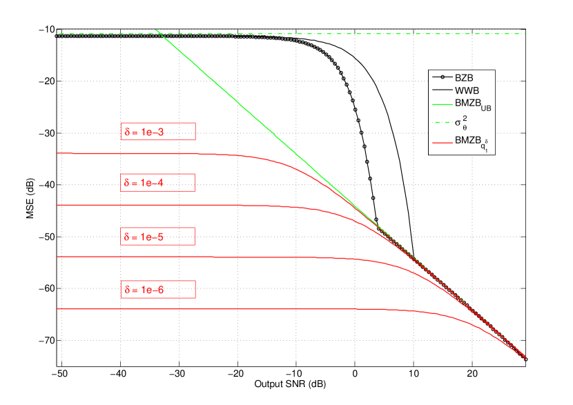
Figure 1: Single tone estimation: illustration of the relationship between $\mathrm{BZB}\left(\theta\right)$, $\mathrm{WWB}\left(\theta\right)$ (31a) and $\mathrm{BMZB}_{q_{1}^{\delta}}\left(\theta\right)$ (38a), $N=32$, SNR step is 0.5 dB.

Actually, this paradox can be explained by the fact that (32a):

$$\mathrm{BCRB}_{1_{\mathcal{S}_{\mathcal{X},\Theta}}}\left(\theta\right)=\underset{h\rightarrow 0}{\lim}\mathrm{BZB}^{h}\left(\theta\right)=\underset{h\rightarrow 0}{\lim}\left(\underset{s\rightarrow 1^{-}}{\lim}\mathrm{WWB}^{h,s}\left(\theta\right)\right)=\underset{h\rightarrow 0}{\lim}\frac{1}{\frac{2}{\left|h\right|}+\frac{4}{3}\pi^{2}\rho N\left(N-1\right)\left(2N-1\right)},$$ (43a)

is similar to:

$$\underset{\delta\rightarrow 0}{\lim}\mathrm{BMZB}_{q_{1}^{\delta}}\left(\theta\right)=\frac{\left(1-\delta\right)^{2}}{\frac{\pi^{2}}{4\delta}+\frac{4}{3}\pi^{2}\rho N\left(N-1\right)\left(2N-1\right)\left(1-\frac{5}{4}\delta\right)}=\underset{\delta\rightarrow 0}{\lim}\frac{1}{\frac{\pi^{2}}{4\delta}+\frac{4}{3}\pi^{2}\rho N\left(N-1\right)\left(2N-1\right)}$$ (43b)

provided that, for any $$\delta\ll 1 h\ll 1 \left|h\right|=8\delta/\pi^{2}$$ one chooses satisfying .

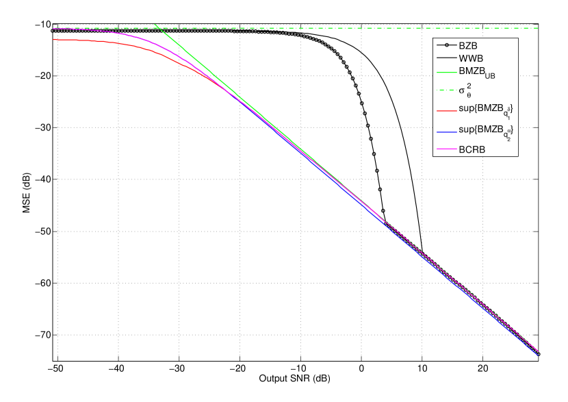
Figure 2: Single tone estimation: comparison of some BCRB (35a) obtained from two families of $\mathrm{BMZB}_{q}\left(\theta\right)$ (38a-38b), $N=32$, SNR step is 0.5 dB.

Therefore the limiting behavior of $\mathrm{BZB}^{h}\left(\theta\right)$ and $\mathrm{WWB}^{h,s}\left(\theta\right)$, where $h\rightarrow 0$, is the limiting behavior of $\mathrm{BMZB}_{q_{1}^{\delta}}\left(\theta\right)$, where $\delta\rightarrow 0$, which is exemplified in figure (1) as well, for $\delta\in\left\{10^{-3},10^{-4},10^{-5},10^{-6}\right\}$. As mentioned above, $\mathrm{BMZB}_{q_{1}^{\delta}}\left(\theta\right)$ always yields asymptotically $\mathrm{BMZB}_{UB}\left(\theta\right)$ but is also upper bounded by:

$$\mathrm{BMZB}_{q_{1}^{\delta}}\left(\theta\right)\leq\frac{4\delta}{\pi^{2}}$$ (44)

which tends to 0 when $\delta\rightarrow 0$. However, this adverse numerical behaviour can be easily circumvented by resorting to $\mathrm{BMZB}_{q_{1}^{\delta}}\left(\theta\right)$ and a tight BCRB in the asymptotic region can be obtained as $\underset{0<\delta\leq 0.5}{\sup}\left\{\mathrm{BMZB}_{q_{1}^{\delta}}\left(\theta\right)\right\}$ (35a), as shown in figure (2). It is also worth noting that some families of $\mathrm{BMZB}_{q}\left(\theta\right)$ does not allow to obtain a tight BCRB in the asymptotic region, as already mentioned in [3, pp 36-37], and again exemplified in the studied case in figure (2), if we consider $\underset{\alpha\geq\frac{3}{2}}{\sup}\left\{\mathrm{BMZB}_{q_{2}^{\alpha}}\left(\theta\right)\right\}$, which is however tight in the no-information region. Of course, one can combine the two families of $\mathrm{BMZB}$ as in (35a), in order to obtain a BCRB tight both in the asymptotic and the no-information region:

$$\mathrm{BCRB}\left(\theta\right)=\sup\left\{\underset{0<\delta\leq 0.5}{\sup}\left\{\mathrm{BMZB}_{q_{1}^{\delta}}\left(\theta\right)\right\},\underset{\alpha\geq\frac{3}{2}}{\sup}\left\{\mathrm{BMZB}_{q_{2}^{\alpha}}\left(\theta\right)\right\}\right\},$$ (45)

as also shown in figure (2).
Last, in figure (3) we display two different modified $\mathrm{WWB}_{q}\left(\theta\right)$ (39a), namely the $\mathrm{WWB}_{q_{1}^{0.5}}\left(\theta\right)$ and the $\mathrm{WWB}_{q_{2}^{2}}\left(\theta\right)$, and the associated modified $\mathrm{BZB}_{q_{1}^{0.5}}\left(\theta\right)$ and $\mathrm{BZB}_{q_{2}^{2}}\left(\theta\right),$ for a comparison with the $\mathrm{WWB}\left(\theta\right)$ (31a) and the associated $\mathrm{BZB}\left(\theta\right)$. Figure (3) highlights the following result: if the non zero limiting form of a large-error bound is tighter in the asymptotic region than the non zero limiting form of another large-error bound, this tightness relationship is still valid in the threshold region for the two large-error bounds.

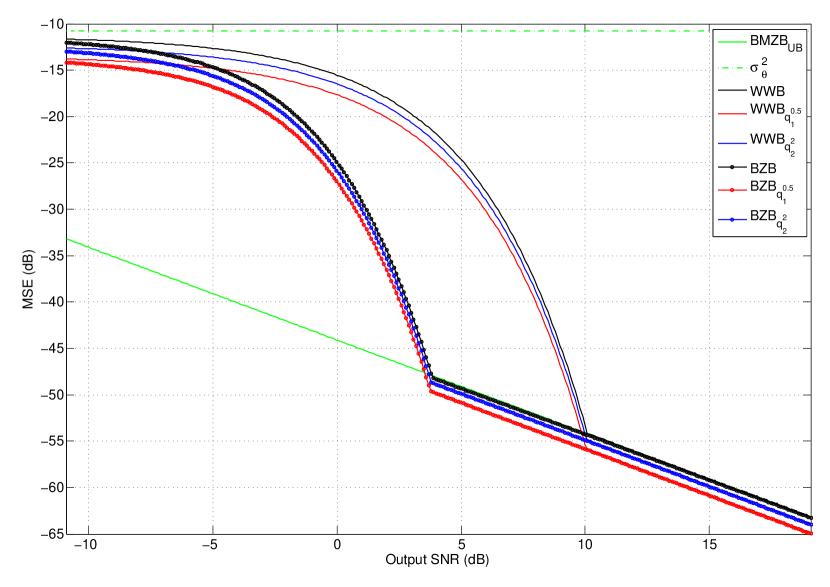
Figure 3: Single tone estimation: comparision of various modified BZBs and WWBs (39a), $N=32$, SNR step is 0.1 dB.

Although not displayed, we have checked this result in all the numerous comparisons we have done between representatives of $\mathrm{BMZB}_{q_{1}^{\delta}}\left(\theta\right)$ and $\mathrm{BMZB}_{q_{2}^{\alpha}}\left(\theta\right)$, within the same family or not. More precisely, we have noticed that for both the WWB and the BZB, the threshold value does not change (with a precision of 0.1 dB), but the relative bound tightness in the threshold region depends on the relative bound tightness in the asymptotic region. This observation allows to understand why the $\mathrm{WWB}\left(\theta\right)$ and the $\mathrm{BZB}\left(\theta\right)$ remain the tightest bounds in the threshold region. Indeed as:

$$\mathrm{WWB}\left(\theta\right)=\underset{\delta\rightarrow 0}{\lim}\left\{\mathrm{WWB}_{q_{1}^{\delta}}\left(\theta\right)\right\}\text{ and }\mathrm{BZB}\left(\theta\right)=\underset{\delta\rightarrow 0}{\lim}\left\{\mathrm{BZB}_{q_{1}^{\delta}}\left(\theta\right)\right\},$$ (46)

therefore, asymptotically, the limiting form of both the $\mathrm{WWB}\left(\theta\right)$ and the $\mathrm{BZB}\left(\theta\right)$ is $\mathrm{BMZB}_{q_{1}^{\delta}}\left(\theta\right)$, which asymptotically coincides with $\mathrm{BMZB}_{UB}\left(\theta\right)$, the tightest value of $\mathrm{BMZB}_{q}\left(\theta\right)$.

VI Conclusion

In the present paper, a fairly general class of ”large-error” BLBs of the WWF, essentially free from regularity conditions on the pdfs support and for which a limiting form yields a generalized BCRB, has been introduced. The proposed class of BLBs defines a wide range of Bayesian estimation problems for which a non trivial generalized BCRB exists, which is a key result from a practical viewpoint. In a large number of cases, this limiting form appears to be the BMZB. This theoretical result open new perspectives in the search of tight lower-bounds in the threshold region, new ones or some modified existing ones. Indeed, since the BMZB may provide a tighter bound than the historical BCRB in the asymptotic region, modified WWB and BZB which limiting form is the BMZB has been proposed. The analysis of the behavior of the proposed modified bounds in an application case has led us to postulate the following conjecture: if the non zero limiting form of a large-error bound is tighter in the asymptotic region than the non zero limiting form of another large-error bound, this tightness relationship is still valid in the threshold region for the two large-error bounds. Further study cases need to be addressed in order to quantify how general or specific is this conjecture.

VII Appendix

In this Appendix, Propositions 1 and its extension, Proposition 2, are derived.

VII-A Case of bounded intervals

First, let us address the case of closed intervals:

$$\forall\mathbf{x}\in\mathcal{S}_{\mathcal{X}},\quad\mathcal{S}_{\Theta|\mathbf{x}}=\left[a_{\mathbf{x}},b_{\mathbf{x}}\right]:-\infty<a_{\mathbf{x}}<b_{\mathbf{x}}<+\infty.$$ (47)

Step 1
First, one needs to asses:

$$\lim_{h\rightarrow 0}E_{\mathbf{x},\theta}\left[g\left(\theta\right)\frac{\psi_{q}^{h}\left(\mathbf{x},\theta\right)}{h}\right]=\lim_{h\rightarrow 0}E_{\mathbf{x},\theta}\left[\frac{g\left(\theta-h\right)-g\left(\theta\right)}{h}q\left(\mathbf{x},\theta\right)1_{\mathcal{S}_{\Theta|\mathbf{x}}}\left(\theta-h\right)\right]$$ (48)

According to (47), $\forall\mathbf{x}\in\mathcal{S}_{\mathcal{X}},\forall h>0$:

$$\begin{array}[]{c}E_{\theta|\mathbf{x}}\left[\frac{g\left(\theta-h\right)-g\left(\theta\right)}{h}q\left(\mathbf{x},\theta\right)1_{\mathcal{S}_{\Theta|\mathbf{x}}}\left(\theta-h\right)\right]=-\mathop{\displaystyle\int}\limits_{a_{\mathbf{x}}+h}^{b_{\mathbf{x}}}\left(\frac{g\left(\theta-h\right)-g\left(\theta\right)}{-h}\right)q\left(\mathbf{x},\theta\right)p\left(\theta|\mathbf{x}\right)d\theta\\ E_{\theta|\mathbf{x}}\left[\frac{g\left(\theta+h\right)-g\left(\theta\right)}{-h}q\left(\mathbf{x},\theta\right)1_{\mathcal{S}_{\Theta|\mathbf{x}}}\left(\theta+h\right)\right]=-\mathop{\displaystyle\int}\limits_{a_{\mathbf{x}}}^{b_{\mathbf{x}}-h}\left(\frac{g\left(\theta+h\right)-g\left(\theta\right)}{h}\right)q\left(\mathbf{x},\theta\right)p\left(\theta|\mathbf{x}\right)d\theta\end{array}\quad$$ (49a)

Assuming that $$g\left(\theta\right) \mathcal{C}^{1} \mathcal{S}_{\Theta|\mathbf{x}}$$ is of class over , by invoking the mean value theorem [20], one obtains

$$\begin{array}[]{c}\exists\gamma^{+}\left(h\right)\in\left[0,h\right]:\frac{g\left(\theta+h\right)-g\left(\theta\right)}{h}=\frac{dg\left(\theta+\gamma^{+}\left(h\right)\right)}{d\theta}\\ \exists\gamma^{-}\left(h\right)\in\left[0,h\right]:\frac{g\left(\theta\right)-g\left(\theta-h\right)}{h}=\frac{dg\left(\theta-\gamma^{-}\left(h\right)\right)}{d\theta}\end{array}$$ (49b)

Thus, we deduce that, $$\forall\mathbf{x}\in\mathcal{S}_{\mathcal{X}}:$$

$$\begin{array}[]{l}\lim\limits_{h\rightarrow 0^{+}}E_{\theta|\mathbf{x}}\left[\frac{g\left(\theta-h\right)-g\left(\theta\right)}{h}q\left(\mathbf{x},\theta\right)1_{\mathcal{S}_{\Theta|\mathbf{x}}}\left(\theta-h\right)\right]=-\lim\limits_{h\rightarrow 0^{+}}\mathop{\displaystyle\int}\limits_{a_{\mathbf{x}}+h}^{b_{\mathbf{x}}}\frac{dg\left(\theta\right)}{d\theta}q\left(\mathbf{x},\theta\right)p\left(\theta|\mathbf{x}\right)d\theta\\ \qquad\qquad\qquad\qquad\qquad\qquad\qquad\qquad~{}+\lim\limits_{h\rightarrow 0^{+}}\mathop{\displaystyle\int}\limits_{a_{\mathbf{x}}+h}^{b_{\mathbf{x}}}\left(\frac{dg\left(\theta\right)}{d\theta}-\frac{dg\left(\theta-\gamma^{-}\left(h\right)\right)}{d\theta}\right)q\left(\mathbf{x},\theta\right)p\left(\theta|\mathbf{x}\right)d\theta\end{array}$$ (49e)

$$\begin{array}[]{l}\lim\limits_{h\rightarrow 0^{+}}E_{\theta|\mathbf{x}}\left[\frac{g\left(\theta+h\right)-g\left(\theta\right)}{-h}q\left(\mathbf{x},\theta\right)1_{\mathcal{S}_{\Theta|\mathbf{x}}}\left(\theta+h\right)\right]=-\lim\limits_{h\rightarrow 0^{+}}\mathop{\displaystyle\int}\limits_{a_{\mathbf{x}}}^{b_{\mathbf{x}}-h}\frac{dg\left(\theta\right)}{d\theta}q\left(\mathbf{x},\theta\right)p\left(\theta|\mathbf{x}\right)d\theta\\ \qquad\qquad\qquad\qquad\qquad\qquad\qquad\qquad~{}+\lim\limits_{h\rightarrow 0^{+}}\mathop{\displaystyle\int}\limits_{a_{\mathbf{x}}}^{b_{\mathbf{x}}-h}\left(\frac{dg\left(\theta\right)}{d\theta}-\frac{dg\left(\theta+\gamma^{+}\left(h\right)\right)}{d\theta}\right)q\left(\mathbf{x},\theta\right)p\left(\theta|\mathbf{x}\right)d\theta\end{array}$$ (49h)

According to Heine theorem [20]:

$$\forall\varepsilon>0,\exists h>0~{}|~{}\forall\left(\theta,\theta^{\prime}\right)\in\mathcal{S}_{\theta|\mathbf{x}},\left|\theta-\theta^{\prime}\right|<h~{}\Rightarrow~{}\left|\frac{dg\left(\theta\right)}{d\theta}-\frac{dg\left(\theta^{\prime}\right)}{d\theta}\right|<\varepsilon,$$ (50a)

one can state that

$$\forall\varepsilon>0,\exists h>0~{}|~{}\left\{\begin{array}[]{c}\forall\gamma^{+}\left(h\right)<h~{}\Rightarrow~{}\left|\frac{dg\left(\theta\right)}{d\theta}-\frac{dg\left(\theta+\gamma^{+}\left(h\right)\right)}{d\theta}\right|<\varepsilon\\ \forall\gamma^{-}\left(h\right)<h~{}\Rightarrow~{}\left|\frac{dg\left(\theta\right)}{d\theta}-\frac{dg\left(\theta-\gamma^{-}\left(h\right)\right)}{d\theta}\right|<\varepsilon\end{array}\right..$$ (50b)

Consequently,$$\forall\mathbf{x}\in\mathcal{S}_{\mathcal{X}} \forall\varepsilon>0,\exists h>0$$, such that:

$$\left|\mathop{\displaystyle\int}\limits_{a_{\mathbf{x}}+h}^{b_{\mathbf{x}}}\left(\begin{array}[]{l}\frac{dg\left(\theta\right)}{d\theta}-\\ \frac{dg\left(\theta-\gamma^{-}\left(h\right)\right)}{d\theta}\end{array}\right)q\left(\mathbf{x},\theta\right)p\left(\theta|\mathbf{x}\right)d\theta\right| \leq \mathop{\displaystyle\int}\limits_{a_{\mathbf{x}}+h}^{b_{\mathbf{x}}}\left|\frac{dg\left(\theta\right)}{d\theta}-\frac{dg\left(\theta-\gamma^{-}\left(h\right)\right)}{d\theta}\right|\left|q\left(\mathbf{x},\theta\right)\right|p\left(\theta|\mathbf{x}\right)d\theta\qquad\quad$$ (50e)

$$\leq \mathop{\displaystyle\int}\limits_{a_{\mathbf{x}}}^{b_{\mathbf{x}}}\left|\frac{dg\left(\theta\right)}{d\theta}-\frac{dg\left(\theta-\gamma^{-}\left(h\right)\right)}{d\theta}\right|\left|q\left(\mathbf{x},\theta\right)\right|p\left(\theta|\mathbf{x}\right)d\theta$$ (50f)

$$< \varepsilon E_{\theta|\mathbf{x}}\left[\left|q\left(\mathbf{x},\theta\right)\right|\right]$$ (50g)

leading to:

$$\forall\mathbf{x}\in\mathcal{S}_{\mathcal{X}}:\lim_{h\rightarrow 0}E_{\theta|\mathbf{x}}\left[g\left(\theta\right)\frac{\psi_{q}^{h}\left(\mathbf{x},\theta\right)}{h}\right]=-E_{\theta|\mathbf{x}}\left[\frac{\partial g\left(\theta\right)}{\partial\theta}q\left(\mathbf{x},\theta\right)\right],$$ (51a)

and:

$$\lim_{h\rightarrow 0}E_{\mathbf{x},\theta}\left[g\left(\theta\right)\frac{\psi_{q}^{h}\left(\mathbf{x},\theta\right)}{h}\right]=-E_{\mathbf{x},\theta}\left[\frac{\partial g\left(\theta\right)}{\partial\theta}q\left(\mathbf{x},\theta\right)\right].$$ (51b)

Step 2
Second, one needs to asses:

$$\lim_{h\rightarrow 0}E_{\mathbf{x},\theta}\left[\left(\frac{\psi_{q}^{h}\left(\mathbf{x},\theta\right)}{h}\right)^{2}\right].$$ (52)

According to (47), $\forall\mathbf{x}\in\mathcal{S}_{\mathcal{X}},\forall h>0$:

$$E_{\theta|\mathbf{x}}\left[\frac{\psi_{q}^{h}\left(\mathbf{x},\theta\right)^{2}}{h^{2}}\right] = \frac{1}{h^{2}}\mathop{\displaystyle\int}\limits_{a_{\mathbf{x}}}^{b_{\mathbf{x}}}\left(\begin{array}[]{l}q\left(\mathbf{x},\theta+h\right)p\left(\theta+h|\mathbf{x}\right)1_{\mathcal{S}_{\theta{|\mathbf{x}}}}\left(\theta+h\right)\\ -q\left(\mathbf{x},\theta\right)p\left(\theta|\mathbf{x}\right)1_{\mathcal{S}_{\Theta|\mathbf{x}}}\left(\theta-h\right)\end{array}\right)^{2}\frac{d\theta}{p\left(\theta|\mathbf{x}\right)}$$ (53c)

$$E_{\theta|\mathbf{x}}\left[\frac{\psi_{q}^{h}\left(\mathbf{x},\theta\right)^{2}}{h^{2}}\right] = \begin{array}[]{l}\mathop{\displaystyle\int}\limits_{a_{\mathbf{x}}}^{b_{\mathbf{x}}-h}\frac{\left(q\left(\mathbf{x},\theta+h\right)p\left(\theta+h|\mathbf{x}\right)-q\left(\mathbf{x},\theta\right)p\left(\theta|\mathbf{x}\right)\right)^{2}}{h^{2}}\frac{d\theta}{p\left(\theta|\mathbf{x}\right)}\\ +\frac{2}{h}\mathop{\displaystyle\int}\limits_{a_{\mathbf{x}}}^{a_{\mathbf{x}}+h}\frac{q\left(\mathbf{x},\theta+h\right)p\left(\theta+h|\mathbf{x}\right)-q\left(\mathbf{x},\theta\right)p\left(\theta|\mathbf{x}\right)}{h}q\left(\mathbf{x},\theta\right)d\theta\\ +\frac{1}{h^{2}}\left(\mathop{\displaystyle\int}\limits_{a_{\mathbf{x}}}^{a_{\mathbf{x}}+h}q\left(\mathbf{x},\theta\right)^{2}p\left(\theta|\mathbf{x}\right)d\theta+\mathop{\displaystyle\int}\limits_{b_{\mathbf{x}}-h}^{b_{\mathbf{x}}}q\left(\mathbf{x},\theta\right)^{2}p\left(\theta|\mathbf{x}\right)d\theta\right)\end{array}$$ (53g)

and

$$E_{\theta|\mathbf{x}}\left[\frac{\psi_{q}^{-h}\left(\mathbf{x},\theta\right)^{2}}{\left(-h\right)^{2}}\right] = \frac{1}{h^{2}}\mathop{\displaystyle\int}\limits_{a_{\mathbf{x}}}^{b_{\mathbf{x}}}\left(\begin{array}[]{l}q\left(\mathbf{x},\theta-h\right)p\left(\theta-h|\mathbf{x}\right)1_{\mathcal{S}_{\theta|\mathbf{x}}}\left(\theta-h\right)\\ -q\left(\mathbf{x},\theta\right)p\left(\theta|\mathbf{x}\right)1_{\mathcal{S}_{\theta|\mathbf{x}}}\left(\theta+h\right)\end{array}\right)^{2}\frac{d\theta}{p\left(\theta|\mathbf{x}\right)}$$ (53j)

$$E_{\theta|\mathbf{x}}\left[\frac{\psi_{q}^{-h}\left(\mathbf{x},\theta\right)^{2}}{\left(-h\right)^{2}}\right] = \begin{array}[]{l}\mathop{\displaystyle\int}\limits_{a_{\mathbf{x}}+h}^{b_{\mathbf{x}}}\frac{\left(q\left(\mathbf{x},\theta+h\right)p\left(\theta+h|\mathbf{x}\right)-q\left(\mathbf{x},\theta\right)p\left(\theta|\mathbf{x}\right)\right)^{2}}{\left(-h\right)^{2}}\frac{d\theta}{p\left(\theta|\mathbf{x}\right)}\\ -\frac{2}{h}\mathop{\displaystyle\int}\limits_{b_{\mathbf{x}}-h}^{b_{\mathbf{x}}}\frac{q\left(\mathbf{x},\theta-h\right)p\left(\theta-h|\mathbf{x}\right)-q\left(\mathbf{x},\theta\right)p\left(\theta|\mathbf{x}\right)}{-h}q\left(\mathbf{x},\theta\right)d\theta\\ +\frac{1}{h^{2}}\left(\mathop{\displaystyle\int}\limits_{a_{\mathbf{x}}}^{a_{\mathbf{x}}+h}q\left(\mathbf{x},\theta\right)^{2}p\left(\theta|\mathbf{x}\right)d\theta+\mathop{\displaystyle\int}\limits_{b_{\mathbf{x}}-h}^{b_{\mathbf{x}}}q\left(\mathbf{x},\theta\right)^{2}p\left(\theta|\mathbf{x}\right)d\theta\right)\end{array}$$ (53n)

Assuming that $t\left(\mathbf{x},\theta\right)=q\left(\mathbf{x},\theta\right)p\left(\theta|\mathbf{x}\right)$ is of class $\mathcal{C}^{1}$ w.r.t. $\theta$ over $\mathcal{S}_{\Theta|\mathbf{x}}$, thus $\left(\frac{\partial t\left(\mathbf{x},\theta\right)}{\partial\theta}\right)^{2}$ is continuous over $\mathcal{S}_{\Theta|\mathbf{x}}$. Then, using the same rationale as in step 1 based on the mean value theorem and the Heine theorem, one can easily prove that, $\forall\mathbf{x}\in\mathcal{S}_{\mathcal{X}}$:

$$\lim\limits_{h\rightarrow 0^{+}}E_{\theta|\mathbf{x}}\left[\left(\frac{\psi_{q}^{h}\left(\mathbf{x},\theta\right)}{h}\right)^{2}\right]=\begin{array}[]{l}E_{\theta|\mathbf{x}}\left[\left(\frac{1}{p\left(\theta|\mathbf{x}\right)}\frac{\partial t\left(\mathbf{x},\theta\right)}{\partial\theta}\right)^{2}\right]+2q\left(\mathbf{x},a_{\mathbf{x}}\right)\left.\frac{\partial t\left(\mathbf{x},\theta\right)}{\partial\theta}\right|_{\theta=a_{\mathbf{x}}}\\ +\frac{1}{h^{2}}\left(\mathop{\displaystyle\int}\limits_{a_{\mathbf{x}}}^{a_{\mathbf{x}}+h}u\left(\mathbf{x},\theta\right)d\theta+\mathop{\displaystyle\int}\limits_{b_{\mathbf{x}}-h}^{b_{\mathbf{x}}}u\left(\mathbf{x},\theta\right)d\theta\right)\end{array}$$ (53o)

and

$$\lim\limits_{h\rightarrow 0^{+}}E_{\theta|\mathbf{x}}\left[\left(\frac{\psi_{q}^{-h}\left(\mathbf{x},\theta\right)}{-h}\right)^{2}\right]=\begin{array}[]{l}E_{\theta|\mathbf{x}}\left[\left(\frac{1}{p\left(\theta|\mathbf{x}\right)}\frac{\partial t\left(\mathbf{x},\theta\right)}{\partial\theta}\right)^{2}\right]-2q\left(\mathbf{x},b_{\mathbf{x}}\right)\left.\frac{\partial t\left(\mathbf{x},\theta\right)}{\partial\theta}\right|_{\theta=b_{\mathbf{x}}}\\ +\frac{1}{h^{2}}\left(\mathop{\displaystyle\int}\limits_{a_{\mathbf{x}}}^{a_{\mathbf{x}}+h}u\left(\mathbf{x},\theta\right)d\theta+\mathop{\displaystyle\int}\limits_{b_{\mathbf{x}}-h}^{b_{\mathbf{x}}}u\left(\mathbf{x},\theta\right)d\theta\right)\end{array}$$ (53p)

where $u\left(\mathbf{x},\theta\right)=t\left(\mathbf{x},\theta\right)q\left(\mathbf{x},\theta\right)=q\left(\mathbf{x},\theta\right)^{2}p\left(\theta|\mathbf{x}\right)$. Assuming that $u\left(\mathbf{x},\theta\right)$ is of class $\mathcal{C}^{2}$ w.r.t. $\theta$ at the vicinity of endpoints $a_{\mathbf{x}}$ and $b_{\mathbf{x}}$, one can prove that (see appendix VII-D):

$$\lim_{h\rightarrow 0^{+}}\frac{1}{h^{2}}\left(\mathop{\displaystyle\int}\limits_{a_{\mathbf{x}}}^{a_{\mathbf{x}}+h}u\left(\mathbf{x},\theta\right)d\theta+\mathop{\displaystyle\int}\limits_{b_{\mathbf{x}}-h}^{b_{\mathbf{x}}}u\left(\mathbf{x},\theta\right)d\theta\right)=\frac{u\left(\mathbf{x},b_{\mathbf{x}}\right)+u\left(\mathbf{x},a_{\mathbf{x}}\right)}{h}\\ +\frac{1}{2}\left(\left.\frac{\partial u\left(\mathbf{x},{\theta}\right)}{\partial\theta}\right|_{\theta=a_{\mathbf{x}}}-\left.\frac{\partial u\left(\mathbf{x},{\theta}\right)}{\partial\theta}\right|_{\theta=b_{\mathbf{x}}}\right)$$ (54)

Therefore, in order to obtain a non trivial $\mathrm{BCRB}_{q}$ from (53o-53p), the following necessary and sufficient conditions must hold:

$$u\left(\mathbf{x},b_{\mathbf{x}}\right)+u\left(\mathbf{x},a_{\mathbf{x}}\right)=q\left(\mathbf{x},a_{\mathbf{x}}\right)^{2}p\left(a_{\mathbf{x}}|\mathbf{x}\right)+q\left(\mathbf{x},b_{\mathbf{x}}\right)^{2}p\left(b_{\mathbf{x}}|\mathbf{x}\right)=0,$$ (55a)

that is:

$$q\left(\mathbf{x},a_{\mathbf{x}}\right)p\left(a_{\mathbf{x}}|\mathbf{x}\right)=0\text{ and }q\left(\mathbf{x},b_{\mathbf{x}}\right)p\left(b_{\mathbf{x}}|\mathbf{x}\right)=0.$$ (55b)

Plugging (55b) into the following identities

$$\frac{\partial u\left(\mathbf{x},\theta\right)}{\partial\theta} = 2\frac{\partial q\left(\mathbf{x},\theta\right)}{\partial\theta}q\left(\mathbf{x},\theta\right)p\left(\theta|\mathbf{x}\right)+q\left(\mathbf{x},\theta\right)^{2}\frac{\partial p\left(\theta|\mathbf{x}\right)}{\partial\theta},$$ (55c)

$$\frac{\partial t\left(\mathbf{x},\theta\right)}{\partial\theta}q\left(\mathbf{x},\theta\right) = \frac{\partial q\left(\mathbf{x},\theta\right)}{\partial\theta}q\left(\mathbf{x},\theta\right)p\left(\theta|\mathbf{x}\right)+q\left(\mathbf{x},\theta\right)^{2}\frac{\partial p\left(\theta|\mathbf{x}\right)}{\partial\theta^{2}},$$ (55d)

one obtains

$$\left.\frac{\partial t\left(\mathbf{x},\theta\right)}{\partial\theta}\right|_{\theta=a_{\mathbf{x}}}q\left(\mathbf{x},a_{\mathbf{x}}\right) = q\left(\mathbf{x},a_{\mathbf{x}}\right)^{2}\left.\frac{\partial p\left({\theta}|\mathbf{x}\right)}{\partial\theta}\right|_{\theta=a_{\mathbf{x}}}=\left.\frac{\partial u\left(\mathbf{x},{\theta}\right)}{\partial\theta}\right|_{\theta=a_{\mathbf{x}}},$$ (55e)

$$\left.\frac{\partial t\left(\mathbf{x},\theta\right)}{\partial\theta}\right|_{\theta=b_{\mathbf{x}}}q\left(\mathbf{x},a_{\mathbf{x}}\right) = q\left(\mathbf{x},b_{\mathbf{x}}\right)^{2}\left.\frac{\partial p\left({\theta}|\mathbf{x}\right)}{\partial\theta}\right|_{\theta=b_{\mathbf{x}}}=\left.\frac{\partial u\left(\mathbf{x},\theta\right)}{\partial\theta}\right|_{\theta=b_{\mathbf{x}}},$$ (55f)

leading to, $$\forall\mathbf{x}\in\mathcal{S}_{\mathcal{X}}:$$

$$\lim\limits_{h\rightarrow 0^{+}}E_{\theta|\mathbf{x}}\left[\left(\frac{\psi_{q}^{h}\left(\mathbf{x},\theta\right)}{h}\right)^{2}\right] = \begin{array}[]{l}E_{\theta|\mathbf{x}}\left[\left(\frac{1}{p\left(\theta|\mathbf{x}\right)}\frac{\partial t\left(\mathbf{x},\theta\right)}{\partial\theta}\right)^{2}\right]\\ +\frac{5}{2}q\left(\mathbf{x},a_{\mathbf{x}}\right)^{2}\left.\frac{\partial p\left({\theta}|\mathbf{x}\right)}{\partial\theta}\right|_{\theta=a_{\mathbf{x}}}-\frac{1}{2}q\left(\mathbf{x},b_{\mathbf{x}}\right)^{2}\left.\frac{\partial p\left(\theta|\mathbf{x}\right)}{\partial\theta}\right|_{\theta=b_{\mathbf{x}}}\end{array}$$ (56c)

$$\lim\limits_{h\rightarrow 0^{+}}E_{\theta|\mathbf{x}}\left[\left(\frac{\psi_{q}^{-h}\left(\mathbf{x},\theta\right)}{-h}\right)^{2}\right] = \begin{array}[]{l}E_{\theta|\mathbf{x}}\left[\left(\frac{1}{p\left(\theta|\mathbf{x}\right)}\frac{\partial t\left(\mathbf{x},\theta\right)}{\partial\theta}\right)^{2}\right]\\ -\frac{5}{2}q\left(\mathbf{x},b_{\mathbf{x}}\right)^{2}\left.\frac{\partial p\left({\theta}|\mathbf{x}\right)}{\partial\theta}\right|_{\theta=b_{\mathbf{x}}}+\frac{1}{2}q\left(\mathbf{x},a_{\mathbf{x}}\right)^{2}\left.\frac{\partial p\left({\theta}|\mathbf{x}\right)}{\partial\theta}\right|_{\theta=a_{\mathbf{x}}}\end{array}$$ (56f)

Furthermore, the endpoints condition $$u\left(\mathbf{x},a_{\mathbf{x}}\right)=0 u\left(\mathbf{x},b_{\mathbf{x}}\right)=0 u\left(\mathbf{x},\theta\right) a_{\mathbf{x}} b_{\mathbf{x}}$$ and implies that the function is increasing at the vicinity of and decreasing at the vicinity of . Thus:

$$\frac{5}{2}q\left(\mathbf{x},a_{\mathbf{x}}\right)^{2}\left.\frac{\partial p\left({\theta}|\mathbf{x}\right)}{\partial\theta}\right|_{\theta=a_{\mathbf{x}}}-\frac{1}{2}q\left(\mathbf{x},b_{\mathbf{x}}\right)^{2}\left.\frac{\partial p\left({\theta}|\mathbf{x}\right)}{\partial\theta}\right|_{\theta=b_{\mathbf{x}}}\geq 0$$ (57a)

and

$$-\frac{5}{2}q\left(\mathbf{x},b_{\mathbf{x}}\right)^{2}\left.\frac{\partial p\left({\theta}|\mathbf{x}\right)}{\partial\theta}\right|_{\theta=b_{\mathbf{x}}}+\frac{1}{2}q\left(\mathbf{x},a_{\mathbf{x}}\right)^{2}\left.\frac{\partial p\left({\theta}|\mathbf{x}\right)}{\partial\theta}\right|_{\theta=a_{\mathbf{x}}}\geq 0$$ (57b)

Consequently:

$$\lim\limits_{h\rightarrow 0}E_{\theta|\mathbf{x}}\left[\left(\frac{\psi_{q}^{h}\left(\mathbf{x},\theta\right)}{h}\right)^{2}\right]\geq E_{\theta|\mathbf{x}}\left[\left(\frac{1}{p\left(\theta|\mathbf{x}\right)}\frac{\partial t\left(\mathbf{x},\theta\right)}{\partial\theta}\right)^{2}\right]$$ (58a)

in which, the equality holds for $$q\left(\mathbf{x},a_{\mathbf{x}}\right)=q\left(\mathbf{x},b_{\mathbf{x}}\right)=0 v\left(\mathbf{x},\theta\right)=q\left(\mathbf{x},\theta\right)^{2}\frac{\partial p\left(\theta|\mathbf{x}\right)}{\partial\theta} \mathbf{x}$$. Last, let ; by taking the expectation with respect to of (56c-56f), one gets the following inequality:

$$\lim\limits_{h\rightarrow 0}E_{\mathbf{x},\theta}\left[\left(\frac{\psi_{q}^{h}\left(\mathbf{x},\theta\right)}{h}\right)^{2}\right]\leq E_{\mathbf{x},\theta}\left[\left(\frac{\frac{\partial t\left(\mathbf{x},\theta\right)}{\partial\theta}}{p\left(\theta|\mathbf{x}\right)}\right)^{2}\right]+\min\left\{\begin{array}[]{l}E_{\mathbf{x}}\left[\frac{5}{2}v\left(\mathbf{x},a_{\mathbf{x}}\right)-\frac{1}{2}v\left(\mathbf{x},b_{\mathbf{x}}\right)\right],\\ E_{\mathbf{x}}\left[\frac{1}{2}v\left(\mathbf{x},a_{\mathbf{x}}\right)-\frac{5}{2}v\left(\mathbf{x},b_{\mathbf{x}}\right)\right]\end{array}\right\},$$ (58b)

which, combined with (51b) lead to (15b).
It is straightforward to extend the above rationale to the general case of bounded intervals $$\mathcal{S}_{\Theta|\mathbf{x}}=\left[a_{\mathbf{x}},b_{\mathbf{x}}\right[ \mathcal{S}_{\Theta|\mathbf{x}}=\left]a_{\mathbf{x}},b_{\mathbf{x}}\right] \mathcal{S}_{\Theta|\mathbf{x}}=\left]a_{\mathbf{x}},b_{\mathbf{x}}\right[ -\infty<a_{\mathbf{x}}<b_{\mathbf{x}}<+\infty q\left(\mathbf{x},\theta\right) \frac{\partial t\left(\mathbf{x},\theta\right)}{\partial\theta} u\left(\mathbf{x},{\theta}\right) \frac{\partial u\left(\mathbf{x},\theta\right)}{\partial\theta} \frac{\partial^{2}u\left(\mathbf{x},\theta\right)}{\partial^{2}\theta} a_{\mathbf{x}} b_{\mathbf{x}} g\left(\theta\right) q\left(\mathbf{x},\theta\right)p\left(\theta|\mathbf{x}\right) \mathcal{C}^{1} \theta \mathcal{S}_{\Theta|\mathbf{x}}$$, , , , provided that : , , , and are bounded functions at the vicinity of endpoints and .
Moreover, (58b) is uniquely integral calculus based, thus, due to the fact that the result does not change by a finite number of discontinuities, we conclude that the above conditions can be relaxed to : and are piecewise function w.r.t. over .

VII-B Case of unbounded intervals

In the case of unbounded intervals, one has $a_{\mathbf{x}}=-\infty$ and/or $b_{\mathbf{x}}=+\infty$. Then, let us define a sequence of intervals given by

$$\mathcal{S}_{\Theta|\mathbf{x}}^{l}=\left]a_{\mathbf{x}}^{l},b_{\mathbf{x}}^{l}\right[,-\infty<a_{\mathbf{x}}^{l}<b_{\mathbf{x}}^{l}<\infty\text{ subject to }\mathcal{S}_{\Theta|\mathbf{x}}^{l}\subset\mathcal{S}_{\Theta|\mathbf{x}}\text{ and }\lim\limits_{l\rightarrow\infty}\mathcal{S}_{\Theta|\mathbf{x}}^{l}=\mathcal{S}_{\Theta|\mathbf{x}}$$

In the same way, we define $\mathcal{S}_{\mathcal{X},\Theta}^{l}=\left\{\left(\mathbf{x},\theta\right)~{}|~{}\mathbf{x}\in\mathcal{S}_{\mathcal{X}}\text{ and }\theta\in\mathcal{S}_{\Theta|\mathbf{x}}^{l}\right\}$ and denote:

$$p^{l}\left(\mathbf{x},\theta\right)=\frac{p\left(\mathbf{x},\theta\right)}{\mathop{\displaystyle\iint}\limits_{\mathcal{S}_{\mathcal{X},\Theta}^{l}}p\left(\mathbf{x},\theta\right)d\mathbf{x}d\theta},\text{\quad}p^{l}\left(\theta|\mathbf{x}\right)=\frac{p\left(\theta|\mathbf{x}\right)}{\mathop{\displaystyle\int}\limits_{\mathcal{S}_{\Theta|\mathbf{x}}^{l}}p\left(\theta|\mathbf{x}\right)d\theta},$$ (59a)

which defines:

$$E_{\mathbf{x},\theta}^{l}\left[q\left(\mathbf{x},\theta\right)\right]=\mathop{\displaystyle\iint}\limits_{\mathcal{S}_{\mathcal{X},\Theta}^{l}}q\left(\mathbf{x},\theta\right)p^{l}\left(\mathbf{x},\theta\right)d\mathbf{x}d\theta,\text{\quad}E_{\theta|\mathbf{x}}^{l}\left[q\left(\mathbf{x},\theta\right)\right]=\mathop{\displaystyle\int}\limits_{\mathcal{S}_{\Theta|\mathbf{x}}^{l}}q\left(\mathbf{x},\theta\right)p^{l}\left(\theta|\mathbf{x}\right)d\theta$$ (59b)

Then, the analysis and results given in the previous Section VII-A can be applied to the restricted intervals $$\mathcal{S}_{\mathcal{X},\Theta}^{l},\mathcal{S}_{\Theta|\mathbf{x}}^{l} p^{l}\left(\mathbf{x},\theta\right),p^{l}\left(\theta|\mathbf{x}\right)$$ and their associated pdfs , respectively. By definition:

$$\mathop{\displaystyle\iint}\limits_{\mathcal{S}_{\mathcal{X},\Theta}}\left(E_{\theta|\mathbf{x}}\left[g\left(\theta\right)\right]-g\left(\theta\right)\right)^{2}p^{l}(\mathbf{x},\theta)d\theta d\mathbf{x}\geq\mathop{\displaystyle\iint}\limits_{\mathcal{S}_{\mathcal{X},\Theta}^{l}}\left(E_{\theta|\mathbf{x}}\left[g\left(\theta\right)\right]-g\left(\theta\right)\right)^{2}p^{l}(\mathbf{x},\theta)d\theta d\mathbf{x},$$ (60a)

that is:

$$\frac{E_{\mathbf{x},\theta}\left[\left(E_{\theta|\mathbf{x}}\left[g\left(\theta\right)\right]-g\left(\theta\right)\right)^{2}\right]}{\mathop{\displaystyle\iint}\limits_{\mathcal{S}^{l}}p\left(\mathbf{x},\theta\right)d\mathbf{x}d\theta}\geq E_{\mathbf{x},\theta}^{l}\left[\left(E_{\theta|\mathbf{x}}\left[g\left(\theta\right)\right]-g\left(\theta\right)\right)^{2}\right].$$ (60b)

Moreover, as:

$$E_{\mathbf{x},\theta}^{l}\left[\left(E_{\theta|\mathbf{x}}\left[g\left(\theta\right)\right]-g\left(\theta\right)\right)^{2}\right]\geq E_{\mathbf{x},\theta}^{l}\left[\left(E_{\theta|\mathbf{x}}^{l}\left[g\left(\theta\right)\right]-g\left(\theta\right)\right)^{2}\right],$$ (60c)

therefore:

$$\frac{E_{\mathbf{x},\theta}\left[\left(E_{\theta|\mathbf{x}}\left[g\left(\theta\right)\right]-g\left(\theta\right)\right)^{2}\right]}{\mathop{\displaystyle\iint}\limits_{\mathcal{S}_{\mathcal{X},\Theta}^{l}}p\left(\mathbf{x},\theta\right)d\mathbf{x}d\theta}\geq E_{\mathbf{x},\theta}^{l}\left[\left(E_{\theta|\mathbf{x}}^{l}\left[g\left(\theta\right)\right]-g\left(\theta\right)\right)^{2}\right].$$ (60d)

Finally, since $$\lim\limits_{l\rightarrow\infty}\mathcal{S}_{\Theta|\mathbf{x}}^{l}=\mathcal{S}_{\Theta|\mathbf{x}}$$, one has:

$$E_{\mathbf{x},\theta}\left[\left(E_{\theta|\mathbf{x}}\left[g\left(\theta\right)\right]-g\left(\theta\right)\right)^{2}\right]\geq\lim\limits_{l\rightarrow\infty}E_{\mathbf{x},\theta}^{l}\left[\left(E_{\theta|\mathbf{x}}^{l}\left[g\left(\theta\right)\right]-g\left(\theta\right)\right)^{2}\right],$$ (60e)

which allows to state Proposition 1 as the limiting form of the bounded intervals case.

VII-C Case of a countable union of disjoint intervals of $\mathbb{R}$

First we consider the case where $\mathcal{S}_{\Theta|\mathbf{x}}$ results from a finite union of disjoint bounded intervals $\mathcal{I}_{\Theta|\mathbf{x}}^{k}\varsubsetneq\mathbb{R}$:

$$\forall\mathbf{x}\in\mathcal{S}_{\mathcal{X}},\quad\mathcal{S}_{\Theta|\mathbf{x}}=\mathop{\textstyle\bigcup}\limits_{1\leq k\leq K_{\mathbf{x}}}\mathcal{I}_{\Theta|\mathbf{x}}^{k},\text{ such that\ }K_{\mathbf{x}}\in\mathbb{N}\text{ and }\mathcal{I}_{\Theta|\mathbf{x}}^{k}\cap\mathcal{I}_{\Theta|\mathbf{x}}^{l}=\varnothing\text{ if }k\neq l.$$

Let us denote the endpoints of $\mathcal{I}_{\Theta|\mathbf{x}}^{k}$ by $a_{\mathbf{x}}^{k}$ and $b_{\mathbf{x}}^{k}$, $a_{\mathbf{x}}^{k}<a_{\mathbf{x}}^{k}$. Then

$$\left\{\begin{array}[]{l}E_{\theta|\mathbf{x}}\left[g\left(\theta\right)\frac{\psi_{q}^{h}\left(\mathbf{x},\theta\right)}{h}\right]=-\mathop{\textstyle\sum}\limits_{k=1}^{K_{\mathbf{x}}}\mathop{\displaystyle\int}\limits_{a_{\mathbf{x}}^{k}+h}^{b_{\mathbf{x}}^{k}}\left(\frac{g\left(\theta-h\right)-g\left(\theta\right)}{-h}\right)q\left(\mathbf{x},\theta\right)p\left(\theta|\mathbf{x}\right)d\theta,\\ E_{\theta|\mathbf{x}}\left[g\left(\theta\right)\frac{\psi_{q}^{h}\left(\mathbf{x},\theta\right)}{h}\right]=-\mathop{\textstyle\sum}\limits_{k=1}^{K_{\mathbf{x}}}\mathop{\displaystyle\int}\limits_{a_{\mathbf{x}}^{k}}^{b_{\mathbf{x}}^{k}-h}\left(\frac{g\left(\theta+h\right)-g\left(\theta\right)}{h}\right)q\left(\mathbf{x},\theta\right)p\left(\theta|\mathbf{x}\right)d\theta,\\ E_{\theta|\mathbf{x}}\left[\frac{\psi_{q}^{h}\left(\mathbf{x},\theta\right)^{2}}{h^{2}}\right]=\frac{1}{h^{2}}\mathop{\textstyle\sum}\limits_{k=1}^{K_{\mathbf{x}}}\mathop{\displaystyle\int}\limits_{a_{\mathbf{x}}^{k}+h}^{b_{\mathbf{x}}^{k}}\left(\begin{array}[]{l}q\left(\mathbf{x},\theta+h\right)p\left(\theta+h|\mathbf{x}\right)1_{\mathcal{S}_{\Theta|\mathbf{x}}}\left(\theta+h\right)\\ -q\left(\mathbf{x},\theta\right)p\left(\theta|\mathbf{x}\right)1_{\mathcal{S}_{\Theta|\mathbf{x}}}\left(\theta-h\right)\end{array}\right)^{2}\frac{1}{p\left(\theta|\mathbf{x}\right)}d\theta,\\ E_{\theta|\mathbf{x}}\left[\frac{\psi_{q}^{-h}\left(\mathbf{x},\theta\right)^{2}}{\left(-h\right)^{2}}\right]=\frac{1}{h^{2}}\mathop{\textstyle\sum}\limits_{k=1}^{K_{\mathbf{x}}}\mathop{\displaystyle\int}\limits_{a_{\mathbf{x}}^{k}}^{b_{\mathbf{x}}^{k}-h}\left(\begin{array}[]{l}q\left(\mathbf{x},\theta-h\right)p\left(\theta-h|\mathbf{x}\right)1_{\mathcal{S}_{\Theta|\mathbf{x}}}\left(\theta-h\right)\\ -q\left(\mathbf{x},\theta\right)p\left(\theta|\mathbf{x}\right)1_{\mathcal{S}_{\Theta|\mathbf{x}}}\left(\theta+h\right)\end{array}\right)^{2}\frac{1}{p\left(\theta|\mathbf{x}\right)}d\theta,\end{array}\right.$$ (61)

which means that all the rationale introduced in Appendix VII-A can be applied to each $\mathcal{I}_{\Theta|\mathbf{x}}^{k}$ individually. Therefore if, $1\leq k\leq K_{\mathbf{x}}$:
$\bullet~{}q\left(\mathbf{x},\theta\right)$ admits a finite limit at endpoints of $\mathcal{I}_{\Theta|\mathbf{x}}^{k}$,
$\bullet~{}g\left(\theta\right)$ is piecewise $\mathcal{C}^{1}$ w.r.t. $\theta$ over $\mathcal{I}_{\Theta|\mathbf{x}}^{k}$,
$\bullet~{}t\left(\mathbf{x},\theta\right)\triangleq q\left(\mathbf{x},\theta\right)p\left(\theta|\mathbf{x}\right)$ is piecewise $\mathcal{C}^{1}$ w.r.t. $\theta$ over $\mathcal{I}_{\Theta|\mathbf{x}}^{k}$ and such as $\frac{\partial t\left(\mathbf{x},\theta\right)}{\partial\theta}$ admits a finite limit at endpoints of $\mathcal{I}_{\Theta|\mathbf{x}}^{k}$,
${\small\bullet}~{}u\left(\mathbf{x},\theta\right)\triangleq q\left(\mathbf{x},\theta\right)^{2}p\left(\theta|\mathbf{x}\right)$ is $\mathcal{C}^{2}$ w.r.t. $\theta$ at the vicinity of endpoints of $\mathcal{I}_{\Theta|\mathbf{x}}^{k}$ and such as $u\left(\mathbf{x},\theta\right),\frac{\partial u\left(\mathbf{x},\theta\right)}{\partial\theta}$ and $\frac{\partial^{2}u\left(\mathbf{x},\theta\right)}{\partial^{2}\theta}$ admit a finite limit at endpoints of $\mathcal{I}_{\Theta|\mathbf{x}}^{k}$,
then a necessary and sufficient condition in order to obtain a non trivial $\mathrm{BCRB}_{q}$ is:

$$q\left(\mathbf{x},a_{\mathbf{x}}^{k}\right)p\left(a_{\mathbf{x}}^{k}|\mathbf{x}\right)=q\left(\mathbf{x},b_{\mathbf{x}}^{k}\right)p\left(b_{\mathbf{x}}^{k}|\mathbf{x}\right)=0,\quad 1\leq k\leq K_{\mathbf{x}},$$ (62a)

leading to:

$$\mathrm{BCRB}_{q}\left(g\left(\theta\right)\right)=\frac{E_{\mathbf{x},\theta}\left[\frac{dg\left(\theta\right)}{d\theta}q\left(\mathbf{x},\theta\right)\right]^{2}}{E_{\mathbf{x},\theta}\left[\left(\frac{\frac{\partial t\left(\mathbf{x},\theta\right)}{\partial\theta}}{p\left(\theta|\mathbf{x}\right)}\right)^{2}\right]+\min\left\{\begin{array}[]{l}\mathop{\textstyle\sum}\limits_{k=1}^{K_{\mathbf{x}}}E_{\mathbf{x}}\left[\frac{5}{2}v\left(\mathbf{x},a_{\mathbf{x}}^{k}\right)-\frac{1}{2}v\left(\mathbf{x},b_{\mathbf{x}}^{k}\right)\right],\\ \mathop{\textstyle\sum}\limits_{k=1}^{K_{\mathbf{x}}}E_{\mathbf{x}}\left[\frac{1}{2}v\left(\mathbf{x},a_{\mathbf{x}}^{k}\right)-\frac{5}{2}v\left(\mathbf{x},b_{\mathbf{x}}^{k}\right)\right]\end{array}\right\}}$$ (62b)

If $$\mathcal{I}_{\Theta|\mathbf{x}}^{1} \mathcal{I}_{\Theta|\mathbf{x}}^{K_{\mathbf{x}}} k=1 k=K_{\mathbf{x}}:$$ is a left-unbounded interval and/or is a right-unbounded interval, then the above results still hold provided that (see Appendix VII-B) for and/or

$$q\left(\mathbf{x},a_{\mathbf{x}}^{k}\right)p\left(a_{\mathbf{x}}^{k}|\mathbf{x}\right) \triangleq \lim\limits_{\theta\rightarrow a_{\mathbf{x}}^{k}}q\left(\mathbf{x},\theta\right)p\left(\theta\right),\quad\quad\quad\quad~{}q\left(\mathbf{x},b_{\mathbf{x}}^{k}\right)p\left(b_{\mathbf{x}}^{k}|\mathbf{x}\right)\triangleq\lim\limits_{\theta\rightarrow b_{\mathbf{x}}^{k}}q\left(\mathbf{x},\theta\right)p\left(\theta\right),$$ (63a)

$$q\left(\mathbf{x},a_{\mathbf{x}}^{k}\right)^{2}\frac{\partial p\left(a_{\mathbf{x}}^{k}|\mathbf{x}\right)}{\partial\theta} \triangleq \lim\limits_{\theta\rightarrow a_{\mathbf{x}}^{k}}q\left(\mathbf{x},\theta\right)^{2}\frac{\partial p\left(\theta|\mathbf{x}\right)}{\partial\theta},~{}q\left(\mathbf{x},b_{\mathbf{x}}^{k}\right)^{2}\frac{\partial p\left(b_{\mathbf{x}}^{k}|\mathbf{x}\right)}{\partial\theta}\triangleq\lim\limits_{\theta\rightarrow b_{\mathbf{x}}^{k}}q\left(\mathbf{x},\theta\right)^{2}\frac{\partial p\left(\theta|\mathbf{x}\right)}{\partial\theta}.\quad\quad\quad$$ (63b)

Last, (61) holds as well for a a countable union of disjoint intervals of $$\mathbb{R}$$, QED.

VII-D Proof of (54)

Let us consider a function $u:\mathcal{X}\times\mathcal{[}a,b\mathcal{]}\rightarrow\mathbb{R}$, $a<b,$ in which $u$ is of $\mathcal{C}^{2}$ w.r.t. $\theta$. Then, $\forall\mathbf{x}\in\mathcal{S}_{\mathcal{X}}$:

$$\mathop{\displaystyle\int}\limits_{a}^{b}u\left(\mathbf{x},\theta\right)d\theta = \left(b-a\right)u\left(\mathbf{x},a\right)+\frac{1}{2}\left(b-a\right)^{2}\frac{\partial u\left(\mathbf{x},a\right)}{\partial\theta}+\frac{1}{2}\mathop{\displaystyle\int}\limits_{a}^{b}\left(b-\theta\right)^{2}\frac{\partial^{2}u\left(\mathbf{x},\theta\right)}{\partial^{2}\theta}d\theta,$$ (64a)

$$\mathop{\displaystyle\int}\limits_{a}^{b}u\left(\mathbf{x},\theta\right)d\theta = \left(b-a\right)u\left(\mathbf{x},b\right)-\frac{1}{2}\left(b-a\right)^{2}\frac{\partial u\left(\mathbf{x},b\right)}{\partial\theta}+\frac{1}{2}\mathop{\displaystyle\int}\limits_{a}^{b}\left(\theta-a\right)^{2}\frac{\partial^{2}u\left(\mathbf{x},\theta\right)}{\partial^{2}\theta}d\theta.\quad$$ (64b)

Consequently, if $$u \mathcal{C}^{2} \theta \mathcal{X}\times\mathcal{[}a_{\mathbf{x}},a_{\mathbf{x}}+h\mathcal{]} \mathcal{X}\times\mathcal{[}b_{\mathbf{x}}-h,b_{\mathbf{x}}\mathcal{]} 0<h a_{\mathbf{x}}<b_{\mathbf{x}}$$ is of w.r.t. over and , , , one obtains:

$$\mathop{\displaystyle\int}\limits_{a_{\mathbf{x}}}^{a_{\mathbf{x}}+h}u\left(\mathbf{x},\theta\right)d\theta = hu\left(\mathbf{x},a_{\mathbf{x}}\right)+\frac{h^{2}}{2}\left(\frac{\partial u\left(\mathbf{x},a_{\mathbf{x}}\right)}{\partial\theta}+\mathop{\displaystyle\int}\limits_{a_{\mathbf{x}}}^{a_{\mathbf{x}}+h}\left(\frac{\theta-a_{\mathbf{x}}-h}{h}\right)^{2}\frac{\partial^{2}u\left(\mathbf{x},\theta\right)}{\partial\theta^{2}}d\theta\right),$$ (65a)

$$\mathop{\displaystyle\int}\limits_{b_{\mathbf{x}}-h}^{b_{\mathbf{x}}}u\left(\mathbf{x},\theta\right)d\theta = hu\left(\mathbf{x},b_{\mathbf{x}}\right)-\frac{h^{2}}{2}\left(\frac{\partial u\left(\mathbf{x},b_{\mathbf{x}}\right)}{\partial\theta}+\mathop{\displaystyle\int}\limits_{b_{\mathbf{x}}-h}^{b_{\mathbf{x}}}\left(\frac{b_{\mathbf{x}}-\theta-h}{h}\right)^{2}\frac{\partial^{2}u\left(\mathbf{x},\theta\right)}{\partial\theta^{2}}d\theta\right).\qquad$$ (65b)

Additionally, as:

$$\left\{\begin{array}[]{r}a_{\mathbf{x}}\leq\theta\leq a_{\mathbf{x}}+h\Rightarrow\left(\frac{\theta-a_{\mathbf{x}}-h}{h}\right)^{2}\leq 1\\ b_{\mathbf{x}}-h\leq\theta\leq b_{\mathbf{x}}\quad\quad\Rightarrow\left(\frac{b_{\mathbf{x}}-\theta-h}{h}\right)^{2}\leq 1\end{array}\right.$$ (66a)

therefore:

$$\left|\mathop{\displaystyle\int}\limits_{a_{\mathbf{x}}}^{a_{\mathbf{x}}+h}\left(\frac{\theta-a_{\mathbf{x}}-h}{h}\right)^{2}\frac{\partial^{2}u\left(\mathbf{x},\theta\right)}{\partial\theta^{2}}d\theta\right| \leq \mathop{\displaystyle\int}\limits_{a_{\mathbf{x}}}^{a_{\mathbf{x}}+h}\left(\frac{\theta-a_{\mathbf{x}}-h}{h}\right)^{2}\left|\frac{\partial^{2}u\left(\mathbf{x},\theta\right)}{\partial\theta^{2}}\right|d\theta\leq\mathop{\displaystyle\int}\limits_{a_{\mathbf{x}}}^{a_{\mathbf{x}}+h}\left|\frac{\partial^{2}u\left(\mathbf{x},\theta\right)}{\partial\theta^{2}}\right|d\theta,$$ (66b)

$$\left|\mathop{\displaystyle\int}\limits_{b_{\mathbf{x}}-h}^{b_{\mathbf{x}}}\left(\frac{b_{\mathbf{x}}-\theta-h}{h}\right)^{2}\frac{\partial^{2}u\left(\mathbf{x},\theta\right)}{\partial\theta^{2}}d\theta\right| \leq \mathop{\displaystyle\int}\limits_{b_{\mathbf{x}}-h}^{b_{\mathbf{x}}}\left(\frac{b_{\mathbf{x}}-\theta-h}{h}\right)^{2}\left|\frac{\partial^{2}u\left(\mathbf{x},\theta\right)}{\partial\theta^{2}}\right|d\theta\leq\mathop{\displaystyle\int}\limits_{b_{\mathbf{x}}-h}^{b_{\mathbf{x}}}\left|\frac{\partial^{2}u\left(\mathbf{x},\theta\right)}{\partial\theta^{2}}\right|d\theta.\qquad\quad$$ (66c)

Finally, since $$u \mathcal{C}^{2} \theta \mathcal{X}\times\mathcal{[}a_{\mathbf{x}},a_{\mathbf{x}}+h\mathcal{]} \mathcal{X}\times\mathcal{[}b_{\mathbf{x}}-h,b_{\mathbf{x}}\mathcal{]} \left|\frac{\partial^{2}u\left(\mathbf{x},a_{\mathbf{x}}\right)}{\partial\theta^{2}}\right| \left|\frac{\partial^{2}u\left(\mathbf{x},b_{\mathbf{x}}\right)}{\partial\theta^{2}}\right|$$ is of w.r.t. over and , then and are finite values and:

$$\lim_{h\rightarrow 0^{+}}\frac{1}{h^{2}}\left(\mathop{\displaystyle\int}\limits_{a_{\mathbf{x}}}^{a_{\mathbf{x}}+h}u\left(\mathbf{x},\theta\right)d\theta+\mathop{\displaystyle\int}\limits_{b_{\mathbf{x}}-h}^{b_{\mathbf{x}}}u\left(\mathbf{x},\theta\right)d\theta\right)=\frac{u\left(\mathbf{x},b_{\mathbf{x}}\right)+u\left(\mathbf{x},a_{\mathbf{x}}\right)}{h}\\ +\frac{1}{2}\left(\frac{\partial u\left(\mathbf{x},a_{\mathbf{x}}\right)}{\partial\theta}-\frac{\partial u\left(\mathbf{x},b_{\mathbf{x}}\right)}{\partial\theta}\right)$$ (67)

References

- [1] D. Simon, Optimal State Estimation: Kalman, H-infinity, and Nonlinear Approaches, Wiley InterScience, 2006
- [2] Simo Särkkä, Bayesian filtering and smoothing, Cambridge University Press, 2013
- [3] H. L. Van Trees and K. L. Bell, Eds., Bayesian Bounds for Parameter Estimation and Nonlinear Filtering/Tracking. New-York, NY, USA: Wiley/IEEE Press, 2007.
- [4] A. Renaux, P. Forster, P. Larzabal, C. Richmond, and A. Nehorai, ”A fresh look at the bayesian bounds of the Weiss-Weinstein family”, IEEE Transactions on Signal Processing, Volume: 56, Issue: 11, Nov. 2008, pp. 5334-5352
- [5] K. Todros and J. Tabrikian, “General classes of performance lower bounds for parameter estimation - part II: Bayesian bounds,” IEEE Transactions on Information Theory, vol. 56, no. 10, pp. 5064–5082, Oct. 2010.
- [6] M. P Shutzenberger,” A generalization of the Frechet-Cramer inequality in the case of Bayes estimation,” Bulletin of the American Mathematical Society, vol. 63, no. 142, 1957.
- [7] H.L. Van Trees, Detection, Estimation and Modulation Theory, Part 1, New York, Wiley, 1968
- [8] J. Ziv and M. Zakai, ”Some lower bounds on signal parameter estimation,” IEEE Trans. Inform. Theory, vol. 15, pp. 386-391, May 1969
- [9] S. Bellini and G. Tartara, ”Bounds on error in signal parameter estimation,” IEEE Trans. Commun., vol. 22, pp. 340-342, Mar. 1974
- [10] B. Z. Bobrovsky and M. Zakai, ”A lower bound on the estimation error for certain diffusion processes,” IEEE Trans. Inform. Theory, vol. 22, pp. 45-52, Jan. 1976.
- [11] A. J. Weiss and E. Weinstein, “A lower bound on the mean square error in random parameter estimation,” IEEE Transactions on Information Theory, vol. 31, no. 5, pp. 680–682, Sep. 1985.
- [12] K. L. Bell, Y. Steinberg, Y. Ephraim, and H. L. Van Trees, “Extended Ziv-Zakaï lower bound for vector parameter estimation,” IEEE Transactions on Information Theory, vol. 43, no. 2, pp. 624–637, Mar. 1997
- [13] E. Weinstein and A.J. Weiss, ”A general class of lower bounds in parameter estimation”, IEEE Trans. on IT, 34(2): 338-342, 1988.
- [14] B.Z. Bobrovsky, E. Mayer-Wolf and M. Zakai, ”Some Classes of Global Cramer-Rao Bounds”, The Annals of Statistics, 15(4): 1421-1438, 1987
- [15] I. Reuven and H. Messer, “A Barankin-type lower bound on the estimation error of a hybrid parameter vector,” IEEE Transactions on Information Theory, vol. 43, no. 3, pp. 1084-1093, May 1997.
- [16] K. L. Bell and H. L. Van Trees, “Combined Cramér–Rao/Weiss–Weinstein bound for tracking target bearing,” in Proc. IEEE Workshop Sensor Array Multichannel Signal Process. 2006, pp. 273-277.
- [17] A. Renaux, P. Forster, P. Larzabal, and C. Richmond ”The bayesian Abel bound on the mean square error”, in Proc. of IEEE International Conference on Acoustics, Speech, and Signal Processing, ICASSP-06, Toulouse, France
- [18] Z. Ben-Haim and Y. Eldar, ”A Comment on the Weiss-Weinstein Bound for Constrained Parameter Sets”, IEEE Trans. on IT, 54(10): 4682-4684, 2008
- [19] D. T. Vu, A. Renaux , R. Boyer and S. Marcos, ”Some results on the Weiss-Weinstein bound for conditional and unconditional signal models in array processing”, Elsevier Signal Processing Volume: 95, Feb. 2014, pp. 126-148
- [20] H. Gisbert-Chambaz, ”Camille Jordan et les fondements de l’analyse”, Publications mathématiques d’Orsay, Université de Paris-Sud, 1982.