LatKMI Collaboration
Light flavor-singlet scalars and walking signals in QCD on the lattice
Abstract
Based on the highly improved staggered quark action, we perform lattice simulations of QCD and confirm our previous observations, both of a flavor-singlet scalar meson (denoted as ) as light as the pion, and of various “walking signals” through the low-lying spectra, with higher statistics, smaller fermion masses , and larger volumes. We measure , , , , , , , , , (both directly and through the GMOR relation), and the string tension. The data are consistent with the spontaneously broken phase of the chiral symmetry, in agreement with the previous results: ratios of the quantities to monotonically increase in the smaller region towards the chiral limit similarly to QCD, in sharp contrast to QCD where the ratios become flattened. We perform fits to chiral perturbation theory, with the value of found in the chiral limit extrapolation reduced dramatically to roughly 2/3 of the previous result, suggesting the theory is much closer to the conformal window. In fact, each quantity obeys the respective hyperscaling relation throughout a more extensive region compared with earlier works. The hyperscaling relation holds with roughly a universal value of the anomalous dimension, , with the notable exception of with as in the previous results, which reflects the above growing up of the ratios towards the chiral limit. This is a salient feature (“walking signal”) of , unlike either which has no hyperscaling relation at all, or QCD which exhibits universal hyperscaling. The effective of defined for each region has a tendency to grow towards unity near the chiral limit, in conformity with the Nambu-Goldstone boson nature, as opposed to the case of QCD where it is almost constant. We further confirm the previous observation of the light with mass comparable to the pion in the studied region. In a chiral limit extrapolation of the mass using the dilaton chiral perturbation theory and also using the simple linear fit, we find the value consistent with the 125 GeV Higgs boson within errors. Our results suggest that the theory could be a good candidate for walking technicolor model, having anomalous dimension and a light flavor-singlet scalar meson as a technidilaton, which can be identified with the 125 GeV composite Higgs in the one-family model.
I Introduction
I.1 Walking Technicolor and mass deformation
The Higgs boson, with a mass of 125 GeV, has been discovered. Its properties are so far consistent with the Standard Model (SM) of particle physics. However, there remain many unsolved problems within the SM, one of which is the Higgs boson mass itself as the origin of the electroweak scale. This is expected to be solved in an underlying theory beyond the SM (BSM).
One of the candidates for such a BSM theory is walking technicolor, an approximately scale-invariant and strongly-coupled gauge dynamics. This theory was proposed based on the results of the ladder Schwinger-Dyson (SD) equation. It predicted a technidilaton, a light Higgs-like particle, as a composite pseudo Nambu-Goldstone (NG) boson of the approximate scale symmetry, as well as a large anomalous dimension to resolve the Flavor-Changing Neutral Current (FCNC) problem Yamawaki et al. (1986); Bando et al. (1986).111Similar works for the FCNC problem in the technicolor were also done without a technidilaton or consideration of the anomalous dimension and the scale symmetry Holdom (1985); Akiba and Yanagida (1986); Appelquist et al. (1986).
It has in fact been shown that the technidilaton can be identified with the 125 GeV Higgs Matsuzaki and Yamawaki (2012a, 2013). Moreover, in terms of UV completions for the SM Higgs sector, the identification of the Higgs boson with a dilaton is one of the most natural and immediate possibilities. The SM Higgs itself is a pseudo-dilaton near the BPS limit (conformal limit) of the SM Higgs Lagrangian when rewritten, via a polar decomposition, into a scale-invariant non-linear sigma model. The NG-boson nature of the SM Higgs in this context is evident because its mass vanishes in the BPS limit with the quartic coupling and the VEV fixed (see Yamawaki (2017) and references therein).
Besides the technidilaton as a light composite Higgs, walking technicolor generically predicts new composite states in the TeV region, such as technirhos and technipions—a prediction which will be tested at the LHC.
Such a walking theory has an almost non-running coupling; this may be realized for a large number of massless flavors of the asymptotically-free SU gauge theory, dubbed large QCD Appelquist et al. (1996); Miransky and Yamawaki (1997). In this theory the two-loop beta function has the Caswell-Banks-Zaks (CBZ) infrared (IR) fixed point Caswell (1974); Banks and Zaks (1982) for large enough , before losing asymptotic freedom, such that the coupling is small enough to be perturbative. While the coupling runs asymptotically free in units of in the ultraviolet region , it is almost non-running in the infrared region for , where is the intrinsic scale of the theory, analogous to that of ordinary QCD generated by the trace anomaly, which breaks the scale symmetry explicitly. The CBZ IR fixed point exists for such that ( for ). As decreases from , increases to the order of at a certain , invalidating the assumption about a perturbative IR fixed point before reaching the lower end .
Nevertheless, as far as , the slowly-running coupling would still be present for , where the nonperturbative dynamics can be described—at least qualitatively—by the ladder SD equation with non-running coupling . The original explicit calculation Yamawaki et al. (1986) of the large anomalous dimension and the technidilaton was actually done in this framework applied to the strong coupling phase . This phase is characterized by spontaneous chiral symmetry breaking (SSB) together with spontaneous (approximate) scale symmetry breaking due to the chiral condensate responsible for the electroweak symmetry breaking. In contrast, the weak coupling phase does not have a chiral condensate (“conformal window”). In fact, the ladder critical coupling is ( for ), which suggests that is realized for ( for Appelquist et al. (1996), although the perturbative estimate of (and hence such that ) is quantitatively unreliable for such a large : .
In the conformal window, there exist no bound states of massless fermions (dubbed “unparticles”), and bound states are only possible in the presence of an explicit fermion mass , in such a way that the physical quantities obey the hyperscaling relation , with and a constant depending on the quantity. To be more specific, bound states in the weakly coupled Coulomb phase (conformal window) would have mass , where the renormalized mass (or “current quark mass”) is given by the solution of the SD equation as , with and being some UV scale such that Aoki et al. (2012a). 222Hereafter we shall not distinguish between and for the qualitative discussions in the region: . See also footnote in section VIII.
A walking theory is expected to be in the broken phase, slightly outside of the conformal window, and hence bound states already exist, even at , such that and . is the dynamical mass of the fermions and it is customarily given by the spontaneously broken solution of the SD gap equation for the mass function in the full fermion propagator, such that in the chiral limit, where it coincides with the so-called “constituent quark mass” (distinct from the “current quark mass” (renormalized mass) .)
For and , the solution of the SD solution takes the form .Once the chiral condensate is generated, the would-be CBZ IR fixed point is actually washed out by the presence of in such a way that the coupling in the region is now nonperturbatively walking in units of (instead of when ), with acting as an ultraviolet fixed point in the IR region as in the original ladder SD arguments Yamawaki et al. (1986). The approximate scale symmetry would still be present for the wide IR walking region with the mass anomalous dimension and a light (pseudo) dilaton , with mass . The latter is given by the nonperturbative trace anomaly generated by in the chiral limit , such that , from the Partially Conserved Dilatation Current (PCDC) relation, with and the dilaton decay constant as given by Matsuzaki and Yamawaki (2015).
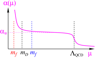
In the presence of , the walking theories may be characterized by as in Fig. 1 which was illustrated in our previous paper Aoki et al. (2013a). This is not fulfilled in ordinary QCD with . The bound states in theories with a coupling behaving as in Fig. 1 are expected to produce “walking signals” based on the following two mass regimes:
-
1.
The approximate hyperscaling relation for the quantities other than holds, , with the same power independent of , , where the SSB effects are negligible. The mass of the pion , as a pseudo NG boson, may have a dependence different than other quantities, as , with . Potentially large corrections to Chiral Perturbation Theory (ChPT), which holds in the general case, are possible. So, even if appears to follow hyperscaling, the validity of it may be restricted to a small region of , or should be different from others. For example, it may change depending on the region of , , reflecting corrections to hyperscaling inherent to ChPT. Thus the hyperscaling for individual quantities—if it is observed at all—is expected to be non-universal.
-
2.
The quantities other than go to a non-zero value in such a way that the hyperscaling relation breaks down or for . On the other hand, (and ) behaves according to ChPT with a chiral log, although the ChPT behavior for the region may appear to mimic hyperscaling with , (up to the chiral log) without a constant term.
In either region the hyperscaling is expected to be non-universal. Thus the simultaneous validity of a ChPT fit and non-universal hyperscaling may be regarded as the “walking signals” to be contrasted with the theory in the conformal window (universal hyperscaling without a good ChPT fit) and that in deep SSB phase such as ordinary QCD (a good ChPT fit and the breakdown of even individual (non-universal) hyperscaling).
I.2 Motivations for lattice studies of large- QCD
In search of a candidate theory for walking technicolor based on the signals described above, there have recently been many lattice studies on large- QCD. See for reviews, Kuti (2014); DeGrand (2016); Aoki (2014); Hasenfratz (2015).333For earlier studies in other contexts, see Ref. Iwasaki et al. (1992) Among large- QCD with a CBZ IR fixed point for , particular interest was paid to the cases of and with staggered fermions, partly because the phase boundary is expected to exist somewhere around , as suggested by the ladder SD equation and the two-loop CBZ IR fixed point mentioned above.
In the case of QCD on the lattice, we obtained results Aoki et al. (2012b) consistent with the conformal window, in agreement with other groups, except for Ref. Fodor et al. (2011) (see DeGrand (2016); Kuti (2014); Aoki (2014); Hasenfratz (2015)). If it is the case, the walking theory should be realized for . It was argued that is also consistent with the conformal window Hayakawa et al. (2011).
How about ? Besides lattice studies to be mentioned below, the theory is of particular interest as a candidate for walking technicolor for various phenomenological reasons. First of all the SU(3) gauge theory with and four weak-doublets () is the one-family technicolor model Dimopoulos (1980); Farhi and Susskind (1981). This is the simplest and most straightforward model building of Extended Technicolor (ETC) Dimopoulos and Susskind (1979); Eichten and Lane (1980), to give mass to the SM fermions by unifying the SM fermions and the technifermions.
Moreover, this same model includes a 125 GeV Higgs as the technidilaton Matsuzaki and Yamawaki (2012a, 2013, 2015): The chiral breaking scale444Our throughout this paper corresponds to MeV in usual QCD. with GeV is much smaller than a naive scale-up of ordinary QCD with , TeV, by the kinematical factor , down to GeV. This is already close to 125 GeV, even without reference to the detailed conformal dynamics, and naturally accommodates a technidilaton as light as 125 GeV by further reduction via the PCDC, , due to the pseudo NG boson nature of the spontaneously broken scale symmetry, similarly to the pion Matsuzaki and Yamawaki (2015). In fact a ladder calculation and a holographic estimate in the one-family walking technicolor yields naturally 125 GeV technidilaton with the couplings consistent with the current LHC data of the 125 GeV Higgs boson.
I.3 Summary of previous lattice results
In previous publications Aoki et al. (2013a, 2014, 2014) we have presented lattice results for QCD indicating salient features of walking dynamics, quite different from those of either our QCD data Aoki et al. (2012b) (consistent with conformality) or our QCD data Aoki et al. (2013a) (indicating a chirally-broken phase similarly to ordinary QCD).
We found Aoki et al. (2013a) walking signals as dual features of spontaneous chiral symmetry breaking and simultaneously of approximate conformal behavior, depending on the mass region and , respectively. In the latter case, the dynamically mass generated by the chiral symmetry breaking was estimated to be around , roughly of order , with (the value of in the chiral limit) being estimated to be based on ChPT.
The former aspect was typically shown from the ratios growing towards the chiral limit , which is consistent with the chiral perturbation theory (ChPT) fit valid for , , , and in a way to satisfy the Gell-Mann-Oakes-Renner (GMOR) relation. Similar behavior was also observed in the Aoki et al. (2013a), and is known to occur in ordinary QCD. These features are consistent with lattice studies of the running coupling in QCD suggesting the absence of an IR fixed point Appelquist et al. (2008); Hasenfratz et al. (2015), though different conclusions are reached in Ref. Ishikawa et al. (2013).
The latter feature, conformality, was demonstrated by the approximate hyperscaling relation valid for , similarly to . However, in contrast to our data Aoki et al. (2012b) with the universal hyperscaling (for ), for all the quantities (ratios between them are constant) in the whole range of , the hyperscaling relation in was not universal, with (a large anomalous dimension, as desired for walking technicolor) for most quantities, with the notable exception of the pion mass , with (namely, more rapidly decreasing than other quantities, or the ratio rising, near the chiral limit as mentioned above). These are in fact the walking signals mentioned before. It was also contrasted to the , where no approximate (even non-universal) hyperscaling relations hold at all.
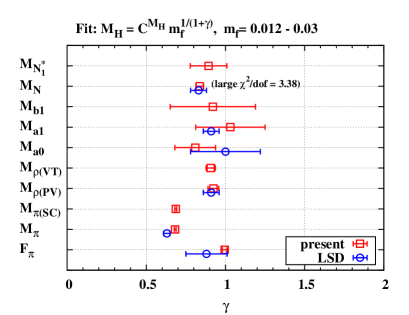
It is remarkable that the LSD Collaboration Appelquist et al. (2014a), using a different lattice action with domain wall fermions, has obtained results similar to ours—in particular, that the ratio grows when approaching the chiral limit. Moreover, the data support non-universal hyperscaling with except for with . Furthermore, recent results by the LSD Collaboration Appelquist et al. (2016), based on nHYP staggered fermions, are also very consistent with ours, with the ratio rising more prominently, up to (compared with our highest ratio ) when getting to smaller .
We further found Aoki et al. (2014) a light flavor-singlet scalar meson with mass comparable to the , . Such a light appear similarly in but Aoki et al. (2013b); Fodor et al. (2014) and is very different from the ordinary QCD case Kunihiro et al. (2004). On the other hand, the lightness of and in contrast to other states, e.g. , in (together with the dependence of growing when approaching the chiral limit) is consistent with the pseudo NG boson nature of both states in the SSB phase. This is in contrast to QCD Aoki et al. (2013b) where their lightness is moderate, e.g. (particularly for large , see also Fig.3 of the latest update Aoki et al. (2015a)), with the ratio being independent of all the way down to the lightest consistently with the universal hyperscaling in the conformal window. It is also remarkable that this light flavor-singlet scalar meson, with a mass comparable to , was confirmed recently by the LSD Collaboration Appelquist et al. (2016) at smaller fermion masses.
I.4 Outline of this paper
In this paper, we present updated results of Refs. Aoki et al. (2013a, 2014). Several preliminary results were shown in Refs. Aoki et al. (2015b, 2016a), together with the latest updated comparison to Aoki et al. (2015a) and Aoki et al. (2016b). We have generated more configurations at with lattice volumes and , for various fermion masses. Compared to our previous results in Refs. Aoki et al. (2013a, 2014), we have added new simulation points in the small mass region and with with 2200 and 4760 HMC trajectories. We have now typically ten times more trajectories than the previous data for small masses. The data analyses in this paper are based on the “Large Volume Data Set” to be shown in Table 2, which includes both new and old data.
We further confirm our previous discovery of a light flavor-singlet scalar, , Aoki et al. (2014), down to the smaller region. Also the above-mentioned characteristic feature of lightness of , i.e., , in contrast to in , now becomes more generic including other states: .
Given the amount of new results we present in this paper, we feel that the reader will benefit from a short summary of different sections. This will allow interested readers to skip to the individual sections knowing what type of analysis we perform there.
In section II, we describe our lattice setup. This section also includes a study of the topological charge history, and the technical measurement details of two-point functions for flavor non-singlet mesons.
In section III we present the results of the hadron spectrum. We first focus on mesonic quantities such as , and . A comparison with the spectrum obtained with the same lattice setup in the and theories is also reported. The main aspects of this comparison include:
-
•
Finite-volume effects are negligible for the largest volume data;
-
•
The taste symmetry breaking effects are negligible similarly to the and in contrast to ;
-
•
The updated ratios of and have a tendency to grow up towards the chiral limit consistently with being in the broken phase as in our previous publication Aoki et al. (2013a). This is in sharp contrast to the data, which tend to flatten near the chiral limit Aoki et al. (2012b, 2015a), but is similar to data, which follow chiral symmetry breaking predictions.
We also show the Edinburgh plot, versus , and similar plots, versus , which compare favorably with the data and the ordinary QCD point.
Section IV is devoted to the ChPT analysis of the hadron spectrum to attempt an extrapolation to the chiral limit. The chiral extrapolation (without chiral logs) of gives a non-zero value . We show that ChPT with this value of is self-consistent, since the expansion parameter is of order . This is in stark contrast to the case of which has . The chiral extrapolation of is non-zero, similarly to the data and consistent with our previous paper Aoki et al. (2013a). We also check the chiral extrapolation of the chiral condensate is non-zero, and coincides with that from the GMOR relation and also from , another version of the GMOR relation.
In this section we also present our full numerical results, including both the updated data of the NG boson pion, flavor non-singlet vector (), and the new data on the flavor non-singlet scalar (), flavor non-singlet axialvector ( with and with ), and the nucleon . Particularly, we give the chiral limit extrapolation of based on ChPT, and the linear extrapolation of the other quantities to the chiral limit, which is relevant to the discussions on the application to walking technicolor, which has . Notable in the chiral limit is that the flavor non-singlet chiral partners tend to be somewhat more degenerate, , closer to the conformal window compared with ordinary QCD, while other chiral partners, , are clearly separated, consistently with the broken phase.
We estimate chiral logs, which are used to evaluate a systematic error on our chiral extrapolation. The final results are , , and . The estimated chiral limit values of and are given in Table X in units of .
In section V we report the hyperscaling analyses we use to test if the theory is in the conformal window. We find that naive hyperscaling holds for quantities such as and with and , respectively, while for it suggests . This non-universality of the anomalous dimension is consistent with our findings reported in a previous paper Aoki et al. (2013a). However, the hyperscaling relation now holds down to smaller masses compared to Ref. Aoki et al. (2013a), where we find it breaking down for . This might be due to the drastically reduced chiral limit value of (and hence as well), so that the crossover point between the hyperscaling validity region and the ChPT validity region discussed in Ref. Aoki et al. (2013a)—if existed at all—may have been shifted to the smaller region in the new data. The non-universal hyperscaling is also seen for other quantities: most quantities show except for which has .
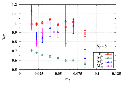
We further estimate the “effective mass anomalous dimension” , which is found to depend on the region, particularly near the chiral limit: the anomalous dimension for gradually increases from 0.6 to 0.7 as decreases, a tendency towards 1.0 which would coincide with the power behavior of the ChPT.
The Finite-Size Hyperscaling (FSHS) relation is analyzed, including systematics for various volume data. The FSHS is reduced to the naive one for the infinite volume limit . First we confirm the FSHS fit for individual quantities separately, similarly to the naive hyperscaling analysis. The non-universality—or the dependence of on the quantity considered—of the FSHS becomes more manifest than in the case of naive hyperscaling, with smaller statistical uncertainty due to the higher statistics by combining data from different volumes. In particular, the FSHS fit to the data is rather bad with and with sharply contrasted to other quantities with . We also check the validity of the simultaneous FSHS with a given universal for different quantities. Taking three typical quantities , the “best fit” is rather bad with and .
To check the possibility that violations of the universality of the hyperscaling are due to being far away from the chiral limit, we also check whether or not the simultaneous FSHS with a given universal for different quantities can be obtained by including possible corrections. The results are given in Table XIII.
Among others, we include the irrelevant operator with the coefficient in the correction factor being the free parameter depending on the quantities and the gauge coupling , which was motivated as a perturbation for Cheng et al. (2014) where was estimated using two-loop perturbation theory. In the case at hand , the perturbative arguments are not reliable and we leave it a free parameter to fit to the data. The results read , which appears reasonable. However, the corrections for are unnatural in the sense that the correction terms does not diminish all the way down to the smallest region due to the small power ,—i.e., they are no longer the mass corrections—and the correction to is particularly large, about 50%. This can be understood as the large corrections changing the divergent behavior of the ratios near the chiral limit into an artificial flat behavior in accord with the universality, particularly near the chiral limit. Thus the universal hyperscaling in various versions does not hold for , in sharp contrast to .
Section VI includes the results for the string tension obtained from the measurement of correlators of Wilson loops. The string tension is measured by fitting the static potential and also via the Creutz ratio. We consider two fits, the quadratic fit , with , and the hyperscaling fit , with . Again we observe the dual features of the walking signals: both the SSB phase and conformal phase with are consistent as far as the string tension alone is concerned. is consistent with the spectrum except for again, non-universal hyperscaling.
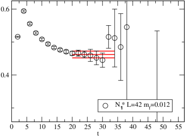
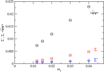
Section VII presents the highlight of this paper, the flavor-singlet scalar , with mass comparable to the pion, which is the updated version of Ref. Aoki et al. (2014). The advantage of the disconnected correlator for extracting the mass is emphasized. We estimate from the disconnected correlator with accuracy better than that from the full correlator, including new data at and partly new data at in addition to the old data in Ref. Aoki et al. (2014) (See Table XIV). The resulting is comparable to (Fig. 23), , which is consistent with the previous one.
As to the chiral extrapolation, we use the leading order of the “dilaton ChPT” Matsuzaki and Yamawaki (2014), , where and (for ), with being the decay constant of the (pseudo) dilaton as , . We use the data for as in Ref. Aoki et al. (2014), which is in accord with the ChPT fit range for other hadrons in Section IV. The fit is . Although the error is so large that no definite conclusion can be drawn at this moment, the value of above is consistent with the identification of the 125 GeV Higgs as the technidilaton in the one-family walking technicolor, with , which would correspond to (using obtained in Section IV).
Section VIII is devoted to a discussion and a summary.
II Lattice simulation setup
II.1 Lattice action and simulations
In a series of studies of SU(3) gauge theory with respect to its properties at many flavors, we have been using the Highly Improved Staggered Quarks (HISQ) Follana et al. (2007); Bazavov et al. (2010) for fermions in the fundamental representation. Our studies intend to explore the theory space from usual QCD to those in the conformal window, passing through the conformal phase boundary. As the correct counting of the light degree of freedom is important for such a study, good flavor symmetry is the first priority in our choice of the action. The HISQ action has been successful in usual QCD simulations Bazavov et al. (2010, 2012) at systematically reducing the breaking of taste symmetry Follana et al. (2007), which is a part of the flavor symmetry. Later in Sec. III.2 we will show the taste symmetry breaking effect in the pseudoscalar meson masses.
A schematic expression of our action reads
| (1) |
with here being the tree-level Symanzik-improved gauge action without tadpole improvement. It consists of the plaquette and rectangular Wilson loops made of the gauge link field . The coupling is defined as ,555This convention is different from the one conventionally used for HISQ simulations in usual QCD, . with being the bare gauge coupling. The fermion part reads
| (2) |
where the number of flavors in this study is for the main result, with additional results for and for comparison. is the staggered fermion field in the fundamental representation of the color SU(3) group, of -th species, with suppressed coordinate and color labels. is the bare staggered fermion mass common for all the species. is the massless staggered Dirac operator for HISQ Follana et al. (2007); Bazavov et al. (2010), which involves one and three link hopping terms where different levels of smeared link of enter, to effectively reduce (but not completely remove) the taste-exchanging one-loop effects. Through this, the flavor symmetry is largely improved. The mass correction to the Naik term is not included as our interest is the system in the chiral limit.
The exact symmetry of this system at non-zero lattice spacing () is the and spin-taste-diagonal axial symmetry for the (one species) case. In the continuum limit the full symmetry of QCD should be recovered. For the and cases, the exact symmetries at are extended to include 666Note that due to the difference of staggered tastes in the conserved vector and axialvector symmetry, and do not simply correspond to left and right chiral symmetry. with the number of species and for and respectively.777Such an extended symmetry is useful, for example, to formulate a method to calculate the Peskin-Takeuchi parameter Peskin and Takeuchi (1990) with staggered fermions Aoki et al. (2016c). Restoring the taste symmetry in the continuum limit leads to the restoration of full symmetry .888The is broken by quantum anomaly.
Eventually we need to understand the dynamics of theory at each in the limit of all fermions simultaneously vanishing , in the continuum and infinite volume limits. For initial steps towards this ultimate goal, we fix the lattice spacing by fixing the gauge coupling Aoki et al. (2013a) for our main calculation in this study, which is . However, we examine the volume and mass systematically to study the infinite volume and chiral limits.
For the study of finite size hyperscaling to test the conformal scenario, it is advantageous to fix the space-time aspect ratio of the lattice, so that the change of the system size is represented by one parameter, which is either for the spatial or for the temporal size for lattice. To this end we use volumes which satisfy for and , while the aspect ratio for is fixed to .
The spatial size for the varies as , 36, 30, 24, 18, and 12. The lattice volume is new here, while the other volumes have already been used either in our study of the flavor singlet scalar Aoki et al. (2014) or in the earlier publication on the “walking signals” Aoki et al. (2013a). Among these, the majority of both the new data set and the ones already used in the scalar study Aoki et al. (2014) have higher statics than those used in Ref. Aoki et al. (2013a). These ensembles, which are more important for this study than the other old ensembles and are called the main ensembles, will be described in detail. For the old ensembles we refer to Ref. Aoki et al. (2013a).
Table 1 shows the statistics of our main ensembles of in terms of maximum number of thermalized trajectories used in this study. shows the number of streams. In the multiple stream cases, shows the total number over all streams. For generating the gauge field ensembles, the hybrid Monte Carlo (HMC) algorithm Duane et al. (1987) with Hasenbusch preconditioning Hasenbusch (2001) is used. HMC parameters, including those related to the preconditioning as well as the molecular dynamics step size, are shown in Table 18. Through all parameter sets the Monte Carlo accept/reject step is placed at the end of each molecular dynamics (MD) integration of unit time 1. Each of such a step is conventionally called a trajectory.
| 42 | 56 | 0.012 | 2 | 4760 |
| 0.015 | 1 | 2200 | ||
| 36 | 48 | 0.015 | 2 | 10800 |
| 0.02 | 1 | 9984 | ||
| 0.03 | 1 | 2000 | ||
| 30 | 40 | 0.02 | 1 | 16000 |
| 0.03 | 1 | 33024 | ||
| 0.04 | 3 | 25600 | ||
| 24 | 32 | 0.03 | 2 | 74752 |
| 0.04 | 2 | 100352 | ||
| 0.06 | 1 | 39936 | ||
| 0.08 | 2 | 17408 | ||
| 18 | 24 | 0.04 | 1 | 17920 |
| 0.06 | 1 | 17920 | ||
| 0.08 | 1 | 17920 |
The MILC code ver. 7 is used for the HMC evolution and measurements on the obtained gauge fields. Some modifications to the MILC code Mil have been made to simulate without the rational hybrid Monte Carlo, which is not needed for the values of we use, as well as to speed up the fermion force computations and so on.
(a) ,
(b) ,
(c) ,
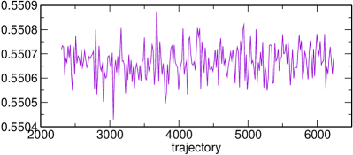
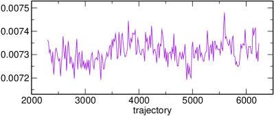
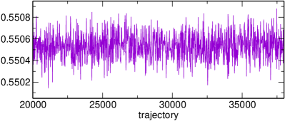
For representative ensembles of the main ensemble set, we show how typical bulk observables change with the Monte Carlo time. The plaquette and chiral condensate are shown for three ensembles: (a) , , (b) , and (c) , in Fig. 2.
(a) ,
(b) ,
(c) ,
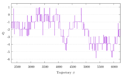
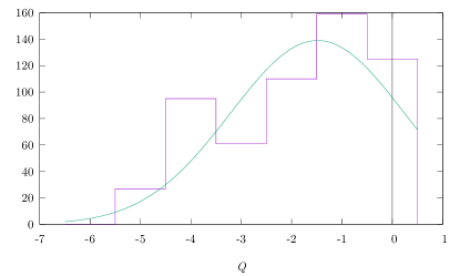
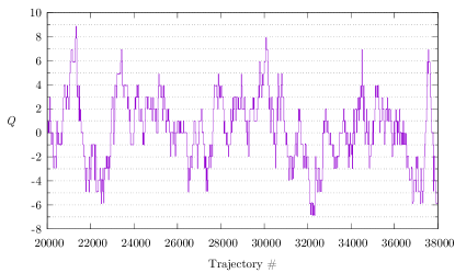
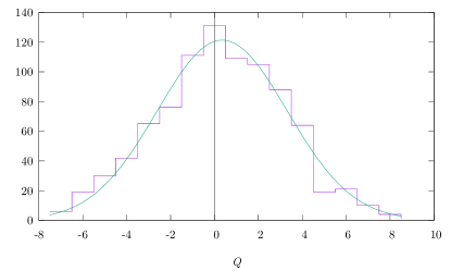
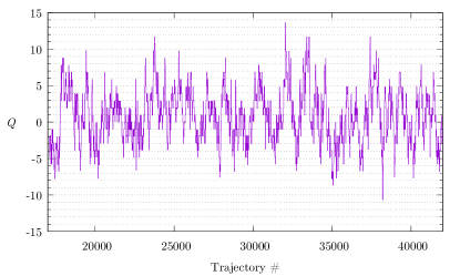
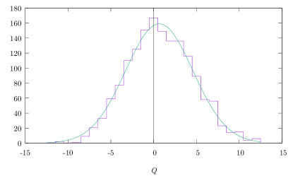
The topological charge typically develops the longest autocorrelation time among the quantities of interest. On the same ensembles used in Fig. 2 the topological change () history and its histogram are plotted in Fig. 3. At the lightest masses () freezing behavior begins to manifest, although it still is moving through the trajectories. Except this lightest mass the topology is moving well and good sampling of topological sectors is observed.
II.2 Extraction of mass and amplitude of composite states
The analysis of the two-point functions of the gauge-invariant composite operators used to calculate the spectrum in flavor-non-singlet channels is described here, with a special emphasis on the staggered-fermion specific definitions and treatments. The case for the flavor-singlet scalar is discussed in Sec. VII.
The generic staggered bilinear operator, which is composed of the staggered and anti-staggered fields in a unit hypercube, reads
| (3) |
where identifies the origin of the unit hypercube, and and are displacement vectors from the origin to any point in the hypercube. and are the spin and flavor (taste) matrices. The details of how these expressions work can be found, for example, in Ref. Gupta (1997). Let us here note that and are species indices, which can take , = , , , where , or for , , respectively. We note that there is a remarkable difference between and , . The bilinear operator in can be made from only one staggered species.
For the flavor non-singlet meson channel we always use operators for and , which prevent the contribution of disconnected diagrams for two-point functions. This “trick” cannot be used for the case. However, as long as the taste non-singlet operators are concerned, we will not include the disconnected contributions. Since the disconnected pieces will not contribute in the continuum limit, omitting them will introduce a lattice artifact which will vanish in the continuum limit, thus is at most, and is further reduced by the HISQ improvement.999In a later section we study the taste symmetry violation effect in the pion spectrum for , which is an example of a similar effect. Let us note that there is a systematic study Bazavov et al. (2012) of the taste violation using exactly the same action, but for real-world QCD (), which is expected to have similar properties as . There a similar lattice spacing as this study is shown to be well in the scaling region and the violation is far smaller than for other actions commonly used.
For the pions we mainly use the exact Nambu-Goldstone (NG) channel,
| (4) |
which is associated with the exact staggered chiral symmetry. The operator reads
| (5) |
and thus is local in , where runs through all the sites including all the corners in hypercubes. The pion mass is measured from the local-local two-point function, with zero-momentum projection. The pion decay constant is measured using the PCAC relation, which holds due to the exact symmetry and correspondence of the continuum and lattice matrix elements Kilcup and Sharpe (1987),
| (6) |
where which is the number of flavors per staggered species. Our pion decay constant is calculated with the matrix element in the right hand side, as
| (7) |
with being the mass of the pion in NG channel. This corresponds to the continuum definition,
| (8) |
where , with or , is the quark mass associated with the flavor . From this expression our pion decay constant can be understood as being normalized with the MeV convention in usual QCD.
The staggered matrix element is calculated from the two point function amplitude at large Euclidean time separation
| (9) |
where , written with the spatial and temporal coordinate separately. The contraction and zero-momentum projection at the source position use a stochastic estimator with single Gaussian random number. In practice we average two-point functions with displaced source time positions in addition to to effectively increase the statistics.101010See for example the column in Table 20, which shows the number of such displaced measurements.
For large time separation, will be dominated by the ground state. With a finite temporal size of our lattice , we often encounter the situation where the ground state dominance is questionable. Therefore we use a method to extend the temporal lattice size in the valence sector to be 2T. The method is combining the fermion propagators with periodic and anti-periodic boundary conditions to make the single fermion propagator for with the sum and with the difference of them. By this the resultant fermion propagator has a periodicity of . As a result, the most distant source-sink separation of the hadron two point function is made to from in the original, which helps to access the range where the ground state dominates (see, e.g., Ref. Blum et al. (2003)). Let be the pion two point function after this manipulation. Its asymptotic form is then given as
| (10) |
with being the mass of the pion in NG channel, whose decay constant is calculated from the amplitude . The effect of the last term, which is constant but oscillating in , is substantial, especially at large number of flavors. The existence of such a term can be understood as follows: the fermion and anti-fermion propagate in opposite direction from the source and meet together at the sink position after one moves through the boundary.111111 For non-staggered (such as Wilson) fermions Umeda (2007), such a wrap around contribution produces a constant term, because the length of the combined fermion lines are constant () as a function of the sink position (), i.e., . It is well-known that such a term exist and the effect is significant in high-temperature (real-world) QCD. Now, noting that the backward propagating fermion will have an opposite parity to the forward one, each one step move of direction of staggered fermion accompanies an oscillating sign. As a result, such a contribution will be proportional to rather than a plain constant. It is easy to see this effect in free field staggered fermions at the NG pion channel, where there exists no staggered parity partner thus no oscillating source exists otherwise. As the number of flavors increases the fermion and anti-fermion are bound more loosely due to color screening.
In practice we eliminate the effect of the -term by taking the linear combination of with the nearest neighbor,
| (11) |
where is restricted to even number, and in this case. The asymptotic form of this correlation function at large is given by
| (12) |
where . In Fig. 4 we show typical effective mass of the NG pion mass at extracted from the two neighboring points and using the asymptotic form Eq. (12).
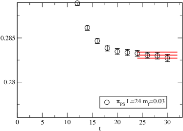
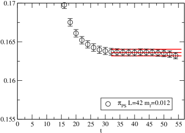
Fitting with Eq. (12) in the range that shows a plateau of the effective mass gives the mass , and the decay constant from
| (13) |
The results are shown in the later sections.
Operators local in a staggered hypercube are always used for the other flavor non-singlet hadrons.121212Exceptions may apply when we study the taste symmetry violation, for which we use all the taste partners of the pion. We examine hadronic channels which couple to the following four operators:
Here conventional QCD state names are used to label the corresponding states in the many-flavor system. In this assignment state(1) always appears lighter than state(2) which is the staggered parity partner of state(1). With fixed time-slice operators the states (1) and (2) always mix Golterman and Smit (1984); Golterman (1986) (see Ishizuka et al. (1994) for a good practical example). The asymptotic form of the zero spatial momentum two-point function reads
| (14) |
where for and are the masses of the state(). In practice in the following sections, state(1) is extracted first with a single exponential fit to (Eq. (11)), which suppresses the effect of state(2), as well as other oscillating components, such as the term in Eq.(10). The state(2) is then extracted from the negatively projected linear combination,
| (15) |
with the contribution of state(1) explicitly subtracted.
For the non-NG and flavor non-singlet state we always use the so-called corner source, where the fermion source vector takes the unit value at the origin of every staggered hypercube and zero otherwise. At the sink position, a zero momentum projection is applied after taking the proper contraction for the staggered bilinear operator. We average two-point functions with displaced source time positions in addition to to effectively increase the statistics here as well.
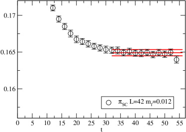
Fig. 5 shows examples of the effective mass of and extracted this way. Similar examples for and are shown in Fig. 6.
For the nucleons we use the local operator with three fermion degrees of freedom on the same point in the staggered hypercube. This operator interpolates the spin state in the 20M, mixed symmetry irrep of SU(4) flavor symmetry, for positive parity and that in the 4A, anti-symmetric irrep, for negative parity. We refer to the former as and to the latter as .131313 The index indicates the fact the lowest state among these is SU(3) flavor singlet in usual QCD. In Refs. Ishizuka et al. (1994); Golterman and Smit (1985) our is named as . Here we adopted a different notation to avoid possible confusion. The nucleon mass is extracted in the same way as the case of non-NG mesons, with a sign oscillation for the backward propagating anti-nucleon signal through the anti-periodic temporal boundary. The typical effective mass is shown in Fig. 7.
III Analysis of hadron mass spectrum
Using the lattice gauge ensembles described in the previous section, we investigate the spectrum of typical hadrons in QCD. We first look at the pion decay constant (), pion mass (), rho meson mass () and the nucleon mass (). We then study finite-volume effects, taste symmetry breaking effects and mass ratios, comparing them with those in and .
III.1 Study of finite-volume effects
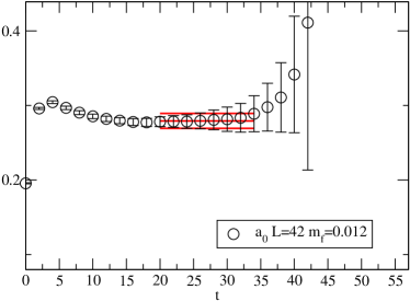
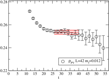
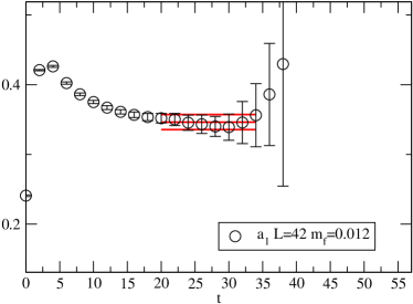
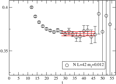
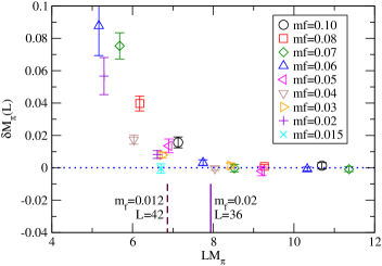
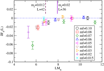
We evaluate finite-volume effects in our lattice gauge ensembles for . To this end, we plot , , and as a function of the lattice volume for each fermion mass in Fig. 8. Here represents the staggered PV vector mass and we will adopt this terminology in the following unless explicitly stated otherwise. As shown in the figure, the spectrum on the largest two volumes is reasonably consistent for all except for which some deviation between the two volumes is seen. We quantify the finite volume effects by using
| (16) |
with being the largest lattice volume at each . Figure 9 shows these quantities as a function of . For , we find (the solid vertical lines); for the somewhat larger masses and , both and become consistent with zero. The finite volume effect for around would be further suppressed, since for a fixed , and tend to decrease with smaller as shown for other values of —for example, around . Such dependences of the finite volume effects may be a consequence of broken chiral symmetry for with regards to the NLO-ChPT prediction Gasser and Leutwyler (1988).
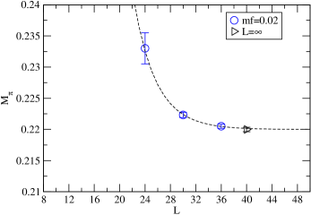
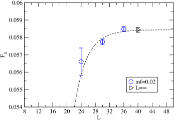
Additionally, we fit the data for and at using the following functions, which are inspired by ChPT Gasser and Leutwyler (1988); Luscher (1986), as in Ref. Aoki et al. (2012b),
| (17) | |||||
| (18) |
where and are the fit parameters of , and and are the fit parameters of .141414 in the fit is fixed to the value estimated from the fit. The fit results are plotted in Fig. 10 as a function of . The figure shows that the largest volume data agrees with the estimated result in the infinite-volume limit within the statistical error. Therefore, we conclude that the finite-volume effects in the data at with are negligible, as is the case for the largest volume data at all other values of .
Data for the spectrum at the lightest fermion mass, , is available for only one volume, , and we estimate its finite-volume effects by utilizing data at the second lightest mass, , shown in Fig. 9. The value of at is highlighted with a dashed vertical line in the figure. Its value is similar to of , where the relative differences and are consistent with zero. Therefore, in the following sections, we assume that finite-volume effects at are smaller than the statistical error. The spectra , , (as well as , which will be investigated in the next section) are summarized in the tables in Appendix C.
In the following sections, we select the spectral data on the largest volumes at each ; the finite volume effects are negligible for them as explained above. Exceptions are made for , , and , where we use the data on the second largest volume, as significantly larger statistics can be utilized. As shown in Fig. 9, the finite volume effects (16) for these data are consistent with zero; the corresponding data points on the figure are the light blue cross (, ), orange right triangle at the rightmost (, ), and blue triangle at the rightmost (, ). From now on in this paper, we shall refer to this data set as the “Large Volume Data Set”, which is summarized in Table 2.
| 42 | 36 | 36 | 30 | 30 | 30 | 24 | 24 | 24 | 24 | |
|---|---|---|---|---|---|---|---|---|---|---|
| 0.012 | 0.015 | 0.02 | 0.03 | 0.04 | 0.05 | 0.06 | 0.07 | 0.08 | 0.10 |
III.2 Taste symmetry breaking effects
We investigate the taste symmetry breaking effects using our QCD lattice ensemble with the HISQ action. For the lattice coupling used in this paper, the taste symmetry breaking in (PS and SC channels) and (PV and VT channels) was shown to be tiny in our previous work Aoki et al. (2013a).
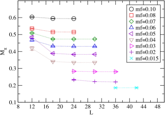
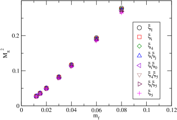
In the present paper, we extend the analysis to include all pion taste partners, . The results are tabulated in Table 3 and shown in Fig. 11; the taste partners are a taste-singlet (), -vector (), -tensor (), -axialvector (), and a taste-pseudoscalar (), where the last one corresponds to the Nambu-Goldstone (NG) pion, . At each fermion mass , the spectra of are almost on top of each other, and thus the taste symmetry breaking is confirmed to be small, consistently with our previous findings Aoki et al. (2013a).
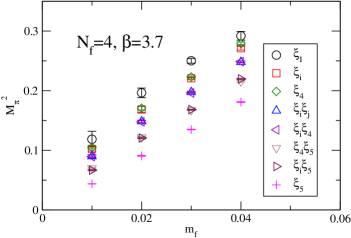
The taste symmetry violation in QCD (Fig. 11) looks quite different from that observed in usual QCD, where much larger taste splitting is typically seen almost independently of Aubin et al. (2004). In contrast to , the taste symmetry breaking in QCD is found to be closer to usual QCD, as shown in Fig. 12. Thus, the tiny breaking of the taste symmetry found in seems to be characteristic of the large number of flavors. In fact, the taste symmetry breaking in (PS and SC channels) and (PV and VT channels) is also tiny in Aoki et al. (2012b).
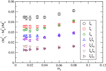
The behavior of taste symmetry breaking becomes more transparent when differences from the NG pion, , are considered. As shown in Fig. 13, the difference is less than 6% in units of . The ratio slightly increases at larger , while approaches to a constant at smaller . This implies that the taste symmetry breaking associated with tends to vanish toward the chiral limit. A similar behavior was previously reported by Lattice Higgs Collaboration Fodor et al. (2009).
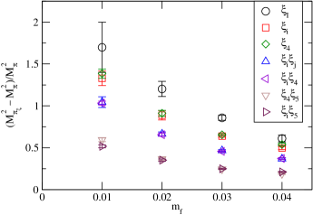
The above features are different from standard knowledge of usual QCD; the taste splitting increases with the lattice spacing, , where is known to be almost independent of in usual QCD Aubin et al. (2004). Therefore the ratio with a “fixed” lattice spacing is expected to diverge as becomes smaller. Such a divergent trend is clearly seen in the case, as shown in Fig. 14, in contrast to . In other words, the lack of divergence in might be a consequence of near-vanishing chiral dynamics. This subject will be further elaborated upon in Secs. IV and V.
However, as we have only one lattice spacing for , from these observations alone we cannot conclude if this apparent difference is due to a difference in the infrared dynamics. We will investigate various hadronic channels in more depth in the following sections. Although we will test only one or two taste partners in each channel, the results in the pion sector here lead to an expectation that the effects of taste symmetry breaking will be small for the mass range we simulate for the theory.
| 0.012 | 42 | 0.1636(4) | 0.1649(4) | 0.1646(4) | 0.1654(4) | 0.1657(4) | 0.1662(4) | 0.1665(4) | 0.1672(4) |
|---|---|---|---|---|---|---|---|---|---|
| 0.015 | 36 | 0.1862(3) | 0.1877(3) | 0.1873(3) | 0.1884(3) | 0.1886(4) | 0.1892(3) | 0.1895(4) | 0.1902(4) |
| 0.02 | 36 | 0.2205(4) | 0.2221(4) | 0.2219(4) | 0.2229(4) | 0.2233(3) | 0.2239(4) | 0.2243(4) | 0.2252(4) |
| 0.03 | 30 | 0.2812(2) | 0.2833(3) | 0.2831(2) | 0.2844(3) | 0.2849(3) | 0.2858(3) | 0.2862(3) | 0.2875(3) |
| 0.04 | 30 | 0.3349(2) | 0.3372(3) | 0.3372(2) | 0.3390(3) | 0.3390(3) | 0.3405(3) | 0.3408(3) | 0.3423(3) |
| 0.06 | 24 | 0.4303(3) | 0.4337(4) | 0.4335(3) | 0.4360(4) | 0.4362(4) | 0.4382(4) | 0.4384(4) | 0.4405(4) |
| 0.08 | 24 | 0.5147(3) | 0.5188(3) | 0.5189(3) | 0.5223(4) | 0.5221(4) | 0.5252(4) | 0.5250(4) | 0.5277(4) |
III.3 Hadron Mass Ratios
The purpouse of this subsection is to give an overview of our hadron spectrum data using ratios of the hadron spectra before carring out fit analyses, which will be discussed in the following sections.
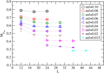
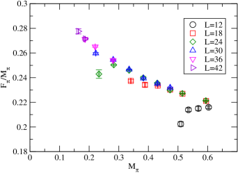
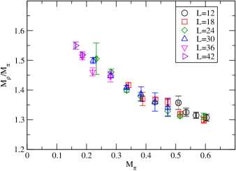
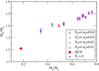
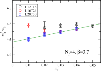
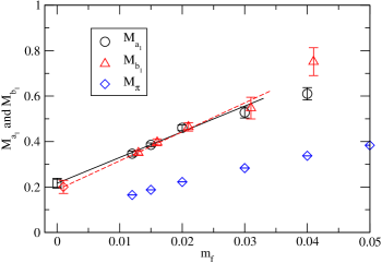
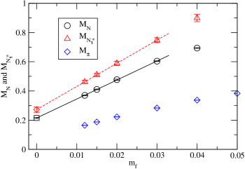
In Fig. 15, we show the ratios and for as a function of for various lattice volumes. Up to some exceptions suffering from finite volume effects, both ratios monotonically increase as decreases. The present results are consistent with our previous work Aoki et al. (2013a) and add larger volume () data in the small region, where we confirm the increasing trend of the ratios still holds. The aforementioned property of is similar to QCD shown in Fig. 16, but different from QCD Aoki et al. (2012b, 2015a). In the latter, the increasing trend ends up with the emergence of plateau at small region.
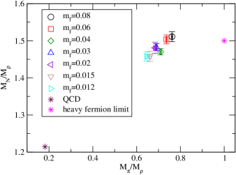
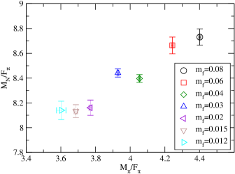
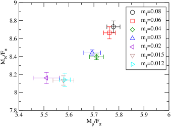
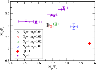
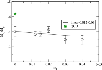
We investigate the ratios of other spectra. The top panel of Fig. 17 shows an Edinburgh-type plot with the Large Volume Data Set, together with the infinite fermion mass limit and the usual QCD point. We find that the data differ from both QCD and heavy fermion limit. The middle panel of Fig. 17 is similar to the top panel, but is used as the denominator of the ratios instead of . In the mass region of , both ratios and show a decreasing trend as becomes smaller, while only the former ratio becomes constant for the smallest three masses, , and ; the pion mass possesses the different dependence in the small region from and . When we replace the horizontal axis in the middle panel with , the pion mass is excluded from both the horizontal and vertical axes. Then, the ratios in both axes () becomes the constant at the smallest three masses (the bottom panel of Fig. 17). This suggests that the dependence of exceptionally differs from the others.
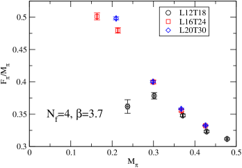
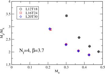
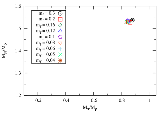
For comparison, we show the versus for with in Fig. 18. The data almost stay at one point, indicating the conformal nature with no exceptional scaling in the spectra. In Fig. 19, we compare the and spectrum data in the Edinburgh type plots. In the upper panel ( vs. ), the data approaches to the QCD point with decreasing , while this is less clear in . In the lower panel ( vs. ), the data points go closer to the QCD point, while the data move in the opposite direction horizontally. Thus, the scaling property of the spectra differs from both those in and .
From the above analyses, we observe that and in QCD have a similar tendency to rise as the chiral limit is approached to QCD, which is consistent behavior with that observed in the chiral broken phase. We also observe, however, that states other than exhibit scaling behavior in the small region. The scaling is similar to the one expected in the conformal phase. In the following sections, we further elaborate the spectra by considering both chirally broken and conformal hypotheses.
IV Chiral perturbation Theory analysis
In this section, we perform polynomial fits using the Large Volume Data Set (as defined in Table 2), under the assumption that QCD is in the chirally broken phase. For this purpose, we focus on the smaller data, . We check the validity of the assumption from the values of physical quantities in the chiral limit, such as , and estimate their values, which would be helpful to predict hadron masses in technicolor models. In the last subsection, we estimate the chiral log correction in ChPT.
IV.1 and
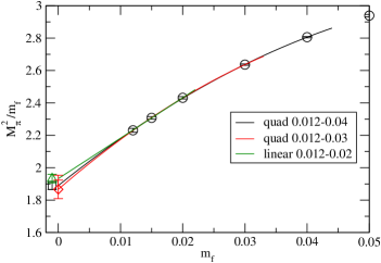
Figure 20 presents the dependence of in the small region. A polynomial fit function is used, defined by
| (19) |
Linear () and quadratic () fits are carried out with several fit ranges, as summarized in Table 4. The fit functions are regarded as NLO and NNLO ChPT predictions of without the chiral log terms. The linear fit function of works well for the three lightest data, while it does not work if the next-lightest data point is included in the fit. The quadratic fit gives smaller dof, and works up to . All the results of in the reasonable fits are nonzero, as shown in Fig. 20. This is a similar property to that observed in our data as presented in Fig. 21.
The expansion parameter of ChPT in flavor QCD Soldate and Sundrum (1990); Chivukula et al. (1993); Harada and Yamawaki (2003) is defined as
| (20) |
and this quantity is required to not be too large, . The values of for the maximum and minimum in the fit are evaluated in each fit result, which are shown in Table 4.
| fit range () | dof | ||||
|---|---|---|---|---|---|
| 0.012-0.02∗ | 0.02612(55) | 3.978(17) | 7.22(31) | 0.43 | 1 |
| 0.012-0.03∗ | 0.02953(24) | 3.111(53) | 9.19(15) | 23.8 | 2 |
| 0.012-0.03 | 0.0212(12) | 6.01(70) | 17.8(2.1) | 0.31 | 1 |
| 0.012-0.04 | 0.02368(54) | 4.84(22) | 20.29(92) | 2.58 | 2 |
| 0.012-0.05 | 0.02435(41) | 4.57(16) | 25.10(85) | 3.00 | 3 |
| 0.012-0.06 | 0.02633(30) | 3.911(90) | 27.02(61) | 14.4 | 4 |
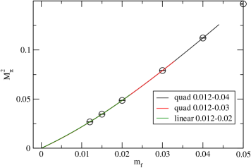
The dependence of is plotted in the top panel of Fig. 22 with the fit function
| (21) |
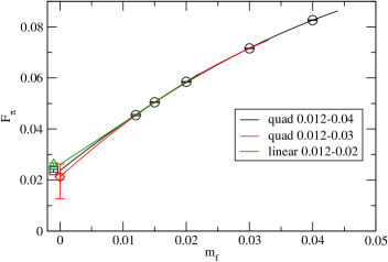
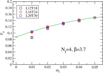
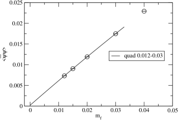
Since the ratio approaches a constant towards the chiral limit, would vanish in the chiral limit. Due to the visible curvature of the ratio, higher order terms than a linear term are necessary to explain our data in contrast to the case, where in the largest volumes at each is reasonably expressed by a linear function of as shown in Fig. 23. The polynomial fits are carried out with several fit ranges, as tabulated in Table 5. The linear fits work in the smaller range, . The quadratic fits give reasonable values of /dof in a wider range, , than in the linear fit. The dependence of and the fit results are plotted in the bottom panel of Fig. 22.
The above analyses for and show that our data can be explained by polynomial functions of , which would be regarded as the ChPT formula without log terms, in the smaller region.
While in our previous work Aoki et al. (2013a) we took the fit results with data for our central values, after accumulating more statistics and including data at even smaller , we choose the quadratic fit results with data, whose values of /dof are reasonable, as the central values in this work. Our central values for and in the chiral limit are
| (22) |
where the errors are only statistical. We will discuss a systematic error of coming from the logarithmic correction in Sec. IV.4. In analyses for other physical quantities as shown in the following subsections, we evaluate their central values with the same range.
| fit range () | dof | ||
|---|---|---|---|
| 0.012-0.02∗ | 1.933(26) | 0.23 | 1 |
| 0.012-0.03∗ | 1.981(12) | 2.13 | 2 |
| 0.012-0.04∗ | 2.0282(83) | 12.2 | 3 |
| 0.012-0.03 | 1.866(57) | 0.04 | 1 |
| 0.012-0.04 | 1.890(24) | 0.12 | 2 |
| 0.012-0.05 | 1.896(18) | 0.12 | 3 |
| 0.012-0.06 | 1.934(13) | 2.57 | 4 |
IV.2 Chiral condensate and GMOR relation
The chiral condensate, , in each flavor is measured by the trace of the inverse Dirac operator, divided by a factor of four corresponding to the number of tastes, as
| (23) |
where is the Dirac operator of the HISQ action. The Ward-Takahashi identity for the chiral symmetry tells us the quantities
| (24) | |||
| (25) |
with being identical to the chiral condensate in the chiral limit , through the Gell-Mann-Oakes-Renner (GMOR) relation,
| (26) |
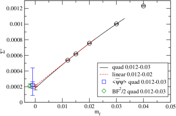
where in the chiral limit, corresponding to in Table 5. In this subsection, we estimate the chiral condensate in the chiral limit from the above quantities using polynomial fits. The dependence for , , and in the small region is shown in Fig. 24.
We first discuss . The data of depend almost linearly on . The linear term in contains a UV power divergence, , which vanishes in the chiral limit. To estimate in the chiral limit, the data are fitted by linear and quadratic functions of , whose results are summarized in Table 6. The quadratic fit result in plotted in Fig. 25 shows that the value in the chiral limit is much smaller than the measured values. This is due to the large linear term. In the smaller region, both the linear and quadratic fits work well, and give nonzero chiral condensate in the chiral limit.
Using the fit results for and in Tables 4 and 5, respectively, we calculate the right hand side of Eq. (26) in each fit range for the two fit forms. The values are compared to the fit results of in Table 6. While in the linear fit result with the smallest fit range the two values are inconsistent, the three quadratic fit results, whose values of dof are reasonable, agree well with those from the GMOR relation.
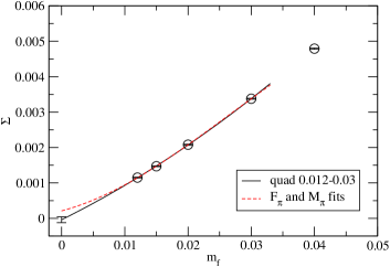
The chiral limit value of is estimated from a quadratic fit in , whose value is consistent with the ones obtained by and as shown in Fig. 26. A linear fit with the range of – also works, and gives a consistent result with the quadratic fit, as presented in the second column of Table 7. The chiral limits of determined by the wider fit ranges give somewhat smaller values than those obtained by Eq. (26). The difference becomes larger as a larger is included into the fit, and would be attributed to higher-order effects.
As shown in Fig. 27 and the fourth column of Table 7, the chiral limit value of is inconsistently smaller than those for , , and . This would not be surprising: as we have seen in the chiral extrapolation of (Table 4), the term is required to perform a reasonable fit of the data in , and thus, and terms would be necessary to capture the dependence of in the same fit range. The quadratic fit lacks such higher-order terms. In other words, even our smallest fit range – would not be small enough for the quadratic chiral extrapolation of . The result in Fig. 27 supports this expectation, as the quadratic fit curve in the smaller region deviates from the dependence of expected from the fit results for and .
Although the extrapolation of has the above difficulties, we observe the consistency among the chiral limits of , , and . Our central value of the chiral condensate is determined from the chiral extrapolation of presented in Table 6, whose value is
| (27) |
where the error is only statistical. A systematic error of the chiral condensate coming from the logarithmic correction will be discussed in Sec. IV.4. The positive value of the chiral condensate is consistent with the property expected in the chirally broken phase. For future work, it is important to confirm that the chiral limit of becomes consistent with the other results by adding more data points in the small region.
| fit range () | dof | |||
|---|---|---|---|---|
| 0.012-0.02∗ | 0.000436(19) | 1 | 0.000330(15) | |
| 0.012-0.03∗ | 0.0005867(84) | 2 | 0.0004319(74) | |
| 0.012-0.03 | 0.000221(43) | 1 | 0.000211(25) | |
| 0.012-0.04 | 0.000255(18) | 2 | 0.000265(12) | |
| 0.012-0.05 | 0.000263(15) | 3 | 0.000281(10) | |
| 0.012-0.06 | 0.000313(10) | 4 | 0.0003352(79) |
| fit range () | dof | ||||
|---|---|---|---|---|---|
| 0.012-0.02∗ | 0.000212(15) | 0.06 | 0.000257(37) | 4.12 | 1 |
| 0.012-0.03∗ | 0.000233(14) | 3.28 | 0.000378(18) | 9.29 | 2 |
| 0.012-0.03 | 0.000183(24) | 0.54 | 0.000039(84) | 1.38 | 1 |
| 0.012-0.04 | 0.000189(15) | 0.34 | 0.000108(45) | 1.17 | 2 |
| 0.012-0.05 | 0.000186(13) | 0.31 | 0.000175(38) | 3.04 | 3 |
| 0.012-0.06 | 0.000206(13) | 3.29 | 0.000159(27) | 2.37 | 4 |
IV.3 Other hadron masses
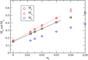
We extrapolate the masses of other hadrons, such as and , to the chiral limit. Since the data for the hadrons have larger error than the ones for and , linear fits work in the small region, , where the quadratic fits for and give reasonable dof. The fit results are summarized in Table 8, and plotted in Figs. 28, 29, and 30.
While and at each are different, the linear fit results coincide within the error as shown in Fig. 28. The near degeneracy of and in the chiral limit was also observed in Ref. Appelquist et al. (2014a). and are almost degenerate at each , and also in the chiral limit, as shown in Fig. 29. This property in the chiral limit is roughly consistent with usual QCD, where and are almost degenerate at the physical . Note that is also almost degenerate to and at each as well as in the chiral limit, as shown in Tables in Appendix D and Table 8. This degeneracy in the chiral limit is a different property from usual QCD at the physical . A similar trend for and is observed in Ref. Appelquist et al. (2016).
We also carry out quadratic fits for all the hadron masses with several wider fit ranges, and find that those results with reasonable /dof are nonzero in the chiral limit. Therefore, all the hadron masses in the chiral limit are nonzero in this analysis, which is consistent with what would be expected for the chirally broken phase.
We investigate the ratio of masses of the parity partners, and . Figure 31 shows that the mass ratio has milder dependence than each hadron mass in the numerator and denominator. The linear fit result of the data in in the figure, as tabulated in Table 8, shows that the ratio in the chiral limit is different from unity, and is smaller than the one in usual QCD, which is 1.636. The parity partners and are expected to be degenerate in the chiral unbroken phase. This property will be discussed in the discussion subsection, Sec. IV.5.
| dof | |||
|---|---|---|---|
| 2 | |||
| 2 | |||
| 2 | |||
| 2 | |||
| 2 | |||
| 2 |
| dof | ||
|---|---|---|
| 1.405(64) | 1.66 | 2 |
IV.4 Estimate of chiral log correction
The logarithmic correction to the chiral fits for and are estimated in the same way as in our previous work Aoki et al. (2013a). In next-to-leading order (NLO) ChPT, the logarithmic dependence in and is predicted Gasser and Leutwyler (1984) as,
| (28) | |||||
| (29) |
where , and and are the low energy constants. Even in the lighter region, the data for both and show no such logarithmic dependences, as shown in the previous subsections.
The size of the logarithmic correction in and is estimated by matching the quadratic fit results to the NLO ChPT formulae at values of such that , with defined in Eq. (20), where should read the re-estimated one in this analysis. The results of the analysis are presented in Appendix E. The correction reduces by about 30% from the quadratic fit, while the effect of the correction is small in .
The results for , , and the chiral condensate at the chiral limit in this work are
| (30) | |||||
| (31) | |||||
| (32) |
where the first and second errors are statistical and systematic ones, respectively. These results including the systematic errors are plotted in Figs. 20, 22, and 26. For all the quantities, the central values come from the quadratic fit with a fit range , and the upper systematic error is estimated from the difference of the central values between the quadratic fit and the linear fit with . The fit results for , in the table), and the chiral condensate are tabulated in Tables 4, 5, and 6, respectively. The lower systematic error of comes from the logarithmic correction in NLO ChPT. For the chiral condensate, the lower systematic error is estimated from the difference between the central value and with the logarithmic correction.
It would be useful to estimate physical quantities in units of , because in technicolor models is related to the weak scale,
| (33) |
where is the number of the fermion weak doublets as . The ratios for all the hadron masses, tabulated in Table 8, to in the chiral limit are summarized in Table 10, where the systematic error comes from the one in . From our result, the ratio in the chiral limit is given as
| (34) |
If one chooses the one-family model with 4 weak-doublets, i.e., in Eq. (33), corresponds to 1.0–1.9 TeV.
IV.5 Discussion
The chiral limit extrapolation of the spectrum of our data in Table VIII indicates non-zero masses with characteristic ratios:
| (35) |
The first relation is a clear signal of the spontaneously broken NG phase, since it is nothing but the famous Weinberg mass relation Weinberg (1967) in ordinary QCD. It follows critically from the inequality of the vector and axial vector current correlators, typically the Weinberg’s spectral function sum rules (SRs)
| (SR1) | ||||
| (SR2) |
combined with the Kawarabayashi-Suzuki-Riazuddin-Fayyazuddin (KSRF) relation . If the chiral symmetry were not spontaneously broken, there would be no pole contribution to the axial vector current and hence term would be missing in SR1; this would imply . SR2 would then conclude —i.e., the Wigner phase, as would be expected in a linear sigma model, with degenerate massive parity doubling; this sharply contrasts with our result .151515In a walking theory there actually is no reason for SR2 to be valid, since yields a slower damping UV behavior of the difference between the vector and axial vector current correlators, instead of in the QCD (where ). The KSRF relation may also change in walking theories, as shown in the Hidden Local Symmetry framework Harada and Yamawaki (2003). Nevertheless Eq. (35)—the same as the Weinberg mass relation—can also follow in walking theories in the NG phase, without recourse to Weinberg’s SR2 and the KSRF relation, as will be described below.
The second relation in Eq. (35) is a novel result also consistent with the broken phase. The unbroken chiral symmetry would be consistent with a linear sigma model for case, particularly when as is the case in our study. The chiral partner should be the parity-doubling flavor-non-singlet pairs —instead of in the case—which are only half of the singlet/non-singlet bound states, excluding the other half . Then the unbroken chiral symmetry created by the parity doubling would imply the degeneracy , in sharp contrast to our result .
To further understand the second relation together with the first one in Eq. (35), we recall the once-fashionable “representation mixing” Gilman and Harari (1968); Weinberg (1969), in which resonance saturation of the Adler-Weisberger sum rule (which is obtained for the spontaneously broken chiral algebra in the infinite momentum frame) occurs. A modern formulation of this method is called “Mended Symmetry” Weinberg (1990), which targets ordinary QCD (and its simple scaled-up version of technicolor, but not walking technicolor). In contrast to our study of large QCD as a walking theory, the analysis in Weinberg (1990) is crucially based on the large limit, with singlet-non-singlet degeneracy (the “nonet scheme”), and the peculiarity of pseudo-real fermion representations, , in such a way that the unbroken chiral partner in the linear sigma model can be identified as . In our case , on the other hand, the chiral partner of is but not the flavor-singlet scalar as mentioned above, although our data for imply that (See the results in the later section).
Consider two one-particle states and , with collinear momenta and , and helicity , respectively. The axial charge in the infinite momentum frame (or equivalently the light-like axial charge), has a matrix element between and which coincides with the Weinberg’s -matrix of axial charge (an analogue of the for the nucleon matrix) Weinberg (1969):
| (36) | |||||
where . Like the nucleon term, the has no pole term (which would have the form ) for the collinear momentum, even in the chiral limit . (The absence of the pole in the corresponding light-like charge was rigorously shown in the original paper of the discrete light-cone quantization Maskawa and Yamawaki (1976), and hence gives well-defined classification algebra, even in the spontaneously broken phase Yamawaki (1998).) On the other hand, the absence of the pole term means that it does not commute with .161616 The current conservation balances the non-pole term, matrix (), with the pole term emission vertex (), which yields the Goldberger-Treiman relation. Namely, the physical states (mass eigenstates) are not in the irreducible representation in general, but in a mixed representation.
For the helicity states, physical flavor-non-singlet meson states fall into four possible chiral representations Weinberg (1969); Ida (1974): For even normality () we have , , while for odd normality () we have and as admixtures of and . Since normality commutes with , we have
| (37) |
which also yields a -independent relation
| (38) |
Thus for the broken phase , we have . More specifically, if “ideal mixing” is imposed in Eq. (37), then setting just reproduces our data (i.e. Eq. (35)).
It is tempting to compare this with our data in Aoki et al. (2013b) (see also the updated results: Figs. 62, 64, 65, and 66 in Appendix G):
| (39) |
Here, all the masses—including —obey the universal hyperscaling relation with , consistent with the conformal window (in contrast to , as will be discussed in the next section). The parity-doubling degeneracy is again badly broken, similarly to , but for a different reason. In the conformal window, there are no bound states in the exact chiral limit ; for this reason, states are often dubbed “unparticles”, and bound states are possible only when the explicit mass exists, so that the chiral symmetry is essentially broken explicitly. The phase is a weakly interacting Coulomb phase where the non-relativistic bound state mass is roughly twice the current quark mass, in conformity with hyperscaling: (see discussions in the Introduction).171717The above mass ratios are in rough agreement with the S-wave degeneracy (up to spin-spin interaction splitting) and P-wave degeneracy , in contrast to . Thus even without spontaneous breaking and the NG pole, the representation mixing should take the same form as Eq. (37). Then the angle-independent relation (Eq. (38) is again expected, and is indeed in rough agreement with data Eq. (39). In this case an alternative Wigner phase known as “Vector Manifestation” Harada and Yamawaki (2003), with (), seems better than the conventional linear sigma type Wigner phase with massive parity-doubling degeneracy, ().
V Hyperscaling Analyses
In the previous section we have performed ChPT based analyses for the hadron spectra and suggested that the system is consistent with being in the SSB phase. In this section we adopt a conformal hyperscaling ansatz as an alternative hypothesis. We highlight characteristic properties of the spectra distinct from those in QCD as well as QCD.
In Sec. V.1, we analyze the spectrum data with the naive hyperscaling ansatz and evaluate a (would-be) mass anomalous dimension (). Next in Sec. V.2, we shed light on the fate of near the chiral limit via the effective mass anomalous dimension () defined as a function of bare fermion mass . Finally in Sec. V.3, we further elaborate the scaling properties of the spectra based on the Finite-Size Hyper-Scaling (FSHS) analyses.
V.1 Hyperscaling Fit
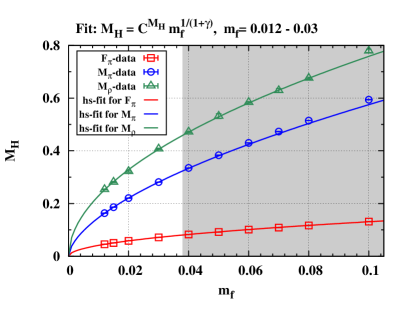
If QCD is in the conformal window, hadron mass spectra should scale as
| (40) |
for sufficiently small in the continuum and thermodynamic limits. The critical exponent is known as the mass anomalous dimension associated with the infrared fixed point (IRFP). While the coefficient may be operator dependent, should be universal. If the system is in the hadronic phase but near to the conformal window, we expect that the scaling law (40) approximately holds with a “would-be” mass anomalous dimension, which may lose the robust universality. This naive expectation is based on past Schwinger-Dyson studies Aoki et al. (2012a) and is supported by our previous work Aoki et al. (2013a).
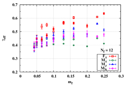
We adopt the conformal hyperscaling ansatz (40), and investigate the same spectrum data set as the previous section (the Large Volume Data Set, Table 2). We first select three observables , , and which were investigated in the previous work Aoki et al. (2013a), and fit their dependences with Eq. (40) for the mass range . Figure 32 shows the three observables as a function of with hyperscaling fit lines. The fit works with relatively small , but is found to be operator dependent: , and for , , and , respectively. The non-universal property of holds for other fit ranges as shown in Table 11. We find that the fit quality for becomes worse significantly for wider fit ranges. Thus, QCD spectra partly show conformal-like scaling but something different from a universal one.
The results explained above are, in principle, consistent with our previous work Aoki et al. (2013a), while there are some modifications to be noted: the hyperscaling ansatz (40) in our previous work failed to explain data in the small mass region, and this trend has disappeared in the present work. The modifications result from the updates in the small mass region; we have added new data point at , and two to ten times larger statistics are accumulated for for which the central values of the spectra have been modified around one percent or less, slightly beyond the statistical errors in several cases. However, the main conclusion in the previous work Aoki et al. (2013a) (the non-universal and the large for ) remains true in the present study independently of the above modifications.
A relevant question is how such a non-universal hyperscaling law has emerged in the spectrum data of QCD. One possibility is that QCD is in the chirally broken phase but the system is very close to the conformal window, and the system still possesses a remnant of the conformal dynamics. Another possibility is that QCD is in the conformal window and the conformal dynamics is contaminated by explicit breaking effects, such as lattice spacing, finite , and lattice volume effects.
| fit range () | dof | ||||||
|---|---|---|---|---|---|---|---|
The and effects will be investigated in the later subsections, and we shall here focus on the lattice spacing artifacts. The important update from our previous work is the collection of from states other than . The results are tabulated in Table 12 and compared with those reported by LSD Collaboration Appelquist et al. (2014a) in the right panel of Fig. 32. In the latter, the domain wall fermion was adopted, in contrast to our choice (HISQ action). Figures show that two different actions result in a consistent with similar observable dependences. This suggests that a non-universal appears independently of lattice spacing artifacts.
| () | ||
|---|---|---|
V.2 Effective mass anomalous dimension
The mass anomalous dimension toward the chiral limit is particularly interesting when considering applications to walking technicolor models. To shed light on the chiral limit from the available data, we investigate the Effective Mass Anomalous Dimension () which is evaluated as follows; first, we divide the fermion mass range of the large volume data set (Table 2) into sub-blocks with sequential three fermion masses, and then, we fit the spectra in each sub-block with the naive hyperscaling ansatz (43). The exponent is determined in each sub-block as a function of , giving .
In the left panel of Fig. 33, we show evaluated from the data set of , , as a function of . Here we also include the nucleon mass . The horizontal axis is the average of the maximum and minimum among three fermion masses in each sub-block. for (green circles) clearly increases with decreasing and it appears to approach , implying the dynamics of the broken chiral symmetry; if a system is in the chirally broken phase, the ChPT predicts , which is identical to . should be contrasted to the results shown in the right panel; for never approaches 1 and all meet at smaller , indicating conformal dynamics with a universal .
The available data for would not be enough to exclude a conformal scenario; there is a possibility that all meet somewhere near toward the chiral limit. In addition, all except for should blow up toward the chiral limit, which would be a smoking gun of chiral symmetry breaking and has not been observed yet. As such, to get more conclusive statement, we need additional data in the smaller mass region, which is considered as a target for future work.
V.3 Finite-Size Hyperscaling Analyses
V.3.1 Preliminaries
We shall now upgrade the hyperscaling ansatz (40) to take account of effects of the finite lattice volume . In many-flavor QCD theories having an IRFP, the fermion mass and the gauge coupling act as relevant and irrelevant operators respectively, in the renormalization group (RG) flow. For a sufficiently small and large , the RG Del Debbio and Zwicky (2010) dictates the finite-size hyperscaling (FSHS) law,
| (41) | |||
| (42) |
At the IRFP () in the conformal window, the function depends on only the scaling variable . The denotes corrections to this scaling, i.e., effects of an irrelevant operator and/or a chiral symmetry breaking. In general, is an arbitrary function of the scaling variable , and in practice, one needs to specify its functional expression. The most probable argument is that the should reproduce the infinite volume hyperscaling formula (40) in the thermodynamic limit (), which indicates the asymptotic formula,
| (43) |
A beyond the asymptotic expression is not well known. If one wants to include a non-linear terms of , one needs some assumption for its expression, which leads to a source of theoretical ambiguities. In this subsection to avoid such ambiguities, we consider only the linear ansatz in Eq. (43). This strategy is based on the following observation; as shown in Fig. 34, the (upper left), (upper right), (lower left), and (lower right), approximately align for , , , and , respectively, and thus linearly depends on up to anomalous behavior at small . This motivates the use of linear ansatz without the small data. In practice, the small non-linearity are excluded by selecting the spectral data with the parameter sets satisfying and with . We refer to the data set as the “FSHS-” Large Volume Data Set, which will be used in the following analyses. Details of the data selection scheme are summarized in Appendix F.2.
By construction, the FSHS-Large Volume Data Set should approximately scale as Eq. (43). This does not necessarily mean the complete conformal nature of QCD since the optimal obtained from the alignment depends on the observable. This will be the focus of the next subsection in terms of the correction terms . For comparison, we show the same figure for in Fig. 35, where the optimal with the alignment shows a much milder dependence on the observables. The comparison to the case (Fig. 36) is also interesting; the and for never show any alignment-like behavior within the unitary band and thus the conformal invariance is completely spoiled by the chiral symmetry breaking. For , the alignment takes place at which is consistent to the leading-order ChPT prediction: .
The FSHS-Large Volume Data Set does not necessarily exclude the spectra with small as long as the linear X dependence holds. This is in contrast to the previous work Aoki et al. (2013a) where the spectrum data with was excluded in the FSHS analysis. As will be shown later, the update of the data selection scheme leads to only a minor modification to the results.
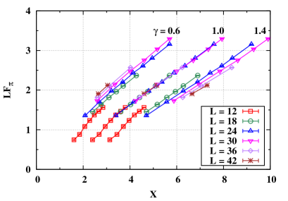
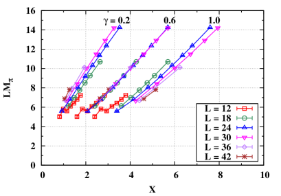
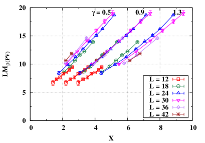
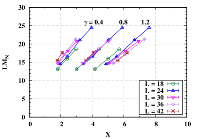
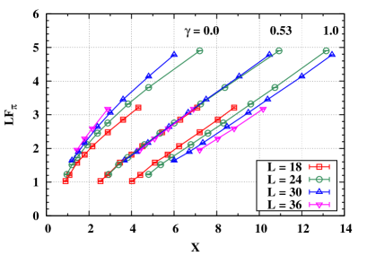
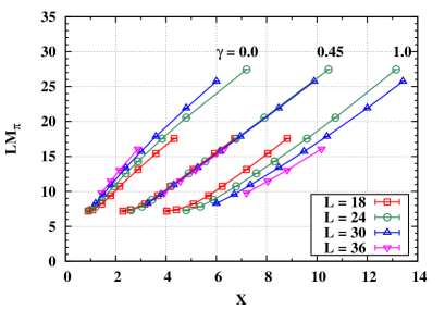
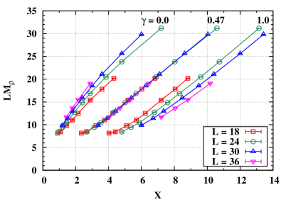
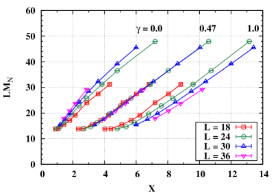
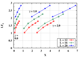
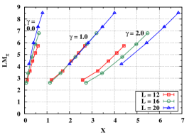
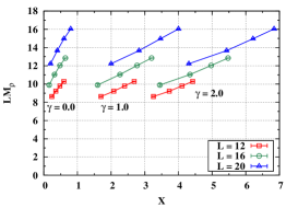
In Fig. 37, we show the value for obtained by the FSHS fit for various quantities. (See Table 13 for numerical details.) The results are similar to those obtained in the naive hyperscaling fits. The observable dependences of remain even in the FSHS with finite volume effects being considered, and rather become manifest with smaller statistical uncertainty owing to the larger number of degrees of freedom. It is also important that the pion mass does not respect the FSHS, as indicated by the considerably large . Thus, the incompleteness of the conformal dynamics seems to be a generic feature of QCD independently of the finite size effects.
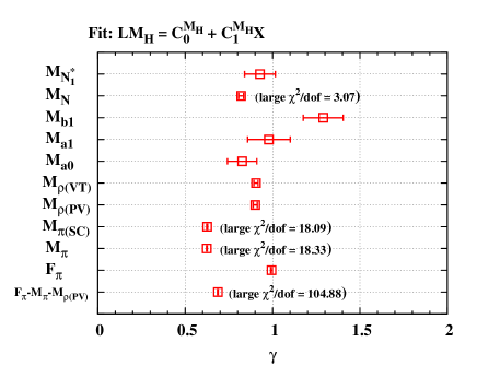
| -- |
|---|
V.3.2 Simultaneous fit with Naive FSHS ansatz
So far, we have investigated the FSHS scaling for each observable individually, and obtained the observable-dependent . We shall now perform a simultaneous FSHS fit, where we construct the combined spectral data including various observables and impose a universal among them. We select the three observables as the combined spectra; the data are available for the widest range from the FSHS-Large Volume data set, and the data quality is better than the other observables. Another practical reason for the choice is that those three observables were used in the previous study Aoki et al. (2013a) and allows us to compare the present result with the previous one.
Our focus is whether the FSHS fit works or fails for a common with or without correction terms . In this subsection and the following subsections, we consider three fit models, , which are summarized in Table 14. Our FSHS fit is carried out in the following procedure;
-
1.
Construct normalized-combined spectral data .
-
2.
We perform fits for the combined data by adopting each ansatz summarized in Table XIV. The would-be mass anomalous dimension () is a common fit parameter. In the models with correction terms shown in Table 14, the second exponent or is also a common fit parameter (For , we consider also fixed cases). In contrast, the coefficients are the observable dependent fit parameters.
-
3.
From each fit, we obtain the and the other fit parameters with . A reasonable fit quality with small indicates the existence of a universal . In this case, if the correction term is much smaller than the leading term , the universal can be identified with the mass anomalous dimension and the system is interpreted to be in the conformal window. As will be shown later (Sec. V.4), this is not the case for .
-
4.
Solve the FSHS formula in terms of the formally:
(44) The explicit form of in each model is summarized in the third column of Table 14. The left-hand side is determined by the lattice parameters and fit results of . The right-hand side is obtained from and results of the fit parameters other than . The fit quality becomes visible in the plane; if a fit model works/fails, spectral data points align/misalign on the line.
| Model Name | ||
|---|---|---|
| Naive FSHS | ||
| FSHS with Power Crr. | ||
| FSHS with RG. Crr. |
In this subsection, we carry out the simultaneous fit with the leading-order FSHS ansatz (43), for which we have,
| (45) |
In the left panel of Fig. 38, we plot the combined data in the plane. The data are scattered around the fit line beyond the statistical errors, and thus the FSHS fit (43) fails: . The result corroborates the lack of a universal .
V.3.3 FSHS simultaneous fit with power-law correction
In Sec. V.2, we have observed the sizable dependence of the effective mass anomalous dimension evaluated from the pion mass spectrum. This is indicative of the necessity of a mass modified FSHS to describe the mass spectra. In this regard, we consider the FSHS ansatz Aoki et al. (2013a, 2012b),
| (46) |
Here, the linear term of can be regarded as the effect of the correction . Among various choices of the second exponent , we consider two possibilities: and . In the former case, the correction term compensates the conformal symmetry breaking due to finite . In the latter case, the correction term accounts for discretization effects.
We show the fit result for in the middle panel of Fig. 38, where the vertical axis is
| (47) |
followed by the definition (44) applied to the present ansatz (46). The figure shows that the data distribute on the fit line and thus the fit quality is greatly improved owing to the power correction term:
| (48) |
We will discuss the interpretation for this result in the next subsection. For , the fit quality becomes better than that in the leading-order FSHS, but still far from the acceptable level: . Thus the lattice spacing correction does not play an important role. This is consistent with what we have speculated in the previous section (Fig. 32) by the coincidence of in different lattice actions.
Here are three remarks in order. First, if we treat the second exponent as a fit parameter rather than a constant, the FSHS fit (46) leads to a successful result:
| (49) |
The interpretation will be discussed in the following subsection, Sec. V.4. Second, the results with the power-law correction explained above are qualitatively consistent to our previous results Aoki et al. (2013a). And finally, we have also fitted using the Schwinger-Dyson (SD) motivated ansatz Aoki et al. (2012a), where the second exponent is fixed as . We find that the over the parameter space contains approximately flat directions due to the parameter redundancy; for example, for , the - and -terms are identical, which gives rise to the flat direction parametrized by . For not far from , the flat direction remains, at least approximately, and prevents us from precisely determining the parameters. Here, we report the rough estimate of the fit result, , for which the fit quality is not of an acceptable level, . When we consider only the spectrum data with in the FSHS-Large Volume Data Set as done in our previous work Aoki et al. (2013a), the result becomes closer to the previous one.
V.3.4 Simultaneous fit by FSHS with RG-motivated correction
If some of irrelevant operators in the RG are nearly marginal, the correction term in the FSHS formula (41) may be dominated by the irrelevant operator . From this viewpoint, we adopt the FSHS ansatz proposed by the recent lattice work Ref. Cheng et al. (2014),
| (50) |
Here, the has been set to be the terms which are responsible for the irrelevant operator . In lattice gauge theories, the operator is the gauge coupling, or equivalently, the lattice spacing effect.
Although the FSHS analyses in the present study do not combine the data computed at different lattice spacings, it is still interesting to consider the ansatz (50) in an alternate formulation. If we assume the -term is dominant and the others are subdominant in Eq. (50),
| (51) |
and rewrite the ansatz (50) within the next-to-leading order,
| (52) | |||
| (53) |
then the expression is analogous with FSHS including power correction term (46). Thus, the ansatz (50) may be regarded as a modified version of (46) with respect to the renormalization group argument.
In contrast to the original work Cheng et al. (2014) for QCD, the value of the second exponent cannot be determined by the two-loop beta function in the present study, since an IRFP does not appear in QCD—at least in the two-loop approximation. We treat as a fit parameter, and thus two exponents are determined by fitting the spectra. As shown in Appendix F.3, we have also performed a global parameter search for , and confirmed that the obtained by the fit realizes the global minimum of .
For the combined data constructed from the FSHS-Large Volume Data Set, the RG-motivated FSHS fit (50) results in the right panel of Fig. 38, where the vertical axis reads
| (54) |
followed by the definition (44) applied to the present ansatz (50). The data points distribute on the fit line with the nice fit quality,
| (55) |
We will discuss the interpretation for this result in the next subsection. The defined in Eq. (53) is found to be
| (56) |
As expected from the similarity between Eqs. (46) and (52), the RG-motivated FSHS results, Eqs. (55) and (56), are almost identical to those in the FSHS with the power-law correction (49).
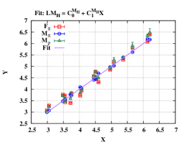
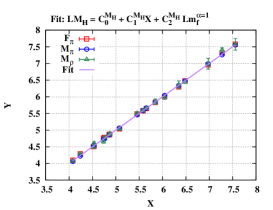
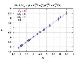
V.4 Discussions
We summarize the mass anomalous dimension obtained so far from the FSHS simultaneous fits in Table 15. The fits have achieved an acceptable for the FSHS ansatz with power-law and RG-motivated corrections. We discuss an interpretation for these results by using the ratio
| (57) |
The ratio quantifies the strength of the correction terms. In Fig. 39, we show the as a function of . The left and middle panels correspond to the cases of the FSHS with power-law () and RG-motivated corrections, respectively. In both cases, the correction associated with pions is considerably larger than those of the other observables. Obviously, only the pion mass possesses a different dependence from the others, which we have already seen as the blowing up of at small (Fig. 15) in the context of the chiral symmetry breaking in the previous section.
For the RG-motivated corrections (middle panel), the correction associated with pions becomes almost fifty percent of the total fit function. The exponent obtained through such a fit would not be regarded as a mass anomalous dimension any more. The same problem potentially exists in the case of the power-law correction term (left panel): the hierarchy of the leading and correction terms are less problematic for , but it increases for the best-fit value of to the same level as the RG-motivated FSHS case.
The above results suggest that the fit has just parametrically absorbed the existing chiral dynamics (the blowing up of ) into the large correction term associated with pion to reconcile the spectra with the universal . In contrast in QCD (the right panel of Fig. 39), the correction terms stay subdominant, and the correction associated with pions is the same order as the others. These are regarded as the distinct properties of the existence of the conformal theory in the chiral limit of QCD.
To summarize, the universal which has been achieved by the correction terms in QCD does not necessarily mean the theory lies within the conformal window, and the analyses of rather implies that the chiral symmetry is broken—though the smoking gun for the symmetry breaking is still missing. It is probable that system is on the border of the chirally broken and conformal phases, and thus QCD is a fascinating theory as a candidate for a walking technicolor model.
| Fit Ansatz | ||
|---|---|---|
| Naive FSHS | ||
| Power Crr. () | ||
| Power Crr. () | ||
| Power Crr. () | ||
| RG. Crr. () |
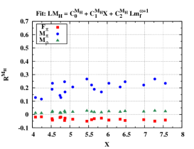
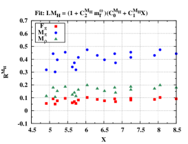
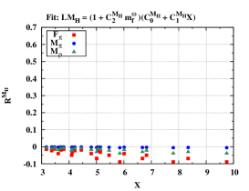
VI Analysis of the string tension
We investigate the string tension between two static quarks in QCD from Wilson loops, using the gauge ensembles stored for the study of the hadron mass spectra. The fermion masses and lattice volumes are selected to include the “Large Volume Data Set” (as defined in Table 2) used in the analyses of the hadron mass spectra. There is one exception: to obtain a better signal, the lattice volume is used for the largest mass instead of , due to the significantly increased statistics available. Finite volume effects are expected to be negligible since the value of obtained for is in the safe region in Fig. 9.
In order to obtain a better signal at large distance, temporal link variables are HYP2 smeared in the spatial direction, and spatial link variables are APE smeared in the spatial direction. We have adopted one of the standard parameter sets (see Refs. Albanese et al. (1987) and Hasenfratz and Knechtli (2001); Della Morte et al. (2004, 2005) for details):
| (58) | |||
| (59) |
We briefly explain the procedure to evaluate the string tension from the measured Wilson loops. Let us consider the potential associated with Wilson loops,
| (60) |
where the represents the Wilson loop with extension , and the bracket indicates taking a jackknife average. For sufficiently large , becomes constant, which is interpreted as the potential between two static fermions,
| (61) |
In Fig. 40, we show the obtained for as a function of temporal extension for the selected spatial extension , , and . In the left panel (), the plateau appears at , and we determine the static fermion potential from a constant fit over the plateau. We repeat the same procedure for the other by keeping the lower edge of the fit range . For a larger , the plateau tends to diminish as seen in the (middle panel) and (right panel) cases, where the statistical uncertainty rapidly increases.
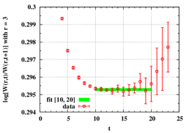
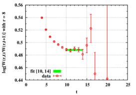
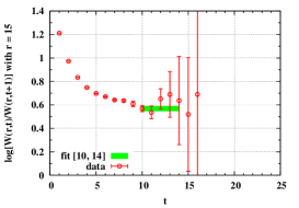
We extract the string tension (in lattice units) by fitting the static potential with the ansatz
| (62) |
with being fit parameters. The static potential for each jackknife bin is fitted separately, to obtain the per-bin string tension, from which we evaluate the central value of the square root of the string tension and its statistical uncertainty . In the left panel of Fig. 41, we show the static potential in the case of . The solid green line represents the fit line for , giving . We repeat the above procedure for various fit ranges over , and select the obtained from the widest fit range for which a reasonable holds. The fits with other ranges give similar values, from which we pick out the largest and smallest string tensions. The differences between the largest/smallest one and the above central value are used to quantify the systematic uncertainty. Data for including both the statistical and systematic uncertainties are summarized in Table 16.
The lower bound of the fit range is set to avoid smearing artifacts. The string tension is responsible for the large-distance behavior of the static potential, while the smearing affects short distance scales. Therefore, one expects that the is independent of the smearing. In practice, however, the fit quality is affected by the smearing artifacts, which prevent a precise determination of . Thus, we need to specify the smearing-free region. To this end, we utilize the Creutz ratio,
| (63) |
The behavior of the Creutz ratio is expressed by using appearing in the potential fit function (Eq. (62)) as
| (64) |
This expression reduces to the string tension itself at . We note that the constant term in the static potential ansatz (Eq. (62)) is sensitive to the smearing, and it has been canceled out in Eq. (64). Thus, smearing artifacts would appear only in the Coulombic term coefficient in Eq. (64) and becomes negligible with increasing .
In the right panel of Fig. 41, we compare the obtained by using different smearing levels in the case of : one (the red squares) is the same as explained in Eqs. (58) and (59), while the other (the blue circles) is 70% as strong; i.e. the smearing parameters in Eqs. (58) and (59) are multiplied by . At , the results of the two smearing levels yield totally different and thus the artifacts dominate. Therefore, we exclude the data at in the following analyses. At , the difference between the two smearings becomes invisible within the resolution of the figure, but still exists beyond the statistical errors. Accordingly, the static potential fit (Eq. (62)) including data gives a large in most cases. For , the two smearings give a consistent within the statistical errors. This holds independently of , and guarantees that the obtained by fitting the data at with the potential fit ansatz (Eq. (62)) should be free from smearing artifacts. The solid green line in the right panel corresponds to Eq. (64) with being specified to those obtained in the potential fit (Eq. (62)). The line agrees with all data at , confirming that the potential fit results and the Creutz ratio data are consistent.
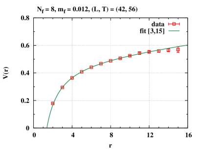
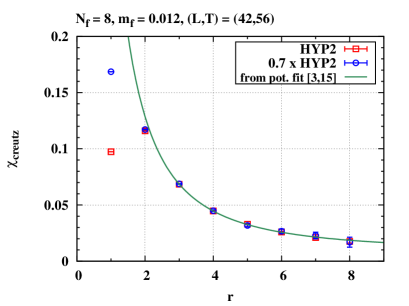
We perform the above procedures at each fermion mass in the range . The results for are summarized in Table 16. In Fig. 42, we plot as a function of fermion mass, with fit lines for the quadratic ansatz and the hyperscaling ansatz . In the fits, only statistical errors are taken into account. The gray (slightly shifted) symbols in the figure are obtained from the data with smaller lattice volumes or statistics and are not used in the quadratic/hyperscaling fits, but are shown to confirm that the finite volume effects are negligible. The fitted parameters are found to be
| (65) | |||
| (66) |
On the one hand, the quadratic fit works well with reasonable and gives a finite intercept of , which implies that chiral symmetry is broken Hasenfratz (2010). On the other hand, the hyperscaling fit also works, and results in the large mass anomalous dimension: . These properties suggest that system is at the border of the chirally broken and conformal phases. It is remarkable that the obtained here is similar to those obtained by the various hadron spectra (Table 12), with the exception of the pion mass case. Although it seems to be difficult to discriminate between the chirally broken and conformal scenarios by the string tension alone, the results are complementary to and consistent with the hadron spectra, and thus support the walking scenario suggested in the previous sections.
| comment | ||||
|---|---|---|---|---|
| not used in fit | ||||
| not used in fit | ||||
| not used in fit | ||||
| not used in fit | ||||
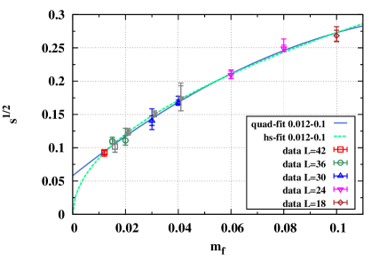
VII Light Flavor-Singlet Scalar Meson
In this section we study the flavor-singlet scalar meson . In the previous sections we have shown that QCD shows signals of walking behavior, being consistent with spontaneous chiral symmetry breaking and also having (non-universal) hyperscaling with . When chiral symmetry is spontaneously broken by the condensate , the scale symmetry is also spontaneously broken by the same condensate in the vacuum. This produces a composite dilaton, the NG boson of the spontaneously broken scale symmetry. In fact, the scale symmetry is also explicitly broken by the dynamically generated mass scale associated with the same condensate, and the dilaton would be a pseudo dilaton having a small mass of order in the chiral limit . In such a case the flavor-singlet scalar meson, as a pseudo dilaton, is expected to be light. In the case of walking technicolor, such a pseudo dilaton, dubbed a technidilaton, may be identified with the 125 GeV Higgs boson discovered at LHC. Thus it is very important to investigate such a possibility of a light flavor-singlet scalar meson in a fully nonperturbative manner on the lattice, particularly for . For this purpose we study the flavor-singlet scalar meson in , and and 4 as well for comparison. In QCD we have found the flavor-singlet scalar mass to be lighter than the NG-pion Aoki et al. (2013b). The existence of a light composite scalar has been observed by several lattice groups with different lattice actions Fodor et al. (2014); Brower et al. (2016). Although the theory is likely in the conformal phase and not a candidate technicolor model, this result suggests that the conformal dynamics may play a role for obtaining a light composite scalar whose properties are quite different from usual QCD. In fact, we have previously measured the mass of the flavor-singlet scalar in QCD on the lattice, and found that the scalar is as light as the pion at the simulated fermion masses Aoki et al. (2014); Appelquist et al. (2016), which could be the first evidence of a candidate for the composite Higgs as a technidilaton, since QCD has been considered as a good candidate for the walking technicolor model. We explore the mass in a region of lighter fermion masses with respect to our previous paper Aoki et al. (2014), so that we can study the chiral behavior of the scalar mass in detail. In the following, we explain the simulation setup and the methods for the flavor-singlet scalar mass measurement, and show the results for the correlation functions, and as a function of . We discuss the chiral behavior of the mass, from which we will obtain the mass in the chiral limit.
VII.1 Measurement setup
We carry out simulations of the SU(3) gauge theory with eight fundamental fermions, and calculate the mass of the flavor-singlet scalar at six fermion masses (=0.012, 0.015, 0.02, 0.03, 0.04, 0.06), on five different lattice volumes . We accumulate trajectories after more than 1,500 trajectories for thermalization. The total number of the configurations as well as the simulation parameters are shown in Table 17.
For the calculation of the two-point correlation functions of the flavor-singlet scalar operator, we use the local fermionic bilinear operator with the taste-spin structure ,
| (67) |
where runs through different staggered fermion species, and summation over a time slice is taken for zero momentum projection. Using this operator, we write the correlator as , where and are the connected and the vacuum subtracted disconnected correlators, respectively. The factor in the disconnected correlator arises from the number of species. To calculate the disconnected piece of the two-point functions, we need the inverse of the Dirac operator for all space-time points. We employ a stochastic noise method with a variance reduction technique based on the axial Ward-Takahashi identity Venkataraman and Kilcup (1997), which has been applied in the literature Venkataraman and Kilcup (1997); Gregory et al. (2008); McNeile et al. (2013); Jin and Mawhinney (2011). We use 64 random sources spread in spacetime and color spaces for this noise-reduction method. For staggered fermions, the interpolating operator in Eq. (67) can also couple to the state with , which is the staggered parity partner of , a flavor non-singlet pseudoscalar. The asymptotic behavior of the correlators of the flavor-singlet scalar is given by
| (68) |
where , and the state is a species-singlet pseudoscalar with taste-spin structure . The connected piece behaves as
| (69) |
where the states and are the flavor non-singlet scalar and the flavor non-singlet species non-singlet pseudoscalar, respectively. Then the disconnected piece can be written as
| (70) |
If the flavor symmetry is exact, the masses of both the flavor non-singlet pseudoscalar and are degenerate, and their amplitudes coincide; this means , since the disconnected piece of the flavor non-singlet channel disappears in the taste symmetric limit. The contribution of the opposite parity state in the staggered fermion can be suppressed by applying the positive parity projection, at even . Another projection at even is also defined to maximize the opposite parity contribution .
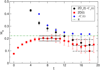
A typical result for and is shown in Fig. 43. In the figure, behaves as a smooth function of in contrast to , which has an oscillating behavior. This result means the taste symmetry breaking effect on and is negligible in the parameter region we simulate. The effective masses of , , and are shown in Fig. 44. Since the combination at large is dominated by , the effective mass of the at large becomes consistent with the one obtained from . An advantage of using in extracting is that that the plateau of appears at earlier than that of the , which enables us to determine with better accuracy. This earlier plateau happens to appear in the mass parameter we simulate, which might be caused by a reasonable cancellation between the contributions of and excited states of . It is also shown that the effective masses of as well as are smaller than that of , as plotted in the figure. Due to the smallness of compared to other hadron masses, the exponential damping of is milder than that in usual QCD. It helps to prevent the rapid degradation of the signal-to-noise ratio.
We fit with the assumption of a single scalar propagation. The fit range is for all the simulation parameters for which we find an effective mass plateau. In order to estimate a systematic uncertainty coming from the fixed fitting range effect, we also fit with a later region, with the same number of data points, as shown in Fig. 44. We quote the fit result with fixed range as a central value, and estimate a systematic error as the difference of the values obtained by differing fit ranges. All the results are tabulated in Table 17. It should be noted that, in somewhat smaller mass region, an additional effective mass plateau seems to appear at later region, whose mass is below the one obtained in the region at small . In the later time region, however, the effective masses are not stable, with larger error in , so that more data are required for a better identification of the ground state mass. We find that the results with two different fit ranges are consistent with each other except for , whose result is shown in Fig. 45.
While in the current analysis we determine from the earlier plateau of , and estimate the systematic error from the later one, a more reliable result can be obtained from a plateau of the full correlator , if the statistics is sufficient to obtain a clear signal in the large region. Therefore, it is an important future work to compare our results with the ones from more reliable calculations with much larger statistics to examine whether our determination of is reasonable or not.
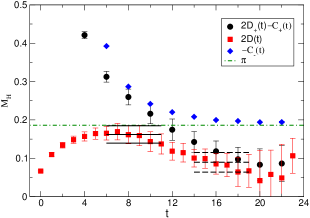
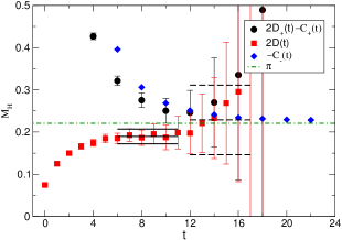
| [] | ||||
|---|---|---|---|---|
| 0.012† | 2300 [2] | 0.151(15)() | ||
| 0.015∗ | 5400 [2] | 0.162(23)() | ||
| 0.02 | 5000 [1] | 0.190(17)() | ||
| 0.02 | 8000 [1] | 0.201(21)() | ||
| 0.03 | 16500 [1] | 0.282(27)() | ||
| 0.03 | 36000 [2] | 0.276(15)() | ||
| 0.04 | 12900 [3] | 0.365(43)() | ||
| 0.04 | 50000 [2] | 0.322(19)() | ||
| 0.04 | 9000 [1] | 0.228(30)() | ||
| 0.06 | 18000 [1] | 0.46(7)() | ||
| 0.06 | 9000 [1] | 0.386(77)() |
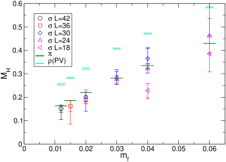
VII.2 Chiral extrapolation
The scalar is as light as in our fermion mass range. Fig. 46 shows the results for the scalar mass compared with and . To estimate the impact of finite size effects, we show the values of in Table 17. As we see, the data at the largest two volumes are consistent with each other for . An estimate of suggests that the finite size effect on is negligible in the data with , so that finite size effects for and , where only a single volume is available, are inferred to be negligible in our statistics.
First we would like to study the chiral behavior of from dimensionless ratios of spectral quantities. Fig. 47 shows as a function of on the largest volume at each mass. For reference, we also plot these quantities in QCD with as a candidate for the lowest scalar bound state. The ratio has a mild dependence at smaller fermion masses, and its value is close to the one in usual QCD, while there are large statistics and systematics uncertainties.
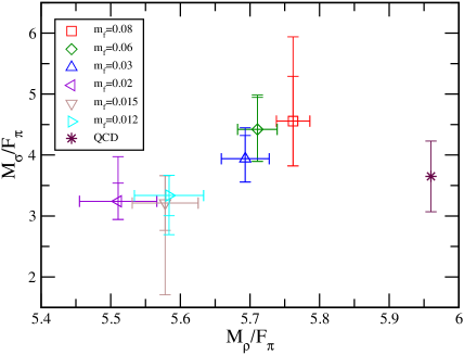
Assuming this theory is in the chirally broken phase, we discuss the chiral limit extrapolation of . While we have a light scalar with mass comparable to , the validity of chiral perturbation theory is intact by introducing a dilaton field which is a pseudo Nambu-Goldstone boson of the scale symmetry (“Dilaton ChPT” (DChPT) Matsuzaki and Yamawaki (2014)).
Treating the light scalar as a dilaton field in the effective theory is, in general, just a particular assumption for its potential and possible interactions. However, for a vector-like gauge theory, such as the one we study here on the lattice ( QCD), there cannot be a light flavor-singlet scalar other than a dilaton. The global symmetry breaking patterns in the chiral limit of vector-like gauge theories, dictated by the Vafa-Witten theorem, are of the symmetric coset G/H Kosower (1984); Peskin (1980), none of which has a NG boson scalar that can be identified with the SM Higgs. In fact, NG bosons in the symmetric coset G/H have no odd-numbered vertices, such as “3-pion” vertex (see e.g. Ref. Bando et al. (1988)), and cannot decay into a pair of other NG bosons in the same coset G/H (which we usually think to be absorbed into W/Z). Thus such NG bosons in the symmetric coset cannot be identified with the 125 GeV Higgs, which has been established by the LHC experiments to decay into a pair of longitudinal W/Z bosons Aad et al. (2015); Khachatryan et al. (2015).
To find a workaround for the Higgs to W/Z coupling and still identify the light scalar Higgs as an NG boson of the same G/H as those absorbed into W and Z bosons is not an easy task. A UV completion for such a G/H is only realized in chiral gauge theories in accord with the Vafa-Witten theorem which is crucially based on the positivity of measure in the lattice regularization. Patterns of symmetry breaking in chiral gauge theories, however, have only been analyzed by the most-attractive-channel (MAC), a perturbative one-gauge-boson exchange picture. A full nonperturbative treatment on the lattice is not available yet. (Moreover, a chiral gauge theory is a necessary condition, but not a sufficient one, to avoid the symmetric coset, which is remains still a possibility, e.g., , in chiral gauge theories, although symmetric coset in chiral gauge theories could be viable under more involved assumptions such as the vacuum misalignment to develop the Higgs VEV, etc.)
We therefore proceed our chiral extrapolation analysis of the light flavor-singlet scalar mass using DChPT. At leading order in DChPT, the mass is given by
| (71) |
where , and . The is an effective mass anomalous dimension in the walking regime, and and are the decay constants of and in the chiral limit, respectively.
In the following fit analyses, we shall use the lightest four data points () with the leading order dilaton mass fit function. We carry out the fit with a data set in which all the four data are chosen at the largest volume with the fixed range, and obtain a result as a central value. The effect of the systematic errors in is taken into account in the chiral extrapolation fit by varying the data set used. We consider all the combinations of the data set where each of the data is chosen as the result from the first fit range or the second one. Thus we have in total sixteen data sets for the lightest four fermion masses. We carry out fits for all the data sets, quoting the maximum difference of as a measure of the systematic error due to the choice of the plateau in the effective mass. Each chiral extrapolation is performed with the statistical errors only. The fit results are shown in Fig. 48. The fit of the chiral extrapolation gives a reasonable dof=0.40, and the value of in the chiral limit , where the first and second errors are statistical and systematic, respectively. Thanks to a higher precision of this result compared to Ref. Aoki et al. (2013b), we now obtain a value of closer to zero. From the linear slope , we can read off the value of . The DChPT fit gives . If the effective mass anomalous dimension is , we can obtain with , which is consistent with another calculation of the dilaton decay constant via the scalar decay constant and the Ward-Takahashi identity of the scale transformation Aoki et al. (2015b). It is also noted that the result for is quite different from usual QCD, where a larger slope is observed for MeV Kunihiro et al. (2004).
We can also fit with an empirical form, , using the same data set. The fit result is shown in Fig. 49. The chiral fit of also gives a reasonable dof , . This result is consistent with that of DChPT. Although our result for the scalar mass has a sizeable error, and the chiral limit is probably far from our current simulation regions, both the fit results of and suggest the possibility to reproduce the Higgs boson with mass GeV via a scale setting of GeV in the one-family technicolor model with four weak-doublets. We have estimated a small value of in the chiral limit, so that a small value of would be required to be consistent with the composite Higgs in the one-family model. Using the fit result for , we obtain in the chiral limit. Thus the value of is comparable to even in the chiral limit, while the error is large. This result is encouraging for obtaining a composite Higgs boson with mass GeV.
We note that the hyperscaling fit in the conformal hypothesis, , works in the smaller mass region. The fit result is shown in Fig. 49. The conformal fit gives a /dof , and . This should be compared with the result in the right panel of Fig. 32. This behavior—that both the fits of the (D)ChPT and hyperscaling with a large mass anomalous dimension work in an appropriate mass region—matches the one seen in the spectra of other hadrons. It is quite different from usual QCD and could be a signal of the walking gauge theory. An important future direction is to obtain a precise value of in the chiral limit, which will be useful to study if this theory really exhibits the desired walking behavior, and reproduce the Higgs boson with GeV mass. For this purpose, we need more data at lighter fermion masses with larger volumes.
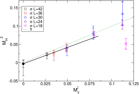
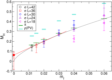
VII.3 Dilaton decay constant calculation
From a phenomenological point of view, the technidilaton decay constant (denoted here as ) is an important parameter, since controls all the technidilaton’s couplings to SM particles.
The dilaton decay constant is defined as , from which we also obtain . Therefore the dilaton decay constant can be directly calculated from the matrix element of the dilatation current. However, the dilatation current is rather difficult to construct on the lattice, since it contains a power divergence that needs to be subtracted. Instead, we consider an alternative way to estimate it from a relation between the scalar decay constant and obtained in the continuum theory. Here the scalar decay constant is defined as the scalar operator matrix element,
| (72) |
where is the flavor-singlet scalar bilinear operator . Thus the above matrix element can be calculated from the two-point correlation function () on the lattice. We note that this quantity is renormalization group invariant and a physical quantity. Following the argument based on the continuum theory Bando et al. (1986), we obtain a relation
| (73) |
where is the scaling dimension of and total number of fermions.181818 This relation can be derived by using the Ward-Takahashi relation for the dilatation current in the continuum theory. For the detail of the derivation, see Aoki et al. (2015b). (Dividing both sides by leads to the relation obtained at Matsuzaki and Yamawaki (2012a).)
We note that this relation holds in the continuum theory with infrared conformality by saturating the Ward-Takahashi identity for the dilatation current by the single pole dominance of as a dilaton in the spontaneously broken phase of the scale symmetry, as well as the chiral symmetry. We here assume that this relation remains valid also on the lattice up to discretization effects, in the same spirit as our analysis of and using Eq. (71). The method here is a semi-direct estimate of alternative to that based on Eq. (71).
The result for is summarized in the left panel of Fig. 50, where we obtain a signal for as the same statistical accuracy as the mass. We estimate a systematic uncertainty coming from the choice of fitting range, which is also shown in the figure. On the right panel of Fig. 50, the result of from the semi-direct estimate Eq. (73) is shown. For the chiral condensate, we use its chiral limit value to avoid large lattice artifacts. We also carry out chiral extrapolation fits, whose results are also shown in the figure. In the chiral limit, we obtain . Given that , we have shown how two different methods, DChPT (Eq. (71)) and this method, give a consistent result for .
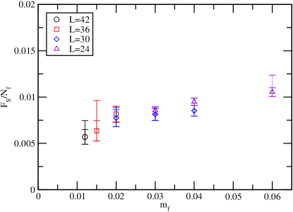
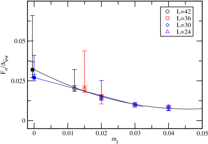
VII.4 Phenomenological implications for dark matter physics
One interesting phenomenological implication of the measurement of is an application to dark matter (DM) direct detection. In technicolor models, there is a good candidate for composite DM: a neutral baryonic bound state made of constituent (possibly charged) technifermions. As shown below, the coupling between SM particles and the DM as well as the mass of the DM are constrained by direct detection experiments. The scattering rate of DM with heavy nuclei in detectors is an important parameter for experiments, a dominant contribution to which is the Higgs (scalar)-mediated spin-independent process. Using we discuss the detectability of DM from that process.
We consider a DM effective theory including a dilaton, based on DChPT Matsuzaki and Yamawaki (2014). Since the DM is the lightest technibaryon, the extension to the baryon sector of the DChPT is straightforward. In the leading order the dilaton field can only couple through the nucleon mass term as
| (74) |
where , is the baryonic DM field, and is its mass in the chiral limit. The parameter explicitly breaks the scale symmetry, and the (pseudo) dilaton acts on this term to make the action scale invariant. Then the dilaton-DM effective coupling () is uniquely determined as . Regarding to the SM sector, we also use the dilaton effective theory Matsuzaki and Yamawaki (2012b) to determine the coupling of and a target nucleus. Combining both SM and technicolor sectors, the cross section with a SM nucleus for the spin-independent part is given as , with , where is the mass of the target nucleus, and and are the total number of the protons () and neutrons () in the nucleus ( is the mass number). The parameter is defined as , where is the nucleon -term of the light quarks (), and is that of the heavy quarks.191919 It is possible that technifermions can be charged under SM color, so that there may exist additional contributions to the nucleon -term from the technifermions. In this analysis, we omit these contributions for simplicity.
Here we show our numerical results of the DM cross section.202020 A similar analysis on the lattice has been performed for a different composite DM model based on strong dynamics Appelquist et al. (2014b). We use the lattice results of the dilaton decay constant obtained from the previous section and nucleon mass, while the scalar mass is fixed to its experimental value ( GeV) in this analysis. To set the scale, we use the relation GeV. To compare with experiment, we use the cross section per nucleon () instead of , which is defined as . The result is shown in Fig. 51. According to DM direct detection experiments (see e.g. Akerib et al. (2014, 2016); Tan et al. (2016) for recent experimental results) our values for are excluded under the assumption that the technibaryon is the major component of the dark matter relic density.212121See Ref. Fodor et al. (2016) for a similar example in the context of composite baryonic dark matter. We note that there exist other contributions to the DM cross section, e.g. gauge boson mediated interaction, and higher order terms, which might affect the DM cross section. It would be interesting to investigate these contributions.
VIII Summary and Discussion
In QCD with , we have confirmed the general structure of the walking signals in the spectrum observed in our previous results Aoki et al. (2013a), with dual features such as satisfying both ChPT and (non-universal) hyperscaling relations. We have also confirmed the outstanding discovery of a light flavor-singlet scalar , with mass comparable to that of the pion Aoki et al. (2014), extending the studied parameter space down to and to the larger volume . We have studied more spectral quantities, including , , and , in addition to those presented in Refs. Aoki et al. (2013a, 2014) (namely , , and ), with higher statistics. Typically ten times as many trajectories as the previous data were used, for all but the .
We paid particular attention to the systematic comparison of the data with our data (shown to be consistent with the conformal window) and data (consistent with SSB phase without remnants of conformality) obtained with the same lattice setup.
We performed a ChPT analysis of and for with the estimate of the chiral log used to evaluate the systematic error:
| (75) | |||||
| (76) |
which is consistent with the GMOR relation in the SSB phase. The chiral limit value of mass in units of is .
On the other hand, the hyperscaling relation holds in various intervals of , including the lightest , with for all the quantities (including the string tension) as anticipated for the walking technicolor. A notable exception to this is , for which hyperscaling is valid only in a restricted range of masses (see Table 11), and Finite-Size Hyperscaling (FSHS) (cfg. Fig. 37) gives with a large . This is consistent with the NG-boson nature of , whose mass obeys the ChPT relation (see Eq. (21))
| (77) |
which would imitate the hyperscaling relation only locally—in a very narrow range—such that for larger with , and for smaller with , in perfect consistency with the -dependence of for (see Fig. 33). The average result is just in between these two extremes, showing a sharp distinct behavior of compared with all other quantities. This is also compared with in Fig. 33. Overall, a characteristic hyperscaling fit of our data gives:
| (78) |
Thus we find that the hyperscaling relation in is non-universal, for both the naive hyperscaling and the FSHS (see Fig. 33 and Fig. 35). This is in sharp contrast to where we find near universal hyperscaling with , including . It addition, the ratio of quantities with respect to , such as , is increasing even at the smallest (), without indications of plateaux. This trend is not observed in , while it is a characteristic of ratios.
The result is also contrasted to the data where all the quantities but do not obey the hyperscaling relation at all. They have no remnants of conformality, while only imitates the hyperscaling with , which is actually nothing but the ChPT formula with (see Fig. 36).
We further confirmed our previous discovery of a light flavor-singlet scalar, , Aoki et al. (2014), even at smaller . Also the hierarchy of masses , in contrast to in , now became more generic including other states:
| (79) |
The chiral limit extrapolation value using dilaton-ChPT Matsuzaki and Yamawaki (2014) is more consistent with the identification of with the 125 GeV Higgs than the previous one, with improved error bars and a central value closer to zero.
Although we observed data consistent with ChPT for , with , the region we studied seems to be still too far from the chiral limit to establish whether the theory is in the SSB or the conformal phase, if the data are analyzed in isolation from and data. We found no decisive evidence for the SSB phase, such as the chiral log effects in ChPT and the obvious breakdown of the hyperscaling (or divergent for spectrum other than ) as we expect in .222222The Pagels-Stokar formula, together with the SD equation, implies for , while may be estimated as –0.16 (See Tables 8 and 21–26). It is clear that our data are not in the near chiral limit where . Nor did we observe any clear evidence of the conformal phase: i.e., the hyperscaling, if existed at all, is not universal—in particular for —and is increasing down to , in contradiction to what is expected in the conformal phase. In addition, we observed no near degeneracy of the chiral partners, , , in contrast to our expectation for the conformal phase without SSB.
Although the decisive conclusion has yet to be drawn about the discrimination between the SSB and the conformal phases, what we observed is fairly consistent with expected signals of a walking theory: having light and as pseudo NG bosons, and being in the SSB phase (as indicated by the ChPT fit) together with remnants of the conformal window (non-universal hyperscaling and non-degeneracy of the chiral partners), sharply distinct from our data for the theory (definitely consistent with the conformal phase and in disagreement with the SSB phase), and those on the which obviously signal the SSB phase.
As we noted in Ref. Aoki et al. (2014), if is the pseudo dilaton, then is expected to become bigger than when we get to near the chiral limit, . This is because as a pseudo dilaton would have chiral limit mass due to the trace anomaly generated by , as was mentioned before, and is estimated to be Matsuzaki and Yamawaki (2015) of order for . It is also phenomenologically crucial to have this chiral limit behavior in order for to be a viable candidate for the 125 GeV Higgs in walking technicolor with .
In this sense the recent LSD results Appelquist et al. (2016), in a region of smaller than ours, show a similar tendency: , but not , suggesting we may still be some distance away from the chiral limit. Data at even smaller are needed to further establish the chiral behavior of .
All the couplings of the technidilaton as a composite Higgs are described by the effective field theory respecting all symmetries of the underlying theory. In the case at hand—the walking theory—these are the chiral and scale symmetries. Possible explicit breakings such as effects and the trace anomaly are also controlled in terms of the spurion fields. The relevant effective field theory is dilaton ChPT Matsuzaki and Yamawaki (2014) as a straightforward scale-symmetric extension of conventional ChPT. (See also Matsuzaki and Yamawaki (2015) and references therein.)
The “Higgs potential” for the dilaton field is uniquely determined by the trace anomaly in terms of just two parameters and :
| (80) |
where transforms as ) under scale transformations, and so does the spurion field (), hence in accordance with the PCDC in the underlying theory. Thus measuring as well as on the lattice determines completely the Higgs potential for the 125 GeV Higgs as the technidilaton. Also all the couplings to the SM particles are determined by (up to some nonperturbative contributions to the couplings of the technidilaton with the SM gauge boson pairs).
From the lattice data on the mass through Eq. (71) based on dilaton-ChPT, we can read off not only the chiral limit value of given by but also the decay constant from the slope (for ).
Our data suggest that from . A similar result has also been obtained by a different method Aoki et al. (2015b). In the case of the one-family model, this would imply , which would be somewhat smaller compared with the favorable value (for ) for accounting for the LHC 125 GeV Higgs data Matsuzaki and Yamawaki (2012a). Considering that our data have significant uncertainties and are still far from the chiral limit, however, it may be a bit premature to draw a definite conclusion for phenomenology. Particularly, we should look at the relevant slope as well as in the region where , which is not available in our present lattice setting.
The parameter Peskin and Takeuchi (1990); Holdom and Terning (1990); Golden and Randall (1991) is usually a challenge for the walking technicolor based on the large QCD, since the large factor (more precisely, a large number of electroweak doublets if all flavors carry the electroweak charges) enhances the parameter from the pure technicolor sector at least in perturbative calculations and/or a simple scale up of QCD.232323 However, the large parameter from the technicolor sector as it stands is not necessarily in conflict with the experimental value of the from the electroweak precision measurements, since it can easily be canceled by the strong mixing with the SM fermion contribution through the ETC interactions, as was demonstrated in the Higgsless model Cacciapaglia et al. (2005); Foadi et al. (2005); Chivukula et al. (2005). It is also trivial to avoid the large factor by restricting to only one doublet carrying the electroweak charges, with the rest of the flavors being electroweak singlets, or vector-like. Thus fully nonperturbative calculations on the lattice provide important constraints on the model building for walking technicolor. The parameter in QCD on the lattice has been measured by the LSD Collaboration Appelquist et al. (2014a) based on domain wall fermions and shows some reduction of near the chiral limit, up to large errors and possible finite volume effects.
We measured the parameter (the preliminary results are given in Ref. Aoki et al. (2016c)), based on our earlier observation Aoki (2013) that staggered fermions have exact chiral symmetry and hence can give a well-defined parameter. We observed some reduction of for smaller , similarly to the LSD results. This however cannot be discriminated from the finite volume effects at this moment. More careful analysis of the finite volume effects is required before drawing conclusions on the parameter.
The flavor-singlet pseudoscalar meson is an analogue of the in ordinary QCD and we call it here. In there exist 64 NG bosons for the SSB of the symmetry, which explicitly breaks down to due to the anomaly so that only becomes massive within the technicolor dynamics alone. In large QCD we may consider the (“anti-Veneziano”) limit fixed in the large limit (with fixed). Consider the anomalous chiral Ward-Takahashi identity: Matsuzaki and Yamawaki (2015)
| (81) | |||||
In the usual Veneziano limit we have the vanishing mass as (pseudo NG boson), while for we would have . Thus a non-perturbative understanding of the flavor-singlet pseudoscalar meson spectra in many-flavor QCD would be interesting. In fact we have been studying the mass in this model using a topological charge density operator constructed from gauge link variables. There is an advantage to using the gluonic operator over a fermionic one, since the gluonic operator does not directly couple to the lighter flavored pseudoscalar (), and thus a better signal without pion contamination would be expected. The gradient flow method Luscher (2010) is also employed to improve the statistical accuracy. We calculate the point-point correlation function for various flow time . Our (preliminary) lattice data suggests a large mass of Aoki et al. (2015b). In the future it would be desirable to apply the method above to study the gluonic correlation function in the flavor singlet scalar channel.
We have sampled the topological charge history for our data and found that the evolution slows down at smaller and larger . At no point does the evolution become sufficiently non-ergodic that we are concerned about the reliability of our results. The topological charge and susceptibility may be studied in greater detail to compare and contrast theories with different ; preliminary results of this have been presented in Ref. Aoki et al. (2016d), and full results will be deferred to a forthcoming publication.
Acknowledgements.
We thank Marc Wagner for providing us the code for the measurements of the Wilson loops. Numerical calculations have been carried out on the high-performance computing systems at KMI (), at the Information Technology Center in Nagoya University (CX400), and at the Research Institute for Information Technology in Kyushu University (CX400 and HA8000). This study also uses computational resources of the HPCI system provided by the Research Institute for Information Technology in Kyushu University through the HPCI System Research Projects (Project ID: hp140152, hp150157, hp160153). This work utilizes the JLDG constructed over the SINET4 and SINET5 of NII. This work is supported by the JSPS Grants-in-Aid for Scientific Research (S) No. 22224003, (C) No. 16K05320 (Y.A.), (C) No. 15K05049 (K.N.), for Young Scientists (A) No.16H06002 (T.Y.), (B) No.25800138 (T.Y.), (B) No.25800139 (H.O.), (B) No.15K17644 (K.M.), and also by the MEXT Grants-in-Aid for Scientific Research on Innovative Areas No.25105011 (M.K.). K.M. is supported by the OCEVU Labex (ANR-11-LABX-0060) and the A*MIDEX project (ANR-11-IDEX-0001-02), funded by the “Investissements d’Avenir” French government program and managed by the ANR. The work of H.O. and E.R is supported by the RIKEN Special Postdoctoral Researcher program. This work was performed in part under the auspices of the U.S. Department of Energy by Lawrence Livermore National Laboratory under contract DE-AC52-07NA27344.Appendix A Parameters of hybrid Monte Carlo for the main ensembles
In Sec. II.1 a description of our main ensemble is provided. Here more detailed parameters for each ensemble are given. Table 18 shows for each stream in each ensemble, the molecular dynamics time step size, values of the masses for the Hasenbusch preconditioning if applicable, and the maximum number of thermalized trajectories. One trajectory amounts to a molecular dynamics evolution for one unit time and successive accept-reject step.
| stream | ||||||||||
| 42 | 56 | 0.012 | 0.004 | 4 | 0.2 | 0.4 | 0.6 | 0.8 | 4440 | 1 |
| 0.004 | 4 | 0.2 | 0.4 | 0.6 | 0.8 | 320 | 2 | |||
| 0.015 | 0.005 | 4 | 0.2 | 0.4 | 0.6 | 0.8 | 2200 | 1 | ||
| 36 | 48 | 0.015 | 0.006667 | 2 | 0.3 | 0.8 | - | - | 10048 | 1 |
| 0.006667 | 2 | 0.3 | 0.8 | - | - | 752 | 2 | |||
| 0.02 | 0.01 | 2 | 0.3 | 0.8 | - | - | 9984 | 1 | ||
| 0.03 | 0.01 | 2 | 0.3 | 0.8 | - | - | 2000 | 1 | ||
| 30 | 40 | 0.02 | 0.01 | 1 | 0.8 | - | - | - | 16000 | 1 |
| 0.03 | 0.0125 | 2 | 0.6 | 0.8 | - | - | 33024 | 1 | ||
| 0.04 | 0.01 | 1 | 1.0 | - | - | - | 14528 | 1 | ||
| 0.01 | 1 | 1.0 | - | - | - | 4544 | 2 | |||
| 0.01 | 1 | 0.8 | - | - | - | 6528 | 3 | |||
| 24 | 32 | 0.03 | 0.015625 | 1 | 0.8 | - | - | - | 27648 | 1 |
| 0.015625 | 1 | 0.8 | - | - | - | 47104 | 2 | |||
| 0.04 | 0.01 | 0 | - | - | - | - | 29696 | 1 | ||
| 0.015625 | 1 | 0.8 | - | - | - | 70656 | 2 | |||
| 0.06 | 0.016667 | 1 | 0.8 | - | - | - | 39936 | 1 | ||
| 0.08 | 0.0125 | 0 | - | - | - | - | 1216 | 1 | ||
| 0.016667 | 1 | 0.8 | - | - | - | 16192 | 2 | |||
| 18 | 24 | 0.04 | 0.0125 | 0 | - | - | - | - | 17920 | 1 |
| 0.06 | 0.0125 | 0 | - | - | - | - | 17920 | 1 | ||
| 0.08 | 0.0125 | 0 | - | - | - | - | 17920 | 1 |
Appendix B Topological charge measurement and gradient flow
The topological charge is expected to be quantized to integer values, and to have a symmetric distribution about zero. As the continuum and chiral limits are approached, the Monte Carlo experiences a critical slowing down phenomenon where the autocorrelation time of the topological charge diverges; in extreme cases, the charge becomes frozen at a single value for many thousand units of Monte Carlo time. Since sampling a single or small range of topological charge gives a bias to the measured quantities, it is therefore important to investigate the history of the topological charge, to verify that a good sampling of topological sectors is being made.
The topological charge is defined in the continuum as
| (82) |
To find the lattice equivalent, we replace the integral by a sum, and obtain the equivalent of the field strength by taking the path-ordered product of link variables around a clover-shaped path. We encounter a problem however when we apply this to gauge configurations as produced by a typical Monte Carlo process: namely that ultraviolet fluctuations dominate over the topological contribution to the charge. In principle these cancel out across the lattice volume, but in practice the topological contribution is smaller than the precision error of the UV fluctuations, and so the signal is lost.
We therefore need to suppress these contributions. Smoothing methods (for example, cooling Teper (1985) and link smearing Bonnet et al. (2002)) have historically been used successfully. More recently, the gradient flow, as suggested by Lüscher Luscher (2010), has gained in popularity to its greater physical motivation and connection with the continuum physics. In this work we use the latter method.
B.0.1 Gradient flow
The gradient flow defines a flowed field at flow time as
| (83) | ||||
| (84) | ||||
| (85) | ||||
| (86) |
where the flow starts at , the physical gauge field.
Integrating numerically from allows calculation of at arbitrary . We do this using the Runge-Kutta-like scheme also outlined by Lüscher Luscher (2010):
| (87) | ||||
| (88) | ||||
| (89) | ||||
| (90) |
The characteristic smoothing radius of the flow is . The gauge configurations tested for this work are, at a minimum, flowed to , where is the spatial extent of the lattice; flowed configurations are saved at for later analysis. Beyond this point, the code algorithmically determines when the topological charge may be considered stable as the flow time changes, and stops the flow at that point.
B.0.2 Scale setting
It is also possible to use the gradient flow to define a scale. Two such scales have been proposed: by Lüscher Luscher (2010) and by the BMW collaboration Borsányi et al. (2012). Both of these are based on the behavior of , as discretized by either of two methods—via the average plaquette, or via constructing a symmetric four-plaquette clover operator for ; these definitions become equivalent in the continuum limit.
is defined as the flow time at which , where is some appropriately-chosen constant given the physics of interest; for QCD, is generally taken. Meanwhile, for , the function is used in almost the same way: again, we look at where , but now take this time as —i.e. has mass dimension , while has mass dimension .
Values for and for and are tabulated in Table 19.
| 4 | 20 | 30 | 0.01 | 0.8490(7) | 1.1381(8) | 1.1607(9) | 1.1612(9) |
|---|---|---|---|---|---|---|---|
| 4 | 20 | 30 | 0.02 | 0.8117(6) | 1.0911(8) | 1.1045(8) | 1.1084(8) |
| 4 | 20 | 30 | 0.03 | 0.7800(7) | 1.0524(8) | 1.0623(8) | 1.0685(8) |
| 4 | 20 | 30 | 0.04 | 0.7491(6) | 1.0146(7) | 1.0240(6) | 1.0323(6) |
| 8 | 42 | 56 | 0.012 | 4.1292(48) | 4.7543(55) | — | — |
| 8 | 36 | 48 | 0.015 | 3.8798(58) | 4.4556(66) | 3.5982(65) | 3.5848(68) |
| 8 | 36 | 48 | 0.02 | 3.5186(44) | 4.0304(50) | 3.1247(48) | 3.1122(47) |
| 8 | 30 | 40 | 0.03 | 2.9567(29) | 3.3842(33) | 2.5600(28) | 2.5494(27) |
| 8 | 30 | 40 | 0.04 | 2.5787(35) | 2.9563(39) | 2.2365(29) | 2.2281(29) |
| 8 | 24 | 32 | 0.05 | 2.3138(62) | 2.6599(71) | — | — |
| 8 | 24 | 32 | 0.06 | 2.0750(6) | 2.3932(7) | 1.8436(5) | 1.8397(5) |
| 8 | 24 | 32 | 0.07 | 1.8906(31) | 2.1885(34) | 1.7050(24) | 1.7035(23) |
| 8 | 18 | 24 | 0.08 | 1.7421(48) | 2.0241(54) | 1.5971(36) | 1.5976(36) |
| 8 | 24 | 32 | 0.08 | 1.7528(22) | 2.0362(24) | 1.6064(17) | 1.6067(16) |
| 8 | 18 | 24 | 0.10 | 1.5259(24) | 1.7876(26) | 1.4469(18) | 1.4510(18) |
| 8 | 24 | 32 | 0.10 | 1.5188(18) | 1.7789(19) | 1.4397(14) | 1.4439(14) |
| 8 | 12 | 16 | 0.12 | 1.363(90) | 1.610(98) | — | — |
| 8 | 12 | 16 | 0.16 | 1.115(48) | 1.341(55) | — | — |
Appendix C Summary Tables for Hadron Mass Spectra I: , and .
In this appendix results for the basic hadron spectra are summarized. The parameters for the measurement in the updated simulations from our previous paper Aoki et al. (2013a) are summarized in Table 20. Tables 21–26 present the results for , and on each volume.
| 42 | 56 | 0.012 | 4760 | 2 | 1190 | 476 | 14 |
| 42 | 56 | 0.015 | 2200 | 1 | 550 | 200 | 7 |
| 36 | 48 | 0.015 | 10800 | 2 | 1350 | 200 | 6 |
| 36 | 48 | 0.02 | 9984 | 1 | 312 | 256 | 6 |
| 36 | 48 | 0.03 | 2000 | 1 | 500 | 200 | 6 |
| 30 | 40 | 0.02 | 16000 | 1 | 500 | 320 | 6 |
| 30 | 40 | 0.03 | 33024 | 1 | 516 | 256 | 6 |
| 30 | 40 | 0.04 | 25600 | 3 | 400 | 256 | 6 |
| 24 | 32 | 0.03 | 74752 | 2 | 584 | 512 | 8 |
| 24 | 32 | 0.04 | 100352 | 2 | 392 | 1024 | 8 |
| 24 | 32 | 0.06 | 39936 | 1 | 312 | 512 | 8 |
| 24 | 32 | 0.08 | 17408 | 2 | 272 | 256 | 8 |
| 18 | 24 | 0.04 | 17920 | 1 | 280 | 256 | 6 |
| 18 | 24 | 0.06 | 17920 | 1 | 280 | 256 | 6 |
| 18 | 24 | 0.08 | 17920 | 1 | 280 | 256 | 6 |
| 0.012 | 0.04542(27) | 0.16362(43) | 0.16491(43) | 0.2536(17) | 0.2522(15) | 0.0073110(76) |
| 0.015 | 0.05054(15) | 0.18614(44) | 0.18747(45) | 0.2827(21) | 0.2815(19) | 0.0090454(42) |
| 0.015 | 0.05047(14) | 0.18606(31) | 0.18769(35) | 0.2815(23) | 0.2813(20) | 0.0090392(53) |
| 0.02 | 0.05848(15) | 0.22052(33) | 0.22217(35) | 0.3223(31) | 0.3234(26) | 0.0119000(65) |
| 0.03 | 0.07137(20) | 0.28084(39) | 0.28271(44) | 0.4059(54) | 0.4021(46) | 0.0174826(91) |
| 0.02 | 0.05775(17) | 0.22232(42) | 0.22411(49) | 0.3334(22) | 0.3326(21) | 0.0118837(54) |
|---|---|---|---|---|---|---|
| 0.03 | 0.07157(10) | 0.28122(24) | 0.28334(27) | 0.4075(24) | 0.4071(20) | 0.0174824(37) |
| 0.04 | 0.08264(10) | 0.33501(21) | 0.33729(27) | 0.4719(23) | 0.4709(22) | 0.0229218(42) |
| 0.05† | 0.09182(23) | 0.38336(48) | 0.3859(5) | 0.5317(92) | 0.5302(80) | 0.028219(11) |
| 0.06† | 0.10118(28) | 0.43035(44) | 0.4332(4) | 0.585(13) | 0.589(12) | 0.033437(13) |
| 0.07† | 0.10985(25) | 0.47347(42) | 0.4769(4) | 0.635(14) | 0.633(12) | 0.038555(13) |
| 0.02† | 0.05661(79) | 0.2330(25) | 0.2367(37) | 0.351(12) | 0.346(11) | 0.011881(28) |
|---|---|---|---|---|---|---|
| 0.03 | 0.07085(11) | 0.28306(34) | 0.28525(51) | 0.4134(29) | 0.4119(26) | 0.0174647(35) |
| 0.04 | 0.08235(14) | 0.33487(35) | 0.33751(43) | 0.4686(22) | 0.4677(21) | 0.0229131(34) |
| 0.05† | 0.09176(51) | 0.3826(10) | 0.3851(11) | 0.5274(54) | 0.5228(53) | 0.028248(23) |
| 0.06 | 0.10134(16) | 0.43001(29) | 0.43369(35) | 0.5839(23) | 0.5840(21) | 0.0334455(46) |
| 0.07† | 0.10879(32) | 0.47307(61) | 0.4767(7) | 0.6288(74) | 0.6345(75) | 0.038532(14) |
| 0.08 | 0.11696(18) | 0.51479(31) | 0.51882(34) | 0.6758(33) | 0.6755(30) | 0.0435570(69) |
| 0.10† | 0.13152(26) | 0.59401(55) | 0.5987(6) | 0.7790(65) | 0.7760(68) | 0.053338(12) |
| 0.04 | 0.08090(28) | 0.34083(91) | 0.3436(12) | 0.4829(33) | 0.4827(31) | 0.022844(18) |
|---|---|---|---|---|---|---|
| 0.05† | 0.09096(57) | 0.38856(15) | 0.3908(19) | 0.5323(84) | 0.5248(79) | 0.028177(28) |
| 0.06 | 0.10082(23) | 0.43170(63) | 0.43533(79) | 0.5908(25) | 0.5912(24) | 0.0334381(99) |
| 0.07† | 0.10899(42) | 0.4734(10) | 0.4777(13) | 0.6436(63) | 0.6398(64) | 0.038493(27) |
| 0.08 | 0.11694(23) | 0.51524(50) | 0.51939(59) | 0.6804(25) | 0.6792(23) | 0.0435545(80) |
| 0.10† | 0.13151(44) | 0.5948(11) | 0.5993(12) | 0.7729(65) | 0.7698(56) | 0.053338(35) |
| 0.04† | 0.0622(15) | 0.4181(110) | 0.4397(113) | 0.5574(370) | 0.5389(360) | 0.02167(4) |
|---|---|---|---|---|---|---|
| 0.05† | 0.0735(12) | 0.4844(65) | 0.4987(72) | 0.6108(81) | 0.6157(71) | 0.02704(5) |
| 0.06† | 0.0904(15) | 0.4681(79) | 0.4664(120) | 0.6372(237) | 0.6343(218) | 0.03269(6) |
| 0.07† | 0.1030(9) | 0.5091(38) | 0.5168(64) | 0.6910(102) | 0.6882(87) | 0.03802(7) |
| 0.08† | 0.1144(6) | 0.5352(23) | 0.5439(26) | 0.7093(69) | 0.7031(53) | 0.04328(6) |
| 0.09† | 0.1222(7) | 0.5686(17) | 0.5774(24) | 0.7478(54) | 0.7449(54) | 0.04826(7) |
| 0.10† | 0.1302(6) | 0.6033(19) | 0.6116(23) | 0.7886(65) | 0.7866(61) | 0.05319(6) |
| 0.12† | 0.1442(4) | 0.6694(12) | 0.6760(13) | 0.8556(43) | 0.8517(43) | 0.06265(4) |
| 0.14† | 0.1565(3) | 0.7384(11) | 0.7460(13) | 0.9321(38) | 0.9317(39) | 0.07181(4) |
| 0.16† | 0.1676(2) | 0.8056(8) | 0.8142(9) | 1.0032(29) | 1.0029(26) | 0.08059(3) |
Appendix D Summary Tables for Hadron Mass Spectra II: , and
This appendix summarizes the masses for , , , , and . Tables 27–31 present those results on each volume.
| 0.012 | 0.279(10) | 0.346(11) | 0.3503(95) | 0.3697(24) | 0.462(10) |
| 0.015 | 0.310(10) | 0.387(10) | 0.429(21) | 0.4200(62) | 0.542(20) |
| 0.015 | 0.3151(79) | 0.3854(82) | 0.397(15) | 0.4105(25) | 0.5106(92) |
| 0.02 | 0.365(11) | 0.460(12) | 0.465(18) | 0.4773(37) | 0.589(14) |
| 0.03 | 0.480(39) | 0.572(23) | 0.535(33) | 0.5921(41) | 0.712(17) |
| 0.02 | 0.3670(78) | 0.443(14) | 0.471(17) | 0.4913(28) | 0.6163(71) |
| 0.03 | 0.463(11) | 0.528(24) | 0.547(48) | 0.6042(23) | 0.748(17) |
| 0.04 | 0.567(23) | 0.610(27) | 0.752(61) | 0.6939(26) | 0.900(26) |
| 0.03 | 0.4597(73) | 0.504(14) | 0.546(24) | 0.6048(37) | 0.709(20) |
| 0.04 | 0.540(12) | 0.676(39) | 0.579(36) | 0.6917(46) | 0.854(54) |
| 0.06 | 0.634(22) | 0.726(27) | 0.764(59) | 0.8781(69) | 1.062(58) |
| 0.08 | 0.789(45) | 0.948(67) | 0.885(73) | 1.0212(76) | 1.37(13) |
| 0.04 | 0.515(14) | 0.656(13) | 0.657(19) | 0.7298(61) | 0.882(15) |
| 0.06 | 0.651(19) | 0.686(42) | 0.722(56) | 0.8897(44) | 1.040(25) |
| 0.08 | 0.795(29) | 1.064(77) | 0.804(65) | 1.0301(43) | 1.201(48) |
Appendix E Chiral log correction
Since the strategy to estimate the chiral log corrections to the low energy constants and is the same as in Appendix C of Ref. Aoki et al. (2013a), we show only the results using the data in this paper.
Figures 52 and 53 show the results for and as a function of the matching point , respectively. At each the expansion parameter of ChPT is calculated by and as plotted in Fig. 54. We obtain at , where in Fig. 52. This value is used to estimate the size of the chiral log correction of .
We also estimate the size of the correction in the chiral condensate through the GMOR relation Eq. (26). The dependence of the quantity is presented in Fig. 55. At we obtain roughly half of the quadratic fit result.
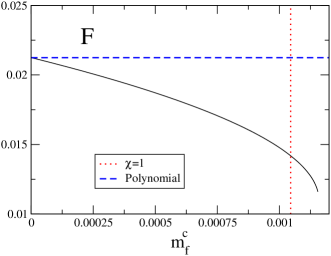
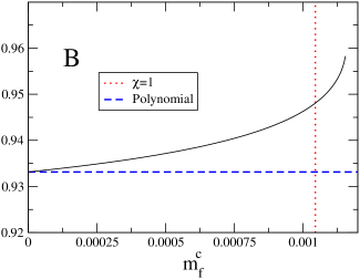
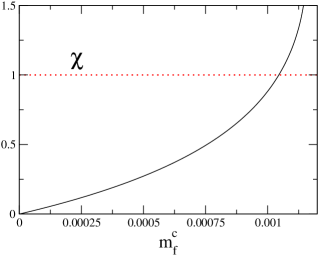
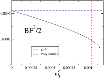
Appendix F Hyperscaling analyses
F.1 Effective mass anomalous dimension
In Sec. V.2, we investigated the effective mass anomalous dimension . In Table 32, we show the numerical results of for . For , the Large Volume Data Set explained in Sec. III.1 is used to obtain the . For , the available data are limited to the updated ensemble, for which the is computed. In Tables 33 and 34, we show the for with and , respectively. The spectrum data are summarized in Appendix G, from which the results obtained at the largest volumes are used to obtain the . The shown in this appendix are shown in Fig. 33.
| fit range | ||||||||
|---|---|---|---|---|---|---|---|---|
| 0.012-0.02 | 0.706(16) | 0.65 | 1.132(104) | 0.0007 | 0.987(40) | 1.25 | 1.003(79) | 0.78 |
| 0.015-0.03 | 0.676(7) | 0.69 | 0.856(49) | 2.74 | 0.989(16) | 0.60 | 0.783(32) | 1.23 |
| 0.02-0.04 | 0.654(6) | 1.66 | 0.841(50) | 2.25 | 1.004(15) | 0.019 | 0.899(42) | 9.63 |
| 0.03-0.05 | 0.647(8) | 0.25 | 0.947(89) | 0.069 | 1.031(21) | 3.15 | - | - |
| 0.03-0.06 | - | - | - | - | - | - | 0.904(43) | 9.39 |
| 0.04-0.06 | 0.625(6) | 3.64 | 0.904(55) | 0.012 | 0.994(19) | 6.62 | - | - |
| 0.04-0.08 | - | - | - | - | - | - | 0.780(36) | 1.05 |
| 0.05-0.07 | 0.599(14) | 0.62 | 1.024(247) | 0.070 | 0.962(43) | 7.39 | - | - |
| 0.06-0.08 | 0.598(8) | 0.54 | 0.971(84) | 0.13 | 1.009(31) | 3.55 | - | - |
| 0.07-0.10 | 0.563(10) | 0.45 | 0.622(96) | 0.73 | 0.888(32) | 0.31 | - | - |
| fit range | ||||||||
|---|---|---|---|---|---|---|---|---|
| 0.04-0.06 | 0.402(12) | 0.007 | 0.443(27) | 0.03 | 0.449(25) | 1.0 | 0.427(31) | 0.009 |
| 0.05-0.08 | 0.389(5) | 0.60 | 0.400(11) | 2.0 | 0.443(14) | 0.9 | 0.400(0.016) | 0.3 |
| 0.06-0.1 | 0.396(4) | 3.0 | 0.416(9) | 4.9 | 0.473(12) | 6.5 | 0.406(14) | 0.6 |
| 0.08-0.12 | 0.406(4) | 0.004 | 0.439(12) | 0.7 | 0.520(14) | 0.2 | 0.437(20) | 0.1 |
| 0.1-0.16 | 0.410(3) | 0.2 | 0.456(6) | 2.4 | 0.568(10) | 3.9 | 0.470(13) | 0.4 |
| 0.12-0.2 | 0.399(3) | 8.8 | 0.473(8) | 0.05 | 0.563(25) | 4.7 | 0.487(13) | 0.05 |
| 0.16-0.24 | 0.391(4) | 1.7 | 0.476(10) | 0.6 | 0.543(13) | 0.4 | 0.483(23) | 1.2 |
| 0.2-0.3 | 0.411(2) | 0.03 | 0.513(8) | 0.1 | 0.635(7) | 0.06 | 0.477(11) | 1.1 |
| fit range | ||||||||
|---|---|---|---|---|---|---|---|---|
| 0.035-0.05 | 0.401(14) | 0.07 | 0.381(31) | 0.2 | 0.386(29) | 1.0 | 0.392(32) | 0.3 |
| 0.04-0.06 | 0.413(10) | 0.8 | 0.399(18) | 0.08 | 0.422(18) | 0.01 | 0.406(23) | 0.0004 |
| 0.05-0.08 | 0.435(8) | 0.6 | 0.445(20) | 1.1 | 0.538(18) | 6.3 | 0.431(20) | 0.3 |
| 0.06-0.1 | 0.449(4) | 0.4 | 0.456(14) | 0.09 | 0.550(12) | 1.2 | 0.471(15) | 0.8 |
| 0.08-0.12 | 0.446(7) | 0.9 | 0.474(21) | 0.6 | 0.500(14) | 0.5 | 0.445(17) | 3.2 |
| 0.1-0.16 | 0.442(3) | 0.03 | 0.500(13) | 0.0008 | 0.565(11) | 7.6 | 0.4675(97) | 5.7 |
| 0.12-0.2 | 0.443(2) | 0.01 | 0.523(9) | 2.2 | 0.604(8) | 0.2 | 0.4585(64) | 7.2 |
| 0.16-0.3 | 0.451(1) | 2.8 | 0.559(5) | 0.4 | 0.610(4) | 0.0007 | 0.4643(63) | 24.4 |
F.2 FSHS analyses for with various cuts
In Table 35, we tabulate the mass anomalous dimension obtained by adopting the linear FSHS ansatz (43) for various data selection schemes: and FSHS-Large Volume Data Set. We investigate which data set achieves linear dependence on . We focus on the for and for which the fit works in most cases. The scheme and give a statistically equivalent , and hence, the selection excludes enough the non-linearity at small X. Then, the results by the FSHS-Large Volume data set is consistent to those in the data set with , and therefore, it would also be free from the non-linearity.
For all selection schemes, the linear FSHS fit for fails. Therefore, the non-linearlity typically appearing at small would not be the reason for the deviation from the linear ansatz (43), in the case of . A possible origin of the deviation is chiral dynamics as discussed in Sec. V.4.
| Data Set () | dof | ||||||
|---|---|---|---|---|---|---|---|
| FSHS-Large Vol. Data |
F.3 Global parameter search in Renormalization group (RG)-motivated FSHS
In Sec. V.3.4, we have investigated the spectrum data by using the RG-motivated FSHS ansatz, where we have two exponents in the fit function (50). This fit provided the results shown in the last line in Table 15. It is important to confirm that the exponents have been obtained from the global minimum in the parameter space.
In Fig. 56, we show as a function of (left panel) and the corresponding (right panel). is well determined without any instabilities, and the has a clear minimum around , which is consistent to what we have found by treating as a fit parameter in Sec. V.3.4: . For larger , the fit ansatz (50) reduces into the naive one (43), which is shown to give a large (Sec. V.3.2). Consistently, we observe a larger with increasing in the right panel of Fig. 56.
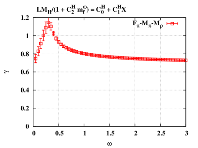
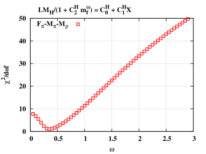
Appendix G
We have simulated QCD at and . In this Appendix we show a brief summary of results for the spectrum of QCD.
We have accumulated additional statistics for and since the previous result shown in Ref. Aoki et al. (2012b), and also have new data at a larger volume of . The simulation parameters and results for the hadron spectrum at and are summarized in Tables 36, 37 38, and 39 (For , see Ref. Aoki et al. (2012b)).
The fermion mass dependence of the basic hadron spectra of , , , and is shown in Fig. 57, Fig. 58, Fig. 59, and Fig. 60. Using those spectrum quantities, the ratios of , , and to are shown in Fig. 61, Fig. 62, and Fig. 63, where all the ratios become constant in the smaller region for both and , which is consistent with being in the conformal phase in .
The mild fermion mass dependence at larger could be considered as a correction to the hyperscaling due to the large fermion mass effect as shown in the previous paper Aoki et al. (2012b). In fact, the result of the effective analysis shown in Fig. 33 indicates universal hyperscaling in the small mass region, thus both the results of the effective and ratio analyses are consistent with being in the conformal phase, which is clearly different from the result obtained in QCD.
The ratios of , , and are shown in Figs. 64, 65, and 66. While those quantities have larger errors, each ratio becomes a constant in the small mass region. From the value of the constant for each ratio, we may further read and in the smaller fermion mass region. According to the “Mended Symmetry”, our result in suggests the chiral restoration through the “vector manifestation”, where and . (For details, see Sec. VIII.) We also note that those mass ratios are different to those in QCD, and hadron masses are more degenerate in than .
| 36 | 48 | 0.040 | 4000 | 250 | 160 | 4 |
| 36 | 48 | 0.050 | 8000 | 250 | 320 | 4 |
| 36 | 48 | 0.060 | 8000 | 250 | 320 | 4 |
| 36 | 48 | 0.080 | 4000 | 250 | 160 | 4 |
| 30 | 40 | 0.040 | 1000 | 250 | 100 | 4 |
| 30 | 40 | 0.050 | 4000 | 250 | 160 | 4 |
| 30 | 40 | 0.060 | 4000 | 250 | 160 | 4 |
| 30 | 40 | 0.080 | 4000 | 250 | 320 | 4 |
| 30 | 40 | 0.100 | 4000 | 250 | 160 | 4 |
| 30 | 40 | 0.120 | 1000 | 250 | 40 | 4 |
| 30 | 40 | 0.160 | 1000 | 250 | 40 | 4 |
| 30 | 40 | 0.200 | 1000 | 250 | 40 | 4 |
| 24 | 32 | 0.040 | 2000 | 250 | 80 | 4 |
| 24 | 32 | 0.050 | 8000 | 250 | 160 | 4 |
| 24 | 32 | 0.060 | 8000 | 250 | 160 | 4 |
| 24 | 32 | 0.080 | 8000 | 250 | 160 | 4 |
| 24 | 32 | 0.100 | 8000 | 250 | 160 | 4 |
| 24 | 32 | 0.120 | 2000 | 250 | 80 | 4 |
| 24 | 32 | 0.160 | 1000 | 250 | 100 | 4 |
| 24 | 32 | 0.200 | 1000 | 250 | 100 | 4 |
| 36 | 48 | 0.035 | 4000 | 750 | 200 | 4 |
| 36 | 48 | 0.040 | 2600 | 650 | 100 | 4 |
| 36 | 48 | 0.050 | 2000 | 500 | 100 | 4 |
| 36 | 48 | 0.060 | 2000 | 500 | 100 | 4 |
| 30 | 40 | 0.035 | 2000 | 250 | 80 | 4 |
| 30 | 40 | 0.040 | 3000 | 750 | 100 | 4 |
| 30 | 40 | 0.050 | 1700 | 425 | 100 | 4 |
| 30 | 40 | 0.060 | 2000 | 500 | 100 | 4 |
| 30 | 40 | 0.080 | 1000 | 250 | 100 | 4 |
| 30 | 40 | 0.100 | 500 | 125 | 20 | 4 |
| 30 | 40 | 0.120 | 500 | 125 | 20 | 4 |
| 30 | 40 | 0.160 | 500 | 125 | 20 | 4 |
| 30 | 40 | 0.200 | 500 | 125 | 20 | 4 |
| 30 | 40 | 0.200 | 400 | 100 | 20 | 4 |
| 24 | 32 | 0.040 | 2000 | 250 | 80 | 4 |
| 24 | 32 | 0.050 | 2000 | 250 | 80 | 4 |
| 24 | 32 | 0.060 | 2000 | 250 | 80 | 4 |
| 24 | 32 | 0.080 | 1000 | 125 | 40 | 4 |
| 24 | 32 | 0.100 | 1000 | 125 | 40 | 4 |
| 24 | 32 | 0.120 | 1000 | 125 | 40 | 4 |
| 24 | 32 | 0.160 | 1000 | 125 | 40 | 4 |
| 24 | 32 | 0.200 | 1000 | 125 | 40 | 4 |
| 24 | 32 | 0.300 | 1000 | 125 | 40 | 4 |
| 36 | 48 | 0.04 | 0.2718(7) | 0.3247(20) | 0.4964(28) | 0.3820(21) | 0.4197(44) | 0.4258(61) | 0.05438(27) |
|---|---|---|---|---|---|---|---|---|---|
| 36 | 48 | 0.05 | 0.3186(4) | 0.3794(9) | 0.5802(15) | 0.4469(25) | 0.4948(41) | 0.5012(48) | 0.06374(17) |
| 36 | 48 | 0.06 | 0.3629(3) | 0.4303(9) | 0.6595(22) | 0.5032(36) | 0.5552(22) | 0.5624(27) | 0.07210(16) |
| 36 | 48 | 0.08 | 0.4467(3) | 0.5301(9) | 0.8115(23) | 0.6237(35) | 0.6815(24) | 0.6890(33) | 0.08819(16) |
| 30 | 40 | 0.04 | 0.2753(16) | 0.3295(49) | 0.5148(55) | 0.3813(88) | 0.423(12) | 0.432(15) | 0.05477(63) |
| 30 | 40 | 0.05 | 0.3186(7) | 0.3798(14) | 0.5825(20) | 0.4396(33) | 0.4877(49) | 0.4926(46) | 0.06325(27) |
| 30 | 40 | 0.06 | 0.3638(5) | 0.4325(13) | 0.6611(18) | 0.4977(36) | 0.5546(39) | 0.5647(39) | 0.07208(19) |
| 30 | 40 | 0.08 | 0.4465(4) | 0.5292(12) | 0.8091(16) | 0.6223(33) | 0.6778(24) | 0.6864(27) | 0.08809(17) |
| 30 | 40 | 0.1 | 0.5235(3) | 0.6182(7) | 0.9489(18) | 0.7283(41) | 0.7926(28) | 0.7878(48) | 0.10203(18) |
| 30 | 40 | 0.12 | 0.5960(4) | 0.7027(11) | 1.0762(28) | 0.8293(60) | 0.8928(45) | 0.8762(68) | 0.11514(19) |
| 30 | 40 | 0.16 | 0.7306(3) | 0.8541(7) | 1.3067(26) | 1.0171(90) | 1.0855(76) | 1.053(12) | 0.13790(13) |
| 30 | 40 | 0.2 | 0.8580(3) | 0.9940(11) | 1.5176(23) | 1.192(13) | 1.261(12) | 1.235(25) | 0.15938(11) |
| 24 | 32 | 0.04 | 0.3047(28) | 0.3520(57) | 0.5789(58) | 0.3374(31) | 0.3969(60) | 0.4076(76) | 0.05128(48) |
| 24 | 32 | 0.05 | 0.3259(11) | 0.3934(24) | 0.6112(34) | 0.4162(50) | 0.4792(84) | 0.484(12) | 0.06321(34) |
| 24 | 32 | 0.06 | 0.3662(9) | 0.4366(19) | 0.6761(24) | 0.5005(54) | 0.5640(46) | 0.5648(39) | 0.07218(30) |
| 24 | 32 | 0.08 | 0.4474(5) | 0.5305(14) | 0.8165(23) | 0.6129(47) | 0.6782(26) | 0.6890(31) | 0.08800(21) |
| 24 | 32 | 0.1 | 0.5240(4) | 0.6193(12) | 0.9501(20) | 0.7250(44) | 0.7895(22) | 0.7950(33) | 0.10220(18) |
| 24 | 32 | 0.12 | 0.5957(5) | 0.7034(15) | 1.0754(28) | 0.8471(83) | 0.8893(38) | 0.8920(58) | 0.11483(17) |
| 24 | 32 | 0.16 | 0.7313(5) | 0.8539(15) | 1.3015(77) | 1.0172(87) | 1.0786(68) | 1.054(12) | 0.13835(25) |
| 24 | 32 | 0.2 | 0.8568(3) | 0.9934(15) | 1.5212(36) | 1.191(20) | 1.264(18) | 1.276(42) | 0.15878(19) |
| 24 | 32 | 0.3 | 1.1435(2) | 1.2996(13) | 1.9971(28) | 1.497(24) | 1.589(26) | 1.488(50) | 0.20425(14) |
| 36 | 48 | 0.035 | 0.2727(7) | 0.3326(26) | 0.5062(28) | 0.3913(28) | 0.4364(52) | 0.4408(64) | 0.05734(24) |
|---|---|---|---|---|---|---|---|---|---|
| 36 | 48 | 0.04 | 0.2997(6) | 0.3677(12) | 0.5589(20) | 0.4316(31) | 0.4707(56) | 0.4893(40) | 0.06345(21) |
| 36 | 48 | 0.05 | 0.3516(4) | 0.4317(12) | 0.6550(22) | 0.5028(28) | 0.5658(26) | 0.5752(28) | 0.07427(26) |
| 36 | 40 | 0.06 | 0.3997(3) | 0.4914(10) | 0.7457(22) | 0.5737(34) | 0.6455(28) | 0.6546(32) | 0.08439(14) |
| 30 | 40 | 0.035 | 0.2770(11) | 0.3369(38) | 0.5206(40) | 0.3548(4) | 0.4314(45) | 0.4405(45) | 0.05744(36) |
| 30 | 40 | 0.04 | 0.30146(7) | 0.3685(17) | 0.5634(24) | 0.4363(33) | 0.4820(36) | 0.4971(32) | 0.06361(25) |
| 30 | 40 | 0.05 | 0.3524(6) | 0.4334(17) | 0.6580(27) | 0.4963(55) | 0.5571(53) | 0.5650(58) | 0.07407(21) |
| 30 | 40 | 0.06 | 0.3985(5) | 0.4872(11) | 0.7420(25) | 0.5618(43) | 0.6401(29) | 0.6458(35) | 0.08331(21) |
| 30 | 40 | 0.08 | 0.4879(7) | 0.5980(22) | 0.9101(30) | 0.6977(56) | 0.7788(46) | 0.7820(54) | 0.10135(21) |
| 30 | 40 | 0.1 | 0.5686(4) | 0.6980(2) | 1.0559(19) | 0.8103(97) | 0.927(14) | 0.934(16) | 0.11739(24) |
| 30 | 40 | 0.12 | 0.6453(4) | 0.7881(14) | 1.2017(17) | 0.926(10) | 1.0120(49) | 1.006(10) | 0.13278(20) |
| 30 | 40 | 0.16 | 0.7878(3) | 0.9547(13) | 1.4571(19) | 1.123(11) | 1.2242(79) | 1.192(23) | 0.15897(17) |
| 30 | 40 | 0.2 | 0.9195(3) | 1.1028(12) | 1.6739(69) | 1.318(14) | 1.408(10) | 1.319(21) | 0.18261(15) |
| 30 | 40 | 0.3 | 1.2155(2) | 1.4296(8) | 2.155(17) | 1.726(15) | 1.831(22) | 1.67(19) | 0.23492(13) |
| 24 | 32 | 0.04 | 0.3043(19) | 0.3702(61) | 0.5961(96) | 0.4260(65) | 0.4764(49) | 0.4976(64) | 0.06161(64) |
| 24 | 32 | 0.05 | 0.3533(10) | 0.4372(31) | 0.6715(32) | 0.4803(47) | 0.5623(40) | 0.5649(45) | 0.07359(49) |
| 24 | 32 | 0.06 | 0.3988(8) | 0.4941(16) | 0.7502(24) | 0.5576(45) | 0.6340(40) | 0.6460(45) | 0.08389(24) |
| 24 | 32 | 0.08 | 0.4863(7) | 0.5967(18) | 0.9047(31) | 0.7053(81) | 0.7716(35) | 0.7878(48) | 0.10082(30) |
| 24 | 32 | 0.1 | 0.5685(8) | 0.6968(15) | 1.0586(36) | 0.8227(82) | 0.9084(60) | 0.9126(75) | 0.11756(27) |
| 24 | 32 | 0.12 | 0.6447(4) | 0.7855(17) | 1.2006(30) | 0.9179(66) | 1.0131(65) | 1.010(13) | 0.13227(31) |
| 24 | 32 | 0.16 | 0.7883(4) | 0.9539(23) | 1.4592(25) | 1.128(14) | 1.222(14) | 1.1574(15) | 0.15885(22) |
| 24 | 32 | 0.2 | 0.9198(3) | 1.1056(25) | 1.6865(27) | 1.313(20) | 1.430(49) | 1.5(1.0) | 0.18265(22) |
| 24 | 32 | 0.3 | 1.2158(3) | 1.4310(11) | 2.167(15) | 1.773(60) | 1.824(25) | 1.707(66) | 0.23513(15) |
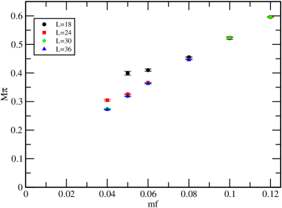
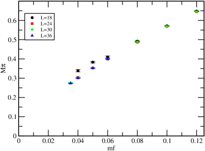
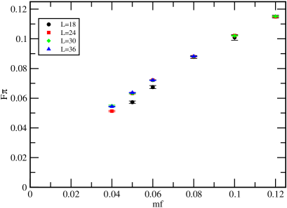
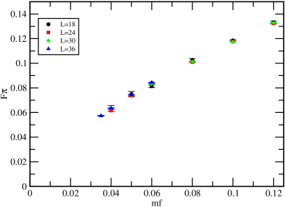
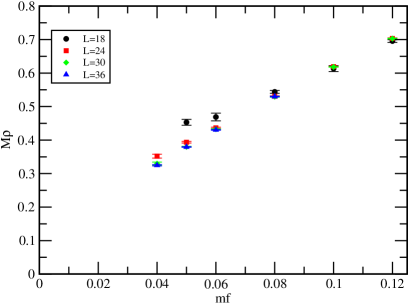
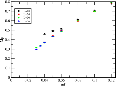
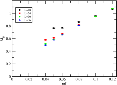
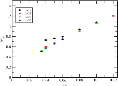
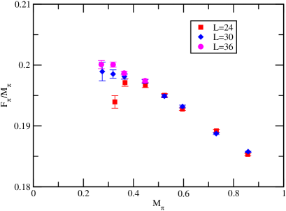
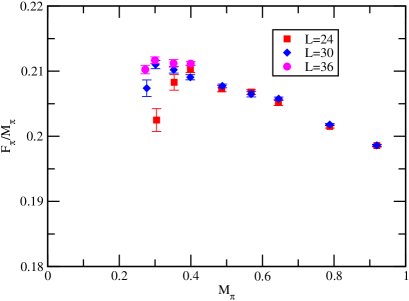
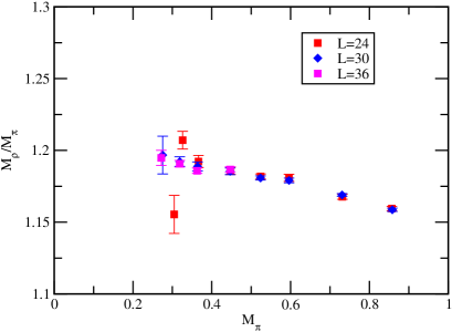
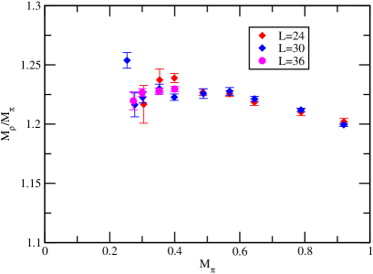
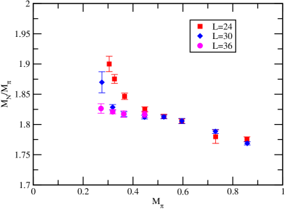
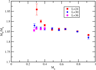
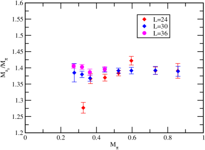
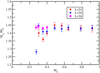
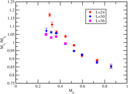
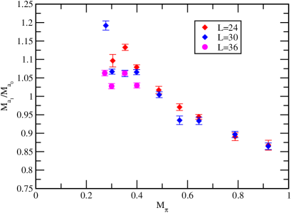
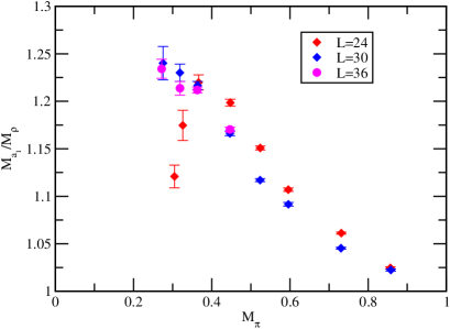
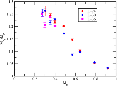
References
- Yamawaki et al. (1986) K. Yamawaki, M. Bando, and K.-i. Matumoto, Phys. Rev. Lett. 56, 1335 (1986).
- Bando et al. (1986) M. Bando, K.-i. Matumoto, and K. Yamawaki, Phys. Lett. B178, 308 (1986).
- Holdom (1985) B. Holdom, Phys. Lett. B150, 301 (1985).
- Akiba and Yanagida (1986) T. Akiba and T. Yanagida, Phys. Lett. B169, 432 (1986).
- Appelquist et al. (1986) T. W. Appelquist, D. Karabali, and L. C. R. Wijewardhana, Phys. Rev. Lett. 57, 957 (1986).
- Matsuzaki and Yamawaki (2012a) S. Matsuzaki and K. Yamawaki, Phys. Rev. D 86, 115004 (2012a).
- Matsuzaki and Yamawaki (2013) S. Matsuzaki and K. Yamawaki, Phys. Lett. B719, 378 (2013).
- Yamawaki (2017) K. Yamawaki, Int. J. Mod. Phys. E26, 1740032 (2017), arXiv:1609.03715 [hep-ph] .
- Appelquist et al. (1996) T. Appelquist, J. Terning, and L. C. R. Wijewardhana, Phys. Rev. Lett. 77, 1214 (1996).
- Miransky and Yamawaki (1997) V. A. Miransky and K. Yamawaki, Phys. Rev. D 55, 5051 (1997).
- Caswell (1974) W. E. Caswell, Phys. Rev. Lett. 33, 244 (1974).
- Banks and Zaks (1982) T. Banks and A. Zaks, Nucl. Phys. B196, 189 (1982).
- Aoki et al. (2012a) Y. Aoki, T. Aoyama, M. Kurachi, T. Maskawa, K.-i. Nagai, H. Ohki, A. Shibata, K. Yamawaki, and T. Yamazaki (LatKMI Collaboration), Phys. Rev. D 85, 074502 (2012a).
- Matsuzaki and Yamawaki (2015) S. Matsuzaki and K. Yamawaki, JHEP 12, 053 (2015).
- Aoki et al. (2013a) Y. Aoki, T. Aoyama, M. Kurachi, T. Maskawa, K.-i. Nagai, H. Ohki, A. Shibata, K. Yamawaki, and T. Yamazaki (LatKMI Collaboration), Phys. Rev. D 87, 094511 (2013a).
- Kuti (2014) J. Kuti, PoS LATTICE2013, 004 (2014).
- DeGrand (2016) T. DeGrand, Rev. Mod. Phys. 88, 015001 (2016).
- Aoki (2014) Y. Aoki, Plenary talk presented at the 32nd International Symposium on Lattice Field Theory (Lattice 2014) (2014).
- Hasenfratz (2015) A. Hasenfratz, Plenary talk presented at 33rd International Symposium on Lattice Field Theory (Lattice 2015) (2015).
- Iwasaki et al. (1992) Y. Iwasaki, K. Kanaya, S. Sakai, and T. Yoshie, Phys. Rev. Lett. 69, 21 (1992).
- Aoki et al. (2012b) Y. Aoki, T. Aoyama, M. Kurachi, T. Maskawa, K.-i. Nagai, H. Ohki, A. Shibata, K. Yamawaki, and T. Yamazaki (LatKMI Collaboration), Phys. Rev. D 86, 054506 (2012b).
- Fodor et al. (2011) Z. Fodor, K. Holland, J. Kuti, D. Nogradi, C. Schroeder, K. Holland, J. Kuti, D. Nogradi, and C. Schroeder, Phys. Lett. B703, 348 (2011).
- Hayakawa et al. (2011) M. Hayakawa, K. I. Ishikawa, Y. Osaki, S. Takeda, S. Uno, and N. Yamada, Phys. Rev. D 83, 074509 (2011).
- Dimopoulos (1980) S. Dimopoulos, Nucl. Phys. B168, 69 (1980).
- Farhi and Susskind (1981) E. Farhi and L. Susskind, Phys. Rept. 74, 277 (1981).
- Dimopoulos and Susskind (1979) S. Dimopoulos and L. Susskind, Nucl. Phys. B155, 237 (1979).
- Eichten and Lane (1980) E. Eichten and K. D. Lane, Phys. Lett. B90, 125 (1980).
- Aoki et al. (2014) Y. Aoki, T. Aoyama, M. Kurachi, T. Maskawa, K. Miura, K.-i. Nagai, H. Ohki, E. Rinaldi, A. Shibata, K. Yamawaki, and T. Yamazaki (LatKMI Collaboration), PoS LATTICE2013, 070 (2014).
- Aoki et al. (2014) Y. Aoki, T. Aoyama, M. Kurachi, T. Maskawa, K. Miura, K.-i. Nagai, H. Ohki, E. Rinaldi, A. Shibata, K. Yamawaki, and T. Yamazaki (LatKMI Collaboration), Phys. Rev. D 89, 111502 (2014).
- Appelquist et al. (2008) T. Appelquist, G. T. Fleming, and E. T. Neil, Phys. Rev. Lett. 100, 171607 (2008).
- Hasenfratz et al. (2015) A. Hasenfratz, D. Schaich, and A. Veernala, JHEP 06, 143 (2015).
- Ishikawa et al. (2013) K. I. Ishikawa, Y. Iwasaki, Y. Nakayama, and T. Yoshie, Phys. Rev. D87, 071503 (2013).
- Appelquist et al. (2014a) T. Appelquist, R. C. Brower, G. T. Fleming, J. Kiskis, M. F. Lin, E. T. Neil, J. C. Osborn, C. Rebbi, E. Rinaldi, D. Schaich, C. Schroeder, S. Syritsyn, G. Voronov, P. Vranas, E. Weinberg, and O. Witzel (Lattice Strong Dynamics (LSD) Collaboration), Phys. Rev. D 90, 114502 (2014a).
- Appelquist et al. (2016) T. Appelquist, R. C. Brower, G. T. Fleming, A. Hasenfratz, X. Y. Jin, J. Kiskis, E. T. Neil, J. C. Osborn, C. Rebbi, E. Rinaldi, D. Schaich, P. Vranas, E. Weinberg, and O. Witzel (Lattice Strong Dynamics (LSD) Collaboration), Phys. Rev. D 93, 114514 (2016).
- Aoki et al. (2013b) Y. Aoki, T. Aoyama, M. Kurachi, T. Maskawa, K.-i. Nagai, H. Ohki, E. Rinaldi, A. Shibata, K. Yamawaki, and T. Yamazaki (LatKMI Collaboration), Phys. Rev. Lett. 111, 162001 (2013b).
- Fodor et al. (2014) Z. Fodor, K. Holland, J. Kuti, D. Nogradi, and C. H. Wong, PoS LATTICE2013, 062 (2014).
- Kunihiro et al. (2004) T. Kunihiro, S. Muroya, A. Nakamura, C. Nonaka, M. Sekiguchi, and H. Wada (SCALAR Collaboration), Phys. Rev. D 70, 034504 (2004).
- Aoki et al. (2015a) Y. Aoki, T. Aoyama, E. Bennett, M. Kurachi, T. Maskawa, K. Miura, K.-i. Nagai, H. Ohki, E. Rinaldi, A. Shibata, K. Yamawaki, and T. Yamazaki (LatKMI Collaboration), PoS LATTICE2014, 256 (2015a).
- Aoki et al. (2015b) Y. Aoki, T. Aoyama, E. Bennett, M. Kurachi, T. Maskawa, K. Miura, K.-i. Nagai, H. Ohki, E. Rinaldi, A. Shibata, K. Yamawaki, and T. Yamazaki (LatKMI Collaboration), (2015b), arXiv:1510.07373 [hep-lat] .
- Aoki et al. (2016a) Y. Aoki, T. Aoyama, E. Bennett, M. Kurachi, T. Maskawa, K. Miura, K.-i. Nagai, H. Ohki, E. Rinaldi, A. Shibata, K. Yamawaki, and T. Yamazaki (LatKMI Collaboration), PoS LATTICE2015, 213 (2016a).
- Aoki et al. (2016b) Y. Aoki, T. Aoyama, E. Bennett, M. Kurachi, T. Maskawa, K. Miura, K.-i. Nagai, H. Ohki, E. Rinaldi, A. Shibata, K. Yamawaki, and T. Yamazaki (LatKMI Collaboration), PoS LATTICE2015, 215 (2016b).
- Cheng et al. (2014) A. Cheng, A. Hasenfratz, Y. Liu, G. Petropoulos, and D. Schaich, Phys. Rev. D 90, 014509 (2014).
- Matsuzaki and Yamawaki (2014) S. Matsuzaki and K. Yamawaki, Phys. Rev. Lett. 113, 082002 (2014).
- Follana et al. (2007) E. Follana, Q. Mason, C. Davies, K. Hornbostel, G. P. Lepage, J. Shigemitsu, H. Trottier, and K. Wong, Phys. Rev. D 75, 054502 (2007).
- Bazavov et al. (2010) A. Bazavov, C. Bernard, C. DeTar, W. Freeman, S. Gottlieb, U. M. Heller, J. E. Hetrick, J. Laiho, L. Levkova, M. Oktay, J. Osborn, R. L. Sugar, D. Toussaint, and R. S. Van de Water (MILC Collaboration), Phys. Rev. D 82, 074501 (2010).
- Bazavov et al. (2012) A. Bazavov, T. Bhattacharya, M. Cheng, C. DeTar, H.-T. Ding, S. Gottlieb, R. Gupta, P. Hegde, U. M. Heller, F. Karsch, E. Laermann, L. Levkova, S. Mukherjee, P. Petreczky, C. Schmidt, R. A. Soltz, W. Soeldner, R. Sugar, D. Toussaint, W. Unger, and P. Vranas (HotQCD Collaboration), Phys. Rev. D 85, 054503 (2012).
- Peskin and Takeuchi (1990) M. E. Peskin and T. Takeuchi, Phys. Rev. Lett. 65, 964 (1990).
- Aoki et al. (2016c) Y. Aoki, T. Aoyama, E. Bennett, M. Kurachi, T. Maskawa, K. Miura, K.-i. Nagai, H. Ohki, E. Rinaldi, A. Shibata, K. Yamawaki, and T. Yamazaki (LatKMI Collaboration), PoS LATTICE2015, 245 (2016c).
- Duane et al. (1987) S. Duane, A. D. Kennedy, B. J. Pendleton, and D. Roweth, Phys. Lett. B195, 216 (1987).
- Hasenbusch (2001) M. Hasenbusch, Phys. Lett. B519, 177 (2001).
- (51) See http://www.physics.utah.edu/~detar/milc/milc_qcd.html .
- Gupta (1997) R. Gupta (1997) hep-lat/9807028 .
- Kilcup and Sharpe (1987) G. W. Kilcup and S. R. Sharpe, Nucl. Phys. B283, 493 (1987).
- Blum et al. (2003) T. Blum et al. (RBC), Phys. Rev. D68, 114506 (2003), hep-lat/0110075 .
- Umeda (2007) T. Umeda, Phys. Rev. D75, 094502 (2007), arXiv:hep-lat/0701005 [hep-lat] .
- Golterman and Smit (1984) M. F. Golterman and J. Smit, Nucl.Phys. B245, 61 (1984).
- Golterman (1986) M. F. L. Golterman, Nucl. Phys. B273, 663 (1986).
- Ishizuka et al. (1994) N. Ishizuka, M. Fukugita, H. Mino, M. Okawa, and A. Ukawa, Nucl. Phys. B411, 875 (1994).
- Golterman and Smit (1985) M. F. L. Golterman and J. Smit, Nucl. Phys. B255, 328 (1985).
- Gasser and Leutwyler (1988) J. Gasser and H. Leutwyler, Nucl. Phys. B307, 763 (1988).
- Luscher (1986) M. Luscher, Commun. Math. Phys. 104, 177 (1986).
- Aubin et al. (2004) C. Aubin, C. Bernard, C. DeTar, J. Osborn, S. Gottlieb, E. B. Gregory, D. Toussaint, U. M. Heller, J. E. Hetrick, and R. Sugar (MILC Collaboration), Phys. Rev. D 70, 114501 (2004).
- Fodor et al. (2009) Z. Fodor, K. Holland, J. Kuti, D. Nogradi, and C. Schroeder, Phys. Lett. B681, 353 (2009).
- Soldate and Sundrum (1990) M. Soldate and R. Sundrum, Nucl. Phys. B340, 1 (1990).
- Chivukula et al. (1993) R. S. Chivukula, M. J. Dugan, and M. Golden, Phys. Rev. D 47, 2930 (1993).
- Harada and Yamawaki (2003) M. Harada and K. Yamawaki, Phys. Rept. 381, 1 (2003).
- Gasser and Leutwyler (1984) J. Gasser and H. Leutwyler, Ann. Phys. 158, 142 (1984).
- Weinberg (1967) S. Weinberg, Phys. Rev. Lett. 18, 507 (1967).
- Gilman and Harari (1968) F. J. Gilman and H. Harari, Phys. Rev. 165, 1803 (1968).
- Weinberg (1969) S. Weinberg, Phys. Rev. 177, 2604 (1969).
- Weinberg (1990) S. Weinberg, Phys. Rev. Lett. 65, 1177 (1990).
- Maskawa and Yamawaki (1976) T. Maskawa and K. Yamawaki, Prog. Theor. Phys. 56, 270 (1976).
- Yamawaki (1998) K. Yamawaki, in QCD, light cone physics and hadron phenomenology. Proceedings, 10th Nuclear Summer School and Symposium, NuSS’97, Seoul, Korea, June 23-28, 1997 (1998) pp. 116–199, arXiv:hep-th/9802037 [hep-th] .
- Ida (1974) M. Ida, Prog. Theor. Phys. 51, 1521 (1974), [Erratum: Prog. Theor. Phys.52,1978(1974)].
- Del Debbio and Zwicky (2010) L. Del Debbio and R. Zwicky, Phys. Rev. D 82, 014502 (2010).
- Albanese et al. (1987) M. Albanese, F. Costantini, G. Fiorentini, F. Flore, M. Lombardo, R. Tripiccione, P. Bacilieri, L. Fonti, P. Giacomelli, E. Remiddi, M. Bernaschi, N. Cabibbo, E. Marinari, G. Parisi, G. Salina, S. Cabasino, F. Marzano, P. Paolucci, S. Petrarca, F. Rapuano, P. Marchesini, and R. Rusack (APE Collaboration), Phys. Lett. B 192, 163 (1987).
- Hasenfratz and Knechtli (2001) A. Hasenfratz and F. Knechtli, Phys. Rev. D 64, 034504 (2001).
- Della Morte et al. (2004) M. Della Morte, S. Durr, J. Heitger, H. Molke, J. Rolf, A. Shindler, and R. Sommer (ALPHA Collaboration), Phys. Lett. B581, 93 (2004), [Erratum: Phys. Lett.B612,313(2005)].
- Della Morte et al. (2005) M. Della Morte, A. Shindler, and R. Sommer, JHEP 08, 051 (2005).
- Hasenfratz (2010) A. Hasenfratz, Phys. Rev. D 82, 014506 (2010).
- Brower et al. (2016) R. C. Brower, A. Hasenfratz, C. Rebbi, E. Weinberg, and O. Witzel, Phys. Rev. D 93, 075028 (2016).
- Venkataraman and Kilcup (1997) L. Venkataraman and G. Kilcup, Submitted to: Phys. Rev. D (1997).
- Gregory et al. (2008) E. B. Gregory, A. C. Irving, C. M. Richards, and C. McNeile, Phys. Rev. D 77, 065019 (2008).
- McNeile et al. (2013) C. McNeile, A. Bazavov, C. T. H. Davies, R. J. Dowdall, K. Hornbostel, G. P. Lepage, and H. D. Trottier, Phys. Rev. D 87, 034503 (2013).
- Jin and Mawhinney (2011) X.-Y. Jin and R. D. Mawhinney, PoS LATTICE2011, 066 (2011).
- Kosower (1984) D. A. Kosower, Phys. Lett. B144, 215 (1984).
- Peskin (1980) M. E. Peskin, Nucl. Phys. B175, 197 (1980).
- Bando et al. (1988) M. Bando, T. Kugo, and K. Yamawaki, Phys. Rept. 164, 217 (1988).
- Aad et al. (2015) G. Aad et al. (ATLAS), Eur. Phys. J. C75, 476 (2015), [Erratum: Eur. Phys. J.C76,no.3,152(2016)], arXiv:1506.05669 [hep-ex] .
- Khachatryan et al. (2015) V. Khachatryan et al. (CMS), Phys. Rev. D92, 012004 (2015), arXiv:1411.3441 [hep-ex] .
- Matsuzaki and Yamawaki (2012b) S. Matsuzaki and K. Yamawaki, Phys. Rev. D 86, 035025 (2012b).
- Appelquist et al. (2014b) T. Appelquist, E. Berkowitz, R. C. Brower, M. I. Buchoff, G. T. Fleming, J. Kiskis, M. F. Lin, E. T. Neil, J. C. Osborn, C. Rebbi, E. Rinaldi, D. Schaich, C. Schroeder, S. Syritsyn, G. Voronov, P. Vranas, E. Weinberg, O. Witzel, and G. D. Kribs (Lattice Strong Dynamics (LSD) Collaboration), Phys. Rev. D 89, 094508 (2014b).
- Akerib et al. (2014) D. S. Akerib et al. (LUX Collaboration), Phys. Rev. Lett. 112, 091303 (2014).
- Akerib et al. (2016) D. S. Akerib et al., (2016), arXiv:1608.07648 [astro-ph.CO] .
- Tan et al. (2016) A. Tan et al. (PandaX-II Collaboration), Phys. Rev. Lett. 117, 121303 (2016).
- Fodor et al. (2016) Z. Fodor, K. Holland, J. Kuti, S. Mondal, D. Nogradi, and C. H. Wong, Phys. Rev. D 94, 014503 (2016).
- Holdom and Terning (1990) B. Holdom and J. Terning, Phys. Lett. B247, 88 (1990).
- Golden and Randall (1991) M. Golden and L. Randall, Nucl. Phys. B361, 3 (1991).
- Cacciapaglia et al. (2005) G. Cacciapaglia, C. Csaki, C. Grojean, and J. Terning, Phys. Rev. D 71, 035015 (2005).
- Foadi et al. (2005) R. Foadi, S. Gopalakrishna, and C. Schmidt, Phys. Lett. B606, 157 (2005).
- Chivukula et al. (2005) R. S. Chivukula, E. H. Simmons, H.-J. He, M. Kurachi, and M. Tanabashi, Phys. Rev. D 72, 015008 (2005).
- Aoki (2013) Y. Aoki (LatKMI Collaboration), Talk presented at the 31st International Symposium on Lattice Field Theory (Lattice 2013) (2013).
- Luscher (2010) M. Luscher, JHEP 1008, 071 (2010).
- Aoki et al. (2016d) Y. Aoki, T. Aoyama, E. Bennett, M. Kurachi, T. Maskawa, K. Miura, K.-i. Nagai, H. Ohki, E. Rinaldi, A. Shibata, K. Yamawaki, and T. Yamazaki (LatKMI Collaboration), PoS LATTICE2015, 214 (2016d).
- Teper (1985) M. Teper, Phys. Lett. B162, 357 (1985).
- Bonnet et al. (2002) F. D. R. Bonnet, D. B. Leinweber, A. G. Williams, and J. M. Zanotti, Phys. Rev. D 65, 114510 (2002).
- Borsányi et al. (2012) S. Borsányi, S. Dürr, Z. Fodor, C. Hoelbling, S. D. Katz, S. Krieg, T. Kurth, L. Lellouch, T. Lippert, C. McNeile, and K. K. Szabó, JHEP 1209, 010 (2012).