Global Stabilisation of Underactuated Mechanical Systems via PID Passivity-Based Control

Abstract

In this note we identify a class of underactuated mechanical systems whose desired constant equilibrium position can be globally stabilised with the ubiquitous PID controller. The class is characterised via some easily verifiable conditions on the systems inertia matrix and potential energy function, which are satisfied by many benchmark examples. The design proceeds in two main steps, first, the definition of two new passive outputs whose weighted sum defines the signal around which the PID is added. Second, the observation that it is possible to construct a Lyapunov function for the desired equilibrium via a suitable choice of the aforementioned weights and the PID gains and initial conditions. The results reported here follow the same research line as [7] and [20]—bridging the gap between the Hamiltonian and the Lagrangian formulations used, correspondingly, in these papers. Two additional improvements to our previous works are the removal of a non-robust cancellation of a potential energy term and the establishment of equilibrium attractivity under weaker assumptions.

1 Introduction

A major breakthrough in robotics was the proof by Takegaki and Arimoto [23] that, in spite of its highly complicated nonlinear dynamics, a simple PD law provides a global solution to the point-to-point positioning task for fully actuated robot manipulators. As shown in [18] the key property underlying the success of such a simple scheme is the passivity of the system dynamics. Indeed, as is now well-known, mechanical systems define passive maps from the external forces to the generalized coordinate velocities, see [12] for an early reference. Invoking this property the derivative term of the aforementioned PD is assimilated to a constant feedback around the passive output, while the proportional one adds a quadratic term to the systems potential energy to assign a minimum at the desired equilibrium, making the total energy function a bona fide Lyapunov function. It should be mentioned that this “energy–shaping plus damping injection" construction proposed 34 years ago is still the basis of most developments in Passivity-Based Control (PBC)—a term coined in [18] to describe a controller design procedure where the control objective is achieved via passivation.

While fully actuated mechanical systems admit an arbitrary shaping of the potential energy by means of feedback, and therefore stabilization to any desired equilibrium via PD control, this is in general not possible for underactuated systems, that is, for systems where the number of degrees of freedom is strictly larger than the number of control variables. In certain cases this problem can be overcome by also modifying the kinetic energy of the system—as done, for instance in interconnection and damping assignment (IDA) PBC [19], the controlled Lagrangians [4] or the canonical tranformation [9] methods. There are two major drawbacks to this total energy shaping controllers, first, that they require the use of complicated full-state feedback controllers, which makes them more fragile and difficult to tune. Second, that the derivation of the control law relies on the solution of a partial differential equation (PDE), a difficult task that hampers its wider application. See [10, 19] for recent reviews of the literature of PBC of mechanical systems.

A key feature of total energy shaping methods is that the mechanical structure of the system is preserved in closed–loop, a condition that gives rise to the aforementioned PDE, which characterise the assignable energy functions. In [7] it was recently proposed to relax this constraint, and concentrate our attention on the energy shaping objective only. That is, we look for a control law that stabilizes the desired equilibrium assigning to the closed–loop a Lyapunov function of the same form as the energy function of the open–loop system but with new, desired inertia matrix and potential energy function. However, we do not require that the closed–loop system is a mechanical system with this Lyapunov function qualifying as its energy function. In this way, the need to solve the PDE is avoided.

The controller design of [7] is carried out proceeding from a Lagrangian representation of the system and consists of four steps. First, the application of a (collocated) partial feedback linearization stage, à la [22]. Second, following [1], the identification of conditions on the inertia matrix and the potential energy function that ensure the Lagrangian structure is preserved. As a corollary of the Lagrangian structure preservation two new passive outputs are easily identified. Third, a PID controller around a suitable combination of these passive outputs is applied. Now, as is well known, PID controllers define input strictly passive mappings. Thus, the passivity theorem allows to immediately conclude output strict passivity—hence, ${\cal L}_{2}$-stability—of the closed–loop system. To, furthermore, achieve the equilibrium stabilization objective a fourth step is required. Namely, to impose some integrability assumptions on the systems inertia matrix to ensure that the integral of the passive output, i.e., the integrator state, can be expressed as a function of the systems generalised coordinates. Two objectives are achieved in this way, first, to assign to the closed-loop an equilibrium at the desired position. Second, adding this function to the systems storage function, to generate a bona fide Lyapunov function by assigning a minimum at the aforementioned equilibrium. It is shown in [7] that many benchmark examples satisfy the (easily verifiable) conditions on the systems inertia matrix and its potential energy function imposed by the method.

It is widely recognised that feedback linearization, which involves the exact cancelation of nonlinear terms, is intrinsically non-robust. Interestingly, it has recently been shown in [20] that, for the class of systems considered in [7], it is possible to identify two new passive outputs without the feedback linearization step. The derivations in [20] are done working with the Hamiltonian representation of the system, and the main modification is the introduction of a suitable momenta coordinate change that directly reveals the new passive outputs. These passive outputs are different from the ones obtained in [7] using the Lagrangian formalism. Therefore, it is not possible to compare the realms of applicability of both methods—see Remark 6 in [20]. One of the main objectives of this paper is to bridge this gap between these two approaches, this is done translating the derivations of [20] to the Lagrangian framework. It turns out that this, apparently simple, transposition of results from one representation to another is far from evident and requires to establish some new structural properties of the Lagrangian system that, to the best of the authors’ knowledge, have not been reported in the literature. Moreover, as shown in the paper, the analysis in the Lagrangian framework is more insightful than the Hamiltonian one as it reveals some interesting connections between the passive outputs that are obscured in the momenta coordinate change used in [20].

Two additional improvements to the controllers of [7, 20] included in the present paper are as follows.

• To avoid the cancellation of (part of) the potential energy function needed in [7, 20]. Instead, we identify a class of potential energy functions for which this non-robust operation is obviated and passivity established with a new storage function. The example of cart-pendulum in an inclined plane is used to illustrate this extension.

• In [7, 20] Lyapunov stability of the desired equilibrium is established assigning a Lyapunov function to the closed-loop system. To ensure positive definiteness of this function additional conditions are imposed on the PID gains. We show here that these conditions are not required if we abandon the Lyapunov stabilisation objective and—invoking LaSalle’s invariance principle—establish equilibrium attractivity only. Although the latter property is admittedly weaker it ensures satisfactory behavior in many applications.

The remainder of the paper is structured as follows. In Section 2 the new passive outputs are identified. In Section 3 we carry out the ${\cal L}_{2}$-stability analysis, while in Section 4 we show that a PID control can assign the desired equilbirium and shape the energy function to make it a Lyapunov function. Section 5 contains the two extensions to [7, 20] mentioned above. In Section 6 we illustrate the results with the examples of linear systems and a cart-pendulum on an inclined plane. We wrap-up the paper with concluding remarks and future research in Section 7. To enhance readability the proofs, which are more technical, are given in the appendices.

Notation. $I_{n}$ is the $n\times n$ identity matrix and $0_{n\times s}$ is an $n\times s$ matrix of zeros, $0_{n}$ is an $n$–dimensional column vector of zeros, $e_{i}\in\mathbb{R}^{n},\;i\in\bar{n}:=\{1,\dots,n\}$, are the $n$-dimensional Euclidean basis vectors. For $x\in\mathbb{R}^{n}$, $S\in\mathbb{R}^{n\times n}$, $S=S^{\top}>0$, we denote the Euclidean norm $|x|^{2}:=x^{\top}x$, and the weighted–norm $\|x\|^{2}_{S}:=x^{\top}Sx$. All mappings are assumed smooth. Given a function $f:\mathbb{R}^{n}\to\mathbb{R}$ we define the differential operator $\nabla f:=\left(\frac{\displaystyle\partial f}{\displaystyle\partial x}\right)^{\top}$.

2 New Passive Outputs

Following [7, 20] the first step for the characterisation of a class of mechanical systems whose position can be regulated with classical PIDs is the identification of two new passive outputs. As explained in Section 1 the derivations of [7] proceed from a Lagrangian description of the system while those of [20] rely on its Hamiltonian formulation. Moreover, in [7] it is assumed that the system is given in Spong’s normal form [22], which is obtained doing a preliminary partial feedback linearization to the system. This step is obviated in [20] introducing a momenta change of coordinates. These discrepancies lead to the identification of two different classes of systems that are stabilisable via PID. To bridge the gap between the two formulations we give in this section the Lagrangian equivalent of the passive outputs identified in [20].

2.1 Identification of the class

We consider general underactuated mechanical systems whose dynamics is described by the well known Euler-Lagrange equations of motion

$$M(q)\ddot{q}+C(q,\dot{q})\dot{q}+\nabla V(q)=G(q)\tau,$$ (1)

where $q\in\mathbb{R}^{n}$ are the configuration variables, $\tau\in\mathbb{R}^{m}$, with $m<n$, are the control signals, $M:\mathbb{R}^{n}\to\mathbb{R}^{n\times n}$, is the positive definite generalized inertia matrix, $C(q,\dot{q})\dot{q}$ are the Coriolis and centrifugal forces, with $C:\mathbb{R}^{n}\times\mathbb{R}^{n}\to\mathbb{R}^{n\times n}$ defined via the Christoffel symbols of the first kind [13, 18], $V:\mathbb{R}^{n}\to\mathbb{R}$ is the systems potential energy and $G:\mathbb{R}^{n}\to\mathbb{R}^{n\times m}$ is the input matrix, which is assumed to verify the following assumption.

• The input matrix is constant and of the form

  $$G=\left[\begin{array}[]{c}0_{{s}\times m}\\ I_{m}\end{array}\right],$$ (2)

where $s:=n-m$.

To simplify the definition of the class, and in agreement with Assumption A1, we partition the generalised coordinates into its unactuated and actuated components as $q=\mbox{col}(q_{u},q_{a})$, with $q_{u}\in\mathbb{R}^{s}$ and $q_{a}\in\mathbb{R}^{m}$. Similarly, the inertia matrix is partitioned as

$$M(q)=\left[\begin{array}[]{cc}m_{uu}(q)&m^{\top}_{au}(q)\\ m_{au}(q)&m_{aa}(q)\end{array}\right],$$ (3)

where $m_{uu}:\mathbb{R}^{n}\to\mathbb{R}^{s\times s}$, $m_{au}:\mathbb{R}^{n}\to\mathbb{R}^{m\times s}$ and $m_{aa}:\mathbb{R}^{n}\to\mathbb{R}^{m\times m}$. Using this notation the class is identified imposing the following assumptions.

• The inertia matrix depends only on the unactuated variables $q_{u}$, i.e., $M(q)=M(q_{u})$.

• The sub-block matrix $m_{aa}$ of the inertia matrix is constant.

• The potential energy can be written as

  $$V(q)=V_{a}(q_{a})+V_{u}(q_{u}),$$

  and $V_{u}(q_{u})$ is bounded from below.

The lower boundedness assumption on $V_{u}(q_{u})$ can be relaxed and is only introduced to simplify the notation avoiding the need to talk about cyclo-passive (instead of passive) outputs—see Footnote 2 of [20].

2.2 Passive outputs and storage functions

The proposition below, whose proof is given in Appendix A, identifies two new passive outputs used in the PID controller design.

Proposition 1

Consider the underactuated mechanical system (1) verifying Assumptions A1-A4. Define the new input

$$u=\tau-\nabla V_{a}(q_{a})$$ (4)

and the outputs

$$y_{u} := -m_{aa}^{-1}m_{au}(q_{u})\dot{q}_{u}$$

$$y_{a} := m_{aa}^{-1}m_{au}(q_{u})\dot{q}_{u}+\dot{q}_{a}.$$ (5)

The operators $u\mapsto y_{u}$ and $u\mapsto y_{a}$ are passive with storage functions

$$H_{u}(q_{u},\dot{q}_{u}) = {1\over 2}\dot{q}_{u}^{\top}m_{uu}^{s}(q_{u})\dot{q}_{u}+V_{u}(q_{u})$$ (6)

$$H_{a}(q_{u},\dot{q}) = {1\over 2}\dot{q}^{\top}M_{a}(q_{u})\dot{q},$$ (7)

where

$$m_{uu}^{s}(q_{u}) := m_{uu}(q_{u})-m_{au}^{\top}(q_{u})m_{aa}^{-1}m_{au}(q_{u})$$

$$M_{a}(q_{u}) := \left[\begin{array}[]{cc}m_{au}^{\top}(q_{u})m_{aa}^{-1}m_{au}(q_{u})&m^{\top}_{au}(q_{u})\\ m_{au}(q_{u})&m_{aa}\end{array}\right].$$ (10)

More precisely,

$$\dot{H}_{a} = u^{\top}y_{a}$$ (11)

$$\dot{H}_{u} = u^{\top}y_{u}.$$ (12)

2.3 Discussion

Assumption A1 means that the input force co-distribution is integrable [5]. The interested reader is referred to [15] where some conditions of transformability of a general input matrix to the, so-called, no input-coupling form (2) are given. Assumption A2 implies that the shape coordinates coincide with the un-actuated coordinates and are referred as “Class II" systems in [15].

Assumptions A3 and A4 are technical conditions. In particular, the latter condition is required because, as clear from (4), the first step in our design is to apply a preliminary feedback that cancels the term $V_{a}(q_{a})$. See Subsection 4.1 for a removal of this condition for afine functions $V_{a}(q_{a})$. The class of systems verifying all these assumptions contains many benchmark examples, including the spider crane, the 4-DOF overhead crane and the spherical pendulum on a puck.

In [15], see also [16], similar assumptions are imposed to identify mechanical systems that are transformable, via a change of coordinates, to the classical feedback and feedforward forms. The motivation is to invoke the well-known backstepping or forwarding techniques of nonlinear control to design stabilising controllers. It should be noticed that, although these two techniques are claimed to be systematic, similarly to total energy shaping techniques [19] and in contrast with the methodology proposed here, they still require the solution of PDEs, see Subsections 4.2 and 4.3 of [2].

From (5)-(10) it is clear that $y_{u}+y_{a}=\dot{q}_{a}$ and $H_{u}(q_{u},\dot{q})+H_{a}(q_{u},\dot{q})=H(q_{u},\dot{q})$, with

$$H(q_{u},\dot{q})={1\over 2}\dot{q}^{\top}M(q_{u})\dot{q}+V_{u}(q_{u}),$$

that is, the total co-energy of the system in closed-loop with (4). In other words, the new passive outputs are obtained splitting the $(1,1)$ block of the kinetic energy function into two components with one containing the Schur complement of the $(2,2)$ block, which is assumed constant. Similar interpretations are available for the Hamiltonian derivation of the passive outputs reported in [20], but in this case for the system represented in the new coordinates.

We are now in position to reveal the relationship between the passive outputs (5) and the ones reported in [20], denoted here $Y_{u}$ and $Y_{a}$, which is as follows

$$\left[\begin{array}[]{c}Y_{u}\\ Y_{a}\end{array}\right]=\left[\begin{array}[]{cc}m_{aa}&0_{m\times m}\\ I_{m}&I_{m}\end{array}\right]\left[\begin{array}[]{c}y_{u}\\ y_{a}\end{array}\right].$$

See Remark 5 of [20].

3 PID Control: Well-posedness and ${\cal L}_{2}$-Stability

Similarly to [7, 20] we propose the PID-PBC

$$k_{e}{u} = -\left(K_{P}y_{d}+{K_{I}}z_{1}+K_{D}\dot{{y}}_{d}\right)$$

$$\dot{z}_{1} = y_{d},\;z_{1}(0)=z_{1}^{0},$$ (13)

where

$$y_{d}:=k_{a}y_{a}+k_{u}y_{u},$$ (14)

and we have to select the nonzero constants $k_{e},k_{a},k_{u}\in\mathbb{R},\;k_{a}\neq k_{u}$, the matrices $K_{P},K_{I},K_{D}\in\mathbb{R}^{m\times m},\;K_{P},K_{I}>0$, $K_{D}\geq 0$ and the constant vector $z_{1}^{0}\in\mathbb{R}^{m}$. Notice that, replacing (5) in (14), we can write $y_{d}$ in the form

$$y_{d}=k_{a}\dot{q}_{a}+(k_{a}-k_{u})m_{aa}^{-1}m_{au}(q_{u})\dot{q}_{u}.$$ (15)

We remark the presence of an unusual (sign-indefinite) gain $k_{e}$ in (13) and the fact that the initial conditions of the integrator $z_{1}$ are fixed. The motivation for the former is to give more flexibility to achieve Lyapunov stabilization and is discussed in remark (R2) in Subsection 3.2. On the other hand, imposing $z_{1}(0)=z_{1}^{0}$ to the control is required to assign the desired equilibrium point to the closed-loop for Lyapunov stabilization as it is thoroughly explained in Section 4. It should be underscored that for the input-output analysis carried out in this section the PID (13) can be implemented with arbitrary initial conditions for $z_{1}$.

3.1 Well-posedness condition

Before proceeding to analyse the stability of the closed-loop it is necessary to ensure that the control law (13) can be computed without differentiation nor singularities that may arise due to the presence of the derivative term $\dot{y}_{d}$. For, after some lengthy but straightforward calculations to compute $\dot{y}_{d}$, we can prove that (13) is equivalent to

$$K(q_{u}){u}=-K_{P}y_{d}-{K_{I}}z_{1}-{S}(q,\dot{q}),$$ (16)

where the mapping $K:\mathbb{R}^{s}\to\mathbb{R}^{m\times m}$ is given by

$$K(q_{u}):=k_{e}I_{m}+k_{a}K_{D}m_{aa}^{-1}+k_{u}K_{D}m_{aa}^{-1}m_{au}(m^{s}_{uu})^{-1}m_{au}^{\top}m_{aa}^{-1}.$$ (17)

and $S:\mathbb{R}^{n}\times\mathbb{R}^{s}\mapsto\mathbb{R}^{m}$ is the globally defined mapping

$${S}(q,\dot{q}_{u}) := -k_{u}K_{D}\Big{[}m_{aa}^{-1}\dot{m}_{au}\dot{q}_{u}+m_{aa}^{-1}m_{au}(m^{s}_{uu})^{-1}m_{au}^{\top}m_{aa}^{-1}[\nabla(m_{au}\dot{q}_{u})\dot{q}_{u}]$$ (18)

$$- m_{aa}^{-1}m_{au}(m^{s}_{uu})^{-1}[C_{mu}(q_{u},\dot{q}_{u})\dot{q}_{u}+D_{mu}(q_{u},\dot{q})+\nabla V_{u}]\Big{]},$$

with the maps $C_{mu}:\mathbb{R}^{s}\times\mathbb{R}^{s}\mapsto\mathbb{R}^{s\times s}$ and $D_{mu}:\mathbb{R}^{s}\times\mathbb{R}^{n}\mapsto\mathbb{R}^{s}$ defined in (47) and (48), respectively. Notice that $S(q,\dot{q})=0$ if there is no derivative action in the control.

To ensure that the control law (16)—and consequently (13)—are well-defined we impose the full rank assumption.

• The controller tuning gains $k_{e},k_{a},k_{u}\in\mathbb{R}$, $K_{D}\in\mathbb{R}^{m\times m}$, $K_{D}\geq 0$ are such that

  $$\det[K(q_{u})]\neq 0.$$

It is clear that the analytic evaluation of the derivative term $\dot{y}_{d}$ considerably complicates the control expression. In some practical applications this term can be evaluated using an approximate differentiator of the form $\frac{bp}{p+a}$, with $p={d\over dt}$ and $a,b\in\mathbb{R}_{+}$ designer chosen constants that regulate the bandwidth and gain of the filter. That is, a practical realisation of (13) is given by

$$k_{e}{u} = -K_{P}y_{d}-{K_{I}}z_{1}-K_{D}a(y_{d}-z_{2})$$

$$\dot{z}_{1} = y_{d},\;z_{1}(0)=z_{1}^{0}$$

$$\dot{z}_{2} = b(y_{d}-z_{2}).$$ (19)

It should be stressed that, as discussed in [3], most practical PID controllers are implemented in this way. However, for applications that require fast control actions—like the pendular system presented in Section 6—this approximation is not adequate. In this cases other, more advanced, techniques to compute time derivatives may be considered.

3.2 ${\cal L}_{2}$-stability analysis

As indicated in the introduction PIDs define input strictly passive maps therefore it is straightforward to prove ${\cal L}_{2}$-stability if it is wrapped around a passive output. Since $y_{d}$ is a linear combination of passive outputs (14) and we have introduced the gain $k_{e}$ in (13)—with all these gains being sign indefinite—some care must be taken to ensure that we are dealing with the negative feedback interconnection of passive maps. This analysis is summarised in the two lemmata and the corollary below that establish the ${\cal L}_{2}$-stability of the closed-loop system represented in Fig. 1, where as it is customary we have added a external signal $d$ to define the closed-loop map.

Figure 1: Block diagram representation of the system (1) in closed-loop with (4) and the PID (5), (13), (14) with an external signal $d$.

Lemma 1

Define an operator ${\bf H}_{1}:k_{e}u\mapsto y_{d}$ whose dynamics is given by the system (1) verifying Assumptions A1-A4 in closed-loop with (4) where $y_{d}$ is defined in (5), (14). Assume

$$\mbox{sign}(k_{e})=\mbox{sign}(k_{a})=\mbox{sign}(k_{u}).$$ (20)

The operator ${\bf H}_{1}$ is passive, that is, there exists $\beta_{1}\in\mathbb{R}$ such that

$$\int_{0}^{t}k_{e}u^{\top}(s)y_{d}(s)ds\geq\beta_{1},\;\forall t\geq 0.$$

• The proof follows directly from Proposition 1 noting that, because of (20), the function

  $$H_{1}(q,\dot{q}):=k_{e}[k_{a}H_{a}(q_{u},\dot{q})+k_{u}H_{u}(q_{u},\dot{q}_{u})]$$

  is bounded from below and—due to (11), (12)—it verifies $\dot{H}_{1}=k_{e}u^{\top}y_{d}.$ $\Box\Box\Box$

Lemma 2

Define the linear time-invariant operator ${\bf H}_{2}:y_{d}\mapsto-k_{e}u$ defined by the PID controller (13). The operator ${\bf H}_{2}$ is input strictly passive. More precisely, there exists $\beta_{2}\in\mathbb{R}$ such that

$$\int_{0}^{t}y_{d}^{\top}(s)[-k_{e}u(s)]ds\geq{\lambda_{\min}({K_{P}})}\int_{0}^{t}|y_{d}(s)|^{2}ds+\beta_{2},\;\forall t\geq 0,$$

where $\lambda_{\min}(\cdot)$ is the minimum eigenvalue.

• Let us compute

  $$y_{d}^{\top}(-k_{e}u) = y_{d}^{\top}{K_{P}}y_{d}+y_{d}^{\top}{K_{I}}z_{1}+y_{d}^{\top}{K_{D}}\dot{y}_{d}$$

  $$\geq \lambda_{\min}({K_{P}})|y_{d}|^{2}+\dot{z}_{1}^{\top}{K_{I}}z_{1}+y_{d}^{\top}{K_{D}}\dot{y}_{d}.$$

  The proof is completed integrating the expression above and setting

  $$\beta_{2}=-\|z_{1}(0)\|^{2}_{K_{I}}-\|y_{d}(0)\|^{2}_{K_{D}}.$$

  $\Box\Box\Box$

${\cal L}_{2}$-stability of the closed-loop system represented in Fig. 1 is an immediate corollary of the two lemmata above, the Passivity Theorem [6] and the fact that (20) ensures Assumption A5—hence the feedback system is well-posed.

Corollary 1

Consider the system (1) verifying Assumptions A1-A4 in closed-loop with (4) and the PID (5), (13), (14) with an external signal $d$. Assume (20) holds. The operator $d\mapsto y_{d}$ is ${\cal L}_{2}$-stable. More precisely, there exists $\beta_{3}\in\mathbb{R}$ such that

$$\int_{0}^{t}|y_{d}(s)|^{2}ds\leq{1\over\lambda_{\min}({K_{P}})}\int_{0}^{t}|d(s)|^{2}ds+\beta_{3},\;\forall t\geq 0.$$

The ${\cal L}_{2}$-stability analysis is of limited interest for the following two reasons.

• ${\cal L}_{2}$-stability is a rather weak property. For instance, boundedness of trajectories is not guaranteed and the system can be destabilised by a constant external disturbance. Hence, we are interested in establishing a stronger property, e.g., Lyapunov stability of a desired equilibrium.

• As explained in [7], the gain $k_{e}$ is introduced in (13) to give more flexibility to the design. As shown in [7, 20] and the example of Section 6, this feature is lost if we impose the condition (20), required by the analysis above.

Before closing this subsection we make the following observation. It is easy to show that the approximated PID (19) defines an output strictly passive map, which is different from the input strict passivity property of the original PID established in Lemma 2. Application of the Passivity Theorem proves now that the map $d\mapsto u$ is ${\cal L}_{2}$-stable. Unfortunately, because of the presence of the integrator, nothing can be said about the map $d\mapsto y_{d}$.

4 Lyapunov Stabilisation via PID Control

In this section we prove that, under some additional integrability conditions on the inertia matrix, it is possible to ensure Lyapunov stability of a desired equilibrium position via PID-PBC.

In the sequel we will consider the system (1) verifying Assumptions A1-A4 in closed-loop with (4). As shown in Appendix A it may be written as (50), (51) that we repeat here, in a slightly different form, for ease of reference

$$m_{uu}\ddot{q}_{u}+m_{au}^{\top}\ddot{q}_{a}+C_{mu}(q_{u},\dot{q}_{u})\dot{q}_{u}+D_{mu}(q_{u},\dot{q})+\nabla V_{u}(q_{u}) = 0$$ (21)

$$m_{aa}\ddot{q}_{a}+m_{au}\ddot{q}_{u}+\nabla_{q_{u}}[m_{au}(q_{u})\dot{q}_{u}]\dot{q}_{u} = u,$$ (22)

with $C_{mu}(q_{u},\dot{q}_{u})$ and $D_{mu}(q_{u},\dot{q})$ given by (47) and (48), respectively. We bring to the readers attention the important fact that

$$D_{mu}(q_{u},0)=0.$$ (23)

4.1 An integrability assumption for equilibrium assignment

A first step for Lyapunov stabilisation of a desired constant state is, obviously, to ensure that it is an equilibrium of the closed-loop. Since the system (1) is underactuated it is not possible to choose an arbitrary desired equilibrium, instead, it must be chosen as a member of the assignable equilibrium set. For the system (21), (22) this is given as

$${\cal E}:=\{(q,\dot{q})\in\mathbb{R}^{n}\times\mathbb{R}^{n}\;|\;\dot{q}=0\;\mbox{and}\;\nabla V_{u}(q_{u})=0\},$$

where we have used the property (23). An additional difficulty stems from the fact that the signal $y_{d}$ is equal to zero for all constant values of $q$. Hence, the PID control (13), (15) does not allows us to impose an assignable equilibrium to the closed-loop. To overcome this obstacle we add a condition to the system inertia matrix to be able to express the integral term of the PID, i.e., the signal $z_{1}$, as a function of $q$. For, we assume the following integrability condition.

• The rows of $m_{au}(q_{u})$, denoted $(m_{au}(q_{u}))^{i}$, are gradient vector fields, that is,

  $$\nabla(m_{au})^{i}=[\nabla(m_{au})^{i}]^{\top},\;\forall i\in\bar{m}.$$

The latter assumption is equivalent to the existence of a mapping $V_{N}:\mathbb{R}^{s}\to\mathbb{R}^{m}$ such that

$$\dot{V}_{N}=m_{aa}^{-1}m_{au}(q_{u})\dot{q}_{u}.$$ (24)

Replacing the latter in (15) and this, in its turn, in (13) yields

$$\dot{z}_{1}=y_{d}=k_{a}\dot{q}_{a}{+(k_{a}-k_{u})}\dot{V}_{N}(q_{u}).$$ (25)

Integrating (25) with $z_{1}(0)=z_{1}^{0}$ we finally get

$$z_{1}(t)=k_{a}q_{a}(t){+(k_{a}-k_{u})}V_{N}(q_{u}(t))+\kappa,$$ (26)

where

$$\kappa:=z_{1}^{0}-k_{a}q_{a}(0)-(k_{a}-k_{u})V_{N}(q_{u}(0)).$$

In this way we have achieved the desired objective of adding a term dependent on $q$ in the control signal.

We have the following simple propostion.

Proposition 2

Consider the underactuated mechanical system (1) satisfying Assumptions A1–A4 and A6, together with (4) and the PID controller (13) and (15) verifying the well-posedness Assumption A5. Fix $q_{u}^{\star}\in\mathbb{R}^{s}$ such that

$$\nabla V_{u}(q_{u}^{\star})=0$$ (27)

and

$$z_{1}^{0}=k_{a}[q_{a}(0)-q_{a}^{*}]+(k_{a}-k_{u})[V_{N}(q_{u}(0))-V_{N}(q_{u}^{\star})],$$ (28)

where $q_{a}^{\star}\in\mathbb{R}^{m}$ is arbitrary. Then, $(q,\dot{q})=(q^{\star},0)$ is an equilibrium point of the closed-loop system.

• First, notice that (27) ensures $(q^{\star},0)\in{\cal E}$ for any $q_{a}^{\star}\in\mathbb{R}^{m}$. Evaluating the control signal (13), (15) at $\dot{q}=0$ yields

  $$u|_{\dot{q}=0} = -{K_{I}\over k_{e}}z_{1}$$ (29)

  $$= {K_{I}\over k_{e}}\{k_{a}(q_{a}-q_{a}^{\star}){+(k_{a}-k_{u})}[V_{N}(q_{u})-V_{N}(q_{u}^{\star})]\},$$

  where we have used (26) and (28) to get the second identity. The proof is completed replacing the expression above, which is zero at $q=q^{\star}$, in (22) and setting $(q,\dot{q})=(q^{\star},0)$.

4.2 Construction of the Lyapunov function

Define the function $U:\mathbb{R}^{n}\times\mathbb{R}^{n}\times\mathbb{R}^{m}\to\mathbb{R}$

$$U(q,\dot{q},z_{1}):=k_{e}[k_{a}H_{a}(q_{u},\dot{q})+k_{u}H_{u}(q_{u},\dot{q}_{u})]+{1\over 2}\|y_{d}\|^{2}_{K_{D}}+{1\over 2}\|z_{1}\|_{K_{I}}^{2},$$ (30)

with $y_{d}$ given in (15). From (11)-(14) it is straightforward to show that

$$\dot{U}=-\|y_{d}\|^{2}_{K_{P}}\leq 0.$$ (31)

A LaSalle-based analysis [11] allows us to establish from (31) some properties of the system trajectories, for instance to conclude that that $y_{d}(t)\to 0$—see Subsection 5.2. However, as indicated in the introduction our objective in the paper is to prove Lyapunov stability. Towards this end, it is necessary to construct a Lyapunov function for the closed-loop system, which is done finding a function $H_{d}:\mathbb{R}^{n}\times\mathbb{R}^{n}\to\mathbb{R}$ such that

$$U(q,\dot{q},z_{1})\equiv H_{d}(q,\dot{q}).$$ (32)

In view of (31) and (32) we have that $H_{d}(q(t),\dot{q}(t))$ is a non-decreasing function therefore it will be a bona fide Lyapunov function if we can ensure it is positive definite.

To establish the latter we observe from (15) that the first three terms of (30) can be written as

$$k_{e}[k_{a}H_{a}(q_{u},\dot{q})+k_{u}H_{u}(q_{u},\dot{q}_{u})]+{1\over 2}\|y_{d}\|^{2}_{K_{D}}={1\over 2}\dot{q}^{\top}M_{d}(q_{u})\dot{q}+k_{e}k_{u}V_{u}(q_{u}),$$ (33)

with

$$M_{d}(q_{u}):=\left[\begin{array}[]{cc}A(q_{u})&k_{e}k_{a}m_{au}^{\top}(q_{u})+k_{a}(k_{a}-k_{u})m_{au}^{\top}(q_{u})m_{aa}^{-1}K_{D}\\ k_{e}k_{a}{m_{au}}+{k_{a}}(k_{a}-k_{u})K_{D}m_{aa}^{-1}m_{au}(q_{u})&k_{e}k_{a}m_{aa}+k_{a}^{2}{K_{D}}\end{array}\right]$$ (34)

and

$$A(q_{u}):=k_{e}k_{u}m^{s}_{uu}(q_{u})+k_{e}k_{a}m_{au}^{\top}(q_{u})m_{aa}^{-1}m_{au}(q_{u})+(k_{a}-k_{u})^{2}m_{au}^{\top}(q_{u})m_{aa}^{-1}K_{D}m_{aa}^{-1}m_{au}(q_{u}).$$

Unfortunately, the right hand side of (33) does not depend on $q_{a}$ and, consequently, cannot be a positive definite function of the full state. At this point we invoke Assumption A6 and replace (26) in (30) to get

$$H_{d}(q,\dot{q})=\frac{1}{2}\dot{q}^{\top}M_{d}(q_{u})\dot{q}+V_{d}(q).$$ (35)

with

$$V_{d}(q):=k_{e}k_{u}V_{u}(q_{u})+\frac{1}{2}||k_{a}q_{a}{+(k_{a}-k_{u})}V_{N}(q_{u})+\kappa||^{2}_{K_{I}},$$

where we notice the presence of the term $\kappa$, which contains the initial condition of the integrator $z_{1}(0)$.

Before closing this subsection we elaborate on remark (R2) of Subsection 3.2 and attract the readers attention to the presence of the term $k_{e}k_{u}$ in the first right hand term of (36). In most pendular systems $q_{u}$ represents the pendulum angle and the potential energy function $V_{u}(q_{u})$ has a maximum at its upward position, which is an unstable equilibrium. If the control objective is to swing up the pendulum and stabilize this equilibrium this maximum can be transformed into a minimum choosing the controller gains such that $k_{e}k_{u}<0$. See the example in Subsection 6.2.

4.3 Lyapunov stability analysis

The final step in our Lyapunov analysis is to ensure that $H_{d}(q,\dot{q})$ is positive definite. For, we first select the integrators initial conditions as (28) that yields

$$V_{d}(q):=k_{e}k_{u}V_{u}(q_{u})+\frac{1}{2}\|k_{a}(q_{a}-q_{a}^{\star}){+(k_{a}-k_{u})}[V_{N}(q_{u})-V_{N}(q_{u}^{\star})]\|^{2}_{K_{I}},$$ (36)

this, together with (27), ensures $V_{d}(q)$ has a critical point at the desired position $q_{\star}\in\mathbb{R}^{n}$. Second, we make the following final assumption.

• The controller tuning gains $k_{e},k_{a},k_{u}\in\mathbb{R}$, $K_{D},K_{I}\in\mathbb{R}^{m\times m}$, $K_{I}>0,K_{D}\geq 0$ are such that the matrix $M_{d}(q_{u})$ defined in (34) is positive definite and the function $V_{d}(q)$ defined in (36) has an isolated minimum at $q_{\star}\in\mathbb{R}^{n}$.

We are in position to present the first main result of the note, whose proof follows from (31), (32) and standard Lyapunov stability theory.

Proposition 3

Consider the underactuated mechanical system (1) satisfying Assumptions A1–A4 and A6, together with (4) and the PID controller (13) and (15), verifying Assumptions A5 and A7, with $z_{1}(0)$ given in (28).

• The closed–loop system has a stable equilibrium at the desired point $(q,\dot{q})=(q_{\star},0)$ with Lyapunov function (35) with $M_{d}(q_{u})$ and $V_{d}(q_{u})$ defined in (34) and (36), respectively.

• The equilibrium is asymptotically stable if the signal $y_{d}$ is a detectable output for the closed–loop system.

• The stability properties are global if $V_{d}(q)$ is radially unbounded.

It may be argued that Proposition 3 imposes a particular initial condition to the controller state $z_{1}$ making the result “trajectory dependent" and somehow fragile. In this respect notice that fixing the initial condition of the integrator state is equivalent to fixing a constant additive term in a static state-feedback implementation of the control—a common practice in nonlinear control designs. Moreover, no claim concerning the transient stability is made here, in which case the “trajectory dependence" of the controller renders the claim specious. See Remark 10 and the corresponding sidebar of [17].

5 Extensions

In this section we present the following two extensions to Proposition 3.

• The proof that the cancellation of the potential energy term $V_{a}(q_{a})$ of the preliminary feedback (4) can be eliminated for a certain class of potential energy functions.

• The relaxation of the conditions imposed by Assumption A7 on the PID tuning gains.

5.1 Removing the cancellation of $V_{a}(q_{a})$

As clear from the derivations above the key step for the design of the PID-PBC is to prove that, even without the cancellation of the term $V_{a}(q_{a})$, the mappings $\tau\mapsto y_{u}$ and $\tau\mapsto y_{a}$ are passive with suitable storage functions. This fact is stated in the proposition below whose proof is given in Appendix B and requires the following assumption.

• The function $V_{a}(q_{a})$ is of the form

  $$V_{a}(q_{a})=s_{a}^{\top}q_{a}+c_{0},$$ (37)

  with $s_{a}\in\mathbb{R}^{m}$ and $c_{0}\in\mathbb{R}$.

Proposition 4

Consider the underactuated mechanical system (1) satisfying Assumptions A1–A4, A6 and A8. The operators $\tau\mapsto y_{u}$ and $\tau\mapsto y_{a}$ are passive with storage functions

$$\bar{H}_{u}(q_{u},\dot{q}_{u}) := {1\over 2}\dot{q}_{u}^{\top}m_{uu}^{s}(q_{u})\dot{q}_{u}+V_{u}(q_{u})-V_{0}(q_{u})$$ (38)

$$\bar{H}_{a}(q,\dot{q}) := {1\over 2}\dot{q}^{\top}M_{a}(q_{u})\dot{q}+V_{a}(q_{a})+V_{0}(q_{u}),$$ (39)

where

$$V_{0}(q_{u}(t))=s_{a}^{\top}\int^{t}_{0}y_{u}(s)ds+c_{0},$$ (40)

where $c_{0}\in\mathbb{R}$.

In contrast to Proposition 3, the proposition above does not include the nonlinearity cancellation due to the feedback (4). On the other hand, we impose Assumption A8 and the integrability Assumption A6—the latter is, in any case, required for the Lyapunov stability analysis of the closed-loop. Notice also that, under Assumption A6, $V_{0}(q_{u})$ is well-defined.

5.2 Convergence analysis via LaSalle’s invariance principle

In this subsection we remove Assumption A7 and we perform a convergence analysis using the following assumptions.

• The system is strongly inertially coupled [22], that is,

  $$\mbox{rank }[m_{au}(q_{u})]=s,$$

  and the function $\nabla V_{u}(q_{u})$ is injective.

As shown in the proof of the proposition below, which is given in Appendix C, Assumption A9 is required to complete the convergence analysis.

Proposition 5

Consider the underactuated mechanical system (1) verifying Assumptions A1-A4, A6 and A9 in closed-loop with (4) and the PID controller (13) and (15), verifying the well-posedness Assumption A5, with $z_{1}(0)$ given in (28). All bounded trajectories of the closed loop system verify

$$\lim_{t\to\infty}\left[\begin{array}[]{c}q(t)\\ \dot{q}(t)\end{array}\right]=\left[\begin{array}[]{c}q_{\star}\\ 0\end{array}\right].$$

It should be underscored that Assumption A7, which imposes constraints on the PID-PBC gains to ensure positive definiteness of the function $H_{d}(q,\dot{q})$—and, consequently, Lyapunov stability of the desired equilibrium—is conspicuous by its absence. The prize that is paid for this relaxation is that there is no guarantee that trajectories remain bounded. However, there are cases where boundedness of trajectories can be established invoking other (non Lyapunov-based) considerations—see, for instance, the proof of Proposition 9 in [24].

On the other hand, we impose stronger conditions on the coupling between the actuated and unactuated dynamics captured in Assumption A9. As discussed in [22] the condition strong inertial coupling is, essentially, a controllability condition and it requires that $s\leq m$, i.e., the number of actuated coordinates is larger or equal than the unactuated ones. In Exercise E10.17 of [5] it is shown that this assumption is not coordinate-invariant nor is it related to stabilisability of the system. In the sense that there are strongly inertially coupled systems that cannot be stabilised using any kind of feedback. The assumption of injectivity of $\nabla V_{u}(q_{u})$ seems, unfortunately, unavoidable without imposing conditions on $V_{d}(q)$.

Propositions 4 and 5 can be combined yielding a robust controller—that does not cancel the term $V_{a}(q_{a})$—and does not require Assumption A7. This case is omitted for brevity.

6 EXAMPLES

In this section we apply the proposed PID-PBC to linear mechanical systems and the well-known cart-pendulum on an inclined plane system.

6.1 Linear mechanical systems

For linear mechanical systems verifying Assumption A1 the dynamical model (1) reduces to

$$M\ddot{q}+Sq=\left[\begin{array}[]{c}0_{{s}\times m}\\ I_{m}\end{array}\right]\tau,$$ (41)

where $M>0$ is constant and $S=S^{\top}$ defines the quadratic potential energy $V(q)={1\over 2}q^{\top}Sq$. Assumptions A2 and A3 are, clearly, satisfied. To comply with Assumption A4 the matrix $S$ is of the form

$$S=\left[\begin{array}[]{cc}S_{u}&0_{s\times m}\\ 0_{m\times s}&S_{a}\end{array}\right]$$

where $S_{u}\in\mathbb{R}^{s\times s},S_{a}\in\mathbb{R}^{{m}\times m}$. The inner-loop control (4) is given as $u=\tau-S_{a}q_{a}$. Replacing this signal into (41) and using the fact that $S_{u}q_{u}^{\star}=0$ we get

$$M\ddot{\tilde{q}}+\left[\begin{array}[]{cc}S_{u}&0_{s\times m}\\ 0_{m\times s}&0_{m\times m}\end{array}\right]\tilde{q}=\left[\begin{array}[]{c}0_{{s}\times m}\\ I_{m}\end{array}\right]u,$$

where $\tilde{q}:=q-q^{\star}$ are the position errors.

Some simple calculations show that the PID-PBC (13), (15) may be written as

$$k_{e}u=-(K_{D}s^{2}+K_{P}s+K_{I})\left[m_{0}\tilde{q}_{u}+{k_{a}}\tilde{q}_{a}\right],$$

where we defined the matrix

$$m_{0}:={(k_{a}-k_{u})}m_{aa}^{-1}m_{au}\in\mathbb{R}^{m\times s},$$

and—abusing notation—we mix the Laplace transform and time domain representations. Notice that the constant term $\kappa$ of (13), which is retained only in the integral term of the control, is incorporated into the definition of the error signals.

The final closed-loop system may be written as

$$\left\{\left[\begin{array}[]{cc}m_{uu}&m^{\top}_{au}\\ m_{au}+{1\over k_{e}}K_{D}m_{0}&{k_{a}\over k_{e}}K_{D}\end{array}\right]s^{2}+\left[\begin{array}[]{cc}0_{s\times s}&0_{s\times m}\\ {1\over k_{e}}K_{P}m_{0}&{k_{a}\over k_{e}}K_{P}\end{array}\right]s+\left[\begin{array}[]{cc}S_{u}&0_{s\times m}\\ {1\over k_{e}}K_{I}m_{0}&{k_{a}\over k_{e}}K_{I}\end{array}\right]\right\}\tilde{q}=0.$$

The closed-loop system will be asymptotically stable if and only if the determinant of the polynomial matrix in brackets is a Hurwitz polynomial.

The Lyapunov function (35) used in Proposition 3 is of the form

$$H_{d}(\tilde{q},\dot{\tilde{q}})=\frac{1}{2}\dot{\tilde{q}}^{\top}M_{d}\dot{\tilde{q}}+{1\over 2}\tilde{q}^{\top}\left[\begin{array}[]{cc}k_{e}k_{u}S_{u}+m_{0}^{\top}K_{I}m_{0}&k_{a}m_{0}^{\top}K_{I}\\ k_{a}K_{I}m_{0}&k_{a}^{2}K_{I}\end{array}\right]\tilde{q},$$

with the constant matrix $M_{d}$ given by (34). Positivity of this function is, clearly, only sufficient for asymptotic stability of the closed-loop system.

6.2 Cart-pendulum on an inclined plane

In this subsection we consider the cart-pendulum on an inclined plane system depicted in Fig. 2. The objective is to stabilize a desired position of the cart as well as the pendulum at the upright position applying the PID-PBC of Proposition 4.

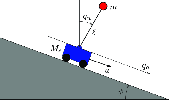
Figure 2: The cart-pendulum on an inclined plane.

The dynamics of the system has the form (1) with $n=2$, $q_{a}$ the position of the car, $q_{u}$ the angle of the pendulum with respect to the up-right vertical position and $u$ a force on the cart. The inertia matrix is

$$M(q_{u})=\left[\begin{array}[]{cc}m\ell^{2}&m\ell\cos(q_{u}-\psi)\\ m\ell\cos(q_{u}-\psi)&M_{c}+m\end{array}\right],$$

with $M_{c},m$ the masses of the cart and pendulum, respectively, $\ell$ the pendulum length and $\psi$ the angle of inclination of the plane. The potential energy function is

$$V(q)=mg\ell\cos(q_{u})-(M_{c}+m)g\sin(\psi)q_{a},$$

and the input matrix is $G=\mbox{col}(0,1)$. The desired equilibrium is $(0,q_{a}^{\star})$ with $q_{a}^{\star}\in\mathbb{R}$, which is the only constant assignable equilibrium point.

This system clearly satisfies Assumptions A1-A4 and A8 with $s_{a}=-(M_{c}+m)g\sin(\psi)$ and $c_{0}=0$. Applying Proposition 1 we identify the cyclo–passive outputs as

$$y_{a} =\dot{q}_{a}+\frac{m\ell}{M_{c}+m}\cos(q_{u}-\psi)\dot{q}_{u}$$

$$y_{u} =-\frac{m\ell}{M_{c}+m}\cos(q_{u}-\psi)\dot{q}_{u}.$$

The signal $y_{d}$ defined in (14) takes the form

$$y_{d}=k_{a}\dot{q}_{a}+(k_{a}-k_{u})\frac{m\ell}{M_{c}+m}\cos(q_{u}-\psi)\dot{q}_{u}.$$

Assumption A6 is also satisfied with

$$V_{N}(q_{u})=\frac{m\ell}{M_{c}+m}\sin(q_{u}-\psi).$$

Finally, from Proposition 2 the PID controller is given by (13) where the integral term (26) takes the form

$$z_{1}=k_{a}q_{a}+(k_{a}-k_{u})\frac{m\ell}{M_{c}+m}\sin(q_{u}-\psi)+\kappa,$$

and

$$S(q,\dot{q}) =-k_{u}K_{D}\Bigg{\{}-\frac{m\ell}{M_{c}+m}\sin(q_{u}-\psi)\dot{q}_{u}^{2}+\mathcal{N}(q_{u})\left[-m\ell\sin(q_{u}-\psi)\dot{q}_{u}^{2}-(M_{c}+m)g\sin(\psi)\right]$$

$$+ \frac{m^{2}\ell^{2}g}{M_{c}+m}(m_{uu}^{s})^{-1}\cos(q_{u}-\psi)\sin(q_{u})\Bigg{\}}+k_{a}K_{D}g\sin(\psi),$$

$$\mathcal{N}(q_{u}) =\frac{m\cos^{2}(q_{u}-\psi)}{(M_{c}+m)\left[M_{c}+m-m\cos^{2}(q_{u}-\psi)\right]},$$

$$K(q_{u}) =-\frac{k_{u}K_{D}m\left[\cos(q_{u}-\psi)\right]^{2}}{(M_{c}+m)\left(M_{c}+m\left[\sin(q_{u}-\psi)\right]^{2}\right)}+k_{e}+\frac{k_{a}K_{D}}{(M_{c}+m)},$$

$$\kappa =-k_{a}q_{a}^{\star}+(k_{a}-k_{u})\frac{m\ell\sin(\psi)}{M_{c}+m}.$$

The parameters and initial conditions used in the simulations have been chosen according to [4] and they are given as follows: $m=0.14$ $kg$, $M_{c}=0.44$ $kg$, $l=0.215$ $m$, $\psi=20$ degrees, $q(0)=(20$deg$,-0.6$m) and $\dot{q}(0)=0$. The desired equilibrium is set to $q_{a}^{\star}=0$ $m$ for $t\in(0,5)$ and to $q_{a}^{\star}=-0.3$ $m$ for $t\in(5,10)$, with $q_{u}^{\star}=0$ always.

The gains of the PID-PBC (13) are chosen as $K_{D}=0.1$, $K_{P}=1$ and $K_{I}=2$. Using these values we present three set of simulations where we change one-by-one the gains $k_{a}$, $k_{u}$ and $k_{e}$ while keeping the PID-PBC gains unaltered—always satisfying Assumptions A5 and A7. Variations of the PID-PBC gains were also considered but their effect was less informative than changing the gains $k_{a},k_{u}$ and $k_{e}$ In all cases we present the transient behavior of $q$, $\dot{q}$, $u$ and the factor $K(q_{u})$. Figs. 3-5 correspond to variations of $k_{a}$ with $k_{u}=-500$ and $k_{e}=5$. In Figs. 6-8 we change now $k_{u}$ with $k_{a}=50$ and $k_{e}=5$. Finally, Figs. 9-11 correspond to variations of $k_{e}$ with $k_{a}=50$ and $k_{u}=-500$. In all cases, the desired regulation objective is achieved very fast with a reasonable control effort.

These plots should be compared with Fig. 5 in [4] where the transient peaks are much larger and they take over $100$ $s$ to die out. Unfortunately, the plots of the control signal are not shown in [4], but given the magnitudes selected in the controller it is expected to be much larger than the ones resulting from the PID-PBC.

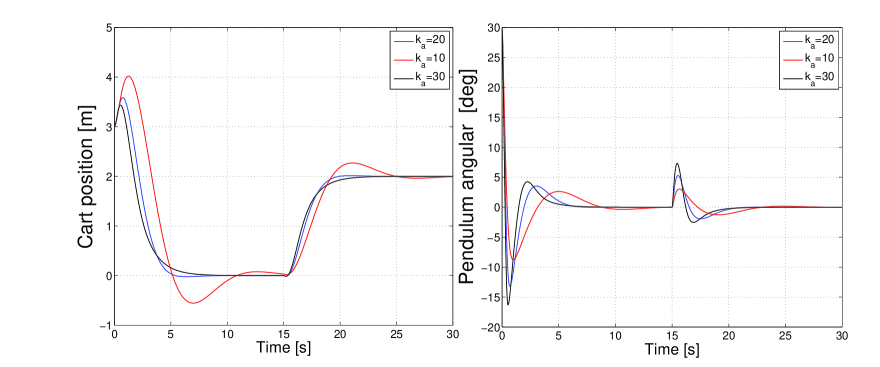
Figure 3: Time histories of the position of the cart $q_{a}(t)$ and angle of the pendulum $q_{u}(t)$.

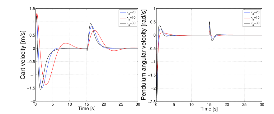
Figure 4: Time histories of the velocity of the cart $\dot{q}_{a}(t)$ and angular velocity of the pendulum $\dot{q}_{u}(t)$.

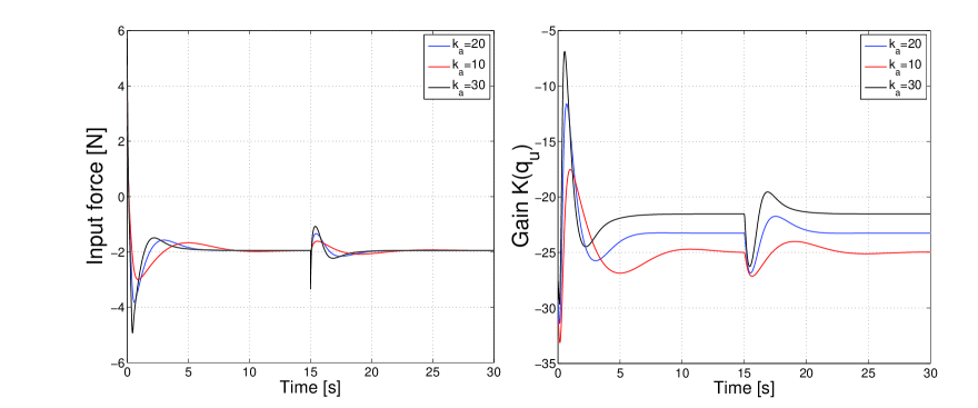
Figure 5: Time histories of the input force $u(t)$ and the nonlinear gain $K(q_{u})$.

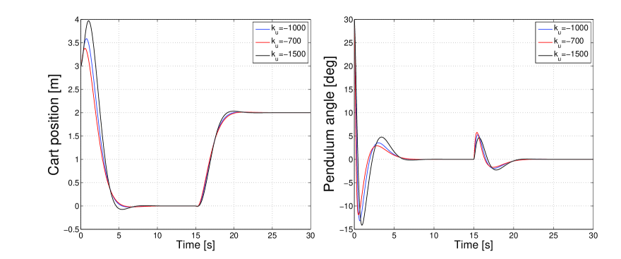
Figure 6: Time histories of the position of the cart $q_{a}(t)$ and angle of the pendulum $q_{u}(t)$.

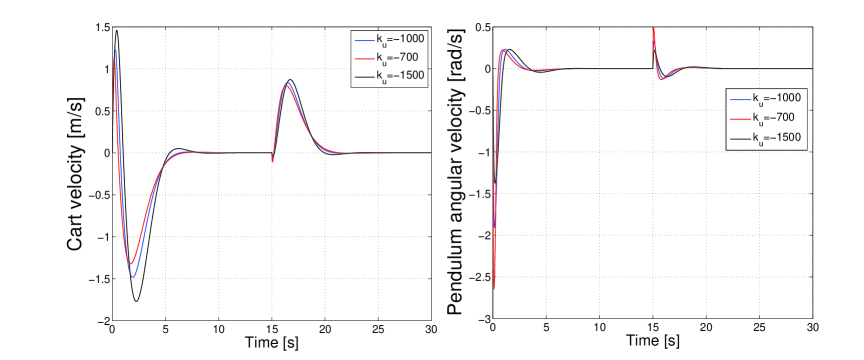
Figure 7: Time histories of the velocity of the cart $\dot{q}_{a}(t)$ and angular velocity of the pendulum $\dot{q}_{u}(t)$.

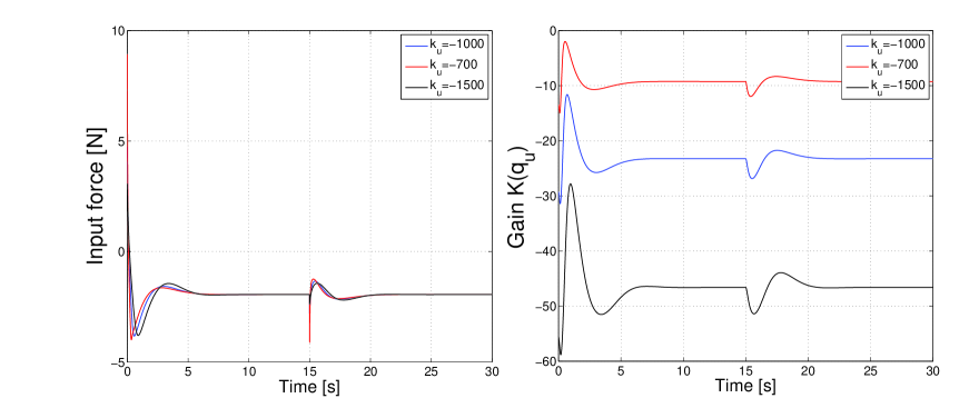
Figure 8: Time histories of the input force $u(t)$ and the nonlinear gain $K(q_{u})$.

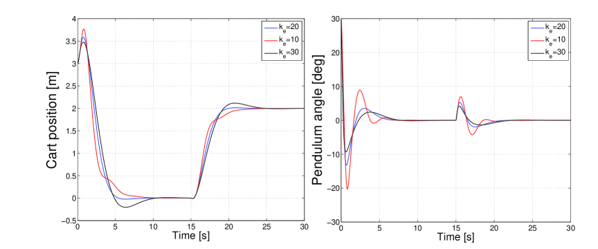
Figure 9: Time histories of the position of the cart $q_{a}(t)$ and angle of the pendulum $q_{u}(t)$.

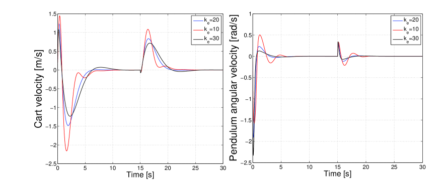
Figure 10: Time histories of the velocity of the cart $\dot{q}_{a}(t)$ and angular velocity of the pendulum $\dot{q}_{u}(t)$.

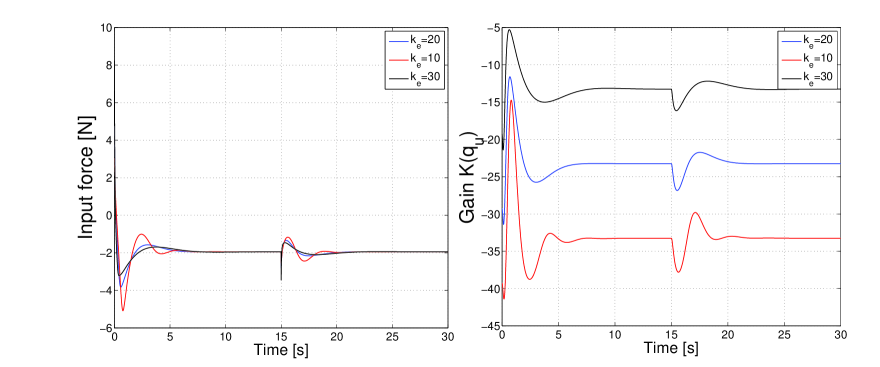
Figure 11: Time histories of the input force $u(t)$ and the nonlinear gain $K(q_{u})$.

Finally, we present in Fig. 12 a serie of captures of a video animation of the cart-pendulum with initial conditions $(q(0),\dot{q}(0))=(20$deg, -$0.6$m), $\dot{q}(0)=0$ and desired equilbirum at the origin. The controller gains were selected as follows: $k_{a}=50$, $k_{u}=-450$, $k_{e}=5$, $K_{D}=0.1$, $K_{P}=1$ and $K_{I}=2$. As it can be seen in the animation the PID-PBC ensures very good performance while satisfying Assumptions A5 and A7.

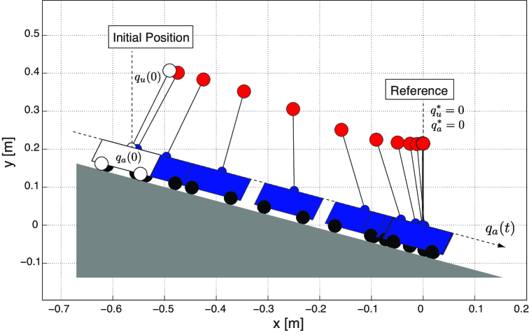
Figure 12: Captures of a video animation of the cart-pendulum on an inclined plane. The full-video animation can be watched in https://youtu.be/CGInoXkR0FA.

7 Conclusions and Future Research

We have identified in this paper a class of underactuated mechanical systems whose constant position can be stabilized with a linear PID controller. It should be underscored that in view of the freedom in the choice of the signs of the constants entering into the control design, i.e., $k_{e},k_{a}$ and $k_{u}$, the proposed PID is far from being standard. Given the popularity and simplicity of this controller, and the fact that the class contains some common benchmark examples, the result is of practical interest. Moreover, from the theoretical view point, the performance of the PID controllers sometimes parallels the one of total energy shaping controllers like IDA PBC. For instance, it has been proved that in some benchmark examples (like the cart-pendulum system and the inertia wheel), the desired equilibrium has the same estimated domain of attraction for both designs [7, 20]. See also the example of Subsection 6.2 where it is shown, via simulations, that the transient performance of the PID-PBC is far superior to the one of the total energy shaping controller reported in [4].

Besides the usual Lyapunov stability analysis, that imposes some constraints on the PID tuning gains to shape the energy function, a LaSalle-based study of attractivity has been carried out under strictly weaker conditions on these gains, but imposing the stronger Assumption A9 on the system. An additional contribution of the paper is the proof that it is possible to obviate the cancellation of the actuated part of the potential energy, provided this is described by an affine function—as indicated in Assumption A8.

Current research is under way along the following directions.

• To replace Assumption A8, which is rather restrictive, by some integrability-like condition that is verified in some practical examples.

• Investigate alternatives to the classical LaSalle analysis used in the proof of Proposition 5 to relax the restrictive assumption of injectivity of $\nabla V_{u}(q_{u})$, e.g., invoking the Matrosov-like theorems of [21]. Also, to identify classes of systems for which it is possible to prove boundedness of trajectories without Lyapunov stability.

• The theoretical analysis of the practical implementation of the PID using an approximate differentiator (19) seems feasible using singular perturbation arguments. However, as usual with this approach, the resulting results might be too conservative to be of practical interest.

• It is necessary to get a better understanding—hopefully in some geometric or coordinate-free terms—of the class of systems verifying the key Assumptions A1-A4.

• To further explore the relationship between total energy shaping PBC and the proposed PID the following two questions should be explored.

  • Compare their transient performances, for instance, investigating the flexibility to locate the eigenvalues of their tangent approximations—as done in [14] for IDA-PBC.

  • In [8] it has been shown that the PID controller of [7] can be recasted as a classical IDA-PBC with generalized dissipative forces. What can be said about the nature of these forces?

A. Proof of Proposition 1

The first step in the proof is to invoke Assumptions A1-A4 to rewrite the system (1) in a more suitable form. Towards this end, we recall the following well–known identity given in eq. 3.19, page 72 of [13]

$$C(q,\dot{q})\dot{q}=\left[\nabla_{q}(M(q)\dot{q})-\frac{1}{2}\nabla_{q}^{\top}(M(q)\dot{q})\right]\dot{q},$$ (42)

Now, under Assumptions A2 and A3, the second function within brackets of the left hand side of (42) takes the form

$$\nabla_{q}(M\dot{q})=\left[\begin{array}[]{cc}\nabla_{q_{u}}(m_{au}^{\top}\dot{q}_{a}+m_{uu}\dot{q}_{u})&0_{s\times m}\\ \nabla_{q_{u}}(m_{au}\dot{q}_{u})&0_{m\times m}\end{array}\right],$$

where here, and throughout the rest of the proof, to simplify the notation, the arguments of some mappings will be omitted. Hence, using (A. Proof of Proposition 1), the vector (42) can be rewritten as follows

$$C\dot{q} = \left[\begin{array}[]{cc}\nabla_{q_{u}}(m_{au}^{\top}\dot{q}_{a}+m_{uu}\dot{q}_{u})-\frac{1}{2}\nabla^{\top}_{q_{u}}(m_{au}^{\top}\dot{q}_{a}+m_{uu}\dot{q}_{u})&-\frac{1}{2}\nabla^{\top}_{q_{u}}(m_{au}\dot{q}_{u})\\ \nabla_{q_{u}}(m_{au}\dot{q}_{u})&0_{m\times s}\end{array}\right]\dot{q}$$

$$= \left[\begin{array}[]{c}\nabla_{q_{u}}(m_{uu}\dot{q}_{u})\dot{q}_{u}-\frac{1}{2}\nabla^{\top}_{q_{u}}(m_{uu}\dot{q}_{u})\dot{q}_{u}+\nabla_{q_{u}}(m_{au}^{\top}\dot{q}_{a})\dot{q}_{u}-\frac{1}{2}\nabla^{\top}_{q_{u}}(m_{au}^{\top}\dot{q}_{a})\dot{q}_{u}-\frac{1}{2}\nabla^{\top}_{q_{u}}(m_{au}\dot{q}_{u})\dot{q}_{a}\\ \nabla_{q_{u}}(m_{au}\dot{q}_{u})\dot{q}_{u}\end{array}\right]$$

$$= \left[\begin{array}[]{c}\nabla_{q_{u}}(m_{uu}\dot{q}_{u})\dot{q}_{u}-\frac{1}{2}\nabla^{\top}_{q_{u}}(m_{uu}\dot{q}_{u})\dot{q}_{u}+\nabla_{q_{u}}(m_{au}^{\top}\dot{q}_{a})\dot{q}_{u}-\nabla^{\top}_{q_{u}}(m_{au}\dot{q}_{u})\dot{q}_{a}\\ \nabla_{q_{u}}(m_{au}\dot{q}_{u})\dot{q}_{u}\end{array}\right]$$

$$= \left[\begin{array}[]{c}C_{mu}(q_{u},\dot{q}_{u})\dot{q}_{u}+D_{mu}(q_{u},\dot{q})\\ \nabla_{q_{u}}(m_{au}\dot{q}_{u})\dot{q}_{u}\end{array}\right],$$

with

$$C_{mu}(q_{u},\dot{q}_{u}) := \nabla_{q_{u}}(m_{uu}\dot{q}_{u})-\frac{1}{2}\nabla^{\top}_{q_{u}}(m_{uu}\dot{q}_{u})$$ (47)

$$D_{mu}(q_{u},\dot{q}) := \nabla_{q_{u}}(m_{au}^{\top}\dot{q}_{a})\dot{q}_{u}-\nabla^{\top}_{q_{u}}(m_{au}\dot{q}_{u})\dot{q}_{a},$$ (48)

where we have used the fact that

$$\nabla_{q_{u}}^{\top}(m_{au}^{\top}\dot{q}_{a})\dot{q}_{u}=\nabla_{q_{u}}^{\top}(m_{au}\dot{q}_{u})\dot{q}_{a}.$$ (49)

Consequenty, invoking Assumption A4, the system (1) with the inner–loop control (4) can be written as

$$m_{uu}\ddot{q}_{u} = -[m_{au}^{\top}\ddot{q}_{a}+C_{mu}\dot{q}_{u}+D_{mu}+\nabla V_{u}]$$ (50)

$$\ddot{q}_{a} = -m_{aa}^{-1}[m_{au}\ddot{q}_{u}+\nabla_{q_{u}}(m_{au}\dot{q}_{u})\dot{q}_{u}-u].$$ (51)

Moreover, replacing (51) in (50), we get

$$m_{uu}^{s}\ddot{q}_{u} = m_{au}^{\top}m_{aa}^{-1}[\nabla_{q_{u}}(m_{au}\dot{q}_{u})\dot{q}_{u}-u]-[C_{mu}\dot{q}_{u}+D_{mu}+\nabla V_{u}]$$ (52)

We proceed now to prove (11). The time derivative of the storage function (6) along the solution of (52) yields

$$\quad\dot{H}_{u} = \dot{q}_{u}^{\top}\Big{[}m_{au}^{\top}m_{aa}^{-1}\Big{(}\nabla_{q_{u}}(m_{au}\dot{q}_{u})\dot{q}_{u}-u\Big{)}-\Big{(}C_{mu}\dot{q}_{u}+D_{mu}\Big{)}\Big{]}+{1\over 2}\dot{q}_{u}^{\top}\dot{m}_{uu}^{s}\dot{q}_{u}$$

$$= u^{\top}y_{u}+L(q,\dot{q})$$

where we used (5) and defined the matrix

$$L(q,\dot{q}):={1\over 2}\dot{q}_{u}^{\top}\Big{[}\dot{m}^{s}_{uu}+2m_{au}^{\top}m_{aa}^{-1}\nabla_{q_{u}}(m_{au}\dot{q}_{u})-2C_{mu}\Big{]}\dot{q}_{u}-\dot{q}_{u}^{\top}D_{mu}.$$ (53)

To complete the proof we will show that $L(q,\dot{q})=0$. This is established using Assumption A3, (49), the definition of $m_{uu}^{s}$ given in (10) and the following identities

$$\dot{q}_{u}^{\top}D_{mu} = 0$$

$$\dot{q}_{u}^{\top}[\dot{m}_{uu}-2C_{mu}]\dot{q}_{u} = 0$$

$$\dot{q}_{u}^{\top}\left[\frac{d}{dt}(m_{au}^{\top}m_{aa}^{-1}m_{au})-2m_{au}^{\top}m_{aa}^{-1}\nabla_{q_{u}}(m_{au}\dot{q}_{u})\right]\dot{q}_{u} = 0.$$

To prove (12) we, first, notice that the storage function (7) can be rewritten as follows

$$H_{a} = {1\over 2}\dot{q}^{\top}M_{a}\dot{q}\pm H_{u}$$ (54)

$$= {1\over 2}\dot{q}^{\top}M\dot{q}-H_{u}+V_{u}(q_{u}).$$

Hence, taking the time derivative of (54) along the solutions of (1) with the inner–loop control (4) yields

$$\dot{\bar{H}}_{a} = {1\over 2}\dot{q}^{\top}\dot{M}\dot{q}+\dot{q}^{\top}\left(-C(q,\dot{q})\dot{q}-\left[\begin{array}[]{c}\nabla V_{u}\\ u\end{array}\right]\right)-\dot{H}_{u}+\nabla V_{u}^{\top}\;\dot{q}_{u}$$

$$= \dot{q}_{a}^{\top}u-\dot{H}_{u}$$

$$= \dot{q}_{a}^{\top}u-y_{u}^{\top}u$$

$$= u^{\top}y_{a}.$$

$\Box\Box\Box$

B. Proof of Proposition 4

The proof follows very closely the proof of Proposition 1 with the only difference of the inclusion of $V_{a}(q_{a})$ via Assumption A8. Taking the time derivatives of the storage functions (38) along the solutions of (52) yields

$$\quad\dot{\bar{H}}_{u} = \dot{q}_{u}^{\top}\Big{[}m_{au}^{\top}m_{aa}^{-1}[\nabla_{q_{u}}(m_{au}\dot{q}_{u})\dot{q}_{u}+\nabla V_{a}-\tau]-(C_{mu}\dot{q}_{u}+D_{mu}+\nabla V_{u})\Big{]}+{1\over 2}\dot{q}_{u}^{\top}\dot{m}_{uu}^{s}\dot{q}_{u}$$

$$+\nabla V_{u}^{\top}\dot{q}_{u}-\dot{V}_{0}$$

$$= \tau^{\top}y_{u}+L(q,\dot{q})-\dot{V}_{0}+\kappa^{\top}y_{u}$$

$$= \tau^{\top}y_{u}$$

where $L(q,\dot{q})$ is given by (53), the second identity is obtained recalling that $L(q,\dot{q})=0$ and invoking A8, and the last one follows from (40).

We now proceed to prove passivity of the operator $\tau\mapsto y_{a}$. Similarly to (54) the storage function (39) can be rewritten as

$$\bar{H}_{a} = {1\over 2}\dot{q}M_{a}\dot{q}+V_{a}(q_{a})+V_{0}(q_{u})\pm\bar{H}_{u}$$

$$= {1\over 2}\dot{q}M\dot{q}+V_{a}(q_{u})+V_{0}(q_{u})+\left({1\over 2}\dot{q}_{u}m_{uu}^{s}\dot{q}_{u}+V_{u}(q_{u})-V_{0}(q_{u})\right)-\bar{H}_{u}$$

$$= {1\over 2}\dot{q}M\dot{q}-\bar{H}_{u}+V_{a}(q_{a})+V_{u}(q_{u}),$$

and computing its time derivatives along the solutions of (1) we get

$$\dot{\bar{H}}_{a} = \dot{q}^{\top}\left(-C(q,\dot{q})\dot{q}-\left[\begin{array}[]{c}\nabla V_{u}\\ \nabla V_{a}\end{array}\right]+\left[\begin{array}[]{c}0\\ \tau\end{array}\right]\right)+{1\over 2}\dot{q}^{\top}\dot{M}\dot{q}-\dot{\bar{H}}_{u}+\nabla^{\top}V_{a}\;\dot{q}_{a}+\nabla V_{u}^{\top}\;\dot{q}_{u}$$

$$= \dot{q}_{a}^{\top}\tau-\dot{\bar{H}}_{u}-\dot{q}_{u}^{\top}\nabla V_{u}+\nabla^{\top}V_{u}\;\dot{q}_{u}-\dot{q}_{a}^{\top}\nabla V_{a}+\nabla^{\top}V_{a}\;\dot{q}_{a}$$

$$= \dot{q}_{a}^{\top}\tau+\dot{q}_{u}^{\top}m_{au}^{\top}m_{aa}^{-1}\tau$$

$$= \tau^{\top}y_{a}.$$

$\Box\Box\Box$

C. Proof of Proposition 5

It has been shown in Subsection 4.2 that, independently of Assumption A7, the function $H_{d}(q,\dot{q})$ given in (35) verifies

$$\dot{H}_{d}=-\|y_{d}\|^{2}_{K_{P}},$$

where $y_{d}$ is defined in (15). Invoking La Salle’s invariance principle [11], we can conclude that all bounded trajectories converge to the maximum invariant set contained in

$$\mathcal{X}:=\{(q,\dot{q})\in\mathbb{R}^{n}\times\mathbb{R}^{n}\;|\;k_{a}\dot{q}_{a}+(k_{a}-k_{u})m_{aa}^{-1}m_{au}(q_{u})\dot{q}_{u}\equiv 0\}.$$

Now, from the PID controller (13) it is clear that $y_{d}\equiv 0$ implies $z_{1}=c_{0}$ and, consequently, $u=c_{0}$ where here, and throughout the rest of the proof, $c_{0}$ denotes a (generic) constant vector (of suitable dimensions).

We now compute the time derivative of $y_{d}$, which results as follows

$$\dot{y}_{d} = (k_{a}-k_{u})m_{aa}^{-1}\nabla_{q_{u}}(m_{au}\dot{q}_{u})\dot{q}_{u}+(k_{a}-k_{u})m_{aa}^{-1}m_{au}\ddot{q}_{u}+k_{a}\ddot{q}_{a}$$

$$= (k_{a}-k_{u})m_{aa}^{-1}u+k_{u}\ddot{q}_{a},$$

where we have used (51) to get the second identity. From the equation above $\dot{y}_{d}=0$ and $u=c_{0}$ we conclude that, in $\mathcal{X}$, $\ddot{q}_{a}=c_{0}$ also. Since we are looking only at bounded trajectories this implies that $\ddot{q}_{a}=\dot{q}_{a}=0$ and $q_{a}=c_{0}$. Setting $\dot{q}_{a}=0$ and $y_{d}=0$ in (25) yields $\dot{V}_{N}(q_{u})=0$ that, replaced in (24) and invoking the full rank Assumption A9, allows us to conclude that $\dot{q}_{u}=0$, which implies that $q_{u}=c_{0}$. This proves that the only bounded trajectories living in the residual set $\mathcal{X}$ are of the form $(q(t),\dot{q}(t))=(\bar{q},0)$, with $\bar{q}$ a constant vector.

It only remains to prove that the only point $(\bar{q},0)$, which is invariant to the dynamics, is with $\bar{q}=q^{\star}$. This follows from injectivity of $\nabla V_{u}(q_{u})$ that, setting it equal to zero, ensures $\bar{q}_{u}=q_{u}^{\star}$ and the following chain of implications

$$(q(t),\dot{q}(t))=(\bar{q},0) \Rightarrow u=0$$

$$\Rightarrow \bar{q}_{a}=q_{a}^{\star}$$

$$\Rightarrow \bar{q}=q^{\star},$$

where we have used (51) in the first implication and (29) together with $\bar{q}_{u}=q_{u}^{\star}$ in the second one.

$\Box\Box\Box$

References

- [1] J. Acosta, R. Ortega, A. Astolfi and I. Sarras, A Constructive Solution for Stabilization via Immersion and Invariance: The Cart and Pendulum System, Automatica, Vol. 44, No.9, pp. 2352-2357, 2008.
- [2] A. Astolfi, D. Karagiannis and R. Ortega, Nonlinear and Adaptive Control Design with Applications, Springer-Verlag, London, 2007.
- [3] K. J. Astrom and T. Hagglund, The Future of PID Control, Control Engineering Practice, Vol. 9, No. 11, pp. 1163-1175, 2001.
- [4] A. M. Bloch, D.E. Chang, N. E. Leonard and J.E. Marsden, Controlled Lagrangians and the Stabilization of Mechanical Systems II: Potential Shaping, IEEE Transactions on Automatic Control, Vol. 46, No. 10, pp. 1556-1571, 2001.
- [5] F. Bullo and A. D. Lewis, Geometric Control of Mechanical Systems, Springer-Verlag, New York-Heidelberg-Berlin, 2004.
- [6] C. A. Desoer and M. Vidyasagar, Feedback Systems: Input–Output Properties, Academic Press, New York, 1975.
- [7] A. Donaire, R. Mehra, R. Ortega, S. Satpute, J. G. Romero, F. Kazi and N. M. Singh, Shaping the Energy of Mechanical Systems Without Solving Partial Differential Equations, IEEE Transactions on Automatic Control, Vol. 61, No. 4, pp. 1051-1056, 2016.
- [8] A. Donaire, R. Ortega and J. G. Romero, Simultaneous Interconnection and Damping Assignment Passivity–Based Control of Mechanical Systems Using Dissipative Forces, Systems and Control Letters, Vol. 94, pp. 118-126, 2016.
- [9] K. Fujimoto and T. Sugie, Canonical Transformations and Stabilization of Generalized Hamiltonian Systems, Systems and Control Letters, Vol. 42, No. 3, pp. 217–227, 2001.
- [10] T. Hatanaka, N. Chopra, M. Fujita, and M. W. Spong, Passivity–Based Control and Estimation in Networked Robotics, Springer International, Cham, Switzerland, 2015.
- [11] H. K. Khalil, Nonlinear Systems, Third Edition, Prentice Hall, 2002.
- [12] R. Kelly and R. Ortega, Adaptive Control of Robot Manipulators: An Input-Output Approach, IEEE International Conference on Robotics and Automation, Philadelphia, PA, USA, 1988.
- [13] R. Kelly, V. Santibáñez and A. Loria, Control of Robot Manipulators in Joint Space, Springer, London, 2005.
- [14] P. Kotyczka, Local Linear Dynamics Assignment in IDA-PBC, Automatica, Vol. 49, No. 4, pp. 1037-1044, 2013.
- [15] R. Olfati-Saber, Nonlinear Control of Underactuated Mechanical Systems with Application to Robotics and Aerospace Vehicles, Phd Thesis, Department of Electrical Engineering and Computer Science, MIT, 2001.
- [16] R. Olfati-Saber, Normal Forms for Underactuated Mechanical Systems with Symmetry, IEEE Transactions on Automatic Control, Vol. 47, No. 2, pp. 305-308, 2002.
- [17] R. Ortega and E. Panteley, Adaptation is Unnecessary in Adaptive Control, IEEE Control Systems Magazine, Vol. 36, No. 1, pp. 47-52, 2016.
- [18] R. Ortega and M. W. Spong, Adaptive Motion Control of Rigid Robots: A tutorial, Automatica, Vol. 25, No.6, pp. 877-888, 1989.
- [19] R. Ortega, A. Donaire and J. G. Romero, Passivity–Based Control of Mechanical Systems, in Feedback Stabilization of Controlled Dynamical Systems–In Honor of Laurent Praly, ed. N. Petit, Springer, 2016.
- [20] J. G. Romero, R. Ortega A. Donaire. Energy Shaping of Mechanical Systems via PID Control and Extension to Constant Speed Tracking, IEEE Transactions on Automatic Control (To appear).
- [21] G. Scarciotti, L. Praly and A. Astolfi, Invariance-Like Theorems and “lim inf" Convergence Properties, IEEE Transactions on Automatic Control, Vol. 61, No. 3, pp. 648-661, 2016.
- [22] M. Spong, Partial Feedback Linearization of Underactuated Mechanical Systems, IEEE International Conference Intelligent Robots and Systems, Munich, Germany, pp. 314-321, 1994.
- [23] M. Takegaki, and S. Arimoto, A New Feedback Method for Dynamic Control of Manipulators, Transactions of the ASME: Journal of Dynamic Systems, Measurement and Control, Vol. 103, No. 2, pp.119-125, 1981.
- [24] A. Venkatraman, R. Ortega, I. Sarras and A. van der Schaft, Speed Observation and Position Feedback Stabilization of Partially Linearizable Mechanical Systems, IEEE Transactions on Automatic Control, Vol. 55, No.5, pp. 1059–1074, 2010.