KGEval: Estimating Accuracy of Automatically Constructed Knowledge Graphs

Abstract

Automatic construction of large knowledge graphs (KG) by mining web-scale text datasets has received considerable attention recently. Estimating accuracy of such automatically constructed KGs is a challenging problem due to their size and diversity. This important problem has largely been ignored in prior research – we fill this gap and propose KGEval. KGEval binds facts of a KG using coupling constraints and crowdsources the facts that infer correctness of large parts of the KG. We demonstrate that the objective optimized by KGEval is submodular and NP-hard, allowing guarantees for our approximation algorithm. Through extensive experiments on real-world datasets, we demonstrate that KGEval is able to estimate KG accuracy more accurately compared to other competitive baselines, while requiring significantly lesser number of human evaluations.

1 Introduction

Automatic construction of Knowledge Graphs (KGs) from Web documents has received significant interest over the last few years, resulting in the development of several large KGs consisting of hundreds of predicates (e.g., isCity, stadiumLocatedInCity(Stadium, City)) and millions of instances of such predicates called beliefs (e.g., (Joe Luis Arena, stadiumLocatedInCity, Detroit)). Examples of such KGs include NELL [24], Knowledge-Vault [8] etc.

Due to imperfections in the automatic KG construction process, many incorrect beliefs are also found in these KGs. Overall accuracy of a KG can quantify the effectiveness of its construction-process. Having knowledge of accuracy for each predicate in the KG can highlight its strengths and weaknesses and provide targeted feedback for improvement. Knowing accuracy at such predicate-level granularity is immensely helpful for Question-Answering (QA) systems that integrate opinions from multiple KGs [30]. For real-time QA-systems, being aware that a particular KG is more accurate than others in a certain domain, say sports, helps in restricting the search over relevant and accurate subsets of KGs, thereby improving QA-precision and response time. In comparison to the large body of recent work focused on construction of KGs, the important problem of accuracy estimation of such large KGs is unexplored – we address this gap in this paper.

True accuracy of a KG (or a predicate in the KG) may be estimated by aggregating human judgments on correctness of each and every belief in the KG (or predicate). Even though crowdsourcing marketplaces such as Amazon Mechanical Turk (AMT) provide a convenient way to collect human judgments, accumulating such judgments at the scale of larges KGs is prohibitively expensive. We shall refer to the task of manually classifying a single belief as true or false as a Belief Evaluation Task (BET). Thus, the crucial problem is: How can we select a subset of beliefs to evaluate which will give the best estimate of true (but unknown) accuracy of the overall KG and various predicates in it?

A naive and popular approach is to evaluate randomly sampled subset of beliefs from the KG. Since random sampling ignores relational-couplings present among the beliefs, it usually results in oversampling and poor accuracy estimates. Let us motivate this through an example.

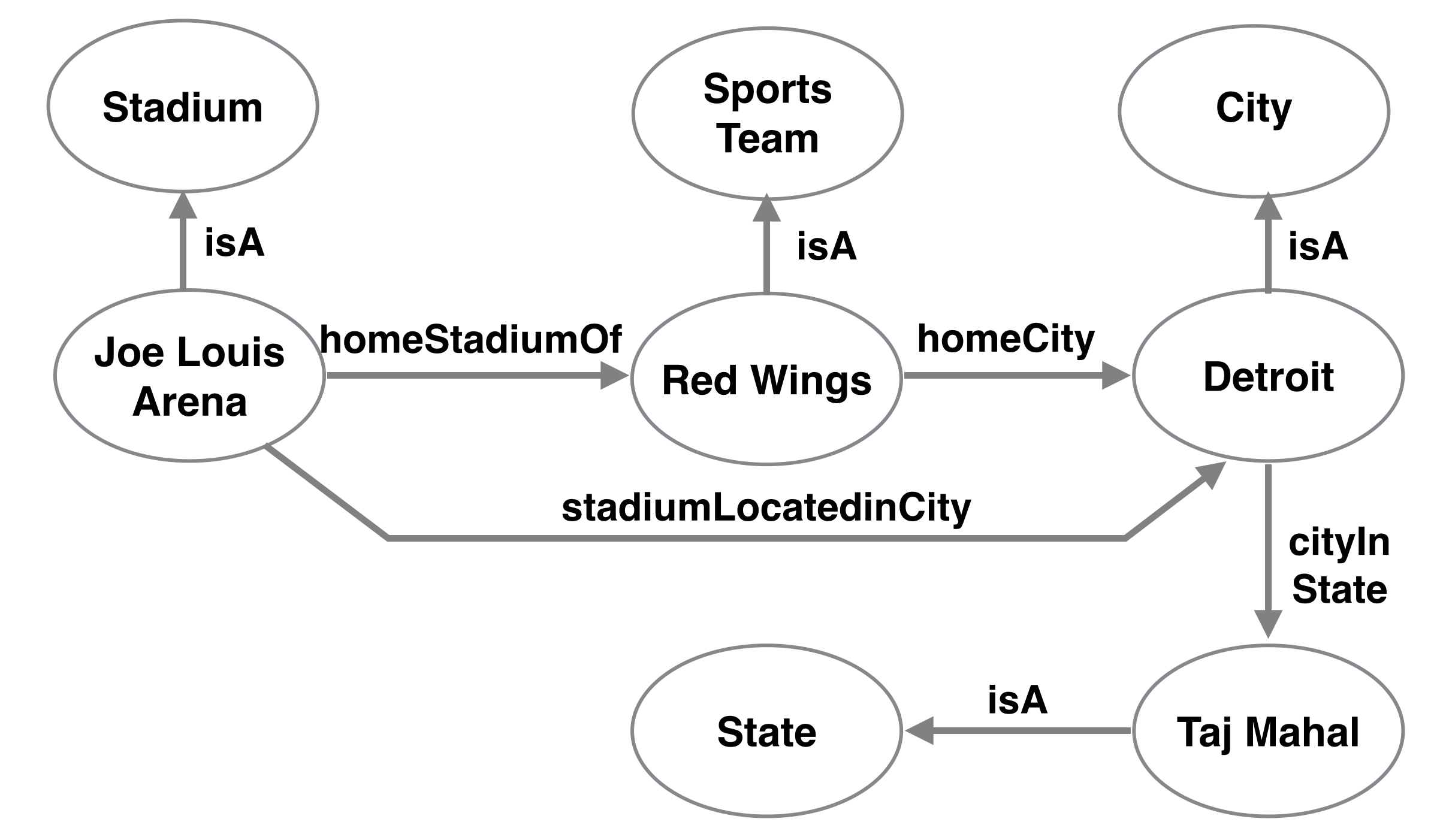
Figure 1: Knowledge Graph (KG) fragment used as motivating example in the paper. KGEval, the method proposed in this paper, is able to estimate the true accuracy 75% of this KG by evaluating only three beliefs (out of 8). In contrast, random evaluation, a popular alternative, gives an estimate of 66.7% after evaluating same number of beliefs. Please see Section 1 for details.

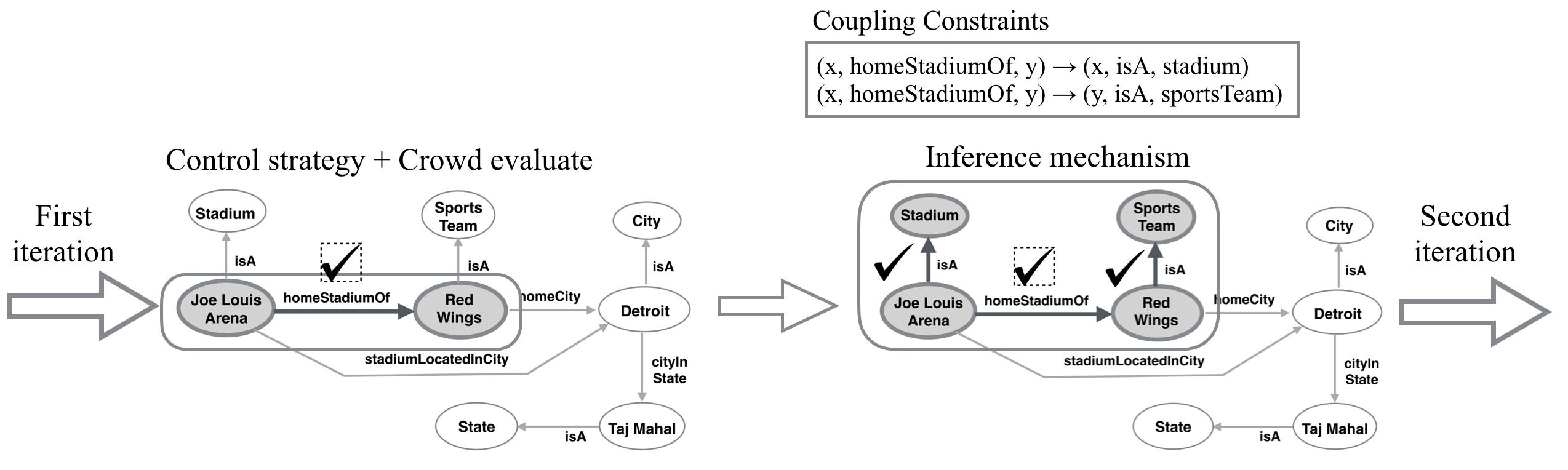
Figure 2: Demonstration of one iteration of KGEval. Control mechanism selects a belief whose correctness is evaluated from crowd. In the above example, (J.L. Arena, homeStadiumOf, Red Wings) is crowd-evaluated to be true (indicated by tick with dotted square). The inference mechanism take this evaluation along with coupling constraints among beliefs (Section 3.1) to infer correctness of other beliefs (shown by tick without square). All such crowdsourced and inferred evaluations are aggregated to get accuracy estimate. This iterative process continues until convergence. (Section 2.1 and Section 3).

Motivating example:

We motivate efficient accuracy estimation through the KG fragment shown in Figure 1. Here, each belief of the form (RedWings, isA, SportsTeam) is an edge in the graph. There are six correct and two incorrect beliefs (the two incident on Taj Mahal), resulting in an overall accuracy of $75\%(=6/8)$ which we would like to estimate. Additionally, we would also like to estimate accuracies of the predicates: homeStadiumOf, homeCity, stadiumLocatedInCity, cityInState and isA.

We now demonstrate how coupling constraints among beliefs may be exploited for faster and more accurate accuracy estimation. Type consistency is one such coupling constraint. For instance, we may know from KG ontology that the homeStadiumOf predicate connects an entity from the Stadium category to another entity in the Sports Team category. Now, if (Joe Louis Arena, homeStadiumOf, Red Wings) is sampled and is evaluated to be correct, then from these type constraints we can infer that (Joe Louis Arena, isA, Stadium) and (Red Wings, isA, Sports Team) are also correct. Similarly, by evaluating (Taj Mahal, isA, State) as false, we can infer that (Detroit, cityInState, TajMahal) is incorrect. Please note that even though type information may have been used during KG construction and thereby the KG itself is type-consistent, it may still contain incorrect type-related beliefs. An example is the (Taj Mahal, isA, State) belief in the type-consistent KG in Figure 1. Additionally, we have Horn-clause coupling constraints [24, 20], such as homeStadiumOf(x, y) $\land$ homeCity(y, z) $\rightarrow$ stadiumLocatedInCity(x, z). By evaluating (Red Wings, homeCity, Detroit) and applying this horn-clause to the already evaluated facts mentioned above, we infer that (Joe Louis Arena, stadiumLocatedInCity, Detroit) is also correct. We explore generalized forms of these constraints in Section 3.1.

Thus, evaluating only three beliefs, and exploiting constraints among them, we exactly estimate the overall true accuracy as $75\%$ and also cover all predicates. In contrast, the empirical accuracy by randomly evaluating three beliefs, averaged over 5 trials, is $66.7\%$.

Our contributions

We make the following contributions in this paper:

• Initiate a systematic study into the unexplored yet important problem of evaluation of automatically constructed Knowledge Graphs.

• We present KGEval, a novel crowdsourcing-based system for estimating accuracy of large knowledge graphs (KGs). KGEval exploits dependencies among beliefs for more accurate and faster KG accuracy estimation.

• Demonstrate KGEval’s effectiveness through extensive experiments on real-world KGs, viz., NELL [24] and Yago [32]. We also evaluate KGEval’s robustness and scalability.

All the data and code used in the paper will be made publicly available upon publication.

2 Overview and Problem Statement

2.1 KGEval: Overview

The core idea behind KGEval is to estimate correctness of as many beliefs as possible while evaluating only a subset of them using humans through crowdsourcing. KGEval achieves this using an iterative algorithm which alternates between the following two stages:

• Control Mechanism (Section 3.4): In this step, KGEval selects the belief which is to be evaluated next using crowdsourcing.

• Inference Mechanism (Section 3.3): Here KGEval uses coupling constraints and beliefs evaluated so far to automatically estimate correctness of additional beliefs.

This iterative process is repeated until there are no more beliefs to be evaluated, or until a pre-determined number of iterations are processed. One iteration of KGEval over the KG fragment from Figure 1 is shown in Figure 2. Firstly, KGEval’s control mechanism selects the belief (John Louis Arena, homeStadiumOf, Red Wings), whose evaluation is subsequently crowdsourced. Next, the inference mechanism uses the so evaluated belief and type coupling constraints (not shown in figure) to infer that (John Louis Arena, isA, Stadium) and (Red Wings, isA, Sports Team) are also true. In the next iteration, the control mechanism selects another belief for evaluation, and the process continues.

Symbol	Description
$\mathcal{H}{}=\{h_{1},\ldots,h_{n}\}$	Set of all $n$ Belief Evaluation Tasks (BETs)
$c(h)\in\mathbb{R}_{+}$	Cost of labeling $h$ from crowd
$\mathcal{C}{}=\{(\mathcal{C}{}_{i},\theta_{i})\}$	Set of coupling constraints $\mathcal{C}{}_{i}$ with weights $\theta_{i}\in\mathbb{R}_{+}$
$t(h)\in\{0,1\}$	True label of $h$
$l(h)\in\{0,1\}$	Estimated evaluation label of $h$
$\mathcal{H}{}_{i}=\mathrm{Dom}(\mathcal{C}_{i}{})$	$\mathcal{H}{}_{i}\subseteq\mathcal{H}{}$ which participate in $\mathcal{C}{}_{i}$
$G=(\mathcal{H}{}\cup\mathcal{C}{},\mathcal{E})$	Bipartite Evaluation Coupling Graph. $e\in\mathcal{E}$ between $\mathcal{H}{}_{j}$ and $\mathcal{C}{}_{j}$ denotes $\mathcal{H}{}_{j}\in\mathrm{Dom}(\mathcal{C}_{j}{})$ .
$\mathcal{Q}\subseteq\mathcal{H}{}$	BETs evaluated using crowd
$\mathcal{I}\big{(}G,\mathcal{Q}\big{)}\subseteq\mathcal{H}{}$	Inferable Set for evidence $\mathcal{Q}$: BETs for which labels can be inferred by inference algorithm
$\Phi(\mathcal{Q})=$ $~{}~{}~{}~{}~{}~{}~{}~{}\frac{1}{|\mathcal{Q}|}\sum_{h\in\mathcal{Q}}t(h)$	True accuracy of evaluated BETs $\mathcal{Q}$

Table 1: Summary of notations used (Section 2.2).

2.2 Notations and Problem Statement

We are given a KG with $n$ beliefs. Evaluating a single belief as true or false forms a Belief Evaluation Task (BET). Coupling constraints are derived by determining relationships among BETs, which we further discuss in Section 3.1. Notations used in the rest of the paper are summarized in Table 1.

Inference algorithm helps us work out evaluation labels of other BETs using constraints $\mathcal{C}{}$. For a set of already evaluated BETs $\mathcal{Q}\subseteq\mathcal{H}{}$, we define inferable set $\mathcal{I}\big{(}G,\mathcal{Q}\big{)}\subseteq\mathcal{H}{}$ as BETs whose evaluation labels can be deduced by the inference algorithm. We calculate the average true accuracy of a given set of evaluated BETs $\mathcal{Q}\subseteq\mathcal{I}\big{(}G,\mathcal{Q}\big{)}\subseteq\mathcal{H}$ by $\Phi(\mathcal{Q})=\frac{1}{|\mathcal{Q}|}\sum_{h\in\mathcal{Q}}t(h)$.

KGEval aims to sample and crowdsource a BET set $\mathcal{Q}$ with the largest inferable set, and solves the optimization problem:

$$\arg\max_{\mathcal{Q}\subseteq\mathcal{H}}~{}\left|\mathcal{I}\big{(}G,\mathcal{Q}\big{)}\right|$$ (1)

3 KGEval: Method Details

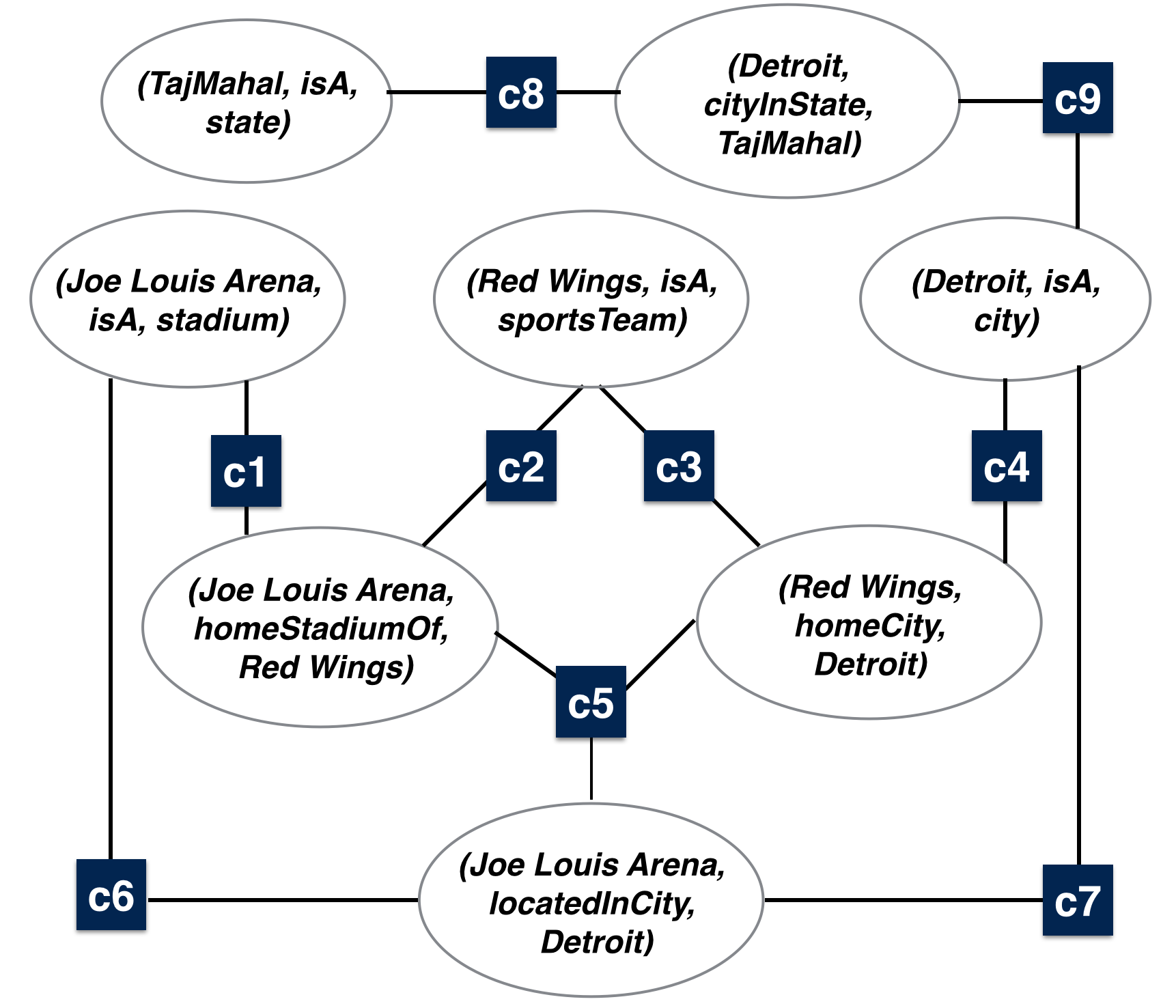
Figure 3: Evaluation Coupling Graph (ECG) constructed for example in Figure 1. Each edge (BET) in Figure 1 is represented as a node here. (Section 3.2)

In this section, we describe various components of KGEval. First, we present coupling constraint details in Section 3.1. Instead of working directly over the KG, KGEval combines all KG beliefs and constraints into an Evaluation Coupling Graph (ECG), and works directly with it. Construction of ECG is described in Section 3.2. Inference and Control mechanisms are then described in Section 3.3 and Section 3.4, respectively. The overall algorithm is presented in Algorithm 1.

3.1 Coupling Constraints

Beliefs are coupled in the sense that their truth labels are dependent on each other. We use any additional coupling information like metadata, KG-ontology etc., to derive coupling constraints that can help infer evaluation label of a BET based on labels of other BET(s). In this work, we derive constraints $\mathcal{C}{}$ from the KG ontology and link-prediction algorithms, such as PRA [20] over NELL and AMIE [10] over Yago. These rules are jointly learned over entire KG with millions of facts and we assume them to be true. The alternative of manually identifying such complex rules would be very expensive and unfeasible.

We use conjunction-form first-order-logic rules and refer to them as Horn clauses. Examples of a few such coupling constraints are shown below.

$\mathcal{C}_{2}$: (x, homeStadiumOf, y) $\rightarrow$ (y, isA, sportsTeam)

$\mathcal{C}_{5}$: (x, homeStadiumOf, y) $\land$ (y, homeCity, z) $\to$ (x, stadiumLocatedInCity, z)

Each coupling constraint $\mathcal{C}{}_{i}$ operates over $\mathcal{H}{}_{i}\subseteq\mathcal{H}{}$ to the left of its arrow and infers label of the BET on the right of its arrow. BETs participating in $\mathcal{C}{}_{i}$ are referred to as its domain $\mathrm{Dom}(\mathcal{C}_{i}{})$. $\mathcal{C}_{2}$ enforces type consistency and $\mathcal{C}_{5}$ is an instance of PRA path that conveys if a stadium $S$ is home to a certain team $T$ based in city $C$, is itself located in city $C$. These constraints have also been successfully employed earlier during knowledge extraction [24] and integration [28].

Note that these constraints are directional and inference propagates in forward direction. For example, inverse of $\mathcal{C}_{2}$, i.e., correctness of (RedWings, isA, sportsTeam) does not give any information about the correctness of (JoeLouisArena, homeStadiumOf, RedWings).

3.2 Evaluation Coupling Graph (ECG)

Given $\mathcal{H}{}$ and $\mathcal{C}{}$, we construct a graph with two types of nodes: (1) a node for each BET $h\in\mathcal{H}{}$, and (2) a node for each constraint $\mathcal{C}{}_{i}\in\mathcal{C}{}$. Each $\mathcal{C}{}_{i}$ node is connected to all $h$ nodes that participate in it. We call this graph the Evaluation Coupling Graph (ECG), represented as $G=(\mathcal{H}{}\cup\mathcal{C}{},\mathcal{E})$ with set of edges $\mathcal{E}=\{(\mathcal{C}{}_{i},h)~{}|~{}h\in\mathrm{Dom}(\mathcal{C}{}_{i})~{}\forall\mathcal{C}{}_{i}\in\mathcal{C}\}$. Note that ECG is a bipartite factor graph [19] with $h$ corresponding to variable-nodes and $\mathcal{C}_{i}{}$ corresponding to factor-nodes.

Figure 3 shows ECG constructed out of the motivating example in Figure 1 with $|\mathcal{C}{}|=8$ and separate nodes for each of the edges (beliefs or BETs) in KG. We pose the KG evaluation problem as classification of BET nodes in the ECG by allotting them a label of $1$ or $0$ to represent true or false respectively.

3.3 Inference Mechanism

Inference mechanism helps propagate true/false labels of evaluated beliefs to other non-evaluated beliefs using available coupling constraints [5]. We use Probabilistic Soft Logic (PSL) [6] as our inference engine to implement propagation of evaluation labels. PSL is a declarative language to reason uncertainty in relational domains via first order logic statements. Below we briefly describe the internal workings of PSL with respect to the accuracy estimation problem.

PSL Background

PSL relaxes each conjunction rule $\mathcal{C}_{j}{}$ to $\mathbb{R}{}$ using Lukaseiwicz t-norms: $a\land b\to max\{0,a+b-1\}$. Potential function $\psi_{j}$ is defined for each $\mathcal{C}_{j}{}$ using this norm and it depicts how satisfactorily constraint $\mathcal{C}_{j}{}$ is satisfied. For example, $\mathcal{C}_{5}$ mentioned earlier is transformed from first-order logical form to a real valued number by

$$\psi_{j}(\mathcal{C}_{5}{})=\big{(}\max\{0,h_{x}+h_{y}-1-h_{w}\}\big{)}^{2}$$ (2)

where $\mathcal{C}_{5}{}=h_{x}\land h_{y}\to h_{w}$, where $h_{x}$ denotes the evaluation score $\in[0,1]$ associated with the BET (Joe Louis Arena, homeStadiumOf, Red Wings), $h_{y}$ corresponds to (Red Wings, homeCity, Detroit) and $h_{w}$ to (Joe Louis Arena, locatedInCity, Detroit). Higher value of potential function $\psi_{j}$ represents lower fit for constraint $\mathcal{C}_{j}{}$.

The probability distribution over label assignment is so structured such that labels which satisfy more coupling constraints are more probable. Probability of any label assignment $\Omega\big{(}\mathcal{H}{}\big{)}\in\{0,1\}^{|\mathcal{H}{}|}$ over BETs in $G$ is given by

$$\mathbb{P}\big{(}\Omega\big{(}\mathcal{H}{}\big{)}\big{)}=\frac{1}{Z}\exp\Big{[}-\sum\limits_{j=1}^{|\mathcal{C}{}|}\theta_{j}\psi_{j}\big{(}\mathcal{C}_{j}{}\big{)}\Big{]}$$ (3)

where $Z$ is the normalizing constant and $\psi_{j}$ corresponds to potential function acting over BETs $h\in\mathrm{Dom}(\mathcal{C}_{j}{})$. Final assignment of $\Omega(\mathcal{H}{})_{PSL}\in\{1,0\}^{|\mathcal{H}{}|}$ labels is obtained by solving the maximum a-posteriori (MAP) optimization problem

$\Omega\big{(}\mathcal{H}{}\big{)}_{PSL}=\operatorname*{arg\,max}\limits_{\Omega(\mathcal{H}{})}~{}\mathbb{P}\bigg{(}\Omega\big{(}\mathcal{H}{}\big{)}\bigg{)}$

We denote by $M_{PSL}(h,\gamma)\in[0,1]$ the PSL-estimated score for label $\gamma\in\{1,0\}$ on BET $h$ in the optimization above.

Inferable Set using PSL: We define estimated label for each BET $h$ as shown below.

$$l(h)=\begin{cases}1~{}~{}\mathrm{if}~{}~{}M_{PSL}(h,1)\geq\tau\\ 0~{}~{}\mathrm{if}~{}~{}M_{PSL}(h,0)\geq\tau\\ \varnothing~{}~{}\mathrm{otherwise}\end{cases}$$

where threshold $\tau$ is system hyper-parameter. Inferable set is composed of BETs for which inference algorithm (PSL) confidently propagates labels.

$\mathcal{I}(G,\mathcal{Q})=\{h\in\mathcal{H}{}~{}|~{}l(h)\neq\varnothing\}$

Note that two BET nodes from ECG can interact with varying strengths through different constraint nodes; this multi-relational structure requires soft probabilistic propagation.

3.4 Control Mechanism

Control mechanism selects the BET to be crowd-evaluated at every iteration. We first present the following two theorems involving KGEval’s optimization in Equation (1). Please refer to the Appendix for proofs of both theorems.

Submodularity

Theorem 1.

The function optimized by KGEval (Equation (1)) using the PSL-based inference mechanism is submodular [23].

Intuitively, the amount of additional utility, in terms of label inference, obtained by adding a BET to larger set is lesser than adding it to any smaller subset. The proof follows from the fact that all pairs of BETs satisfy the regularity condition [12, 17], further used by a proven conjecture [16, 25]. Refer Appendix Section A for detailed proof.

NP-Hardness

Theorem 2.

The problem of selecting optimal solution in KGEval’s optimization (Equation (1)) is NP-Hard.

Proof follows by reducing NP-complete Set-cover Problem (SCP) to selecting $\mathcal{Q}$ which covers ${\mathcal{I}}(G,\mathcal{Q})$.

Given a partially evaluated ECG, the control mechanism aims to select the next set of BETs which should be evaluated by the crowd. However, before going into the details of the control mechanism, we state a few properties involving KGEval’s optimization in Equation (1).

Justification for Greedy Strategy

From Theorem 1 and 2, we observe that the function optimized by KGEval is NP-hard and submodular. Results from [27] prove that greedy hill-climbing algorithms solve such maximization problem within an approximation factor of $(1-1/e)\approx$ 63% of the optimal solution. Hence, we adopt a greedy strategy as our control mechanism. We iteratively select the next BET which gives the greatest increase in size of inferable set.

In this work, we do not integrate all aspects crowdsourcing techniques like aggregating labels, worker’s quality estimation etc. However, we acknowledge their importance and hope to pursue them in our future works. In Appendix A.1, we present a majority-voting based mechanism to handle noisy crowd workers under limited budget. We propose a strategy to redundantly post each BET to multiple workers and bound their estimation error.

Algorithm 1 KGEval: Accuracy Estimation of Knowledge Graphs

0:  $\mathcal{H}$: BETs, $\mathcal{C}$: coupling constraints, $\mathbb{B}$: assigned budget, $\mathcal{S}$: seed set, $c(h)$: BET cost function, $\Phi$: BET categorization score aggregator

1:  $G=\mbox{{BuildECG}}(\mathcal{H}{},\mathcal{C}{})$

2:  $B_{r}=\mathbb{B}$

3:  $\mathcal{Q}_{0}=\mathcal{S}$, $t=1$

4:  repeat

5:     $h^{*}=\arg\max_{h\in\mathcal{H}-Q}\left|\mathcal{I}(G,\mathcal{Q}_{t-1}\cup\{h\})\right|$

6:     $\mbox{{CrowdEvaluate}}(h^{*})$

7:     $\mbox{{RunInference}}(\mathcal{Q}_{t-1}\cup h^{*})$

8:     $\mathcal{Q}_{t}=\mathcal{I}(G,\mathcal{Q}_{t-1}\cup\{h^{*}\})$

9:     $B_{r}=B_{r}-c(h^{*})$

10:     $\mathcal{Q}=\mathcal{Q}\cup\mathcal{Q}_{t}$

11:     if $\mathcal{Q}\equiv\mathcal{H}$ then

12:        Exit

13:     end if

14:     $\mathrm{Acc_{t}}=\frac{1}{|\mathcal{Q}|}\sum_{h\in\mathcal{Q}}l(h)$

15:     $t=t+1$

16:  until Convergence

17:  return  $\mathrm{Acc_{t}}$

3.5 Bringing it All Together

Algorithm 1 presents KGEval. In Lines 1-3, we build the Evaluation Coupling Graph $G=(\mathcal{H}{}\cup\mathcal{C}{},\mathcal{E})$ and use the labels of seed set $\mathcal{S}$ to initialize $G$. In lines 4-16, we repetitively run our inference mechanism, until either the accuracy estimates have converged, or all the BETs are covered.

Convergence

In this paper, we define convergence whenever the variance of sequence of accuracy estimates [ $\mathrm{Acc_{t-k}}$, $\ldots$, $\mathrm{Acc_{t-1}}$, $\mathrm{Acc_{t}}$] is less than $\alpha$. We set $k=9$ and $\alpha=0.002$ for our experiments.

In each iteration, the BET with the largest inferable set is identified and evaluated using crowdsourcing (Lines 5-6). The new inferable set $\mathcal{Q}_{t}$ is estimated. These automatically annotated nodes are added to $\mathcal{Q}$ (Lines 7-10). Finally, average of all the evaluated BET scores is returned as the estimated accuracy.

4 Experiments

To assess the effectiveness of KGEval, we ask the following questions:

• How effective is KGEval in estimating KG accuracy, both at predicate-level and at overall KG-level? (Section 4.3).

• What is the effect of coupling constraints on its performance? (Section 4.4).

• And lastly, how robust is KGEval to estimating accuracy of KGs with varying quality? (Section 4.5).

4.1 Setup

Evaluation set	$\mathcal{H}{}_{N}$ (NELL)	$\mathcal{H}{}_{Y}$ (Yago2)
#BETs	$1860$	$1386$
#Constraints	$|\mathcal{C}_{N}|=130$	$|\mathcal{C}_{Y}|=28$
#Predicates	$18$	$16$
Gold Acc.	$91.34\%$	$99.20\%$

Table 2: Details of BET subsets used for accuracy evaluation. (Section 4.1).

4.1.1 Setup

Datasets

We consider two automatically constructed KGs, NELL and Yago2 for experiments. From NELL, we choose a sub-graph of sports related beliefs NELL-sports, mostly pertaining to athletes, coaches, teams, leagues, stadiums etc. We construct coupling constraints set $\mathbf{\mathcal{C}_{N}{}}$ using top-ranked PRA inference rules for available predicate-relations [20]. The confidence score returned by PRA are used as weights $\theta_{i}$. We use NELL-ontology’s predicate-signatures to get information for type constraints. We also select YAGO2-sample , which unlike NELL-sports, is not domain specific. We use AMIE horn clauses [10] to construct multi-relational coupling constraints $\mathbf{\mathcal{C}_{Y}{}}$. For each $\mathcal{C}_{i}{}$, the score returned by AMIE is used as rule weight $\theta_{i}$. Table 2 reports the statistics of datasets used, their true accuracy and number of coupling constraints.

Size of evaluation set

In order to calculate accuracy, we require gold evaluation of all beliefs in the evaluation set. Since obtaining gold evaluation of the entire (or large subsets of) NELL and Yago2 KGs will be prohibitively expensive, we sample a subset of these KGs for evaluation. Statistics of the evaluation datasets are shown in Table 2. We instantiated top ranked PRA and AMIE first-order-conjunctive rules over NELL-sports and Yago datasets respectively and their participating beliefs form $\mathcal{H}_{N}{}$ and $\mathcal{H}_{Y}{}$.

Initialization

Algorithm 1 requires initial seed set $\mathcal{S}$ which we generate by randomly evaluating $|\mathcal{S}|=50$ beliefs from $\mathcal{H}{}$. All baselines start from $\mathcal{S}$. We perform all inference calculations keeping soft-truth values of BETs. For asserting true (or false) value for beliefs, we set a high soft label confidence threshold at $\tau=0.8$ (see Section 3.3). We do not take KG’s belief confidence scores into account, as many a times KGs are confidently wrong.

Problem of cold start: Algorithm 1 assumes that we are given few evaluated BETs $\mathcal{S}$ as initial seed set. This initial evidence helps PSL learn posterior for rule weights and tune specific parameters. In absence of seed set, we can generate $\mathcal{S}$ by randomly sampling few BETs from distribution. However, getting BETs $h\in\{\mathcal{S}\}$ crowd evaluated also incurs cost and we must use budget judiciously to sample only enough tasks and let KGEval run thereafter. In all our experiments below, we have considered cold-start setting and randomly sampled $|\mathcal{S}|=50$ tasks to train data specific parameters.

Note that random BETs in $\mathcal{S}$ are sampled from the true distribution of labels, say $\mathbb{D}$. Running PSL directly over $\mathcal{S}$ changes this distribution $\mathbb{D}$ to $\hat{\mathbb{D}}$ due sparse inferences, leading to undesirable skewing. Hence, before calling the iterative KGEval routine, we do one-time normalization of the scores assigned by inference engine (PSL in our case) to establish concordance between the accuracy estimate after initial random sampling $\mathcal{S}$ and that of just after first iteration of PSL, i.e we try to make $\mathbb{D}\approx\hat{\mathbb{D}}$. We applied class mass normalization as

$$\hat{p}(c|h)=\frac{\frac{q_{c}}{p_{c}}~{}p(c|h)}{\sum_{\forall c^{\prime}}\frac{q_{c^{\prime}}}{p_{c^{\prime}}}~{}p(c^{\prime}|h)}$$

where $p(c|h)$ is the probability of obtaining class $c\in\{0,1\}$ for a given BET $h$, $p_{c}$ is the current accuracy estimate by PSL inference and $q_{c}$ is estimate of initial random samples from $\mathcal{S}$.

Approximate Control Mechanism

To find the best candidate in Line 5 of Algorithm 1, inference engine runs over all the remaining (unevaluated) BETs. Even in case of modest-sized $G$, this may not always be computationally practical. We thus reduce this search space to a smaller set $\mathcal{H^{\prime}}$ and further distinguish $h^{*}$ by explicit calculation of $|\mathcal{I}(G,\mathcal{Q}\cup h)|$. We observed that BETs adjacent to greater number of unfulfilled constraints in ECG propose suitable candidates for $\mathcal{H^{\prime}}$, where unfulfilled constraints are those $\mathcal{C}_{k}{}$’s which have at least one adjacent BET $h_{k}\notin\mathcal{I}(G,\mathcal{Q})$. We also experimentally validated this heuristic by varying the size to $|\mathcal{H^{\prime}}|\in\{3,5,7\}$, and observed that this caused negligible change in performance, indicating that the heuristic is indeed effective and stable. We use this strategy for all the KGEval-based experiments in this paper. Please note that KGEval without any approximation will only improve performance further, thereby making conclusions of the paper even stronger.

We will release the NELL-sports and YAGO datasets used, their crowdsourced labels, coupling constraints, PRA and AMIE rules and code used for inference and control in this paper upon publication.

Acquiring Gold Accuracy and Crowdsourcing BETs

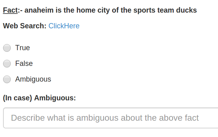
Figure 4: Sample BET posted to Mechanical turk for evaluating (ducks, homeCity, anaheim) belief edge in KG. (see Section 4.1)

To compare KGEval predictions against human evaluations, we evaluate all BETs $\{\mathcal{H}_{N}{}\cup\mathcal{H}_{Y}{}\}$ on AMT. For the ease of workers, we translate each entity-relation-entity belief into human readable format before posting to crowd. For instance, (Joe Louis Arena, homeStadiumOf, Red Wings) was rendered in BETs as “Stadium Joe Louis Arena is home stadium of sports team Red Wings” and asked to label true or false. To further capture strange cases of machine extractions, which might not make sense to an abstracted worker, we gave the option of classifying fact as ‘Ambiguous’ which later we disambiguated ourselves. Web search hyperlinks were provided to aid the workers in case they were not sure of the answer. Figure 4 shows a sample BET posted on AMT.

We published BETs on AMT under ‘classification project’ category. AMT platform suggests high quality Master-workers who have had a good performance record with classification tasks. We hired these AMT recognized master workers for high quality labels and paid $0.01 per BET. We correlated the labels of master workers and expert labels on 100 random beliefs and compared against three aggregated non-master workers. We observed that master labels were better correlated ($93\%$) as compared to non-masters ($89\%$), incurring one-third the cost. Consequently we consider votes of master workers for $\{\mathcal{H}_{N}{}\cup\mathcal{H}_{Y}{}\}$ as gold labels, which we would like our inference algorithm to be able to predict. As all BETs are of binary classification type, we consider uniform cost across BETs. Details are presented in Table 2.

Our focus, in this work, is not to address conventional problem of truth estimation from noisy crowd workers. We resort to simple majority voting technique in our analysis of noisy workers for structurally rich KG-Evaluation. For our experiments, we consider votes of master workers for $\{\mathcal{H}_{N}{}\cup\mathcal{H}_{Y}{}\}$ as gold labels, which we would like our inference algorithm to be able to predict. However, we also acknowledge several sophisticated techniques that have been proposed, like Bayesian approach, weighted majority voting etc., which are expected to perform better.

4.1.2 Performance Evaluation Metrics

Performance of various methods are evaluated using the following two metrics. To capture accuracy at the predicate level, we define $\Delta_{predicate}{}$ as the average of difference between gold and estimated accuracy of each of the $R$ predicates in KG.

$$\Delta_{predicate} = \frac{1}{|R|}\Bigg{(}\sum_{\forall r\in R}\Big{|}\Phi(\mathcal{H}{}_{r})-\frac{1}{|\mathcal{H{}}_{r}|}\sum_{\forall h\in\mathcal{H{}}_{r}}l(h)\Big{|}\Bigg{)}$$

We define $\Delta_{overall}{}$ as the difference between gold and estimated accuracy over the entire evaluation set.

$$\Delta_{overall} = \bigg{|}\Phi(\mathcal{H}{})-\frac{1}{|\mathcal{H}|}\sum_{\forall h\in\mathcal{H}}l(h)\bigg{|}$$

Above, $\Phi(\mathcal{H}{})$ is the overall gold accuracy, $\Phi(\mathcal{H}_{r}{})$ is the gold accuracy of predicate $r$ and $l(h)$ is the label assigned by the currently evaluated method. $\Delta_{overall}{}$ treats entire KG as a single bag of BETs whereas $\Delta_{predicate}{}$ segregates beliefs based on their type of predicate-relation. For both metrics, lower is better.

4.2 Baseline Methods

Since accuracy estimation of large multi-relational KGs is a relatively unexplored problem, there are no well established baselines for this task (apart from random sampling). We present below the baselines which we compared against KGEval.

Random: Randomly sample a BET $h\in\mathcal{H}$ without replacement and crowdsource for its correctness. Selection of every subsequent BET is independent of previous selections.

Max-Degree: Sort the BETs in decreasing order of their degrees in ECG and select them from top for evaluation; this method favors selection of more centrally connected BETs first.

Note that there is no notion of inferable set in the above two baselines. Individual BETs are chosen and their evaluations are singularly added to compute the accuracy of KG.

Independent Cascade: This method is based on contagion transmission model where nodes only infect their immediate neighbors [16]. At every time iteration $t$, we choose a BET which is not evaluated yet, crowdsource for its label and let it propagate its evaluation label in ECG.

KGEval: Method proposed in Algorithm 1.

4.3 Effectiveness of KGEval

NELL sports dataset ($\mathcal{H}_{N}$)
Method	$\Delta_{predicate}$	$\Delta_{overall}$	# Queries
	$(\%)$	$(\%)$
Random	$4.9$	$1.3$	623
Max-Deg	$7.7$	$2.9$	1370
Ind-Casc	$9.8$	$0.8$	232
KGEval	3.6	0.5	140
Yago dataset ($\mathcal{H}_{Y}$)
Random	$1.3$	$0.3$	513
Max-Deg	$1.7$	$0.5$	550
Ind-Casc	$1.1$	$0.7$	649
KGEval	0.7	0.1	204

Table 3: $\Delta_{predicate}(\%)$ and $\Delta_{overall}(\%)$ estimates (lower is better) of various methods with number of crowd-evaluated queries (BET evaluations) to reach the $\Delta_{overall}{}$ converged estimate. KGEval uses the least number of BET evaluations while achieving best estimates. This is our main result. (See Section 4.3)

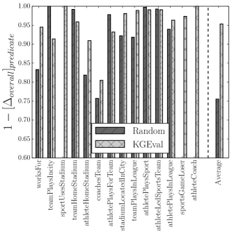
Figure 5: Comparing $(1-[\Delta_{overall}{}]_{predicate})$ of individual predicates (higher is better) in $\mathcal{H}_{N}$ between KGEval and Random, the two top performing systems in Table 3. $[\Delta_{overall}{}]_{predicate}$ means $\Delta_{overall}{}$ computed over beliefs of individual predicates. We observe that KGEval significantly outperforms Random in this task. (see Section 4.3)

Experimental results of all methods comparing $\Delta_{overall}{}$ at convergence (see Section 3.5 for definition of convergence), number of crowd-evaluated queries needed to reach convergence, and $\Delta_{predicate}{}$ at that convergence point are presented in Table 3. For both metrics, lower is better. From this table, we observe that KGEval, the proposed method, is able to achieve the best estimate across both datasets and metrics. This clearly demonstrates KGEval’s effectiveness. Due to the significant positive bias in $\mathcal{H}_{Y}{}$ (see Table 2), all methods do fairly well as per $\Delta_{overall}{}$ on this dataset, even though KGEval still outperforms others.

From this table, we also observe that KGEval is able to estimate KG accuracy most accurately while utilizing least number of crowd-evaluated queries. This clearly demonstrates KGEval’s effectiveness. We note that Random is the second most effective method.

Predicate-level Analysis

For this analysis we consider the top two systems from Table 3, viz., Random and KGEval, and compare performance on the $\mathcal{H}_{N}$ dataset. We use $(1-[\Delta_{overall}{}]_{predicate})$ as the metric (higher is better), where $[\Delta_{overall}{}]_{predicate}$ means $\Delta_{overall}{}$ computed over beliefs of individual predicates. Here, we are interested in evaluating how well the two methods have estimated per-predicate accuracy when KGEval’s $\Delta_{overall}{}$ has converged, i.e., after each method has already evaluated 140 queries (see $6^{th}$ row in Table 3). Experimental results comparing per-predicate performances of the two methods are shown in Figure 5. From this figure, we observe that KGEval significantly outperforms Random. KGEval’s advantage lies in its exploitation of coupling constraints among beliefs, where evaluating a belief from certain predicate helps infer beliefs from other predicates. As Random ignores all such dependencies, it results in poor estimates even at the same level of evaluation feedback.

4.4 Effectiveness of Coupling Constraints

Constraint Set	Iterations to	$\Delta_{overall}(\%)$
	Convergence
$\mathcal{C}{}$	140	0.5
$\mathcal{C}{}-\mathcal{C}{}_{b3}$	$259$	$0.9$
$\mathcal{C}{}-\mathcal{C}{}_{b3}-\mathcal{C}{}_{b2}$	$335$	$1.1$

Table 4: Performance of KGEval with ablated constraint sets. Additional constraints help in better estimation with lesser iterations.(see Section 4.4)

This paper is largely motivated by the thesis – exploiting richer relational couplings among BETs may result in faster and more accurate evaluations. To evaluate this thesis, we successively ablated Horn clause coupling constraints of body-length 2 and 3 from $\mathcal{C}_{N}{}$.

We observe that with the full (non-ablated) constraint set $\mathcal{C}_{N}{}$, KGEval takes least number of crowd evaluations of BETs to convergence, while providing best accuracy estimate. Whereas with ablated constraint sets, KGEval takes up to $2.4$x more crowd-evaluation queries for convergence. These results validate our thesis that exploiting relational constraints among BETs leads to effective accuracy estimation.

4.5 Additional Experiments

Unless otherwise stated, we perform experiments in this section over $\mathcal{H}_{N}$ using $\Delta_{overall}$ on convergence.

Effectiveness of KGEval’s Control Mechanism

We note that Random and Max-degree may be considered control-only mechanisms as they don’t involve any additional inference step. In order to evaluate how these methods may perform in conjunction with a fixed inference mechanism, we replaced KGEval’s greedy control mechanism in Line 5 of Algorithm 1 with these two control mechanism variants. We shall refer to the resulting systems as Random+inference and Max-degree+inference, respectively.

First, we observe that both Random + inference and Max-degree + inference are able to estimate accuracy more accurately than their control-only variants. Secondly, even though the accuracies estimated by Random+inference and Max-degree+inference were comparable to that of KGEval, they required significantly larger number of crowd-evaluation queries – $1.2$x and $1.35$x more, respectively. This demonstrates KGEval’s effective greedy control mechanism.

Rate of Coverage

Figure 6: Fraction of total beliefs whose evaluation where automatically inferred by different methods for varying number of crowd-evaluated queries (x-axis) in $\mathcal{H}_{N}$. KGEval automatically evaluates the largest number of BETs at each level (see Section 4.5).

Figure 6 shows the fraction of total beliefs whose evaluations were automatically inferred by different methods as a function of number of crowd-evaluated beliefs. We observe that KGEval infers evaluation for the largest number of BETs at each supervision level. Such fast coverage with lower number of crowdsource queries is particularly desirable in case of large KGs with scarce budget.

Robustness to Noise

In order to test robustness of the methods in estimating accuracies of KGs with different gold accuracies, we artificially added noise to $\mathcal{H}_{N}$ by flipping a fixed fraction of edges, otherwise following the same evaluation procedure as in Section 3.5. We chose triples which were evaluated to be true by crowd workers and also had functional predicate-relation to ensure that the artificially generated beliefs were indeed false. This resulted in variants of $\mathcal{H}_{N}$ with gold accuracies in the range of $81.3\%$ to $91.3\%$. We analyze $\Delta_{overall}{}$ (and not $\Delta_{predicate}{}$) because flipping edges in KG distorts predicate-relations dependencies.

We evaluated all the methods and observed that while performance of other methods degraded significantly with diminishing KG quality (more noise), KGEval was significantly robust to noise. Across baselines KGEval best estimated $\Delta_{overall}=0.8\%$ with $156$ BETs, whereas the next best baseline took $370$ BETs to give $\Delta_{overall}=1.2\%$. This along with KGEval’s performance on Yago2, a KG with naturally high gold accuracy, suggests that KGEval is capable of successfully estimating accuracies of KGs with wide variation in quality (gold accuracy).

4.6 Scalability and Run-time

Scalability comparisons with MLN

Markov Logic Networks (MLN) [29] is a probabilistic logic which can serve as another candidate for our Inference Mechanism. In order to compare the runtime performance of KGEval with PSL and MLN as inference engines, respective; we experimented with a subset of the NELL dataset with 1860 BETs and 130 constraints. We compared the runtime performance of KGEval with PSL and MLN as inference engines. While PSL took 320 seconds to complete one iteration, the MLN implementation could not finish grounding the rules even after 7 hours. This justifies our choice of PSL as the inference engine for KGEval.

Parallelism

Computing $\mathcal{I}(G,\mathcal{Q})$ for varying $\mathcal{Q}$ involves solving independent optimization function. The greedy step, which is also the most computationally intensive step, can easily be parallelized by distributing calculation of $\mathcal{I}(G,\mathcal{Q}\cup h_{i})$ among $i$ different computing nodes. The final aggregator node selects $\operatorname*{arg\,max}_{i}|\mathcal{I}(G,\mathcal{Q}\cup h_{i})|$.

Computational Optimization

Grounding of all first-order logic rules and maximizing their posterior probabilities, as in Equation (3), is computationally expensive. PSL inference engine uses Java implementation of hinge-loss Markov random fields (hl-mrf) to find the most probable explanation[3]. It also uses relational database for efficient retrieval during rule grounding [6].

5 Related Work

Most of the previous work on evaluation of large scale KGs has resorted to random sampling, whereas crowdsourcing research has typically considered atomic allocation of tasks wherein the requester posted Human Intelligence Tasks (HITs) independently. In estimating the accuracy of knowledge bases through crowdsourcing, we find the task of knowledge corroboration [15] to be closely aligned with our motivations. This work proposes probabilistic model to utilize a fixed set of basic first-order logic rules for label propagation. However, unlike KGEval, it does not look into the budget feasibility aspect and does not try to reduce upon the number of queries to crowdsource.

Most of the other research efforts along this line have gone into modeling individual workers and minimizing their required redundancy. They are mainly focused on getting a better hold on user’s behavior and use it to further get better estimates of gold truth [36]. Recent improvements use Bayesian techniques [13, 31] for predicting accuracy of classification type HITs, but they operate in much simpler atomic setting. None of them relate the outputs of HITs to one another and do not capture the relational complexities of our KG-Evaluation.

There have been models named Find-Fix-Verify which break large complex tasks, such as editing erroneous text, into modular chunks of simpler HITs and deal with these three inter-dependent tasks [4, 14]. The kind of inter-dependency among the three micro-tasks is very specific in the sense that output of previous stage goes as input to the next stage and cost analysis, workers Allocation and performance bounds over this model are done [34]. Our model transcends this restrictive linear dependence and is more flexible/natural. Decision theoretic approaches on constrained workflows have been employed to obtain high quality output for minimum allocated resources [18, 5]. Crowdsourcing tasks, like collective itinerary planning [37, 22], involves handling tasks with global constraints, but our notion of inter-dependence is again very different as compared to above model More recent work on construction of hierarchy over domain concepts [33], top-k querying over noisy crowd data [1], multi-label image annotation from crowd [9, 7] involve crowdsourcing over dependent HITs but their goals and methods vary largely from ours.

Our model significantly differs from previous works in marketing theory [11], outbreak detection [21] and social network analysis [16] etc., as it operates over multi-relational modes of inference and not just singular way of connecting two entities.

Work on budget sensitive algorithm [14, 2, 35] provides performance guarantees over several cost models, but do not account for any inter-relation among tasks.

In large scale crowdsourcing, recent works have highlighted case for active learning [26]. However, unlike our selection based on relational dependence at instance level tasks, active learning selection is based upon ranking generated over classifiers.

6 Conclusion

In this paper, we have initiated a systematic exploration into the important yet relatively unexplored problem of accuracy estimation of automatically constructed Knowledge Graphs (KGs). We have proposed KGEval, a novel method for this problem. KGEval is an instance of a novel crowdsourcing paradigm where dependencies among tasks presented to humans (belief evaluation in the current paper) are exploited. To the best of our knowledge, this is the first method of its kind. We demonstrated that the objective optimized by KGEval is in fact NP-Hard and submodular, and hence allows for the application of simple greedy algorithms with guarantees. Through extensive experiments on real datasets, we demonstrated effectiveness of KGEval.

As part of future work, we hope to extend KGEval to incorporate varying evaluation cost, and also explore more sophisticated evaluation aggregation.

Appendix A Appendix

Proof.

(for Theorem 1) The additional utility, in terms of label inference, obtained by adding a BET to larger set is lesser than adding it to any smaller subset. By construction, any two BETs which share a common factor node $\mathcal{C}{}_{j}$ are encouraged to have similar labels in $G$.

Potential functions $\psi_{j}$ of Equation (3) satisfy pairwise regularity property i.e., for all BETs $\{p,q\}\in\mathcal{H}{}$

$$\psi(0,1)+\psi(1,0)\geq\psi(0,0)+\psi(1,1)$$ (4)

where $\{1,0\}$ represent true/false. Equivalence of submodular and regular properties are established [17, 12]. Using non-negative summation property [23], $\sum_{j\in\mathcal{C}{}}\theta_{j}\psi_{j}$ is submodular for positive weights $\theta_{j}\geq 0$.

We consider a BET $h$ to be confidently inferred when the soft score of its label assignment in $\mathcal{I}(G,\mathcal{Q})$ is greater than threshold $\tau_{h}\in[0,1]$. From above we know that $\mathbb{P}(l(h)|\mathcal{Q})$ is submodular with respect to fixed initial set $\mathcal{Q}$. Although $\max$ or $\min$ of submodular functions are not submodular in general, but [16] conjectured that global function of Equation (1) is submodular if local threshold function $\mathbb{P}(h|\mathcal{Q})\geq\tau_{h}$ respected submodularity, which holds good in our case of Equation (3). This conjecture was further proved in [25] and thus making our global optimization function of Equation (1) submodular.

Proof.

(for Theorem 2) We reduce KGEval to NP-complete Set-cover Problem (SCP) so as to select $\mathcal{Q}$ which covers ${\mathcal{I}}(G,\mathcal{Q})$. For the proof to remain consistent with earlier notations, we define SCP by collection of subsets $\mathcal{I}_{1}{},\mathcal{I}_{2}{},\ldots,\mathcal{I}_{m}{}$ from set $\mathcal{H}{}=\{h_{1},h_{2},\ldots,h_{n}\}$ and we want to determine if there exist $k$ subsets whose union equals $\mathcal{H}{}$. We define a bipartite graph with $m+n$ nodes corresponding to $\mathcal{I}_{i}{}$’s and $h_{j}$’s respectively and construct edge $(\mathcal{I}_{i}{},h_{j})$ if $h_{j}\in\mathcal{I}_{i}{}$. We need to find a set $\mathcal{Q}$, with cardinality k, such that $|\mathcal{I}(G,\mathcal{Q})|\geq n+k$.

Choosing our BET-set $\mathcal{Q}$ from SCP solution and further inferring evaluations of other remaining BETs using PSL will solve the problem in hand.

A.1 Noisy Crowd Workers and Budget

Here, we provide a scheme to allot crowd workers so as to remain within specified budget and upper bound total error on accuracy estimate. We have not integrated this mechanism with Algorithm 1 to maintain its simplicity.

We resort to majority voting in our analysis and assume that crowd workers are not adversarial. So expectation over responses $r_{h}(u)$ for a task $h$ with respect to multiple workers $u$ is close to its true label $t(h)$ [35], i.e.,

$$\bigg{|}\mathbb{E}_{u\sim\mathbb{D}(u,h)}[r_{h}(u)]-t{(h)}\bigg{|}\leq\frac{1}{2}$$ (5)

where $\mathbb{D}$ is joint probability distribution of workers $u$ and tasks $h$.

Our key idea is that we want to be more confident about BETs $h$ with larger inferable set (as they impact larger parts of KG) and hence allocate them more budget to post to more workers. We determine the number of workers $\{w_{h_{1}},\ldots,w_{h_{n}}\}$ for each task such that $h_{t}$ with larger inference set have higher $w_{h_{t}}$. For total budget $B$, we allocate

$w_{h_{t}}=\big{\lfloor}\frac{B~{}i_{t}~{}(1-\gamma)}{c~{}i_{max}}\big{\rfloor}$

where $i_{t}$ denotes the cardinality of inferable set $\mathcal{I}(G,\mathcal{Q}\cup h_{t})$, $c$ the cost of querying crowd worker, $i_{max}$ the size of largest inferable set and $\gamma\in[0,1]$ constant.

This allocation mechanism easily integrates with Algorithm 1; in (Line 8) we determine size of inferable set $i_{t}=|\mathcal{Q}_{t}|$ for task $h$ and allocate $w_{h}$ crowd workers. Budget depletion (Line 9) is modified to $B_{r}=B_{r}-w_{h}c(h)$. The following theorem bounds the error with such allocation scheme.

Theorem 1.

[Error bounds] The allocation scheme of redundantly posing $h_{t}$ to $w_{h_{t}}$ workers does not exceed the total budget $B$ and its expected estimation error is upper bounded by $e^{-O(i_{t})}$, keeping other parameters fixed. The expected estimation error over all tasks is upper bounded by $e^{-O(B)}$.

Proof.

Let $\gamma\in[0,1]$ control the reduction in size of inferable set by $i_{t+1}=\gamma~{}i_{t}$. By allocating $w_{h_{t}}$ redundant workers for task $h_{t},\forall t\in\{1\cdots n\}$ with size of inferable set $i_{t}$, we incur total cost of

$$\sum_{t=1}^{n}c~{}w_{h_{t}} = \sum_{t=1}^{n}\frac{B~{}i_{t}~{}(1-\gamma)}{c~{}i_{max}}\cdot c$$

$$= \left(\sum_{t=1}^{n}i_{t}\right)\cdot\left(\frac{B~{}(1-\gamma)}{i_{max}}\right)$$

For greedy control mechanism, $i_{1}=i_{max}$. Suppose we approximate the reduction in size of inferable set by a diminishing factor of $\gamma\in(0,1)$ i.e $i_{t+1}=\gamma~{}i_{t}$.

$$= \left(\frac{i_{max}~{}(1-\gamma^{T})}{(1-\gamma)}\right)\cdot\left(\frac{B~{}(1-\gamma)}{i_{max}}\right)$$

$$\leq B$$

Note that the above geometric approximation, which practically holds true when decaying is averaged over few time steps, helps in getting an estimate of $\sum_{t=1}^{T}i_{t}$ at iteration $t\leq T$. Such approximation would not be possible unless we already ran the entire experiment. For practical implementation, we can use an educated guess of $\gamma=1-\frac{i_{max}}{\mathrm{avg}_{t}(i_{t})}$.

Error Bounds: Here we show that the expected error of estimating of $h_{t}$ for any time $t$ decreases exponentially in the size of inferable set $i_{t}$. We use majority voting to aggregate $w_{h_{t}}$ worker responses for $h_{t}$, denoted by $\hat{r}_{h_{t}}\in\{0,1\}$

$$\hat{r}_{h_{t}}=\Bigg{\lfloor}\frac{1}{w_{h_{t}}}\sum_{k=1}^{w_{h_{t}}}r_{h_{t}}(u_{k})-\frac{1}{2}\Bigg{\rfloor}+1$$ (6)

where $r_{h_{t}}(u_{k})$ is the response by $k^{th}$ worker for $h_{t}$. The error from aggregated response can be given by $\Delta({h_{t}})=|\hat{r}_{h_{t}}-t(h_{t})|$, where $t(h_{t})$ is its true label. From Equation (5) and Hoeffding-Azuma bounds over $w_{h_{t}}$ i.i.d responses and error margin $\varepsilon_{t}$, we have

$$\Delta({h_{t}}) = \mathbb{P}\Bigg{\{}\Bigg{|}\frac{1}{w_{h_{t}}}\sum_{k=1}^{w_{h_{t}}}r_{h_{t}}(u_{k})-\mathbb{E}(r_{h}(u))\Bigg{|}\geq\varepsilon_{t}\Bigg{\}}$$

$$\leq 2e^{-2w_{h_{t}}\varepsilon_{t}^{2}}$$

$$= 2~{}\mathrm{exp}\left(-2~{}\frac{B~{}i_{t}~{}(1-\gamma)}{c~{}i_{max}}~{}\varepsilon_{t}^{2}\right)$$

For fixed budget $B$ and given error margin $\varepsilon_{t}$, we have $\Delta({h_{t}})=e^{-O(i_{t})}$. Summing up over all tasks $t$, by union bounds we get the total expected error from absolute truth as $\Delta(B)=\sum_{t=1}^{n}\Delta({h_{t}})$.

$$\Delta(B) \leq \sum_{t=1}^{n}2~{}\mathrm{exp}\left(-2~{}\frac{B~{}i_{t}~{}(1-\gamma)}{c~{}i_{max}}~{}\varepsilon_{t}^{2}\right)$$

$$\leq n\cdot 2~{}\mathrm{exp}\left(-2~{}\frac{B~{}i_{min}~{}(1-\gamma)}{c~{}i_{max}}~{}\varepsilon_{min}^{2}\right)$$

The accuracy estimation error will decay exponentially with increase in total budget for fixed parameters.

References

- [1] A. Amarilli, Y. Amsterdamer, T. Milo, and P. Senellart. Top-k querying of unknown values under order constraints, 2015.
- [2] A. Azaria, Y. Aumann, and S. Kraus. Automated strategies for determining rewards for human work. In AAAI. Citeseer, 2012.
- [3] S. H. Bach, B. Huang, B. London, and L. Getoor. Hinge-loss Markov random fields: Convex inference for structured prediction. In UAI, 2013.
- [4] M. S. Bernstein, G. Little, R. C. Miller, B. Hartmann, M. S. Ackerman, D. R. Karger, D. Crowell, and K. Panovich. Soylent: a word processor with a crowd inside. In ACM symposium on User interface software and technology, pages 313–322, 2010.
- [5] J. Bragg, D. S. Weld, et al. Crowdsourcing multi-label classification for taxonomy creation. In HCOMP, 2013.
- [6] M. Broecheler, L. Mihalkova, and L. Getoor. Probabilistic similarity logic. In UAI, 2010.
- [7] J. Deng, O. Russakovsky, J. Krause, M. S. Bernstein, A. Berg, and L. Fei-Fei. Scalable multi-label annotation. In SIGCHI, pages 3099–3102, 2014.
- [8] X. Dong, E. Gabrilovich, G. Heitz, W. Horn, N. Lao, K. Murphy, T. Strohmann, S. Sun, and W. Zhang. Knowledge vault: A web-scale approach to probabilistic knowledge fusion. In SIGKDD, pages 601–610, 2014.
- [9] L. Duan, S. Oyama, H. Sato, and M. Kurihara. Separate or joint? estimation of multiple labels from crowdsourced annotations. Expert Systems with Applications, 41(13):5723–5732, 2014.
- [10] L. A. Galárraga, C. Teflioudi, K. Hose, and F. Suchanek. Amie: association rule mining under incomplete evidence in ontological knowledge bases. In WWW, pages 413–422, 2013.
- [11] J. Goldenberg, B. Libai, and E. Muller. Using complex systems analysis to advance marketing theory development: Modeling heterogeneity effects on new product growth through stochastic cellular automata. Academy of Marketing Science Review, 9(3):1–18, 2001.
- [12] S. Jegelka and J. Bilmes. Submodularity beyond submodular energies: coupling edges in graph cuts. In CVPR, pages 1897–1904, 2011.
- [13] E. Kamar, S. Hacker, and E. Horvitz. Combining human and machine intelligence in large-scale crowdsourcing. In AAMAS, pages 467–474, 2012.
- [14] D. R. Karger, S. Oh, and D. Shah. Budget-optimal task allocation for reliable crowdsourcing systems. Operations Research, 62(1):1–24, 2014.
- [15] G. Kasneci, J. Van Gael, R. Herbrich, and T. Graepel. Bayesian knowledge corroboration with logical rules and user feedback. In Machine Learning and Knowledge Discovery in Databases, pages 1–18. 2010.
- [16] D. Kempe, J. Kleinberg, and É. Tardos. Maximizing the spread of influence through a social network. In SIGKDD, 2003.
- [17] V. Kolmogorov and R. Zabih. What energy functions can be minimized via graph cuts? Pattern Analysis and Machine Intelligence, IEEE Transactions on, 26(2):147–159, 2004.
- [18] A. Kolobov, D. S. Weld, et al. Joint crowdsourcing of multiple tasks. In HCOMP, 2013.
- [19] F. R. Kschischang, B. J. Frey, and H.-A. Loeliger. Factor graphs and the sum-product algorithm. Information Theory, IEEE Transactions on, 47(2):498–519, 2001.
- [20] N. Lao, T. Mitchell, and W. W. Cohen. Random walk inference and learning in a large scale knowledge base. In EMNLP, pages 529–539, 2011.
- [21] J. Leskovec, A. Krause, C. Guestrin, C. Faloutsos, J. VanBriesen, and N. Glance. Cost-effective outbreak detection in networks. In SIGKDD, pages 420–429, 2007.
- [22] G. Little, L. B. Chilton, M. Goldman, and R. C. Miller. Turkit: human computation algorithms on mechanical turk. In Proceedings of the 23nd annual ACM symposium on User interface software and technology, pages 57–66. ACM, 2010.
- [23] L. Lovász. Submodular functions and convexity. In Mathematical Programming The State of the Art, pages 235–257. Springer, 1983.
- [24] T. Mitchell, W. Cohen, E. Hruschka, P. Talukdar, J. Betteridge, A. Carlson, B. Dalvi, M. Gardner, B. Kisiel, J. Krishnamurthy, N. Lao, K. Mazaitis, T. Mohamed, N. Nakashole, E. Platanios, A. Ritter, M. Samadi, B. Settles, R. Wang, D. Wijaya, A. Gupta, X. Chen, A. Saparov, M. Greaves, and J. Welling. Never-ending learning. In Proceedings of AAAI, 2015.
- [25] E. Mossel and S. Roch. On the submodularity of influence in social networks. In ACM symposium on Theory of computing, pages 128–134, 2007.
- [26] B. Mozafari, P. Sarkar, M. Franklin, M. Jordan, and S. Madden. Scaling up crowd-sourcing to very large datasets: a case for active learning. VLDB, 8(2):125–136, 2014.
- [27] G. L. Nemhauser, L. A. Wolsey, and M. L. Fisher. An analysis of approximations for maximizing submodular set functions—i. Mathematical Programming, 14(1):265–294, 1978.
- [28] J. Pujara, H. Miao, L. Getoor, and W. Cohen. Knowledge graph identification. In The Semantic Web–ISWC 2013, pages 542–557. Springer, 2013.
- [29] M. Richardson and P. Domingos. Markov logic networks. Machine learning, 62(1-2):107–136, 2006.
- [30] M. Samadi, P. Talukdar, M. Veloso, and T. Mitchell. Askworld: budget-sensitive query evaluation for knowledge-on-demand. In Proceedings of the 24th International Conference on Artificial Intelligence, pages 837–843. AAAI Press, 2015.
- [31] E. Simpson, S. J. Roberts, A. Smith, and C. Lintott. Bayesian combination of multiple, imperfect classifiers. 2011.
- [32] F. M. Suchanek, G. Kasneci, and G. Weikum. Yago: a core of semantic knowledge. In WWW, 2007.
- [33] Y. Sun, A. Singla, D. Fox, and A. Krause. Building hierarchies of concepts via crowdsourcing. arXiv preprint arXiv:1504.07302, 2015.
- [34] L. Tran-Thanh, T. D. Huynh, A. Rosenfeld, S. D. Ramchurn, and N. R. Jennings. Budgetfix: budget limited crowdsourcing for interdependent task allocation with quality guarantees. In AAMAS, pages 477–484, 2014.
- [35] L. Tran-Thanh, M. Venanzi, A. Rogers, and N. R. Jennings. Efficient budget allocation with accuracy guarantees for crowdsourcing classification tasks. In AAMAS, 2013.
- [36] P. Welinder, S. Branson, P. Perona, and S. J. Belongie. The multidimensional wisdom of crowds. In NIPS, pages 2424–2432, 2010.
- [37] H. Zhang, E. Law, R. Miller, K. Gajos, D. Parkes, and E. Horvitz. Human computation tasks with global constraints. In SIGCHI, pages 217–226, 2012.