Observations of the Formation, Development, and Structure of a Current Sheet in an Eruptive Solar Flare

Abstract

We present AIA observations of a structure we interpret as a current sheet associated with an X4.9 flare and coronal mass ejection that occurred on 2014 February 25 in NOAA Active Region 11990. We characterize the properties of the current sheet, finding that the sheet remains on the order of a few thousand km thick for much of the duration of the event and that its temperature generally ranged between 8–10 MK. We also note the presence of other phenomena believed to be associated with magnetic reconnection in current sheets, including supra-arcade downflows and shrinking loops. We estimate that the rate of reconnection during the event was $M_{A}\approx$ 0.004–0.007, a value consistent with model predictions. We conclude with a discussion of the implications of this event for reconnection-based eruption models.

1 Introduction

Magnetic reconnection, the topological restructuring of magnetic field lines embedded in a highly conducting plasma, is widely accepted to be the mechanism that converts stored magnetic energy into heat and kinetic energy during eruptive solar flares. In the standard model (Kopp & Pneuman, 1976) a current sheet forms between antiparallel field lines that are stretched outwards from the Sun in the wake of an eruption. Reconnection in this current sheet releases magnetic energy that powers a solar flare and simultaneously reconfigures the field to form the post-flare loops and flare ribbons commonly associated with these types of eruptive events (Forbes et al., 1989).

Reconnection-based flare models can explain a wide variety of phenomena that are observed in association with eruptive flare current sheets, including shrinking loops (Forbes & Acton, 1996; Reeves et al., 2008) and inflows in the vicinity of flares (McKenzie & Hudson, 1999; McKenzie & Savage, 2009). Reconnection models, meanwhile, have been refined since Kopp & Pneuman’s seminal paper, and capture the dynamics and phenomena associated with these events with ever-improving accuracy (see, for example, Lin & Forbes, 2000). There are numerous reports of observations of reconnection-related phenomena in the literature, many of which are discussed below. However, there is still a need for direct observational confirmation of predictions from theory and numerical models, many of which remain poorly constrained. There is a particular need for observations that can help constrain properties of reconnection itself and, in turn, help us understand more precisely how reconnection liberates stored magnetic energy during eruptions.

Of special importance are observations that can put limits on the reconnection rate, which is a free parameter in many models. The indeterminacy in reconnection models is discussed in detail by Forbes et al. (2013), who point out that the Petschek model for reconnection, which itself is at the heart of many reconnection-based eruption models, does not make a specific prediction of the reconnection rate. So the need for observational constraints is acute.

Likewise, other aspects of models can also be constrained by observation. Yokoyama & Shibata (1997), Yokoyama & Shibata (2001), and Seaton & Forbes (2009) all discuss the role of thermal conduction in the energetics of reconnection in eruptive flares, but there have been few observations that might allow us to assess how much conduction actually influences the evolution of reconnection in eruptive events. This in spite of the fact that new models are being developed that take such effects into account (Scott et al., 2013).

Cusp-shaped structures that form in the wake of solar flares are now widely understood to be important evidence of reconnection as well. This realization is present in the earliest discussions of such a model (Kopp & Pneuman, 1976) and there are now numerous reports of such structures in observations during solar flares and eruptions that can be associated with both reconnection and current sheets. (See Gou et al. 2015 for one such example; for an extensive list of such observations, see Table 2 in Lin et al. 2015.)

There are also reports of observations of flare-associated current sheets and related phenomena using a variety of instruments and wavelengths. These range from detections in hard x-rays (Susino et al., 2013) using the Reuven Ramaty High-Energy Solar Spectroscopic Imager (RHESSI; Lin et al., 2002) to radio wavelengths (Aurass et al., 2013). In fact, the list of such observations is far too long to discuss in any detail in this short introduction; for a much more complete overview readers may wish to consult Lin et al. (2015), who discuss many other observations of current sheets, the properties of the observed sheets, and other associated phenomena.

Here we focus on several specific observations that, like the one we report in this paper, showed direct evidence of the current sheet itself and provided the opportunity to test predictions by flare reconnection models or to infer parameters that could be used to constrain those models.

Before we continue, it is worth pointing out that there is not a consensus on what the size of a current sheet in the solar corona is likely to be; predictions range from Larmor-radius scales of just a few meters to megameters. Nor for that matter, is there consensus on whether current sheets can actually be identified observationally and separated from other related, larger-scale structures Different authors have dealt with this observational ambiguity in different ways, and correspondingly have referred to structures in their observations that might be related to current sheets with a variety of terminology. In this paper we will adopt a simple convention: we refer to the entirety of the spine-like structure in our extreme-ultraviolet (EUV) observations simply as the “current sheet”, and our use of this term throughout the paper more generally refers to long, narrow structures on megameter scales that have been identified observationally by a variety of authors.

For example, Reeves & Golub (2011) reported observations from the Atmospheric Imaging Assembly (AIA; Lemen et al., 2012) on NASA’s Solar Dynamics Observatory (SDO; Pesnell et al., 2012) of high temperature reconnection-related plasma during an off-limb eruptive flare that occurred on 2010 November 3. Later analysis by Cheng et al. (2011) and Savage et al. (2012a) provided further support to this hypothesis.

One of the clearest observations of a current sheet was reported by Savage et al. (2010), who described a very narrow structure above a post-flare arcade system in observations from the X-Ray Telescope (XRT; Golub et al., 2007) on-board the Hinode spacecraft following the so-called “Cartwheel CME” that occurred on 2008 April 9. These authors reported the width of this structure to be 4–5$\times 10^{3}\,\mathrm{km}$ and discussed its association with other phenomena — inflows and shrinking loops — that are believed to be signatures of magnetic reconnection associated with eruptive flares.

A more recent paper by Zhu et al. (2016) presented the analysis of a current sheet that formed during a C2.0 flare. Zhu et al. observed a hot, extended structure that formed at the top of cusp-shaped loops during the event and showed, like Savage et al., that the structure was associated with the type of inflows and outflows predicted by reconnection models. On the other hand, unlike the current sheet described in the report by Savage et al., this one was imaged in front of the solar disk instead of in profile on the limb. This perspective afforded Zhu et al. a good view of the conditions in the region at the onset of the event, from which they concluded that this current sheet — although fundamentally similar to the fast growing sheets observed during eruptive flares by other teams — was likely generated by a loop-loop interaction and may have grown considerably more slowly as a result.

There have also been reports of observations of suspected current sheets in white light images that provided similar opportunities to characterize important parameters. Ling et al. (2014) described observations from the ground-based Mk4 K-Coronameter at the Mauna Loa Solar Observatory (Elmore et al., 2003) in the wake of a CME on 2005 September 7. This eruption was associated with a flare that was classified at least X17 (the flare saturated the X-Ray Sensor on GOES, so its exact brightness is not known) and a CME with speeds in excess of 2500 km/s. These authors measured properties of the current sheet at considerably larger heights than the measurements reported by Savage et al. (2010), and found that the width of the current sheet was roughly $2\times 10^{4}\,\mathrm{km}$ out to heights as large as nearly 3 solar-radii.

In general, observations of current sheets such as these provide an opportunity to estimate the rate of magnetic reconnection during the event, which is usually reported in terms of the inflow Alfvén Mach number, $M_{A}$. $M_{A}$, in turn, is proportional both to the ratio of inflow to outflow velocities, $V_{in}/V_{out}$ and the ratio of width to length of the sheet, $l/L$ (see Priest & Forbes, 2000). Savage et al. (2010) used the second ratio, based on the geometric properties of the sheet they observed, to determine a reconnection rate between $0.002-0.006$, while Ling et al., using the same method, found values of $M_{A}$ closer to 0.07, a number more consistent with predictions from many models. Lin & Forbes (2000), for example, describe a model with $M_{A}=0.1$, though it is worth pointing out that they note a rate as low as $M_{A}=0.005$ can still yield an eruption. Zhu et al. measured the reconnection rate by estimating flow velocities and found $M_{A}$ between about 0.01 and 0.05.

The reconnection rate is an especially important property for constraining reconnection-based eruption models because it determines the rate at which magnetic energy can be converted to heat and kinetic energy to drive a solar eruption and flare. Exactly what determines rate of reconnection in the corona and, as we mentioned above, what the rate is predicted to be, remains the subject of much research and discussion (Forbes et al., 2013).

It is also worth noting that current sheets in the corona are complex, three-dimensional structures whose appearances are determined by many factors, especially the perspective from which they are observed. Accordingly, there have been many other reports of current-sheet-associated phenomena that do not fit the classical, two-dimensional cross-sectional picture. When viewed face-on, current sheets are often described as “fans” (see, for example, Khan et al., 2007; Savage & McKenzie, 2011; Warren et al., 2011). From this perspective, the current sheet is a broad, turbulent, high-temperature curtain punctuated by fast inflowing loops that often trail dark voids, commonly referred to as supra-arcade downflows (SADs) in their wake (Savage et al., 2012b). Observations of fans and inflows have been made using a variety of imagers — for example, the Yohkoh Soft X-Ray Telescope (McKenzie & Hudson, 1999), the Transition Region and Coronal Explorer (Gallagher et al., 2002), XRT Lin et al. (2015), and AIA (Savage et al., 2012b) — and have been believed to be linked to reconnection since their first detection during the Yohkoh mission nearly two decades ago. As we will discuss later in this paper, these manifestations are part and parcel of the same current sheet phenomena observed in this and other events. One peculiarity of the event we discuss in this paper is that the three-dimensional nature of the sheet provides the opportunity to study both edge-on and face-on phenomena simultaneously.

Observations of face-on phenomena like SADs, too, can provide an opportunity to evaluate model predictions. Hanneman & Reeves (2014), for example, used differential emission measure (DEM) analysis to characterize the temperature structure of a number of SADs and the surrounding plasma, and found that the current sheet plasma in the fans often had temperatures in excess of $10^{7}$ K, and SADs, while hot, were generally cooler than the surrounding fan.

Likewise, in an analysis of similar events Scott et al. (2016) attempted to deduce the magnetic structure of SADs and the plasma that surrounds them. In particular, they attempted to determine the plasma beta, which is the ratio between thermal and magnetic energy density in a plasma. Beta is an important parameter in reconnection models, and is often assumed to be very small, as it is in most of the low corona. Their analysis showed that this assumption is likely incorrect, providing another important constraint for theory and models.

In this paper we present AIA observations of an X4.9 flare that occurred on 2014 February 25 that contain evidence of the presence of an extended, high-temperature current sheet that formed in the wake of an eruption and was clearly associated with the growth of the post-flare loop system. We attempt to measure or detect several properties of the sheet structure that might be useful in constraining reconnection and eruption models, including the reconnection rate and the presence of a thermal halo that might be linked to conduction from the sheet into the surrounding corona. We also discuss its association with commonly observed eruptive flare-related phenomena like supra-arcade downflows and shrinking loops. We conclude with a few remarks about what can be learned from observations like these and how research into the nature of magnetic reconnection during solar eruptions might be enhanced by future instrumentation.

2 Observations

The structures we report on in this paper were formed in association with a large and complex filament eruption that occurred on the east limb of the Sun in NOAA Active Region 11990 at about 00:40 UT on 2014 February 25. This eruption was also associated with an impulsive X4.9 class flare, which peaked about 10 minutes after the onset of the eruption, and a very energetic CME with a reported velocity of more than 2100 km/s in the CDAW CME Catalog (for a description of CDAW, see Yashiro et al., 2004). X-ray irradiance measurements of the flare from the GOES spacecraft show a nearly instantaneous rise to the peak brightness from the onset of the event, and a long and gradual decay to background levels some 6–8 hours after the event’s onset. Figure 1 shows a plot of the measured irradiance during the event.

Figure 1: X-ray irradiance measured by the GOES X-Ray Sensor instrument, beginning at midnight on 2014 February 25. The black curve corresponds to the 1–8 Å channel while the gray curve shows the 0.5–4 Å channel.

A previous analysis of this event by Chen et al. (2014) presented evidence that the filament eruption itself was triggered by tether-cutting reconnection at the base of the erupting filament. These authors did not, however, examine the role that reconnection played in the development of structures that formed later in the event’s evolution.

In this paper we focus on a structure, which we interpret as the manifestation of a current sheet, that appeared only after the eruption’s onset and continued to evolve for at least six hours, throughout the decay phase of the flare. We studied this event using observations from the AIA and, although we used observations from all of AIA’s available extreme-ultraviolet channels, we focused in particular on observations in the 131 Å channel because its response to high-temperature Fe XXI (O’Dwyer et al., 2010) provided the best view of the current sheet structure that is the subject of this paper.

The feature of interest in this paper formed in the wake of the erupting filament that was visible in AIA images between 00:40 and 00:52. The structure first appears as a very narrow spine, growing outward from the flare site between 00:59 and 01:04. This structure remains very thin for nearly an hour, until about 01:40, when it begins to widen. By 1:47, a fainter cusp-shaped structure appears at the base of the spine, above the post-eruptive loops associated with the flare. The cusp broadens over time until it reaches its maximum width at around 03:40. Finally, the cusp structure narrows and becomes fainter over time, but remains distinct from the background until about 08:00, while the spine structure disappears progressively downwards into the cusp structure by about 05:50.

Figure 2 and the accompanying animation show the evolution of the flare region over the course of the event. To generate this sequence of images we first eliminated underexposed images generated by AIA’s automatic flare exposure control, which produces short-exposure images during bright flares. Although this exposure control helps to limit the amount of saturation and blooming due to the flare itself, the resulting images did not provide a good view of the current sheet structure.

Figure 2: The evolution of current sheet structure in the 131 Å AIA channel beginning with its appearance in the wake of a strong CME. Early on (upper left) the structure is long and narrow, and only later (upper right) do background features begin to appear. These features are first seen as shrinking loops, which later broaden (middle left, black arrow) into a more fan-like structure while the sheet itself (middle left, white arrow) begins to broaden. As the sheet broadens, shrinking loops are clearly visible in the cusp region at the current sheet’s base (middle right). Even later (lower left) dark inflows, presumably SADs, become visible in the diffuse background emission. At very late times (lower right) some material appears to flow into the sheet itself, triggering bifurcated up-down flows along the sheet structure. An animation of the evolution of this structure is included with the online version of this paper.

Many of the dynamic features of this event are the result of very weak variations in already faint signals, so we further processed these images to improve the visibility of these features and reduce noise. We began by median-stacking them in groups of seven, which appeared to yield the best balance between avoiding motion blur while controlling image noise. We then applied a routine included in the SolarSoft IDL (Freeland & Handy, 1998) branch for the SWAP instrument (Seaton et al., 2013b) on-board PROBA2 called gentle_filter.pro. This algorithm is a noise filter that suppresses individual pixels that are strong outliers compared to their neighbors without significantly reducing image sharpness; we applied it to the resulting images to further remove speckle noise in the images. Finally, we applied an image filter that improved local image contrast by normalizing the image brightness using a function derived from a gaussian-smoothed copy of the image. The resulting images were combined into a movie in which large-scale features are preserved while the visibility of local variations is enhanced.

The six different panels of Figure 2 highlight several important phenomena that we observed during the event. The first panel (top left) at 01:05, shows the early formation of the current sheet, which is highlighted by the white arrow. By 01:23 (top right) the current sheet structure is well-formed and there are indications of a coronal fan structure forming as well, indicated again by a white arrow. This fan is almost certainly related to the current sheet, but is seen face-on rather than edge-on thanks to the complicated three-dimensional nature of this event.

By 01:49, the time of the third panel (middle left) the bottom of the sheet has begun to broaden as described above (white arrow), while the fan has become much more visible and highly structured (black arrow). By 02:40 (middle right) we see many loops shrinking through the broad, cusp-shaped feature at the bottom of the sheet, a clear indication that flare-related reconnection is probably taking place.

Throughout this time we also see evidence of SADs in the fan both to the north and south of the sheet. The white arrow in the panel at 03:40 (bottom left) indicates one example of such an inflow. These inflows are another common phenomenon associated with flare reconnection, and are closely linked with the flows we see along the sheet itself. This is yet another indication that the fan and sheet are part of the same three-dimensional structure viewed at different angles.

By the time of the final panel (bottom right) at 05:23 there are indications not only of downflows from above, but also of flows into the current sheet itself. The white arrow highlights one such example, which appears to be advected into the sheet before bifurcating into upward- and downward-directed flows. This may be an indication of ongoing magnetic reconnection, or even of the presence of an magnetic neutral point or flow stagnation point in the sheet. Unfortunately, due to the weak contrast of these features, we could not make quantitative measurements of the nature of these flows. Because of this, and because of the highly turbulent nature of this region more generally, we hesitate to draw any strong conclusions about the fundamental nature of these flows.

3 Analysis

3.1 The structure of the current sheet

It is worth emphasizing once more the complex, three-dimensional nature of the structures associated with this eruption. From the perspective of SDO, we see post-eruptive loops both from the edge-on perspective, as in those highlighted in the panel of Figure 2 at 01:49 UT, and in a face-on perspective, like the shrinking loops that appear in the panel at 02:40. Here we focus our analysis on the spine-like current sheet structure that overlies the shrinking loops, because it provides a rare opportunity to deduce some of the properties of eruption-associated magnetic reconnection directly from observations.

However, the association of this feature with the more frequently observed SADs and coronal fan structure is also important. Although SADs and fans have long been understood to be the manifestation of current sheets viewed from the face-on perspective, there have been very few observations that clearly reveal both aspects of this phenomenon simultaneously. This event provides a unique opportunity for direct confirmation of the relationship between these phenomena.

The focus of our analysis here was to determine properties of the spine-like current sheet structure that might help us characterize the processes that underlie both the structure’s formation and the eruption itself. We measured the width of the sheetlike structure using a combination of algorithmic image processing and visual inspection. We first used an automated algorithm to determine the brightest point in every column the feature spanned. We then fit the resulting points using a piecewise-defined linear regression fit such that the changing slope of the feature over its length was well-captured by the fit.

We used the slope from the linear fit to define an intersecting sample of 100 pixels perpendicular to the feature. Because the thickness of the structure varied somewhat, we selected the location of the point of measurement with respect to each subframe to obtain a representative value for the thickness.

We sampled the background brightness by computing the mean of a small region of pixels near — but not including — the structure. We then iteratively rejected pixels which were not brighter than the background value times a constant, progressively increasing the constant until no background points remained that were clearly beyond the edge of the feature, as determined by visual inspection. We then computed the width of the feature at various points along its length by measuring the distance between between the first and last of the remaining points. We consider this measurement to be the upper limit on the width of the feature.

In many cases, however, the width of the feature is ambiguous, since its edges are poorly defined. We thus determined a lower limit on the width of the feature by increasing the background value further until the remaining points barely spanned the feature, as determined by visual inspection. Figure 3 shows an illustration of the approach we used to measure widths of the current sheet at various heights, the results are reported numerically in Table 1. The values of width reported in the table are the mean of the upper and lower limit for the various points at which we measured the feature, while the reported error is the mean of the difference between these limits and the reported width.

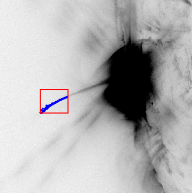
(a)

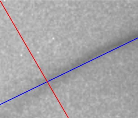
(b)

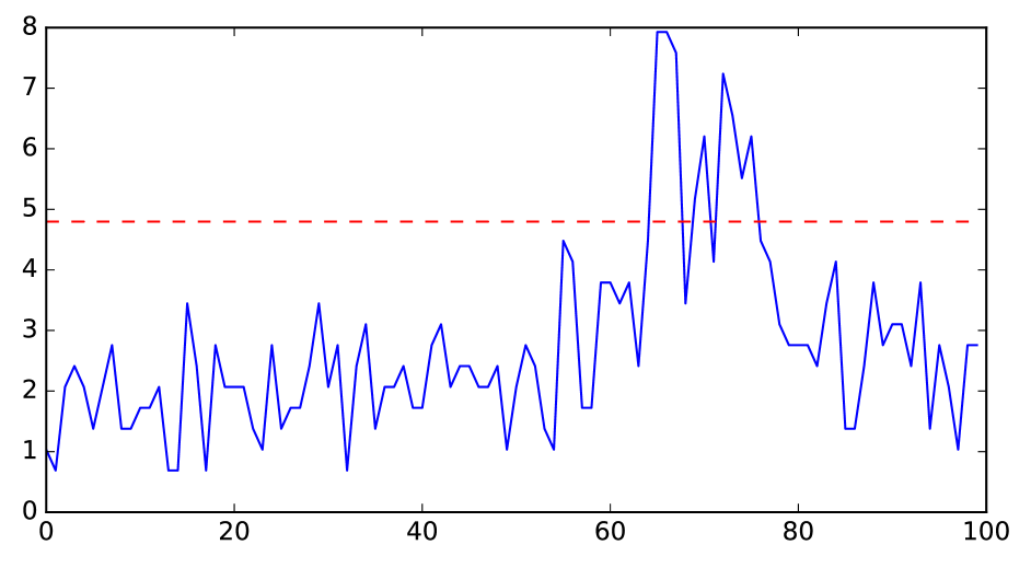
(c)

Figure 3: An illustrative overview of the method we used to measure current sheet widths. We first identified the location of the sheet in a sub-region by locating the brightest pixel in each column (upper left). We then fit these points with a line and sampled a cross-section of the current sheet feature perpendicular to this line (upper right). We identified the width by determining a background noise floor value above which the outermost edges of the feature were clearly part of the current sheet (bottom).

We generally considered the maximum width to be the widest possible measurement where no pixel clearly extended into the background, and the minimum to be the thinnest measurement that completely spanned the feature. For example, the base of the feature in the image from 03:20:44 has a cusp-like structure with the more or less uniform brightness, the width of which we considered to be the minimum, as well as a fainter extension of the cusp extending along the north side of the feature, which was included in the maximum.

We performed this measurement on images obtained at 1:20:20, 1:40:20, and 3:20:44. Figure 4 shows where width measurements were taken (indicated by arrows) throughout the evolution of the structure. The image from 00:10:08 shows the region before the eruption, and confirms there are few strong background features that might interfere with measurements in the later images. Although all of the images in the figure are displayed using a power-law scaling with a gamma of 0.4, the data used in our width measurements were not scaled. It is worth noting that the images at 1:40:20 and 3:20:44 were created by computing the median-value of pixels from a stack of three images: an image at the given time, an image immediately preceding the given time, and an image immediately following the given time, to help reduce detector-related noise.

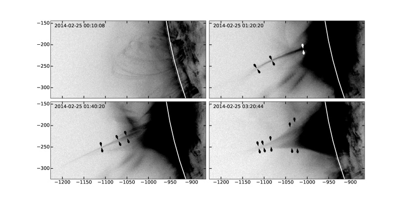
Figure 4: Measured widths of the current sheet at various times and locations during its evolution. The panel in the upper left, at 00:10:08 UT, from before the eruption onset, is included to show that there is relatively little pre-existing background structure that might influence our ability to accurately measure the sheet width later on.

Table 1: Measured current sheet width and error at various heights and times in the evolution of the event.

	Height (solar-radii)	Width (km)	Error (km)
01:20:20	1.181	3880	860
	1.142	1720	430
	1.064	2800	220
01:40:20	1.173	1720	430
	1.129	3280	950
	1.108	4840	1560
03:20:44	1.177	3980	1360
	1.165	4710	400
	1.146	10200	640
	1.098	31800	4100
	1.083	38300	6290

At this point is is worthwhile to ask whether these measurements are really likely to provide an accurate assessment of the width of the current sheet. As we will see later in this paper, this is an important question, since the width of the sheet is an essential input to the calculation of the reconnection rate. Likewise, the width of this structure — and any extent it has beyond the current sheet itself — also has implications for our ability to use these observations to probe for evidence that might help clarify the role of thermal conduction in current sheets more generally.

Why might we over-estimate the width of the current sheet? One straightforward possibility is instrumental error. AIA has an effective resolution of approximately 1.7 arcsec (or about three pixels) in the 131 Å channel (Boerner et al., 2012). The structures we describe here are tens of pixels wide and the error resulting from our measurement technique alone is, in general, several pixels. Thus instrumental effects are not likely a cause of such an over-estimate any more than our ability to accurately locate the edge of the bright structure in the observations.

This means that any over-estimate would have its roots in the physical properties of the structure, rather than in measurement error. It is worth noting that our estimates match those of many others, including several of those discussed above in Section 1. It is also worth pointing out that Lin et al. (2015) examined this question in detail and concluded observational estimates of widths of current sheets like the one we present here probably do not differ substantially from the true physical widths of these structures in the first place.

We might also wonder why, since flare reconnection is widely understood to be a patchy, turbulent process (see Lazarian et al., 2012, for one discussion) our current sheet can be observed as a persistently laminar structure for long enough for us to accurately measure its width at all. In fact, the sheet is not laminar in general. As we discuss in Section 2, its later evolution is characterized by complex inflows and outflows, clear evidence of shrinking loops, and a much less uniform appearance.

Turbulence in current sheets is closely linked to the onset of instabilities — most importantly, the tearing mode instability — which can lead to the formation of magnetic islands and the breakdown in laminarity of the reconnection outflow from the tips of the sheet. Theoretical and numerical analyses differ about what conditions under which onset of the tearing mode is likely to occur. However, predictions agree that it is not likely to occur before the aspect ratio of the sheet, its length divided by its width, reaches some critical value. Recent analytical and numerical experiments by Ni et al. (2010) suggest that the critical value might be somewhere between about 50 and 200. Since the aspect ratio of our sheet during its early evolution (at least for the the first two times reported in Table 1) is around 200 (see Section 3.3) we can reasonably conclude that the sheet may appear stable because the instabilities that lead to turbulence have not yet set in at the time of these measurements.

3.2 Differential emission measure analysis

One question we hope to address with these observations is how well predictions using models that include thermal conduction capture the physics of a real current sheet in the corona. As we have noted previously, many authors have explored this question and predicted the formation of a so-called “thermal halo”. That is, they predict that current sheets will be embedded in a much broader region of warm plasma created by heat flow from inside the sheet into the surrounding corona.

To address this question we attempted to characterize the temperature profile of the structure and its surroundings using DEM analysis. To do this, we used a version of the SolarSoft code xrt_dem_iterative2.pro, which was designed for DEM analysis using observations from the X-Ray Telescope (XRT) on Hinode (Golub et al., 2004; Weber et al., 2004; Cheng et al., 2012), modified to accept observations from AIA instead.

To ensure that our DEM results were not contaminated by background illumination from the very bright core of the flare being spread by AIA’s instrumental point-spread-function (PSF), we first used the SolarSoft routine aia_deconvolve_richardsonlucy.pro to perform a 25 iteration deconvolution and remove as much PSF-derived signal our region of interest as possible.

Although the structure we hoped to characterize was quite obvious in observations of the AIA 131 Å and 94 Å channels, it was still a relatively faint structure superimposed on an even fainter background. As a result, the region we hoped to study was strongly affected by detector noise in many of the images we planned to analyze. To improve the image statistics we took several steps. First, we co-added frames taken in the same bandpass using pixel-by-pixel median-stacking on the exposure-time-normalized images to help reduce spatial variations related to detector shot noise. For each channel we used images obtained at 12-second cadence over approximately 2.5-minute windows, which yielded the maximum number of images we could stack without introducing significant artifacts due to motion or other changes during the intervening period.

Note that, because of the AIA automatic exposure control in the wake of the flare, some of the images we used were under-exposed — particularly at large heights above the limb — while others contained a saturated region near the flare core. Because our median-stacking approach excludes outlying values, it splits the difference, and our stacked frames are generally free of both saturated and undervalued pixels. This yields frames with the best possible signal-to-noise given the limitations of the input data.

To improve signal-to-noise further, we $2\times 2$ rebinned the resulting stacked data, resulting in an overall reduction of resolution but an improvement in counting statistics by a factor of four in each pixel.

Nonetheless, in the region surrounding the current sheet there was still very little signal in several AIA channels, which meant our DEM solutions were still relatively poorly converged in the vicinity of the current sheet. For points in the region surrounding the current sheet, peak temperatures were between 2–3 MK. Other authors who measured temperatures in this range in the vicinity of current-sheet related phenomena (Hanneman & Reeves, 2014; Scott et al., 2016) attributed them to foreground and background emission along the line of sight.

In our case, this region also represents the three-dimensional extension of the current sheet along the limb to the north and south of the spine-like feature that we interpret as the current sheet seen edge-on, so we wonder why the solutions in this region are not closer to the temperatures measured in the edge-on current sheet itself. In this case, the poor convergence of our DEM solutions in this region appears to offer a clue: it is likely there is simply not enough emission measure related to the fan structure — and thus not enough signal — to assess the temperature of this region with great accuracy.

Our DEM solutions in the current sheet, where the signal-to-noise ratio was stronger, were considerably better converged than solutions outside this region. Figure 5 shows reconstructed DEMs for several representative points at various heights along the current layer, derived from a stack of images obtained between 01:27:00 and 01:29:30. These solutions all contained clear peaks at temperatures between 8–10 MK, an unambiguous indication that the current sheet we studied here was a largely uniform, high-temperature structure.

Figure 5: DEM fits for a variety of heights along the current sheet at approximately 01:28 UT. The blue curve indicates the best fit solution, while the black curves correspond to Monte Carlo iterated solutions that provide a general estimate of the inherent error in the DEM estimates plotted in blue. In general, fits higher in the corona (top panels) where the overall signal is weaker were noisier than those low in the corona.

As the figure shows, in general the solutions are better converged lower in the corona where the signal is stronger. DEM reconstructions also show temperatures that are slightly higher — by 1–2 MK — at lower heights, although the sheet is strikingly uniform over its full length.

There are good reasons to be self-critical about the use of PSF deconvolution in our analysis, most importantly that this step might inadvertently alter the ratios of brightness in the current sheet region in deconvolved images in a way that alters the solutions. To assess this risk we performed all of the analysis steps described above using both deconvolved and unprocessed images and compared the results. We found that the solutions for the deconvolved images were, in general, better converged. The curves in the deconvolved solutions also tended to be weighted slightly more towards higher temperatures, but the difference is much smaller than the error inherent in the analysis itself, and in many cases the curves for both deconvolved and unprocessed images had the same peak temperature. So it appears the deconvolution did not strongly affect our analysis of the temperature of the current sheet.

The deconvolution had a much more significant effect in the background region. By far, the strongest sources of PSF-derived signal are the bright core of the flare near the base of the current sheet. Because of the shape of AIA’s PSF, signal originating from the flare disproportionately leads to an increase in brightness in the background region. Deconvolution removes the PSF-derived background brightness that could interfere with our ability to identify a region of enhanced temperature — the so-called thermal halo — surrounding the current sheet. Since deconvolution does not appear to strongly bias our results, we believe this step is worth taking.

A careful exploration of the DEMs in the current sheet and the surrounding region reveal a highly uniform, hot current sheet and a cooler background with very little evidence of a transition layer between the two regions. This suggests that, if a thermal halo is present, it is either too faint or too narrow a region to be detected.

Predictions by Yokoyama & Shibata (1997, 2001) suggest such a halo would be cooler than the current layer by approximately a factor of two and perhaps as wide as the sheet is thick. On the other hand, these predictions also suggest a sheet with strong thermal conduction would itself be highly uniform in temperature, as we do see in these observations, so the results here are, unfortunately, a bit ambiguous. We will consider the implications of this apparent mismatch with predictions in Section 4.

3.3 Reconnection rate

In the simplest case — two dimensional reconnection — the reconnection rate is simply the rate at which field lines move through the x-type neutral point in the current sheet. For a simple, two-dimensional configuration, this rate is given by $\partial A/\partial t$, where $A$ is the magnetic flux function, so according to Faraday’s equation, the reconnection rate is given by the strength of the electric field at the neutral point where reconnection is actually taking place (Priest & Forbes, 2000).

In the case of a simple X-line, where the current density outside the diffusion region where reconnection is taking place is very small, we can approximate the electric field, $E_{0}$, by $E_{0}=M_{A}v_{Ae}B_{e}$, where $M_{A}$ is the external Alfvén Mach number, $v_{Ae}$ is the external Alfvén speed, and $B_{e}$ is the external magnetic field strength. Since in many models the field strength and Alfvén velocity are taken to be fixed quantities and are often normalized out of the system, the reconnection rate is usually parameterized by the dimensionless value $M_{A}$.

As we discussed in the introduction, measuring $M_{A}$ is not straightforward, but Forbes & Lin (2000) argue that a good estimate — or at least, a good limit — can be obtained from the ratio of sheet thickness to length, which several authors have used to estimate reconnection rates from observations of current sheets.

Here we are able to very accurately measure the thickness of the sheet, but obtaining an estimate of its length is not so straightforward. Within a few minutes of its formation, the sheet becomes long enough that its upper tip extends beyond the edge of AIA’s field of view.

Instead we turn to observations of the out-going eruption from the Large Angle and Spectrometric Coronagraph (LASCO; Brueckner et al., 1995) onboard the Solar and Heliospheric Observatory (SOHO) spacecraft. Unfortunately, data from LASCO’s inner C2 coronagraph contains an observational gap just at the time of the onset of the CME, so only a few frames contain useful observations from which to estimate the length of the current sheet. One frame in particular, from 01:25:50 UT, does appear to reveal the CME relatively early in its evolution.

Figure 6 shows an image generated by subtracting the median background brightness over the course of several hours before and after the eruption from the frame obtained at 01:25. Circular structures associated with the erupting flux rope are clearly visible to the east, while closer to the occulting disk, inside the overlaid dashed box, we see several structures that are suggestive of the sort of inverted, cusp-like features predicted by many models (like the one described in Lin & Forbes, 2000, for example) to mark the upper tip of current sheets. There is likely no way to prove these structures are, in fact, associated with the upper tip of the current sheet we observed using AIA, but since the current sheet certainly cannot extend into the erupting flux rope, this region provides a reasonable estimate for the location of the upper tip nonetheless.

Figure 6: A background-subtracted LASCO coronagraph image (inverse grayscale) obtained at 01:25:50 UT allows us to estimate the location of the upper tip of the current sheet (dashed box) associated with this eruption.

The dashed box spans heights between 2.1 and 2.85 solar-radii. Since the location of the lower tip of the current sheet is visible in AIA images and is located between about 1.05 and 1.1 solar-radii at this time, we can conclude the current sheet was between — and certainly no longer than — about $7\times 10^{5}$ and $1.2\times 10^{6}$ km in length.

Taking the ratio of the estimated widths of a few thousand km discussed in Section 3.1 and these estimated lengths gives a reconnection rate of $M_{A}\approx 0.004-0.007$. Although this rate is relatively slow, it is similar to the rates reported by Savage et al. (2010) and is reasonably close to Lin & Forbes’s estimate that a minimum reconnection rate of $M_{A}=0.005$ would be required to power a strong eruption and flare.

We emphasize that these values provide only an estimate of the real reconnection rate, since the measurement of the current sheet’s length can only be established very roughly. Likewise, we cannot be sure we have truly resolved the current sheet itself in our observations, thus our measurement of its width could well be an overestimate.

On the other hand, there is little evidence that the current sheet is significantly shorter than the length we report here — certainly not orders of magnitude shorter — and the analysis presented in Lin et al. (2015) suggests our width measurement is not off by orders of magnitude either. Further, any error in these two measurements would have an offsetting effect since both the length and the widths we report here are upper limits. All of this suggests this estimate is a reasonable — if not extraordinarily precise — one.

4 Discussion

Here we have reported on the formation of a long, thin, hot structure in the wake of a coronal eruption. We believe this is an example of a direct observation of the kind of current sheet that has long been predicted to be an essential feature of many solar eruptions.

One question we investigated was whether there was any evidence of a thermal halo surrounding the sheet, which has been predicted by several authors (Yokoyama & Shibata, 1997, 2001; Seaton & Forbes, 2009; Takasao & Shibata, 2016) to form as a result of thermal conduction out of the current sheet and into the surrounding plasma. In simulations that include strong thermal conduction, the conduction substantially increases the density in the current sheet because it cools the plasma substantially. What this means observationally is that — at least in some cases — a current sheet might be considerably easier to detect than its surrounding halo of heated plasma.

In this case, we find little evidence that thermal conduction transports a significant amount of energy out of the current sheet early in the event, even as it acts to distribute heat along the sheet to create the highly uniform, hot layer we discussed in Section 3.2.

One possibility is that conduction is simply not as important an effect as some authors have predicted. Indeed, this is a real possibility: In a study of the structure of a slow magnetosonic shock using two-fluid hydrodynamic equations Longcope & Bradshaw (2010) found that in some instances, in a low-beta plasma, the conduction front might not extend into a broad region beyond the current sheet, but could be contained entirely within the reconnection outflow jet. In principle, such an effect would reduce the importance of thermal conduction and strongly limit the breadth of any thermal halo.

However, later in the event we studied, a broad, diffuse structure that could be heated by conduction grows at the bottom end of the current sheet. Since we see strong evidence of shrinking loops in this region, we conclude that this is probably not part of the narrow Sweet-Parker reconnection region of the current sheet itself, but rather represents the region of outflow from the sheet. Thus this is not necessarily incompatible with Longcope & Bradshaw’s results.

On the other hand, in a study of DEMs of the cusp-shaped flare regions in several events including this one, Gou et al. (2015) reported temperatures between 11 and 19 MK in the cusp region. They argue that the high temperatures measured in flare cusps supports the interpretation that slow shocks at the tips of current sheet outflow play a significant role in heating flare plasma.

If this latter interpretation is correct, it might help explain why the current sheet remains so narrow for so long, and, further, might explain its comparatively cooler temperature. This would be consistent with the analysis of Yokoyama & Shibata (1997), who found that thermal conduction plays an especially important role in the slow shocks region, where conduction allows heat to flow across the shock and into the inflow region. Since heat conduction across field lines is comparatively poor, and the field lines in the center of the sheet are generally oriented almost parallel to the sheet itself, conduction’s central role in the current sheet region would be to spread heat evenly throughout the sheet, rather than into the inflow region that surrounds the sheet. Meanwhile, the slow shocks discussed by Gou et al. border the cusp region where Petsheck-like reconnection outflow occurs, heating the flare-associated plasma low in the corona more efficiently, and driving the formation of the broad cusp-shaped structure itself.

This, coupled with the comparatively low reconnection rate we measured, indeed suggests the presence of a long and narrow Sweet-Parker reconnection region bounded by slow shocks at its tips. In their analysis of the tether-cutting reconnection at the onset of this event, Chen et al. did not report a reconnection rate, but we can surmise it must have been very fast to facilitate the rapid escape of the flux rope and the extremely impulsive heating that caused the X-ray brightness to jump from background levels to the X4.9 flare peak in just minutes. The rate we measure, about 45 minutes after the onset of the event, is much slower.

One might speculate that what we are observing in the growth of the current sheet during this event is a clue to the self-limiting nature of reconnection during many eruptive flares, in contrast to the rare events in which reconnection persists for as long as days after the onset of the eruption (see, for example West & Seaton, 2015, and references therein). Even if the reconnection rate at the event’s onset is very fast, if the eruption escapes quickly enough, reconnection in its wake cannot keep pace with the rate growth of the current sheet or the rate of inflow into the sheet, and the current sheet will lengthen. The lengthening of the sheet creates a bottleneck, with an increasing amount of flux being advected into the sheet along its length, but an insufficient increase in the width of the outflow region that would help to facilitate the flow of additional field through the current sheet. In this scenario the reconnection rate will necessarily decrease, eventually becoming so slow as to effectively switch off the process altogether.

Unfortunately, since high-quality observations of the upper tip of the current sheet were only possible at a single time, profiling the growth of this feature — and thus characterizing the reconnection rate — over its lifetime was not possible. This is related partially to an unfortunately timed data gap in the LASCO C2 coronagraph data, but it is also related to AIA’s one major limitation: its narrow field of view. Further studies of the dynamics of eruptive flare reconnection might be significantly enhanced with observations from EUV imagers with larger fields of view. One such imager, the Sun Watcher with Active Pixels and Image Processing (SWAP; Seaton et al., 2013b; Halain et al., 2013) onboard ESA’s PROBA2 spacecraft has already demonstrated the value of larger fields of view in EUV imagers (see, for example, Seaton et al., 2013a; Byrne et al., 2014; West & Seaton, 2015; Guennou et al., 2016). Unfortunately, SWAP, which has a single 17.4-nm passband with weak response to high-temperature flare emission, is not ideally tuned for the study of flares like the one we consider in this paper.

One imager that might be able to help close the observation gap, however, is the Solar Ultraviolet Imager (SUVI; Martínez-Galarce et al., 2010, 2013) to fly later in 2016 on the joint NOAA/NASA GOES-R series of spacecraft. SUVI will bring together six EUV passbands — 93, 131, 171, 195, 284, and 304 Å — with an extended field of view similar to SWAP’s, and may help make a significant improvement in our ability to study large structures associated with eruptions that are presently unobservable. With four separate (identical) instruments slated to fly on four separate platforms, SUVI’s operational lifetime will likely span two decades, covering almost two complete solar cycles, so it may play an important role in answering questions about the nature of reconnection in solar flares.

There are other tantalizing hints of phenomena — SADs, shrinking loops, and inflow-outflow pairs, for example — that have long been associated with magnetic reconnection events, but remain, overall, only partially understood. On the one hand, the fact that we have not managed to process the data to allow a more quantitative assessment of the nature of these phenomena is discouraging. On the other hand, their presence in an apparently clear detection of a current sheet is strong evidence that our present understanding, that all of these are manifestations of one fundamental process, is probably correct. Future observations, perhaps with an imager such as SUVI or other large field-of-view EUV imagers that have been proposed (Golub & Savage, 2016, for example) may one day help in unraveling the many remaining questions about the nature of magnetic reconnection in eruptive flares.

References

- Aurass et al. (2013) Aurass, H., Holman, G., Braune, S., Mann, G., & Zlobec, P. 2013, A&A, 555, A40
- Boerner et al. (2012) Boerner, P., Edwards, C., Lemen, J., et al. 2012, Sol. Phys., 275, 41
- Brueckner et al. (1995) Brueckner, G. E., Howard, R. A., Koomen, M. J., et al. 1995, Sol. Phys., 162, 357
- Byrne et al. (2014) Byrne, J. P., Morgan, H., Seaton, D. B., Bain, H. M., & Habbal, S. R. 2014, Sol. Phys., 289, 4545
- Chen et al. (2014) Chen, H., Zhang, J., Cheng, X., et al. 2014, ApJ, 797, L15
- Cheng et al. (2011) Cheng, X., Zhang, J., Liu, Y., & Ding, M. D. 2011, ApJ, 732, L25+
- Cheng et al. (2012) Cheng, X., Zhang, J., Saar, S. H., & Ding, M. D. 2012, ApJ, 761, 62
- Elmore et al. (2003) Elmore, D. F., Burkepile, J. T., Darnell, J. A., Lecinski, A. R., & Stanger, A. L. 2003, in Proc. SPIE, Vol. 4843, Polarimetry in Astronomy, ed. S. Fineschi, 66–75
- Forbes & Acton (1996) Forbes, T. G., & Acton, L. W. 1996, ApJ, 459, 330
- Forbes & Lin (2000) Forbes, T. G., & Lin, J. 2000, Journal of Atmospheric and Solar-Terrestrial Physics, 62, 1499
- Forbes et al. (1989) Forbes, T. G., Malherbe, J. M., & Priest, E. R. 1989, Sol. Phys., 120, 285
- Forbes et al. (2013) Forbes, T. G., Priest, E. R., Seaton, D. B., & Litvinenko, Y. E. 2013, Physics of Plasmas, 20, 052902
- Freeland & Handy (1998) Freeland, S. L., & Handy, B. N. 1998, Sol. Phys., 182, 497
- Gallagher et al. (2002) Gallagher, P. T., Dennis, B. R., Krucker, S., Schwartz, R. A., & Tolbert, A. K. 2002, Sol. Phys., 210, 341
- Golub et al. (2004) Golub, L., Deluca, E. E., Sette, A., & Weber, M. 2004, in Astronomical Society of the Pacific Conference Series, Vol. 325, The Solar-B Mission and the Forefront of Solar Physics, ed. T. Sakurai & T. Sekii, 217
- Golub & Savage (2016) Golub, L., & Savage, S. 2016, in AAS/Solar Physics Division Meeting, Vol. 47, AAS/Solar Physics Division Meeting, #8.05
- Golub et al. (2007) Golub, L., Deluca, E., Austin, G., et al. 2007, Sol. Phys., 243, 63
- Gou et al. (2015) Gou, T., Liu, R., & Wang, Y. 2015, Sol. Phys., 290, 2211
- Guennou et al. (2016) Guennou, C., Rachmeler, L. A., Seaton, D. B., & Auchère, F. 2016, Frontiers in Astronomy and Space Sciences, 3, doi:10.3389/fspas.2016.00014
- Halain et al. (2013) Halain, J.-P., Berghmans, D., Seaton, D. B., et al. 2013, Sol. Phys., 286, 67
- Hanneman & Reeves (2014) Hanneman, W. J., & Reeves, K. K. 2014, ApJ, 786, 95
- Khan et al. (2007) Khan, J. I., Bain, H. M., & Fletcher, L. 2007, A&A, 475, 333
- Kopp & Pneuman (1976) Kopp, R. A., & Pneuman, G. W. 1976, Sol. Phys., 50, 85
- Lazarian et al. (2012) Lazarian, A., Vlahos, L., Kowal, G., et al. 2012, Space Sci. Rev., 173, 557
- Lemen et al. (2012) Lemen, J. R., Title, A. M., Akin, D. J., et al. 2012, Sol. Phys., 275, 17
- Lin & Forbes (2000) Lin, J., & Forbes, T. G. 2000, J. Geophys. Res., 105, 2375
- Lin et al. (2015) Lin, J., Murphy, N. A., Shen, C., et al. 2015, Space Sci. Rev., 194, 237
- Lin et al. (2002) Lin, R. P., Dennis, B. R., Hurford, G. J., et al. 2002, Sol. Phys., 210, 3
- Ling et al. (2014) Ling, A. G., Webb, D. F., Burkepile, J. T., & Cliver, E. W. 2014, ApJ, 784, 91
- Longcope & Bradshaw (2010) Longcope, D. W., & Bradshaw, S. J. 2010, ApJ, 718, 1491
- Martínez-Galarce et al. (2010) Martínez-Galarce, D., Harvey, J., Bruner, M., et al. 2010, in Society of Photo-Optical Instrumentation Engineers (SPIE) Conference Series, Vol. 7732, Society of Photo-Optical Instrumentation Engineers (SPIE) Conference Series
- Martínez-Galarce et al. (2013) Martínez-Galarce, D., Soufli, R., Windt, D. L., et al. 2013, Optical Engineering, 52, 095102
- McKenzie & Hudson (1999) McKenzie, D. E., & Hudson, H. S. 1999, ApJ, 519, L93
- McKenzie & Savage (2009) McKenzie, D. E., & Savage, S. L. 2009, ApJ, 697, 1569
- McKenzie (2013) McKenzie, D. E. 2013, ApJ, 766, 39
- Ni et al. (2010) Ni, L., Germaschewski, K., Huang, Y.-M., et al. 2010, Physics of Plasmas, 17, 052109
- O’Dwyer et al. (2010) O’Dwyer, B., Del Zanna, G., Mason, H. E., Weber, M. A., & Tripathi, D. 2010, A&A, 521, A21
- Pesnell et al. (2012) Pesnell, W. D., Thompson, B. J., & Chamberlin, P. C. 2012, Sol. Phys., 275, 3
- Priest & Forbes (2000) Priest, E., & Forbes, T. 2000, Magnetic Reconnection (Cambridge, UK: Cambridge University Press)
- Reeves & Golub (2011) Reeves, K. K., & Golub, L. 2011, ApJ, 727, L52+
- Reeves et al. (2008) Reeves, K. K., Seaton, D. B., & Forbes, T. G. 2008, ApJ, 675, 868
- Savage et al. (2012a) Savage, S. L., Holman, G., Reeves, K. K., et al. 2012a, ApJ, 754, 13
- Savage & McKenzie (2011) Savage, S. L., & McKenzie, D. E. 2011, ApJ, 730, 98
- Savage et al. (2012b) Savage, S. L., McKenzie, D. E., & Reeves, K. K. 2012b, ApJ, 747, L40
- Savage et al. (2010) Savage, S. L., McKenzie, D. E., Reeves, K. K., Forbes, T. G., & Longcope, D. W. 2010, ApJ, 722, 329
- Scott et al. (2013) Scott, R. B., Longcope, D. W., & McKenzie, D. E. 2013, ApJ, 776, 54
- Scott et al. (2016) Scott, R. B., McKenzie, D. E., & Longcope, D. W. 2016, ApJ, 819, 56
- Seaton et al. (2013a) Seaton, D. B., De Groof, A., Shearer, P., Berghmans, D., & Nicula, B. 2013a, ApJ, 777, 72
- Seaton & Forbes (2009) Seaton, D. B., & Forbes, T. G. 2009, ApJ, 701, 348
- Seaton et al. (2013b) Seaton, D. B., Berghmans, D., Nicula, B., et al. 2013b, Sol. Phys., 286, 43
- Susino et al. (2013) Susino, R., Bemporad, A., & Krucker, S. 2013, ApJ, 777, 93
- Takasao & Shibata (2016) Takasao, S., & Shibata, K. 2016, ApJ, 823, 150
- Warren et al. (2011) Warren, H. P., O’Brien, C. M., & Sheeley, Jr., N. R. 2011, ApJ, 742, 92
- Weber et al. (2004) Weber, M. A., Deluca, E. E., Golub, L., & Sette, A. L. 2004, in IAU Symposium, Vol. 223, Multi-Wavelength Investigations of Solar Activity, ed. A. V. Stepanov, E. E. Benevolenskaya, & A. G. Kosovichev, 321–328
- West & Seaton (2015) West, M. J., & Seaton, D. B. 2015, ApJ, 801, L6
- Yashiro et al. (2004) Yashiro, S., Gopalswamy, N., Michalek, G., et al. 2004, Journal of Geophysical Research (Space Physics), 109, A07105
- Yokoyama & Shibata (1997) Yokoyama, T., & Shibata, K. 1997, ApJ, 474, L61+
- Yokoyama & Shibata (2001) —. 2001, ApJ, 549, 1160
- Zhu et al. (2016) Zhu, C., Liu, R., Alexander, D., & McAteer, R. T. J. 2016, ApJ, 821, L29