Stochastic Gradient MCMC with Stale Gradients

Abstract

Stochastic gradient MCMC (SG-MCMC) has played an important role in large-scale Bayesian learning, with well-developed theoretical convergence properties. In such applications of SG-MCMC, it is becoming increasingly popular to employ distributed systems, where stochastic gradients are computed based on some outdated parameters, yielding what are termed stale gradients. While stale gradients could be directly used in SG-MCMC, their impact on convergence properties has not been well studied. In this paper we develop theory to show that while the bias and MSE of an SG-MCMC algorithm depend on the staleness of stochastic gradients, its estimation variance (relative to the expected estimate, based on a prescribed number of samples) is independent of it. In a simple Bayesian distributed system with SG-MCMC, where stale gradients are computed asynchronously by a set of workers, our theory indicates a linear speedup on the decrease of estimation variance w.r.t.​ the number of workers. Experiments on synthetic data and deep neural networks validate our theory, demonstrating the effectiveness and scalability of SG-MCMC with stale gradients.

1 Introduction

The pervasiveness of big data has made scalable machine learning increasingly important, especially for deep models. A basic technique is to adopt stochastic optimization algorithms [1], e.g., stochastic gradient descent and its extensions [2]. In each iteration of stochastic optimization, a minibatch of data is used to evaluate the gradients of the objective function and update model parameters (errors are introduced in the gradients, because they are computed based on minibatches rather than the entire dataset; since the minibatches are typically selected at random, this yields the term “stochastic” gradient). This is highly scalable because processing a minibatch of data in each iteration is relatively cheap compared to analyzing the entire (large) dataset at once. Under certain conditions, stochastic optimization is guaranteed to converge to a (local) optima [1]. Because of its scalability, the minibatch strategy has recently been extended to Markov Chain Monte Carlo (MCMC) Bayesian sampling methods, yielding SG-MCMC [3, 4, 5].

In order to handle large-scale data, distributed stochastic optimization algorithms have been developed, for example [6], to further improve scalability. In a distributed setting, a cluster of machines with multiple cores cooperate with each other, typically through an asynchronous scheme, for scalability [7, 8, 9]. A downside of an asynchronous implementation is that stale gradients must be used in parameter updates (“stale gradients” are stochastic gradients computed based on outdated parameters, instead of the latest parameters; they are easier to compute in a distributed system, but introduce additional errors relative to traditional stochastic gradients). While some theory has been developed to guarantee the convergence of stochastic optimization with stale gradients [10, 11, 12], little analysis has been done in a Bayesian setting, where SG-MCMC is applied. Distributed SG-MCMC algorithms share characteristics with distributed stochastic optimization, and thus are highly scalable and suitable for large-scale Bayesian learning. Existing Bayesian distributed systems with traditional MCMC methods, such as [13], usually employ stale statistics instead of stale gradients, where stale statistics are summarized based on outdated parameters, e.g., outdated topic distributions in distributed Gibbs sampling [13]. Little theory exists to guarantee the convergence of such methods. For existing distributed SG-MCMC methods, typically only standard stochastic gradients are used, for limited problems such as matrix factorization, without rigorous convergence theory [14, 15, 16].

In this paper, by extending techniques from standard SG-MCMC [17], we develop theory to study the convergence behavior of SG-MCMC with Stale gradients (S²G-MCMC). Our goal is to evaluate the posterior average of a test function $\phi(\operatorname{\mathbf{x}})$, defined as $\bar{\phi}\triangleq\int_{\mathcal{X}}\phi(\operatorname{\mathbf{x}})\rho(\operatorname{\mathbf{x}})\mathrm{d}\operatorname{\mathbf{x}}$, where $\rho(\operatorname{\mathbf{x}})$ is the desired posterior distribution with $\operatorname{\mathbf{x}}$ the possibly augmented model parameters (see Section 2). In practice, S²G-MCMC generates $L$ samples $\{\operatorname{\mathbf{x}}_{l}\}_{l=1}^{L}$ and uses the sample average $\hat{\phi}_{L}\triangleq\frac{1}{L}\sum_{l=1}^{L}\phi(\operatorname{\mathbf{x}}_{l})$ to approximate $\bar{\phi}$. We measure how $\hat{\phi}_{L}$ approximates $\bar{\phi}$ in terms of bias, MSE and estimation variance, defined as $|\mathbb{E}\hat{\phi}_{L}-\bar{\phi}|$, $\mathbb{E}\left(\hat{\phi}_{L}-\bar{\phi}\right)^{2}$ and $\mathbb{E}\left(\hat{\phi}_{L}-\mathbb{E}\hat{\phi}_{L}\right)^{2}$, respectively. From the definitions, the bias and MSE characterize how accurately $\hat{\phi}_{L}$ approximates $\bar{\phi}$, and the variance characterizes how fast $\hat{\phi}_{L}$ converges to its own expectation (for a prescribed number of samples $L$). Our theoretical results show that while the bias and MSE depend on the staleness of stochastic gradients, the variance is independent of it. In a simple asynchronous Bayesian distributed system with S²G-MCMC, our theory indicates a linear speedup on the decrease of the variance w.r.t.​ the number of workers used to calculate the stale gradients, while maintaining the same optimal bias level as standard SG-MCMC. We validate our theory on several synthetic experiments and deep neural network models, demonstrating the effectiveness and scalability of the proposed S²G-MCMC framework.

Related Work

Using stale gradients is a standard setup in distributed stochastic optimization systems. Representative algorithms include, but are not limited to, the ASYSG-CON [6] and HOGWILD! algorithms [18], and some more recent developments [19, 20]. Furthermore, recent research on stochastic optimization has been extended to non-convex problems with provable convergence rates [12]. In Bayesian learning with MCMC, existing work has focused on running parallel chains on subsets of data [21, 22, 23, 24], and little if any effort has been made to use stale stochastic gradients, the setting considered in this paper.

2 Stochastic Gradient MCMC

Throughout this paper, we denote vectors as bold lower-case letters, and matrices as bold upper-case letters. For example, $\operatorname{\mathcal{N}}(\operatorname{\mathbf{m}},\mathbf{\Sigma})$ means a multivariate Gaussian distribution with mean $\operatorname{\mathbf{m}}$ and covariance $\mathbf{\Sigma}$. In the analysis we consider algorithms with fixed-stepsizes for simplicity; decreasing-stepsize variants can be addressed similarly as in [17].

The goal of SG-MCMC is to generate random samples from a posterior distribution $p({\bm{\mathchar 28946\relax}}|\operatorname{\mathbf{D}})\propto p({\bm{\mathchar 28946\relax}})\prod_{i=1}^{N}p(\operatorname{\mathbf{d}}_{i}|{\bm{\mathchar 28946\relax}})$, which are used to evaluate a test function. Here ${\bm{\mathchar 28946\relax}}\in\mathbb{R}^{n}$ represents the parameter vector and $\operatorname{\mathbf{D}}=\{\operatorname{\mathbf{d}}_{1},\cdots,\operatorname{\mathbf{d}}_{N}\}$ represents the data, $p({\bm{\mathchar 28946\relax}})$ is the prior distribution, and $p(\operatorname{\mathbf{d}}_{i}|{\bm{\mathchar 28946\relax}})$ the likelihood for $\operatorname{\mathbf{d}}_{i}$. SG-MCMC algorithms are based on a class of stochastic differential equations, called Itô diffusion, defined as

$$\mathrm{d}\operatorname{\mathbf{x}}_{t} =F(\operatorname{\mathbf{x}}_{t})\mathrm{d}t+g(\operatorname{\mathbf{x}}_{t})\mathrm{d}\mathcal{\operatorname{\mathbf{w}}}_{t}~{},$$ (1)

where $\operatorname{\mathbf{x}}\in\mathbb{R}^{m}$ represents the model states, typically $\operatorname{\mathbf{x}}$ augments ${\bm{\mathchar 28946\relax}}$ such that ${\bm{\mathchar 28946\relax}}\subseteq\operatorname{\mathbf{x}}$ and $n\leq m$; $t$ is the time index, $\mathcal{\operatorname{\mathbf{w}}}_{t}\in\mathbb{R}^{m}$ is $m$-dimensional Brownian motion, functions $F:\mathbb{R}^{m}\to\mathbb{R}^{m}$ and $g:\mathbb{R}^{m}\rightarrow\mathbb{R}^{m\times m}$ are assumed to satisfy the usual Lipschitz continuity condition [25].

For appropriate functions $F$ and $g$, the stationary distribution, $\rho(\operatorname{\mathbf{x}})$, of the Itô diffusion (1) has a marginal distribution equal to the posterior distribution $p({\bm{\mathchar 28946\relax}}|\operatorname{\mathbf{D}})$ [26]. For example, denoting the unnormalized negative log-posterior as $U({\bm{\mathchar 28946\relax}})\triangleq-\log p({\bm{\mathchar 28946\relax}})-\sum_{i=1}^{N}\log p(\operatorname{\mathbf{d}}_{i}|{\bm{\mathchar 28946\relax}})$, the stochastic gradient Langevin dynamic (SGLD) method [3] is based on 1st-order Langevin dynamics, with $\operatorname{\mathbf{x}}={\bm{\mathchar 28946\relax}}$, and $F(\operatorname{\mathbf{x}}_{t})=-\nabla_{{\bm{\mathchar 28946\relax}}}U({\bm{\mathchar 28946\relax}}),\hskip 2.84544ptg(\operatorname{\mathbf{x}}_{t})=\sqrt{2}\operatorname{\mathbf{I}}_{n}$, where $\operatorname{\mathbf{I}}_{n}$ is the $n\times n$ identity matrix. The stochastic gradient Hamiltonian Monte Carlo (SGHMC) method [4] is based on 2nd-order Langevin dynamics, with $\operatorname{\mathbf{x}}=({\bm{\mathchar 28946\relax}},\operatorname{\mathbf{q}})$, and $F(\operatorname{\mathbf{x}}_{t})=\Big{(}\begin{array}[]{c}\operatorname{\mathbf{q}}\\ -B\operatorname{\mathbf{q}}-\nabla_{\bm{\mathchar 28946\relax}}U({\bm{\mathchar 28946\relax}})\end{array}\Big{)},g(\operatorname{\mathbf{x}}_{t})=\sqrt{2B}\Big{(}\begin{array}[]{cc}{\bf 0}&{\bf 0}\\ {\bf 0}&\operatorname{\mathbf{I}}_{n}\end{array}\Big{)}$ for a scalar $B>0$; $\operatorname{\mathbf{q}}$ is an auxiliary variable known as the momentum [4, 5]. Diffusion forms for other SG-MCMC algorithms, such as the stochastic gradient thermostat [5] and variants with Riemannian information geometry [27, 26, 28], are defined similarly.

In order to efficiently draw samples from the continuous-time diffusion (1), SG-MCMC algorithms typically apply two approximations: i) Instead of analytically integrating infinitesimal increments $\mathrm{d}t$, numerical integration over small step size $h$ is used to approximate the integration of the true dynamics. ii) Instead of working with the full gradient $\nabla_{{\bm{\mathchar 28946\relax}}}U({\bm{\mathchar 28946\relax}}_{lh})$, a stochastic gradient $\nabla_{{\bm{\mathchar 28946\relax}}}\tilde{U}_{l}({\bm{\mathchar 28946\relax}}_{lh})$, defined as

$$\nabla_{{\bm{\mathchar 28946\relax}}}\tilde{U}_{l}({\bm{\mathchar 28946\relax}})\triangleq-\nabla_{{\bm{\mathchar 28946\relax}}}\log p({\bm{\mathchar 28946\relax}})-\frac{N}{J}\sum_{i=1}^{J}\nabla_{{\bm{\mathchar 28946\relax}}}\log p(\operatorname{\mathbf{d}}_{\pi_{i}}|{\bm{\mathchar 28946\relax}}),$$ (2)

is calculated from a minibatch of size $J$, where $\{\pi_{1},\cdots,\pi_{J}\}$ is a random subset of $\{1,\cdots,N\}$. Note that to match the time index $t$ in (1), parameters have been and will be indexed by “$lh$” in the $l$-th iteration.

3 Stochastic Gradient MCMC with Stale Gradients

In this section, we extend SG-MCMC to the stale-gradient setting, commonly met in asynchronous distributed systems [7, 8, 9], and develop theory to analyze convergence properties.

3.1 Stale stochastic gradient MCMC (S²G-MCMC)

The setting for S²G-MCMC is the same as the standard SG-MCMC described above, except that the stochastic gradient (2) is replaced with a stochastic gradient evaluated with outdated parameter ${\bm{\mathchar 28946\relax}}_{(l-\tau_{l})h}$ instead of the latest version ${\bm{\mathchar 28946\relax}}_{lh}$ (see Appendix A for an example):

$$\nabla_{{\bm{\mathchar 28946\relax}}}\hat{U}_{\tau_{l}}({\bm{\mathchar 28946\relax}})\triangleq-\nabla_{{\bm{\mathchar 28946\relax}}}\log p({\bm{\mathchar 28946\relax}}_{(l-\tau_{l})h})-\frac{N}{J}\sum_{i=1}^{J}\nabla_{{\bm{\mathchar 28946\relax}}}\log p(\operatorname{\mathbf{d}}_{\pi_{i}}|{\bm{\mathchar 28946\relax}}_{(l-\tau_{l})h}),$$ (3)

where $\tau_{l}\in\mathbb{Z}^{+}$ denotes the staleness of the parameter used to calculate the stochastic gradient in the $l$-th iteration. A distinctive difference between S²G-MCMC and SG-MCMC is that stale stochastic gradients are no longer unbiased estimations of the true gradients. This leads to additional challenges in developing convergence bounds, one of the main contributions of this paper.

Algorithm 1 State update of SGHMC with the stale stochastic gradient $\nabla_{{\bm{\mathchar 28946\relax}}}\hat{U}_{\tau_{l}}({\bm{\mathchar 28946\relax}})$

  Input: $\operatorname{\mathbf{x}}_{lh}=({\bm{\mathchar 28946\relax}}_{lh},\operatorname{\mathbf{q}}_{lh})$, $\nabla_{{\bm{\mathchar 28946\relax}}}\hat{U}_{\tau_{l}}({\bm{\mathchar 28946\relax}})$, $\tau_{l}$, $\tau$, $h$, $B$

  Output: $\operatorname{\mathbf{x}}_{(l+1)h}=({\bm{\mathchar 28946\relax}}_{(l+1)h},\operatorname{\mathbf{q}}_{(l+1)h})$

  if $\tau_{l}\leq\tau$ then

     Draw ${\bm{\zeta}}_{l}\sim\operatorname{\mathcal{N}}(0,\operatorname{\mathbf{I}})$;

     $\operatorname{\mathbf{q}}_{(l+1)h}=(1-Bh)\operatorname{\mathbf{q}}_{lh}-\nabla_{{\bm{\mathchar 28946\relax}}}\hat{U}_{\tau_{l}}({\bm{\mathchar 28946\relax}})h+\sqrt{2Bh}{\bm{\zeta}}_{l}$;

     ${\bm{\mathchar 28946\relax}}_{(l+1)h}={\bm{\mathchar 28946\relax}}_{lh}+\operatorname{\mathbf{q}}_{(l+1)h}h$;

  end if

We assume a bounded staleness for all $\tau_{l}$’s, i.e.,

$$\max_{l}\tau_{l}\leq\tau$$

for some constant $\tau$. As an example, Algorithm 1 describes the update rule of the stale-SGHMC in each iteration with the Euler integrator, where the stale gradient $\nabla_{{\bm{\mathchar 28946\relax}}}\hat{U}_{\tau_{l}}({\bm{\mathchar 28946\relax}})$ with staleness $\tau_{l}$ is used.

3.2 Convergence analysis

This section analyzes the convergence properties of the basic S²G-MCMC; an extension with multiple chains is discussed in Section 3.3. It is shown that the bias and MSE depend on the staleness parameter $\tau$, while the variance is independent of it, yielding significant speedup in Bayesian distributed systems.

Bias and MSE

In [17], the bias and MSE of the standard SG-MCMC algorithms with a $K$th order integrator were analyzed, where the order of an integrator reflects how accurately an SG-MCMC algorithm approximates the corresponding continuous diffusion. Specifically, if evolving $\operatorname{\mathbf{x}}_{t}$ with a numerical integrator using discrete time increment $h$ induces an error bounded by $O(h^{K})$, the integrator is called a $K$th order integrator, e.g., the popular Euler method used in SGLD [3] is a 1st-order integrator. In particular, [17] proved the bounds stated in Lemma 1.

Lemma 1 ([17]).

Under standard assumptions (see Appendix B), the bias and MSE of SG-MCMC with a $K$th-order integrator at time $T=hL$ are bounded as:

Bias: $$\left|\mathbb{E}\hat{\phi}_{L}-\bar{\phi}\right|=O\left(\frac{\sum_{l}\left\|\mathbb{E}\Delta V_{l}\right\|}{L}+\frac{1}{Lh}+h^{K}\right)$$

MSE: $$\mathbb{E}\left(\hat{\phi}_{L}-\bar{\phi}\right)^{2}=O\left(\frac{\frac{1}{L}\sum_{l}\mathbb{E}\left\|\Delta V_{l}\right\|^{2}}{L}+\frac{1}{Lh}+h^{2K}\right)$$

Here $\Delta V_{l}\triangleq\mathcal{L}-\tilde{\mathcal{L}}_{l}$, where $\mathcal{L}$ is the generator of the Itô diffusion (1) defined as

$$\mathcal{L}f(\operatorname{\mathbf{x}}_{t})\triangleq\lim_{h\rightarrow 0^{+}}\frac{\mathbb{E}\left[f(\operatorname{\mathbf{x}}_{t+h})\right]-f(\operatorname{\mathbf{x}}_{t})}{h}=\left(F(\operatorname{\mathbf{x}}_{t})\cdot\nabla_{\operatorname{\mathbf{x}}}+\frac{1}{2}\left(g(\operatorname{\mathbf{x}}_{t})g(\operatorname{\mathbf{x}}_{t})^{T}\right)\!:\!\nabla_{\operatorname{\mathbf{x}}}\!\nabla^{T}_{\operatorname{\mathbf{x}}}\right)f(\operatorname{\mathbf{x}}_{t})~{},$$ (4)

for any compactly supported twice differentiable function $f:\mathbb{R}^{n}\rightarrow\mathbb{R}$, $h\rightarrow 0^{+}$ means $h$ approaches zero along the positive real axis. $\tilde{\mathcal{L}}_{l}$ is the same as $\mathcal{L}$ except using the stochastic gradient $\nabla\tilde{U}_{l}$ instead of the full gradient.

We show that the bounds of the bias and MSE of S²G-MCMC share similar forms as SG-MCMC, but with additional dependence on the staleness parameter. In addition to the assumptions in SG-MCMC [17] (see details in Appendix B), the following additional assumption is imposed.

Assumption 1.

The noise in the stochastic gradients is well-behaved, such that: 1) the stochastic gradient is unbiased, i.e., $\nabla_{{\bm{\mathchar 28946\relax}}}U({\bm{\mathchar 28946\relax}})=\mathbb{E}_{\xi}\nabla_{{\bm{\mathchar 28946\relax}}}\tilde{U}({\bm{\mathchar 28946\relax}})$ where $\xi$ denotes the random permutation over $\{1,\cdots,N\}$; 2) the variance of stochastic gradient is bounded, i.e., $\mathbb{E}_{\xi}\left\|U({\bm{\mathchar 28946\relax}})-\tilde{U}({\bm{\mathchar 28946\relax}})\right\|^{2}\leq\sigma^{2}$; 3) the gradient function $\nabla_{{\bm{\mathchar 28946\relax}}}U$ is Lipschitz (so is $\nabla_{{\bm{\mathchar 28946\relax}}}\tilde{U}$), i.e., $\left\|\nabla_{{\bm{\mathchar 28946\relax}}}U(\operatorname{\mathbf{x}})-\nabla_{{\bm{\mathchar 28946\relax}}}U(\operatorname{\mathbf{y}})\right\|\leq C\left\|\operatorname{\mathbf{x}}-\operatorname{\mathbf{y}}\right\|,\forall\operatorname{\mathbf{x}},\operatorname{\mathbf{y}}$.

In the following theorems, we omit the assumption statement for conciseness. Due to the staleness of the stochastic gradients, the term $\Delta V_{l}$ in S²G-MCMC is equal to $\operatorname{\mathcal{L}}-\tilde{\operatorname{\mathcal{L}}}_{l-\tau_{l}}$, where $\tilde{\operatorname{\mathcal{L}}}_{l-\tau_{l}}$ arises from $\nabla_{{\bm{\mathchar 28946\relax}}}\hat{U}_{\tau_{l}}$. The challenge arises to bound these terms involving $\Delta V_{l}$. To this end, define $f_{lh}\triangleq\left\|\operatorname{\mathbf{x}}_{lh}-\operatorname{\mathbf{x}}_{(l-1)h}\right\|$, and $\psi$ to be a functional satisfying the Poisson Equation:

$$\frac{1}{L}\sum_{l=1}^{L}\mathcal{L}\psi(\operatorname{\mathbf{x}}_{lh})=\hat{\phi}_{L}-\bar{\phi}~{}.$$ (5)

Theorem 2.

After $L$ iterations, the bias of S²G-MCMC with a $K$th-order integrator is bounded, for some constant $D_{1}$ independent of $\{L,h,\tau\}$, as:

$$\left|\mathbb{E}\hat{\phi}_{L}-\bar{\phi}\right|\leq D_{1}\left(\frac{1}{Lh}+M_{1}\tau h+M_{2}h^{K}\right)~{},$$

where $M_{1}\triangleq\max_{l}\left|\mathcal{L}f_{lh}\right|\max_{l}\left\|\mathbb{E}\nabla\psi(\operatorname{\mathbf{x}}_{lh})\right\|C$, $M_{2}\triangleq\sum_{k=1}^{K}\frac{\sum_{l}\mathbb{E}\tilde{\operatorname{\mathcal{L}}}_{l}^{k+1}\psi(\operatorname{\mathbf{x}}_{(l-1)h})}{(k+1)!L}$ are constants.

Theorem 3.

After $L$ iterations, the MSE of S²G-MCMC with a $K$th-order integrator is bounded, for some constant $D_{2}$ independent of $\{L,h,\tau\}$, as:

$$\mathbb{E}\left(\hat{\phi}_{L}-\bar{\phi}\right)^{2}\leq D_{2}\left(\frac{1}{Lh}+\tilde{M}_{1}\tau^{2}h^{2}+\tilde{M}_{2}h^{2K}\right)~{},$$

where constants $\tilde{M}_{1}\triangleq\max_{l}\left\|\mathbb{E}\nabla\psi(\operatorname{\mathbf{x}}_{lh})\right\|^{2}\max_{l}\left(\mathcal{L}f_{lh}\right)^{2}C^{2}$, $\tilde{M}_{2}\triangleq\mathbb{E}(\frac{\sum_{l}\tilde{\operatorname{\mathcal{L}}}_{l}^{K+1}\psi(\operatorname{\mathbf{x}}_{(l-1)h)}}{L(K+1)!})^{2}$.

The theorems indicate that both the bias and MSE depend on the staleness parameter $\tau$. For a fixed computational time, this could possibly lead to unimproved bounds, compared to standard SG-MCMC, when $\tau$ is too large, i.e., the terms with $\tau$ would dominate, as is the case in the distributed system discussed in Section 4. Nevertheless, better bounds than standard SG-MCMC could be obtained if the decrease of $\frac{1}{Lh}$ is faster than the increase of the staleness in a distributed system.

Variance

Next we investigate the convergence behavior of the variance, $\mbox{Var}(\hat{\phi}_{L})\triangleq\mathbb{E}\left(\hat{\phi}_{L}-\mathbb{E}\hat{\phi}_{L}\right)^{2}$. Theorem 4 indicates the variance is independent of $\tau$, hence a linear speedup in the decrease of variance is always achievable when stale gradients are computed in parallel. An example is discussed in the Bayesian distributed system in Section 4.

Theorem 4.

After $L$ iterations, the variance of S²G-MCMC with a $K$th-order integrator is bounded, for some constant $D$, as:

$$\mbox{Var}\left(\hat{\phi}_{L}\right)\leq D\left(\frac{1}{Lh}+h^{2K}\right)~{}.$$

The variance bound is the same as for standard SG-MCMC, whereas $L$ could increase linearly w.r.t.​ the number of workers in a distributed setting, yielding significant variance reduction. When optimizing the the variance bound w.r.t.​ $h$, we get an optimal variance bound stated in Corollary 5.

Corollary 5.

In term of estimation variance, the optimal convergence rate of S²G-MCMC with a $K$th-order integrator is bounded as: $\mbox{Var}\left(\hat{\phi}_{L}\right)\leq O\left(L^{-2K/(2K+1)}\right)$ .

In real distributed systems, the decrease of $1/Lh$ and increase of $\tau$, in the bias and MSE bounds, would typically cancel, leading to the same bias and MSE level compared to standard SG-MCMC, whereas a linear speedup on the decrease of variance w.r.t. the number of workers is always achievable. More details are discussed in Section 4.

3.3 Extension to multiple parallel chains

This section extends the theory to the setting with $S$ parallel chains, each independently running an S²G-MCMC algorithm. After generating samples from the $S$ chains, an aggregation step is needed to combine the sample average from each chain, i.e., $\{\hat{\phi}_{L_{s}}\}_{s=1}^{M}$, where $L_{s}$ is the number of iterations on chain $s$. For generality, we allow each chain to have different step sizes, e.g., $(h_{s})_{s=1}^{S}$. We aggregate the sample averages as $\hat{\phi}_{L}^{S}\triangleq\sum_{s=1}^{S}\frac{T_{s}}{T}\hat{\phi}_{L_{s}}$, where $T_{s}\triangleq L_{s}h_{s}$, $T\triangleq\sum_{s=1}^{S}T_{s}$.

Interestingly, with increasing $S$, using multiple chains does not seem to directly improve the convergence rate for the bias, but improves the MSE bound, as stated in Theorem 6.

Theorem 6.

Let $T_{m}\triangleq\max_{l}T_{l}$, $h_{m}\triangleq\max_{l}h_{l}$, $\bar{T}=T/S$, the bias and MSE of $S$ parallel S²G-MCMC chains with a $K$th-order integrator are bounded, for some constants $D_{1}$ and $D_{2}$ independent of $\{L,h,\tau\}$, as:

Bias: $$\left|\mathbb{E}\hat{\phi}_{L}^{S}-\bar{\phi}\right|\leq D_{1}\left(\frac{1}{\bar{T}}+\frac{T_{m}}{\bar{T}}\left(M_{1}\tau h_{s}+M_{2}h_{s}^{K}\right)\right)$$

MSE: $$\mathbb{E}\left(\hat{\phi}_{L}^{S}-\bar{\phi}\right)^{2}\leq D_{2}\left(\frac{1-1/\bar{T}}{T}+\frac{1}{\bar{T}^{2}}+\frac{T_{m}^{2}}{\bar{T}^{2}}\left(M_{1}^{2}\tau^{2}h_{s}^{2}+M_{2}^{2}h_{s}^{2K}\right)\right)~{}.$$

Assume that $\bar{T}=T/S$ is independent of the number of chains. As a result, using multiple chains does not directly improve the bound for the bias. However, for the MSE bound, although the last two terms are independent of $S$, the first term decreases linearly with respect to $S$ because $T=\bar{T}S$. This indicates a decreased estimation variance with more chains. This matches the intuition because more samples can be obtained with more chains in a given amount of time.

The decrease of MSE for multiple-chain is due to the decrease of the variance as stated in Theorem 7.

Theorem 7.

The variance of $S$ parallel S²G-MCMC chains with a $K$th-order integrator is bounded, for some constant $D$ independent of $\{L,h,\tau\}$, as:

$$\mathbb{E}\left(\hat{\phi}_{L}^{S}-\mathbb{E}\hat{\phi}_{L}^{S}\right)^{2}\leq D\left(\frac{1}{T}+\sum_{s=1}^{S}\frac{T_{s}^{2}}{T^{2}}h_{s}^{2K}\right)~{}.$$

When using the same step size for all chains, Theorem 7 gives an optimal variance bound of $O\left((\sum_{s}L_{s})^{-2K/(2K+1)}\right)$, i.e. a linear speedup with respect to $S$ is achieved.

In addition, Theorem 6 with $\tau=0$ and $K=1$ provides convergence rates for the distributed SGLD algorithm in [14], i.e., improved MSE and variance bounds compared to the single-server SGLD.

4 Applications to Distributed SG-MCMC Systems

Our theory for S²G-MCMC is general, serving as a basic analytic tool for distributed SG-MCMC systems. We propose two simple Bayesian distributed systems with S²G-MCMC in the following.

Single-chain distributed SG-MCMC

Perhaps the simplest architecture is an asynchronous distributed SG-MCMC system, where a server runs an S²G-MCMC algorithm, with stale gradients computed asynchronously from $W$ workers. The detailed operations of the server and workers are described in Appendix A.

With our theory, now we explain the convergence property of this simple distributed system with SG-MCMC, i.e., a linear speedup w.r.t. the number of workers on the decrease of variance, while maintaining the same bias level. To this end, rewrite $L=W\bar{L}$ from Theorems 2 and 3, where $\bar{L}$ is the average number of iterations on each worker. We can observe from the theorems that when $M_{1}\tau h>M_{2}h^{K}$ in the bias and $\tilde{M}_{1}\tau^{2}h^{2}>\tilde{M}_{2}h^{2K}$ in the MSE, the terms with $\tau$ dominate. Optimizing the bounds with respect to $h$ yields a bound of $O((\tau/W\bar{L})^{1/2})$ for the bias, and $O((\tau/W\bar{L})^{2/3})$ for the MSE. In practice, we usually observe $\tau\approx W$, making $W$ in the optimal bounds cancels, i.e., the same optimal bias and MSE bounds as standard SG-MCMC are obtained, no theoretical speedup is achieved when increasing $W$. However, from Corollary 5, the variance is independent of $\tau$, thus a linear speedup on the variance bound can be always obtained when increasing the number of workers, i.e., the distributed SG-MCMC system convergences a factor of $W$ faster than standard SG-MCMC with a single machine. We are not aware of similar conclusions from optimization, because most of the research focuses on the convex setting, thus only variance (equivalent to MSE) is studied.

Multiple-chain distributed SG-MCMC

We can also adopt multiple servers based on the multiple-chain setup in Section 3.3, where each chain corresponds to one server. The detailed architecture is described in Appendix A. This architecture trades off communication cost with convergence rates. As indicated by Theorems 6 and 7, the MSE and variance bounds can be improved with more servers. Note that when only one worker is associated with one server, we recover the setting of $S$ independent servers. Compared to the single-server architecture described above with $S$ workers, from Theorems 2–7, while the variance bound is the same, the single-server arthitecture improves the bias and MSE bounds by a factor of $S$.

More advanced architectures

More complex architectures could also be designed to reduce communication cost, for example, by extending the downpour [7] and elastic SGD [29] architectures to the SG-MCMC setting. Their convergence properties can also be analyzed with our theory since they are essentially using stale gradients. We leave the detailed analysis for future work.

5 Experiments

Our primal goal is to validate the theory, comparing with different distributed architectures and algorithms, such as [30, 31], is beyond the scope of this paper. We first use two synthetic experiments to validate the theory, then apply the distributed architecture described in Section 4 for Bayesian deep learning. To quantitatively describe the speedup property, we adopt the the iteration speedup [12], defined as: $\mbox{{\em iteration speedup}}\triangleq\frac{\text{\#iterations with a single worker}}{\text{average \#iterations on a worker}}$, where # is the iteration count when the same level of precision is achieved. This speedup best matches with the theory. We also consider the time speedup, defined as: $\frac{\text{running time for a single worker}}{\text{running time for $W$ worker}}$, where the running time is recorded at the same accuracy. It is affected significantly by hardware, thus is not accurately consistent with the theory.

5.1 Synthetic experiments

Figure 1: MSE vs. # iterations ($L=500\times\tau$) with increasing staleness $\tau$. Resulting in roughly the same MSE.

Impact of stale gradients

A simple Gaussian model is used to verify the impact of stale gradients on the convergence accuracy, with $d_{i}\sim\mathcal{N}(\mathchar 28946\relax,1),\mathchar 28946\relax\sim\mathcal{N}(0,1)$. 1000 data samples $\{d_{i}\}$ are generated, with minibatches of size 10 to calculate stochastic gradients. The test function is $\phi(\mathchar 28946\relax)\triangleq\mathchar 28946\relax^{2}$. The distributed SGLD algorithm is adopted in this experiment. We aim to verify that the optimal MSE bound $\propto\tau^{2/3}L^{-2/3}$, derived from Theorem 3 and discussed in Section 4 (with $W=1$). The optimal stepsize is $h=C\tau^{-2/3}L^{-1/3}$ for some constant $C$. Based on the optimal bound, setting $L=L_{0}\times\tau$ for some fixed $L_{0}$ and varying $\tau$’s would result in the same MSE, which is $\propto L_{0}^{-2/3}$. In the experiments we set $C=1/30$, $L_{0}=500$, $\tau=\{1,2,5,10,15,20\}$, and average over 200 runs to approximate the expectations in the MSE formula. As indicated in Figure 1, approximately the same MSE’s are obtained after $L_{0}\tau$ iterations for different $\tau$ values, consistent with the theory. Note since the stepsizes are set to make end points of the curves reach the optimal MSE’s, the curves would not match the optimal MSE curves of $\tau^{2/3}L^{-2/3}$ in general, except for the end points, i.e., they are lower bounded by $\tau^{2/3}L^{-2/3}$.

Convergence speedup of the variance

A Bayesian logistic regression model (BLR) is adopted to verify the variance convergence properties. We use the Adult dataset, a9a, with 32,561 training samples and 16,281 test samples. The test function is defined as the standard logistic loss. We average over 10 runs to estimate the expectation $\mathbb{E}\hat{\phi}_{L}$ in the variance. We use the single-server distributed architecture in Section 4, with multiple workers computing stale gradients in parallel. We plot the variance versus the average number of iterations on the workers ($\bar{L}$) and the running time in Figure 2 (a) and (b), respectively. We can see that the variance drops faster with increasing number of workers. To quantitatively relate these results to the theory, Corollary 5 indicates that $\frac{L_{1}}{L_{2}}=\frac{W_{1}}{W_{2}}$, where $(W_{i},L_{i})_{i=1}^{2}$ means the number of workers and iterations at the same variance, i.e., a linear speedup is achieved. The iteration speedup and time speedup are plotted in Figure 2 (c), showing that the iteration speedup approximately scales linearly worker numbers, consistent with Corollary 5; whereas the time speedup deteriorates when the worker number is large due to high system latency.

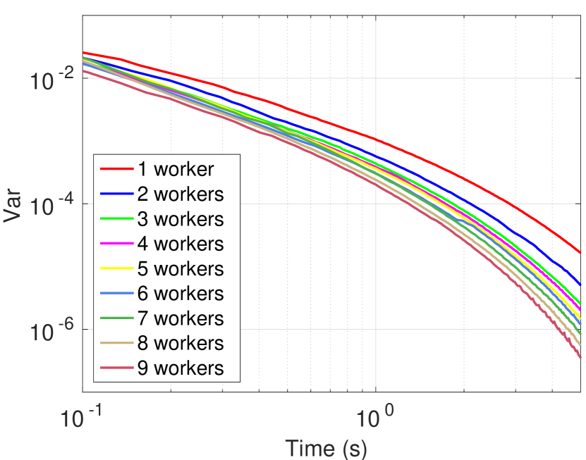
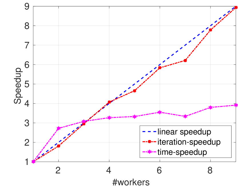
(a) Variance vs. Iteration $\bar{L}$	(b) Variance vs. Time	(c) Speedup

Figure 2: Variance with increasing number of workers.

5.2 Applications to deep learning

We further test S²G-MCMC on Bayesian learning of deep neural networks. The distributed system is developed based on an MPI (message passing interface) extension of the popular Caffe package for deep learning [32]. We implement the SGHMC algorithm, with the point-to-point communications between servers and workers handled by the MPICH library.The algorithm is run on a cluster of five machines. Each machine is equipped with eight 3.60GHz Intel(R) Core(TM) i7-4790 CPU cores.

We evaluate S²G-MCMC on the above BLR model and two deep convolutional neural networks (CNN). In all these models, zero mean and unit variance Gaussian priors are employed for the weights to capture weight uncertainties, an effective way to deal with overfitting [33]. We vary the number of servers $S$ among $\{1,3,5,7\}$, and the number of workers for each server from 1 to 9.

LeNet for MNIST

We modify the standard LeNet to a Bayesian setting for the MNIST dataset.LeNet consists of 2 convolutional layers, 2 max pool layers and 2 ReLU nonlinear layers, followed by 2 fully connected layers [34]. The detailed specification can be found in Caffe. For simplicity, we use the default parameter setting specified in Caffe, with the additional parameter $B$ in SGHMC (Algorithm 1) set to $(1-m)$, where $m$ is the moment variable defined in the SGD algorithm in Caffe.

Cifar10-Quick net for CIFAR10

The Cifar10-Quick net consists of 3 convolutional layers, 3 max pool layers and 3 ReLU nonlinear layers, followed by 2 fully connected layers. The CIFAR-10 dataset consists of 60,000 color images of size 32$\times$32 in 10 classes, with 50,000 for training and 10,000 for testing.Similar to LeNet, default parameter setting specified in Caffe is used.

In these models, the test function is defined as the cross entropy of the softmax outputs $\{\operatorname{\mathbf{o}}_{1},\cdots,\operatorname{\mathbf{o}}_{N}\}$ for test data $\{(\operatorname{\mathbf{d}}_{1},y_{1}),\cdots,(\operatorname{\mathbf{d}}_{N},y_{N})\}$ with $C$ classes, i.e., $\mbox{loss}=-\sum_{i=1}^{N}\operatorname{\mathbf{o}}_{y_{i}}+N\log\sum_{c=1}^{C}e^{\operatorname{\mathbf{o}}_{c}}$. Since the theory indicates a linear speedup on the decrease of variance w.r.t. the number of workers, this means for a single run of the models, the loss would converge faster to its expectation with increasing number of workers. The following experiments verify this intuition.

5.2.1 Single-server experiments

We first test the single-server architecture in Section 4 on the three models. Because the expectations in the bias, MSE or variance are not analytically available in these complex models, we instead plot the loss versus average number of iterations ($\bar{L}$ defined in Section 4) on each worker and the running time in Figure 3. As mentioned above, faster decrease of the loss with more workers is expected.

For the ease of visualization, we only plot the results with $\{1,2,4,6,9\}$ workers; more detailed results are provided in Appendix I. We can see that generally the loss decreases faster with increasing number of workers. In the CIFAR-10 dataset, the final losses of 6 and 9 workers are worst than the one with 4 workers. It shows that the accuracy of the sample average suffers from the increased staleness due to the increased number of workers. Therefore a smaller step size $h$ should be considered to maintain high accuracy when using a large number of workers. Note the 1-worker curves correspond to the standard SG-MCMC, whose loss decreases much slower due to high estimation variance, though in theory it has the same level of bias as the single-server architecture for a given number of iterations (they will converge to the same accuracy).

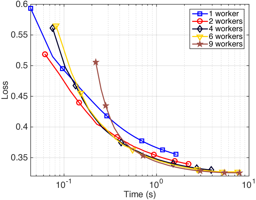
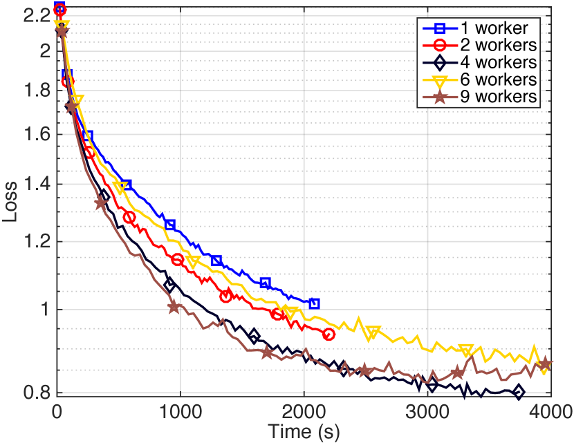
Figure 3: Testing loss vs. #workers. From left to right, each column corresponds to the a9a, MNIST and CIFAR dataset, respectively. The loss is defined in the text.

5.2.2 Multiple-server experiments

Finally, we test the multiple-servers architecture on the same models. We use the same criterion as the single-server setting to measure the convergence behavior. The loss versus average number of iterations on each worker ($\bar{L}$ defined in Section 4) for the three datasets are plotted in Figure 4, where we vary the number of servers among $\{1,3,5,7\}$, and use 2 workers for each server. The plots of loss versus time and using different number of workers for each server are provided in the Appendix. We can see that in the simple BLR model, multiple servers do not seem to show significant speedup, probably due to the simplicity of the posterior, where the sample variance is too small for multiple servers to take effect; while in the more complicated deep neural networks, using more servers results in a faster decrease of the loss, especially in the MNIST dataset.

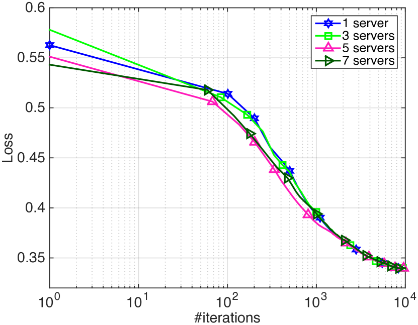
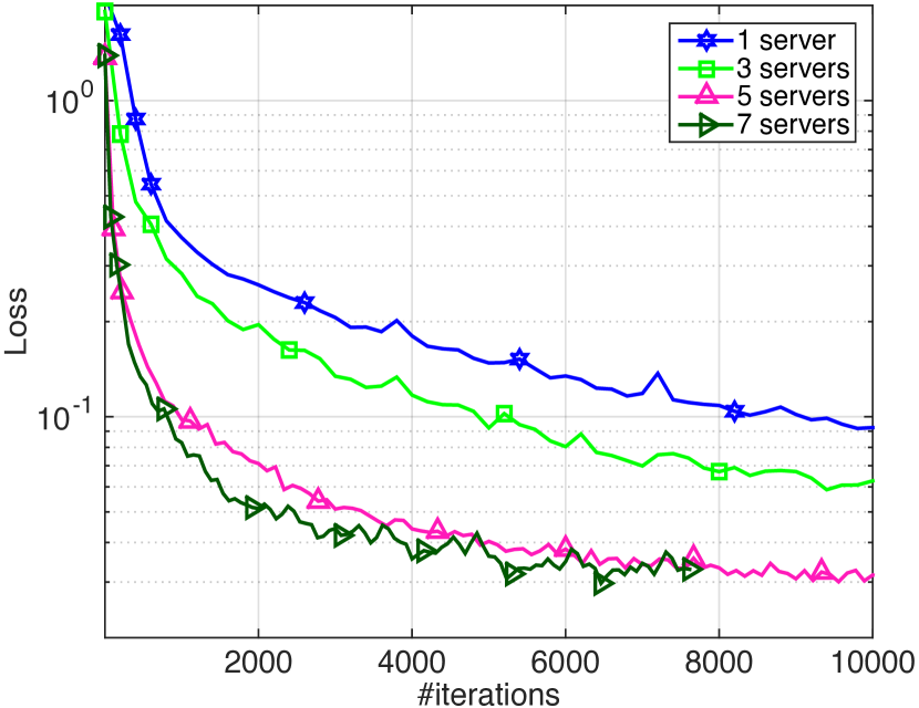
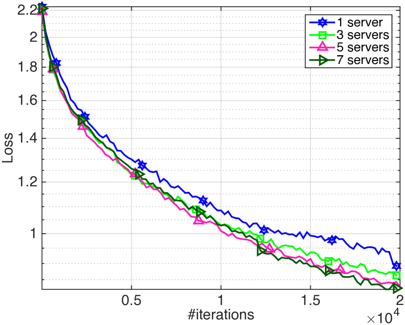
Figure 4: Testing loss vs. #servers. From left to right, each column corresponds to the a9a, MNIST and CIFAR dataset, respectively. The loss is defined in the text.

6 Conclusion

We extend theory from standard SG-MCMC to the stale stochastic gradient setting, and analyze the impacts of the staleness to the convergence behavior of an S²G-MCMC algorithm. Our theory reveals that the estimation variance is independent of the staleness, leading to a linear speedup w.r.t.​ the number of workers, although in practice little speedup in terms of optimal bias and MSE might be achieved due to their dependence on the staleness. We test our theory on a simple asynchronous distributed SG-MCMC system with two simulated examples and several deep neural network models. Experimental results verify the effectiveness and scalability of the proposed S²G-MCMC framework.

Acknowledgements

Supported in part by ARO, DARPA, DOE, NGA, ONR and NSF.

 

Supplementary Material for:
Stochastic Gradient MCMC with Stale Gradients

 

Appendix A A simple Bayesian distributed system based on S²G-MCMC

We provide the detailed architecture of the simple Bayesian distributed system described in Section 4. We put the single-chain and multiple-chain distributed SG-MCMCs into a unified framework. Suppose there are $S$ servers and $W$ workers, the one with $S=1$ corresponds to the single-chain distributed SG-MCMC, whereas the one with $S>1$ corresponds to the multiple-chain distributed SG-MCMC. The servers and workers are responsible for the following tasks:

• Each worker runs independently and communicates with a specific server. They are responsible for computing the stochastic gradients of the parameter given by the server. Once the stochastic gradient is computed, the worker sends it to its assigned server and receive a new parameter sample from the server.

• Each server independently maintains its own state vector and timestamp. At the $l$-th timestamp, it receives a stale stochastic gradient $\nabla_{{\bm{\mathchar 28946\relax}}}\hat{U}_{\tau_{l}}({\bm{\mathchar 28946\relax}})\triangleq\nabla_{{\bm{\mathchar 28946\relax}}}\tilde{U}({\bm{\mathchar 28946\relax}}_{(l-\tau_{l})h})$ from worker $w$, updates the state vector $\operatorname{\mathbf{x}}_{lh}$ to $\operatorname{\mathbf{x}}_{(l+1)h}$ and increments the timestamp, then sends the new parameter sample ${\bm{\mathchar 28946\relax}}_{(l+1)h}$ to worker $w$.

The sending and receiving in the servers and workers are performed asynchronously, enabling minimum communication cost and latency between the servers and workers. At testing, all the samples from the servers are collected and applied to a test function. Apparently, the training time using multiple servers is basically the same as using a single server because the sampling in different servers is independent. Figure 5 depicts the architecture of the proposed Bayesian distributed framework. Algorithm 2 details the algorithm on the servers and workers.

Algorithm 2 Asynchronous Distributed SG-MCMC

   Server

  Output: $\left\{\operatorname{\mathbf{x}}_{h},\ldots,\operatorname{\mathbf{x}}_{Lh}\right\}$

  Initialize $\operatorname{\mathbf{x}}_{0}\in{\mathbf{R}}^{m}$;

  Send ${\bm{\mathchar 28946\relax}}_{0}$ to all assigned workers;

  for $l=0,1,\ldots,L-1$ do

     Receive a stale stochastic gradient $\nabla\tilde{U}_{(l-\tau_{l})h}$ from a worker $w$.

     Update $\operatorname{\mathbf{x}}_{lh}$ to $\operatorname{\mathbf{x}}_{(l+1)h}$ using $\nabla\tilde{U}_{(l-\tau_{l})h}$. (*)

     Send ${\bm{\mathchar 28946\relax}}_{(l+1)h}$ to the worker $w$.

  end for

 

   Worker

  repeat

     Receive ${\bm{\mathchar 28946\relax}}_{lh}$ from server $s$.

     Compute $\nabla\tilde{U}_{lh}$ with a minibatch.

     Send $\nabla\tilde{U}_{lh}$ to server $s$.

  until $stop$

The update rule (*) of the state vector in Algorithm 2 depends on which SG-MCMC algorithm is employed. For instance, Algorithm 1 describes the update rule of the SGHMC with a 1st-order Euler integrator.

Appendix B Assumptions

First, following [25], we will need to assume the corresponding SDE of SG-MCMC to be either elliptic or hypoelliptic. The ellipticity/hypoellipticity describes whether the Brownian motion is able to spread over the whole parameter space. The SDE of the SGLD is elliptic, while for other SG-MCMC algorithms such as the SGHMC, the hypoellipticity assumption is usually reasonable. When the domain $\operatorname{\mathbf{x}}$ is on the torus, the ellipticity and hypoellipticity of an SDE guarantees the existence of a nice solution for the Poisson equation (5). The assumption is summarized in Assumption 2.

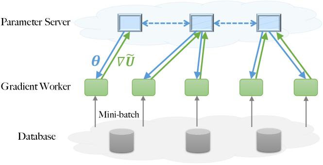
Figure 5: Architecture of the proposed Bayesian distributed framework. In the multi-server case, the dash lines on the servers indicate a simple averaging operation for testing, otherwise the servers are independent. Section 3.3 provides more details.

Assumption 2.

The corresponding SDE of a SG-MCMC algorithm is either elliptic or hypoelliptic.

When $\operatorname{\mathbf{x}}$ is extended to the domain of $\mathbb{R}^{p}$ for some integer $p>0$, we need some assumptions on the solution of the Poisson equation (5). Note (5) can be equivalently written in an integration form [35] using Itô’s formula:

$$\frac{1}{t}\int_{0}^{t}\phi(\operatorname{\mathbf{x}}_{s})\mathrm{d}s-\bar{\phi}$$ (6)

$$= \frac{1}{t}\left(\psi(\operatorname{\mathbf{x}}_{t})-\psi(\operatorname{\mathbf{x}}_{0})\right)-\frac{1}{t}\int_{0}^{t}\nabla\psi(\operatorname{\mathbf{x}}_{s})\cdot g(\operatorname{\mathbf{x}}_{s})\mathrm{d}\mathcal{\operatorname{\mathbf{w}}}_{s}~{}.$$

Intuitively, $\psi$ needs to be bounded if the discrepancy between $\hat{\phi}_{L}$ and $\bar{\phi}$ were to be bounded. This is satisfied if the SDE is defined in a bounded domain [25]. In the unbounded domain as for SG-MCMC algorithms, it turns out the following boundedness assumptions on $\psi$ suffice [17].

Assumption 3.

1) $\psi$ and its up to 3rd-order derivatives, $\mathcal{D}^{k}\psi$, are bounded by a function $\mathcal{V}$, i.e., $\|\mathcal{D}^{k}\psi\|\leq C_{k}\mathcal{V}^{p_{k}}$ for $k=(0,1,2,3)$, $C_{k},p_{k}>0$. 2) the expectation of $\mathcal{V}$ on $\{\operatorname{\mathbf{x}}_{lh}\}$ is bounded: $\sup_{l}\mathbb{E}\mathcal{V}^{p}(\operatorname{\mathbf{x}}_{lh})<\infty$. 3) $\mathcal{V}$ is smooth such that $\sup_{s\in(0,1)}\mathcal{V}^{p}\left(s\operatorname{\mathbf{x}}+\left(1-s\right)\operatorname{\mathbf{y}}\right)\leq C\left(\mathcal{V}^{p}\left(\operatorname{\mathbf{x}}\right)+\mathcal{V}^{p}\left(\operatorname{\mathbf{y}}\right)\right)$, $\forall\operatorname{\mathbf{x}},\operatorname{\mathbf{y}},p\leq\max\{2p_{k}\}$ for some $C>0$.

Furthermore, in our proofs the expectation of a function under a diffusion needs to be expanded in a Taylor expansion style, e.g., $\mathbb{E}\phi(\operatorname{\mathbf{x}}_{t})=\sum_{i=0}^{\ell}\frac{t^{i}}{i!}\mathcal{L}^{i}\phi(\operatorname{\mathbf{x}}_{0})+t^{\ell+1}r_{\ell,F,\phi}(\operatorname{\mathbf{x}}_{0})$ by using Kolmogorov’s backward equation. To ensure the remainder term $r_{\ell,F,\phi}(\operatorname{\mathbf{x}}_{0})$ to be bounded, it suffices to make the following assumption on the smoothness and boundedness of $F(\operatorname{\mathbf{x}})$ [35, 17].

Assumption 4.

$F(\operatorname{\mathbf{x}})$ is infinitely differentiable with bounded derivatives of any order; and $|F(\operatorname{\mathbf{x}})|\leq A(1+|\operatorname{\mathbf{x}}|^{s})$ for some integer $s>0$ and $A>0$.

Appendix C Notation

For simplicity, we will simplify some notation used in the proof as follows:

$$\nabla_{{\bm{\mathchar 28946\relax}}}\tilde{U}_{l}({\bm{\mathchar 28946\relax}}_{lh})\triangleq\nabla_{{\bm{\mathchar 28946\relax}}}\tilde{U}_{lh}\triangleq\tilde{G}_{lh}$$

$$\nabla_{{\bm{\mathchar 28946\relax}}}U_{l}({\bm{\mathchar 28946\relax}}_{lh})\triangleq\nabla_{{\bm{\mathchar 28946\relax}}}U_{lh}\triangleq G_{lh}$$

$$\psi(\operatorname{\mathbf{X}}_{lh})\triangleq\psi_{lh}$$

Appendix D Proof of Theorem 2

In S²G-MCMC, for the $l$-th iteration, suppose a stochastic gradient with a staleness $\tau_{l}$ is used, e.g., $\tilde{G}_{(l-\tau_{l})h}$. First, we will bound the difference between $\tilde{G}_{(l-\tau_{l})h}$ and the stochastic gradient at the $l$-th iteration $\tilde{G}_{lh}$, by using the Lipschitz property of $\tilde{G}_{lh}$, with the following lemma.

Lemma 8.

Let $f_{lh}\triangleq\left\|\operatorname{\mathbf{x}}_{lh}-\operatorname{\mathbf{x}}_{(l-1)h}\right\|$, the expected difference between $\tilde{G}_{(l-\tau_{l})h}$ and $\tilde{G}_{lh}$ is bounded by:

$$\left\|\mathbb{E}\left(\tilde{G}_{(l-\tau_{l})h}-\tilde{G}_{lh}\right)\right\|=\max_{i=l-\tau_{l}}^{l-1}\left|\mathcal{L}_{i}f_{ih}\right|C\tau h+O(h^{2}),$$ (7)

where the expectation is taken over the randomness of the SG-MCMC algorithm, e.g., the randomness from stochastic gradients and the injected Gaussian noise.

Proof.

Note the randomness of $\tilde{G}_{lh}$ comes from two sources, the injected Gaussian noise and the stochastic gradient noise. We denote the expectations with respect to these two randomness as $\mathbb{E}_{\zeta}$ and $\mathbb{E}_{g}$, respectively. The whole expectation thus can be decomposed as $\mathbb{E}=\mathbb{E}_{\zeta}\mathbb{E}_{g}$.

Applying the Lipschitz property of $\tilde{G}_{lh}$, we have

$$\left\|\mathbb{E}\left(\tilde{G}_{(l-\tau_{l})h}-\tilde{G}_{lh}\right)\right\|=\left\|\mathbb{E}_{\zeta}\left(G_{(l-\tau_{l})h}-G_{lh}\right)\right\|$$

$$\leq\mathbb{E}_{\zeta}\left\|\left(G_{(l-\tau_{l})h}-G_{lh}\right)\right\|$$

$$\leq C\mathbb{E}_{\zeta}\left\|\left({\bm{\mathchar 28946\relax}}_{(l-\tau_{l})h}-\mathchar 28946\relax_{lh}\right)\right\|$$

$$\leq C\mathbb{E}_{\zeta}\left\|\sum_{i=l-\tau_{l}}^{l-1}\left({\bm{\mathchar 28946\relax}}_{(ih)}-{\bm{\mathchar 28946\relax}}_{(i+1)h}\right)\right\|$$

$$\leq C\sum_{i=l-\tau_{l}}^{l-1}\mathbb{E}_{\zeta}\left\|\left({\bm{\mathchar 28946\relax}}_{(ih)}-{\bm{\mathchar 28946\relax}}_{(i+1)h}\right)\right\|$$

$$\leq C\sum_{i=l-\tau_{l}}^{l-1}\mathbb{E}_{\zeta}\left\|\operatorname{\mathbf{x}}_{(i+1)h}-\operatorname{\mathbf{x}}_{ih}\right\|$$

From the definition of $K$th-order integrator, i.e., $\mathbb{E}_{\zeta}f(\operatorname{\mathbf{x}}_{lh})=e^{\tilde{\mathcal{L}}_{l}h}f(\operatorname{\mathbf{x}}_{(l-1)h})+O(h^{K+1})$, if we let

$$f(\operatorname{\mathbf{x}}_{lh})=\left\|\operatorname{\mathbf{x}}_{lh}-\operatorname{\mathbf{x}}_{(l-1)h}\right\|\triangleq f_{lh}~{},$$

where $\operatorname{\mathbf{x}}_{(l-1)h}$ is the starting point in the $l$-th iteration, and note that

$$f(\operatorname{\mathbf{x}}_{(l-1)h})=0~{}.$$

We have

$$C\sum_{i=l-\tau_{l}}^{l-1}\mathbb{E}_{\zeta}\left\|\operatorname{\mathbf{x}}_{(i+1)h}-\operatorname{\mathbf{x}}_{ih}\right\|\triangleq C\sum_{i=l-\tau_{l}}^{l-1}\mathbb{E}_{\zeta}f(\operatorname{\mathbf{x}}_{lh})$$ (8)

$$\leq C\sum_{i=l-\tau_{l}}^{l-1}\left(e^{\mathcal{L}_{i}h}f(\operatorname{\mathbf{x}}_{(i-1)h})+O(h^{K+1})\right)$$ (9)

$$\leq C\sum_{i=l-\tau_{l}}^{l-1}\left|\mathcal{L}_{i}f_{ih}\right|h+O(h^{2})$$ (10)

$$\leq \max_{i=l-\tau_{l}}^{l-1}\left|\mathcal{L}_{i}f_{ih}\right|C\tau h+O(h^{2})~{},$$

where (10) is obtained by expanding the exponential operator and the assumption that the high order terms are bounded. ∎

Now we proceed to prove Theorem 2. The basic technique follows [17], thus we skip some derivations for some steps.

Proof of Theorem 2.

Before the proof, let us first define some notation. First, define the operator $\Delta V_{l}$ for each $l$ as a differential operator as for any function $\psi$:

$$\Delta V_{l}\psi\triangleq\left(\tilde{G}_{l-\tau_{l}}-G_{l}\right)\cdot\nabla_{\operatorname{\mathbf{p}}}\psi~{}.$$

Second, define the local generator, $\tilde{\mathcal{L}}_{l}$, for an Itô diffusion, where the true gradient in (1) is replaced with the stochastic gradient from the $l$-th iteration, i.e., $\tilde{\mathcal{L}}_{l}f(\operatorname{\mathbf{X}}_{t})\triangleq$

$$\left(\tilde{F}_{l}(\operatorname{\mathbf{x}}_{t})\cdot\nabla+\frac{1}{2}\left(\sigma(\operatorname{\mathbf{x}}_{t})\sigma(\operatorname{\mathbf{x}}_{t})^{T}\right)\!:\!\nabla\nabla^{T}\right)f(\operatorname{\mathbf{x}}_{t})~{},$$

for a compactly supported twice differentiable function $f$, where $\tilde{F}_{l}$ is the same as $F$ but with the full gradient $G_{lh}$ replaced with the stochastic gradient $\tilde{G}_{lh}$. Based on these definitions, we have

$$\tilde{\mathcal{L}}_{l}=\mathcal{L}+\Delta V_{l}~{}.$$

Following [17], for an SG-MCMC with a $K$th-order integrator, and a test function $\phi$, we have:

$$\mathbb{E} [\psi(\operatorname{\mathbf{x}}_{lh})]=\left(\mathbb{I}+h\tilde{\operatorname{\mathcal{L}}}_{l}\right)\psi(\operatorname{\mathbf{x}}_{(l-1)h})$$ (11)

$$+\sum_{k=2}^{K}\frac{h^{k}}{k!}\tilde{\operatorname{\mathcal{L}}}_{l}^{k}\psi(\operatorname{\mathbf{x}}_{(l-1)h})+O\left(\frac{h^{K+1}}{(K+1)!}\tilde{\operatorname{\mathcal{L}}}_{l}^{K+1}\psi_{(l-1)h}\right)~{},$$

where $\mathbb{I}$ is the identity map. Sum over $l=1,\cdots,L$ in (11), take expectation on both sides, and use the relation $\tilde{\operatorname{\mathcal{L}}}_{l}=\operatorname{\mathcal{L}}+\Delta V_{l}$ to expand the first order term. We obtain

$$\sum_{l=1}^{L}\mathbb{E} [\psi(\operatorname{\mathbf{x}}_{lh})]=\psi(\operatorname{\mathbf{x}}_{0})+\sum_{l=1}^{L-1}\mathbb{E}[\psi(\operatorname{\mathbf{x}}_{lh})]$$

$$+h\sum_{l=1}^{L}\mathbb{E}[\mathcal{L}\psi(\operatorname{\mathbf{x}}_{(l-1)h})]+h\sum_{l=1}^{L}\mathbb{E}[\Delta V_{l}\psi(\operatorname{\mathbf{x}}_{(l-1)h})]$$

$$+\sum_{k=2}^{K}\frac{h^{k}}{k!}\sum_{l=1}^{L}\operatorname{\mathbb{E}}[\tilde{\operatorname{\mathcal{L}}}_{l}^{k}\psi(\operatorname{\mathbf{x}}_{(l-1)h})]$$

$$+O\left(\frac{h^{K+1}}{(K+1)!}\sum_{l}\mathbb{E}\tilde{\operatorname{\mathcal{L}}}_{l}^{K+1}\psi_{(l-1)h}\right).$$

Divide both sides by $Lh$, use the Poisson equation (5), and reorganize terms. We have:

$$\mathbb{E}[\frac{1}{L}\sum_{l}\phi(\operatorname{\mathbf{x}}_{lh})-\bar{\phi}]=\frac{1}{L}\sum_{l=1}^{L}\mathbb{E}[\mathcal{L}\psi(\operatorname{\mathbf{x}}_{(l-1)h})]$$ (12)

$$= \frac{1}{Lh}\left(\mathbb{E}[\psi(\operatorname{\mathbf{x}}_{lh})]-\psi(\operatorname{\mathbf{x}}_{0})\right)-\frac{1}{L}\sum_{l}\mathbb{E}[\Delta V_{l}\psi(\operatorname{\mathbf{x}}_{(l-1)h})]$$

$$-\sum_{k=2}^{K}\frac{h^{k-1}}{k!L}\sum_{l=1}^{L}\operatorname{\mathbb{E}}[\tilde{\operatorname{\mathcal{L}}}_{l}^{k}\psi(\operatorname{\mathbf{x}}_{(l-1)h})]+O\left(\frac{h^{K}}{(K+1)!L}\sum_{l}\mathbb{E}\tilde{\operatorname{\mathcal{L}}}_{l}^{K+1}\psi_{(l-1)h}\right)$$

According to [17], the term $\sum_{l}\mathbb{E}[\tilde{\operatorname{\mathcal{L}}}_{l}^{k}\psi(\operatorname{\mathbf{x}}_{(l-1)h})]$ is bounded by $\sum_{l}\mathbb{E}[\tilde{\operatorname{\mathcal{L}}}_{l}^{k}\psi(\operatorname{\mathbf{X}}_{(l-1)h})]$

$$=O\left(\frac{1}{h}+h^{K-k+1}\sum_{l}\mathbb{E}\tilde{\operatorname{\mathcal{L}}}_{l}^{K+1}\psi_{(l-1)h}\right)~{},$$ (13)

Substituting (13) into (12), after simplification, we have: $\mathbb{E}\left(\frac{1}{L}\sum_{l}\phi(\operatorname{\mathbf{x}}_{lh})-\bar{\phi}\right)$

$$= \frac{1}{Lh}\underbrace{\left(\mathbb{E}[\psi(\operatorname{\mathbf{x}}_{lh})]-\psi(\operatorname{\mathbf{x}}_{0})\right)}_{C_{1}}-\underbrace{\frac{1}{L}\sum_{l}\mathbb{E}[\Delta V_{l}\psi(\operatorname{\mathbf{x}}_{(l-1)h})]}_{C_{2}}$$

$$-\sum_{k=2}^{K}O\left(\frac{h^{k-1}}{Lh}+\frac{h^{K}}{L}\sum_{l}\frac{1}{k!}\mathbb{E}\tilde{\operatorname{\mathcal{L}}}_{l}^{K}\psi_{(l-1)h}\right)+\frac{h^{K}}{(K+1)!L}\sum_{l}\mathbb{E}\tilde{\operatorname{\mathcal{L}}}_{l}^{K+1}\psi_{(l-1)h}~{},$$

According to the assumption, the term $C_{1}$ is bounded. For term $C_{2}$, according to the Cauchy–Schwarz inequality, we have

$$\left|C_{2}\right|=\frac{1}{L}\left|\sum_{l}\mathbb{E}\left(\tilde{G}_{(l-\tau_{l})h}-G_{lh}\right)\cdot\mathbb{E}\nabla\psi_{(l-1)h}\right|$$

$$\leq \frac{1}{L}\sum_{l}\left|\mathbb{E}\left(\tilde{G}_{(l-\tau_{l})h}-G_{lh}\right)\cdot\mathbb{E}\nabla\psi_{(l-1)h}\right|$$

$$\leq \frac{1}{L}\sum_{l}\left\|\mathbb{E}\left(\tilde{G}_{(l-\tau_{l})h}-G_{lh}\right)\right\|\left\|\mathbb{E}\nabla\psi_{(l-1)h}\right\|$$

$$\leq \frac{1}{L}\sum_{l}\left(\left\|\mathbb{E}\left(\tilde{G}_{(l-\tau_{l})h}-\tilde{G}_{lh}\right)\right\|+\left\|\mathbb{E}\left(\tilde{G}_{lh}-G_{lh}\right)\right\|\right)\left\|\mathbb{E}\nabla\psi_{(l-1)h}\right\|$$

$$= \frac{1}{L}\sum_{l}\left\|\mathbb{E}\left(\tilde{G}_{(l-\tau_{l})h}-\tilde{G}_{lh}\right)\right\|\left\|\mathbb{E}\nabla\psi_{(l-1)h}\right\|$$

Applying (7) from Lemma 8, we have

$$\left|C_{2}\right| \leq\frac{1}{L}\sum_{l}\left(\max_{i=l-\tau_{l}}^{l}\left\|\mathcal{L}_{i}\right\|\left\|\mathbb{E}\nabla\psi_{lh}\right\|C\tau_{l}h\right)$$

$$\leq\max_{l}\left\|\mathcal{L}_{l}\right\|\max_{l}\left\|\mathbb{E}\nabla\psi_{lh}\right\|C\tau h~{}.$$

As a result, collecting low order terms, the bias can be expressed as:

$$\left|\mathbb{E}\hat{\phi}-\bar{\phi}\right|=\left|\mathbb{E}\left(\frac{1}{L}\sum_{l}\phi(\operatorname{\mathbf{x}}_{lh})-\bar{\phi}\right)\right|$$

$$= \left|\frac{C_{1}}{Lh}-C_{2}+h^{K}\sum_{k=1}^{K}\frac{1}{(k+1)!L}\sum_{l}\mathbb{E}\tilde{\operatorname{\mathcal{L}}}_{l}^{k+1}\psi_{(l-1)h}\right|~{}.$$

As a result, there exists some constant $D_{1}$ independent of $(L,h,\tau)$, such that

$$\left|\mathbb{E}\hat{\phi}-\bar{\phi}\right|\leq D_{1}\left|\frac{1}{Lh}\right|+\left|C_{2}\right|+\left|M_{1}\tau h+\left|M_{2}h^{K}\right|\right|$$ (15)

$$= D_{1}\left(\frac{1}{Lh}+M_{1}\tau h+M_{2}h^{K}\right)~{},$$

where $M_{1}\triangleq\max_{l}\left\|\mathcal{L}_{l}\right\|\max_{l}\left\|\mathbb{E}\nabla\psi_{lh}\right\|C$, $M_{2}\triangleq\sum_{k=1}^{K}\frac{1}{(k+1)!L}\sum_{l}\mathbb{E}\tilde{\operatorname{\mathcal{L}}}_{l}^{k+1}\psi_{(l-1)h}$. (15) follows by substituting the inequality for $C_{2}$ above. This completes the proof. ∎

Appendix E Proof of Theorem 3

Proof.

Similar to the proof of Theorem 2, we first expand $\mathbb{E}\psi_{lh}$ using the property of $K$th-order integrator as

$$\sum_{l=1}^{L} \mathbb{E}\left(\psi(\operatorname{\mathbf{x}}_{lh})\right)=\sum_{l=1}^{L}\psi(\operatorname{\mathbf{x}}_{(l-1)h})+h\sum_{l=1}^{L}\mathcal{L}\psi(\operatorname{\mathbf{x}}_{(l-1)h})$$

$$+h\sum_{l=1}^{L}\Delta V_{l}\psi(\operatorname{\mathbf{x}}_{(l-1)h})+\sum_{k=2}^{K}\frac{h^{k}}{k!}\sum_{l=1}^{L}\tilde{\mathcal{L}}_{l}^{k}\psi(\operatorname{\mathbf{x}}_{(l-1)h})$$

$$+O\left(\frac{h^{K+1}}{(K+1)!}\sum_{l}\tilde{\operatorname{\mathcal{L}}}_{l}^{K+1}\psi_{(l-1)h}\right)~{}.$$

Substituting the Poisson equation (5) into the above equation, dividing both sides by $Lh$ and rearranging related terms arrives

$$\hat{\phi}- \bar{\phi}=\frac{1}{Lh}\left(\mathbb{E}\psi(\operatorname{\mathbf{x}}_{Lh})-\psi(\operatorname{\mathbf{x}}_{0})\right)$$ (16)

$$- \frac{1}{Lh}\sum_{l=1}^{L}\left(\mathbb{E}\psi_{(l-1)h}-\psi_{(l-1)h}\right)-\frac{1}{L}\sum_{l=1}^{L}\Delta V_{l}\psi_{(l-1)h}$$

$$- \sum_{k=2}^{K}\frac{h^{k-1}}{2L}\sum_{l=1}^{L}\tilde{\mathcal{L}}_{l}^{k}\psi(\operatorname{\mathbf{x}}_{(l-1)h})+O\left(\frac{h^{K}}{L(K+1)!}\sum_{l}\tilde{\operatorname{\mathcal{L}}}_{l}^{K+1}\psi_{(l-1)h}\right)$$

Taking square on both sides, we have there exists some positive constant $D$, such that

$$\left(\hat{\phi}-\bar{\phi}\right)^{2}\leq D\left(\underbrace{\frac{\left(\mathbb{E}\psi_{Lh}-\psi_{0}\right)^{2}}{L^{2}h^{2}}}_{A_{1}}+\underbrace{\frac{1}{L^{2}h^{2}}\sum_{l=1}^{L}\left(\mathbb{E}\psi_{(l-1)h}-\psi_{(l-1)h}\right)^{2}}_{A_{2}}\right.$$

$$+ \left.\underbrace{\left(\frac{1}{L}\sum_{l=1}^{L}\Delta V_{l}\psi_{(l-1)h}\right)^{2}}_{A_{3}}+\underbrace{\sum_{k=2}^{K}\frac{h^{2(k-1)}}{k!L^{2}}\left(\sum_{l=1}^{L}\tilde{\mathcal{L}}_{l}^{k}\psi_{(l-1)h}\right)^{2}}_{A_{4}}+\underbrace{\left(\frac{\sum_{l}\tilde{\operatorname{\mathcal{L}}}_{l}^{K+1}\psi_{(l-1)h}}{L(K+1)!}\right)^{2}h^{2K}}_{A_{5}}\right)$$ (17)

After taking expectation, we have

$$\mathbb{E}\left(\hat{\phi}-\bar{\phi}\right)^{2}\leq C\left(\mathbb{E}A_{1}+\mathbb{E}A_{2}+\mathbb{E}A_{3}+\mathbb{E}A_{4}+\mathbb{E}A_{5}\right)$$

$A_{1}$ is easily bounded by the assumption that $\|\psi\|\leq V^{p_{0}}<\infty$. From the proof of Theorem 3 in [17], $A_{2}$ and $A_{4}$ are also bounded, which are summarized in Lemma 9.

Lemma 9.

The terms $\mathbb{E}A_{2}$ and $\mathbb{E}A_{4}$ are bounded by:

$$\mathbb{E}A_{2} =O\left(\frac{1}{Lh}\right)$$

$$\mathbb{E}A_{4} =O\left(\frac{1}{Lh}+h^{2K}\sum_{k=2}^{K}\frac{1}{Lk!}\sum_{l}\tilde{\operatorname{\mathcal{L}}}_{l}^{k+1}\psi_{(l-1)h}\right)~{}.$$

We are left to show a bound for $\mathbb{E}A_{3}$. First we have

$$\mathbb{E}A_{3}=\mathbb{E}\left(\frac{1}{L}\sum_{l=1}^{L}\Delta V_{l}\psi_{(l-1)h}\right)^{2}$$

$$= \mathbb{E}\left(\frac{1}{L}\sum_{l=1}^{L}\left(\tilde{G}_{(l-\tau_{l})h}-G_{lh}\right)\cdot\nabla_{\operatorname{\mathbf{p}}}\psi_{(l-1)h}\right)^{2}$$

$$= \frac{1}{L^{2}}\sum_{i=1}^{L}\sum_{j=1}^{L}\mathbb{E}\left[\left(\tilde{G}_{(i-\tau_{i})h}-G_{ih}\right)\cdot\nabla_{\operatorname{\mathbf{p}}}\psi_{(i-1)h}\left(\tilde{G}_{(j-\tau_{j})h}-G_{jh}\right)\cdot\nabla_{\operatorname{\mathbf{p}}}\psi_{(j-1)h}\right]$$

Using the Cauchy–Schwartz inequality, we have

$$\leq \frac{1}{L^{2}}\sum_{i=1}^{L}\sum_{j=1}^{L}\left\|\mathbb{E}\left(\tilde{G}_{(i-\tau_{i})h}-G_{ih}\right)\right\|\left\|\mathbb{E}\left(\tilde{G}_{(j-\tau_{j})h}-G_{jh}\right)\right\|\left\|\mathbb{E}\nabla\psi_{(i-1)h}\right\|\left\|\mathbb{E}\nabla\psi_{(j-1)h}\right\|$$

$$\leq \frac{1}{L^{2}}\sum_{i=1}^{L}\sum_{j=1}^{L}\left(\left\|\mathbb{E}\left(\tilde{G}_{(i-\tau_{i})h}-\tilde{G}_{ih}\right)\right\|+\left\|\mathbb{E}\left(\tilde{G}_{ih}-G_{ih}\right)\right\|\right)$$

$$\left(\left\|\mathbb{E}\left(\tilde{G}_{(j-\tau_{j})h}-\tilde{G}_{jh}\right)\right\|+\left\|\mathbb{E}\left(\tilde{G}_{jh}-G_{jh}\right)\right\|\right)\left\|\mathbb{E}\nabla\psi_{(i-1)h}\right\|\left\|\mathbb{E}\nabla\psi_{(j-1)h}\right\|$$

$$= \frac{1}{L^{2}}\sum_{i=1}^{L}\sum_{j=1}^{L}\left\|\mathbb{E}\left(\tilde{G}_{(i-\tau_{i})h}-\tilde{G}_{ih}\right)\right\|\left\|\mathbb{E}\left(\tilde{G}_{(j-\tau_{j})h}-\tilde{G}_{jh}\right)\right\|\left\|\mathbb{E}\nabla\psi_{(i-1)h}\right\|\left\|\mathbb{E}\nabla\psi_{(j-1)h}\right\|$$

Applying (7) from Lemma 8, we have

$$\mathbb{E}A_{3}\leq\max_{l}\left\|\mathbb{E}\nabla\psi_{lh}\right\|^{2}\max_{l}\left(\mathcal{L}_{l}f_{lh}\right)^{2}C^{2}\tau^{2}h^{2}~{}.$$

Collecting low order terms from the above bounds, we have there exists some constant $D_{2}$ independent of $(L,h,\tau)$, such that

$$\mathbb{E}\left(\hat{\phi}-\bar{\phi}\right)^{2}$$

$$\leq \frac{C_{1}}{Lh}+C_{2}h^{2K}+\max_{l}\left\|\mathbb{E}\nabla\psi_{lh}\right\|^{2}\max_{l}\left\|\mathcal{L}_{l}\right\|^{2}C^{2}\tau^{2}h^{2}$$

$$\leq D_{2}\left(\frac{1}{Lh}+\tilde{M}_{1}\tau^{2}h^{2}+\tilde{M}_{2}h^{2K}\right)~{},$$

where $\tilde{M}_{1}\triangleq\max_{l}\left\|\mathbb{E}\nabla\psi_{lh}\right\|^{2}\max_{l}\left(\mathcal{L}_{l}f_{lh}\right)^{2}C^{2}$, $\tilde{M}_{2}\triangleq\mathbb{E}\left(\frac{1}{L(K+1)!}\sum_{l}\tilde{\operatorname{\mathcal{L}}}_{l}^{K+1}\psi_{(l-1)h}\right)^{2}$. This completes the proof. ∎

Appendix F Proof of Theorem 4

In the proof, we will use the following simple result stated Lemma 10.

Lemma 10.

Let $(\mathcal{M}_{1},\cdots,\mathcal{M}_{N})$ be a set of independent martingale, i.e, $\mathbb{E}\left[\mathcal{M}_{n}|\mathcal{F}\right]=0$, where $\mathcal{F}$ is the filtration generated by $\mathcal{M}_{n}$. Then we have

$$\mathbb{E}\left[\left(\sum_{n=1}^{N}\mathcal{M}_{n}\right)^{2}|\mathcal{F}\right]=\sum_{n=1}^{N}\mathbb{E}\left[\mathcal{M}_{n}^{2}|\mathcal{F}\right]~{}.$$ (18)

Proof.

$$\mathbb{E}\left[\left(\sum_{n=1}^{N}\mathcal{M}_{n}\right)^{2}|\mathcal{F}\right]=\mathbb{E}\left[\sum_{i=1}^{N}\sum_{j=1}^{N}\mathcal{M}_{i}\mathcal{M}_{j}|\mathcal{F}\right]$$

$$= \mathbb{E}\left[\sum_{i=1}^{N}\mathcal{M}_{i}^{2}|\mathcal{F}\right]+\sum_{i\neq j}\mathbb{E}\left[\mathcal{M}_{i}|\mathcal{F}\right]\mathbb{E}\left[\mathcal{M}_{j}|\mathcal{F}\right]$$

$$= \sum_{i=1}^{N}\mathbb{E}\left[\mathcal{M}_{i}^{2}|\mathcal{F}\right]~{}.$$

∎

In the following we will omitted the filtration $\mathcal{F}$ in the expectation for simplicity. We we now ready to prove Theorem 4.

Proof.

By definition, we have

$$\mbox{Var}\left(\hat{\phi}_{L}\right)=\mathbb{E}\left(\hat{\phi}_{L}-\bar{\phi}-\left(\mathbb{E}\hat{\phi}_{L}-\bar{\phi}\right)\right)^{2}$$

Substitute (12) and (16) into the above equation, we have

$$\hat{\phi}_{L} -\mathbb{E}\bar{\phi}=-\frac{1}{Lh}\sum_{l}\left(\mathbb{E}\psi_{(l-1)h}-\psi_{(l-1)h}\right)$$

$$-\frac{1}{L}\sum_{l}\left(A_{1}-\mathbb{E}A_{1}\right)-\sum_{k}\frac{h^{k-1}}{k!L}\sum_{l}\left(A_{2}-\mathbb{E}A_{2}\right)-\frac{h^{K}}{(K+1)!L}\sum_{l}\left(A_{3}-\mathbb{E}A_{3}\right)~{},$$

where

$$A_{1} \triangleq\Delta V_{l}\psi_{(l-1)h}$$

$$A_{2} \triangleq\tilde{\mathcal{L}}_{l}^{k}\psi_{(l-1)h}$$

$$A_{3} \triangleq\tilde{\mathcal{L}}_{l}^{K+1}\psi_{(l-1)h}~{}.$$

Take square on both sides, following by expectation, and note that all $(A_{i}-\mathbb{E}A_{i})$ are martingale for $i=1,2,3$, which allows us to use (18) from Lemma 10. We have there exists a constant $D$ independent of $(L,h,\tau)$, such that

$$\mbox{Var}\left(\hat{\phi}_{L}\right)\leq D\left(\frac{1}{L^{2}h^{2}}\mathbb{E}\left(\sum_{l}\left(\mathbb{E}\psi_{(l-1)h}-\psi_{(l-1)h}\right)\right)^{2}\right.$$

$$+\frac{1}{L^{2}}\sum_{l}\mathbb{E}\left(A_{1}-\mathbb{E}A_{1}\right)^{2}+\sum_{k}\frac{h^{2(k-1)}}{(k!L)2}\sum_{l}\mathbb{E}\left(A_{2}-\mathbb{E}A_{2}\right)^{2}$$

$$\left.+\frac{h^{2K}}{((K+1)!L)^{2}}\sum_{l}\mathbb{E}\left(A_{3}-\mathbb{E}A_{3}\right)^{2}\right)$$

$$\leq D\left(\underbrace{\frac{1}{L^{2}h^{2}}\mathbb{E}\left(\sum_{l}\left(\mathbb{E}\psi_{(l-1)h}-\psi_{(l-1)h}\right)\right)^{2}}_{B_{1}}\right.$$

$$~{}~{}~{}~{}+\left.\frac{1}{L^{2}}\sum_{l}\mathbb{E}\left(A_{1}-\mathbb{E}A_{1}\right)^{2}+\sum_{k=2}^{K}\frac{h^{2(k-1)}}{(k!L)2}\sum_{l}\mathbb{E}A_{2}^{2}+\frac{h^{2K}}{((K+1)!L)^{2}}\sum_{l}\mathbb{E}A_{3}^{2}\right)~{}.$$

According to Lemma 9, $B_{1}$ is bounded by

$$B_{1}=O\left(\frac{1}{Lh}\right)~{}.$$

Furthermore, according to the assumptions, both $\mathbb{E}A_{2}^{2}$ and $\mathbb{E}A_{3}^{2}$ are bounded. The delayed parameter $\tau$ exists in $\mathbb{E}\left(A_{1}-\mathbb{E}A_{1}\right)^{2}$, we have

$$\mathbb{E}\left(A_{1}-\mathbb{E}A_{1}\right)^{2}$$

$$= \mathbb{E}\left(\Delta V_{l}\psi_{(l-1)h}-\mathbb{E}\Delta V_{l}\psi_{(l-1)h}\right)^{2}$$

$$= \mathbb{E}\left(\left(\tilde{G}_{(l-\tau_{l})h}-G_{lh}\right)\cdot\nabla_{\operatorname{\mathbf{p}}}\psi_{(l-1)h}-\mathbb{E}\left(\tilde{G}_{(l-\tau_{l})h}-G_{lh}\right)\cdot\nabla_{\operatorname{\mathbf{p}}}\psi_{(l-1)h}\right)^{2}$$

Expanding the terms, we have there exists a constant $D_{1}$ such that

$$\mathbb{E}\left(A_{1}-\mathbb{E}A_{1}\right)^{2}$$

$$\leq D_{1}\mathbb{E}\left(\tilde{G}_{(l-\tau_{l})h}\cdot\nabla_{\operatorname{\mathbf{p}}}\psi_{(l-1)h}-\mathbb{E}\tilde{G}_{(l-\tau_{l})h}\cdot\nabla_{\operatorname{\mathbf{p}}}\psi_{(l-1)h}\right)^{2}$$

$$~{}~{}+D_{1}\mathbb{E}\left(G_{lh}\cdot\nabla_{\operatorname{\mathbf{p}}}\psi_{(l-1)h}-\mathbb{E}G_{lh}\cdot\nabla_{\operatorname{\mathbf{p}}}\psi_{(l-1)h}\right)^{2}$$

$$= D_{1}\mathbb{E}\left(\tilde{G}_{(l-\tau_{l})h}\cdot\nabla_{\operatorname{\mathbf{p}}}\psi_{(l-1)h}\right)^{2}+D_{1}\mathbb{E}\left(G_{lh}\cdot\left(\nabla_{\operatorname{\mathbf{p}}}\psi_{(l-1)h}-\nabla_{\operatorname{\mathbf{p}}}\psi_{(l-1)h}\right)\right)^{2}$$

$$\leq D_{1}\left(\mathbb{E}\left\|\tilde{G}_{(l-\tau_{l})h}\right\|^{2}\mathbb{E}\left\|\nabla_{\operatorname{\mathbf{p}}}\psi_{(l-1)h}\right\|^{2}+\mathbb{E}\left\|G_{lh}\right\|^{2}\mathbb{E}\left\|\nabla_{\operatorname{\mathbf{p}}}\psi_{(l-1)h}-\nabla_{\operatorname{\mathbf{p}}}\psi_{(l-1)h}\right\|^{2}\right)$$

$$\leq D_{1}\sup_{l}\left\{\mathbb{E}\left\|\tilde{G}_{lh}\right\|^{2}\mathbb{E}\left\|\nabla_{\operatorname{\mathbf{p}}}\psi_{lh}\right\|^{2}+\mathbb{E}\left\|G_{lh}\right\|^{2}\mathbb{E}\left\|\nabla_{\operatorname{\mathbf{p}}}\psi_{lh}\right\|^{2}\right\}~{}.$$

According to the assumptions, the above bound is bounded, and does not depend on $\tau$. As a result,

$$\frac{1}{L^{2}}\sum_{l}\mathbb{E}\left(A_{1}-\mathbb{E}A_{1}\right)^{2}\leq\frac{D_{1}}{L}~{}.$$

In addition, the bounds for both $\mathbb{E}A_{2}^{2}$ and $\mathbb{E}A_{3}^{2}$ are given in Lemma 9, which are higher-order terms with respect to $h$, i.e., $O\left(h^{2K}\right)$.

Collecting low order terms, we have there exists a constant $D$ independent of $(L,h,\tau)$, such that the variance is bounded by:

$$\mbox{Var}\left(\hat{\phi}_{L}\right)\leq D\left(\frac{1}{Lh}+h^{2K}\right)=D\left(\frac{1}{W\bar{L}h}+h^{2K}\right)~{}.$$

∎

Appendix G Proof of Theorem 6

We separate the proof for the bias and MSE, respectively.

Proof for the bias.

According to the definition of $\hat{\phi}_{L}^{S}$, we have

$$\left|\mathbb{E}\hat{\phi}_{L}^{S}-\bar{\phi}\right|=\left|\mathbb{E}\sum_{s=1}^{S}\frac{T_{s}}{T}\hat{\phi}_{L_{s}}-\bar{\phi}\right|$$

$$= \left|\sum_{s=1}^{S}\frac{T_{s}}{T}\mathbb{E}\left(\hat{\phi}_{L_{s}}-\bar{\phi}\right)\right|$$

$$\leq \sum_{s=1}^{S}\frac{T_{s}}{T}\left|\mathbb{E}\hat{\phi}_{L_{s}}-\bar{\phi}\right|$$

$$= \sum_{s=1}^{S}\frac{T_{s}}{T}D_{1}\left(\frac{1}{L_{s}h_{s}}+\left(M_{1}\tau h_{s}+M_{2}h_{s}^{K}\right)\right)$$ (19)

$$= D_{1}\left(\frac{S}{T}+\sum_{s=1}^{S}\frac{T_{s}}{T}\left(M_{1}\tau h_{s}+M_{2}h_{s}^{K}\right)\right)$$

$$\leq D_{1}\left(\frac{S}{T}+\frac{ST_{m}}{T}\left(M_{1}\tau h_{m}+M_{2}h_{m}^{K}\right)\right)~{},$$ (20)

where $T_{m}\triangleq\max_{l}T_{l}$, $h_{m}\triangleq\max_{l}h_{l}$, (19) follows by substituting the bias from Theorem 2 for each server into the formula. ∎

Similarly, for the MSE bound, we have

$$\mathbb{E}\left(\hat{\phi}_{L}^{S}-\bar{\phi}\right)^{2}=\mathbb{E}\left(\sum_{s=1}^{S}\frac{T_{s}}{T}\left(\hat{\phi}_{L_{s}}-\bar{\phi}\right)\right)^{2}$$

$$= \sum_{s=1}^{S}\frac{T_{s}^{2}}{T^{2}}\mathbb{E}\left(\hat{\phi}_{L_{s}}-\bar{\phi}\right)^{2}+\sum_{i\neq j}\frac{T_{i}T_{j}}{T_{2}}\mathbb{E}\left[\hat{\phi}_{L_{i}}-\bar{\phi}\right]\mathbb{E}\left[\hat{\phi}_{L_{j}}-\bar{\phi}\right]$$

$$\leq \sum_{s=1}^{S}\frac{T_{s}^{2}}{T^{2}}\mathbb{E}\left(\hat{\phi}_{L_{s}}-\bar{\phi}\right)^{2}+\sum_{i\neq j}\frac{T_{i}T_{j}}{T^{2}}\left|\mathbb{E}\hat{\phi}_{L_{i}}-\bar{\phi}\right|\left|\mathbb{E}\hat{\phi}_{L_{j}}-\bar{\phi}\right|~{}.$$

Substituting the bounds for single chain bias and MSE from Theorem 2 and Theorem 3, respectively, we have

$$\leq \sum_{s=1}^{S}\frac{T_{s}^{2}}{T^{2}}D_{2}^{\prime}\left(\frac{1}{T_{s}}+\left(\tilde{M}_{1}\tau^{2}h_{s}^{2}+\tilde{M}_{2}h_{s}^{2K}\right)\right)$$

$$+\sum_{i\neq j}\frac{T_{i}T_{j}}{T^{2}}D_{1}\left(\frac{1}{T_{i}}+\left(M_{1}\tau h_{i}+M_{2}h_{i}^{K}\right)\right)D_{1}\left(\frac{1}{T_{j}}+\left(M_{1}\tau h_{j}+M_{2}h_{j}^{K}\right)\right)$$

$$\leq D_{2}\left(\frac{1}{T}+\frac{S^{2}-S}{T^{2}}+\sum_{i,j}\frac{T_{i}T_{j}}{T^{2}}\left(M_{1}^{2}\tau^{2}h_{m}^{2}+M_{2}^{2}h_{m}^{2K}\right)\right)$$

$$\leq D_{2}\left(\frac{1}{T}+\frac{S^{2}-S}{T^{2}}+\frac{S^{2}T_{m}^{2}}{T^{2}}\left(M_{1}^{2}\tau^{2}h_{m}^{2}+M_{2}^{2}h_{m}^{2K}\right)\right)~{},$$

where $D_{2}=\max\{D_{2}^{\prime},D_{1}^{2}\}$, $T_{m}\triangleq\max_{l}T_{l}$, $h_{m}\triangleq\max_{l}h_{l}$, the last equality collects the low order terms. This completes the proof.

Appendix H Proof of Theorem 7

Proof.

Following the proof of Theorem 6, for the variance, we have

$$\mathbb{E}\left(\hat{\phi}_{L}^{S}-\mathbb{E}\hat{\phi}\right)^{2}=\mathbb{E}\left(\sum_{s=1}^{S}\frac{T_{s}}{T}\left(\hat{\phi}_{L_{s}}-\mathbb{E}\hat{\phi}_{L_{s}}\right)\right)^{2}$$

$$= \sum_{s=1}^{S}\frac{T_{s}^{2}}{T^{2}}\mathbb{E}\left(\hat{\phi}_{L_{s}}-\bar{\phi}_{L_{s}}\right)^{2}+\sum_{i\neq j}\frac{T_{i}T_{j}}{T_{2}}\mathbb{E}\left[\hat{\phi}_{L_{i}}-\mathbb{E}\hat{\phi}_{L_{i}}\right]\mathbb{E}\left[\hat{\phi}_{L_{j}}-\mathbb{E}\hat{\phi}_{L_{j}}\right]$$

$$= \sum_{s=1}^{S}\frac{T_{s}^{2}}{T^{2}}\mathbb{E}\left(\hat{\phi}_{L_{s}}-\bar{\phi}_{L_{s}}\right)^{2}~{}.$$

Substituting the variance bound in Theorem 4 for each server, we have

$$\mathbb{E}\left(\hat{\phi}_{L}^{S}-\mathbb{E}\hat{\phi}\right)^{2}\leq D\sum_{s=1}^{S}\frac{T_{s}^{2}}{T^{2}}\left(\frac{1}{L_{s}h_{s}}+h_{s}^{2K}\right)$$

$$= D\sum_{s=1}^{S}\left(\frac{T_{s}}{T^{2}}+\frac{T_{s}^{2}}{T^{2}}h_{s}^{2K}\right)$$

$$= D\left(\frac{1}{T}+\sum_{s=1}^{S}\frac{T_{s}^{2}}{T^{2}}h_{s}^{2K}\right)$$

∎

Appendix I Additional Results

See Figure 6 7 8 9 10 11. The content of the figures is described in the titles.

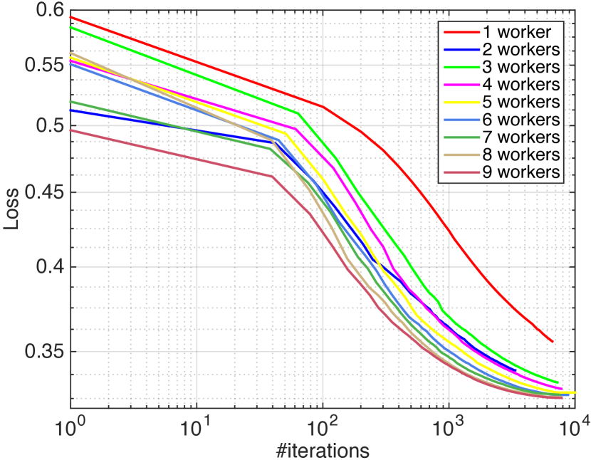
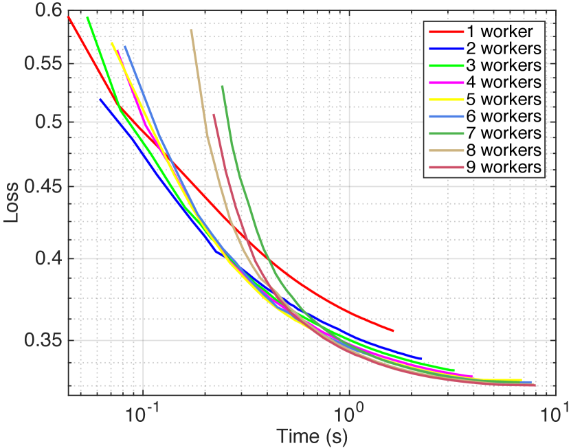
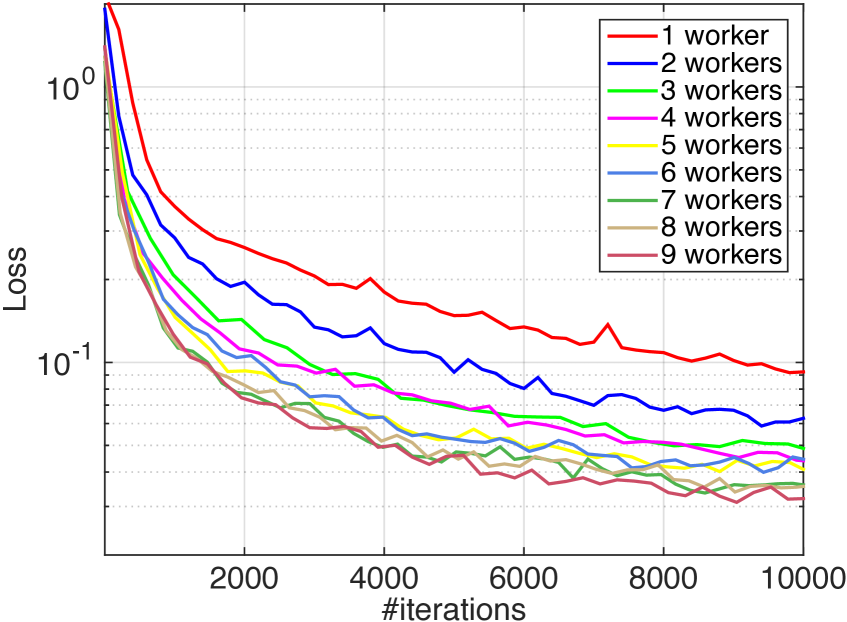
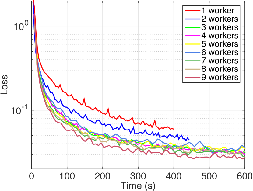
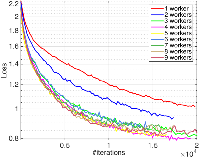
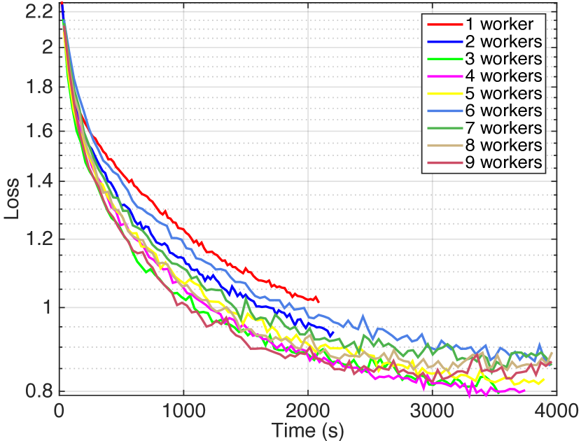
Figure 6: Testing loss vs. #workers. From top down, each row corresponds to the a9a, MNIST and CIFAR dataset, respectively.

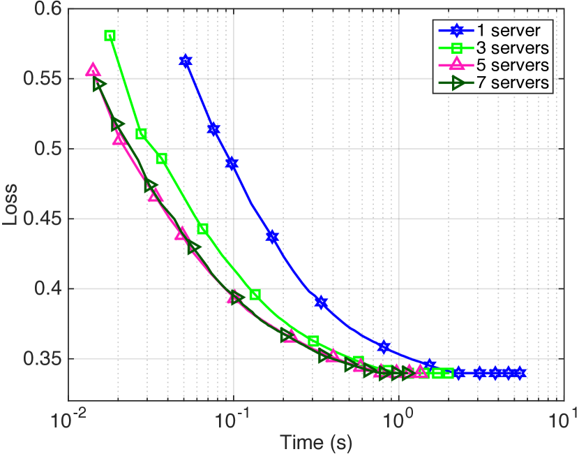
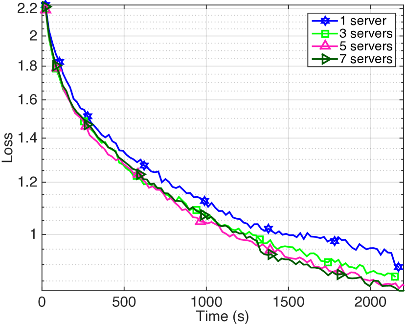
Figure 7: Testing loss vs. #servers. From left to right, the first row corresponds to the a9a, MNIST datasets, and the second row corresponds to the CIFAR dataset, respectively.

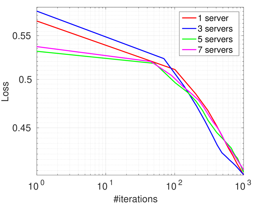
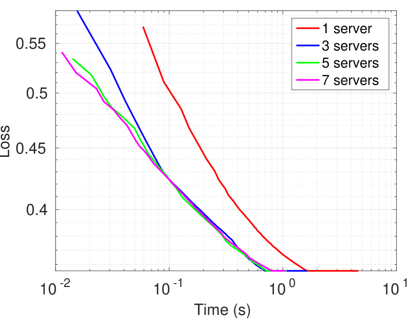
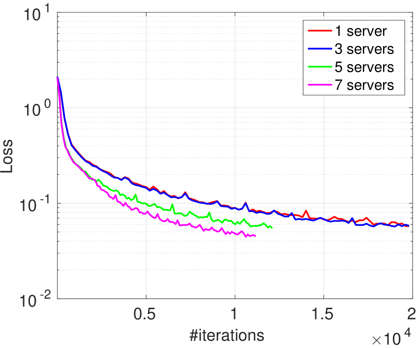
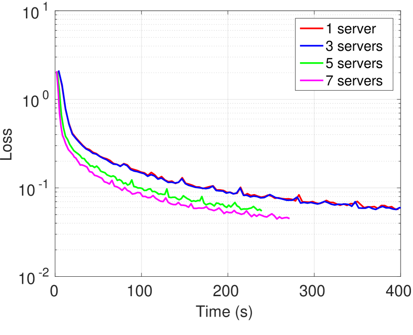
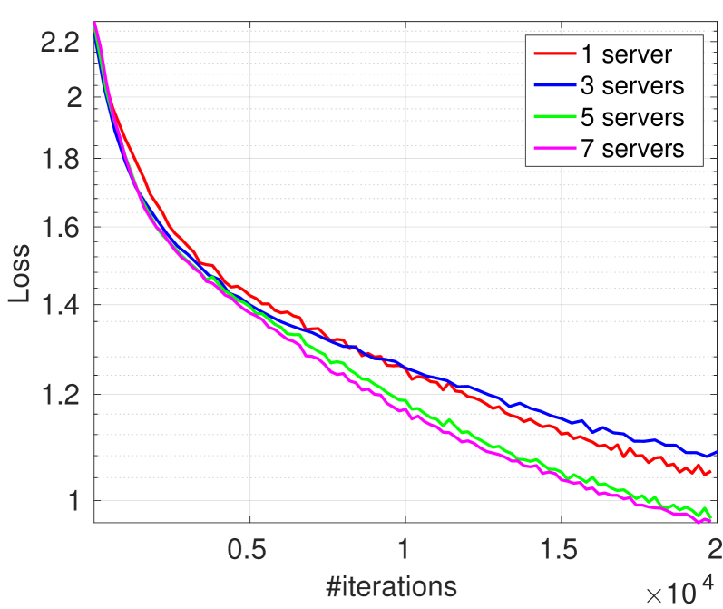
Figure 8: Testing loss vs. #servers. From top down, each row corresponds to the a9a, MNIST and CIFAR dataset, respectively. Each server is associated with 1 worker.

Figure 9: Testing loss vs. #servers. From top down, each row corresponds to the a9a, MNIST and CIFAR dataset, respectively. Each server is associated with 2 workers.

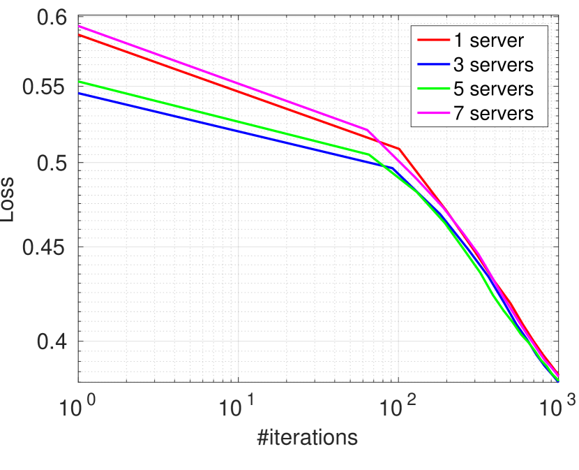
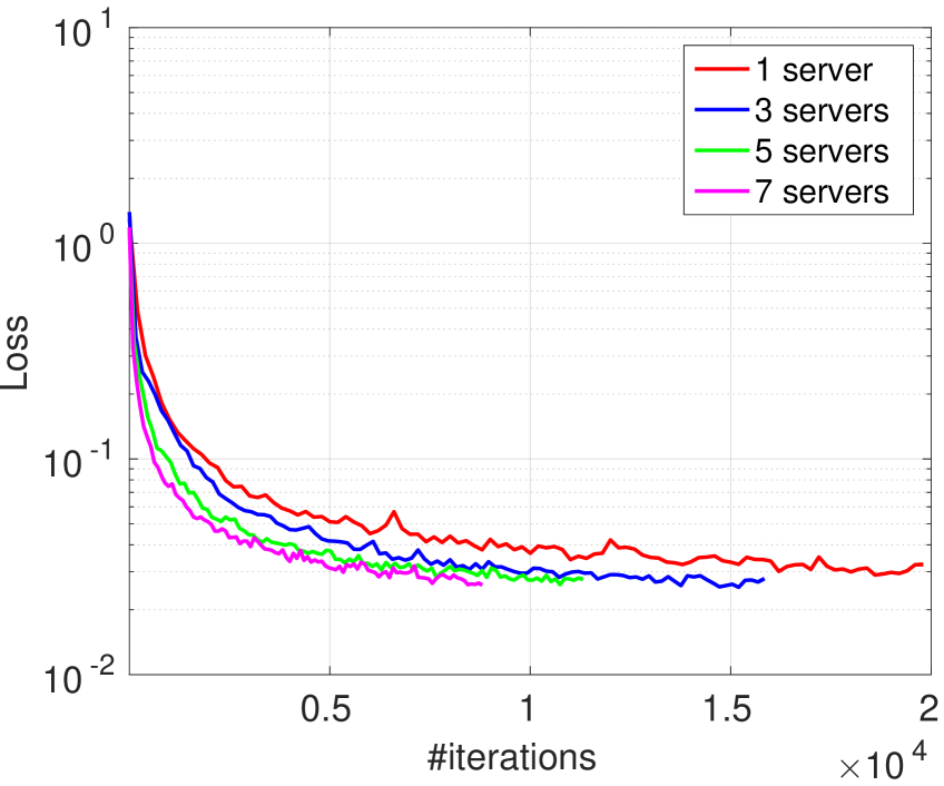
Figure 10: Testing loss vs. #servers. From top down, each row corresponds to the a9a, MNIST and CIFAR dataset, respectively. Each server is associated with 4 workers.

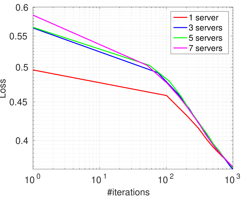
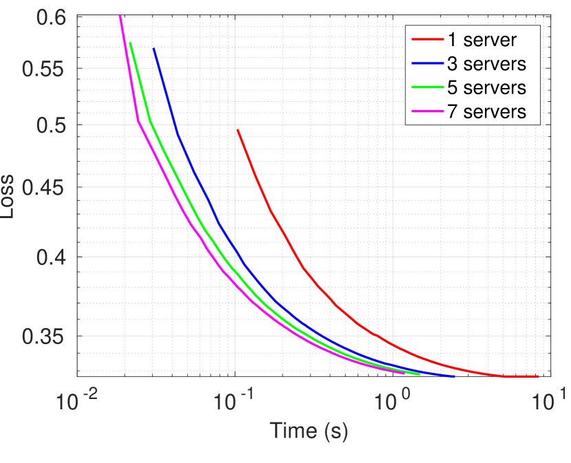
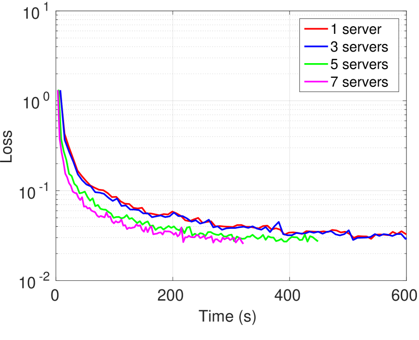
Figure 11: Testing loss vs. #servers. From top down, each row corresponds to the a9a, MNIST and CIFAR dataset, respectively. Each server is associated with 6 workers.

References

• [1] L. Bottou, editor. Online algorithms and stochastic approximations. Cambridge University Press, 1998.
• [2] L. Bottou. Stochastic gradient descent tricks. Technical report, Microsoft Research, Redmond, WA, 2012.
• [3] M. Welling and Y. W. Teh. Bayesian learning via stochastic gradient Langevin dynamics. In ICML, 2011.
• [4] T. Chen, E. B. Fox, and C. Guestrin. Stochastic gradient Hamiltonian Monte Carlo. In ICML, 2014.
• [5] N. Ding, Y. Fang, R. Babbush, C. Chen, R. D. Skeel, and H. Neven. Bayesian sampling using stochastic gradient thermostats. In NIPS, 2014.
• [6] A. Agarwal and J. C. Duchi. Distributed delayed stochastic optimization. In NIPS, 2011.
• [7] J. Dean et al. Large scale distributed deep networks. In NIPS, 2012.
• [8] T. Chen et al. MXNet: A flexible and efficient machine learning library for heterogeneous distributed systems. (arXiv:1512.01274), Dec. 2015.
• [9] M. Abadi et al. TensorFlow: Large-scale machine learning on heterogeneous systems, 2015. Software available from tensorflow.org.
• [10] Q. Ho, J. Cipar, H. Cui, J. K. Kim, S. Lee, P. B. Gibbons, G. A. Gibbons, G. R. Ganger, and E. P. Xing. More effective distributed ML via a stale synchronous parallel parameter server. In NIPS, 2013.
• [11] M. Li, D. Andersen, A. Smola, and K. Yu. Communication efficient distributed machine learning with the parameter server. In NIPS, 2014.
• [12] X. Lian, Y. Huang, Y. Li, and J. Liu. Asynchronous parallel stochastic gradient for nonconvex optimization. In NIPS, 2015.
• [13] A. Ahmed, M. Aly, J. Gonzalez, S. Narayanamurthy, and A. J. Smola. Scalable inference in latent variable models. In WSDM, 2012.
• [14] S. Ahn, B. Shahbaba, and M. Welling. Distributed stochastic gradient MCMC. In ICML, 2014.
• [15] S. Ahn, A. Korattikara, N. Liu, S. Rajan, and M. Welling. Large-scale distributed Bayesian matrix factorization using stochastic gradient MCMC. In KDD, 2015.
• [16] U. Simsekli, H. Koptagel, Guldas H, A. Y. Cemgil, F. Oztoprak, and S. Birbil. Parallel stochastic gradient Markov chain Monte Carlo for matrix factorisation models. Technical report, 2015.
• [17] C. Chen, N. Ding, and L. Carin. On the convergence of stochastic gradient MCMC algorithms with high-order integrators. In NIPS, 2015.
• [18] F. Niu, B. Recht, C. Ré, and S. J. Wright. Hogwild!: A lock-free approach to parallelizing stochastic gradient descent. In NIPS, 2011.
• [19] H. R. Feyzmahdavian, A. Aytekin, and M. Johansson. An asynchronous mini-batch algorithm for regularised stochastic optimization. Technical Report arXiv:1505.04824, May 2015.
• [20] S. Chaturapruek, J. C. Duchi, and C. Ré. Asynchronous stochastic convex optimization: the noise is in the noise and SGD don’t care. In NIPS, 2015.
• [21] S. L. Scott, A. W. Blocker, and F. V. Bonassi. Bayes and big data: The consensus Monte Carlo algorithm. Bayes 250, 2013.
• [22] M. Rabinovich, E. Angelino, and M. I. Jordan. Variational consensus Monte Carlo. In NIPS, 2015.
• [23] W. Neiswanger, C. Wang, and E. P. Xing. Asymptotically exact, embarrassingly parallel MCMC. In UAI, 2014.
• [24] X. Wang, F. Guo, K. Heller, and D. Dunson. Parallelizing MCMC with random partition trees. In NIPS, 2015.
• [25] J. C. Mattingly, A. M. Stuart, and M. V. Tretyakov. Construction of numerical time-average and stationary measures via Poisson equations. SIAM Journal on Numerical Analysis, 48(2):552–577, 2010.
• [26] Y. A. Ma, T. Chen, and E. B. Fox. A complete recipe for stochastic gradient MCMC. In NIPS, 2015.
• [27] S. Patterson and Y. W. Teh. Stochastic gradient Riemannian Langevin dynamics on the probability simplex. In NIPS, 2013.
• [28] C. Li, C. Chen, D. Carlson, and L. Carin. Preconditioned stochastic gradient Langevin dynamics for deep neural networks. In AAAI, 2016.
• [29] S. Zhang, A. E. Choromanska, and Y. Lecun. Deep learning with elastic averaging SGD. In NIPS, 2015.
• [30] Y. W. Teh, L. Hasenclever, T. Lienart, S. Vollmer, S. Webb, B. Lakshminarayanan, and C. Blundell. Distributed Bayesian learning with stochastic natural-gradient expectation propagation and the posterior server. Technical Report arXiv:1512.09327v1, December 2015.
• [31] R. Bardenet, A. Doucet, and C. Holmes. On Markov chain Monte Carlo methods for tall data. Technical Report arXiv:1505.02827, May 2015.
• [32] T. Jia, E. Shelhamer, J. Donahue, S. Karayev, J. Long, R. Girshick, S. Guadarrama, and T. Darrell. Caffe: Convolutional architecture for fast feature embedding. arXiv preprint arXiv:1408.5093, 2014.
• [33] C. Blundell, J. Cornebise, K. Kavukcuoglu, and D. Wierstra. Weight uncertainty in neural networks. In ICML, 2015.
• [34] A. Krizhevshy, I. Sutskever, and G. E. Hinton. Imagenet classification with deep convolutional neural networks. In NIPS, 2012.
• [35] S. J. Vollmer, K. C. Zygalakis, and Y. W. Teh. (Non-)asymptotic properties of stochastic gradient Langevin dynamics. Technical Report arXiv:1501.00438, University of Oxford, UK, January 2015.