Three phase classification of an uninterrupted traffic flow: a $k$-means clustering study

Abstract

We investigate the speed time series of the vehicles recorded by a camera at a section of a highway in the city of Isfahan, Iran. Using $k$-means clustering algorithm, we find that the natural number of clustering for this set of data is $3$. This is in agreement with the three-phase theory of uninterrupted traffic flows. According to this theory, the three traffic phases are categorized as free flow (F), synchronized (S) and wide moving jam (J). We obtain the transition speeds and densities at F-S and also S-J transitions. We also apply the Shannon entropy analysis on the speed time series over finite windows, which equips us to monitor in areal time the instant state of a traffic flow.

I Introduction

Understanding the nature of traffic congestion and the mechanism of its formation in uninterrupted facilities enlightens the traffic science and paves the way for more accurate short term forecasting and traffic management and control Raj ; golob . Various analytical models proposed in this regard could be categorized in two paradigms. The first is based on fundamental diagrams (Lighthill and Whitham 1955 Lighthill , Richards 1956 Richards , Daganzo 1994Daganzo4 , 1995Daganzo5 , Tang et al. 2012 Tang ) and the second is based on driver reaction characteristics (Chandler et al. 1958 Chandler58 , Gazis et al. 1961Gazis , Gipps 1981Gipps , Krau$\beta$ 1998Krau , Aw and Rascle 2000 Rascle , Newell 2002 Newell , Kesting and Treiber 2008Kesting ).

The classical traffic theory distinguishes between two phases of traffic stream namely free and congested flow. Accordingly, the flow-density space i.e. fundamental diagram is assumed to consist of two sub-spaces. The quest for theories capable of better explaining the critical features such as traffic breakdown (onset of congestion in an initial free flow) yielded the development of the three phase traffic theory Kerner2 ; Kerner3 ; Kerner4 ; kerner . Since its emergence, the three-phase theory has been noticeably applied in traffic analysis. Hausken and Rehborn (2015)Hausken started extending the three-phase theory into the game theoretic domain. Jia et al. (2011)Jia proposed a cellular automaton model with time gap dependent randomization under the three-phase traffic theory. Tian (2012)Tian proposed average space gap model (ASGM) - a cellular automaton for traffic flow within the fundamental diagram - which could reproduce aspects of the three-phase theory. Some empirical examples of the validation of the traffic phase can be found in Rehnborn et al. (2011)rehborn and Schäfer et al. (2011)schafer .

According to Schönhof and Helbing (2009)Helbing , a major shortcoming of the three-phase theory is its vagueness in defining the boundaries of congested phases i.e. S and J. Therefore, this paper tries to develop a framework for distinguishing three phases without having to consider too many criteria.

In this work we employ a specific clustering scheme, the so called $k$-means clustering algorithm, for classification of different phases of an uninterrupted traffic flow. Data for this research came from automatic speed detectors installed in urban highways of Isfahan, Iran.

The rest of the paper is organized as follows. In section  II a brief introduction of the three phase traffic theory is presented. In section III the methodology used in our data analysis is introduced. section IV gives some details related to the recorded speed data. Sections V and VI discuss the results of applying $k$-means clustering method and also Shannon entropy on the speed time series, respectively. Section VII is devoted to the conclusion.

II The Three-Phase Traffic Theory

Three-phase traffic theory assumes free flow (F), synchronized flow (S) and wide moving jam (J) for traffic stream. Actually, under three-phase formalism, classical congested traffic is divided into two distinct phases named as synchronized flow and wide moving jam. F is the state in which because of the low density of traffic, the interactions among vehicles are negligible and vehicles move at their desired speed. S is the state in which speed is synchronized within and among lanes and there is a continuous flow with no significant stopping and low probability of passing which results in bunching of vehicles (a tendency towards synchronization of vehicle speeds in each of the road lanes). J is the state in which a jam moves upstream through any highway bottlenecks, maintaining the mean speed of the downstream front. The difference of a wide and a narrow moving jam lays in maintaining the mean speed of the downstream jam front Hausken .

By establishing three traffic phases, three phase transitions may be imagined (F$\rightarrow$S, S$\rightarrow$J, F$\rightarrow$J) among which the theory rejects the possibility of F$\rightarrow$J. Therefore, free-flow state transits to wide moving jam only through synchronized state. The phase transition F$\rightarrow$S at a bottleneck can be explained by a competition between over-acceleration and speed adaptation. The lane changing behavior exhibits dual roles in phase transitions. The lane changing behavior that causes a strong reduction in following vehicle speeds in the target lane is responsible for the phase transition F$\rightarrow$S or S$\rightarrow$J. In contrast, lane changing to a faster lane can lead to the phase transition S$\rightarrow$F or J$\rightarrow$S (Kerner and Klenov, 2009kerner ). Based on three-phase theory, traffic breakdown (F$\rightarrow$S transition) occurs if two conditions are satisfied. First, the flow rate in free flow downstream ($q$) of a bottleneck lies between a threshold flow rate for traffic breakdown at the bottleneck ($q_{th}^{\bf B}$) and the maximum flow rate in free flow downstream of the bottleneck ($q_{\bf max}^{\bf freeB}$). Second, a nucleus, required for traffic breakdown, appears in free flow at the bottleneck. A nucleus is a local disturbance in free flow within which the vehicle speed is equal or lower than the critical speed or the vehicle density is equal to or greater than the critical density required for the traffic breakdown. This implies that there is infinite number of flow rates in free flow downstream of the bottleneck for which traffic breakdown at the bottleneck is possible.

It is possible to define an empirical minimum velocity ($V_{\rm min}^{\rm free,emp}$) which separates the free flow from the synchronized flow as

$$V_{\rm min}^{\rm free,emp}=q_{\rm max}^{\rm free,emp}/D_{\rm max}^{\rm free,emp},$$ (1)

which implies that at the limiting (maximum) point of free flow, the density and flow rate reach their maximum values denoted by $D_{\rm max}^{\rm free,emp}$ and $q_{\rm max}^{\rm free,emp}$, respectively. At F state, speeds are greater and at S and J speeds are less than $V_{\rm min}^{\rm free,emp}$ Kerner2 ; Kerner3 . One can show all these information in the fundamental diagram but there is no specified region to separate S state from J state in this diagram. Three-phase theory gives a wide region in which transition from S$\rightarrow$J is possible.

To distinguish between S and J, a parameter $I={\tau_{J}}/{\tau^{(a)}_{\rm del,jam}}$ is defined where $\tau_{J}$ is the duration of a wide moving jam and $\tau^{(a)}_{\rm del,jam}$ is the mean time in vehicle acceleration at the downstream front of a wide moving jam. Whenever $I\gg 1$ and a nucleus appears, the S$\rightarrow$J transition takes place. Although clear, this definition is not easy to use. Calculating parameter $\tau_{J}$ is not easy and also one needs continuous online observation of the highway to check the creation of nucleus.

III Methodology

Data analysis is a process of obtaining useful information from raw data. For this purpose, statistical methods are the natural toolsjudd . In this work, we use the $k$-means clustering algorithm and Shannon entropy to verify the three-phase states in an uninterrupted traffic flow.

III.1 $k$-means clustering

We use $k$-means clusterings method to determine the different states of traffic flow. $k$-means algorithm is widely used in data mining for partitioning of $n$ measured quantities into $k$ clusters James ; Hartigan .

In this method, a given set of measurements $(x_{1},x_{2},\dots,x_{n})$, can be grouped in $k$ clusters by minimizing the within-cluster sum of squares (WCSS), i.e $\min_{S}\sum_{i=1}^{k}\sum_{x\in S_{i}}||x-\mu_{i}||^{2}$, in which $\mu_{i}$ is the mean of variables in the cluster $S_{i}$.

The quality and naturalness of the clustering in $k$-means method can be evaluated by Silhouettes analysis Hennig ; silhouettes . Silhouettes coefficient is defined as

$$S(i)=\frac{b(i)-a(i)}{\max{(b(i),a(i))}},$$ (2)

where $a(i)$ is the average distance from one data to all other data within the same cluster and $b(i)$ is the average distance of the data to the nearest cluster of its own assigned cluster. $S_{i}$ varies from $-1$ to $+1$, where a high positive (negative) value indicates that the data is a well (poorly) clustered. In the case of highly negative $S_{i}$ one needs to move the data to the neighboring cluster. When $S(i)$ is close to zero, object i can be considered to be in both clusters.

After finding $S(i)$ for each node, one can find the average Silhouettes coefficient for all the data. The best number of clusters, known as natural cluster numbering of that data, is the one with the biggest average Silhouettes coefficient  Hennig .

III.2 Shannon Entropy

To distinguish the different traffic states, we also use the Shannon entropy as a measure of information content of the speed time series. Entropy has important physical implications as the amount of ”disorder” in a system shannon . Shannon Entropy is used in different branches of science such as the structure of ecosystems Masahiko , security valuation in finance Stutzer ; Lillo and also in Seismology Beenamol .

The Shannon entropy corresponding to the stochastic variable is defined as

$$H=-\sum_{i}p(x_{i})\log_{2}(p(x_{i})),$$ (3)

where $p(x_{i})$ is the probability that $X$ takes the value $x_{i}$.

In an ordered state for which $p(x_{n})=1$ and $p(x_{i})=0$ for any $i\neq n$ the Shanon entropy vanishes. The entropy is maximum if all the states have the same probability which is equivalent to the maximum information contained in the system.

IV Data Set

Our data set is collected from a section of Sayyad highway in Isfahan, Iran. Our database contains the speed of vehicles (in the unit of km/h), collected in $5$ days: $8-10-2014$, $9-10-2014$ (weekend), $10-10-2015$ (weekend), $11-10-2015$ and $12-10-2015$. Recording limits are $5$ and $119$ km/h with the precision of $1$ km/h.

Figures 1-a,b,c,d,e demonstrates the speed time series during these $5$ days. Figure 2 shows the histogram of cumulative speed time series for all the $5$ days. It can be seen from this figure that there is a large peak in the speed histogram at $v\sim 75$ km/h, corresponding the free flow, and also a small peak corresponding to the wide moving jam at $v\sim 20$ km/h.

Figure 3 exhibits the scatter plot of the speed at any two successive times $t+1$ versus $t$ (top panel) and also the conditional probability of finding speed at the value $v_{2}$ at time $t+1$ provided that its value at time $t$ be $v_{1}$ (bottom panel).

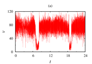
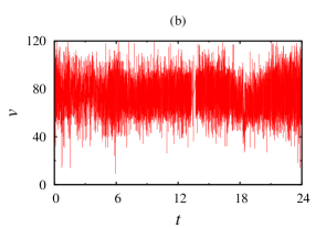
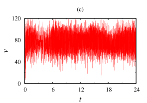
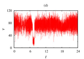
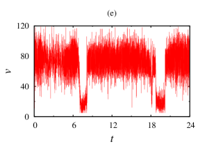
Figure 1: (Color online) Vehicle speed data at a cross section of Sayyad highway in Isfahan for the days (a) $8-10-2014$, (b) $9-10-2014$ (weekend), (c) $10-10-2015$ (weekend), (d) $11-10-2015$ and (e) $12-10-2015$.

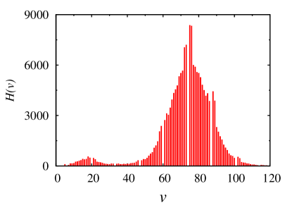
Figure 2: (Color online) Speed histogram for $5$ days of recorded data.

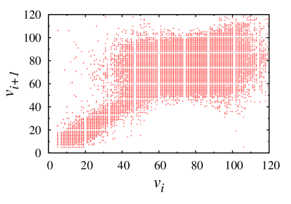
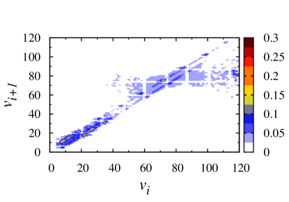
Figure 3: (Color online) (Top): Scatter plot of speed at successive times, $v_{i+1}$ versus $v_{i}$. (Bottom): The density plot of the conditional probability $p(v_{2},i+1|v_{1},i)$.

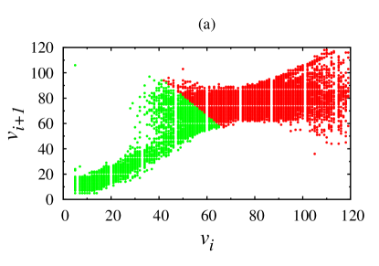
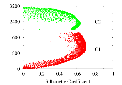
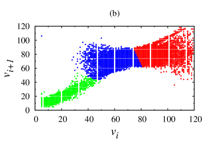
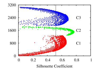
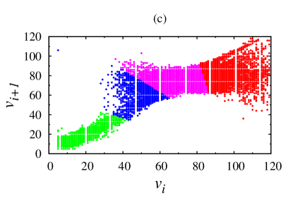
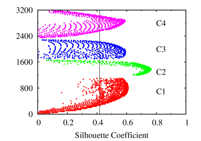
Figure 4: (Color online) (Left) $k$-means clustering of data into (a) $2$, (b) $3$ and (c) $4$ clusters. (Right) Silhouette coefficient for (a) $2$, (b) $3$ and (c) $4$ clusterings.

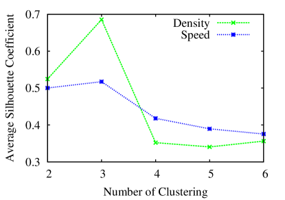
Figure 5: (Color online) The average of Silhouette coefficients for different clustering numbers for scatter plot of speed (bluet) and density (green) time seires.

V clustering of vehicle speed time series

In order to use the $k$-means method for data clustering, first we assume a specific number of clusters and obtain the corresponding Silhouette coefficient, then to obtain the natural number of clusters, we find the clustering for which the Silhouette coefficient is maximum. In this work, we apply $k$-means algorithm to the scatter plot of speed data ($v_{i+1}$ versus $v_{i}$), shown in figure 3. To reduce the highly rare events which may results in unreal clustering, we first eliminate the data of the scatter plot with low conditional probability, say $p(v2,i+1|v1,i)<0.001$. Results of clustering data to $2$, $3$ and $4$ groups are shown in the right panel of figures 4-(a), (b) and (c), respectively. The Silhouette coefficients calculated for data in each clustering are also illustrated in the left panel of figures 4-(a), (b) and (c). The vertical lines in silhouette plots, show the average silhouette coefficient for that clustering.

The average Silhouette coefficient corresponding to different number of clustering are represented in figure 5 (blue symbols), showing this average reaches to a maximum at $N=3$, whose message is that the natural number of clustering is $3$.

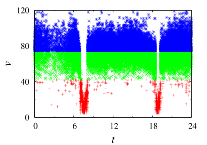
Figure 6: (Color online) $k$-means clustering of one day speed time series into $3$ clusters.

We also apply $k$-means method for clustering of the speed time series itself into three groups. As the results of such a clustering (shown in figure 6 for the first day) we find three groups: (i) $0\leq v\lesssim 42$ km/h for wide moving jam, (ii) $43$ km/h $\lesssim v\lesssim 74$ km/h for the synchronized phase and (iii) $74$ km/h $\lesssim v\lesssim 120$ km/h for the free flow.

It is also possible to obtain a rough estimation of density from the speed time series. Consider a time window in the speed series of length $N$ vehicles, starting from the time $t_{i}$. Then the density at the time $t_{i}$ ($D_{i}$) can be estimated as

$$D_{i}=\frac{N}{\Delta t_{i}\bar{V}_{i}},$$ (4)

in which $\Delta t_{i}$ denotes the time duration of passing $N$ vehicles starting from the time $t_{i}$, and ${\bar{V}}_{i}$ is the average speed of the vehicles in this window. Here we choose the window of $N=50$. Figure 7 represents the density times series for one day of the highway traffic flow, in which the wide moving jams appear as sharp peaks.

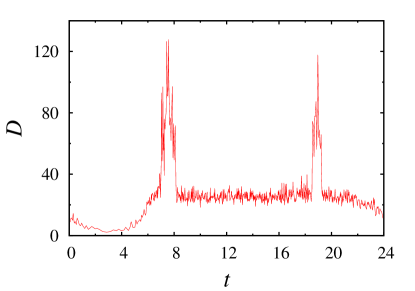
Figure 7: (Color online) Vehicle density time series for the day 9-10-2014 corresponding to the speed time series shown in Fig 1-(a).

Figure 8 shows the results of the implementation of $k$-means clustering method on the density scatter plot for successive time windows ($D_{i+1}$ vs $D_{i}$) into three clusters. The silhouette analysis, (figure 5, green symbols), again reveals $3$ natural clustering for the uninterrupted traffic flow. As it makes us sure that three clustering is the best natural number of clusters for density, we can find the values of the densities separating those three regions by simply applying the three clustering $k$-means on the density time series. The results are exhibited in figure 9 and show that the three groups of density can be classified as (i) $0\leq D\lesssim 18$/km for free flow, (ii) $18$/km$\lesssim D\lesssim 50$/km for the synchronized phase and (iii) $D>50$/km for the wide moving jam.

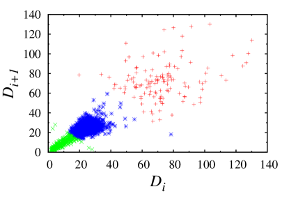
Figure 8: (Color online) $k$-means clustering clustering for $k=3$ on density scatter plot.

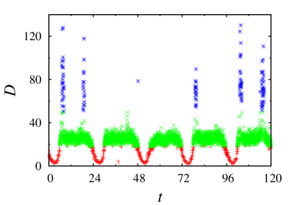
Figure 9: (Color online) $k$-means clustering clustering for k=3 on density series.

To wrap up this section, we discuss the fundamental diagram of speed versus density illustrated in figure 10. The three phases of the uninterrupted traffic flow are also apparent in this figure. It can be seen that the free flow and wide moving jam can be identified by the region in the fundamental diagram ($v-D$), where speed is roughly a constant value independent of density. In this case, for the density less than $\sim 18$/km (free flow) the average speed of the vehicles is about $75$ km/h, while for vehicle density larger than $\sim 50$/km (wide moving jam) the average speed is roughly $20$ km/h. Between these two limits (synchronized) the average speed decreases almost linearly with increasing density.

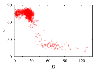
Figure 10: (Color online) Fundamental diagram of speed versus density.

VI Shannon Entropy analysis of speed time series

In this section, we employ the Shannon entropy analysis to extract information contained in the time series. Thanks to $k$-means clustering method which gives us the boarder values of speed separating the three traffic phases, the information of the time series coming from each state can be calculated as

$$H_{J}=-\Sigma_{v=0}^{v_{j}}p(v)\log p(v)$$

$$H_{S}=-\Sigma_{v=v_{j}}^{v_{s}}p(v)\log p(v)$$

$$H_{F}=-\Sigma_{v=v_{s}}^{v_{m}}p(v)\log p(v),$$ (5)

where $p(v)$ is the probability of finding speed in the interval $[v,v+1]$ and $H_{J}$, $H_{S}$ and $H_{F}$ denote the Shannon entropy corresponding to wide moving jam, synchronized and free flow, respectively. $v_{s}$ is the transition speed separating wide moving jam from synchronized, $v_{j}$ is the speed at the border of synchronized and free flow states and $v_{m}=120$ km/h is maximum recored speed. Based on $k$-means clustering analysis we set $v_{j}=42$ km/h and $v_{s}=74$ km/h.

We are interested in determining the instant state of traffic flow, hence we first divide the time series into the finite time windows of the order of correlation length of time series which is typically $50$. In figure 11 the three entropies are plotted close to the occurrence of a wide moving jam. This figure clearly shows the transition between different phases of traffic. As can be seen in figure 11, long before the jam the dominant entropy is $H_{F}$, an indication of free flow phase, however before the onset of jam, synchronized entropy $H_{S}$ rises and become dominant over the other two and finally at the onset of jamming it is the wide moving jam entropy $H_{j}$ which acquires the largest value. Right after the end of jamming state, however, none of the synchronized or free flow entropies are dominant over each other, meaning that during time periods right after the end of the jamming phase, there could be coexistence between F and S phases.

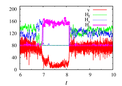
Figure 11: (Color online) Shannon entropies corresponding to wide moving jam ($H_{J}$), synchronized ($H_{S}$) and free flow ($H_{F}$) states of speed time series around a wide moving jam. For better visualization, the entropies are multiplied by the factor $3$.

VII conclusion

In summary, we found that $k$-means clustering method is a powerful instrument to characterize different states of an uninterrupted traffic flow. Applying this method to both the speed times series and also the density time series calculated form speed data, we sound that the three phases wide moving jam, synchronized and free flow come up as the natural clusters. This method gives us the speed and densities at which the transitions between these states occur. Implementation of Shannon entropy analysis over finite time windows, enabled us to find the short time states of traffic flow. From the Shannon entropy analysis we find that in going from free flow to a wide moving jam, first a transition occurs between the F and S and then from S to J. Nevertheless, right after the end of a wide moving jam, synchronized and free flow states could coexists.

Our findings in this work are consistent with three-phase theory and we hope that may open avenues through optimization for highwy traffic programming.

References

- (1) Jain, R. (1996). Congestion control and traffic management in ATM networks: Recent advances and a survey. Computer Networks and ISDN systems, 28(13), 1723-1738.
- (2) Golob, T. F., Recker, W. W. (2003). Relationships Among Urban Freeway Accidents, Traffic Flow, Weather, and Lighting Conditions. Journal of transportation engineering, 129(4), 342-353.
- (3) Lighthill, M. J., Whitham, G. B. (1955). On kinematic waves: A theory of traffic flow on long crowded roads. Proc. R. Soc. A, Math. Phys. Eng. Sci., 229, 281–345.
- (4) Richards, P. I. (1956). Shockwaves on the highway. Oper. Res., 4, 42–51.
- (5) Daganzo, C. F. (1994). The cell transmission model: a simple dynamic representation of highway traffic. Transp. Res., Part E, Logist. Transp. Rev., 28, 269–287.
- (6) Daganzo, C. F. (1995). The cell transmission model, part II: network traffic. Transp. Res., Part B, Methodol., 29, 79–93.
- (7) Tang, T., Li, C., Huang, H. and Shang, H. (2012). A new fundamental diagram theory with the individual difference of the driver’s perception ability. Nonlinear Dynamics, 67(3), pp.2255-2265.
- (8) Chandler, R.E., Herman, R., Montroll, E.W. (1958). Traffic dynamics: studies in car following. Operational Research, 6:165–184.
- (9) Gazis, D.C., Herman, R., Rothery, R.W. (1961). Nonlinear follow-the-leader models of traffic flow. Operational Research, 9.
- (10) Gipps, P.G. (1981). A behavioral car-following model for computer simulation. Transportation Research Part B: Methodological, 15(2), pp.105-111.
- (11) Krau, S. (1998). Microscopic modeling of traffic flow: Investigation of collision free vehicle dynamics. (Doctoral dissertation, Universitat zu Koln.)
- (12) Aw, A. and Rascle, M. (2000). Resurrection of” second order” models of traffic flow. SIAM journal on applied mathematics, 60(3), pp.916-938.
- (13) Newell, G.F. (2002). A simplified car-following theory: a lower order model. Transportation Research Part B: Methodological, 36(3), pp.195-205.
- (14) Kesting, A. Treiber, M. (2008). How reaction time, update time, and adaptation time influence the stability of traffic flow. Computer‐Aided Civil and Infrastructure Engineering, 23(2), pp.125-137.
- (15) Kerner, B.S. (1999). The physics of traffic. Physics World Magazine 12, 25-30.
- (16) Kerner, B.S. (1999). Congested Traffic Flow: Observations and Theory. Transportation Research Record, Vol. 1678, pp. 160-167.
- (17) Kerner, B.S. (2004). The Physics of Traffic. Springer, Berlin, New York.
- (18) Kerner, B.S. (2009). Introduction to Modern Traffic Flow, Theory and Control. Springer.
- (19) Hausken, K., and Hubert R. (2015). Game-Theoretic Context and Interpretation of Kerner’s Three-Phase Traffic Theory. Game Theoretic Analysis of Congestion, Safety and Security. Springer International Publishing, 113-141.
- (20) Jia, B., Li, X.G., Chen, T., Jiang, R. and Gao, Z.Y. (2011). Cellular automaton model with time gap dependent randomisation under Kerner’s three-phase traffic theory. Transportmetrica, 7(2), pp.127-140.
- (21) Tian, J.F., Yuan, Z.Z., Treiber, M., Jia, B. and Zhang, W.Y. (2012). Cellular automaton model within the fundamental-diagram approach reproducing some findings of the three-phase theory. Physica A: Statistical Mechanics and its Applications, 391(11), pp.3129-3139.
- (22) Rehborn, H., Klenov, S. L., Palmer, J. (2011). An empirical study of common traffic congestion features based on traffic data measured in the USA, the UK, and Germany. Physica A: Statistical Mechanics and its Applications, 390(23), 4466-4485.
- (23) Schäfer, R. P., Lorkowski, S., Witte, N., Palmer, J., Rehborn, H., Kerner, B. S. (2011) A study of TomTom’s probe vehicle data with three-phase traffic theory. Traffic Engineering Control, 52(5).
- (24) Schönhof, M. and Helbing, D. (2009). Criticism of three-phase traffic theory. Transportation Research Part B: Methodological, 43(7), pp.784-797.
- (25) Judd, C. M., McClelland, G. H., Ryan, C. S. (2011). Data Analysis: A model comparison approach. Routledge.
- (26) MacQueen, J. (1967). Some methods for classification and analysis of multivariate observations. In Proceedings of the fifth Berkeley symposium on mathematical statistics and probability (Vol. 1, No. 14, pp. 281-297).
- (27) Hartigan, J. A. (1975). Clustering Algorithms, New York: John Willey and Sons. Inc. Pages113129.
- (28) de Amorim, R. C., Hennig, C. (2015). Recovering the number of clusters in data sets with noise features using feature rescaling factors. Information Sciences, 324, 126-145.
- (29) Rousseeuw, P. J. (1987). Silhouettes: a Graphical Aid to the Interpretation and Validation of Cluster Analysis. Journal of computational and applied mathematics, 20, 53-65.
- (30) Ellis, R. S. (2012). Entropy, Large Deviations, and Statistical Mechanics. (Vol. 271). Springer Science Business Media.
- (31) Higashi, M. (1986). Extended input-output flow analysis of ecosystems. Ecological Modelling, 32(1-3), 137-147.
- (32) Stutzer, M. (1996). A simple nonparametric approach to derivative security valuation. The Journal of Finance, 51(5), 1633-1652.
- (33) Lillo, F., Farmer, J. D. (2004). The Long Memory of the Efficient Market. Studies in nonlinear dynamics econometrics, 8(3).
- (34) Beenamol, M., Prabavathy, S., Mohanalin, J. (2012). Wavelet based seismic signal de-noising using Shannon and Tsallis entropy. Computers Mathematics with Applications, 64(11), 3580-3593.