Assessment of the Information Content of the Power Spectrum and Bispectrum
Abstract
The covariance matrix of the matter and halo power spectrum and bispectrum are studied. Using a large suite of simulations, we find that the non-Gaussianity in the covariance is significant already at mildly nonlinear scales. We compute the leading disconnected non-Gaussian correction to the matter bispectrum covariance using perturbation theory, and find that the corrections result in good agreement in the mildly nonlinear regime. The shot noise contribution to the halo power spectrum and bispectrum covariance is computed using the Poisson model, and the model yields decent agreement with simulation results. However, when the shot noise is estimated from the individual realization, which is usually done in reality, we find that the halo covariance is substantially reduced and gets close to the Gaussian covariance. This is because most of the non-Gaussianity in the covariance arises from the fluctuations in the Poisson shot noise. We use the measured non-Gaussian covariance to access the information content of the power spectrum and bispectrum. The signal-to-noise ratio (S/N) of the matter and halo power spectrum levels off in the mildly nonlinear regime, . In the nonlinear regime the S/N of the matter and halo bispectrum increases but much slower than the Gaussian results suggest. We find that both the S/N for power spectrum and bispectrum are overestimated by the Gaussian covariances, but the problem is much more serious for the bispectrum. Because the bispectrum is affected strongly by nonlinearity and shot noise, inclusion of the bispectrum only adds modest amount of S/N compared to that of the power spectrum.
I Introduction
Current large scale structure surveys such as those aiming at measuring the baryonic acoustic oscillations are giving important insights into the physics of the universe Percival et al. (2001); Tegmark et al. (2004); Eisenstein et al. (2005); Cole et al. (2005); Tegmark et al. (2006); Anderson et al. (2014). Future surveys such as Euclid Laureijs et al. (2011) and LSST LSST Science Collaboration et al. (2009) will measure the large scale structure over a large volume and in deep redshift ranges with unprecedented precision. To correctly interpret the data, the challenge is not only to accurately model the observables, such as the power spectrum and bispectrum, but the covariance matrix of these quantities must also be known with sufficient precision.
The covariance is often measured by running large numbers of mocks, where the survey is modelled starting from a large scale structure simulation. In this approach the mocks not only can take into account the intrinsic correlation, but also the survey geometry and various systematic effects. To get good control of the covariance, often hundreds or even thousands of simulations are required. As it is computationally expensive to run the full -body simulations, various cheap approximate methods are often used (see Ref. Monaco (2016) and references therein for a review of some of the methods that have been proposed).
However, to reach a better understanding and modelling of the covariance it is easier to start with the relatively simpler case of dark matter and halos in -body simulations. This approach has been used to study the covariance of the power spectrum for dark matter Meiksin and White (1999); Scoccimarro et al. (1999); Smith (2009); Takahashi et al. (2011); Harnois-Déraps and Pen (2012); Blot et al. (2015) and halos Smith (2009). For the bispectrum PTHalos Scoccimarro and Sheth (2002) has been used to investigate the covariance systematically Sefusatti et al. (2006); Scoccimarro et al. (2004).
Analytical methods also prove fruitful, as they give interesting insights into what the relevant contributions are for the estimation of the covariance. The dark matter power spectrum has been modelled using perturbation theory Scoccimarro et al. (1999); Bertolini et al. (2016); Mohammed et al. (2016) and halo model Cooray and Hu (2001); Mohammed and Seljak (2014). The Poisson model has been invoked to model the shot noise contribution to the covariance Matarrese et al. (1997); Smith (2009). In particular, by combining the analytical and numerical approaches, it has been realized that beat coupling or supersample covariance can be a significant contribution to the covariance in real surveys Rimes and Hamilton (2006); Hamilton et al. (2006); de Putter et al. (2012); Takada and Hu (2013); Li et al. (2014).
In this paper we study the power spectrum and bispectrum covariance numerically and analytically. Taking advantage of the large suite of simulations available in the DEUS-PUR project, we study the covariance of the dark matter and halo power spectrum and bispectrum. It is worth stressing that this is the first systematic study of the bispectrum covariance using such large number of -body simulations. We also model the covariance and compare the predictions with the numerical results.
As the power spectrum has been well explored and the bispectrum becomes the next frontier in large scale structure, it is crucial to address how much information one can gain by going beyond the 2-point level. Previous work Sefusatti and Scoccimarro (2005) suggested that there is substantial information content in the high-point statistics such as the bispectrum based on the Gaussian covariance approximation. In the context of weak lensing, similar conclusion was found based on Gaussian covariance Takada and Jain (2004); however, when the non-Gaussian covariance is used, the signal to noise (S/N) is substantially reduced, especially for the bispectrum Kayo et al. (2013); Sato and Nishimichi (2013). Armed with the accurate covariance measured from a large suite of simulations, we assess the information loss in the power spectrum and bispectrum due to the correlations that arise in the nonlinear regime.
This paper is organized as follows. In Sec. II, after reviewing the basic theory of the power spectrum covariance for dark matter and halos, we compare the model prediction against the numerical covariance. Sec. III is devoted to the bispectrum covariance. We first lay down the theory of the dark matter and halo bispectrum covariance. We then compare the numerical bispectrum covariance with the theory predictions. The information content of the power spectrum and the bispectrum is assessed by means of the signal-to-noise ratio in Sec. IV. We conclude in Sec. V. We check the probability distribution of the bispectrum estimator in Appendix A. In Appendix B, we show the derivation of some of formulas used in the main text. The shot noise contribution to the halo power spectrum and bispectrum covariance is derived using the Poisson model in Appendix C. In Appendix D, we check the dependence of the signal-to-noise ratio on the binning width.
II Covariance of power spectrum
The covariance of the dark matter power spectrum has been studied quite extensively both numerically Meiksin and White (1999); Scoccimarro et al. (1999); Takahashi et al. (2011); Blot et al. (2015) and theoretically Meiksin and White (1999); Scoccimarro et al. (1999); Bertolini et al. (2016); Mohammed et al. (2016). On the other hand the covariance of the halo power spectrum is relatively less explored, but see Refs. Angulo et al. (2008); Smith (2009). Although the focus of this section is on the covariance of the halo power spectrum, we also present the results for dark matter for comparison. We first review the basic theory of the power spectrum covariance, which paves the way for the bispectrum covariance that we discuss later on.
II.1 Theory of the power spectrum covariance
Here we first review the theory of the covariance matrix of the matter power spectrum, and then we discuss the covariance of the halo power spectrum.
Suppose that the Fourier modes of the density contrast are binned into bands of width in Fourier space. The power spectrum of , , is defined as
| (1) |
where is the Dirac delta function. From the definition, one can construct a power spectrum estimator as (e.g. Feldman et al. (1994); Scoccimarro et al. (1999))
| (2) |
where is the fundamental mode of the box, ( is the size of the simulation box). Note that the integral is done over all the modes that fall into the band of width . is the volume of the spherical shell
| (3) |
The covariance matrix of is defined as
| (4) | |||||
II.1.1 Dark matter
The covariance matrix of the matter power spectrum was first investigated using perturbation theory in Ref. Scoccimarro et al. (1999), and it has been extended to include loop corrections in Refs. Bertolini et al. (2016); Mohammed et al. (2016). Here we limit ourselves to the theory laid down in Ref. Scoccimarro et al. (1999) as it is not the focus of this paper to model the matter power spectrum covariance as accurately as possible.
Plugging Eq. 2 into Eq. 4, for Gaussian , we get the Gaussian covariance of the power spectrum estimator Feldman et al. (1994)
| (5) |
where is the Kronecker delta function that ensures that the Gaussian covariance is diagonal. The Gaussian covariance is inversely proportional to the number of modes in the bin (and it is inversely proportional to the bin width ). For Gaussian field, the power spectrum in Eq. 5 should be the linear one. As we include non-Gaussian corrections below, one of the power spectrum should be the 1-loop one so that it is of the same order as the non-Gaussian results. However, since the 1-loop power spectrum over-predicts the numerical power spectrum already at at , we use the nonlinear power spectrum measured from simulations in place of the 1-loop result.
The non-Gaussian contribution to the power spectrum covariance comes from the trispectrum Meiksin and White (1999); Scoccimarro et al. (1999)
| (6) | |||||
Only the parallelogram shape trispectrum contributes to the power spectrum covariance. The non-Gaussian part does not depend on the bin width . Note that both the Gaussian and non-Gaussian covariance are inversely proportional to the volume of the box (through ). We will see that the same is true for the bispectrum covariance. We can trace back the factor to the Dirac delta function in the definition of the polyspectrum, which arises from the statistical translational invariance of the field. Because of this invariance, the amount of statistics is simply proportional to the volume. On the other hand, when a window function is imposed, the statistical translational invariance is broken. Indeed the supersample covariance term scales differently with volume Takada and Hu (2013).
Nonlinearity induces mode coupling and hence non-Gaussianity. The tree-level dark matter trispectrum has two distinct contributions, and Fry (1984); Scoccimarro et al. (1999)
| (8) |
where cyc. denotes cyclic permutations. is the linear power spectrum, and and are the coupling kernels in standard perturbation theory; see Goroff et al. (1986); Bernardeau et al. (2002).
The and contributions to the covariance matrix are then given by
| (9) | |||||
The resultant covariance matrix contribution reads Scoccimarro et al. (1999)
The contribution to the covariance of the power spectrum can be represented graphically, and the results are shown in Fig. 1. We will apply similar techniques to the bispectrum shortly, and it will be more useful as there are more contributions to the bispectrum covariance. In each diagram two black dots on both sides represent the two ’s in the power spectrum estimator. The legs branching from each dot represent the perturbation theory kernels. We use the wavy line to represent the linear power spectrum, while the additional dot on top means that the 1-loop power spectrum should be used instead. The term in the top-left corner is the Gaussian term, while the others are the non-Gaussian terms. The term gives the contribution, and both and combine to give .

It has also been shown that the large scale mode can modulate the small scale modes to cause the so-called beat coupling or supersample covariance Rimes and Hamilton (2006); Hamilton et al. (2006); de Putter et al. (2012); Takada and Hu (2013); Li et al. (2014). This can be a significant source of covariance at small scales in real surveys. However, it only arises when a window function is imposed such as in real surveys or when sub-parts of a huge simulation are considered. In the simulations with periodic boundary conditions, the wave vectors are sharp and the supersample covariance does not appear. When a window function is present, the wave vectors are broadened and the large scale long modes can contribute. At tree level, there is an extra diagram contributing to the trispectrum in addition to the ones shown in Fig. 1, and this leads to beat coupling at large scales.
II.1.2 Halos
We now turn to the halo power spectrum covariance. In this case, besides the complications due to dark matter nonlinearity and halo biasing, the discrete nature of halos contributes further to stochastic fluctuations. In fact, shot noise is the major source of halo covariance as we will see below. In Appendix C.1 we derive the Poisson shot noise contribution to the covariance matrix of the power spectrum using the Poisson model. In the Poisson model, we assume the point particles are formed by Poisson sampling the underlying continuous field. The Poisson fluctuations give rise to the whole hierarchy of the -point correlations in general. In particular, the connected and disconnected 4-point function contribute to the power spectrum covariance. We refer the readers to the Appendix C.1 for details on the derivation. Here we summarize the key results.
There are both Gaussian and non-Gaussian contributions to the covariance due to Poisson shot noise. The Gaussian shot noise contribution, which can be represented diagrammatically by the two disconnected diagrams in Fig. 24, can be combined with the smooth Gaussian covariance Eq. 5 to be written in a compact form Feldman et al. (1994); Smith (2009)
| (11) |
where is the smooth halo power spectrum and with being the mean number density of halos. 111 The presence of the factor is due to the Fourier convention used in this paper. We can convert the formula to the perhaps more popular convention by replacing by . The non-Gaussian shot noise contribution is given by
| (12) | |||||
where the dots denote the contribution associated with the halo bispectrum and also the smooth trispectrum contributions. See Eq. 79 for the full expression. These terms are due to the connected 4-point function in the Poisson model (Diagrammatically, the three types of terms in Eq. 12 can be represented by the first, second, and fourth diagrams in the third row of Fig. 24). For the halo power spectrum we will not include the shot noise contribution associated with the bispectrum for simplicity because we find that the prediction without bispectrum works reasonably well. A simple estimate suggests that this is small compared to the dominant Gaussian term but not negligible.
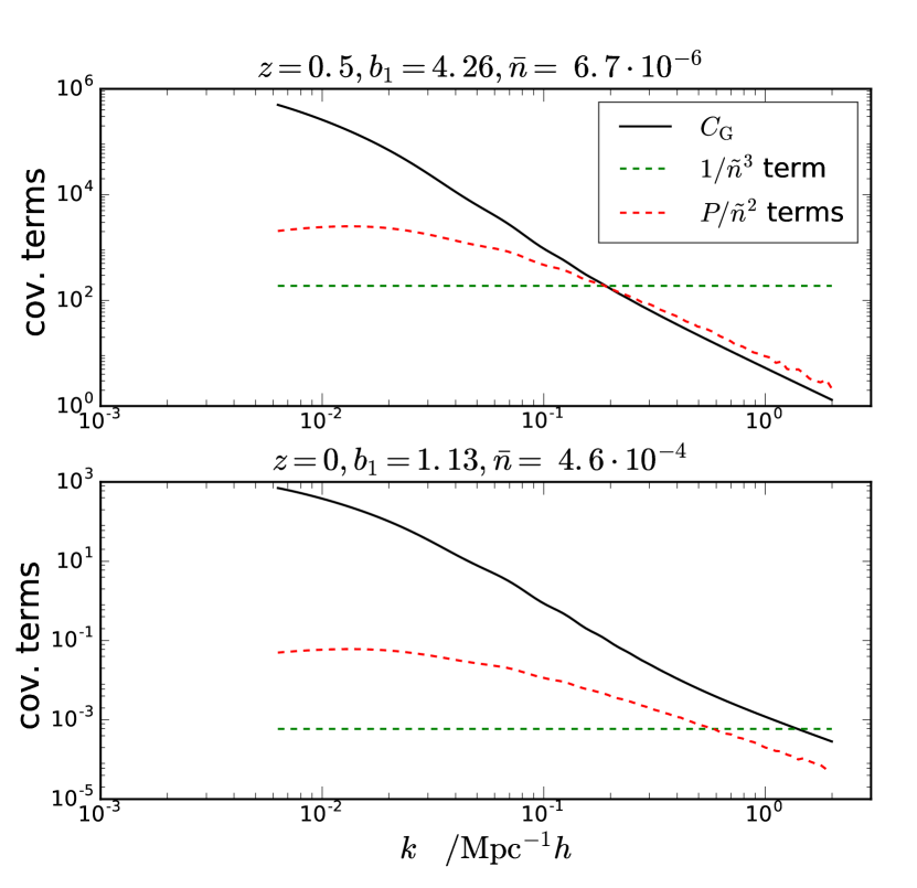
In Fig. 2, we plot the components of the Gaussian and non-Gaussian contributions to the diagonal of the covariance. Note that the covariance depends on the volume of the simulation and the bin width . For the theoretical computations, unless otherwise stated, we use box size , which corresponds to the Small or Hires set shown in Table 1. For the power spectrum, we use the binning width of , which is equal to the fundamental mode of the Small set. We show the results for two representative halo groups, which correpsond to the Large group 4 at and the Hires group 2 at shown in Table 2. We have combined the terms proportional to , which are similar in magnitude. For the low number density group in the range , the Gaussian term, dominates, while for higher , the non-Gaussian term is the only significant term. On the other hand, for the low bias and high number density sample, the Gaussian term is dominant up to .
II.2 Numerical results
In this paper we use the simulations from the DEUS-PUR project Rasera et al. (2014); Blot et al. (2015). We consider three sets of simulations labelled as Large, Small, and Hires respectively. The detailed properties of these simulations are shown in Table 1. A flat CDM model with the WMAP7 cosmological parameters Spergel et al. (2007) is adopted for these simulations. In particular, , , , and . The Zel’dovich approximation is used to generate the Gaussian initial conditions at for the Large and Small sets, and for the Hires set. The transfer function is computed with CAMB Lewis et al. (2000). The simulations are evolved using the adaptive mesh refinement solver RAMSES Teyssier (2002). We consider simulation snapshots at , 0.5, and 0 respectively. The Large and Small sets have the same mass resolution although the box size of the Large set is twice that of the Small set. The Hires has higher mass resolution than the Small set while their box sizes are the same. For more details on the descriptions of the simulations, see Ref. Blot et al. (2015).
The halos used in this work are obtained using the friends-of-friends algorithm with linking length set to 0.2 times the mean inter-particle separation. Only halos with at least 100 particles are used. We divide the halos into four mass groups. The details of these mass groups are shown in Table 2. The simulations of the Large and Small sets only have the highest mass group, Gr. 4, while the Hires set has groups 1, 2, 3, and 4. Moreover, the results at , 0.5 and, 0 are available for the Large and Small sets, while only ones are available for the Hires set. We note that the number density of the halo groups considered here is low compared to the expected number density in future galaxy surveys, e.g. the number density in Euclid is projected to be .
We note that the output time of the simulations differs from the nominal output time slightly, e.g. for the Small set at , the fluctuation is about 0.3% on the scale factor. For dark matter, we correct for this by multiplying by and to the power spectrum and bispectrum respectively ( is the linear growth factor). As in the evolution model, the decay of the bias parameters roughly cancels the growth factor of the density Chan et al. (2012), the time dependence of the halo overdensity is expected to be weak and we do not apply any correction for the halos. The corrections reduce some noticeable differences between the Large and Small set results for the power spectrum covariance. We do not find any noticeable effects for the case of bispectrum. However, the corrections are imperfect in the nonlinear regime, and this may explain that there are some differences between the Large and Small sets for their power spectrum covariance.
| Box label | Box size ( ) | Number of particles | Redshift snapshots | Number of realizations |
|---|---|---|---|---|
| Large | 1312.5 | 1, 0.5, 0 | 512 | |
| Small | 656.25 | 1, 0.5, 0 | 4096 | |
| Hires | 656.25 | 1, 0.5, 0 | 96 |
| Box label | Mass group | Redshift snapshots | Mass range () | Linear bias | Number density |
| Large, Small | 4 | 1 | 6.44 | ||
| Large, Small | 4 | 0.5 | 4.26 | ||
| Large, Small | 4 | 0 | 2.90 | ||
| Hires | 1 | 0 | 0.94 | ||
| Hires | 2 | 0 | 1.13 | ||
| Hires | 3 | 0 | 1.57 | ||
| Hires | 4 | 0 | 2.78 |
II.2.1 Dark matter
The covariance of the dark matter power spectrum has been shown in Ref. Blot et al. (2015) using the same data set. Here we only show the dark matter power spectrum results for completeness. We will also compare the results between the Small and Large set, while in Ref. Blot et al. (2015) only results from the Small set were shown.
The covariance depends on the volume and the binning. For the power spectrum measurements, we choose the same band width for all the simulations. We will normalize the covariance with respect to the Gaussian one. In this way, the volume dependence is expected to cancel out (see Eq. 5 and Eq. 6).
We estimate the covariance of the power spectrum as
| (13) | |||||
where is the number of realizations used and is the mean of the power spectrum measured from the simulations.
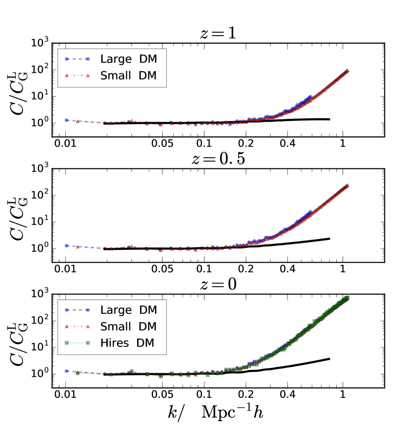
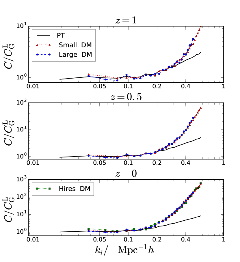
In Fig. 3, we plot the diagonal elements of for dark matter. We show the results using the three sets of simulations. The results are normalized with respect to the Gaussian covariance, in which the power spectrum is the linear one. The results from the Small and Large set agree with each other well. At low the results from the Small and Hires are very similar, thus the mass resolution effects are small at low , consistent with that reported in Ref. Blot et al. (2015). We also plot the perturbation theory results, which include the nonlinear power spectrum correction to the Gaussian covariance and the trispectrum Eq. II.1.1. The agreement between perturbation theory and simulation results seems to be worse than what shown in Ref. Takahashi et al. (2011). A possible reason is that we have used the nonlinear power spectrum from simulations, which is lower than the 1-loop one in the nonlinear regime.
We now show the correlation coefficient defined as
| (14) |
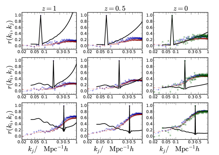
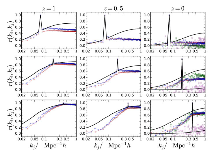
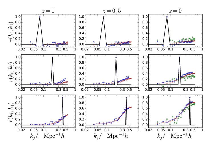
In Fig. 4 we plot as a function of , with fixed at the values of , 0.19, and respectively. is expected to be independent of the simulation volume, and indeed we find that the results from a different simulation set agree with each other well. When both and are small, the agreement between the tree-level perturbation theory and the numerical results is reasonable, but it deteriorates for large or as the mode coupling becomes more significant in the nonlinear regime. See Refs. Bertolini et al. (2016); Mohammed et al. (2016) for the improvement of the agreement by including the 1-loop corrections to the trispectrum.
For Gaussian distribution, the error of the mean goes like , while the error of the covariance is , where and are the number of modes in the bin and the number of independent realizations, respectively; see e.g. Taylor et al. (2013). As the total volume of the Large set is the same as that of the Small set, we expect them to have a simiar error bar for the mean. On the other hand, from Fig. 4, the correlation coefficients for the Large set is much noisier than that of the Small set because of small number of realizations. We find that the small scale trispectrum contribution is largely insensitive to the simulation box and this is consistent with Mohammed et al. (2016) (As we mentioned, the small differences between the Large and Small set could result from the output time fluctuations). Thus to get the small-scale covariance, we can run large number of small box size simulations to beat down the noise on the covariance without worrying about the volume effects.
II.2.2 Halos
We now look at the the covariance of the halo power spectrum. We are usually interested only in the continuous halo power spectrum signal, and the Poisson shot noise is subtracted using Eq. 66. Caution must be taken for the appearing in the shot noise formulas. The mean density of halos is obtained by ensemble average, but it is usually estimated using the volume-averaged density measured in a particular simulation/survey. We will see that using the volume average number density results in a substantially smaller covariance.
We first look at the case when the ensemble averaged number density is used. This corresponds directly to the Poisson model prediction given in Appendix C.1. The ensemble averaged number density is obtained by further averaging the volume-averaged ones over the realizations of the simulations. It is clear that in this case the covariance of the power spectrum with the Poisson shot noise subtracted is the same as that of the raw power spectrum. Here we use raw power spectrum to refer to the one measured directly from simulation without any shot noise subtraction.
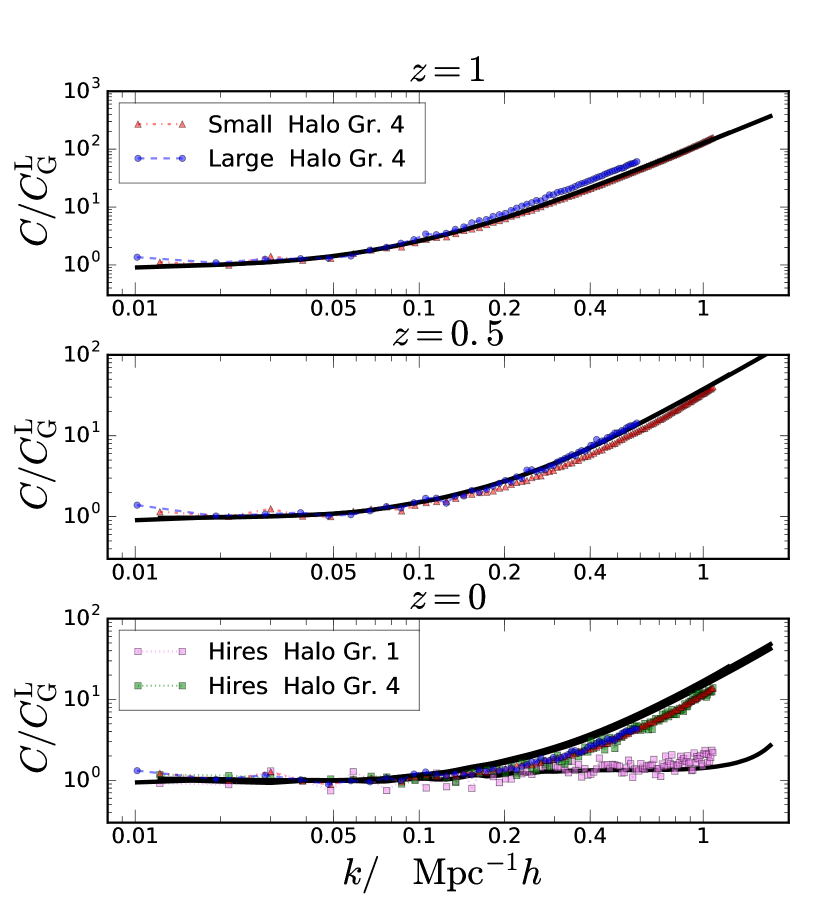
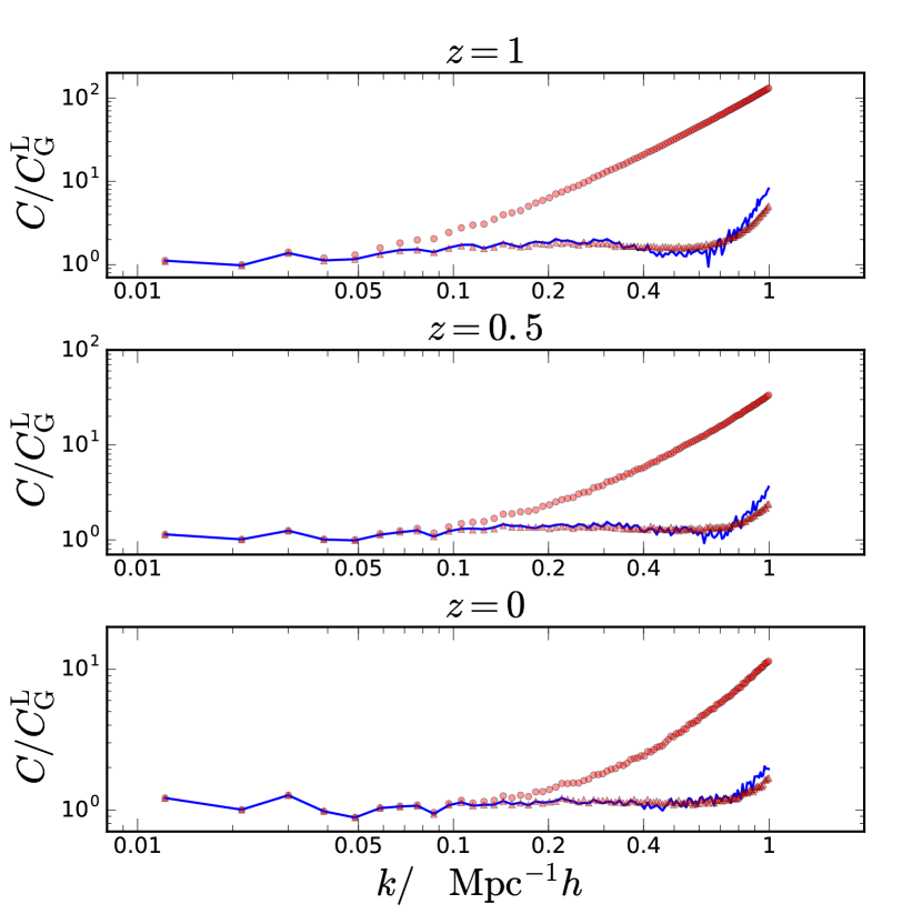
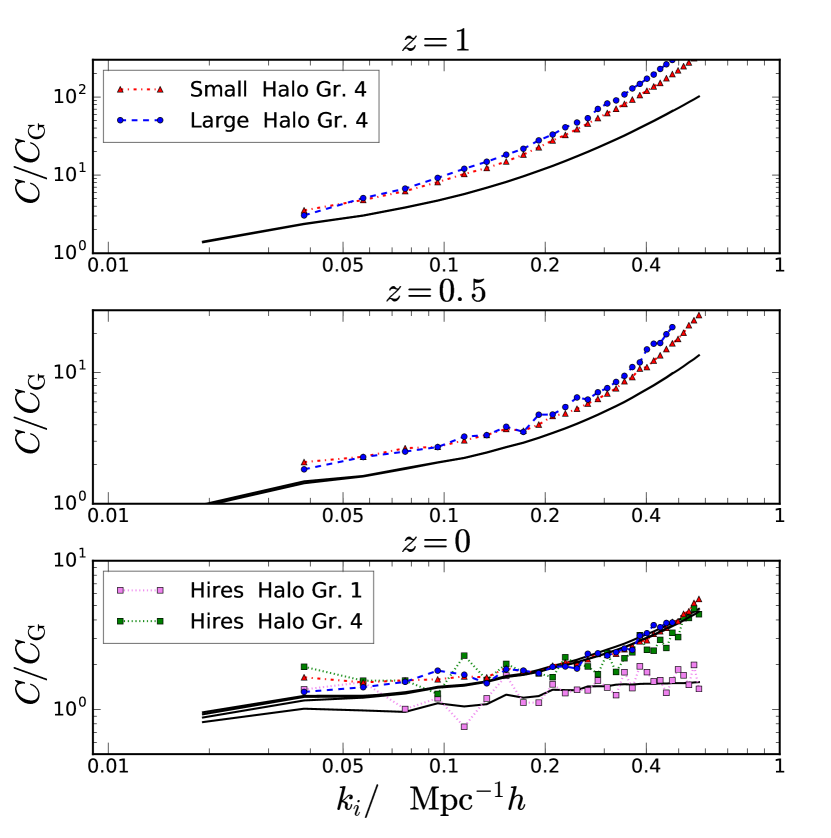
In Fig. 5, we show the diagonal elements of the covariance of the halo power spectrum. We normalize the results using the Gaussian covariance in Eq. 11. Halo groups from Large, Small, and Hires sets are used. Similar to the dark matter case, we find that the results from different sets are similar. The differences between the Large and Small may be due to the output time fluctuations. Because of the low number of realizations available, the trends for the low bias groups from the Hires set are noisy. For clarity, we only show the results from Hires group 1 and 4. Thanks to the smallness of the non-Gaussian corrections for the abundant halo group as expected from Fig. 2, the model agrees well with simulation for Group 1. Overall, the Poisson model including the non-Gaussian corrections gives a reasonably good agreement with the numerical covariance up to .
To compute the prediction we use a simple linear bias model
| (15) |
The linear bias is obtained by fitting the model to the mean of the auto power spectrum up to . The best-fit values are shown in Table 2. To compute the prediction in the Poisson model we should use the fully nonlinear polyspectra, but for the high mass group 4, we find that the results are similar even if we use the nonlinear power spectrum measured from simulations instead. However, for group 1, the nonlinear power spectrum must be used because the magnitude of the halo power spectrum is comparable to the Poisson shot noise for this abundant group.
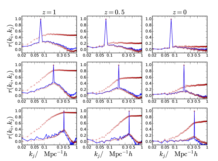
In Fig. 6, we plot the correlation coefficient for the halo power spectrum. We choose the same sets of as in Fig. 4. We note that for dark matter, generally increases as goes beyond the pivot scale , while for halos, tends to level off or increases very mildly beyond the pivot scale. When is small, the model can predict near the pivot scale, but tends to overpredict it when the separation from the pivot is large. We also note that the model performs worse at low than at high . This is because at low higher order correlators are more important.
We now consider the case when the Poisson shot noise obtained with the volume average number density is subtracted from each realization. The covariance can then be expressed as
| (16) | |||||
where is defined as
| (17) |
with being the volume-averaged number density obtained in a particular realization. In Eq. 16, we have assumed that
| (18) |
We shall see that this is indeed a good approximation. We find that the fluctuations of the number density of the halo groups in the simulation volume can be modelled as a Poisson fluctuation.
In Fig. 7 we plot the diagonal elements of the halo power spectrum covariance when the Poisson shot noise from the individual realization is subtracted. For clarity we only show the results from the Small set. Note that we still normalize the covariance using Eq. 11. First, we find that the resultant covariance becomes much closer to the Gaussian one. This is good news because for the more realistic scenario, where the mean density is computed as a volume average over the survey/simulation, the halo power spectrum covariance is reduced and is easier to predict. This makes sense intuitively since when the number density is estimated from the realization, part of the fluctuations is absorbed in the shot noise term. The distinction between the local volume-averaged density and the global ensemble one is analogous to the effects arising from defining the density contrast with the local or global average density found in Ref. de Putter et al. (2012). We show the results obtained using Eq. 16, in which the variance of the number density is measured from simulations. We see that it agrees with simulation results very well. This validates Eq. 18 and shows that the Poisson shot noise does not correlate with the clustering.
Similarly, when the Poisson shot noise is subtracted from the individual realizations correlation coefficients are also significantly reduced as shown in Fig. 8. The predictions using Eq. 18 also result in very good agreement with the simulation results. However, even though from Fig. 7, it appears that after subtraction of the individual shot noise, the diagonal elements are very close to the Gaussian one, it is clear from Fig. 8 that after subtracting the variance of , there are still large cross correlation coefficients.
In summary, our results show that the difference between the two different ways to subtract the Poisson shot noise simply arises from the fluctuation in the number density of the sample, and its effect can be modelled by a fluctuating . The fluctuations in the Poisson shot noise account for large amount of non-Gaussianity in the covariance matrix.
In the plots of this section the covariances are always normalized with respect to the Gaussian covariance. Here we comment on the magnitudes of the matter and halo power spectrum covariances. For the massive halos in group 4, the power spectrum covariance is 3 to 5 order of magnitudes higher than the matter one, depending on the redshift in question. Thus for these kinds of halos, the shot noise contribution to the covariance completely dwarfs the matter power spectrum covariance. However, as the number density of halos increases, the shot noise contribution to the power spectrum decreases. For the Hires group 2, we still find that the halo power spectrum covariance is one order of magnitude higher than that of the dark matter. When the number density is as high as that of the Hires group 1, we find that the halo covariance is comparable in magnitude to that of the dark matter. These explain why the simple linear bias model works well except for the most abundant groups. In Euclid, the number density of galaxies is expected to reach Laureijs et al. (2011), hence the covariance is expected to get non-negligible contributions from dark matter nonlinearity and galaxy biasing.
Finally we point out that Smith (2009) also studied the covariance of halo power spectrum using -body simulations although using only 30 simulations of box size . Our results are similar to those in Smith (2009) regarding the effects of different shot noise subtraction procedures to the covariance. Here we go on to show that the fluctuating Poisson shot noise term accounts for most of the non-Gaussianity.
III Covariance of the bispectrum
In this section, we first discuss the theory of the bispectrum covariance for dark matter and halo. Then we present the numerical covariance results and the comparison with theory.
III.1 Theory of the bispectrum covariance
The theoretical discussion on the bispectrum covariance in previous works has been mainly limited to the Gaussian contribution to the covariance Scoccimarro et al. (1998, 2004). This is partly because the bispectrum covariance has a relatively large number of elements and the number of available realizations in most of the existing simulation sets is not large enough to get good signal to noise. Here we will consider the non-Gaussian contribution as well. We will see shortly that this is crucial to get good agreement with the simulation results.
Given the definition of the bispectrum
| (19) |
we can construct an estimator as Scoccimarro et al. (1998, 2004)
| (20) | |||||
where indicates the integration is over a spherical shell of width , with being the width of the bin in Fourier space. The term counts the number of modes satisfying the triangle constraint:
| (21) |
In fact, we can compute analytically to get Scoccimarro et al. (2004)
| (22) |
where is defined as
| (23) |
and is given by
| (24) |
For more details on the derivation of Eq. 22, see Appendix B. In Appendix A, we check the probability distribution of . We find that it is close to Gaussianly distributed but with non-negligible skewness and kurtosis as well.
The covariance matrix of , is defined as:
| (25) | |||||
In the following we will skip the superscript in the notation for the sake of simplicity.
III.1.1 Dark matter
When is Gaussian, is zero, however does not vanish. The Gaussian covariance can be written as Scoccimarro et al. (2004)
| (26) |
where is non-vanishing only if the shape of the triangle is the same as that of . If none of the sides of the triangle are equal to each other, . If the triangles are isosceles, . For equilateral triangles, we have . The derivation of Eq. 26 is reviewed in Appendix B. In Eq. 26, for Gaussian , is the linear power spectrum. As we consider the non-Gaussian contribution below, we find that part of the contribution can be resummed if we use the 1-loop matter power spectrum instead of the linear one for one of the power spectra. However, the 1-loop power spectrum overestimates the matter power spectrum from simulation in the weakly nonlinear regime already. Similar to the case of power spectrum, we shall use the nonlinear power spectrum measured from simulations in place of the 1-loop results. We will use the notation to distinguish the case when the nonlinear power spectrum is used, that is
| (27) | |||||
where cyc. denotes cyclic permutations and denotes the nonlinear power spectrum.
In the top-left corner of Fig. 9, we show a diagrammatic representation of . The rules are the same as those in Fig. 1. The black dots on the left and right hand side represent the three ’s in each of the bispectrum estimator . The curly line represents the linear power spectrum. We put a filled circle on one of the curly line to indicate that the nonlinear power spectrum is used instead of the linear one. We see that the Gaussian term has the same structure as the Gaussian covariance for power spectrum in Fig. 1. The Gaussian covariance for the bispectrum is also inversely proportional to the number of modes in the bins (and it scales with bin width as ).
Nonlinear evolution causes mode coupling and departure from Gaussianity. At the tree-level order, there are both connected and disconnected contributions to the 6-point function. In this paper we shall evaluate the leading disconnected tree-level contributions only. We will estimate the leading connected contributions and show that they are subleading relative to the terms we consider.
The disconnected non-Gaussian tree level contributions can arise either from the or kernel. In Fig. 9, we show a graphical representation of these non-Gaussian contributions. There is one contribution due to , , in which is represented as three legs branching from a black dot. The non-Gaussian tree level can also arise from two kernels. We further classify these diagrams into type I if both kernels are on the same triangle, and type II if they are distributed on different triangles. There are two type I diagrams and four type II.
First for convenience we define the notation
| (28) |
The contribution due to reads
| (29) |
By inspecting the diagrammatic representation of in Fig. 9, it is easy to see that there are 3! permutations for and 3 permutations for as two of the legs are symmetric. There are also additional contributions from interchanging and . Thus there are altogether 36 permutations. For other diagrams the number of permutations can be worked out in a similar manner.
The type I contributions due to are
| (30) | |||||
| (31) | |||||
The type II contribution reads
| (32) | |||||
| (33) | |||||
| (34) | |||||
| (35) |
Note that the expressions are tree-level only, thus there is no loop integration, and the high-dimensional integrals result from the bin width integration. The leading non-Gaussian terms we consider here are all of the order . All the terms contain a factor of Dirac delta function , and this implies that these terms couple only triangles with at least one side equal to each other.
In each of the non-Gaussian terms there are four Dirac delta functions: two due to the triangle constraints and , and another two imposed on two disjoint sets of , , , , , and . These can also be seen by inspecting the non-Gaussian diagrams in Fig. 9. Hence it is clear that one of these latter two Dirac delta functions is redundant, and it gives . That is why in there is a factor of only. Hence the non-Gaussian terms have the same volume dependence as the Gaussian one, and we will use this observation to compare simulation results from different boxes. The other Dirac delta function relates two vectors, each coming from one of the bispectrum estimator, which is in Eq. 29–35. This Dirac delta function is analytically integrable, and thus these integrals are non-vanishing only for triangles with at least one side equal to each other. We will make use of the pattern of the Dirac delta functions discussed here to construct an efficient Monte Carlo integration method.
Except for the Dirac delta , the other two remaining Dirac delta functions in general cannot be integrated analytically. Thus the resultant 15-dimensional integral is hard to compute. High dimensionality causes problems for numerical integrators in general. The presence of the remaining two Dirac delta functions makes the integrand non-vanishing only in narrow regions. Although high dimensional integrals can often be attacked by Monte Carlo integration method, generic Monte Carlo integration would fail as they would miss the narrow peaks in the high dimensional space.
Here we present a Monte Carlo method that can efficiently sample the points that satisfy the Dirac delta function constraints. We first note that the vectors that fulfil the triangle constraint must be some small perturbations of the triangle and . Thus instead of sampling all the points in the full integration domain, we can proceed as follows. We first generate a vector in the shell randomly. For we must have . To determine the allowed variation of , we consider
| (36) |
Hence we sample uniformly in the range . To further fix , we sample the polar angle of , , uniformly in the interval . The azimuthal angle of , is fixed by the relation
| (37) |
where and are the spherical coordinates of . If the length falls within the interval , the vector is assigned to be , and the three vectors , , and are accepted, otherwise the procedure is repeated until the proposed vectors are accepted. We find that the acceptance rate can reach about 20% and it does not vary much with the triangle configuration considered. For the triads , , and , we make use of the Dirac delta function and assign accordingly. The construction of and is then similar to those for and .
After developing an efficient algorithm to sample the vectors satisfying the constraints imposed by the three Dirac delta functions, we can attack the non-Gaussian integrals using the Monte Carlo method (see e.g. Press et al. (2007) for a review). The integrals can be schematically written as
| (38) | |||||
where the integrand is averaged over the points in the integration domain defined by the Dirac delta functions. The success of this method relies on the fact that the integration volume can be computed analytically and it reads
| (39) |
where is given by
| (40) | |||||
In the Appendix B, we show the derivation of .
From Eq. 38 and 39, we find that the non-Gaussian integral corrections scale with the bin width as . In contrast the Gaussian term exhibits a stronger scaling . From Eq. 39 and 40, we explicitly see that the non-Gaussian terms scale with the volume of the simulation as , the same as the Gaussian term. The volume dependence is the same as that for the power spectrum covariance. As we mentioned, this is a consequence of the statistical translational invariance.
Ref. Kayo et al. (2013) computed the non-Gaussian contributions to the weak lensing bispectrum covariance. The structures of the terms are similar to the ones we consider here, with the main difference that their results are for 2D field, while ours are 3D. The authors classified the non-Gaussian terms into groups of order bispectrum squared, , a product of power spectrum and trispectrum, , and connected 6-point function. Our terms , , , would be classified as the order . This can be easily seen from Fig. 9 as there is a curvy line, which represents a power spectrum, directly connecting the two sides of the bispectrum estimators on the top of each of these diagrams. The rest of the diagram has the same structure as the trispectrum terms shown in Fig. 1 except . The trispectrum part in is in fact the contribution to the beat coupling for the power spectrum discovered in Hamilton et al. (2006). For the periodic boundary condition simulation we consider here, it does not contribute to the power spectrum covariance. However, it can exist in part of another diagram. The remaining terms , , and belong to the group . This is because each of the diagrams in this set can be decomposed into two bispectrum parts with each part consisting of two points from one of the estimators and another one from the other estimator.
In addition, Kayo et al. (2013) also estimated the connected 6-point function using 1-halo term in the halo model. The leading tree-level connected 6-point function is of the order of . Relative to those in Eq. 29–35, there is no explicit Dirac delta function such as in the connected 6-point contributions, thus they couple triangles of different shapes. Furthermore they do not depend on the bin width. We can make a simple estimate by taking the equilateral triangle shape and assuming kernels are of order 1. Neglecting the symmetry factors, the connected 6-point function contribution from perturbation theory is . The magnitude of the terms in Eq. 29–35 is . Thus the 6-point contribution is subdominant. For example at and , it is 7% of the non-Gaussian terms we considered here. Of course, for triangles of different shapes, the non-Gaussian terms we consider vanish, the connected 6-point contribution must be included.
Classifying the terms into groups (the Gaussian one), , , and the connected 6-point contributions provides a way to resum the perturbation series. As we mentioned, using the nonlinear power spectrum in the Gaussian term we effectively resum part of the higher order contributions. Similarly, we can replace , and with the nonlinear ones obtained either from simulation measurements or other analytic methods, such as halo model. This approach was taken in Kayo et al. (2013), but we will not pursue this further in this paper.
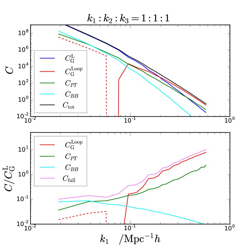
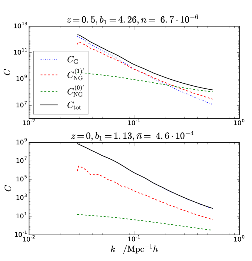
In Fig. 10, we show the contribution to the covariance for the equilateral shape. We have compared the linear Gaussian term with the high order correction to the Gaussian term and the non-Gaussian terms, which we have grouped into and respectively. We see that for , the term is the dominant non-Gaussian term, but it is negligible for high . The contribution becomes the dominant non-Gaussian contribution for . Yet still the term is small compared to the loop contribution to the Gaussian for . For the isosceles shape, the results are qualitatively similar.
III.1.2 Halos
The discrete nature of halos causes stochastic fluctuations. Similar to the case of power spectrum, the shot noise is the main source of halo bispectrum covariance as we will discuss in next section. In Appendix C.2, we use the Poisson model to derive the contribution to the bispectrum covariance due to Poisson fluctuations. In the Poisson model we assume that the point particles Poisson sample the underlying continuous density field. Both the contact correlation function due to Poisson sampling and the intrinsic correlation of the continuous field contribute to the 6-point function. This results in both connected and disconnected contributions to the 6-point function (see Eq. C.2), which are represented diagrammatically in Fig. 25. We can classify the terms (or diagrams) using the correlator expansion mentioned in Sec. III.1.1. The diagrams that are disconnected with three separate components are the Gaussian terms, and there are altogether three such diagrams. I.e. they are in the group. The diagrams with two disconnected components are either in the non-Gaussian group or . The connected diagrams represent the connected 6-point function contributions. Furthermore, within each group, there are terms with various power of , we can regard it as an expansion in . We refer the readers to the Appendix for the details. Here we summarize the main results.
There are three terms in the Poisson model that couple only triangles of the same shape, as the Gaussian term in Eq. 26. These terms contain two Dirac delta functions in the 6-point function Eq. C.2 (or three disconnected components in Fig. 25). They can be combined with Eq. 26 as
| (41) | |||||
Eq. 41 agrees with Scoccimarro et al. (1998). Although the Poisson contributions do not arise from Gaussian fluctuations, they are on the same footing as the smooth Gaussian term, we call them Gaussian terms as well.
There are also non-Gaussian contributions due to Poisson fluctuations. The non-Gaussian terms with one Dirac delta function in Eq. C.2 (with two disconnected pieces in Fig. 25) belong to the or group. As they contain the continuous correlator up to the halo tripsectrum, in this paper we shall only explicitly evaluate the terms with halo power spectrum or some terms with bispectrum. The terms with one Dirac delta function that we evaluate, denoted by here, are the ones up to the seventh line in Eq. 86. The non-Gaussian terms due to the connected 6-point function are the ones without any Dirac delta Eq. C.2 (diagrammatically, they are the connected diagrams in Fig. 25). We only explicitly evaluate the first line of Eq. 87. We will denote this by .
We plot the shot noise contributions to the covariance of the halo bispectrum in Fig. 11 for two selected halo groups, which correspond to Gr. 4 of the Large/Small simulation set at and Gr. 2 of the Hires set at . We plot the diagonal elements for the equilateral triangle configuration. The Gaussian covariance (Eq. 41) is compared with the non-Gaussian contributions and . For the low density sample, is comparable to the Gaussian one, while is sub-dominant until . For the more abundant sample, the Gaussian covariance is the dominant one comparable to the non-Gaussian contributions. Thus when the number density is high , Gaussian covariance is a good approximation. Recall that for the same sample, Gaussian covariance is also a good approximation for the power spectrum.
III.2 Numerical results
III.2.1 Dark matter
We first look into the covariance of the dark matter bispectrum. The covariance is estimated from the available realizations as
| (42) | |||||
where is the number of realizations used and is the mean of the bispectrum measured from the simulations.
We show the diagonal elements of the bispectrum covariance matrix for the equilateral triangle configuration in Fig. 12. The results are normalized with respect to the Gaussian covariance , Eq. 26. As we noted before, for both the Gaussian and non-Gaussian covariance, the volume of the simulation factors out. Thus by dividing by the Gaussian covariance, we are able to compare the simulation results obtained from different box sizes. The results from the Large, Small, and Hires simulation sets agree with each other well. We find that the non-Gaussian contribution to the covariance increases rapidly as decreases from 1 to 0 in the mildly nonlinear regime . The covariance is within 20% from up to at and at . We also plotted the non-Gaussian prediction described in Sec. III.1.1. The non-Gaussian correction gives the predictions agreeing with the simulation results up to at and at .
Similar to the case of the power spectrum, the cross-correlation coefficient is defined as
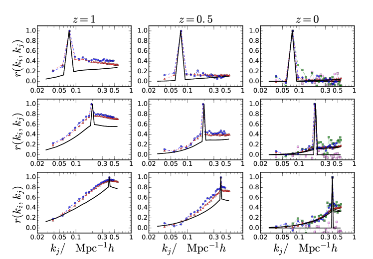
We plot for the equilateral triangle configuration in Fig. 13. In each subplot, we fix one of the lengths of the triangle and vary the length of the other one, . In these plots, we have fixed to be , , and respectively.
As we noted previously, the Gaussian covariance couples only the triangle of the same shape, while the leading non-Gaussian corrections couple triangles with at least one side equal to each other. Thus both the Gaussian and disconnected non-Gaussian tree-level corrections cannot give rise to cross correlations between equilateral triangles of different sizes. We see that indeed when both and are small, the correlation coefficients are consistent with being zero. As one of the wavenumbers increases also starts to increase. The larger the value of the wavenumbers the larger the covariance. This is expected from the fact that nonlinearity increases the coupling of different wave modes. The accuracy of the perturbation theory prediction is qualitatively similar to that for the power spectrum covariance shown in Fig. 4.
III.2.2 Halos
We now move to the halo bispectrum covariance. The Poisson shot noise contribution is given by Eq. 70, i.e.
| (44) |
where is the smooth halo power spectrum. As we are interested only in the smooth correlation function signal, the contribution to the halo bispectrum due to Poisson fluctuations is usually subtracted. Similar to the case of the power spectrum, we distinguish between the mean Poisson shot noise subtraction and the Poisson shot noise estimated and subtracted from each realization.
We first show the results when the mean Poisson shot noise is subtracted. This case corresponds precisely to the derivation done in Appendix C.2 and briefly summarized in Sec. III.1.2. In Fig. 14, we plot the diagonal elements of the covariance for the equilateral triangle configuration. The results are normalized with respect to the Gaussian covariance Eq. 41. We have also plotted the theory prediction, which includes the Gaussian term and the non-Gaussian corrections and . We find that the deviation of the numerical results from the Gaussian covariance is significant even at low for the rare mass groups Large/Small Gr. 4 at and 1. The model tends to underestimate the covariance in comparison with the numerical results. The reason is that we have only evaluated parts of the 6-point function contributions in the Poisson model. On the other hand, for the relatively more abundant groups, the deviation from the Gaussian result is mild and the model agrees with the data well. This is mainly because for these low bias groups the non-Gaussian corrections are small as we have seen in Sec. III.1.2. Note that for group 1, we have to use the measured nonlinear power spectrum to compute the Gaussian covariance as Eq. 15 is not adequate.
In Fig. 15, we plot the correlation coefficient for the halo bispectrum with the mean Poisson shot noise subtracted. The triangle configurations are equilateral. One of the wavenumbers, is fixed to be , , and respectively. The theory predictions are also overplotted for comparison. As couples triangles with at least one side equal to each other, it vanishes for equilateral triangles of different shapes. Hence only contributes to the correlation coefficient. Similar to the diagonal case, for the rare halo groups at and the model underestimates the covariance compared to the simulation results, while the model agrees reasonably well with the data for the more abundant groups at .
We now consider the scenario when the Poisson shot noise is subtracted from individual realizations. The covariance of these two scenarios is related by
| (45) | |||||
In the last line we assume that
| (46) |
We will shortly check how good this ansatz is.
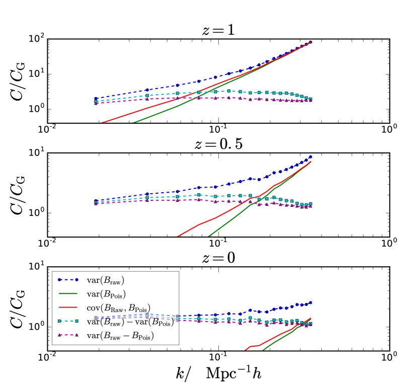
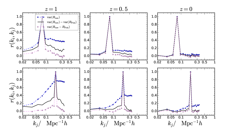
Unlike the former case, which is equivalent to no shot noise subtraction at all, we have to rely on the accuracy of the Poisson model here. We find that the shot noise subtracted equilateral bispectrum goes negative for at . At , for Gr. 4, this occurs at . Although there seems to be no fundamental reason that the smooth halo bispectrum must be positive, this may well indicate that the Poisson model is not accurate enough. Therefore we shall not show the results for beyond . In Fig. 16, we compare the diagonal elements of the covariance obtained with the mean Poisson shot noise subtraction and the individual shot noise subtraction. We normalize the covariance by the Gaussian covariance Eq. 41. Similar to the power spectrum case, the subtraction of shot noise from the individual realizations significantly reduces the covariance, and it gets much closer to the Gaussian one. From Fig. 17, we find that the off-diagonal elements also exhibit substantially lower level of correlation, especially for the groups at and 0.5. The correlations are roughly consistent with zero for the groups at and 0 within the scatter.
In Fig. 16 we also show the covariance and . At low , they are quite different, but they approach each other at high . Because we found that the number density fluctuation does not correlate with the continuous clustering, i.e. halo power spectrum in Sec. II.2.2, the difference between them must come from the continuous power spectrum in . On the other hand, at high the number density fluctuation dominates, so these two covariances agree. To test the ansatz in Eq. 45, we plot the prediction using in Fig. 16 and 17, which yields a covariance close to the one obtained by subtracting shot noise from individual realizations. This demonstrates that Eq. 46 is a reasonable approximation. Our results show that most of the non-Gaussianity in the halo bispectrum covariance arises from the fluctuations in .
We now comment on the magnitudes of the dark matter and halo bispectrum covariances. For the rare group Gr. 4, depending on the redshift, the covariance of the halo bispectrum is nine to five orders of magnitude larger than that of the dark matter bispectrum covariance. The differences decrease when the number density of the sample increases. Even for the abundant group, Hires Gr. 2, the covariance of the halo bispectrum is still an order of magnitude higher than that of the dark matter. When the number density reaches as high as that of the Hires Gr. 1 [], the magnitude of the halo covariance is comparable to that of the dark matter. Hence the relative differences are quite similar to the power spectrum covariance. This suggests that shot noise is the dominant contribution to the halo bispectrum covariance.
Gaussian covariance for the bispectrum is often used in forecast e.g. Xu et al. (2015); Welling et al. (2016); Xu et al. (2016). When the mean number density is used, our results show that the Poisson fluctuation gives rise to large non-Gaussianity in the covariance unless the number density of the sample is sufficiently high . Fortunately, in reality, the number density is estimated from the local average and by subtracting the shot noise from individual realizations, the covariance gets much closer to the Gaussian covariance. This is because most of the non-Gaussianity is due to the fluctuations in the Poisson shot noise . However, there is still significant amount of non-Gaussianity left. We will see in in Sec. IV that use of the Gaussian covariance severely overestimates the signal-to-noise ratio.
IV The information content of the power spectrum and bispectrum
As the power spectrum has been well explored, and the bispectrum becomes the next frontier in large scale structure, it is crucial to address how much information one can gain by going to higher order correlators. The signal-to-noise ratio, S/N, is often used to quantify the information content in the power spectrum and bispectrum, e.g. Takahashi et al. (2011); Scoccimarro et al. (2004); Sefusatti and Scoccimarro (2005); Blot et al. (2015). The Fisher information Tegmark et al. (1997) is an alternative way to characterize the information content. However, we shall not consider it here as it involves the derivatives of the polyspectra with respect to the cosmological parameters, which would require a dedicated set of simulations with varying cosmological parameters.
The Gaussian covariance is usually used to make forecast and quantify the information content. In particular, the forecast based on the Gaussian covariance suggests that there is a lot of information in the bispectrum (Sefusatti and Scoccimarro (2005), see also below). However, since we have seen in the previous sections that the non-Gaussian contributions significantly increase the covariance already in the weakly nonlinear regime, it is important to ask how the results are modified when the non-Gaussian covariance is taken into account.
The signal-to-noise ratio is defined as
| (47) |
where is the inverse of the covariance matrix, also called the precision matrix, and is the signal. Here we use the non-Gaussian covariance measured from simulations to quantify the information content in the power spectrum and bispectrum. For dark matter, the signal is simply the mean of the measured power spectrum and bispectrum respectively. For halos, we use the power spectrum and bispectrum with the Poisson shot noise subtracted, using Eq. 66 and 70 respectively, with the Poisson shot noise estimated and subtracted from each realization. At high the Poisson shot noise subtracted power spectrum and bispectrum can go negative, which is deemed unphysical, hence we shall only show the results that are reliable. We also show the results obtained using the Gaussian covariance for comparison.
There is one more complication because we require the precision matrix rather than the covariance matrix. Ref. Hartlap et al. (2007) pointed out that for a covariance matrix, must be smaller than the number of realizations, , for the covariance matrix estimated from the realizations to be invertible. The basic reason is that we can regard each realization as an independent random vector in -dimensional space. When is larger than , these vectors are sufficient to span the space of dimension , otherwise the rank of the covariance matrix is less than . See Hartlap et al. (2007); Anderson (2003) for a formal proof. Moreover, even when the covariance matrix is invertible, because inversion is a nonlinear operation, the inverse of an unbiased estimator is in general biased. If the distribution of the estimator is Gaussian, the bias-corrected estimator for the precision matrix reads Hartlap et al. (2007); Anderson (2003)
| (48) |
where is the unbiased sample covariance matrix.
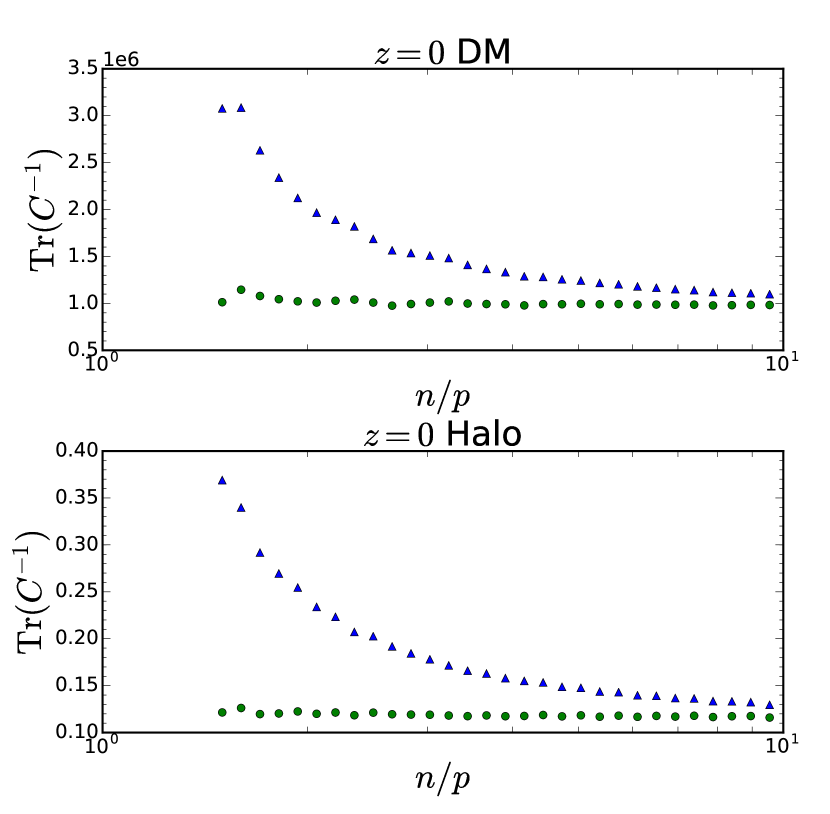
For the power spectrum the number of bins, , is typically smaller than the number of realizations available in our case, e.g. the maximum number of bins for the power spectrum is 90. Ref. Blot et al. (2016) checked that Eq. 48 works very well for the power spectrum precision matrix when . On the other hand, because of the large number of configurations, the number of bins of the measured bispectrum can be comparable to or even larger than the number of realizations that we use. For example, for the binning of the Small simulation set that we used in the previous sections, there are 2825 bins.222 We can compute the total number of distinct triangle configurations (including the folded ones) with the formula , where and are the ceiling and floor functions. This formula is derived from the integer sequence A002620 in https://oeis.org/A002620 (see also Jenkyns and Muller (2000)). In this case we use bins, and we get 2825 configurations. As Eq. 48 assumes that the distribution of the bispectrum estimator is Gaussian, a priori it is not clear how well it works for the bispectrum covariance. In Appendix A, we check that the distribution of the bispectrum estimator follows the Gaussian distribution reasonably well, although there are also some non-negligible deviations. To test Eq. 48, we shall use the Small simulation set as it has the largest number of realizations. Because the key parameter in Eq. 48 is the ratio , we rebin the bispectrum into wider bins so that the sides of the bispectrum are in units of instead of that we have been using so far. After rebinning, there are altogether bins of bispectrum configurations. As the correction is only an overall factor, following Hartlap et al. (2007), we plot the trace of the precision matrix against in Fig. 18. We show the dark matter and halo data from the Small set at . Each data point in this figure corresponds to the results obtained with a precision matrix estimated by randomly choosing realizations from the total 4096 ones. We compare the results from the naive estimate and the bias-corrected estimate . As increases, the naive estimate decreases and approaches the bias-corrected estimate. For , the correction works very well already. Note that for we encounter difficulties in inverting the covariance matrix due to the reason mentioned above. As Eq. 48 works very well, we shall use the bias-corrected precision matrix for both power spectrum and bispectrum.
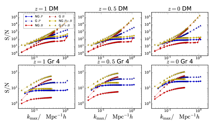
Finally, we are ready to present the S/N of the power spectrum and bispectrum. We will only show the results from the Small set due to its large number of realizations available. However, we will also comment on the results from Hires. In Fig. 19, we plot the for both dark matter and halo power spectrum against the maximum used to compute the S/N, . For the power spectrum, the S/N does not depend on the binning width used to the lowest order. Of course there is some binning dependence if the field varies appreciably across the bin, but this dependence is of higher order in the binning width. A similar statement was also made in Takahashi et al. (2011). We verify it in Appendix D.
We find that for the power spectrum of dark matter, the information content increases as increases in the linear regime. The S/N then starts to level off at the weakly nonlinear regime . The flattening of the S/N becomes more and more serious as the redshift decreases. In particular at , there is almost no increase in the S/N beyond . In contrast, the obtained with Gaussian covariance keeps on increasing with the phase volume. The saturation of the information content of the dark matter in the weakly nonlinear regime has been observed by many authors Rimes and Hamilton (2005); Neyrinck et al. (2006); Lee and Pen (2008); Takahashi et al. (2011); Blot et al. (2015). This casts doubts on the efforts to model the nonlinear power spectrum accurately beyond the BAO scales and has motivated using alternative statistics to extract information from the large scale structure, notably the log transform Coles and Jones (1991); Neyrinck et al. (2009); Carron and Neyrinck (2012). Nevertheless, Fisher analysis seems to suggest that the information content on cosmological parameters is not completely erased in the nonlinear regime Blot et al. (2016).
We find that the Poisson shot noise subtracted halo power spectrum goes negative for in between 0.5 and for Gr. 4. Because the power spectrum must be non-negative, this is mathematically inconsistent. This happens when the signal is so low that the theoretical uncertainty of the Poisson model is larger than or comparable to the signal. As we believe the contribution to the cumulative signal-to-noise from this range of data is negligible, we will show it as well. For the halo power spectrum, the trends are qualitatively similar to that of the dark matter and they are roughly constant at depending on the number density of the sample. The saturation of the information content of the halo power spectrum is also hinted in Angulo et al. (2008); Smith (2009). We find that the signal-to-noise is in between a factor of a few to one order of magnitude lower than that of the dark matter for the rare halo group Gr. 4. Reassuringly for the more abundant groups from Hires, the S/N is comparable to that of the dark matter. We find that the Gaussian approximation overestimates the S/N by a factor of two to a few at .
We now turn to the for the bispectrum. We consider all the triangle configurations with the sides of the triangle less than certain , against which is plotted in Fig. 19. In order to sample the low modes well, and also to be able to probe the S/N to high , we combine the results from two different binnings for the bispectrum measurements. For the low results we use , while for high we bin the bispectrum with . In Appendix D, we verify that the S/N is invariant to rescalings of the bin width to the lowest order.
For the dark matter bispectrum, already at the S/N increases significantly slower than what the Gaussian predictions suggest. The departure from Gaussian prediction sets in at lower and lower as the redshift decreases. We also find that the deviation generally occurs at lower than the case of the power spectrum, thus suggesting that the Gaussian approximation is worse for the bispectrum. The non-Gaussian contribution significantly degrades the S/N for the bispectrum. For example, at , according to the Gaussian covariance predictions, the S/N of the dark matter bispectrum should surpass that of the power spectrum at , while the full non-Gaussian case shows that the S/N of the bispectrum is only 30% of the power spectrum value. However, it is encouraging to find that relative to the dark matter power spectrum, whose S/N already saturates at , the S/N of the bispectrum still keeps on increasing mildly up to . Interestingly, at , the S/N increases sharply and overshoots the S/N of the power spectrum. Thus by delving into the nonlinear regime, the information gain of the bispectrum is higher than that from the power spectrum. We note that the information content of the dark matter power spectrum was found to increase sharply at beyond the plateau Rimes and Hamilton (2005); Neyrinck et al. (2006). We suspect that this sharp rise in bispectrum S/N also due to the same reason. However, we shall not investigate this further here.
After the Poisson shot noise subtraction, the halo bispectrum of Gr. 4 at starts to go negative for . For Gr. 4 at , it happens at even lower , . This occurs at lower than that for the halo power spectrum. This first happens for the triangles of shape close to the equilateral. As increases, we find that more squeezed shapes also become negative. Although there appears to be no fundamental reason that the bispectrum must be positive, we believe these negative values could well indicate that the Poisson model is not reliable as the bispectrum signal gets too small. To be conservative, we shall not show the halo bispectrum results beyond . For the halo bispectrum case, the overall trends are also similar to that of the power spectrum. Again for these rare groups shown, the Gaussian approximation significantly overestimates the S/N, even more seriously than for the dark matter bispectrum. At , the S/N can be overestimated by as much as an order of magnitude. However, the Gaussian approximation gets better for the more abundant groups, and the overestimation is narrowed to a factor of a few at .
We also show the S/N obtained by combining the power spectrum and bispectrum measurements. We have properly included the cross covariance between the power spectrum and bispectrum in the joint covariance matrix. The covariance between the power spectrum and bispectrum are in general non-negligible. We will leave it for future work to model the cross covariance in details. The joint S/N coincides with the power spectrum one in the low regime. In the mildly nonlinear regime, the total S/N is slightly higher than that of the power spectrum, this suggests that the power spectrum is the main source for the total S/N. The S/N also saturates for , similar to the trend of the power spectrum.
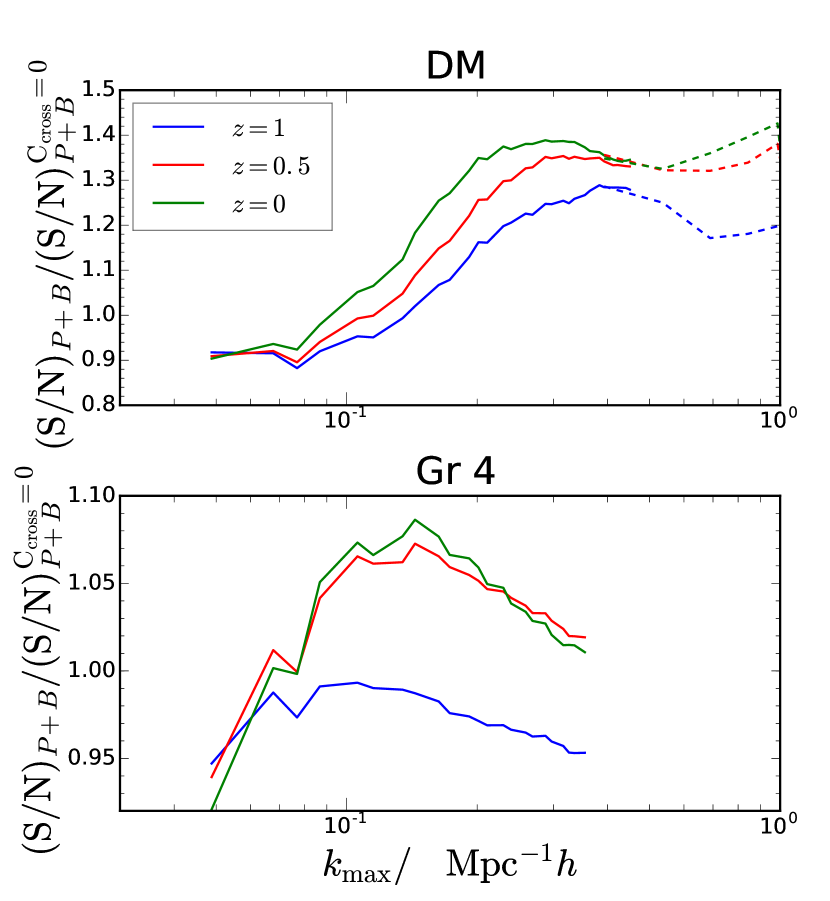
As a contrast, we compare with the case that the cross covariance between and ignored in Fig. 20. For dark matter, the cross covariance lowers the total S/N at low by 10%, while in the high regime, it is enhanced by 20 to 40%. We find that the effect of the cross covariance is smaller for the case of halos. When the shot noise is large (), the cross covariance lowers the total S/N by a few per cent up to . For higher abundance, the trend is qualitatively similar to the dark matter case, and the cross covariance enhances the S/N by a few per cent in the mildly nonlinear regime. On the other hand, the amount of S/N in the nonlinear regime is much less than that suggested by the Gaussian covariance approximation. Our results shows that adding the bispectrum information to the power spectrum only improves the total information content mildly.
In the context of weak lensing, the authors of Kayo et al. (2013) compared the S/N ratio for power spectrum and bispectrum, and the total, using the non-Gaussian covariance. Their results are consistent with ours; in particular, they also found that non-Gaussian covariance significantly degrades the S/N in the nonlinear regime.
In cosmology, we are ultimately interested in how well the measurements of the polyspectra can put constraints on the cosmological parameters, and this can be estimated using the Fisher analysis. Furthermore, it has previously been shown that the Fisher analysis results may not be easily interpreted from a simpler signal-to-noise analysis. For example, ref. Repp et al. (2015) found that the power spectrum can still place strong constraint on the parameters which are not sensitive to the amplitude of the power spectrum in the nonlinear regime (see also Blot et al. (2016)). We will leave a Fisher analysis for the combined power spectrum and bispectrum for future work (for weak lensing, see Sato and Nishimichi (2013); Kayo and Takada (2013)).
V Conclusions
Gaussian covariance is often assumed in making a forecast. In this paper, we have used a large suite of simulations from the DEUS-PUR project to study the covariance of the power spectrum and bispectrum, paying special attention to quantifying the effects of the non-Gaussian contributions to the covariance. This work is the first to use such a large number of -body simulations (altogether 4704) to estimate the covariance of the bispectrum.
We find that the non-Gaussianity is significant in the dark matter bispectrum covariance. The diagonal elements of the covariance of the dark matter bispectrum already deviate from the Gaussian covariance at by 10 % at . The correlation increases as the redshift decreases and we find that at the correlation coefficient is within 20% if and are less than for the equilateral triangle configurations. The covariance of the dark matter bispectrum significantly increases in the mildly nonlinear regime. To compare with the simulation results, we have computed the leading disconnected non-Gaussian corrections in the 6-point function. Including these non-Gaussian corrections we find that the predictions give good agreement with the simulation results in the weakly nonlinear regime. For the equilateral triangle configurations, the diagonal term agrees with the simulation results up to at and at .
We have also studied the covariance matrix of the halo power spectrum and bispectrum. We distinguished between the case when the mean Poisson shot noise is subtracted and the Poisson shot noise is estimated and subtracted from each realization. On the theory side we used the Poisson model to derive the Poisson shot noise contribution to the covariance of the power spectrum and bispectrum. The model corresponds to the scenario in which the mean Poisson shot noise is subtracted. For the power spectrum, the Poisson model describes the diagonal elements of the covariance matrix reasonably well, but it tends to overpredict the correlation coefficients. For the bispectrum, the model underpredicts the covariance, especially when the number density of the sample is low. The covariance of the power spectrum and bispectrum depend on the 4-point and 6-point functions respectively. The expansion contains large number of terms and also various high order correlators. In the prediction, we only computed the terms with the power spectrum terms and some of the bispectrum terms. This can cause part of the disagreement between the model and simulation results.
On the other hand, in simulations or observations, we often have to estimate the shot noise using the volume-averaged density. When the individual Poisson shot noise is subtracted, we find the halo covariance is significantly reduced and gets close to the Gaussian covariance. These hold for both the halo power spectrum and bispectrum. This is because most of the non-Gaussian covariance arises from the fluctuations in the Poisson shot noise term. Therefore, although the shot noise covariance is large, in reality because we use the number density estimated from the simulation/survey directly to subtract the shot noise, the halo covariance is close to the Gaussian covariance.
We note that the magnitudes of the halo power spectrum and bispectrum covariances are generally higher than those of the dark matter ones. The magnitudes of the halo power spectrum and bispectrum relative to those of the dark matter are quite similar. The shot noise contribution decreases as the number density of halos increases. Even when the number density is , the halo covariance is still higher than that of the dark matter by one order of magnitude. Thus matter nonlinearity and halo biasing are not expected to play an important role in this case. Only when the number density is as high as , the covariance of the matter polyspectrum is comparable to that of the halo.
In this work we consider simulations with periodic boundary conditions; thus the supersample covariance does not contribute. The study of the impact of the bispectrum supersample covariance will be presented elsewhere. We have compared the simulation results obtained from the Large and Small box sizes, and found that the power spectrum and bispectrum covariances are not sensitive to the volume of the box as expected from theory. Hence, to efficiently beat down the noise on the covariance, we can simulate the small scale non-Gaussianity using small box size.
As the power spectrum has been well explored, it is important to ask how much information one can gain by studying the bispectrum in large scale structure. In the second part of the paper, we have quantified the information content of the power spectrum and the bispectrum with the S/N ratio using the non-Gaussian covariance matrix measured from simulations.
The S/N of the dark matter power spectrum reaches a plateau in the mildly nonlinear regime. This is because in this regime the covariance increases faster than the signal, causing the S/N to reach a plateau. At , it flattens at . This is in line with the findings of previous works. Similarly, we find that the S/N of the halo power spectrum flattens in the regime depending on the number density of the samples. The S/N of the halo power spectrum increases as the number density of the sample increases. We find that at only the samples with number density yield the S/N comparable to that of dark matter. In contrast, the Gaussian covariance approximation overestimates the S/N by a factor of two to a few at , depending on the number density of the sample.
For the bispectrum, we have computed the S/N using all the triangle configurations with lengths less than certain . For the case of the dark matter bispectrum, the S/N increases much slower than the Gaussian approximation suggests. For example, at , the S/N at is an order of magnitude lower than the Gaussian result. Although the Gaussian covariance suggests that the S/N of the matter bispectrum surpasses that of the matter power spectrum at at , using the non-Gaussian covariance we find that the S/N is only 30% of the Gaussian one at this scale. In the nonlinear regime, the S/N of the dark matter bispectrum is still mildly increasing but it stalls at . The S/N of the halo bispectrum shares similar trends as that of the matter bispectrum. The Gaussian covariance approximation significantly overestimates the S/N. We find that the overestimation varies from an order of magnitude for the rare sample [] to a factor of a few for the abundant sample [] at for the redshift range considered.
We conclude that the bispectrum S/N is degraded more seriously by nonlinearities and shot noise relative to the power spectrum S/N. Thus the bispectrum only adds a small amount of increment to the total S/N when the bispectrum is combined with the power spectrum.
Despite more than a decade of efforts to measure the 3-point statistics in Fourier space Feldman et al. (2001); Scoccimarro et al. (2001); Verde et al. (2002); Gil-Marín et al. (2015) and configuration space Jing and Boerner (2004); Gaztañaga and Scoccimarro (2005); Wang et al. (2004); Marín (2011); Marín et al. (2013); Slepian et al. (2015); Guo et al. (2016), the information gain that we get is still modest compared to that from the 2-point statistics. It is well-known that the 3-point statistics are more sensitive to nonlinearities and halo biasing, both the local Fry and Gaztañaga (1993) and nonlocal Chan et al. (2012); Baldauf et al. (2012) ones. This is both a blessing and curse. On one hand, it is easier to estimate the nonlinear coupling and higher order bias parameters using bispectrum. On the other hand, it suffers from stronger nonlinear effects and is harder to model. In this sense our analysis simply reveals the cursing part that strong nonlinearities cause large information loss.
Given the low S/N of the bispectrum, it is not very useful to constrain the cosmological parameters alone. However, there are subtle effects for which the bispectrum analysis is particularly useful. When the power spectrum is combined with the bispectrum, some degeneracies can be broken. For example the degeneracy between the linear bias and the growth rate can be broken when the halo power spectrum is combined with the halo bispectrum. The bispectrum is also an important tool to constrain primordial non-Gaussianities. These subtle effects are not reflected in the general signal-to-noise analysis.
As we are ultimately interested in how well the polyspectra can constrain the cosmological parameters, the Fisher matrix analysis is preferable. Previous works found that the power spectrum in the nonlinear regime can still constrain some of the cosmological parameters which are not sensitive to the amplitude of the power spectrum Repp et al. (2015) and that the weak lensing bispectrum can yield strong constraints on the cosmological parameters even though its S/N is relatively low Sato and Nishimichi (2013); Kayo and Takada (2013). We leave the Fisher analysis for future work.
Even though we have only analysed the cases of the power spectrum and bispectrum, we speculate that higher point correlators, such as the trispectrum, may suffer information loss due to nonlinearities and shot noise even more seriously than the Gaussian approximation suggests. If this is true, then it is not a fruitful program to keep on measuring the correlation hierarchy. We can instead consider alternative ways to extract information. Some of the interesting methods include log transformation Coles and Jones (1991); Neyrinck et al. (2009); Carron and Neyrinck (2012), the clustering of voids Hamaus et al. (2014); Chan et al. (2014); Clampitt et al. (2016); Kitaura et al. (2016); Hamaus et al. (2016) and trying to recover information from the phases of the density field Chiang et al. (2002); Wolstenhulme et al. (2015); Eggemeier et al. (2015).
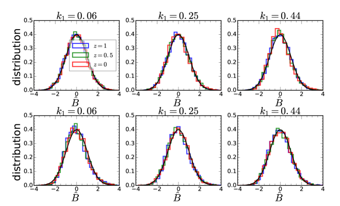
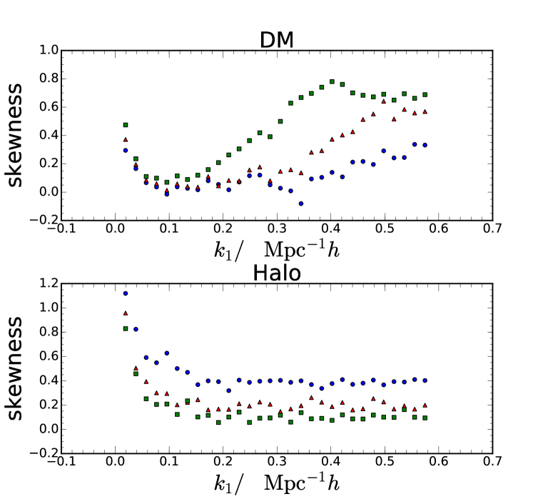
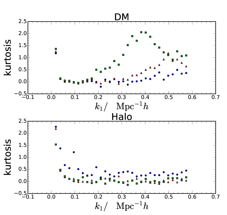
Acknowledgment
We are grateful to Martín Crocce, Azadeh Moradinezhad, Jorge Noreña, and Ravi Sheth for useful discussions, and Yann Rasera for help with the simulations. We thank Masahiro Takada and the referee for comments on the draft. We thank the members of the DEUS Consortium333http://www.deus-consortium.org for sharing the data with us. This work was granted access to HPC resources of IDRIS through allocations made by GENCI (Grand Équipement National de Calcul Intensif). K.C.C. and L.B. acknowledge the support from the Spanish Ministerio de Economia y Competitividad grant ESP2013-48274-C3-1-P.
Appendix A The distribution of the bispectrum estimator
The distribution of the estimator being Gaussian is crucial for many analytic results, e.g. the bias correction formula Eq. 48. Refs. Takahashi et al. (2011); Blot et al. (2015) checked that the power spectrum estimator for dark matter follows the Gaussian distribution well. The skewness and kurtosis of the estimator agree with the chi-square distribution, which is a consequence of the underlying density field being Gaussian. However, Blot et al. (2015) also found that the skewness deviates from the chi-square distribution result at low for . In this section, we shall check the distribution of the bispectrum estimator (Eq. 20).
In Fig. 21, we plot the distribution of the bispectrum estimator. We have transformed the measured data to the standard normal variable as
| (49) |
where and are the mean and the standard deviation of the data. Here we use the data from the Small simulation set at , 0.5 and 0, and only the results from the equilateral triangle configuration are shown. Upon comparison with the standard normal distribution, we find that the data across the three redshifts follow the Gaussian distribution reasonably well. Furthermore, the results for both dark matter and halos are similar. The tendency for the distribution to be Gaussian results from the central limit theorem because in the estimator Eq. 20, a large number of modes are averaged over. Nonetheless we note that there are some visible deviations from Gaussianity.
There are two counterinteracting effects at work. First, the central limit theorem works asymptotically for a large number of samples. When increases, there are more modes available to be averaged over in the estimator, see Eq. 22. Thus we expect the central limit theorem to perform better for high . On the other hand, the underlying density field becomes more non-Gaussian and the modes couple with each other at high . This violates the key assumption that the samples are independent in the central limit theorem. Therefore we anticipate that the central limit theorem will fail at both the low and high regimes.
In order to quantify the deviation from Gaussianity, we compute the sample skewness and kurtosis as
| (50) | |||||
| (51) |
We plot the skewness in Fig. 22. If the underlying density field is exactly Gaussian, as the skewness is essentially the 9-point function of the underlying density field, it will vanish. Thus the finite value of the skewness is an indication of the deviation of the underlying density field from Gaussianity. For dark matter, at low we find that the skewness is large precisely because the number of modes available to estimate the results are small. The skewness first decreases but eventually increases again as increases. This is because the mode coupling in the underlying density field increases in the nonlinear regime. The fact that the lower the redshift the larger the value of the skewness supports this interpretation. For the halo, we again find that the skewness is large at low . The skewness increases with redshift and this can be attributed to the fact that there are larger Poisson fluctuations at high redshift due to lower number density. On the other hand, we also find that as increases the skewness saturates to some constant value, which is harder to understand.
We present the kurtosis in Fig. 23. For the dark matter bispectrum, similar to the skewness, we find that kurtosis is large at low , and then decreases to zero as increases, but eventually increases again at high . Curiously, there is a bump in the kurtosis at at . We checked and confirmed that for other shapes, their kurtosis also exhibits a bump. This bump is hard to interpret without a concrete model. Note that there is a small bump in skewness as well, however, this is not present in other shapes. The halo bispectrum kurtosis behaves in a similar way to the skewness.
We have checked that the results are qualitatively similar for other shapes.
Appendix B A collection of derivations
In this appendix, we present the derivations of some of the formulas used in the main text.
B.1
B.2 Gaussian covariance of the bispectrum estimator
For Gaussian , the only non-vanishing contribution to the Gaussian covariance (Eq. 26) reads
| (55) |
is non-vanishing only if the shape of the triangle is the same as that of . If none of the sides are equal . If the triangles are isosceles, . For the equilateral triangle, we have . Both and arise from the fact that the three Dirac delta functions must be satisfied and the number of contractions that they can be satisfied.
Then we can simplify it further as
| (56) | |||||
where in the last line we have assumed that the bin is narrow and have taken the power spectra out of the integral. We note that in the first line, there is factor of . This arises from the structure that there are two sets of Dirac delta functions, and , and , , and . Hence one must be redundant, it results in . We find a similar pattern for the dark matter bispectrum non-Gaussian covariance terms as well.
B.3 Integration domain volume
The volume of the integration domain defined by the Dirac delta functions in the dark matter bispectrum non-Gaussian covariance terms can be computed analytically as
We can expand using the addition theorem for the spherical Bessel function (Eq. 10.1.45 in Abramowitz and Stegun (1964))
| (58) |
After taking the angular integrals of and , we get
| (59) |
Using Eq. 53, we arrive at
| (60) |
The result is the same for .
Appendix C Poisson shot noise contribution to the covariance of the halo power spectrum and bispectrum
In this section, we derive the Poisson shot noise contribution to the covariance of the halo power spectrum and bispectrum. We consider the Poisson model in which the number density of the tracers is given by
| (61) |
The discrete density contrast is defined as
| (62) |
where is the mean number density . In this section, all the smooth correlators such as , , , etc, refer to the nonlinear correlators of the tracers. The tracers can be unbiased such as the dark matter particles in -body simulations. Halos are the prototypical example of biased tracers. The Poisson model can be applied to both kinds of tracers.
C.1 Poisson shot noise contribution to the power spectrum covariance
To get the Poisson shot noise contribution to the covariance of the power spectrum we will need the Poisson shot noise contribution to the 2-point and 3-point functions as well. As the computations are similar but less cumbersome, it is instructive to first review the derivations for the 2-point and 3-point functions. One can also include weighting, see Ref.Chan and Scoccimarro (2012), however we will not consider this here. In Ref.Matarrese et al. (1997) the correlators including the Poisson shot noise are derived using an elegant functional method. Ref. Smith (2009) applied the Poisson model to compute the shot noise contribution to the covariance of the cross power spectrum between matter and halo. We will compare our results with theirs whenever possible.
The 2-point correlation of the discrete field is given by
| (63) |
The 2-point correlator of can be written as
| (64) | |||||
In this section, all the dummy indices in the summation are unequal. For discrete points, we need to separate the part when two points are the same from the case when the points are different. The latter case can be modelled by the smooth correlation function . Therefore the discrete correlation function can be written as
| (65) |
Upon Fourier transforming, the discrete power spectrum reads Peebles (1980):
| (66) |
where is the continuous power spectrum and . This is the well-known shot noise correction for the power spectrum (the presence of is due to the Fourier convention used in this paper).
Similarly the discrete 3-point function reads
| (67) |
where cyc. denotes cyclic permutations. As in Eq. 64, we can express the 3-point correlator of as
| (68) | |||||
where is the continuous 3-point function. For convenience, we have used to denote , etc.
| (69) |
In Fourier space we get the discrete bispectrum Matarrese et al. (1997)
| (70) |
with being the continuous bispectrum.
The discrete 4-point correlation function is given by
| (71) | |||||
The 4-point function of reads
| (72) | |||||
where is the continuous 4-point function.
In Fourier space, the 4-point correlator
| (74) | |||||
where is the continuous 4-point correlator in Fourier space. Note that is not the trispectrum as it usually refers to the connected part of the 4-point function only, while contains the disconnected part as well. Ref. Matarrese et al. (1997) wrote down the connected trispectrum, which corresponds to the terms without in Eq. 74.
Recall that the covariance of the power spectrum is given by
| (75) |
The covariance operator in Eq. 75 is now given by
| (76) | |||||
The first line of the RHS of Eq. 76 are the Gaussian terms. Although we use the terminology “Gaussian” here, these terms are not related to the Gaussian distribution. In fact in the Poisson model, the discrete particles are Poisson distributed. They are called Gaussian because they contribute only to the diagonal covariance as the smooth Gaussian terms. The second and third lines are the non-Gaussian terms and they can couple different bins. The last line is the continuous part of the 4-point function.
We can easily integrate over the Gaussian terms in the first line to get
| (77) |
This term can be combined with the Gaussian contribution from the continuous part as
| (78) |
Eq. 78 agrees with Ref.Feldman et al. (1994). In other words, the Gaussian covariance of the power spectrum for the halo is the same as the case for dark matter except with the dark matter power spectrum replaced by the halo one plus the shot noise term.
The non-Gaussian contribution due to the Poisson shot noise is given by
| (79) | |||||
Ref. Smith (2009) also derived the shot noise contribution to the power spectrum covariance. Comparing Eq. 79 to the result in Ref. Smith (2009), besides the minor difference that we have assumed small binning width to simplify the expressions, we note that the terms are missing in Smith (2009). These terms do not vanish in general. Suppose the tree level halo bispectrum is used for , although the local -term and the nonlocal bias term Chan et al. (2012) both vanish because they are generated by large-scale gravitational evolution, the local nonlinear bias term gives finite contribution .
C.2 Poisson shot noise contribution to the bispectrum covariance
The complexity of the perturbation series increases rapidly when the number of points in the -point function increases. We will first summarize a set of diagrammatic rules to represent the -point correlation function for , 3, and 4. Apart from the Dirac delta function, the rules are similar to the continuous case. In real space, we can represent the Dirac delta function by a new link between the points and . This link is analogous to the continuous correlation function. We can further simplify the diagram by shrinking all the points linked by the Dirac delta functions to a dot. Graphical representations of the 2-point, 3-point, and 4-point correlation functions for Eq. 65, 69, and 73 are shown in Fig. 24. For example the first two diagrams in Fig. 24 denote the two terms in Eq. 65. The first circle-dot represents the two points connected by a ; the wavy line in the second diagram denotes the continuous correlation function . In the second line, the diagrams represent the three terms in Eq. 69. The first diagram denotes the three points connected by Dirac delta functions. In the second diagram, the circle-dot represents the two points connected by the Dirac delta function and they are connected to the third point by a correlation function. The last one represents the three points connected by the continuous 3-point function. By comparing Eq. 73 with the diagrams for the 4-point function in Fig. 24, it is clear that similar rules apply. The terms that contribute to the Gaussian covariance of the power spectrum are the two disconnected diagrams in the 4-point function. Among the non-Gaussian terms, the one as a circle-dot corresponds to , and the second and fourth diagrams in the third row of Fig. 24 represent the terms with power spectrum in the first line of Eq. 79.
We now apply the rules to the 6-point function and the results are shown in Fig. 25. They are arranged based on the number of Dirac delta functions, ranging from 5 to 0. From these diagrammatic representations, it is straightforward to write down the discrete 6-point function
| (80) |
where and are the continuous 5-point and 6-point functions. Note that some of the diagrams correspond to more than one term in Eq. C.2.
Then in Fourier space, the 6-point function reads
| (81) |
where and are the Fourier transform of the continuous 5-point, and 6-point functions. In Ref. Matarrese et al. (1997), the 6-point function including the Poisson shot noise, but limited to connected terms only, was written down. They agree with the terms without in the first three lines of Eq. C.2.
We are going to classify the terms in based on the number of Dirac delta functions. This is directly related to the correlator expansion we mentioned in Sec. III.1.1. The terms with two Dirac delta functions in Eq. C.2 (highlighted in red) are the Gaussian terms, and they are in the group. Diagrammatically, they are represented by the disconnected diagrams with three disconnected parts, i.e. the most disconnected diagrams in Fig. 25. The terms with one Dirac delta function in Eq. C.2 (highlighted in green) belong to either the or group. They are the diagrams with two disconnected parts in Fig. 25. Finally, the connected 6-point function contribution in Eq. C.2 (in plain black) is represented by the connected diagrams in Fig. 25. In each group of terms, we can regard it as an expansion in . Depending on the relative importance of and , we can retain the terms with high or low power of . As contains connected 2, 3, 4, 5, and 6-point functions in general, it is formidable to evaluate in the most general case. To proceed, in this paper, we will only explicitly evaluate the terms containing the continuous power spectrum or bispectrum.
Using the shorthand notation in Eq. 28, the shot noise contribution to the covariance can be written as
| (82) |
where is defined as
| (83) |
First the terms with two Dirac delta functions in Eq. C.2 are the Gaussian terms. They are non-vanishing only if triangle is the same as . There are altogether three such terms in , and they are highlighted in red in Eq. C.2. However, because of the triangle constraint, all the Dirac delta functions in these three terms must couple one of the vectors in with another one in to give non-vanishing contribution to the covariance. This leaves us with
| (84) |
This term can be combined with the continuous Gaussian terms . Therefore, in the presence of Poisson shot noise, Eq. 26 is modified to
| (85) |
Eq. 85 agrees with the results in Scoccimarro et al. (1998). Clearly, these terms would be classified as in the correlator expansion we mentioned in Sec. III.1.1. Again, similar to the case of power spectrum, the Gaussian covariance of the halo bispectrum including the shot noise contribution can be obtained by replacing the continuous power spectrum with the halo power spectrum plus the shot noise contribution. Similar to the comments for the Gaussian power spectrum covariance, they are called “Gaussian” here simply because they are on the same footing as the “true” Gaussian terms, not because they arise from the Gaussian distribution.
We now look at the terms with one Dirac delta function in . There are altogether 14 such terms, and they are highlighted in green in Eq. C.2. Some of them can be computed analytically making use of Eq. 40. Among these terms, there are terms with Dirac delta function connecting three vectors, . When three of the vectors are from the same bispectrum estimator, they are exactly cancelled by the corresponding terms in . The net results due to the terms with one Dirac delta function in are
| (86) | |||||
where the dots denote the term with the continuous 4-point function.
The terms without any Dirac delta function are the connected 6-point function and they are represented by the connected diagrams in Fig. 25. These terms read
| (87) | |||||
where the dots denotes the terms involving higher order connected correlators.
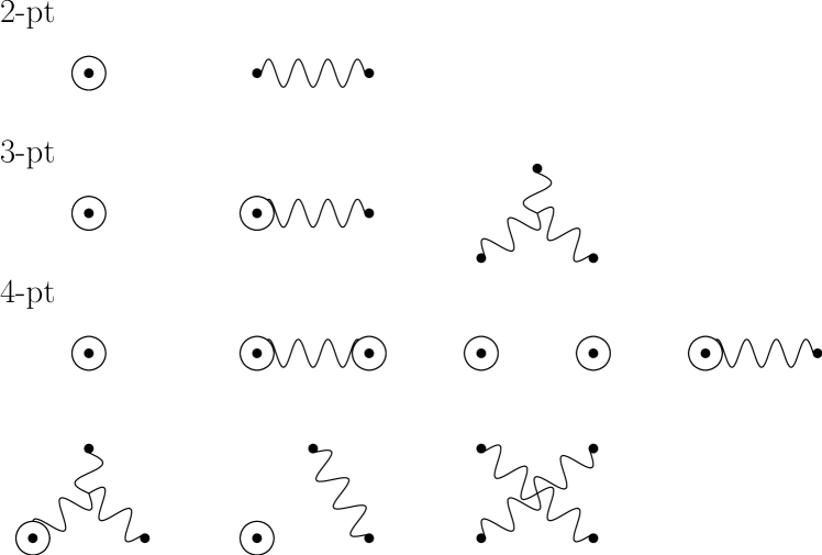
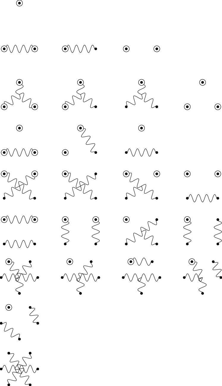
Appendix D The independence of the signal-to-noise ratio on the binning
In this section, we discuss the possible dependence of the signal-to-noise ratio, S/N, on the binning width . We first consider the case of power spectrum and then move to the bispectrum. Of course small inaccuracies arise when a coarse binning is used as the field varies across the bin. This is not the case we discuss here, instead we investigate whether the S/N explicitly depends on the binning to the lowest order.
For power spectrum, the Gaussian covariance scales with the binning as , while the trispectrum contribution does not depend on . The latter case is true for both the matter power spectrum case Eq. 6 and the Poisson model result Eq. 79. Suppose we change the binning in from to . For illustration purposes, let us take . When the binning is coarse grained by a factor of , the coarse-grained data vector is related to the original data vector as
| (88) |
i.e. an average over the neighbouring bins. For the sake of simplicity here we use a simple average instead of the phase-volume weighted one, but the discussion is still valid when a weighted mean is used. Correspondingly, the covariance matrix of the coarse-grained data vector, , is given by
| (89) | |||||
Therefore the coarse-grained covariance matrix is obtained by locally averaging the square block in the original matrix. In fact, the scalings of the Gaussian and non-Gaussian parts with respect to respect the averaging prescription Eq. 89. Clearly the non-Gaussian matrix elements are invariant with respect to binning up to the accuracy of the field represented by the binned value. When the Gaussian covariance matrix is coarse grained, the diagonal element of the coarse-grained one is obtained by averaging the diagonal elements and off-diagonal ones, which are zeroes. This is equivalent to simply averaging over the diagonal elements, and we get the scaling for the diagonal element.
We can expand the inverse of the covariance matrix perturbatively as
This series expansion is valid when the non-Gaussian part is smaller than the Gaussian one in some appropriate sense.
Plugging Eq. D into the signal-to-noise ratio , we can check the binning dependence term by term. Clearly the first term is invariant because although the number of bins is reduced by a factor of , the Gaussian precision matrix is enhanced by . Because the enhancement by a factor of in compensates the reduction in the number of rows in , the end result of is also invariant. By inspecting the perturbation series term by term, we conclude that the signal-to-noise for the power spectrum does not depend on the binning to the lowest order. This result was also stated in Ref. Takahashi et al. (2011).
We now consider the case of bispectrum. When the binning is rescaled by a factor of , say , the triangles in the bins are mapped into the triangle in the coarse-grained case. Here the triangle sides are in units of the fundamental mode . For example, when the binning is changed from to , the scalene triangles, [7][5][3], [7][5][4], [7][6][3], [7][6][4], [8][5][3], [8][5][4], [8][6][3], and [8][6][4] are mapped to . For triangles with some symmetries, i.e. the isosceles and equilateral triangles, the counting is slightly different. For example, for the equilateral triangle set [7,8][7,8][7,8], there are four distinct triangle sets [7][7][7], [7][7][8], [7][8][8], and [8][8][8] and they are mapped to . We should not include triangles such as [8][7][7] as it is identical to [7][7][8] and its inclusion would cause the covariance matrix to be singular. The symmetry factor is important for the consistency of counting. We comment that using a coarse binning for bispectrum is not very accurate for the bins with the smallest sides as triangles of many different shapes are mapped to a certain coarse-grained one. Yet for triangles of larger lengths, triangles are mapped to a triangle of similar shape by the coarse-graining transformation, and hence we expect that the coarse-grained field reflects the original one accurately.
The Gaussian bispectrum covariance scales with the binning as . The leading disconnected non-Gaussian contribution to the dark matter bispectrum covariance and also the non-Gaussian terms (Eq. 86) scale as and couple only triangles with at least one side equal to each other. On the other hand (Eq. 87) does not depend on and it couples all triangles. Again using Eq. D, we can check if the S/N changes when the binning is rescaled by a factor of , such as . For scalene triangles, the number of bins is reduced by a factor of 8, while is enhanced by a factor of 8, and hence it is invariant with respect to binning. For other shapes, such as the equilateral triangles, taking the symmetry factor into account, we can also show that is invariant. As the non-Gaussian term does not scale with , by reasoning similar to the case of power spectrum, we also deduce that this term is invariant under bin width rescaling. For the terms that scale as , the coupling is non-trivial in the covariance matrix, and it is hard to make an analytical argument. By considering some explicit examples for scalene, isosceles and equilateral triangles, we check that this particular scaling and coupling also result in the S/N invariant with respect to the binning width. Thus we have verified that the bispectrum S/N is invariant with respect to to the leading order.
References
- Percival et al. (2001) W. J. Percival et al. (2dFGRS), Mon. Not. Roy. Astron. Soc. 327, 1297 (2001), eprint astro-ph/0105252.
- Tegmark et al. (2004) M. Tegmark et al. (SDSS), Phys. Rev. D69, 103501 (2004), eprint astro-ph/0310723.
- Eisenstein et al. (2005) D. J. Eisenstein et al. (SDSS), Astrophys. J. 633, 560 (2005), eprint astro-ph/0501171.
- Cole et al. (2005) S. Cole et al. (2dFGRS), Mon. Not. Roy. Astron. Soc. 362, 505 (2005), eprint astro-ph/0501174.
- Tegmark et al. (2006) M. Tegmark et al. (SDSS), Phys. Rev. D74, 123507 (2006), eprint astro-ph/0608632.
- Anderson et al. (2014) L. Anderson et al. (BOSS), Mon. Not. Roy. Astron. Soc. 441, 24 (2014), eprint 1312.4877.
- Laureijs et al. (2011) R. Laureijs, J. Amiaux, S. Arduini, J. Auguères, J. Brinchmann, R. Cole, M. Cropper, C. Dabin, L. Duvet, A. Ealet, et al., ArXiv e-prints (2011), eprint 1110.3193.
- LSST Science Collaboration et al. (2009) LSST Science Collaboration, P. A. Abell, J. Allison, S. F. Anderson, J. R. Andrew, J. R. P. Angel, L. Armus, D. Arnett, S. J. Asztalos, T. S. Axelrod, et al., ArXiv e-prints (2009), eprint 0912.0201.
- Monaco (2016) P. Monaco (2016), eprint 1605.07752.
- Meiksin and White (1999) A. Meiksin and M. J. White, Mon. Not. Roy. Astron. Soc. 308, 1179 (1999), eprint astro-ph/9812129.
- Scoccimarro et al. (1999) R. Scoccimarro, M. Zaldarriaga, and L. Hui, Astrophys. J. 527, 1 (1999), eprint astro-ph/9901099.
- Smith (2009) R. E. Smith, Mon. Not. Roy. Astron. Soc. 400, 851 (2009), eprint 0810.1960.
- Takahashi et al. (2011) R. Takahashi, N. Yoshida, M. Takada, T. Matsubara, N. Sugiyama, I. Kayo, T. Nishimichi, S. Saito, and A. Taruya, Astrophys. J. 726, 7 (2011), eprint 0912.1381.
- Harnois-Déraps and Pen (2012) J. Harnois-Déraps and U.-L. Pen, MNRAS 423, 2288 (2012), eprint 1109.5746.
- Blot et al. (2015) L. Blot, P. S. Corasaniti, J.-M. Alimi, V. Reverdy, and Y. Rasera, Mon. Not. Roy. Astron. Soc. 446, 1756 (2015), eprint 1406.2713.
- Scoccimarro and Sheth (2002) R. Scoccimarro and R. K. Sheth, Mon. Not. Roy. Astron. Soc. 329, 629 (2002), eprint astro-ph/0106120.
- Sefusatti et al. (2006) E. Sefusatti, M. Crocce, S. Pueblas, and R. Scoccimarro, Phys. Rev. D74, 023522 (2006), eprint astro-ph/0604505.
- Scoccimarro et al. (2004) R. Scoccimarro, E. Sefusatti, and M. Zaldarriaga, Phys. Rev. D69, 103513 (2004), eprint astro-ph/0312286.
- Bertolini et al. (2016) D. Bertolini, K. Schutz, M. P. Solon, J. R. Walsh, and K. M. Zurek, Phys. Rev. D93, 123505 (2016), eprint 1512.07630.
- Mohammed et al. (2016) I. Mohammed, U. Seljak, and Z. Vlah, Submitted to: Mon. Not. Roy. Astron. Soc. (2016), eprint 1607.00043.
- Cooray and Hu (2001) A. Cooray and W. Hu, Astrophys. J. 554, 56 (2001), eprint astro-ph/0012087.
- Mohammed and Seljak (2014) I. Mohammed and U. Seljak, Mon. Not. Roy. Astron. Soc. 445, 3382 (2014), eprint 1407.0060.
- Matarrese et al. (1997) S. Matarrese, L. Verde, and A. F. Heavens, Mon. Not. Roy. Astron. Soc. 290, 651 (1997), eprint astro-ph/9706059.
- Rimes and Hamilton (2006) C. D. Rimes and A. J. S. Hamilton, Mon. Not. Roy. Astron. Soc. 371, 1205 (2006), eprint astro-ph/0511418.
- Hamilton et al. (2006) A. J. S. Hamilton, C. D. Rimes, and R. Scoccimarro, Mon. Not. Roy. Astron. Soc. 371, 1188 (2006), eprint astro-ph/0511416.
- de Putter et al. (2012) R. de Putter, C. Wagner, O. Mena, L. Verde, and W. J. Percival, JCAP 4, 019 (2012), eprint 1111.6596.
- Takada and Hu (2013) M. Takada and W. Hu, Phys. Rev. D87, 123504 (2013), eprint 1302.6994.
- Li et al. (2014) Y. Li, W. Hu, and M. Takada, Phys. Rev. D89, 083519 (2014), eprint 1401.0385.
- Sefusatti and Scoccimarro (2005) E. Sefusatti and R. Scoccimarro, Phys. Rev. D71, 063001 (2005), eprint astro-ph/0412626.
- Takada and Jain (2004) M. Takada and B. Jain, Mon. Not. Roy. Astron. Soc. 348, 897 (2004), eprint astro-ph/0310125.
- Kayo et al. (2013) I. Kayo, M. Takada, and B. Jain, MNRAS 429, 344 (2013), eprint 1207.6322.
- Sato and Nishimichi (2013) M. Sato and T. Nishimichi, Phys. Rev. D87, 123538 (2013), eprint 1301.3588.
- Angulo et al. (2008) R. Angulo, C. M. Baugh, C. S. Frenk, and C. G. Lacey, Mon. Not. Roy. Astron. Soc. 383, 755 (2008), eprint astro-ph/0702543.
- Feldman et al. (1994) H. A. Feldman, N. Kaiser, and J. A. Peacock, ApJ 426, 23 (1994), eprint astro-ph/9304022.
- Fry (1984) J. N. Fry, ApJ 279, 499 (1984).
- Goroff et al. (1986) M. H. Goroff, B. Grinstein, S.-J. Rey, and M. B. Wise, ApJ 311, 6 (1986).
- Bernardeau et al. (2002) F. Bernardeau, S. Colombi, E. Gaztañaga, and R. Scoccimarro, Phys. Rep. 367, 1 (2002), eprint arXiv:astro-ph/0112551.
- Rasera et al. (2014) Y. Rasera, P.-S. Corasaniti, J.-M. Alimi, V. Bouillot, V. Reverdy, and I. Balmès, Mon. Not. Roy. Astron. Soc. 440, 1420 (2014), eprint 1311.5662.
- Spergel et al. (2007) D. N. Spergel, R. Bean, O. Doré, M. R. Nolta, C. L. Bennett, J. Dunkley, G. Hinshaw, N. Jarosik, E. Komatsu, L. Page, et al., ApJs 170, 377 (2007), eprint astro-ph/0603449.
- Lewis et al. (2000) A. Lewis, A. Challinor, and A. Lasenby, ApJ. 538, 473 (2000), eprint arXiv:astro-ph/9911177.
- Teyssier (2002) R. Teyssier, A&A 385, 337 (2002), eprint astro-ph/0111367.
- Chan et al. (2012) K. C. Chan, R. Scoccimarro, and R. K. Sheth, Phys. Rev. D 85, 083509 (2012), eprint arXiv:1201.3614.
- Taylor et al. (2013) A. Taylor, B. Joachimi, and T. Kitching, MNRAS 432, 1928 (2013), eprint 1212.4359.
- Scoccimarro et al. (1998) R. Scoccimarro, S. Colombi, J. N. Fry, J. A. Frieman, E. Hivon, and A. Melott, ApJ 496, 586 (1998), eprint arXiv:astro-ph/9704075.
- Press et al. (2007) W. H. Press, S. A. Teukolsky, W. T. Vetterling, and B. P. Flannery, Numerical Recipes 3rd Edition: The Art of Scientific Computing (Cambridge University Press, New York, NY, USA, 2007), 3rd ed., ISBN 0521880688, 9780521880688.
- Xu et al. (2015) Y. Xu, X. Wang, and X. Chen, Astrophys. J. 798, 40 (2015), eprint 1410.7794.
- Welling et al. (2016) Y. Welling, D. van der Woude, and E. Pajer (2016), eprint 1605.06426.
- Xu et al. (2016) Y. Xu, J. Hamann, and X. Chen, ArXiv e-prints (2016), eprint 1607.00817.
- Tegmark et al. (1997) M. Tegmark, A. Taylor, and A. Heavens, Astrophys. J. 480, 22 (1997), eprint astro-ph/9603021.
- Hartlap et al. (2007) J. Hartlap, P. Simon, and P. Schneider, Astron. Astrophys. 464, 399 (2007), eprint astro-ph/0608064.
- Anderson (2003) T. W. Anderson, An Introduction to Multivariate Statistical Analysis, 3rd Edition (Wiley-Interscience, New York, 2003).
- Blot et al. (2016) L. Blot, P. S. Corasaniti, L. Amendola, and T. D. Kitching, Mon. Not. Roy. Astron. Soc. 458, 4462 (2016), eprint 1512.05383.
- Jenkyns and Muller (2000) T. Jenkyns and E. Muller, The American Mathematical Monthly 107, 634 (2000).
- Rimes and Hamilton (2005) C. D. Rimes and A. J. S. Hamilton, Mon. Not. Roy. Astron. Soc. 360, L82 (2005), eprint astro-ph/0502081.
- Neyrinck et al. (2006) M. C. Neyrinck, I. Szapudi, and C. D. Rimes, Mon. Not. Roy. Astron. Soc. 370, L66 (2006), eprint astro-ph/0604282.
- Lee and Pen (2008) J. Lee and U.-L. Pen, Astrophys. J. 686, L1 (2008), eprint 0807.1538.
- Coles and Jones (1991) P. Coles and B. Jones, MNRAS 248, 1 (1991).
- Neyrinck et al. (2009) M. C. Neyrinck, I. Szapudi, and A. S. Szalay, ApJL 698, L90 (2009), eprint 0903.4693.
- Carron and Neyrinck (2012) J. Carron and M. C. Neyrinck, ApJ 750, 28 (2012), eprint 1201.1444.
- Repp et al. (2015) A. Repp, I. Szapudi, J. Carron, and M. Wolk, MNRAS 454, 3533 (2015), eprint 1506.00083.
- Kayo and Takada (2013) I. Kayo and M. Takada (2013), eprint 1306.4684.
- Feldman et al. (2001) H. A. Feldman, J. A. Frieman, J. N. Fry, and R. Scoccimarro, Phys. Rev. Lett. 86, 1434 (2001), eprint astro-ph/0010205.
- Scoccimarro et al. (2001) R. Scoccimarro, H. A. Feldman, J. N. Fry, and J. A. Frieman, Astrophys. J. 546, 652 (2001), eprint astro-ph/0004087.
- Verde et al. (2002) L. Verde et al., Mon. Not. Roy. Astron. Soc. 335, 432 (2002), eprint astro-ph/0112161.
- Gil-Marín et al. (2015) H. Gil-Marín, J. Noreña, L. Verde, W. J. Percival, C. Wagner, M. Manera, and D. P. Schneider, Mon. Not. Roy. Astron. Soc. 451, 539 (2015), eprint 1407.5668.
- Jing and Boerner (2004) Y. P. Jing and G. Boerner, Astrophys. J. 607, 140 (2004), eprint astro-ph/0311585.
- Gaztañaga and Scoccimarro (2005) E. Gaztañaga and R. Scoccimarro, MNRAS 361, 824 (2005), eprint astro-ph/0501637.
- Wang et al. (2004) Y. Wang, X.-H. Yang, H. J. Mo, F. C. van den Bosch, and Y.-Q. Chu, Mon. Not. Roy. Astron. Soc. 353, 287 (2004), eprint astro-ph/0404143.
- Marín (2011) F. Marín, ApJ 737, 97 (2011), eprint 1011.4530.
- Marín et al. (2013) F. A. Marín, C. Blake, G. B. Poole, C. K. McBride, S. Brough, M. Colless, C. Contreras, W. Couch, et al., MNRAS 432, 2654 (2013), eprint 1303.6644.
- Slepian et al. (2015) Z. Slepian et al. (2015), eprint 1512.02231.
- Guo et al. (2016) H. Guo et al. (2016), eprint 1608.03660.
- Fry and Gaztañaga (1993) J. N. Fry and E. Gaztañaga, ApJ 413, 447 (1993), eprint arXiv:astro-ph/9302009.
- Baldauf et al. (2012) T. Baldauf, U. Seljak, V. Desjacques, and P. McDonald, Phys. Rev. D 86, 083540 (2012), eprint arXiv:1201.4827.
- Hamaus et al. (2014) N. Hamaus, B. D. Wandelt, P. M. Sutter, G. Lavaux, and M. S. Warren, Physical Review Letters 112, 041304 (2014), eprint 1307.2571.
- Chan et al. (2014) K. C. Chan, N. Hamaus, and V. Desjacques, Phys. Rev. D 90, 103521 (2014), eprint 1409.3849.
- Clampitt et al. (2016) J. Clampitt, B. Jain, and C. Sánchez, MNRAS 456, 4425 (2016), eprint 1507.08031.
- Kitaura et al. (2016) F.-S. Kitaura, C.-H. Chuang, Y. Liang, C. Zhao, C. Tao, S. Rodríguez-Torres, D. J. Eisenstein, H. Gil-Marín, J.-P. Kneib, C. McBride, et al., Physical Review Letters 116, 171301 (2016), eprint 1511.04405.
- Hamaus et al. (2016) N. Hamaus, A. Pisani, P. M. Sutter, G. Lavaux, S. Escoffier, B. D. Wandelt, and J. Weller, Physical Review Letters 117, 091302 (2016), eprint 1602.01784.
- Chiang et al. (2002) L.-Y. Chiang, P. Coles, and P. Naselsky, MNRAS 337, 488 (2002), eprint astro-ph/0207584.
- Wolstenhulme et al. (2015) R. Wolstenhulme, C. Bonvin, and D. Obreschkow, ApJ 804, 132 (2015), eprint 1409.3007.
- Eggemeier et al. (2015) A. Eggemeier, T. Battefeld, R. E. Smith, and J. Niemeyer, MNRAS 453, 797 (2015), eprint 1504.04036.
- Mehrem (2011) R. Mehrem (2011), eprint arXiv:0909.0494.
- Abramowitz and Stegun (1964) M. Abramowitz and I. A. Stegun, Handbook of Mathematical Functions with Formulas, Graphs, and Mathematical Tables (Dover Publications, New York, 1964).
- Chan and Scoccimarro (2012) K. C. Chan and R. Scoccimarro, Phys. Rev. D 86, 103519 (2012), eprint arXiv:1204.5770.
- Peebles (1980) P. J. E. Peebles, The Large-Scale Structure of the Universe (Princeton University Press, New Jersey, 1980).