VoIgt profile Parameter Estimation Routine (viper): H i photoionization rate at
Abstract
We have developed a parallel code called “VoIgt profile Parameter Estimation Routine (viper)” for automatically fitting the H i Ly- forest seen in the spectra of QSOs. We obtained the H i column density distribution function (CDDF) and line width () parameter distribution for using spectra of 82 QSOs obtained using Cosmic Origins Spectrograph and viper. Consistency of these with the existing measurements in the literature validate our code. By comparing this CDDF with those obtained from hydrodynamical simulation, we constrain the H i photoionization rate () at in four redshift bins. The viper, together with the Code for Ionization and Temperature Evolution (cite) we have developed for gadget-2, allows us to explore parameter space and perform minimization to obtain . We notice that the parameters from the simulations are smaller than what are derived from the observations. We show the observed parameter distribution and vs scatter can be reproduced in simulation by introducing sub-grid scale turbulence. However, it has very little influence on the derived . The obtained here, , is in good agreement with those derived by us using flux based statistics in the previous paper. These are consistent with the hydrogen ionizing ultra-violet (UV) background being dominated mainly by QSOs without needing any contribution from the non-standard sources of the UV photons.
keywords:
cosmological parameters - cosmology: observations-intergalactic medium-QSOs: absorption lines-ultraviolet: galaxies1 Introduction
The Ly- forest absorption seen in the spectra of the luminous distant QSOs is one of the most sensitive tools to study the physical conditions of the intergalactic medium (IGM). In hierarchical structure formation models, Ly- forest is thought to arise from the fluctuations in the cosmic density field (Bi et al., 1992; Bi, 1993; Bi & Davidsen, 1997; Croft et al., 1997, 1998). The strength and width of the Ly- absorption lines can be used to trace the ionization and thermal state of the neutral hydrogen (H i) in the IGM. Thus observations of the Ly- forest have regularly been used to constrain cosmological and astrophysical parameters related to IGM physics.
Various statistics are used in the literature to constrain cosmological and astrophysical parameters from the Ly- forest observations. These statistics are broadly divided into two cases. In the first case, Ly- transmitted flux is treated as a continuous field quantity. In particular, the mean flux, the flux probability distribution function (PDF) and the flux power spectrum (PS) have been used to constrain cosmological parameters such as , , and (McDonald et al., 2000; Phillips et al., 2001; Choudhury et al., 2001; Tegmark et al., 2004; Viel et al., 2004a, b; McDonald et al., 2005; Seljak et al., 2006; Viel & Haehnelt, 2006; Viel et al., 2006, 2009), thermal history parameters111The thermal state of the IGM is described by the effective equation of state parameterized by the mean IGM temperature () and the slope (). (Zaldarriaga et al., 2001; Bolton et al., 2008; Lidz et al., 2010; Becker et al., 2011; Calura et al., 2012; Garzilli et al., 2015) and H i photoionization rate (; Rauch et al., 1997; Meiksin & White, 2004; Bolton & Haehnelt, 2007; McQuinn et al., 2011; Becker & Bolton, 2013; Pontzen et al., 2014; Gaikwad et al., 2017). Constraining such quantities by comparing flux statistics between observations and simulations are relatively easier and are frequently used in the high- () studies. In the second case, Ly- forest is decomposed into multiple Voigt profiles. The line width distribution function calculated from Voigt profile fitting is sensitive to the thermal history and the energy injected by various astrophysical processes in the form of heat and turbulent motions in the IGM (Schaye et al., 1999, 2000; McDonald et al., 2001; Davé & Tripp, 2001). Similarly, the column density distribution function (CDDF) calculated from Voigt profile decomposition is sensitive to (Cooke et al., 1997; Kollmeier et al., 2014; Shull et al., 2015; Gurvich et al., 2016) and cosmological parameters (Storrie-Lombardi et al., 1996; Penton et al., 2000; Shull et al., 2012). While statistics based on parameters obtained using Voigt profile fitting are useful in deriving thermal history and equation of state of the IGM, the Voigt profile decomposition is usually a time consuming process. Therefore, a large parameter space exploration in simulations is usually difficult.
To constrain using CDDF at low- (i.e., ), the UV spectrograph on space telescope is needed for the Ly- forest observations. Thanks to Cosmic Origins Spectrograph onboard Hubble Space Telescope (hereafter hst-cos) we have good quality observations of the low- Ly- forest. These observations are used to place good constraints on (Kollmeier et al., 2014; Shull et al., 2015; Gaikwad et al., 2017). Previous measurement of using CDDF by Kollmeier et al. (2014, hereafter K14) and Shull et al. (2015, hereafter S15) are conflicting. S15 found a factor smaller than K14222The errorbars on are not evaluated systematically in either K14 or S15.. Note that both used the same hst-cos data but different cosmological simulations. Recently Gaikwad et al. (2017) (hereafter Paper-I) used same hst-cos data but different statistics namely flux PDF and flux PS to constrain with appropriate errorbars333S15 analysis is based on ENZO which uses adaptive mesh refinement (AMR) technique. K14 used smoothed particle hydrodynamic gadget-3 code. Whereas, Paper-I used smoothed particle hydrodynamic gadget-2 code coupled with Code for Ionization and Temperature Evolution (cite) see §4 for more detail. This allowed us to explore the parameter space in detail.. In contrast to K14 and S15, Paper-I varied as a free parameter, minimize the for the two statistics and calculated appropriate statistical and systematic uncertainties in using covariance matrices for a range of IGM thermal histories. The measurements and its evolution obtained in Paper-I is found to be consistent with those from S15.
In this paper we measure the and associated errors at low- using CDDF by varying as a free parameter. The basic idea behind constraining is to calculate the between the observed CDDF, , and the CDDF, , calculated by modeling the Ly- forest in a cosmological simulation. The corresponding to minimum value of (i.e. ) gives the best fit whereas the associated statistical error is obtained by calculating the parameter values corresponding to (Press et al., 1992). The modeling of the Ly- forest is relatively simple (Cen et al., 1994; Zhang et al., 1995; Miralda-Escudé et al., 1996; Hernquist et al., 1996) and well understood as they probe mildly non-linear densities of the IGM ( at , see Table 2 in Paper-I). However, at low- Ly- absorption could originate from the extended circumgalactic medium of star forming galaxies. The free parameter could be degenerate with thermal history parameters such as mean IGM temperature and slope of equation of state (as shown at by Bolton et al., 2005; Bolton & Haehnelt, 2007; Faucher-Giguère et al., 2008). In Paper-I, we developed a module named “Code for Ionization and Temperature Evolution (cite)” that allows one to probe the wide range of thermal history and easily. Using cite, we varied the thermal history parameters at high- () and evolved the IGM temperature up to . As shown in Paper-I, the thermal history parameters at low- are found to be very similar and even if the initial parameters and at are quite different. This implies that the derived at low- are not very sensitive to the thermal history of the IGM at .
In order to obtain the CDDF, each Ly- absorption is usually decomposed into multiple Voigt profile components. Each Voigt profile is defined by free parameters i.e., line center (), H i column density () and line width parameter (). The manual Voigt decomposition of the large number () of simulated Ly- forest is laborious and time consuming. Furthermore, the criteria used to fit the number of components () to a given identified Ly- absorption is subjective and need not be unique. Although there are several Voigt profile fitting codes available in the literature like vpfit444http://www.ast.cam.ac.uk/~rfc/vpfit.html, alis (Cooke et al., 2014), gvpfit (Bainbridge & Webb, 2016) it will be invaluable to have a tailor made automatic module that will identify Ly- absorption regions and fit them with multiple component Voigt profiles where the best fit parameters of the individual components and the minimum number of required components are determined through objective criterion.
We have developed a parallel processing module “VoIgt profile Parameter Estimation Routine” (viper) to fit the Ly- forest with multiple Voigt profiles automatically. In viper, the blended and saturated features are fitted simultaneously with multi-component Voigt profiles. An objective criteria based on information theory is used to find the number of Voigt profiles needed to describe the Ly- forest. The parallel and automated nature of viper allows us to simultaneously fit large number of simulated spectra and to explore a wide parameter space efficiently. For consistency, we used the same code for analyzing the observed and simulated spectra. We calculated CDDF by consistently taking into account the redshift path length and the incompleteness of the observed sample. We show CDDF and line width distribution obtained for observed data using viper matches very well with those from Danforth et al. (2016).
The paper is organized as follows. In §2 and §4 we explain the hst-cos data and cosmological simulation used in this work. §3 describes our module viper that automatically fits Voigt profiles to the Ly- forest. In §5 we match observed CDDF with model CDDF to constrain in different redshift bins defined in Paper-I. Finally we summarize our results in §6. Throughout this work we use flat CDM cosmology with parameters reported by Planck Collaboration et al. (2015). All the distances are expressed in comoving co-ordinates unless and otherwise mentioned. The H i photoionization rate in units of is denoted by .
2 HST-COS QSO ABSORPTION SPECTRA
We used publicly available hst-cos science data product555https://archive.stsci.edu/prepds/igm/ that consists of a sample of low redshift Ly- forest spectra towards 82 UV bright QSOs performed by Danforth et al. (2016, hereafter D16). These QSOs are distributed in the redshift range to . The sample covers the Ly- forest in the redshift range with a velocity resolution of (full width at half maximum). The median signal-to-noise ratio (SNR) per pixel varies from to for different sightlines.
D16 fitted the continuum to each spectrum and identified several thousand absorption line features that consists of Ly- lines, higher order Ly-series lines, metal lines from the IGM and the interstellar medium (ISM) of our Galaxy. As a part of the hst-cos science data product, D16 fitted each absorption feature with multiple component Voigt profiles and provided a table that contains line identifications (type of the specie and rest wavelength of the transition), redshift of the absorption system, column density, doppler- parameter, equivalent width (along with associated fitting errors) and significance level of the absorption line detection. In this work we refer to their Ly- line catalog as “D16 line catalog”.
As in Paper-I, we divided the sample into 4 different redshift bins (we denote them by roman numerals I, II, III and IV respectively) . The size and center of the lowest redshift bin is chosen in a way that avoids the contamination by geo-coronal line emission at . There are total and lines of sight in the redshift bins I, II, III and IV respectively. Apart from the intervening Ly- lines all other lines in the Ly- forest are treated as contamination in our spectra. We replace all other lines except Ly- lines by the continuum added with a Gaussian random noise (see Fig. 2 in Paper-I, ). We use these clean spectra for further analysis.
3 Automatic Voigt profile fitting code
In this section we describe our automated Voigt profile fitting procedure “VoIgt profile Parameter Estimation Routine” (viper). The same code has been used to fit the observed and simulated Ly- forest spectra to constrain in §5 from CDDF. The algorithm is broadly divided into 3 steps; first we identify the absorption lines and region bracketing these lines, next in these regions we fit as many Voigt components as necessary based on an objective criteria. In the final step we accept the Voigt profile fit for a line based on a significance level of the fit. We now discuss each step in detail below.
-
1.
Line and region identification : Following Schneider et al. (1993) and D16, first we estimate the “crude significance level” (hereafter CSL) to identify the lines,
(1) where and are “equivalent width vector” and “line-less error vector” respectively. The CSL defined in this way has the advantage that the unresolved features are unlikely to be identified as lines (see Schneider et al., 1993, for details). and are obtained by convolving the normalized flux and line-less error (i.e., error on flux if absorption lines were absent), respectively, with a representative line profile (see §2.3 of D16). The representative line profile is a convolution of Gaussian (of a Doppler parameter of ) with hst-cos line spread function (LSF). We repeated the procedure with different values of the doppler to incorporate any missing narrower, broader and blended lines. The second panel from the top in Fig. 1 shows the CSL estimated for the spectrum shown in the top panel. Initially we identified all the lines with maxima satisfying shown by red stars in second panel of Fig. 1666The cutoff used in this work is smaller than that used by D16 (). This results in more number of identified lines in our initial line catalog as compared to D16. However, in the final step most of the extra identified lines at lower significance level are rejected.. Next we find a threshold on either side of the maxima to enclose the line in a region. A minimum is accepted as a threshold if . A minimum with indicates that the lines are blended hence we search for the next minimum until we meet the condition to accept it as a threshold. We then merge the overlapping regions (if any) into one bigger region for blended lines (e.g., see the yellow shaded region in second panel of Fig. 1). This procedure allows us to identify and fit the blended lines simultaneously.

Figure 1: Illustration of different steps in the automatic Voigt profile fitting procedure used in viper. Top panel shows a portion of the observed hst-cos spectrum along the sightline towards QSO PKS1302-102. Second panel from top shows the estimation of crude significance level (CSL) using the Eq.1 (for km s-1). All the identified peaks with (magenta dashed line) are shown by red stars. The identified regions enclosing the peaks are shown by black dashed vertical lines. Overlapping regions are merged accordingly to fit blended lines simultaneously (see yellow shaded region). All the identified regions are fitted with Voigt profile as shown in the third panel from top. The number of components used to fit the region is decided using AICC and demanding (see §3). Rigorous significance level (RSL) for each fitted line is calculated using Eq.4. Bottom panel shows the accepted fit with the . -
2.
Voigt profile fitting : In this step we fit each identified region by multiple Voigt profiles. Voigt profile, convolution of Gaussian with Lorentzian, is a real part of the “Faddeeva function” (Armstrong, 1967),
(2) where is the error function, is Voigt profile and is imaginary part of Faddeeva function. We used wofz777http://ab-initio.mit.edu/wiki/index.php/Faddeeva_Package function in python’s scipy package to compute Voigt profile. We convolve this Voigt profile with the appropriate hst-cos lsf before performing minimization888We assumed that the observed fluxes in different pixels are uncorrelated. hst-cos lsf is not a Gaussian (http://www.stsci.edu/hst/cos/performance/spectral_resolution/). This function is slightly asymmetric around the center and has extended wings.. For minimization, we used leastsq999https://docs.scipy.org/doc/scipy-0.18.1/reference/generated/scipy.optimize.leastsq.html function in python’s scipy package. If , , are observed flux, error in the observed flux and fitted Ly- flux respectively then we minimize the function in leastsq routine. The fit parameters are allowed to vary over the range , and bounds are set by the wavelength of the region. We set initial guess values for lines in a given region by fitting individual line in that region with a Gaussian. Note that in the previous step each identified line is enclosed in two CSL minima hence we can fit each line separately. However initial guess values for any additional line required by the information criteria (explained below) are set randomly in the region.
A criteria based on information theory, Akaike Information Criteria with Correction (AICC) (Akaike, 1974; Liddle, 2007; King et al., 2011) is used to assess the optimum number of Voigt profile components required for an acceptable fit. If is the number of parameters in a model used to fit the data with pixels, then the AICC is given by,
(3) The first term on right-hand side is a measure of loss of information while describing the data with a model. The second term in right-hand side quantifies the complexity of the model. Thus AICC incorporates the trade-off between loss of information and complexity of the model. We assign a model to be the best fit model over the previously assigned best fit model if AICC is lower by at least 5 (Jeffreys, 1961). Since only the relative difference in the AICC values is important, according to Jeffreys (1961) AICC = 5 is considered as the strong evidence against the weaker model. Fig. 2 illustrates our method of choosing a best fit model. Black points in left-hand panel of the Fig. 2 are data points which we want to fit by Voigt profile model. We fitted the data with different number of (say ) Voigt profiles. The resulting AICC and for each model as a function of is shown by star and circle respectively in the right-hand panel of the Fig. 2.

Figure 2: Left-hand panel shows the three different Voigt profile fits with and (green dot-dashed, red continuous and blue dashed lines respectively) fitted to the observed data (black circle). The spectrum is shown in the velocity scale defined with respect to the redshift of the strongest line center. Right-hand panel shows the corresponding variation of AICC (stars) and (magenta circles) for 5 different models. For legibility fits with (gray star points) are not shown in left-hand panel. For , the remains constant whereas AICC increases due to the second term on right-hand side of Eq.3. The best fit model corresponds to the minimum AICC (where is also achieved) i.e., shown by black arrow in right-hand panel and red solid line in left-hand panel. For the model is less complex but the () between model and data is large (see green curve in left-hand panel) resulting in a larger AICC value101010The reduced is given by, where is number of pixels in the given region (left-hand panel of Fig. 2), is number of free parameters where factor 3 accounts for the number of free parameters in each Voigt component (, and ).. Whereas, for , the () is small (see blue curve in left-hand panel) but with increasing the complexity of the model increases and hence AICC also increases. It is interesting to note that the remains nearly constant for whereas AICC systematically increases for . A model simply based on minimization, thus would be degenerate for . The minimum AICC occurs for (black arrow showing red star in right-hand panel) which shows trade-off between goodness-of-fit () and complexity of the model. The corresponding best fit model is shown by red curve in left-hand panel. Thus for minimum AICC, is also close to and hence we chose it to be the best fit model. In the third panel from top of Fig. 1, we show the results of fitting each region with as many Voigt components as necessary for the minimum AICC and .
-
3.
Significance level of fitted lines : Initially we fitted the lines that are identified using a simple approximation of “Crude Significance Level”. However, we used a “Rigorous Significance Level” (hereafter RSL) formula (Keeney et al., 2012) to include the lines in the final line catalog as given below,
(4) where, is width (in pixels) of discrete region over which equivalent width is calculated, , is width (in ) of the discrete region, is the fractional area of the hst-cos lsf contained within the region of integration, takes care of the fact that noise property may not be purely Poissonian, is signal to noise ratio per pixel, signal to noise ratio average over discrete region containing pixels. We used the parametric form of given by Keeney et al. (2012, their Eq. 4, Eq. 7 to Eq. 11 with parameters given in Table.1 for the coadded data).
To avoid the spurious detection, we retain only feature measured with in the final line catalog. Other features are excluded from further analysis. Using this criteria, we find that the number of identified lines with to be fitted by viper (1277 H i Ly- lines) are similar to those of D16 (1280 H i Ly- lines)111111The total number of identified lines above completeness limit (i.e., 13.6) in viper and D16 line catalog is 533 and 522 respectively.. In the third panel from top of Fig. 1, we show the RSL for each fitted component above the line. Bottom panel of Fig. 1 shows that the final accepted Voigt profile fit that contains only those components which have .
The comparison of Voigt profile fit of viper with that of D16 method is illustrated in Fig. 3. The fit from viper and D16 method is shown by solid red and dashed blue line respectively. The line centers of components fitted by viper and D16 method are shown by solid red and dashed blue vertical ticks respectively. For viper the reduced is small as compared to that for the components obtained by D16. The top row shows the example where viper fit (in terms of number of component and the values of fitted parameter along with the errorbar) matches well with D16 fit. In most situations the fitted parameters from viper matched well with those from D16 within errors. In few cases viper fitted data better than D16 method (bottom row of Fig. 3) in terms of reduced . We fitted all the observed spectra using viper and form a line catalog “viper catalog” (see Appendix for details). It should be noted that unlike D16, viper does not fit higher order Lyman series lines (e.g. Ly-, Ly-) simultaneously for an accurate measurement of in the case of saturated Ly- lines. However, we show in the next section that the differences in CDDF and line width distributions from “viper catalog” and “D16 catalog” are very small.

Figure 3: Comparison of Voigt profiles fitted using our procedure with those of D16 for four different regions in our sample. Black filled circles, the solid red line and the dashed blue line are observed data points, the best fit profile from viper and from D16 respectively. The spectra are shown in the velocity scale defined with respect to the redshift of the strongest component. Blue dashed and red continuous vertical ticks show the location of identified components by D16 and viper respectively. The residual between observed data and fitting from D16 (open blue stars) and viper (red filled circles) model are shown in the corresponding lower panel. In majority of cases ( percent, like upper row panels) our parameters within errors match with those from D16. However, for some cases our fit to the data using AICC (i.e., using criteria AICC 5, see text for details) is found to be better (lower row panels). In all four cases shown above our is better than the corresponding from D16. 3.1 Column density distribution function (CDDF):
Column density distribution function, , describes the number of absorption lines in the column density range and d and in the redshift range to . For a singular isothermal density profile of Ly- absorbers, the H i photoionization rate can be inferred from H i CDDF as (Schaye, 2001; Shull et al., 2012),
(5) We take into account the completeness of the sample while calculating the redshift path length as a function of . Following D16, we calculate the CDDF in bins with centers at and width d .

Figure 4: Left-hand panel illustrates our redshift path length calculation for sightline towards QSO H1821+643. Top, middle and lower left-hand panels show the flux, SNR per pixel and equivalent width vector respectively. Equivalent width vector is calculated for RSL = 4 in Eq.4. The limiting equivalent width (), estimated from the curve of growth, corresponding to is shown by horizontal black dashed line in the bottom panel. The redshift path length, , for this sightline is the redshift covered by region . The total redshift path length is sum of the measured along all QSO sightlines. Right-hand panel shows (blue curve) the total redshift path length as a function of (known as sensitivity curve). The completeness limit for the sample is (shown by blue arrow). The fractional area in a given bin, , is area under the blue curve in the corresponding bin (shown by blue text) that is used in CDDF calculation. Left-hand panel in Fig. 4 illustrates the procedure we adopt for calculating the redshift path length. The top, middle and lower sub-panels show the flux , SNR per pixel and equivalent width vector respectively for a sightline towards QSO H1821+643. To calculate the equivalent width vector , Eq.4 is rearranged and solved for by taking RSL=4 and (corresponds velocity resolution) for each pixel. Next we calculate limiting equivalent width from curve of growth () for different values of . As an example we show for by black dashed horizontal line in bottom panel of Fig. 4. The redshift path length for this sightline (shown by blue curve in bottom panel) is the sum of redshift range for which . The total redshift path length covered in the observed sample is a sum of all the redshift path length in individual sightlines. The total redshift path length is then plotted as a function of (‘Sensitivity curve’) as shown in right-hand panel of Fig. 4. The completeness limit for the sample is (shown by blue arrow) i.e., the lines with are always detectable over the entire observed wavelength range for the full sample. The fractional area d in Eq.5 is calculated by integrating the sensitivity curve in the corresponding d bin. We shall refer to the CDDF obtained for our fitted parameters (over the redshift range ) in this way as “viper CDDF”.
In the left-hand panel of Fig. 5, we compared the viper CDDF with CDDF given in Table.5 of D16 (also S15) and CDDF calculated from D16 line catalog. The CDDF given in Table.5 of D16 is calculated from H i absorbers in the redshift range whereas CDDF calculated from D16 line catalog contains H i absorbers in the redshift range . We used our redshift path length estimation for CDDF calculation from D16 line catalog. The viper and the D16 line catalog CDDFs are consistent with each other within except at high and low bins. The median from viper and D16 is and respectively. The two sample KS test -value between the distribution of viper and D16 line catalog is 0.83. The consistency between viper CDDF and D16 line catalog CDDF suggests that the number of components identified by viper in different d bins are similar to those from D16 line catalog. Whereas, the agreement between viper CDDF and CDDF from D16 paper indicates that our redshift path calculation is consistent with that from D16 paper.
We notice occasional component differences when the Ly- line is heavily saturated between D16 and our viper fits. Unlike D16, viper does not include simultaneous fitting of Ly- line and higher order Lyman series lines (such as Ly-, Ly-). This could be the reason for minor mismatch of CDDF in the bins and . Thus minor differences one notices in high and intermediate bins in observed CDDF can be attributed to the differences in the multi-component fitting procedure in particular to the way the total number of components fitted to a given identified absorption region. However, there is an overall good agreement between CDDF derived by D16 and viper.
In the right-hand panel of Fig. 5, we compared the doppler- parameter distribution from viper catalog (red curve with shaded region) and D16 line catalog (black dashed line with error bars)121212In left-hand panel of Fig. 5, we compare our CDDF with that from D16 line catalog () and D16 paper (). However, in right-hand panel of Fig. 5, we compare our parameter distribution (i.e. in the redshift range ) with that from D16 catalog only as the parameter distribution is not available in D16 paper.. In both distributions the errors are assumed to be poisson distributed. The median value of parameter from viper and D16 is km s-1and km s-1respectively. The two sample KS test -value between the parameter distribution of viper and D16 line catalog is 0.41. Thus the two distributions are consistent with each other validating the consistency between viper and D16 line fitting methods.

4 Simulation
In this section we discuss the simulations used to generate the Ly- forest that will be subsequently used to constrain in §5. We used publicly available smoothed particle hydrodynamic code gadget-2131313http://wwwmpa.mpa-garching.mpg.de/gadget/ (Springel, 2005) to generate density and velocity field in a periodic box of size cMpc. The initial conditions were generated at by using the publicly available 2lpt141414http://cosmo.nyu.edu/roman/2LPT/ (Scoccimarro et al., 2012) initial conditions code. Radiative heating and cooling processes are not incorporated in default version of gadget-2. We used our module “Code for Ionization and Temperature Evolution” (hereafter cite) to evolve the temperature of the IGM in the post-processing step of the gadget-2. We refer reader to Paper-I where cite is discussed in detail.
In Paper-I, we showed the consistency of our method of evolving IGM temperature in gadget-2+cite with other low- simulations in the past (Davé et al., 2010; Smith et al., 2011; Tepper-García et al., 2012) using 3 metrics (i) the thermal history parameters at , (ii) distribution of baryons in different regions of the phase diagram and (iii) column density () vs overdensity () relationship. We used model given in Table 3 of Paper-I to calculate column density distribution function. In this model we evolve the equation of state of the IGM from K and at to . The final thermal history parameters at low redshift for this model are , , ,
Once we have calculated temperature of the gadget-2 particles we generate the Ly- forest by shooting random lines of sight through simulation box (Choudhury et al., 2001; Padmanabhan et al., 2015, Paper-I). To account for the possible redshift evolution of the structures, we generated Ly- forest from the simulation box at an for comparison with observations. The basic steps are as follows,
-
•
Using sph smoothing kernel, the density, velocity and temperature are calculated on the grids along the sightline.
-
•
Assuming photoionization equilibrium with ultra-violet background (hereafter UVB), the number density of neutral hydrogen () is calculated along the sightline.
-
•
We treat H i photoionization rate () as a free parameter in our analysis. For a given value of , Ly- optical depth is calculated at each pixel from the field and by properly accounting for peculiar velocity, thermal width and natural width effects on the line profile.The transmitted flux is then given by .
-
•
The velocity separation of pixels in the simulated spectra is whereas observed spectra are at velocity resolution. We linearly interpolate the simulated spectra to match with observed velocity resolution.
-
•
The line spread function of hst-cos is skewed and has extended wings. We account for this effect by convolving the simulated spectra with hst-cos lsf. Finally we add the Gaussian random noise to the simulated spectra with SNR same as the observed spectra.
We generated number of Ly- forest spectra at redshift to account for the variance in the model CDDF (for similar method see Rollinde et al., 2013, Paper-I). Here, is number of observed spectra at the redshift of interest and is number of mock samples. It should be noted that the dynamical impact of diffuse IGM pressure is not modeled self-consistently in cite. However, these effects are not important for low resolution ( ckpc) simulations presented in this work (see Paper-I for details). Our simulations do not contain any higher order (i.e., Ly-, Ly- and onward) Lyman series lines for most of our analysis. However, we consider the contamination by higher order Lyman series (in particular Ly- from ) lines with the Ly- line for the highest- bin i.e., (see Paper-I).
5 Results
In this section we decomposed Ly- forest spectra generated from gadget-2 + cite simulations into multiple Voigt profiles using viper. We formed a line catalog for each mock sample and obtained three distributions (i) parameter distribution, (ii) vs distribution and (iii) CDDF. These distributions calculated from different mock samples are used to estimate the errors. We compare these distributions from simulations with those from observation. In particular, we used CDDF to constrain the and its evolution in four different redshift bins.
5.1 parameter distribution
The parameter distribution calculated from Voigt profile fitting is sensitive to thermal history, the energy injected by various astrophysical processes in the form of heat and unknown turbulent motions in the IGM (Schaye et al., 1999, 2000; McDonald et al., 2001; Davé & Tripp, 2001). Recently it has been found that the parameters obtained from various hydrodynamical simulations are typically smaller compared to those from the observations at low- (Viel et al., 2016) though the thermal history parameters self-consistently obtained in these simulations agree well with each other. The parameters from our simulation (gadget-2 + cite) are also found to be significantly smaller than the observed parameters (see left-hand panel of Fig. 6). Thus to match the parameter distribution, additional thermally and/or non-thermally broadened parameter is required.
We found that the observed parameter distribution can be matched with simulation by increasing the temperature of each pixel along sightline by a factor of . This increase in temperature would correspond to injection of the energy in the form of heat into the IGM. Increasing the gas temperature can lead to two effects (i) reducing the recombination rate coefficient as it scales as and (ii) introduce additional ionization due to collisions in the high density gas. By artificially enhancing the heating rate by more than a factor of , Viel et al. (2016) have recently shown the simulated distribution can be made consistent with the observed ones. However such a model tends to suggest lower compared to simulations without additional heating (see Table 1 in Viel et al., 2016). As we will show in §5.4, a lower value of would imply that the number of ionizing photons in the IGM is less than that expected from only QSOs. Hence we rather focus on a scenario where the additional contribution to the line broadening arises from non-thermal motions. Here we explore this possibility by introducing turbulent motions that can simultaneously explain parameter distributions and vs distributions as well.
In this work we incorporate additional broadening by adding a non-thermal (micro-turbulence) component to thermal parameter in quadrature () to mimic micro-turbulence that is missing in our simulation and see its effect on the derived constraints. We refer to the non-thermal contribution to the parameters as ‘micro-turbulence’, . In general, this ‘micro-turbulence’ is due to any physical phenomenon affecting the width of the absorption line that is not captured properly in our simulations e.g. various feedback processes and/or numerical effects151515The physical phenomena occurring on scales below the resolution scale (i.e., below ckpc) of the simulation box may affect the scales that are resolved (Springel & Hernquist, 2002). These physical phenomena may not be captured properly in the simulation box.. Using this new parameter we compute the Ly- optical depth and fit each absorption line using viper to get and . The is then constrained from the model with and without micro-turbulence. We used two different models to quantify the micro-turbulence in simulation as explained below.
-
1.
Density dependent : In order to match the observed line width distribution of O vi absorbers, Oppenheimer & Davé (2009) added density dependent turbulence in their simulation. Following Eq. 5 and 6 given in Oppenheimer & Davé (2009), we added (in quadrature) the in simulated spectra where is hydrogen number density. The form of these equations is such that the contribution of the is appreciable only at high column densities i.e. (see middle panel in Fig. 7). The parameter distribution for this case is shown in the middle panel of Fig. 6. It is clear that the simulated values are smaller than the observed ones even in this case.
-
2.
Gaussian random : In this approach we generated from a Gaussian random variable with mean km s-1and standard deviation km s-1at each grid point along a sightline in the simulation box161616We calculated vs for different () (10,10),(20,5),(20,10),(20,15),(30,10) combinations. The is found to be minimum for km s-1and km s-1.. These values are in agreement with the distribution of non-thermal broadening parameters (see Fig. 24 in Tripp et al., 2008; Muzahid et al., 2012) derived for the well-aligned O vi and H i absorbers. From Fig. 6 (right-hand panel), we see that the agreement between the observed and model parameter distribution is better in the case of Gaussian distributed model than the other two models i.e., without any additional and density dependent models. The model results shown in Fig. 6 were based on simulations that use the best fitted redshift evolution of as given in Paper-I. However, we also found that the parameter distribution depends weakly on the assumed evolution of .

5.2 vs distribution

In this section we discuss the effect of adding on the vs 2D distribution171717We refer reader to Webb & Carswell (1991); Fernández-Soto et al. (1996) for discussions on Voigt profile fitting procedure influencing this correlation.. Fig. 7 shows comparison of vs distribution () from observations (shown by magenta points) with that from different models (i) without turbulence (left-hand panel), (ii) density dependent as suggested by Oppenheimer & Davé (2009, middle panel) and (iii) Gaussian distributed (right-hand panel). The color scheme indicates the density of points in logarithmic units. To assess the goodness-of-fit, we calculated the reduced for 2D distribution by binning the data along axis in 21 bins (with bin width 7.5 km s-1) and along axis in 13 bins (with bin width 0.2). Let be the value of 2D distribution of mock sample in , bin along , axis respectively. The mean and standard deviation of 2D distribution from mock samples can be calculated as,
| (6) | ||||
where is the number of mock samples. Let be the value of observed 2D distribution in , bin along , axis respectively. Note that both distributions i.e., and are normalized. The reduced between the observed and model distribution is,
| (7) |
where and is number of bins along and axis respectively. From Fig. 7 the for Gaussian distributed is better () than the model without turbulence () and model with density dependent ().
Another way to asses the goodness of the assumed form for is to match the lower-envelope in vs distribution. At , the lower envelope is strongly correlated with thermal history parameters and has been used in the past to measure the effective equation of state of the IGM at high- (Schaye et al., 1999, 2000). The red stars with solid line and black circles with dashed line in Fig. 7 shows the lower envelope for observed and model vs distribution respectively. The lower envelope is obtained by calculating the percentile of values in each bin (Garzilli et al., 2015). In model vs distribution, the lower envelope is calculated for all mock samples. The black circles with errorbars in Fig. 7 represents mean and standard deviation of lower envelope from mock samples. In the case of models without turbulence we see that the lower envelope obtained for the observed data is systematically higher than that from simulation for . It is also clear from the middle panel that density dependent turbulence overproduce at and under produce in the range . It is evident from Fig. 7 that the lower envelope in Gaussian distributed model (right-hand panel) matches well with the observed lower envelope at 181818The matching between observation and model with Gaussian distributed is also good when lower envelope is calculated using and percentile.. At low column densities i.e., the observed parameters tend to be smaller than what is predicted in this case. This suggests that the actual could be smaller at compared to mean value we have assumed. Note at these low values Ly- absorption are in the linear part of curve of growth and measurements are independent of parameter.
In summary the Gaussian distributed model matches well with observation for vs distribution and parameter distribution. We reemphasize that this may not be the unique explanation for the additional broadening required in the simulation even-though it consistently reproduces the parameter distribution and vs scatter. In the next section, we calculate CDDF and constrain from observation by comparing model with Gaussian distributed and model without any .
5.3 Constraints using CDDF


In this section we match model CDDF with the observed CDDF to constrain in 4 redshift bins identified above. The CDDF is calculated for each mock sample. is a free parameter in our analysis and the model CDDF depends on its value. The model CDDF is binned in a way identical to that of observed CDDF. Let be value of the CDDF in bin of mock sample for a given . The mean and variance of CDDF in bin is calculated as follows.
| (8) | ||||
where is number of mock samples.
The reduced between observed CDDF and model CDDF is given as,
| (9) |
where is number of bins in CDDF and is observed CDDF in bin.
Right-hand panels of Fig. 8 show the constraints on from CDDF for a model without turbulence in the different redshift bins. As expected the curves are smooth parabolas with the minimum reduced as given in Table 1. The statistical uncertainty in is shown by black dashed vertical line. The statistical uncertainty in is calculated by demanding , where is minimum value of and for degree of freedom (corresponds to 1 free parameter in the problem i.e., ; Press et al., 1992). The shaded regions shown in the right-hand panels correspond to constraint on from Paper-I. It is interesting to note that the constraints obtained using CDDF in this work (see Table 1) are consistent within (the best fit values differ by percent) with those obtained using flux statistics in Paper-I (see Table 8 in Paper-I). However, error range is smaller in the present study. It is because, contrary to Paper-I, here we do not consider the errors arising from uncertainties in cosmological parameters, continuum fitting and cosmic variance. Therefore, we caution the reader that errorbars on from Paper-I are more realistic.
Left-hand panels in Fig. 8 shows the best fit (i.e., models with corresponding to minimum ) model CDDF (blue square with shaded region) and observed CDDF (red circle with errorbar) in the redshift bins. The gray shaded region represents range from the simulated mock sample ( given in Eq.8). The errorbars shown on observed CDDF are assumed to be poisson distributed and are not used while calculating .
The redshift bin IV is likely to be affected by Ly- contamination from H i interlopers (refer to D16 and Paper-I). Note that it is difficult to remove the Ly- contamination in observations due to limited wavelength coverage of the spectrograph. We accounted for this effect by contaminating the simulated Ly- forest in the redshift with Ly- forest from simulation box at . (for more detail we refer reader to §5.1 in Paper-I). The lowest panels in Fig. 8 shows the constraint at where model CDDF is calculated from Ly- forest contaminated with Ly- forest. The and constraint are consistent (within ) with best fit from Paper-I () in the same redshift bin191919If we do not account for Ly- contamination, the constraint is underestimated, a result similar to Paper-I. For Ly- forest only simulation at , .
We have done similar analysis and constrained for a model with Gaussian distributed (see §5.1) as shown in Fig. 9 (see Table 1 also). It is interesting to note that the constraints obtained from the model with Gaussian distributed are in good agreement with those from model without turbulence and Paper-I (see left-hand panel in Fig. 10). This suggests that the addition of Gaussian distributed has a mild effect on CDDF (and hence constraints). The is also improved and close to 1 when Gaussian distributed is added to the model.
5.4 Implications of derived :
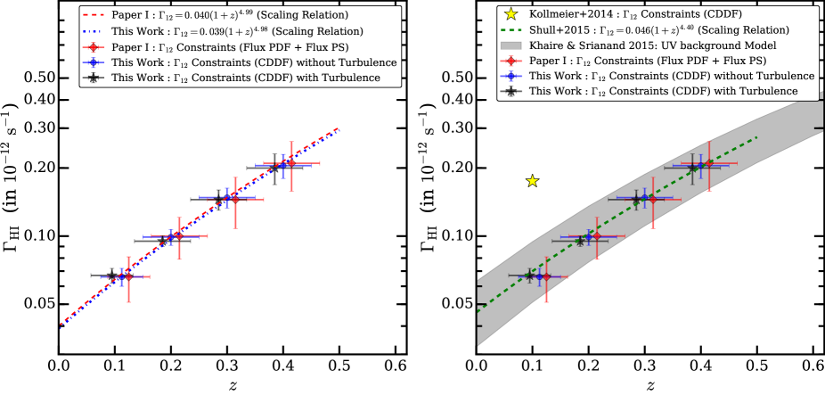
In this section we compare our derived with our previously measured from Paper-I and from the literature at low-. Note previous studies (except Paper-I) do not get through minimization and no errorbars are associated to the measurement. The evolution from this work using CDDF for models with and without turbulence is in good agreement with evolution (using flux PDF and flux PS) from Paper-I. The uncertainty in constraint from Paper-I is larger and more reliable as they also account for other systematic and statistical uncertainties.
Right-hand panel in Fig. 10 shows that our derived () at is lower than from K14 () by factor but is consistent with S15 () within . K14 compared the CDDF in the redshift range with models generated from simulation box at . This could be the possible reason for the discrepancy of constraints obtained in this work and K14. We constrained from CDDF in using models generated from simulation box at ignoring evolution in and large scale structures. The constraint () for this model is higher by factor as compare to constraint from the model at where evolution is accounted for (see Table 1). However, the constraint from this model is in good () agreement with constraint at (, see Table 1) when evolution is accounted for. This is still smaller than what was found by K14. Note that the median redshift of the observed sample is . Thus even if we do not account for evolution, the constraints () are consistent with S15 ( at ) and Paper-I ( at ).
Recently, Gurvich et al. (2016) found that the required to match observed CDDF (from D16) with simulated CDDF is lower than K14 by a factor . They attributed this to the effect of AGN feedback and to the Faucher-Giguère et al. (2009) UVB model included in their simulation. The AGN feedback could be important but is not incorporated in our simulation. However our constraints are in good agreement with those from Gurvich et al. (2016). Note that our constraint at ( , from scaling relation) is consistent within with that from Faucher-Giguère et al. (2009) UVB model ( ). Viel et al. (2016) have provided scaled for different hydrodynamical simulations with and without additional heating that will reproduce the observed CDDF. The direct comparison between our measurements and that of Viel et al. (2016) is difficult as goodness of the CDDF fits and error in are not given in their work. However if we assign 10 percent uncertainty to their measurements, they are very much in agreement with our measurements. Cristiani et al. (2016) found a similar result where their estimated evolution at is in good agreement with evolution from S15 and Paper-I. Cristiani et al. (2016) combined the information from measured QSO contribution to cosmic UVB in the range with QSO luminosity function and estimated the production of ionizing photons from QSOs at various epoch ().
We compare our measured with the UVB model. We find that the UVB generated using updated QSO emissivity (Khaire & Srianand, 2015a) is in very good agreement with our measurements. The gray shaded region in right-hand side of Fig. 10 shows the obtained using this UVB model. This shaded region accounts for two different H i distributions (from Haardt & Madau, 2012; Inoue et al., 2014) and spectral energy distributions of QSOs (Stevans et al., 2014; Lusso et al., 2014) used in the UVB models. measurements can be used to place constraints on escape fraction () of the H i ionizing photons from galaxies (see Inoue et al., 2006; Khaire et al., 2016). Using measured here and uncertainties on it from Paper-I, we find that the is negligible (with star formation history from Khaire & Srianand, 2015b, the limits are 0.8 percent), consistent with measurements of average from low- galaxies (Cowie et al., 2009; Bridge et al., 2010; Siana et al., 2010; Rutkowski et al., 2016). Therefore, low- UVB is predominantly contributed by QSOs.
| Redshift bin | I | II | III | IV |
|---|---|---|---|---|
| Type of simulated spectra | Ly- forest | Ly- forest | Ly- forest | Ly- + Ly- forest1 |
| Best Fit (without turbulence) | 0.066 | 0.104 | 0.137 | 0.199 |
| Statistical uncertainty2 | 0.006 | 0.008 | 0.015 | 0.025 |
| Reduced | 1.49 | 1.39 | 1.24 | 1.35 |
| Best Fit (for Gaussian ) | 0.067 | 0.095 | 0.145 | 0.200 |
| Statistical uncertainty2 | 0.005 | 0.005 | 0.015 | 0.022 |
| Reduced | 1.26 | 1.09 | 1.04 | 1.00 |
-
1
Following Paper-I, simulated Ly- forest at to is contaminated by Ly- forest in the same wavelength range. The Ly- forest is generated from simulation box at .
-
2
The uncertainty in due to uncertainty in thermal history parameters is well within statistical uncertainty.
6 Summary
In this work we constrain the H i photoionization rate and its redshift evolution at from a sample of 82 QSO obtained from Cosmic Origins Spectrograph on board Hubble Space Telescope using H i column density distribution function (CDDF). To explore full range we have developed a code “VoIgt profile Parameter Estimation Routine (viper)” to automatically fit the Ly- absorption lines with Voigt profile. This code is parallel and is written in python. The main results of this work are as follows
-
•
We fitted all the observed Ly- forest spectra using viper and compiled a Ly- line catalog called “viper line catalog”. The fitted parameters such as column density (), line width parameter () and line width distribution from viper line catalog are found to be consistent with those from Danforth et al. (2016). The median parameter from viper ( km s-1) is consistent with that from Danforth et al. (2016, km s-1). Whereas, the median from viper () is in good agreement with that from Danforth et al. (2016, )
-
•
We calculate the appropriate redshift path length and the sensitivity curve from hst-cos data. We calculate the CDDF after accounting for the incompleteness of the sample. Our calculated CDDF in the redshift range () is consistent (KS test -value is 0.83) with that of Danforth et al. (2016) CDDF in the redshift range ().
-
•
We found that the parameters of Voigt profile components from simulations are typically underestimated as compared to observations. This difference can be rectified by including the Gaussian distributed line width parameter ( km s-1and km s-1) at each pixel in the simulation. The resulting line width distribution from simulations matches roughly with observed line width distribution, scatter and lower envelope of the vs distribution. However, the CDDF has little effect of additional ( percent) and the constraints are mildly affected ( percent). However, if we consider additional heating effect for the excess broadening then the obtained will be slightly reduced (roughly scale as ).
-
•
We obtained CDDF at four different bins and matched with simulated CDDF at each mean . This allowed us to measure the in four redshift bins (of ) centered around . We estimated the associated statistical error using statistics. When additional turbulent broadening are not included measured values at the redshift bins are respectively. The corresponding values after inclusion of are . Thus the uncertainties in the velocity broadening seem to have little effect on the derived . Our measured values are in good agreement with Gaikwad et al. (2017) measurement that are obtained with two different statistics namely flux PDF and flux PS. However, the errorbars on measurements of Gaikwad et al. (2017) are more reliable as they account for cosmic variance, continuum fitting uncertainty and cosmological parameter uncertainty in their calculation.
-
•
Our measured is increasing with and follows the relation which is in agreement with Shull et al. (2015). The measured evolution is consistent with Khaire & Srianand (2015a, b) UV background model where it is contributed only by QSOs (i.e., the galaxy contribution is negligible). Inclusion of additional thermal broadening will reduce the value obtained. This will further reduce the galaxy contribution to the at low-.
Acknowledgment
All the computations were performed using the PERSEUS cluster at IUCAA and the HPC cluster at NCRA. We would like to thank Volker Springel, Matteo Viel and Simeon Bird for useful discussion. We also like to thank the referee John Webb and Matthew Bainbridge for improving this work and manuscript.
References
- Akaike (1974) Akaike H., 1974, IEEE Transactions on Automatic Control, 19, 716
- Armstrong (1967) Armstrong B., 1967, Journal of Quantitative Spectroscopy and Radiative Transfer, 7, 61
- Bainbridge & Webb (2016) Bainbridge M. B., Webb J. K., 2016, preprint, (arXiv:1606.07393)
- Becker & Bolton (2013) Becker G. D., Bolton J. S., 2013, MNRAS, 436, 1023
- Becker et al. (2011) Becker G. D., Bolton J. S., Haehnelt M. G., Sargent W. L. W., 2011, MNRAS, 410, 1096
- Bi (1993) Bi H., 1993, ApJ, 405, 479
- Bi & Davidsen (1997) Bi H., Davidsen A. F., 1997, ApJ, 479, 523
- Bi et al. (1992) Bi H. G., Boerner G., Chu Y., 1992, A&A, 266, 1
- Bolton & Haehnelt (2007) Bolton J. S., Haehnelt M. G., 2007, MNRAS, 382, 325
- Bolton et al. (2005) Bolton J. S., Haehnelt M. G., Viel M., Springel V., 2005, MNRAS, 357, 1178
- Bolton et al. (2008) Bolton J. S., Viel M., Kim T.-S., Haehnelt M. G., Carswell R. F., 2008, MNRAS, 386, 1131
- Bridge et al. (2010) Bridge C. R., et al., 2010, ApJ, 720, 465
- Calura et al. (2012) Calura F., Tescari E., D’Odorico V., Viel M., Cristiani S., Kim T.-S., Bolton J. S., 2012, MNRAS, 422, 3019
- Cen et al. (1994) Cen R., Miralda-Escudé J., Ostriker J. P., Rauch M., 1994, ApJ, 437, L9
- Choudhury et al. (2001) Choudhury T. R., Srianand R., Padmanabhan T., 2001, ApJ, 559, 29
- Cooke et al. (1997) Cooke A. J., Espey B., Carswell R. F., 1997, MNRAS, 284, 552
- Cooke et al. (2014) Cooke R. J., Pettini M., Jorgenson R. A., Murphy M. T., Steidel C. C., 2014, ApJ, 781, 31
- Cowie et al. (2009) Cowie L. L., Barger A. J., Trouille L., 2009, ApJ, 692, 1476
- Cristiani et al. (2016) Cristiani S., Serrano L. M., Fontanot F., Vanzella E., Monaco P., 2016, MNRAS, 462, 2478
- Croft et al. (1997) Croft R. A. C., Weinberg D. H., Katz N., Hernquist L., 1997, ApJ, 488, 532
- Croft et al. (1998) Croft R. A. C., Weinberg D. H., Katz N., Hernquist L., 1998, ApJ, 495, 44
- Danforth et al. (2016) Danforth C. W., et al., 2016, ApJ, 817, 111
- Davé & Tripp (2001) Davé R., Tripp T. M., 2001, ApJ, 553, 528
- Davé et al. (2010) Davé R., Oppenheimer B. D., Katz N., Kollmeier J. A., Weinberg D. H., 2010, MNRAS, 408, 2051
- Faucher-Giguère et al. (2008) Faucher-Giguère C.-A., Lidz A., Hernquist L., Zaldarriaga M., 2008, ApJ, 682, L9
- Faucher-Giguère et al. (2009) Faucher-Giguère C.-A., Lidz A., Zaldarriaga M., Hernquist L., 2009, ApJ, 703, 1416
- Fernández-Soto et al. (1996) Fernández-Soto A., Lanzetta K. M., Barcons X., Carswell R. F., Webb J. K., Yahil A., 1996, ApJ, 460, L85
- Gaikwad et al. (2017) Gaikwad P., Khaire V., Choudhury T. R., Srianand R., 2017, MNRAS, 466, 838
- Garzilli et al. (2015) Garzilli A., Theuns T., Schaye J., 2015, MNRAS, 450, 1465
- Gurvich et al. (2016) Gurvich A., Burkhart B., Bird S., 2016, preprint, (arXiv:1608.03293)
- Haardt & Madau (2012) Haardt F., Madau P., 2012, ApJ, 746, 125
- Hernquist et al. (1996) Hernquist L., Katz N., Weinberg D. H., Miralda-Escudé J., 1996, ApJ, 457, L51
- Inoue et al. (2006) Inoue A. K., Iwata I., Deharveng J.-M., 2006, MNRAS, 371, L1
- Inoue et al. (2014) Inoue A. K., Shimizu I., Iwata I., Tanaka M., 2014, MNRAS, 442, 1805
- Jeffreys (1961) Jeffreys H., 1961, Theory of Probability. 3rd edn. Oxford Univ. Press, Oxford
- Keeney et al. (2012) Keeney B. A., Danforth C. W., Stocke J. T., France K., Green J. C., 2012, PASP, 124, 830
- Khaire & Srianand (2015a) Khaire V., Srianand R., 2015a, MNRAS, 451, L30
- Khaire & Srianand (2015b) Khaire V., Srianand R., 2015b, ApJ, 805, 33
- Khaire et al. (2016) Khaire V., Srianand R., Choudhury T. R., Gaikwad P., 2016, MNRAS, 457, 4051
- King et al. (2011) King J. A., Murphy M. T., Ubachs W., Webb J. K., 2011, MNRAS, 417, 3010
- Kollmeier et al. (2014) Kollmeier J. A., et al., 2014, ApJ, 789, L32
- Liddle (2007) Liddle A. R., 2007, MNRAS, 377, L74
- Lidz et al. (2010) Lidz A., Faucher-Giguère C.-A., Dall’Aglio A., McQuinn M., Fechner C., Zaldarriaga M., Hernquist L., Dutta S., 2010, ApJ, 718, 199
- Lusso et al. (2014) Lusso E., et al., 2014, ApJ, 784, 176
- McDonald et al. (2000) McDonald P., Miralda-Escudé J., Rauch M., Sargent W. L. W., Barlow T. A., Cen R., Ostriker J. P., 2000, ApJ, 543, 1
- McDonald et al. (2001) McDonald P., Miralda-Escudé J., Rauch M., Sargent W. L. W., Barlow T. A., Cen R., 2001, ApJ, 562, 52
- McDonald et al. (2005) McDonald P., et al., 2005, ApJ, 635, 761
- McQuinn et al. (2011) McQuinn M., Hernquist L., Lidz A., Zaldarriaga M., 2011, MNRAS, 415, 977
- Meiksin & White (2004) Meiksin A., White M., 2004, MNRAS, 350, 1107
- Miralda-Escudé et al. (1996) Miralda-Escudé J., Cen R., Ostriker J. P., Rauch M., 1996, ApJ, 471, 582
- Muzahid et al. (2012) Muzahid S., Srianand R., Bergeron J., Petitjean P., 2012, MNRAS, 421, 446
- Oppenheimer & Davé (2009) Oppenheimer B. D., Davé R., 2009, MNRAS, 395, 1875
- Padmanabhan et al. (2015) Padmanabhan H., Srianand R., Choudhury T. R., 2015, MNRAS, 450, L29
- Penton et al. (2000) Penton S. V., Shull J. M., Stocke J. T., 2000, ApJ, 544, 150
- Phillips et al. (2001) Phillips J., Weinberg D. H., Croft R. A. C., Hernquist L., Katz N., Pettini M., 2001, ApJ, 560, 15
- Planck Collaboration et al. (2015) Planck Collaboration et al., 2015, preprint, (arXiv:1502.01589)
- Pontzen et al. (2014) Pontzen A., Bird S., Peiris H., Verde L., 2014, ApJ, 792, L34
- Press et al. (1992) Press W. H., Teukolsky S. A., Vetterling W. T., Flannery B. P., 1992, Numerical recipes in FORTRAN. The art of scientific computing
- Rauch et al. (1997) Rauch M., et al., 1997, ApJ, 489, 7
- Rollinde et al. (2013) Rollinde E., Theuns T., Schaye J., Pâris I., Petitjean P., 2013, MNRAS, 428, 540
- Rutkowski et al. (2016) Rutkowski M. J., et al., 2016, ApJ, 819, 81
- Schaye (2001) Schaye J., 2001, ApJ, 559, 507
- Schaye et al. (1999) Schaye J., Theuns T., Leonard A., Efstathiou G., 1999, MNRAS, 310, 57
- Schaye et al. (2000) Schaye J., Theuns T., Rauch M., Efstathiou G., Sargent W. L. W., 2000, MNRAS, 318, 817
- Schneider et al. (1993) Schneider D. P., et al., 1993, ApJS, 87, 45
- Scoccimarro et al. (2012) Scoccimarro R., Hui L., Manera M., Chan K. C., 2012, Phys. Rev. D, 85, 083002
- Seljak et al. (2006) Seljak U., Slosar A., McDonald P., 2006, J. Cosmology Astropart. Phys., 10, 014
- Shull et al. (2012) Shull J. M., Smith B. D., Danforth C. W., 2012, ApJ, 759, 23
- Shull et al. (2015) Shull J. M., Moloney J., Danforth C. W., Tilton E. M., 2015, ApJ, 811, 3
- Siana et al. (2010) Siana B., et al., 2010, ApJ, 723, 241
- Smith et al. (2011) Smith B. D., Hallman E. J., Shull J. M., O’Shea B. W., 2011, ApJ, 731, 6
- Springel (2005) Springel V., 2005, MNRAS, 364, 1105
- Springel & Hernquist (2002) Springel V., Hernquist L., 2002, MNRAS, 333, 649
- Stevans et al. (2014) Stevans M. L., Shull J. M., Danforth C. W., Tilton E. M., 2014, ApJ, 794, 75
- Storrie-Lombardi et al. (1996) Storrie-Lombardi L. J., McMahon R. G., Irwin M. J., 1996, MNRAS, 283, L79
- Tegmark et al. (2004) Tegmark M., et al., 2004, ApJ, 606, 702
- Tepper-García et al. (2012) Tepper-García T., Richter P., Schaye J., Booth C. M., Dalla Vecchia C., Theuns T., 2012, MNRAS, 425, 1640
- Tripp et al. (2008) Tripp T. M., Sembach K. R., Bowen D. V., Savage B. D., Jenkins E. B., Lehner N., Richter P., 2008, ApJS, 177, 39
- Viel & Haehnelt (2006) Viel M., Haehnelt M. G., 2006, MNRAS, 365, 231
- Viel et al. (2004a) Viel M., Haehnelt M. G., Springel V., 2004a, MNRAS, 354, 684
- Viel et al. (2004b) Viel M., Weller J., Haehnelt M. G., 2004b, MNRAS, 355, L23
- Viel et al. (2006) Viel M., Haehnelt M. G., Lewis A., 2006, MNRAS, 370, L51
- Viel et al. (2009) Viel M., Bolton J. S., Haehnelt M. G., 2009, MNRAS, 399, L39
- Viel et al. (2016) Viel M., Haehnelt M. G., Bolton J. S., Kim T.-S., Puchwein E., Nasir F., Wakker B. P., 2016, preprint, (arXiv:1610.02046)
- Webb & Carswell (1991) Webb J. K., Carswell R. F., 1991, in Shaver P. A., Wampler E. J., Wolfe A. M., eds, Quasar Absorption Lines. p. 3
- Zaldarriaga et al. (2001) Zaldarriaga M., Hui L., Tegmark M., 2001, ApJ, 557, 519
- Zhang et al. (1995) Zhang Y., Anninos P., Norman M. L., 1995, ApJ, 453, L57
Appendix
We formed a line catalog by fitting the observed spectra using viper. Table 2 shows few fitted parameters from the viper line catalog for spectra towards QSO 1ES1553+113. The first, second, third, fourth, fifth and sixth column shows fitted wavelength ( in ), error in wavelength ( in ), log of column density ( in cm-2), error in log of column density ( d in cm-2), parameter (in km s-1) and error in parameter ( in km s-1) respectively. The full viper line catalog is available online in ASCII format with this paper.
| d | d | ||||
|---|---|---|---|---|---|
| () | () | ( cm-2) | ( cm-2) | ( km s-1) | ( km s-1) |
| 1330.827 | 0.003 | 13.68 | 0.01 | 32.06 | 1.08 |
| 1339.936 | 0.002 | 14.23 | 0.01 | 38.09 | 0.80 |
| 1361.466 | 0.019 | 12.84 | 0.06 | 34.10 | 7.00 |
| 1361.922 | 0.013 | 12.94 | 0.05 | 28.91 | 4.99 |
| 1365.408 | 0.018 | 13.04 | 0.04 | 48.75 | 5.57 |