Revealing a spiral-shaped molecular cloud in our galaxy – Cloud fragmentation under rotation and gravity

The dynamical processes that control star formation in molecular clouds are not well understood, and in particular, it is unclear if rotation plays a major role in cloud evolution. We investigate the importance of rotation in cloud evolution by studying the kinematic structure of a spiral-shaped Galactic molecular cloud G052.24$+$00.74. The cloud belongs to a large filament, and is stretching over $\sim 100\;\rm pc$ above the Galactic disk midplane. The spiral-shaped morphology of the cloud suggests that the cloud is rotating. We have analysed the kinematic structure of the cloud, and study the fragmentation and star formation. We find that the cloud exhibits a regular velocity pattern along west-east direction – a velocity shift of $\sim 10\;\rm km\;s^{-1}$ at a scale of $\sim 30$ pc. The kinematic structure of the cloud can be reasonably explained by a model that assumes rotational support. Similarly to our Galaxy, the cloud rotates with a prograde motion. We use the formalism of Toomre (1964) to study the cloud’s stability, and find that it is unstable and should fragment. The separation of clumps can be consistently reproduced assuming gravitational instability, suggesting that fragmentation is determined by the interplay between rotation and gravity. Star formation occurs in massive, gravitational bound clumps. Our analysis provides a first example in which the fragmentation of a cloud is regulated by the interplay between rotation and gravity.

1 Introduction

Star formation takes place in the dense and shielded parts of the molecular interstellar medium. An increasingly dynamical picture of cloud evolution has been revealed by recent observations and simulations (Dobbs et al. 2014; Heyer & Dame 2015, and references therein). Star formation may be determined by a combination of turbulence (Mac Low & Klessen 2004; Hennebelle & Falgarone 2012), gravity (Heyer et al. 2009; Ballesteros-Paredes et al. 2011, 2012), magnetic field (Li et al. 2014) and ionisation radiation (Whitworth et al. 1994; Dale et al. 2009).

The hierarchical structures of molecular clouds are produced by a series of fragmentation processes. In the theory of turbulence-regulated star formation (Ballesteros-Paredes et al. 1999; Padoan & Nordlund 1999; Mac Low & Klessen 2004; Krumholz & McKee 2005), supersonic turbulence creates a set of density fluctuations, and it is the high-density parts that undergo gravitational collapse. It has also been alternatively proposed that the evolution of molecular clouds is governed by gravity, and gravitational collapse creates a hierarchy of structures which then form stars (Hoyle 1953; Larson 1973; Zinnecker 1984; Heitsch & Hartmann 2008; Ballesteros-Paredes et al. 2011). It is unclear what dominates the evolution of molecular clouds.

In recent years, the importance of environment on cloud evolution has been addressed. It is now relatively well-recognised that molecular clouds are not isolated objects. They can belong to large-scale structures (Ragan et al. 2014; Wang et al. 2015; Zucker et al. 2015; Li et al. 2016; Abreu-Vicente et al. 2016; Li et al. 2013), suggesting a connection between Galactic shear and cloud evolution. A connection between cloud evolution and large-scale magnetic field has also been suggested (Li et al. 2015). Moreover, cloud evolution can be significantly influenced by stellar feedback (Elmegreen & Lada 1977; Whitworth et al. 1994; Whitworth & Francis 2002). All these effects have been proven to be important at least in some cases. Nevertheless, the role of angular momentum in molecular clouds is still unclear.

In this work, we present a study of a spiral-shaped molecular cloud G052.24$+$00.74. The cloud is identified from the Galactic Ring Survey (Jackson et al. 2006). It belongs to a large ($\sim$ 500 pc) gas filament (filamentary gas wisp) discussed in an earlier work (Li et al. 2013). The molecular gas of the cloud is distributed in spiral-arm-like features, and we have named it “Spiral Cloud”. The whole cloud exhibits a regular velocity pattern and clear signs of fragmentation on the “spiral arm” part of the cloud. A star cluster has already formed in one of the clumps. In this paper we focus on the global kinematic structure of the cloud, and addresses its connection with the ongoing star formation activities.

2 Archival data

We used ¹³CO(1-0) molecular line data ($\nu_{0}=110.2\rm\;GHz$) from the Galactic Ring Survey (Jackson et al. 2006), which is a survey of the Milky Way disk with the SEQUOIA multipixel array on the Five College Radio Astronomy Observatory 14 m telescope, and covers a longitude range of $18^{\circ}<l<55.7^{\circ}$ and a latitude range of $|b|<1^{\circ}$ with a spatial resolution of $46\arcsec$. The beam efficiency is $\eta_{\rm mb}$ = 0.48 (Ridge et al. 2006). At a distance of 9.8 kpc (Li et al. 2013), the spatial resolution is around 2.2 pc. The velocity resolution is $0.22\;\rm km/s$. For our region, the rms sensitivity is $\sigma(T_{\rm A^{*}})\approx 0.24\,\rm K$. These observations are velocity-resolved which allowed us to trace and analyse the cloud’s kinematic structure in detail.

We have made use of 3.6 $\mu$m and 8 $\mu$m data from the GLIMPSE project (Benjamin et al. 2003), which is a fully sampled, confusion-limited, four-band near-to-mid infrared survey of the inner Galactic disk. We use 24 $\mu$m data from the MIPSGAL project (Carey et al. 2009), which is a survey of the Galactic disk with the MIPS instrument on Spitzer at 24 $\mu$m and 70 $\mu$m. The 3.6 $\mu$m emission is sensitive to the presence of YSOs, and the 8 $\mu$m emission typically traces polycyclic aromatic hydrocarbon (PAHs). Star formation can be traced by the 24 $\mu$m emission, which originates from the dust heated by newly-born stars.

3 Results

3.1 Multi-scale structure

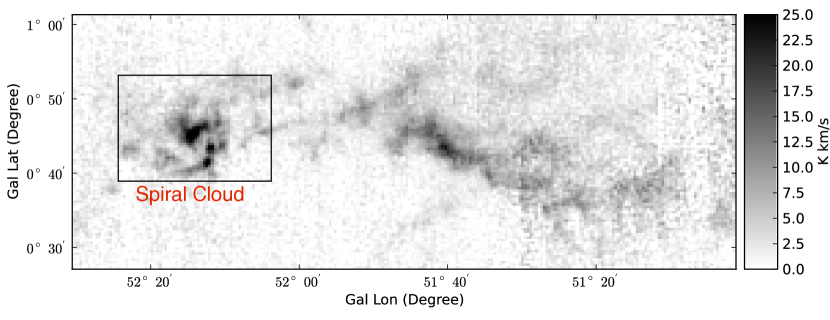
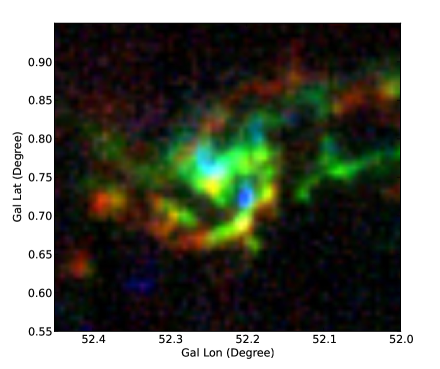
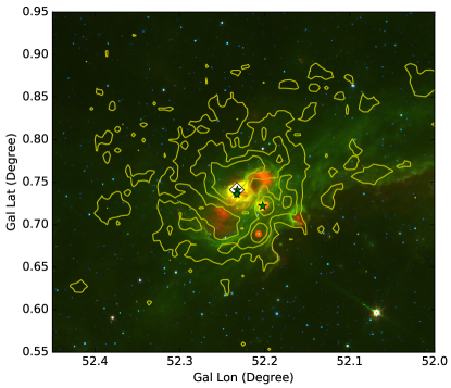
Figure 1: Upper panel: ¹³CO(1-0) emission integrated from -4.5 to 15.0 $\rm km\;s^{-1}$ from the GRS survey (Jackson et al. 2006). The cloud G052.24+00.74 is on the left side. This cloud is connected with the neighbouring cloud G051.69+00.74 by some filamentary gas wisps. Channel maps of the region can be found in Appendix A. Lower left panel: Composite three-color image of the ¹³CO(1-0) emission from the Spiral Cloud G052.24+00.74. Red: $6.52<\textit{v}_{\rm lsr}<15.0\;\rm km\;s^{-1}$ Green: $3.12<\textit{v}_{\rm lsr}<6.10\;\rm km\;s^{-1}$ Blue: $-4.53<\textit{v}_{\rm lsr}<2.7\;\rm km\;s^{-1}$. The velocity centroid map and velocity FWHM map can be found in Appendix D. Lower right panel: Spitzer GLIMPSE (Benjamin et al. 2003) and MPISGAL three-color image of the Spiral Cloud G052.24+00.74. Red: 24 $\mu$m, Green: 8 $\mu$m, Red: 3.6 $\mu$m. Overlaid contours are the velocity-integrated ¹³CO(1-0) emission (integrated from $-4.5{\rm km/s}<\textit{v}_{\rm lsr}<11.5\;\rm km/s$). Contours correspond to 5.1, 10.2, 15.3 $\rm K\;km\;s^{-1}$. The white diamond at the centre stands for a star cluster discovered in the GLIMPSE survey (Mercer et al. 2005), and the green stars stand for H ii   regions collected from the literature (Lockman 1989; Urquhart et al. 2009).

From the ¹³CO data of the GRS survey (Fig. 1) we found that the cloud belongs to a larger system of two clouds (the Spiral Cloud, G025.24$+$00.74 and G051.69$+$00.74). This double cloud system has a total mass of $1.2\times 10^{5}\;M_{\odot}$ (Roman-Duval et al. 2010) and a total physical extent of $\sim 140\;\rm pc$. Wisps of molecular gas connect the cloud with another cloud at $l\sim 51^{\circ}$ (G051.69+00.74). The lower boundary of the two clouds is arc-like, and is associated with the G52L nebula in Bania et al. (2012).

This large double cloud system stretches to a $\sim 500\;\rm pc$ filamentary gas wisp (Li et al. 2013). Recently, such filamentary structures have been found to be relatively common throughout the Galaxy (Ragan et al. 2014; Wang et al. 2015; Zucker et al. 2015; Li et al. 2016; Abreu-Vicente et al. 2016) and are predicted by theory and simulations (Smith et al. 2014; Dobbs 2015; Pringle et al. 2001).

3.2 Structure of the cloud

The whole Spiral Cloud has a mass of $2.72\times 10^{4}M_{\odot}$ and a radius of $\sim 12\;\rm pc$ (Roman-Duval et al. 2010). It has a centrally-condensed morphology, and exhibits a regular velocity pattern (Fig. 1, 14) where the south-eastern part of the cloud is red-shifted and the north-western part of the cloud is blue-shifted. The spiral-shaped structure lead us to assume that the velocity difference originates from rotation. The inferred cloud rotation is similar to the Milky Way rotation, and the projected angle between the cloud rotational axis and the rotation axis of the Galactic disk is estimated to be 22.5^∘ (measured directly from the map). The rotation is also visible in channel maps (Fig. 9). Velocity centroid map and velocity FWHM map can be found in Appendix D.

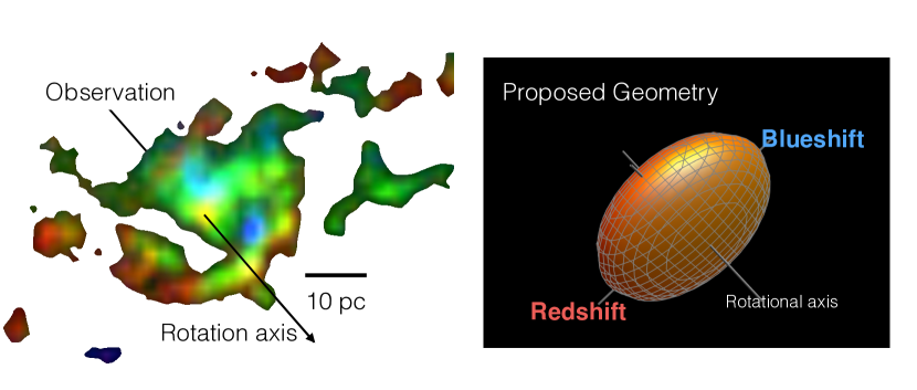
Figure 2: An illustration of the geometry of the Spiral Cloud. The left panel is a 3-colour rendering of the spiral cloud. Red colour stand for redshifted gas, and blue colour stand for blueshifted gas. On top of the image, we overlay the suggested rotational axis. In the right panel, we present a 3D ellipsoid, with two longer axes and one shorter axis. The orientation mimic the suggested orientation of the spiral cloud. The ellipsoid (representing the Spiral Cloud) is rotating with respect to its shorter axis, which we have indicated in the plot. The western side of the Spiral Cloud is rotating toward the observer. The angle between the rotational axis of the Spiral Cloud and the rotational axis of the Milky Way disk is estimated to be $22.5^{\circ}$, and the cloud inclination is estimated to be $45^{\circ}$.

Because of the observed rotational pattern, we assume that in 3D the cloud can be approximated as an ellipsoid characterised by two longer axis and one shorter axis, and is rotating with respect to its shorter axis. A prior, the cloud’s inclination is unknown , and from the map we estimate an inclination of 45^∘. Because of projection, one can not readily tell which part of the cloud is closer to us in 3D. However, we can still infer the 3D geometry by assuming that the spiral arms are trailing, and thus we infer the orientation of the cloud as illustrated in Fig. 2.

To better analyse the cloud structure from the centre to the outside, we divided the ¹³CO(1-0) map into rings. Ideally, each of the ring corresponds to a circle were the cloud is viewed face-on. We measured the longer and shorter axes manually from the map. Based on this, we divided the cloud into different rings. The semi-major axes of the rings (which correspond to the radii of the circles in 3D when de-projected) are called cloud radii. The widths of the rings were chosen to be 2.7 pc, which is larger and still comparable to the resolution derived from the beam size (2.2 pc). The structure of the individual rings can be found in Appendix C. The velocity structure of the cloud can be well seen in each ring.

For each ring, we measured the mean column density. The velocity range was chosen to be $-4.5{\rm km/s}<\textit{v}_{\rm lsr}<11.5\;\rm km/s$ to cover the whole cloud. To focus on the spiral structure, we only analysed regions that have $\int T_{\rm A*}\rm{dv}\geq 5.1\rm K\;km\;s^{-1}$. This corresponds to 3.5 times the rms noise level. The corresponding region is indicated in Fig. 10.

We estimated the $\rm H_{2}$ column density using ${N}_{\rm H_{2}}=5\times 10^{20}\;{\rm T}_{\rm mb}\,{\rm d}{\rm v}/(\rm K\;km\;s^{-1})$ (Simon et al. 2001). ${\rm T}_{\rm mb}={\rm T}_{\rm A*}/\eta_{\rm mb}$, where ${\rm T}_{\rm A*}$ is the antenna temperature and $\eta_{\rm mb}$ is the beam efficiency, $\rm v$ is the velocity. This conversion has been derived assuming an excitation temperature ${T}_{\rm ex}=10\rm K$, and a ¹³CO abundance ${\rm R}(^{13}{\rm CO/H_{2}})=1.7\times 10^{-6}$. Fig. 3 shows the mean surface density as a function of the sizes of the rings (which we named Cloud Radius $r_{\rm cloud}$). From Fig. 3, we found that mean column density measured in H₂ can be expressed as a function of cloud radius $r_{\rm cloud}$:

$$N_{\rm H_{2}}=1.5\times 10^{22}{\rm cm^{-2}}\times\big{(}\frac{r_{\rm cloud}}{\rm 5\;pc}\big{)}^{-1}\;.$$ (1)

The surface density of the cloud can be estimated as $\Sigma=N_{\rm H_{2}}\times m_{\rm H_{2}}\times 1.36$ where $m_{\rm H_{2}}$ is the mass of $\rm H_{2}$ and $1.36$ is the correction for Helium and other heavy elements. At the outer regions, Eq. 1 captures the structure of the cloud quite well, but at the inner $\sim 3$ pc region, there are some noticeable differences between the column density in the analytical model and the observational data. However, this discrepancy is not severe since this is also the region where the ¹³CO is likely to be optically thick and the observations are underestimating the column density.

Assuming that the gas in the cloud stays in a flattened disk, by taking advantage of the the fact that the column density scales as $r_{\rm cloud}^{-1}$, one can analytically evaluate the expected rotation profile following Mestel (1963). Disks that share this kind of density profiles are called “Mestel disks”. The rotation velocity profiles can be determined from the balance between centrifugal force and gravitational force, they are flat, characterised by constant circular velocities. In the case of our disk, the model is accurate only at $r_{\rm cloud}\gtrsim 5\;\rm pc$ where the model does capture the density structure to a reasonable accuracy. The theoretical circular velocity can be computed as

$${\rm v}_{\rm circ}^{\rm model}=2\;\pi\;G\;\Sigma_{0}\;r_{0}=6.6\;\rm km/s,$$ (2)

where $\Sigma_{0}r_{0}$ can be found in Eq. 1, $r_{0}=5\;\rm pc$ and $\Sigma_{0}$ can be evaluated from Eq. 1. Assuming that the cloud is rotationally supported, the absolute velocity difference between the left and right side of the disc is thus of $2\rm\;v_{\rm cir}$ (i.e. 13.2 $\rm km/s$).

Assuming an inclination of $45^{\circ}$, the predicted velocity shift of either side of the disk is 4.68 $\rm km/s$ with respect to the systemic velocity. This is the theoretically-expected velocity shift if we assume that the cloud is gravitationally bound and has a disk-like geometry.

In Appendix C we compare the velocity structure of the cloud with the expected velocity structure derived from the Mestel (1963) model. In general, the agreement is better at $r_{\rm cloud}\gtrsim 15\;\rm pc$. Inside the inner 15 pc, the velocity difference is not always obvious. However, in this region, the model is not so accurate because of the deviation of the real density profile from the density profile of the Mestel (1963) model, and the data are not accurate either, because of the observed line widths are typically large (around a few $\rm km/s$).

The agreement between the model and the data leads us to conclude that the cloud is probably rotationally-supported. We note, however, that there are still structures that do not follow this regular rotation pattern. A few explanations are possible: first, the cloud is already fragmented, and for each ring, only a small portion is sampled by the molecular gas. Thus this incomplete sampling introduces some irregularities to our data. Second, for each line of sight, a typical line width of $\sim 1\;\rm km/s$ is common (see e.g. Table 1). Third, the cloud is already fragmented, and the very process of gravitational instability can introduce significant deviations from regular circular rotation. The gas motion would also be influenced by the expansion of the embedded H_II regions. These observational and theoretical uncertainties can potentially account for the observed velocity irregularities.

3.3 Fragmentation

We used the Dendrogram program (Rosolowsky et al. 2008; Goodman et al. 2009) to quantify the clumpy structure of the cloud. The Dendrograms are representations of how the isosurfaces in a 3-D PPV data cube nest inside one another. The “Leaves” of a Dendrogram correspond to the regions that have emission enhancements in the 3-D PPV data cube, and they correspond to the “clumps” found by the well-known clumpfind algorithm (Williams et al. 1994). One advantage of using Dendrogram is that its results are less dependent on technical parameters (for instance, the brightness temperature difference between contours). In this work, the term cloud is used to refer to the whole cloud G052.24$+$00.74, and the term clump is used to refer to the sub-structures of the cloud identified by the Dendrogram algorithm.

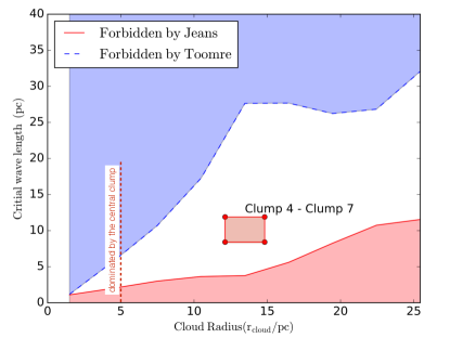
Figure 6: Physical scales involved in the fragmentation process. The $x$-axis is the cloud radius, and the $y$-axis denotes the critical length scales involved in the fragmentation process. The blue dashed line stands for the Toomre length $l_{\rm Toomre}=2\pi G\Sigma/\kappa^{2}$. In the blue shaded region fragmentation is suppressed due to shear. The red solid line stands for the Jeans length $l_{\rm Jeans}=2\sigma_{\rm v}^{2}/G\Sigma$ where we have chosen $\sigma_{v}=1\;\rm km/s$. In red shaded region fragmentation is suppressed due to thermal-turbulent support. The clumps 4 and 7 form a pair at a cloud radius of 13.5 pc, and they are separated by 10 pc. It is indicated in this diagram as the red square, where the size of the square represents the estimated uncertainty. Since we did not de-project the clump separation into 3D, and the cloud is inclined with an angle of $45^{\circ}$, we estimate an uncertainty of $\sqrt{2}$ (see text for details). The central 5 pc is dominated by the central clump (measured from from Fig. 10), where we do not expect our analysis to apply. This is indicated by the vertical red dashed line.

In this work, we smoothed the data in the velocity direction. The smoothed data cube has a velocity resolution of 0.4 km/s and a rms noise level of $0.17$ K. Then we identify clumps from the data using the Dendrogram program. The program requires three inputs, the minimum value to consider in the dataset (min_value), and minimum difference for a structure to be considered as independent (min_delta), as well as the minimum number of pixels in a given structure (min_npix). We use min_value = 0.67 K, min_delta = 0.33 K and min_npix = 16. This choice of the parameters is relatively conservative, which ensures that only highly significant structures are considered independent. A change of these thresholds to lower values produces a larger number of smaller clumps, but the significant (e.g. these marked red in Fig. 6) structures remain unchanged.

One should also note that the velocity dispersions of the extracted structures are dependent on the choice of the parameters. Structures identified with a relatively high threshold are more compact in 3D PPV space, and thus have smaller velocity dispersions. This may be part of the reason why the total velocity dispersions (e.g. as in Fig. 14) estimated on lines of sights are larger than the velocity dispersion of the clumps.

In Figure 5 we plot the leaves of the Dendrogram. IDs of the leaves are also plotted. A detailed catalogue can be found in Appendix B.

Toomre (1964) developed a theory for the stability of a disk of stars. The formalism is general and has been applied to various systems that are rotationally supported, such as disk galaxies and protostellar disks. In this formalism, the stability of a disk is characterised by the Toomre Q parameter

$$Q=\frac{\sigma_{\rm v}\kappa}{\pi G\Sigma}\;,$$ (3)

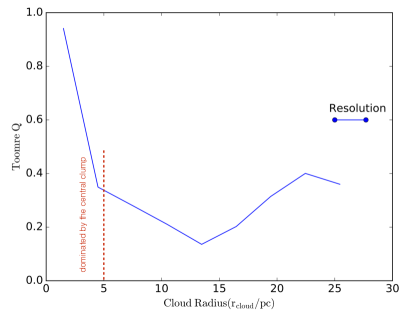
Figure 4: Toomre Q parameter as a function of cloud radius ($r_{\rm cloud}$). The Toomre Q is defined as $Q=\sigma_{\rm v}\kappa/\pi G\Sigma$ where $\sigma_{\rm v}=1\;\rm km/s$, $\Sigma$ is the ring-averaged column density and $\kappa$ is the epicyclic frequency. The resolution of the plot is 2.7 pc (limited by the size of the rings). It is indicated as the blue horizontal bar. The central 5 pc is dominated by the central clump. This is indicated by the vertical red dashed line.

where $\kappa$ is the epicyclic frequency, $\sigma_{\rm v}$ represents “internal” supports such as thermal support and turbulence, and $\Sigma$ is the surface density. If $Q>1$ the disk is stable, and if $Q<1$ the disk is unstable against perturbations and would fragment. We choose $\sigma_{\rm v}=1\;\rm km/s$, which is the typical velocity dispersion to expect for clumps (Wienen et al. 2015) . In Fig. 4 plot the Toomre Q as a function of disk radius. Except the central region, the disk is unstable with $Q<1$. This is consistent with the fact that the disk fragments into clumps due to gravitational instability.

In the formalism of Toomre (1964) (see also Binney & Tremaine 2008; Elmegreen & Elmegreen 1983), the fragmentation is determined by two length scales: the Toomre length and the Jeans length. The Toomre length is defined as

$$l_{\rm Toomre}=\frac{2\pi G\Sigma}{\kappa^{2}}\;.$$ (4)

For disks with flat rotational profiles, $\kappa=\sqrt{2}\Omega$ where $\Omega$ is the angular velocity, and $\Omega=v_{\rm circ}/r=6.6\;\rm km/s/r_{\rm cloud}$ in our case. This sets an upper limit to the fragmentation length scale, and the growth of perturbations with $l>l_{\rm Toomre}$ are suppressed due to shear. The Jeans length is defined as

$$l_{\rm Jeans}=\frac{2\sigma_{\rm v}^{2}}{G\Sigma}\;,$$ (5)

where $\sigma_{v}$ is the velocity dispersion, and it includes thermal and non-thermal (e.g. turbulent) contributions. The Jeans length is a lower limit to the fragmentation length, and growth of perturbations with $l<l_{\rm Jeans}$ are suppressed due to thermal and non-thermal (e.g. turbulent) supports. Only perturbations with $l_{\rm Jeans}<l<l_{\rm Toomre}$ can be amplified.

The fragmentation length scale can be probed by studying the separations of the neighbouring clumps. In Fig. 6 we plot these two length scales as a function of cloud radius (defined in Sect. 3.2). From the cloud, we identify a pair of clumps (4 – 7 , see Fig. 5). Excluding the clump at the very centre, this is the only pair of clumps that are significant on the ATLASGAL (Schuller et al. 2009) tile and thus covered in subsequent studies (Wienen et al. 2015). The clump pair 4–7 share a cloud radius of 14 parsec and are separated by $\sim 10$ parsec. They are well separated and both exhibit signs of star formation. Since we did not deproject the separation into 3D, we estimate an uncertainty of $\sqrt{2}$ of the clump separation estimate (because the cloud inclination is $45^{\circ}$). In Fig. 6, this pair occupies a position where the growth of perturbations is allowed. The predicted length scale of the fragmentation process using the formalism of Toomre (1964) matches well with the observed clump separation. Interestingly, this pair also stays at a radius where the fragmentation is most likely to occur (measured by the difference between $l_{\rm Jeans}$ and $l_{\rm Toomre}$). This supports our hypothesis that the Spiral Cloud fragments due to gravitational instability.

3.4 Star formation in the clumps

To further study the fragmentation process, we divide the leaves (clumps) into different groups. First, we make a distinction between the clumps inside the spiral arm and the clumps outside the spiral arm. Second, since three of the clumps (clump 2, 4 and 7) show evidences of star formation (inside clump 2, a star cluster has already formed, and massive stars inside this star cluster are probably triggering the formation of a next generation of stars. A bubble is found in clump 7. RMS YSOs are found in clump 4 (Thompson et al. 2012)), we separate them from the rest of the clumps. Finally, we have three groups of clumps. The first group include the clumps that exhibit obvious star formation activities (clump 2, 4 and 7), the second group include the other clumps that are inside the spiral arm, and the third group consists of the rest of the clumps.

We analyse the physical properties of the three different groups of clumps. In deriving the properties, we use the same formalism as used in Goodman et al. (2009). The detailed properties of the clumps can be found in Appendix B. In Fig. 7, we plot $\sigma_{\rm v}^{2}/R$ versus $\Sigma$ for all the clumps (Simon et al. 2001, where $\Sigma\equiv M/\pi R^{2}$). Lines of different virial parameters are derived from (Bertoldi & McKee 1992)

$$\alpha_{\rm vir}=\frac{5\sigma_{\rm v}^{2}R}{GM}\;,$$ (6)

where $\alpha_{\rm vir}$ is the viral parameter, $\sigma_{\rm v}$ is the velocity dispersion of the clumps, $R$ is the radii of the clumps, G is gravitational constant, and $M$ is the mass clump. The clumps that belong to the spiral arm are close to gravitationally bound ($0.5<\alpha_{\rm vir}<1$), while the other clumps are not. Interestingly, all the three clumps that show star formation activities are gravitationally bound.

The correspondence of a small viral parameter and active star formation leads us to suggest that the star formation inside the clumps is controlled largely by self-gravity. Another way to look at the problem is to consider the free-fall timescale. This is a characteristic timescale that governs the gravitational collapse. It is defined as $t_{\rm ff}\sim(G\rho)^{-1/2}$, $\rho\equiv M/R^{3}$. In Figure 8 we plot the masses of the clumps against the radii of the clumps. Lines that correspond to different free-fall timescales $t_{\rm ff}$ are added. The clumps that belong to the spiral arm have significantly shorter free-fall timescales, and the three clumps that are forming stars have not only short free-fall timescales but also higher masses.

A star cluster has formed at the centre of clump 2 (Mercer et al. 2005). This clump is distinguished in two ways. First, it is the clump that resides right at the centre of the spiral structure. Second, compared to all the other clumps, it has the smallest viral parameter and the shortest free-fall timescale. The connection between star formation and indicators of the importance of self-gravity suggests that gravity is playing a determining role in the evolution of the clumps. Kauffmann et al. (2010) derived an empirical threshold ${\rm M}=870\,{\rm M}_{\odot}({\rm r/pc)^{1.33}}$ for the formation of massive stars in the mass-size plane, e.g. clumps that are above this line are active in massive star formation. The results have been confirmed by studies of larger samples, e.g. ATLASGAL clumps (Urquhart et al. 2013). This threshold is also indicated in Fig. 8. Only clumps 2, 4 and 7 host H ii   regions , and clumps 2 and 4 are above this threshold. However, we note that the result is true for these clump-like objects only in a statistical sense.

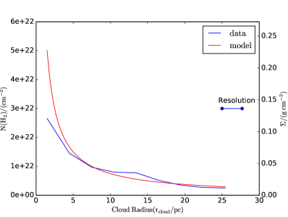
Figure 3: Column density structure of the Spiral Cloud. The figure presents ring-averaged column density as a function of cloud radius. The blue line stands for the data and the red line stands for the analytical model (Eq. 1). The telescope resolution is $\sim 2.2\;\rm pc$ at a distance of $9.8\;\rm kpc$. The resolution of the plot (2.7 pc, limited by the widths of the rings) is indicated as the blue horizontal bar. See Sect. 3.2 for details.

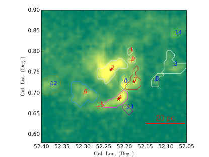
Figure 5: Clumps (leaves) identified by the Dendrogram method. Here we use different colours to indicate different leaves for clarity. Each leaf has a unique ID. We divide the leaves into three groups, one group contains clumps that belong to the “spiral arm” of the cloud (red numbers), and the other group contain clumps that are outside the “spiral arm” (blue numbers). The third group contains clumps 2, 4 and 7, which exhibit clear evidences of ongoing star formation (red stars).

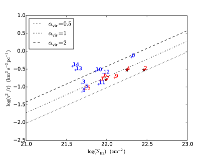
Figure 7: Ratio of $\sigma_{v}^{2}/R$ as a function of clump column density $N_{\rm H_{\rm 2}}$. We divide the leaves into three groups, one group contains the clumps that belong to the spiral arm of the cloud (red crosses), and the other group contains clumps that are outside the spiral arm (blue crosses). The third group contains clump 2,4 and 7, which exhibit clear evidences of ongoing star formation (red stars with numbers). IDs of the clumps are indicated Lines of different virial parameters $\alpha_{\rm vir}=5\sigma_{\rm v}^{2}R/G\Sigma$ are included.

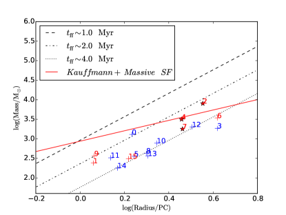
Figure 8: Clump mass versus clump radius for all the clumps. We divide the clumps into three groups, one group contains the clumps that belong to the spiral arm of the cloud (red crosses), and the other group contain the clouds that are outside the “spiral arm” (blue crosses). The third group contains clumps 2, 4 and 7, which exhibit clear evidences of ongoing star formation (red stars with numbers). IDs of the clumps are indicated. Lines of different free-fall time $t_{\rm ff}\sim\rho^{-1/2}$ are included. The red solid line corresponds to the threshold of massive star formation ${\rm M}=870\,{\rm M}_{\odot}({\rm r/pc)^{1.33}}$ derived in Kauffmann et al. (2010).

4 Rotating molecular clouds in observations and simulations

How do molecular clouds evolve? It is widely recognised that cloud evolution is governed by the combined effects of (ordered or disordered) kinematic motion, turbulence, gravity and magnetic field. However, the relative importance of these factors is not known. The importance of rotation in cloud evolution has long been recognised (Phillips 1999) but remains poorly-constrained.

In the case of the Spiral Cloud, rotation seems to play an important role. The dynamics of the cloud can be reasonably described as a balance between rotation and gravity, the interplay of which regulates the fragmentation process.

Is rotation playing a role in molecular clouds in general? The idea of rotating clouds is not new (Bastien 1983; Zinnecker 1984; Bodenheimer 1978; Phillips 1999). However, from the current literature it is still unclear if rotation is playing a role in the Milky Way molecular clouds. Interestingly, the possibility of rotating molecular clouds has been suggested by several groups from observations of different galaxies (Rosolowsky 2007; Imara et al. 2011). Recently, Utomo et al. (2015) reported CARMA observations of the lenticular galaxy NGC4526 in ¹²CO line where the authors found the angular momentum vectors of the molecular clouds tend to align with the minor axis of the galaxy. This leads the authors to conclude that the clouds are rotating. Our Spiral Cloud could be representative of a population of rotating molecular clouds in our galaxy.

Rotation can be important also at clump and core scales (Goodman et al. 1993). In our case, it is possible that a significant amount of angular momentum of the cloud will be transferred to the clumps (Zinnecker 1984). The ¹³CO emission is optically thick at these scales and we are not able to test this hypothesis. However, recent results do indicate that rotation can become dominant at $\sim$ pc scale (Liu et al. 2015).

Even though turbulence does not seem to be dominant in shaping the structure of the cloud on the large scale, it may play important roles in controlling the fragmentation of the individual clumps. Indeed, all the clumps that belong to the spiral arm exhibit supersonic line widths. It is possible that these clumps are supported by turbulent motion, and turbulence in the clumps can be generated during the fragmentation process (Klessen & Hennebelle 2010). Further observations with higher angular resolutions are needed, in order to disentangle the roles of turbulence and rotation on the subsequent fragmentation of the clumps.

5 Conclusions

We report the study of a spiral-shaped molecular cloud in our Galaxy.

The cloud belongs to a large 500 pc gas filament (Li et al. 2013), which is stretching over $\sim 100\;\rm pc$ above the Galactic disk midplane. The cloud exhibits a spiral-shaped morphology. It shows a velocity shift of $\sim 10\;\rm km/s$ at a scale of $\sim 30\;\rm pc$. The observed kinematic structure can be reproduced if the cloud is rotationally supported. This lead us to conclude that on the cloud scale, rotation is important in balancing against gravity. The cloud is rotating in prograde direction with respect to the bulk of the Milky Way.

We analysed the dynamics and the fragmentation process under the framework of gravitational instability of Toomre (1964). We found that our cloud is unstable against gravitational collapse. By analysing the cloud structure in detail we found that the separation between the clumps can be consistently reproduced assuming gravitational instability.

We studied the physical properties of the fragments, and found that the clumps on the spiral arm part of the cloud are close to gravitationally bound. Star formation occurs in the clumps that are gravitationally bound with short free-fall times. All the facts seem to indicate that gravitational instability is crucial for the fragmentation of the cloud and self-gravity is driving the subsequent star formation. When viewed against observations of cloud rotation in other Galaxies, we speculate that our cloud could represent a category of rotationally-supported clouds for which the interplay between gravity and rotation plays a determining role in their evolution.

Appendix A Channel Maps of the Molecular Complex at $l\sim 52$

In Figure 9 we present the ¹³CO(1-0) channel maps of the molecular cloud complex from the GRS survey (Jackson et al. 2006).

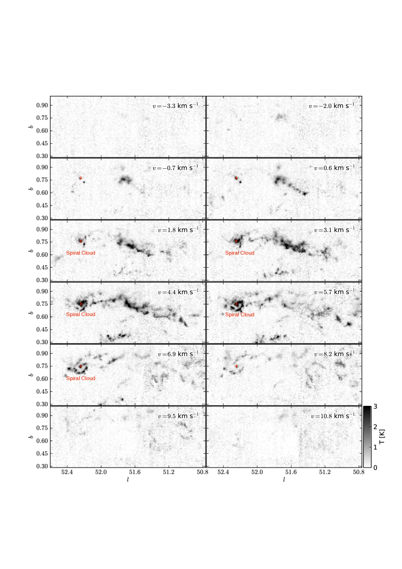
Figure 9: ¹³CO(1-0) channel maps of the cloud complex. The red “$+$” marker indicate the centre of the Spiral Cloud. The cloud complex belongs to a 500-pc filamentary gas wisp, which has been reported in Li et al. (2013).

Appendix B Physical Properties of the Clumps

The physical properties of the clumps are evaluated using the formalism outlined in Goodman et al. (2009). The radii of the clumps are evaluated as $R=1.91\times\sqrt{\sigma_{\rm maj}\sigma_{\rm min}}$ where $\sigma_{\rm maj}$ and $\sigma_{\rm min}$ are the major and minor axis dispersion (Solomon et al. 1987). The velocity dispersions of the clumps are evaluated using the intensity-weighted standard deviation of velocities of all vorxels that belong to the clumps. The column densities of the clumps are evaluated as $\Sigma=M/\pi R^{2}$. The physical properties of the clumps are listed in Table 1.

Table 1: Properties of the ¹³CO Clumps

ID	Mass	Gal. Lon.	Gal. Lat.	vlsr	Radius	Velocity Dispersion	Viral Parameter	Spiral arm
	($M_{\odot}$)	(Degree)	(Degree)	($\rm km\;s^{-1}$)	(parsec)	($\rm km\;s^{-1}$)
0	$1.3\text{\times}{10}^{03}$	52.20	0.73	0.94	1.76	1.10	1.8	False
1	$2.4\text{\times}{10}^{02}$	52.19	0.80	2.37	1.18	0.42	1.0	True
2	$8.0\text{\times}{10}^{03}$	52.23	0.76	4.33	3.67	1.05	0.6	True
3	$1.8\text{\times}{10}^{03}$	52.08	0.77	3.75	4.27	0.74	1.4	False
4	$3.2\text{\times}{10}^{03}$	52.21	0.69	5.02	2.95	0.94	0.9	True
5	$3.6\text{\times}{10}^{02}$	52.00	0.78	4.03	1.80	0.41	1.0	False
6	$3.4\text{\times}{10}^{03}$	52.30	0.70	5.81	4.26	0.90	1.1	True
7	$1.8\text{\times}{10}^{03}$	52.18	0.73	5.52	2.97	0.69	0.9	True
8	$4.2\text{\times}{10}^{02}$	52.13	0.73	4.76	2.04	0.38	0.8	False
9	$3.7\text{\times}{10}^{02}$	52.18	0.78	5.08	1.19	0.46	0.8	True
10	$7.8\text{\times}{10}^{02}$	52.01	0.86	5.54	2.28	0.79	2.1	False
11	$3.3\text{\times}{10}^{02}$	52.19	0.66	5.39	1.41	0.41	0.8	False
12	$2.0\text{\times}{10}^{03}$	52.38	0.72	6.44	3.28	0.88	1.4	False
13	$3.6\text{\times}{10}^{02}$	52.42	0.63	6.76	2.08	0.79	4.0	False
14	$1.8\text{\times}{10}^{02}$	52.08	0.84	6.44	1.51	0.76	5.5	False
15	$3.1\text{\times}{10}^{02}$	52.27	0.67	6.96	1.70	0.38	0.9	True

Appendix C Analysis of the structure

To analyse its structure we divide the cloud into different rings. The positions of the rings are presented in Fig. 10, and in Fig. 11 we present the velocity structure of the cloud inside these rings.

We adopt a systemic velocity of 5 $\rm km/s$ for the Spiral Cloud. For each position, the FHWMs of the emission lines are determined by ${\rm FWHM}\approx 0.93I/T_{\rm peak}$ where $I$ is the integrated intensity, and $T_{\rm peak}$ is the peak the emission line.

We also compare the observational data with a model of a flat rotating disk model (Mestel 1963), described in detail in Sect. 3.2. The model has a constant circular velocity (flat rotation profile), characterised by $v_{\rm circ}$, which is 6.6 $\rm km/s$ (Eq. 2). Assuming an inclination of 45^∘, we derive the observed velocity signature of such a model.

At the very inner regions (up to $r_{\rm cloud}=7.48\;\rm pc$), the observed lines are sometimes not purely Gaussian. This might lead to some underestimates of the column density, and might make the velocity centroid estimates inaccurate. Indeed, the line profiles are more irregular at the region $l\approx 52.26^{\circ}$, $b\approx 0.76^{\circ}$ where the line widths are much higher (Fig. 14). A few causes for the irregular line profiles are possible, such as line of sight superposition and opacity broadening. If the latter is dominating, the deviation of our model from the model of Mestel (1963) would be smaller than Fig. 3 suggests.

Another uncertainty in our modelling is the distance. The expected rotational velocity is linked to $r_{0}$ by Eq. 2, and $r_{0}$ is proportional to the distance. Since the distance used in our analysis is the kinematic distance, whose uncertainty is typically 20 %, we expect a similar uncertainty to exist in the expected rotational velocity. The expected velocity shift is also dependent on the assumed inclination of the cloud.

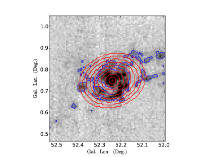
Figure 10: A demonstration of our ring-based analysis of the cloud. The spacing of the rings are 2.7 pc, which is comparable to the beam size (which is 2.2 pc). The blue solid lines stand for the region within which the emission is analysed. The cut was made at $\int T_{A*}{\rm d}{\rm v}=5.1\;\rm km/s$, This corresponds to 3.5 times the rms noise level. The red contours denote the boundaries of the rings that we use to divide and analyse the kinematic structure of the Spiral Cloud.

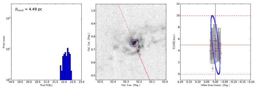
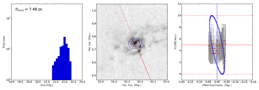
Figure 11: Structure of the cloud viewed within rings. On the left panels, we present the distributions of estimated $\rm H_{2}$ column densities of the pixels. The mean radii of the rings ($r_{\rm cloud}$) are indicated at the upper left corners of each panel. In the middle panels, we plot the boundaries of the rings. The proposed rotational axis is represented by the red lines. The red solid lines represent parts of the rotational axes that are in front of the cloud, and the red dashed lines represent parts of the rotational axes that are at the back of the cloud. the right panels we present the velocity centroids of the emission in the position-velocity space. Here, we have projected individual line of sight observations onto the major axis of ellipsoid representing the cloud, and the x-axes are the projected offests from the centres. The horizontal lines in the right panels denote the range of velocities within which the gas is gravitationally bound to the cloud. For each line of sight, we plot the velocity centroids and the FWHMs. The centroids of the emission lines are represented as the red symbols, and the FWHMs of the of the emission lines are represented as the errorbars. The horizontal red lines represent the systemic velocity of the cloud, which is $5\;\rm km/s$. The blue curve is the expected rotational signature assuming the balance between rotation and gravity (Sec. 3.2). The vertical blue lines in the middle and right panels indicate the centre of the cloud. This figure is to be continued in the next page.

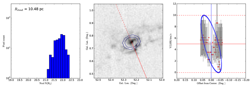
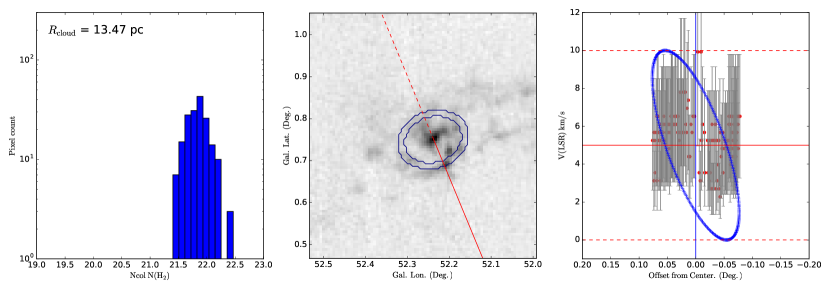
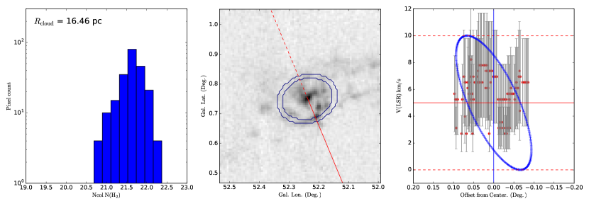
Figure 12: A continuation of Fig. 11.

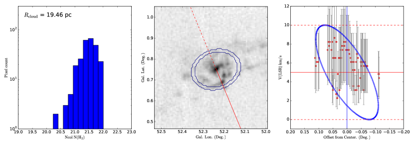
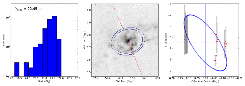
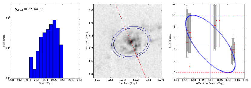
Figure 13: A continuation of Fig. 11, 12.

Appendix D Detailed velocity structure of the spiral cloud

In Fig. 14 we present the velocity centroid map and the velocity FWHM map of the cloud.

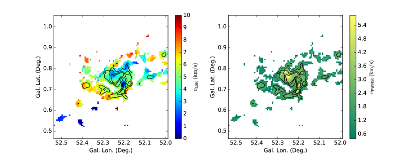
Figure 14: Detailed velocity structure of the spiral cloud. The left panel shows the velocity centroid map, and the right panel shows the velocity FWHM map. Overlaid contours are velocity-integrated ¹³CO(1-0) emission, and the levels correspond to 5.1, 10.2, 15.3 $\rm K\;km\;s^{-1}$. In producing these maps, we have excluded vorxels where the emission is below 0.43 K, which corresponds to three times the rms noise level of the data cube.

References

- Abreu-Vicente et al. (2016) Abreu-Vicente, J., Ragan, S., Kainulainen, J., et al. 2016, A&A, 590, A131
- Ballesteros-Paredes et al. (2012) Ballesteros-Paredes, J., D’Alessio, P., & Hartmann, L. 2012, MNRAS, 427, 2562
- Ballesteros-Paredes et al. (1999) Ballesteros-Paredes, J., Hartmann, L., & Vázquez-Semadeni, E. 1999, ApJ, 527, 285
- Ballesteros-Paredes et al. (2011) Ballesteros-Paredes, J., Hartmann, L. W., Vázquez-Semadeni, E., Heitsch, F., & Zamora-Avilés, M. A. 2011, MNRAS, 411, 65
- Bania et al. (2012) Bania, T. M., Anderson, L. D., & Balser, D. S. 2012, ApJ, 759, 96
- Bastien (1983) Bastien, P. 1983, A&A, 119, 109
- Benjamin et al. (2003) Benjamin, R. A., Churchwell, E., Babler, B. L., et al. 2003, PASP, 115, 953
- Bertoldi & McKee (1992) Bertoldi, F. & McKee, C. F. 1992, ApJ, 395, 140
- Binney & Tremaine (2008) Binney, J. & Tremaine, S. 2008, Galactic Dynamics: Second Edition (Princeton University Press)
- Bodenheimer (1978) Bodenheimer, P. 1978, ApJ, 224, 488
- Carey et al. (2009) Carey, S. J., Noriega-Crespo, A., Mizuno, D. R., et al. 2009, PASP, 121, 76
- Dale et al. (2009) Dale, J. E., Wünsch, R., Whitworth, A., & Palouš, J. 2009, MNRAS, 398, 1537
- Dobbs (2015) Dobbs, C. L. 2015, MNRAS, 447, 3390
- Dobbs et al. (2014) Dobbs, C. L., Krumholz, M. R., Ballesteros-Paredes, J., et al. 2014, Protostars and Planets VI, 3
- Elmegreen & Elmegreen (1983) Elmegreen, B. G. & Elmegreen, D. M. 1983, MNRAS, 203, 31
- Elmegreen & Lada (1977) Elmegreen, B. G. & Lada, C. J. 1977, ApJ, 214, 725
- Goodman et al. (1993) Goodman, A. A., Benson, P. J., Fuller, G. A., & Myers, P. C. 1993, ApJ, 406, 528
- Goodman et al. (2009) Goodman, A. A., Rosolowsky, E. W., Borkin, M. A., et al. 2009, Nature, 457, 63
- Heitsch & Hartmann (2008) Heitsch, F. & Hartmann, L. 2008, ApJ, 689, 290
- Hennebelle & Falgarone (2012) Hennebelle, P. & Falgarone, E. 2012, A&A Rev., 20, 55
- Heyer & Dame (2015) Heyer, M. & Dame, T. M. 2015, ARA&A, 53, 583
- Heyer et al. (2009) Heyer, M., Krawczyk, C., Duval, J., & Jackson, J. M. 2009, ApJ, 699, 1092
- Hoyle (1953) Hoyle, F. 1953, ApJ, 118, 513
- Imara et al. (2011) Imara, N., Bigiel, F., & Blitz, L. 2011, ApJ, 732, 79
- Jackson et al. (2006) Jackson, J. M., Rathborne, J. M., Shah, R. Y., et al. 2006, ApJS, 163, 145
- Kauffmann et al. (2010) Kauffmann, J., Pillai, T., Shetty, R., Myers, P. C., & Goodman, A. A. 2010, ApJ, 716, 433
- Klessen & Hennebelle (2010) Klessen, R. S. & Hennebelle, P. 2010, A&A, 520, A17
- Krumholz & McKee (2005) Krumholz, M. R. & McKee, C. F. 2005, ApJ, 630, 250
- Larson (1973) Larson, R. B. 1973, ARA&A, 11, 219
- Li (2014) Li, G.-X. 2014, PhD thesis, Rheinische Friedrich-Wilhelms-Universitat Bonn
- Li et al. (2016) Li, G.-X., Urquhart, J. S., Leurini, S., et al. 2016, A&A, 591, A5
- Li et al. (2013) Li, G.-X., Wyrowski, F., Menten, K., & Belloche, A. 2013, A&A, 559, A34
- Li et al. (2014) Li, H.-B., Goodman, A., Sridharan, T. K., et al. 2014, Protostars and Planets VI, 101
- Li et al. (2015) Li, H.-B., Yuen, K. H., Otto, F., et al. 2015, Nature, 520, 518
- Liu et al. (2015) Liu, H. B., Galván-Madrid, R., Jiménez-Serra, I., et al. 2015, ApJ, 804, 37
- Lockman (1989) Lockman, F. J. 1989, ApJS, 71, 469
- Mac Low & Klessen (2004) Mac Low, M.-M. & Klessen, R. S. 2004, Reviews of Modern Physics, 76, 125
- Mercer et al. (2005) Mercer, E. P., Clemens, D. P., Meade, M. R., et al. 2005, ApJ, 635, 560
- Mestel (1963) Mestel, L. 1963, MNRAS, 126, 553
- Padoan & Nordlund (1999) Padoan, P. & Nordlund, Å. 1999, ApJ, 526, 279
- Phillips (1999) Phillips, J. P. 1999, A&AS, 134, 241
- Pringle et al. (2001) Pringle, J. E., Allen, R. J., & Lubow, S. H. 2001, MNRAS, 327, 663
- Ragan et al. (2014) Ragan, S. E., Henning, T., Tackenberg, J., et al. 2014, A&A, 568, A73
- Ridge et al. (2006) Ridge, N. A., Di Francesco, J., Kirk, H., et al. 2006, AJ, 131, 2921
- Roman-Duval et al. (2010) Roman-Duval, J., Jackson, J. M., Heyer, M., Rathborne, J., & Simon, R. 2010, ApJ, 723, 492
- Rosolowsky (2007) Rosolowsky, E. 2007, ApJ, 654, 240
- Rosolowsky et al. (2008) Rosolowsky, E. W., Pineda, J. E., Kauffmann, J., & Goodman, A. A. 2008, ApJ, 679, 1338
- Schuller et al. (2009) Schuller, F., Menten, K. M., Contreras, Y., et al. 2009, A&A, 504, 415
- Simon et al. (2001) Simon, R., Jackson, J. M., Clemens, D. P., Bania, T. M., & Heyer, M. H. 2001, ApJ, 551, 747
- Smith et al. (2014) Smith, R. J., Glover, S. C. O., Clark, P. C., Klessen, R. S., & Springel, V. 2014, MNRAS, 441, 1628
- Solomon et al. (1987) Solomon, P. M., Rivolo, A. R., Barrett, J., & Yahil, A. 1987, ApJ, 319, 730
- Thompson et al. (2012) Thompson, M. A., Urquhart, J. S., Moore, T. J. T., & Morgan, L. K. 2012, MNRAS, 421, 408
- Toomre (1964) Toomre, A. 1964, ApJ, 139, 1217
- Urquhart et al. (2009) Urquhart, J. S., Hoare, M. G., Purcell, C. R., et al. 2009, A&A, 501, 539
- Urquhart et al. (2013) Urquhart, J. S., Thompson, M. A., Moore, T. J. T., et al. 2013, MNRAS, 435, 400
- Utomo et al. (2015) Utomo, D., Blitz, L., Davis, T., et al. 2015, ApJ, 803, 16
- Wang et al. (2015) Wang, K., Testi, L., Ginsburg, A., et al. 2015, MNRAS, 450, 4043
- Whitworth et al. (1994) Whitworth, A. P., Bhattal, A. S., Chapman, S. J., Disney, M. J., & Turner, J. A. 1994, A&A, 290, 421
- Whitworth & Francis (2002) Whitworth, A. P. & Francis, N. 2002, MNRAS, 329, 641
- Wienen et al. (2015) Wienen, M., Wyrowski, F., Menten, K. M., et al. 2015, A&A, 579, A91
- Williams et al. (1994) Williams, J. P., de Geus, E. J., & Blitz, L. 1994, ApJ, 428, 693
- Zinnecker (1984) Zinnecker, H. 1984, MNRAS, 210, 43
- Zucker et al. (2015) Zucker, C., Battersby, C., & Goodman, A. 2015, ApJ, 815, 23