The relation of the Dzyaloshinskii-Moriya interaction to spin currents and to the spin-orbit field

Abstract

Starting from the general Berry phase theory of the Dzyaloshinskii-Moriya interaction (DMI) we derive an expression for the linear contribution of the spin-orbit interaction (SOI). Thereby, we show analytically that at the first order in SOI DMI is given by the ground-state spin current. We verify this finding numerically by ab-initio calculations in Mn/W(001) and Co/Pt(111) magnetic bilayers. We show that despite the strong SOI from the 5$d$ heavy metals DMI is well-approximated by the first order in SOI, while the ground-state spin current is not. We decompose the SOI-linear contribution to DMI into two parts. One part has a simple interpretation in terms of the Zeeman interaction between the spin-orbit field and the spin misalignment that electrons acquire in magnetically noncollinear textures. This interpretation provides also an intuitive understanding of the symmetry of DMI on the basis of the spin-orbit field and it explains in a simple way why DMI and ground-state spin currents are related. Moreover, we show that energy currents driven by magnetization dynamics and associated to DMI can be explained by counter-propagating spin currents that carry energy due to their Zeeman interaction with the spin-orbit field. Finally, we discuss options to modify DMI by nonequilibrium spin currents excited by electric fields or light.

I Introduction

Most excitement about spin-currents arises from the prospects to use them to transmit information dissipationlessly Murakami et al. (2003), to switch magnetic bits Liu et al. (2012); Mihai Miron et al. (2011) and to move domain walls Thomas et al. (2013); Emori et al. (2013). Therefore, in many cases the generation of spin currents by applied electric fields, i.e., the spin Hall effect Sinova et al. (2015), or by magnetization dynamics, i.e., spin-pumping Tserkovnyak et al. (2002), or by laser excitation Kampfrath et al. (2013) are considered. However, spin currents exist also in the absence of applied electric fields, magnetization dynamics and laser pulses, when the system is in its ground state. These ground-state spin currents mediate important effects and interactions as well. For example, in magnetic bilayer systems the ground-state spin current flowing between the magnetic layer and the normal metal substate when the magnetization is tilted away from the easy axis provides the nonlocal contribution to the magnetic anisotropy torque Freimuth et al. (2014a). Furthermore, the interlayer exchange coupling between magnetic layers in spin valves is mediated by ground-state spin currents Haney et al. (2009).

Recently, it has been proposed to estimate the Dzyaloshinskii-Moriya interaction (DMI) from the ground-state spin current Kikuchi et al. (2016). DMI describes the linear-in-$q$ contribution to the energy dispersion $E(q)$ of spin-spirals and arises in systems with inversion asymmetry and spin-orbit interaction (SOI) Moriya (1960); Dzyaloshinsky (1958). In several spintronics concepts DMI plays a central role. Notably, it is a key ingredient to achieve current-driven domain wall motion at high speed Thomas et al. (2013); Emori et al. (2013) and to stabilize skyrmions Rößler et al. (2006). The relation of DMI to the ground-state spin current also leads to an intuitive interpretation of DMI as a Doppler shift Kikuchi et al. (2016).

Since the computational evaluation of the ground-state spin current is easier than the usually applied methodology for the calculation of the DMI coefficients from the $q$-linear contribution to the energy dispersion $E({\bm{q}})$ of spin spirals Heide et al. (2008); Ferriani et al. (2008); Heide et al. (2009); Yang et al. (2015), it has been proposed to use the ground-state spin currents for example to study the dependence of DMI on strain and voltage Kikuchi et al. (2016). However, the relation between DMI and ground-state spin current has been derived in the strong exchange limit and the accuracy of this spin-current approach to DMI has been demonstrated only in the B20 compounds Mn_1-xFe_xGe and Fe_1-xCo_xGe. In Co/Pt magnetic bilayer systems SOI is much stronger than in these B20 compounds and the applicability of the spin-current approach to such magnetic bilayer systems has not been demonstrated yet.

The description of ferroelectric polarization by the Berry phase Vanderbilt and King-Smith (1993), the use of the Berry curvature in the theory of the anomalous Hall effect Nagaosa et al. (2010), and the discovery of topological insulators are well-known examples for the success story of the quest for effects of topological and geometrical origin in band theory. Recently, it has been shown that the exchange parameters can be expressed in terms of geometrical properties such as the quantum metrics Freimuth et al. (2017) and that DMI can be expressed in terms of the mixed Berry curvature ${\rm Im}\langle\partial u_{{\bm{k}}n}/\partial\hat{{\bm{n}}}|\partial u_{{\bm{k}}n}/\partial{\bm{k}}\rangle$, where derivatives with respect to the $k$-point and derivatives with respect to the magnetization direction $\hat{{\bm{n}}}$ are combined Freimuth et al. (2014b, 2013, 2016).

This Berry phase approach expresses DMI directly in terms of the electronic structure, similar to the spin-current approach. This is a major advantage of these two approaches compared to the spin-spiral method, where DMI is extracted from the $q$-linear contribution to the energy dispersion $E({\bm{q}})$ of spin spirals. While the relation of DMI to other important spintronics effects is not directly obvious within the spin-spiral approach, the Berry phase theory of DMI shows how DMI is related to direct, inverse and thermal spin-orbit torques and to the twist-torque moments of wave-packets Freimuth et al. (2013, 2014b, 2016). Since the spin-current approach to DMI establishes the connection to the ground-state spin current, even more insights can be expected from investigating the relationship between the Berry phase approach on the one hand and the spin current approach on the other hand.

In the present paper we use first-order perturbation theory to derive expressions for DMI and for the ground-state spin current, which are valid at the first order in SOI. Thereby we find analytically that DMI is given exactly by the ground-state spin current at the first order in SOI, which clarifies the relation between the Berry-phase approach and the spin-current approach to DMI. Tuning the SOI strength in Co/Pt(111) and Mn/W(001) magnetic bilayers artificially we confirm this analytical result numerically by ab-initio calculations. By studying both DMI and ground-state spin current as a function of SOI strength we illustrate the limitations of the spin-current approach to DMI, which breaks down for large SOI strength. We find that the SOI-linear contribution to the ground-state spin current consists of two terms, and provide an intuitive interpretation of both of them. We discover that one contribution is intimately linked to the misalignment that conduction electron spins acquire as they traverse magnetically noncollinear textures. This contribution can be understood as Zeeman interaction between the spin-orbit field and the spin misalignment. When the magnetization direction is time-dependent, the spin misalignment leads to counterpropagating spin currents, based on which we elucidate the nature of the energy current that is driven by magnetization dynamics in systems with DMI Freimuth et al. (2016). Thereby our theory exposes the connections of DMI to other spintronics concepts such as spin-orbit fields and spin-transfer torque.

This article is structured as follows. In section II we derive expressions for the SOI-linear contributions to DMI and to the ground-state spin current and show that both agree within the first order perturbation theory in SOI. In section III.1 and III.2 we interpret the two contributions to DMI that arise at the first order in SOI. In section IV we explain how the ground-state energy current associated with DMI can be understood from counter-propagating spin currents driven by magnetization dynamics. In section V we show that ground-state spin currents exist for the nonmagnetic Rashba model with zero DMI, but that these spin currents arise at the third order of SOI. In section VI we present ab-initio calculations of DMI and of ground-state spin currents in Mn/W(001) and Co/Pt(111) magnetic bilayers. In section VII we conclude with a summary and outlook, where we also discuss the option to modify DMI by nonequilibrium spin currents excited by electric fields or light.

II First-order contribution of SOI to DMI

Due to DMI the free energy density $F({\bm{r}})$ at position ${\bm{r}}$ contains a term linear in the gradients of magnetization Freimuth et al. (2014b):

$$F^{\rm DMI}({\bm{r}})=\sum_{j}{\bm{D}}_{j}(\hat{{\bm{n}}}({\bm{r}}))\cdot\left[\hat{{\bm{n}}}({\bm{r}})\times\frac{\partial\hat{{\bm{n}}}({\bm{r}})}{\partial r_{j}}\right],$$ (1)

where ${\bm{D}}_{j}(\hat{{\bm{n}}})$ are the DMI coefficient vectors, which depend on the magnetization direction $\hat{{\bm{n}}}({\bm{r}})$ in systems where DMI is anisotropic. The index $j$ runs over the three cartesian directions $x$, $y$ and $z$.

Within the Berry phase approach ${\bm{D}}_{j}(\hat{{\bm{n}}})$ is given by

$${\bm{D}}_{j}(\hat{{\bm{n}}})\!=\!\!\!\int\!\!\!\frac{{\rm d}^{d}k}{(2\pi)^{d}}\sum_{n}\Bigl{[}f(\mathcal{E}_{{\bm{k}}n}){\bm{A}}_{{\bm{k}}nj}(\hat{{\bm{n}}})-g(\mathcal{E}_{{\bm{k}}n}){\bm{B}}_{{\bm{k}}nj}(\hat{{\bm{n}}})\Bigr{]},$$ (2)

where $d$ is the dimension ($d$=2 or $d$=3), $f(\mathcal{E}_{{\bm{k}}n})=[1+e^{\beta(\mathcal{E}_{{\bm{k}}n}-\mu)}]^{-1}$ is the occupation number of band $n$ at $k$ point ${\bm{k}}$, $g(\mathcal{E}_{{\bm{k}}n})=-k_{\rm B}T\ln[1+e^{-\beta(\mathcal{E}_{{\bm{k}}n}-\mu)}]$ is the contribution of the state $|u_{{\bm{k}}n}\rangle$ with band energy $\mathcal{E}_{{\bm{k}}n}$ to the grand canonical potential, $T$ is the temperature, $k_{\rm B}$ is Boltzmann’s constant, $\mu$ is the chemical potential and $\beta=(k_{\rm B}T)^{-1}$. In the mixed Berry curvature Freimuth et al. (2013)

$${\bm{B}}_{{\bm{k}}nj}(\hat{{\bm{n}}})=-2\left[\hat{{\bm{n}}}\times{\rm Im}\left\langle\frac{\partial u_{{\bm{k}}n}}{\partial\hat{{\bm{n}}}}\left|\frac{\partial u_{{\bm{k}}n}}{\partial k_{j}}\right.\right\rangle\right]$$ (3)

${\bm{k}}$-derivatives are mixed with $\hat{{\bm{n}}}$-derivatives. The twist-torque moment of wavepackets is described by Freimuth et al. (2014b)

$${\bm{A}}_{{\bm{k}}nj}(\hat{{\bm{n}}})=-\left[\hat{{\bm{n}}}\times{\rm Im}\left\langle\frac{\partial u_{{\bm{k}}n}}{\partial\hat{{\bm{n}}}}\right|\!\Bigl{[}\mathcal{E}_{{\bm{k}}n}-H_{{\bm{k}}}\Bigr{]}\!\left|\frac{\partial u_{{\bm{k}}n}}{\partial k_{j}}\right\rangle\right],$$ (4)

where $H_{{\bm{k}}}$ is the Hamiltonian in crystal-momentum representation, i.e., $H_{{\bm{k}}}|u_{{\bm{k}}n}\rangle=\mathcal{E}_{{\bm{k}}n}|u_{{\bm{k}}n}\rangle$.

In the limit of strong exchange or small SOI the DMI coefficient vector ${\bm{D}}_{j}$ can also be determined from the ground-state spin current ${\bm{Q}}_{j}$ Katsnelson et al. (2010); Kikuchi et al. (2016). When the ground-state spin current flowing in $j$ direction is defined as

$${\bm{Q}}_{j}=\frac{\hbar}{4}\int\!\!\frac{{\rm d}^{d}k}{(2\pi)^{d}}\sum_{n}f(\mathcal{E}_{{\bm{k}}n})\left\langle u_{{\bm{k}}n}\right|\{{\bm{\sigma}},v_{j}\}\left|u_{{\bm{k}}n}\right\rangle,$$ (5)

the DMI coefficient vector can be written as

$${\bm{D}}_{j}=-{\bm{Q}}_{j}.$$ (6)

Here, $v_{j}$ is the $j$ component of the velocity operator ${\bm{v}}$ and ${\bm{\sigma}}=(\sigma_{x},\sigma_{y},\sigma_{z})^{\rm T}$ is the vector of Pauli spin matrices.

Both Eq. (2) and Eq. (5) express the DMI directly in terms of the electronic structure, which is a major advantage over the spin-spiral method, where DMI is extracted from the $q$-linear term in the energy dispersion Heide et al. (2008); Ferriani et al. (2008); Heide et al. (2009); Yang et al. (2015). However, Eq. (2) and Eq. (5) look very different and the relationship between both approaches is not clear. Since DMI arises at the first order in SOI Moriya (1960), we will use first-order perturbation theory to determine the SOI-linear contributions to ${\bm{D}}_{j}$ and ${\bm{Q}}_{j}$. This will facilitate the comparison between the approaches Eq. (2) and Eq. (5) and elucidate their relationship.

Within Kohn-Sham density functional theory interacting many-electron systems are described by the effective single-particle Hamiltonian

$$H({\bm{r}}) =-\frac{\hbar^{2}}{2m}\Delta+V({\bm{r}})+\mu_{\rm B}{\bm{\sigma}}\cdot\hat{{\bm{n}}}\Omega^{\rm xc}({\bm{r}})+$$ (7)

$$+\frac{1}{2ec^{2}}\mu_{\rm B}{\bm{\sigma}}\cdot\left[{\bm{\nabla}}V({\bm{r}})\times{\bm{v}}\right],$$

where the first term describes the kinetic energy and the second term is the scalar effective potential. The third term describes the exchange interaction, where $\mu_{\rm B}$ is the Bohr magneton, $\Omega^{\rm xc}({\bm{r}})=\frac{1}{2\mu_{\rm B}}\left[V^{\rm eff}_{\rm minority}({\bm{r}})-V^{\rm eff}_{\rm majority}({\bm{r}})\right]$ is the exchange field, $V^{\rm eff}_{\rm minority}({\bm{r}})$ is the effective potential of minority electrons and $V^{\rm eff}_{\rm majority}({\bm{r}})$ is the effective potential of majority electrons. The last term is the spin-orbit interaction, where $e$ is the elementary positive charge and $c$ is the velocity of light.

The Hamiltonian in crystal-momentum representation is given by $H_{{\bm{k}}}=e^{-i{\bm{k}}\cdot{\bm{r}}}He^{i{\bm{k}}\cdot{\bm{r}}}$. We decompose $H_{{\bm{k}}}$ into the spin-orbit interaction $\mathcal{V}_{{\bm{k}}}$ and the Hamiltonian $\bar{H}_{{\bm{k}}}$ without SOI, such that

$$H_{{\bm{k}}}=\bar{H}_{{\bm{k}}}+\mathcal{V}_{{\bm{k}}}.$$ (8)

We introduce the parameter $\xi$ to scale SOI up or down and consider the modified Hamiltonian

$$H_{{\bm{k}}}^{\xi}=\bar{H}_{{\bm{k}}}+\xi\mathcal{V}_{{\bm{k}}}.$$ (9)

The DMI coefficient vector ${\bm{D}}_{j}$ of a system described by $H_{{\bm{k}}}^{\xi}$ can be written as a power series with respect to $\xi$:

$${\bm{D}}_{j}=\xi{\bm{D}}^{(1)}_{j}+\xi^{2}{\bm{D}}^{(2)}_{j}+\xi^{3}{\bm{D}}^{(3)}_{j}+\dots,$$ (10)

where ${\bm{D}}^{(1)}_{j}$ is linear in $\mathcal{V}_{{\bm{k}}}$.

In order to derive an explicit expression for ${\bm{D}}^{(1)}_{j}$ it is convenient to rewrite Eq. (2) in terms of Green functions. This can be achieved by first expressing the ${\bm{k}}$ and $\hat{{\bm{n}}}$ derivatives through the velocity and torque operators, respectively. For this purpose we employ $\hbar{\bm{v}}=\partial H/\partial{\bm{k}}$ and $\hat{{\bm{n}}}\times\partial H/\partial\hat{{\bm{n}}}={\bm{\mathcal{T}}}$ and use perturbation theory in order to rewrite the ${\bm{k}}$ and $\hat{{\bm{n}}}$ derivatives in terms of matrix elements of ${\bm{v}}$ and ${\bm{\mathcal{T}}}$ Freimuth et al. (2014a, 2013). This yields

$${\bm{A}}_{{\bm{k}}nj}=\hbar\sum_{m\neq n}\text{Im}\left[\frac{\langle u_{{\bm{k}}n}|{\bm{\mathcal{T}}}|u_{{\bm{k}}m}\rangle\langle u_{{\bm{k}}m}|v_{j}|u_{{\bm{k}}n}\rangle}{\mathcal{E}_{{\bm{k}}m}-\mathcal{E}_{{\bm{k}}n}}\right]$$ (11)

and

$${\bm{B}}_{{\bm{k}}nj}=-2\hbar\sum_{m\neq n}\text{Im}\left[\frac{\langle u_{{\bm{k}}n}|{\bm{\mathcal{T}}}|u_{{\bm{k}}m}\rangle\langle u_{{\bm{k}}m}|v_{j}|u_{{\bm{k}}n}\rangle}{(\mathcal{E}_{{\bm{k}}m}-\mathcal{E}_{{\bm{k}}n})^{2}}\right],$$ (12)

where

$${\bm{\mathcal{T}}}=\frac{i}{2}\left[\bar{H}_{{\bm{k}}},{\bm{\sigma}}\right]=-\mu_{\rm B}{\bm{\sigma}}\times\hat{{\bm{n}}}\Omega^{\rm xc}$$ (13)

is the torque operator Freimuth et al. (2015). Subsequently, we apply the identity

$${\rm Im}\int{\rm d}\mathcal{E}g(\mathcal{E})\frac{1}{\mathcal{E}-\mathcal{E}_{{\bm{k}}q}+i0^{+}}\frac{1}{(\mathcal{E}-\mathcal{E}_{{\bm{k}}p}+i0^{+})^{2}}=$$ (14)

$$=\pi\left[\frac{[g(\mathcal{E}_{{\bm{k}}p})-g(\mathcal{E}_{{\bm{k}}q})]}{(\mathcal{E}_{{\bm{k}}p}-\mathcal{E}_{{\bm{k}}q})^{2}}+\frac{f(\mathcal{E}_{{\bm{k}}p})}{\mathcal{E}_{{\bm{k}}q}-\mathcal{E}_{{\bm{k}}p}}\right],$$

which can be proven with the residue theorem and with the relation $g^{\prime}(\mathcal{E})=f(\mathcal{E})$. Thereby, we obtain the following expression of the DMI coefficients in terms of Green functions not :

$$\begin{aligned} &{\bm{D}}_{j}=\frac{1}{h}{\rm Re}\int\frac{{\rm d}^{d}k}{(2\pi)^{d}}\int{\rm d}\mathcal{E}g(\mathcal{E})\times\\ &\times{\rm Tr}\left[{\bm{\mathcal{T}}}G_{{\bm{k}}}^{\rm R}(\mathcal{E})v_{j}\frac{dG_{{\bm{k}}}^{\rm R}(\mathcal{E})}{d\mathcal{E}}-{\bm{\mathcal{T}}}\frac{dG_{{\bm{k}}}^{\rm R}(\mathcal{E})}{d\mathcal{E}}v_{j}G_{{\bm{k}}}^{\rm R}(\mathcal{E})\right],\end{aligned}$$ (15)

where $G_{{\bm{k}}}^{\rm R}(\mathcal{E})=\hbar\left[\mathcal{E}-H_{{\bm{k}}}+i0^{+}\right]^{-1}$ is the retarded Green function.

In order to identify the contributions to Eq. (15) that are linear in SOI we expand $G_{{\bm{k}}}^{\rm R}(\mathcal{E})$ up to first order in $\mathcal{V}_{{\bm{k}}}$ as follows:

$$G^{\rm R}_{{\bm{k}}}(\mathcal{E})\simeq\bar{G}^{\rm R}_{{\bm{k}}}(\mathcal{E})+\frac{1}{\hbar}\bar{G}^{\rm R}_{{\bm{k}}}(\mathcal{E})\mathcal{V}_{{\bm{k}}}\bar{G}^{\rm R}_{{\bm{k}}}(\mathcal{E}),$$ (16)

where $\bar{G}_{{\bm{k}}}^{\rm R}(\mathcal{E})=\hbar\left[\mathcal{E}-\bar{H}_{{\bm{k}}}+i0^{+}\right]^{-1}$ is the retarded Green function without SOI. Additionally, we decompose the velocity operator into two parts:

$$v_{j}=\bar{v}_{j}+v^{\rm SOI}_{j},$$ (17)

where $\bar{v}_{j}=i[\bar{H}_{{\bm{k}}},r_{j}]/\hbar$ and $v^{\rm SOI}_{j}=i[\mathcal{V}_{{\bm{k}}},r_{j}]/\hbar$. Inserting Eq. (16) and Eq. (17) into Eq. (15) and using the relation $\hbar\partial\bar{G}^{\rm R}_{{\bm{k}}}(\mathcal{E})/\partial\mathcal{E}=-[\bar{G}^{\rm R}_{{\bm{k}}}(\mathcal{E})]^{2}$ we obtain the linear contribution of SOI to ${\bm{D}}_{j}$:

$$\begin{aligned} {\bm{D}}^{(1)}_{j}=&\frac{-1}{2\pi\hbar^{3}}{\rm Re}\int\frac{{\rm d}^{d}k}{(2\pi)^{d}}\int{\rm d}\mathcal{E}g(\mathcal{E}){\rm Tr}\Biggl{[}\\ &\bar{G}_{{\bm{k}}}^{\rm R}(\mathcal{E})\mathcal{V}_{{\bm{k}}}\bar{G}_{{\bm{k}}}^{\rm R}(\mathcal{E}){\bm{\mathcal{T}}}\bar{G}_{{\bm{k}}}^{\rm R}(\mathcal{E})\bar{v}_{j}\bar{G}_{{\bm{k}}}^{\rm R}(\mathcal{E})\\ +&\bar{G}_{{\bm{k}}}^{\rm R}(\mathcal{E}){\bm{\mathcal{T}}}\bar{G}_{{\bm{k}}}^{\rm R}(\mathcal{E})\mathcal{V}_{{\bm{k}}}\bar{G}_{{\bm{k}}}^{\rm R}(\mathcal{E})\bar{v}_{j}\bar{G}_{{\bm{k}}}^{\rm R}(\mathcal{E})\\ +&\bar{G}_{{\bm{k}}}^{\rm R}(\mathcal{E}){\bm{\mathcal{T}}}\bar{G}_{{\bm{k}}}^{\rm R}(\mathcal{E})\bar{v}_{j}\bar{G}_{{\bm{k}}}^{\rm R}(\mathcal{E})\mathcal{V}_{{\bm{k}}}\bar{G}_{{\bm{k}}}^{\rm R}(\mathcal{E})\\ +&\hbar\bar{G}_{{\bm{k}}}^{\rm R}(\mathcal{E}){\bm{\mathcal{T}}}\bar{G}_{{\bm{k}}}^{\rm R}(\mathcal{E})v^{\rm SOI}_{j}\bar{G}_{{\bm{k}}}^{\rm R}(\mathcal{E})\\ -&\bar{G}_{{\bm{k}}}^{\rm R}(\mathcal{E})\mathcal{V}_{{\bm{k}}}\bar{G}_{{\bm{k}}}^{\rm R}(\mathcal{E})\bar{v}_{j}\bar{G}_{{\bm{k}}}^{\rm R}(\mathcal{E}){\bm{\mathcal{T}}}\bar{G}_{{\bm{k}}}^{\rm R}(\mathcal{E})\\ -&\bar{G}_{{\bm{k}}}^{\rm R}(\mathcal{E})\bar{v}_{j}\bar{G}_{{\bm{k}}}^{\rm R}(\mathcal{E})\mathcal{V}_{{\bm{k}}}\bar{G}_{{\bm{k}}}^{\rm R}(\mathcal{E}){\bm{\mathcal{T}}}\bar{G}_{{\bm{k}}}^{\rm R}(\mathcal{E})\\ -&\bar{G}_{{\bm{k}}}^{\rm R}(\mathcal{E})\bar{v}_{j}\bar{G}_{{\bm{k}}}^{\rm R}(\mathcal{E}){\bm{\mathcal{T}}}\bar{G}_{{\bm{k}}}^{\rm R}(\mathcal{E})\mathcal{V}_{{\bm{k}}}\bar{G}_{{\bm{k}}}^{\rm R}(\mathcal{E})\\ -&\hbar\bar{G}_{{\bm{k}}}^{\rm R}(\mathcal{E})v^{\rm SOI}_{j}\bar{G}_{{\bm{k}}}^{\rm R}(\mathcal{E}){\bm{\mathcal{T}}}\bar{G}_{{\bm{k}}}^{\rm R}(\mathcal{E})\Biggr{]}.\end{aligned}$$ (18)

Substituting the torque operator by the commutator of inverse Green function and Pauli matrices, i.e.,

$${\bm{\mathcal{T}}}=-\frac{i\hbar}{2}\left[[\bar{G}_{{\bm{k}}}^{\rm R}(\mathcal{E})]^{-1},{\bm{\sigma}}\right],$$ (19)

reduces the number of Green functions in each of the products by one and leaves us with

$$\begin{aligned} &{\bm{D}}^{(1)}_{j}=\frac{-1}{4\pi\hbar^{2}}{\rm Im}\int\frac{{\rm d}^{d}k}{(2\pi)^{d}}\int{\rm d}\mathcal{E}g(\mathcal{E}){\rm Tr}\Biggl{[}\\ &\bar{G}_{{\bm{k}}}^{\rm R}(\mathcal{E})\mathcal{V}_{{\bm{k}}}{\bm{\sigma}}\bar{G}_{{\bm{k}}}^{\rm R}(\mathcal{E})\bar{v}_{j}\bar{G}_{{\bm{k}}}^{\rm R}(\mathcal{E})-\bar{G}_{{\bm{k}}}^{\rm R}(\mathcal{E})\mathcal{V}_{{\bm{k}}}\bar{G}_{{\bm{k}}}^{\rm R}(\mathcal{E}){\bm{\sigma}}\bar{v}_{j}\bar{G}_{{\bm{k}}}^{\rm R}(\mathcal{E})\\ +&{\bm{\sigma}}\bar{G}_{{\bm{k}}}^{\rm R}(\mathcal{E})\mathcal{V}_{{\bm{k}}}\bar{G}_{{\bm{k}}}^{\rm R}(\mathcal{E})\bar{v}_{j}\bar{G}_{{\bm{k}}}^{\rm R}(\mathcal{E})-\bar{G}_{{\bm{k}}}^{\rm R}(\mathcal{E}){\bm{\sigma}}\mathcal{V}_{{\bm{k}}}\bar{G}_{{\bm{k}}}^{\rm R}(\mathcal{E})\bar{v}_{j}\bar{G}_{{\bm{k}}}^{\rm R}(\mathcal{E})\\ +&{\bm{\sigma}}\bar{G}_{{\bm{k}}}^{\rm R}(\mathcal{E})\bar{v}_{j}\bar{G}_{{\bm{k}}}^{\rm R}(\mathcal{E})\mathcal{V}_{{\bm{k}}}\bar{G}_{{\bm{k}}}^{\rm R}(\mathcal{E})-\bar{G}_{{\bm{k}}}^{\rm R}(\mathcal{E}){\bm{\sigma}}\bar{v}_{j}\bar{G}_{{\bm{k}}}^{\rm R}(\mathcal{E})\mathcal{V}_{{\bm{k}}}\bar{G}_{{\bm{k}}}^{\rm R}(\mathcal{E})\\ +&\hbar{\bm{\sigma}}\bar{G}_{{\bm{k}}}^{\rm R}(\mathcal{E})v^{\rm SOI}_{j}\bar{G}_{{\bm{k}}}^{\rm R}(\mathcal{E})-\hbar\bar{G}_{{\bm{k}}}^{\rm R}(\mathcal{E}){\bm{\sigma}}v^{\rm SOI}_{j}\bar{G}_{{\bm{k}}}^{\rm R}(\mathcal{E})\\ -&\bar{G}_{{\bm{k}}}^{\rm R}(\mathcal{E})\mathcal{V}_{{\bm{k}}}\bar{G}_{{\bm{k}}}^{\rm R}(\mathcal{E})\bar{v}_{j}{\bm{\sigma}}\bar{G}_{{\bm{k}}}^{\rm R}(\mathcal{E})+\bar{G}_{{\bm{k}}}^{\rm R}(\mathcal{E})\mathcal{V}_{{\bm{k}}}\bar{G}_{{\bm{k}}}^{\rm R}(\mathcal{E})\bar{v}_{j}\bar{G}_{{\bm{k}}}^{\rm R}(\mathcal{E}){\bm{\sigma}}\\ -&\bar{G}_{{\bm{k}}}^{\rm R}(\mathcal{E})\bar{v}_{j}\bar{G}_{{\bm{k}}}^{\rm R}(\mathcal{E})\mathcal{V}_{{\bm{k}}}{\bm{\sigma}}\bar{G}_{{\bm{k}}}^{\rm R}(\mathcal{E})+\bar{G}_{{\bm{k}}}^{\rm R}(\mathcal{E})\bar{v}_{j}\bar{G}_{{\bm{k}}}^{\rm R}(\mathcal{E})\mathcal{V}_{{\bm{k}}}\bar{G}_{{\bm{k}}}^{\rm R}(\mathcal{E}){\bm{\sigma}}\\ -&\bar{G}_{{\bm{k}}}^{\rm R}(\mathcal{E})\bar{v}_{j}{\bm{\sigma}}\bar{G}_{{\bm{k}}}^{\rm R}(\mathcal{E})\mathcal{V}_{{\bm{k}}}\bar{G}_{{\bm{k}}}^{\rm R}(\mathcal{E})+\bar{G}_{{\bm{k}}}^{\rm R}(\mathcal{E})\bar{v}_{j}\bar{G}_{{\bm{k}}}^{\rm R}(\mathcal{E}){\bm{\sigma}}\mathcal{V}_{{\bm{k}}}\bar{G}_{{\bm{k}}}^{\rm R}(\mathcal{E})\\ -&\hbar\bar{G}_{{\bm{k}}}^{\rm R}(\mathcal{E})v^{\rm SOI}_{j}{\bm{\sigma}}\bar{G}_{{\bm{k}}}^{\rm R}(\mathcal{E})+\hbar\bar{G}_{{\bm{k}}}^{\rm R}(\mathcal{E})v^{\rm SOI}_{j}\bar{G}_{{\bm{k}}}^{\rm R}(\mathcal{E}){\bm{\sigma}}\Biggr{]}.\end{aligned}$$ (20)

We first pick out all the terms from Eq. (20) that can be expressed in terms of the anticommutators $\{{\bm{\sigma}},\bar{v}_{j}\}$ and $\{{\bm{\sigma}},v^{\rm SOI}_{j}\}$, because we are searching for a relation of the form of Eq. (6) between DMI and the ground-state spin current and according to Eq. (5) this spin-current is given in terms of such anticommutators. The sum of these contributions is given by

$${\bm{a}}_{j}= \frac{1}{4\pi\hbar^{2}}{\rm Im}\int\!\!\frac{{\rm d}^{d}k}{(2\pi)^{d}}\int\!\!{\rm d}\mathcal{E}g(\mathcal{E})\text{Tr}\Biggl{[}$$ (21)

$$\{{\bm{\sigma}},\bar{v}_{j}\}[\bar{G}_{{\bm{k}}}^{\rm R}(\mathcal{E})]^{2}\mathcal{V}_{{\bm{k}}}\bar{G}_{{\bm{k}}}^{\rm R}(\mathcal{E})+$$

$$+ \{{\bm{\sigma}},\bar{v}_{j}\}\bar{G}_{{\bm{k}}}^{\rm R}(\mathcal{E})\mathcal{V}_{{\bm{k}}}[\bar{G}_{{\bm{k}}}^{\rm R}(\mathcal{E})]^{2}+\hbar\{{\bm{\sigma}},v^{\rm SOI}_{j}\}[\bar{G}_{{\bm{k}}}^{\rm R}(\mathcal{E})]^{2}\Biggr{]}=$$

$$= \frac{1}{4\pi\hbar}{\rm Im}\int\!\!\frac{{\rm d}^{d}k}{(2\pi)^{d}}\int\!\!{\rm d}\mathcal{E}f(\mathcal{E})\text{Tr}\Biggl{[}$$

$$\{{\bm{\sigma}},\bar{v}_{j}\}\bar{G}_{{\bm{k}}}^{\rm R}(\mathcal{E})\mathcal{V}_{{\bm{k}}}\bar{G}_{{\bm{k}}}^{\rm R}(\mathcal{E})+\hbar\{{\bm{\sigma}},v^{\rm SOI}_{j}\}\bar{G}_{{\bm{k}}}^{\rm R}(\mathcal{E})\Biggr{]},$$

where we used integration by parts and the relations $\hbar\partial\bar{G}^{\rm R}_{{\bm{k}}}(\mathcal{E})/\partial\mathcal{E}=-[\bar{G}^{\rm R}_{{\bm{k}}}(\mathcal{E})]^{2}$ and $g^{\prime}(\mathcal{E})=f(\mathcal{E})$. Carrying out the energy integrations with the help of the residue theorem we obtain ${\bm{a}}_{j}={\bm{a}}_{j}^{\rm(I)}+{\bm{a}}_{j}^{\rm(II)}$ with

$${\bm{a}}_{j}^{\rm(I)}= -\frac{\hbar}{4}{\rm Re}\int\!\!\frac{{\rm d}^{d}k}{(2\pi)^{d}}\sum_{n,m}\frac{f(\bar{\mathcal{E}}_{{\bm{k}}n})-f(\bar{\mathcal{E}}_{{\bm{k}}m})}{\bar{\mathcal{E}}_{{\bm{k}}n}-\bar{\mathcal{E}}_{{\bm{k}}m}}\times$$ (22)

$$\quad\quad\quad\times\langle\bar{u}_{{\bm{k}}n}|\{{\bm{\sigma}},\bar{v}_{j}\}|\bar{u}_{{\bm{k}}m}\rangle\langle\bar{u}_{{\bm{k}}m}|\mathcal{V}_{{\bm{k}}}|\bar{u}_{{\bm{k}}n}\rangle$$

and

$${\bm{a}}_{j}^{\rm(II)}= -\frac{\hbar}{4}{\rm Re}\int\!\!\frac{{\rm d}^{d}k}{(2\pi)^{d}}\sum_{n}f(\bar{\mathcal{E}}_{{\bm{k}}n})\langle\bar{u}_{{\bm{k}}n}|\{{\bm{\sigma}},v^{\rm SOI}_{j}\}|\bar{u}_{{\bm{k}}n}\rangle,$$ (23)

where $\bar{\mathcal{E}}_{{\bm{k}}n}$ and $|\bar{u}_{{\bm{k}}n}\rangle$ are eigenvalues and eigenfunctions of the Hamiltonian $\bar{H}_{{\bm{k}}}$ without SOI, i.e., $\bar{H}_{{\bm{k}}}|\bar{u}_{{\bm{k}}n}\rangle=\bar{\mathcal{E}}_{{\bm{k}}n}|\bar{u}_{{\bm{k}}n}\rangle$. Expanding the spin current ${\bm{Q}}_{j}$ in Eq. (5) analogously to the expansion in Eq. (10) we find

$${\bm{a}}_{j}=-{\bm{Q}}^{(1)}_{j},$$ (24)

where ${\bm{Q}}^{(1)}_{j}$ is the SOI-linear term in

$${\bm{Q}}_{j}=\xi{\bm{Q}}^{(1)}_{j}+\xi^{2}{\bm{Q}}^{(2)}_{j}+\xi^{3}{\bm{Q}}^{(3)}_{j}+\dots.$$ (25)

Thus, the SOI-linear contribution to DMI generally contains the ground-state spin current. Eq. (23) differs from Eq. (5) by the minus sign, by the replacement of the wave functions $|u_{{\bm{k}}n}\rangle$ by those without SOI, i.e., $|\bar{u}_{{\bm{k}}n}\rangle$, and by the replacement of the velocity operator by its SOI correction $v_{j}^{\rm SOI}$. Since $v_{j}^{\rm SOI}$ is first order in SOI, it is obvious that Eq. (23) contributes to $-{\bm{Q}}^{(1)}_{j}$. The second contribution, Eq. (22), arises when first order perturbation theory is used to add SOI to the wave functions $|\bar{u}_{{\bm{k}}n}\rangle$ without SOI and when the spin current $\hbar\{{\bm{\sigma}},v_{j}\}/4$ is evaluated for these perturbed wave functions.

Next, we pick out all terms from Eq. (20) that can be expressed in terms of the commutators $[\mathcal{V}_{{\bm{k}}},{\bm{\sigma}}]$. The sum of these contributions is given by

$${\bm{b}}_{j}= \frac{-1}{4\pi\hbar^{2}}{\rm Im}\int\!\!\frac{{\rm d}^{d}k}{(2\pi)^{d}}\int\!\!{\rm d}\mathcal{E}g(\mathcal{E})\text{Tr}\Biggl{[}$$ (26)

$$\quad\quad\quad\quad\bar{G}_{{\bm{k}}}^{\rm R}(\mathcal{E})[\mathcal{V}_{{\bm{k}}},{\bm{\sigma}}]\bar{G}_{{\bm{k}}}^{\rm R}(\mathcal{E})\bar{v}_{j}\bar{G}_{{\bm{k}}}^{\rm R}(\mathcal{E})$$

$$\quad\quad\quad-\bar{G}_{{\bm{k}}}^{\rm R}(\mathcal{E})\bar{v}_{j}\bar{G}_{{\bm{k}}}^{\rm R}(\mathcal{E})[\mathcal{V}_{{\bm{k}}},{\bm{\sigma}}]\bar{G}_{{\bm{k}}}^{\rm R}(\mathcal{E})\Biggr{]}=$$

$$= \frac{1}{h}{\rm Re}\int\!\!\frac{{\rm d}^{d}k}{(2\pi)^{d}}\int\!\!{\rm d}\mathcal{E}g(\mathcal{E})\text{Tr}\Biggl{[}$$

$${\bm{\mathcal{L}}}_{{\bm{k}}}\bar{G}_{{\bm{k}}}^{\rm R}(\mathcal{E})\bar{v}_{j}\frac{\partial\bar{G}_{{\bm{k}}}^{\rm R}(\mathcal{E})}{\partial\mathcal{E}}-{\bm{\mathcal{L}}}_{{\bm{k}}}\frac{\partial\bar{G}_{{\bm{k}}}^{\rm R}(\mathcal{E})}{\partial\mathcal{E}}\bar{v}_{j}\bar{G}_{{\bm{k}}}^{\rm R}(\mathcal{E})\Biggr{]},$$

where we defined ${\bm{\mathcal{L}}}_{{\bm{k}}}=-i[\mathcal{V}_{{\bm{k}}},{\bm{\sigma}}]/2$. Using the residue theorem to perform the energy integrations yields

$${\bm{b}}_{j}=\int\!\!\frac{{\rm d}^{d}k}{(2\pi)^{d}}\Biggl{[}f(\bar{\mathcal{E}}_{{\bm{k}}n}){\bm{\mathcal{A}}}_{{\bm{k}}nj}-g(\bar{\mathcal{E}}_{{\bm{k}}n}){\bm{\mathcal{B}}}_{{\bm{k}}nj}\Biggr{]},$$ (27)

where

$${\bm{\mathcal{A}}}_{{\bm{k}}nj}=\hbar\sum_{m\neq n}{\rm Im}\frac{\langle\bar{u}_{{\bm{k}}n}|{\bm{\mathcal{L}}}_{{\bm{k}}}|\bar{u}_{{\bm{k}}m}\rangle\langle\bar{u}_{{\bm{k}}m}|\bar{v}_{j}|\bar{u}_{{\bm{k}}n}\rangle}{\bar{\mathcal{E}}_{{\bm{k}}m}-\bar{\mathcal{E}}_{{\bm{k}}n}}$$ (28)

and

$${\bm{\mathcal{B}}}_{{\bm{k}}nj}=-2\hbar\sum_{m\neq n}{\rm Im}\frac{\langle\bar{u}_{{\bm{k}}n}|{\bm{\mathcal{L}}}_{{\bm{k}}}|\bar{u}_{{\bm{k}}m}\rangle\langle\bar{u}_{{\bm{k}}m}|\bar{v}_{j}|\bar{u}_{{\bm{k}}n}\rangle}{(\bar{\mathcal{E}}_{{\bm{k}}n}-\bar{\mathcal{E}}_{{\bm{k}}m})^{2}}.$$ (29)

Since $|\bar{u}_{{\bm{k}}n}\rangle$ is an eigenstate of the Hamiltonian $\bar{H}_{{\bm{k}}}$ without SOI, we can use

$$\langle\bar{u}_{-{\bm{k}}n}|{\bm{\mathcal{L}}}_{-{\bm{k}}}|\bar{u}_{-{\bm{k}}m}\rangle=-\left[\langle\bar{u}_{{\bm{k}}n}|{\bm{\mathcal{L}}}_{{\bm{k}}}|\bar{u}_{{\bm{k}}m}\rangle\right]^{*}$$ (30)

$$\langle\bar{u}_{-{\bm{k}}m}|\bar{v}_{j}|\bar{u}_{-{\bm{k}}n}\rangle=-\left[\langle\bar{u}_{{\bm{k}}m}|\bar{v}_{j}|\bar{u}_{{\bm{k}}n}\rangle\right]^{*}$$

in order to show that ${\bm{\mathcal{A}}}_{-{\bm{k}}nj}=-{\bm{\mathcal{A}}}_{{\bm{k}}nj}$ and ${\bm{\mathcal{B}}}_{-{\bm{k}}nj}=-{\bm{\mathcal{B}}}_{{\bm{k}}nj}$. Therefore, the ${\bm{k}}$ integration in Eq. (26) evaluates to zero, i.e., ${\bm{b}}_{j}=0$. Eq. (27) strongly resembles Eq. (2). The essential differences are that in ${\bm{\mathcal{A}}}_{{\bm{k}}nj}$ and ${\bm{\mathcal{B}}}_{{\bm{k}}nj}$ ${\bm{\mathcal{L}}}_{{\bm{k}}}$ takes the place of ${\bm{\mathcal{T}}}$ in ${\bm{A}}_{{\bm{k}}nj}$ and ${\bm{B}}_{{\bm{k}}nj}$ and the wave functions, eigenenergies and the velocity operator are replaced by those without SOI, i.e., by $|\bar{u}_{{\bm{k}}n}\rangle$, $\bar{\mathcal{E}}_{{\bm{k}}n}$ and $\bar{v}_{j}$, respectively. Interestingly, the operator ${\bm{\mathcal{L}}}_{{\bm{k}}}$ is sometimes used instead of the torque operator ${\bm{\mathcal{T}}}$, because for stationary states in collinear magnets the expectation values are the same Turek et al. (2015). Clearly, when we replace ${\bm{\mathcal{L}}}_{{\bm{k}}}$ by ${\bm{\mathcal{T}}}$ both Eq. (28) and Eq. (29) yield zero, because without SOI both DMI and spin-orbit torque are zero. Since ${\bm{\mathcal{T}}}$ may be replaced by ${\bm{\mathcal{L}}}_{{\bm{k}}}$ in collinear ferromagnets, both Eq. (28) and Eq. (29) yield zero also with ${\bm{\mathcal{L}}}_{{\bm{k}}}$. This is an alternative explanation why ${\bm{b}}_{j}=0$, which does not make use of Eq. (30).

Next, we discuss all those remaining terms in Eq. (20) that contain $v^{\rm SOI}_{j}$. They are given by

$${\bm{c}}_{j}= \frac{-1}{2\pi\hbar}{\rm Im}\!\!\int\!\!\frac{{\rm d}^{d}k}{(2\pi)^{d}}\!\!\int\!\!{\rm d}\mathcal{E}g(\mathcal{E})\text{Tr}\Biggl{[}{\bm{\sigma}}\bar{G}_{{\bm{k}}}^{\rm R}(\mathcal{E})v^{\rm SOI}_{j}\bar{G}_{{\bm{k}}}^{\rm R}(\mathcal{E})\Biggr{]}=$$ (31)

$$= \frac{\hbar}{2}\int\!\!\frac{{\rm d}^{d}k}{(2\pi)^{d}}\sum_{n,m}\frac{g(\bar{\mathcal{E}}_{{\bm{k}}n})-g(\bar{\mathcal{E}}_{{\bm{k}}m})}{\bar{\mathcal{E}}_{{\bm{k}}n}-\bar{\mathcal{E}}_{{\bm{k}}m}}\times$$

$$\quad\quad\times\langle\bar{u}_{{\bm{k}}n}|{\bm{\sigma}}|\bar{u}_{{\bm{k}}m}\rangle\langle\bar{u}_{{\bm{k}}m}|v_{j}^{\rm SOI}|\bar{u}_{{\bm{k}}n}\rangle.$$

Using ${\bm{\mathcal{T}}}=i\left[\bar{H}_{{\bm{k}}},{\bm{\sigma}}\right]/2$ we can rewrite the terms ${\bm{c}}_{j}$ and ${\bm{a}}_{j}^{\rm(II)}$ as follows:

$${\bm{c}}_{j}=-\int\frac{{\rm d}^{d}k}{(2\pi)^{d}}\sum_{n}g(\bar{\mathcal{E}}_{{\bm{k}}n})\tilde{{\bm{B}}}_{{\bm{k}}nj}$$ (32)

and

$${\bm{a}}_{j}^{\rm(II)}=\int\frac{{\rm d}^{d}k}{(2\pi)^{d}}\sum_{n}f(\bar{\mathcal{E}}_{{\bm{k}}n})\tilde{{\bm{A}}}_{{\bm{k}}nj},$$ (33)

where

$$\tilde{{\bm{A}}}_{{\bm{k}}nj}=\hbar\sum_{m\neq n}\text{Im}\left[\frac{\langle\bar{u}_{{\bm{k}}n}|{\bm{\mathcal{T}}}|\bar{u}_{{\bm{k}}m}\rangle\langle\bar{u}_{{\bm{k}}m}|v^{\rm SOI}_{j}|\bar{u}_{{\bm{k}}n}\rangle}{\bar{\mathcal{E}}_{{\bm{k}}m}-\bar{\mathcal{E}}_{{\bm{k}}n}}\right]$$ (34)

and

$$\tilde{{\bm{B}}}_{{\bm{k}}nj}=-2\hbar\sum_{m\neq n}\text{Im}\left[\frac{\langle\bar{u}_{{\bm{k}}n}|{\bm{\mathcal{T}}}|\bar{u}_{{\bm{k}}m}\rangle\langle\bar{u}_{{\bm{k}}m}|v^{\rm SOI}_{j}|\bar{u}_{{\bm{k}}n}\rangle}{(\bar{\mathcal{E}}_{{\bm{k}}m}-\bar{\mathcal{E}}_{{\bm{k}}n})^{2}}\right].$$ (35)

Comparing these expressions to those of ${\bm{A}}_{{\bm{k}}nj}$ and ${\bm{B}}_{{\bm{k}}nj}$ in Eq. (11) and in Eq. (12) shows that $|u_{{\bm{k}}n}\rangle$, $\mathcal{E}_{{\bm{k}}n}$ and $v_{j}$ are replaced by $|\bar{u}_{{\bm{k}}n}\rangle$, $\bar{\mathcal{E}}_{{\bm{k}}n}$ and $v^{\rm SOI}_{j}$, respectively. While the contribution from $\tilde{{\bm{A}}}_{{\bm{k}}nj}$ enters ${\bm{Q}}_{j}^{(1)}$, the contribution from $\tilde{{\bm{B}}}_{{\bm{k}}nj}$ does not.

Finally, the last remaining terms in Eq. (20) are given by

$${\bm{d}}_{j}= \frac{-1}{2\pi\hbar^{2}}{\rm Im}\int\!\!\frac{{\rm d}^{d}k}{(2\pi)^{d}}\int\!\!{\rm d}\mathcal{E}g(\mathcal{E})\text{Tr}\Biggl{[}$$ (36)

$$\quad\quad\quad\quad{\bm{\sigma}}\bar{G}_{{\bm{k}}}^{\rm R}(\mathcal{E})\mathcal{V}_{{\bm{k}}}\bar{G}_{{\bm{k}}}^{\rm R}(\mathcal{E})\bar{v}_{j}\bar{G}_{{\bm{k}}}^{\rm R}(\mathcal{E})+$$

$$\quad\quad\quad\quad+{\bm{\sigma}}\bar{G}_{{\bm{k}}}^{\rm R}(\mathcal{E})\bar{v}_{j}\bar{G}_{{\bm{k}}}^{\rm R}(\mathcal{E})\mathcal{V}_{{\bm{k}}}\bar{G}_{{\bm{k}}}^{\rm R}(\mathcal{E})\Biggr{]}.$$

Using the relation

$$\bar{v}_{j}=\frac{i}{\hbar}\left[\bar{H}_{{\bm{k}}},r_{j}\right]=-i\left[[\bar{G}_{{\bm{k}}}^{\rm R}(\mathcal{E})]^{-1},r_{j}\right]$$ (37)

we can reduce the number of Green functions in each of the products by one. This yields

$${\bm{d}}_{j}= \frac{1}{2\pi\hbar}{\rm Im}\int\!\!\frac{{\rm d}^{d}k}{(2\pi)^{d}}\int\!\!{\rm d}\mathcal{E}g(\mathcal{E})\text{Tr}\Biggl{[}$$ (38)

$$\quad\quad\quad\quad{\bm{\sigma}}\bar{G}_{{\bm{k}}}^{\rm R}(\mathcal{E})\frac{i}{\hbar}[\mathcal{V}_{{\bm{k}}},r_{j}]\bar{G}_{{\bm{k}}}^{\rm R}(\mathcal{E})+$$

$$\quad\quad\quad+\frac{i}{\hbar}[{\bm{\sigma}},r_{j}]\bar{G}_{{\bm{k}}}^{\rm R}(\mathcal{E})\mathcal{V}_{{\bm{k}}}\bar{G}_{{\bm{k}}}^{\rm R}(\mathcal{E})\Biggr{]}.$$

Substituting $i[\mathcal{V}_{{\bm{k}}},r_{j}]/\hbar=v_{j}^{\rm SOI}$ and $[{\bm{\sigma}},r_{j}]=0$ we obtain

$${\bm{d}}_{j}=-{\bm{c}}_{j}.$$ (39)

Finally, the SOI-linear contribution to DMI is given by

$${\bm{D}}_{j}^{(1)}={\bm{a}}_{j}+{\bm{b}}_{j}+{\bm{c}}_{j}+{\bm{d}}_{j}={\bm{a}}_{j}=-{\bm{Q}}^{(1)}_{j}.$$ (40)

Thus, Eq. (6) is satisfied in first order of $\mathcal{V}_{{\bm{k}}}$, which is the main result of this section. An interesting corollary of Eq. (40) is that ground-state spin currents in non-magnetic materials cannot arise at the first-order in $\mathcal{V}_{{\bm{k}}}$, because there is no DMI in non-magnetic systems. In Section III.2 we will explicitly show that in non-magnetic systems ${\bm{Q}}^{(1)}_{j}=0$. However, in the presence of SOI ground-state spin currents are possible in noncentrosymmetric crystals even when they are non-magnetic, but these are generated by higher order terms in the $\mathcal{V}_{{\bm{k}}}$-expansion.

III Interpretation of the contributions ${\bm{a}}_{j}^{\rm(I)}$ and ${\bm{a}}_{j}^{\rm(II)}$

At first order in SOI, both the DMI coefficient vector ${\bm{D}}_{j}^{(1)}$ and the ground-state spin current ${\bm{Q}}_{j}^{(1)}$ can be decomposed into two contributions, ${\bm{a}}_{j}^{\rm(I)}$ and ${\bm{a}}_{j}^{\rm(II)}$, according to

$${\bm{D}}_{j}^{(1)}=-{\bm{Q}}_{j}^{(1)}={\bm{a}}_{j}^{\rm(I)}+{\bm{a}}_{j}^{\rm(II)},$$ (41)

where ${\bm{a}}_{j}^{\rm(I)}$ and ${\bm{a}}_{j}^{\rm(II)}$ are given in Eq. (22) and in Eq. (23), respectively. In the following we discuss these two contributions in detail.

III.1 The contribution ${\bm{a}}_{j}^{\rm(I)}$

DMI can be interpreted as a Doppler shift due to the ground-state spin current ${\bm{Q}}_{j}$ Kikuchi et al. (2016). In this interpretation SOI is built in from the start and the resulting spin current interacts with the noncollinear magnetic texture resulting in an energy shift. In the following we discuss a complementary interpretation of the contribution ${\bm{a}}_{j}^{\rm(I)}$ to DMI, which emphasizes the role of the spin-orbit field. In contrast to Ref. Kikuchi et al. (2016) we do not include SOI from the start but instead we will add it later. The Kohn-Sham Hamiltonian of a spin spiral without SOI is given by

$$\bar{\mathcal{H}}=-\frac{\hbar^{2}}{2m}\Delta+V({\bm{r}})+\mu_{\rm B}\Omega^{\rm xc}({\bm{r}})\hat{{\bm{n}}}_{c}({\bm{r}})\cdot{\bm{\sigma}}.$$ (42)

We consider the special case of a flat cycloidal spin spiral with spin-spiral wavenumber $q$ propagating along the $x$ direction. Its magnetization direction is

$$\hat{{\bm{n}}}_{\rm c}({\bm{r}})=\hat{{\bm{n}}}_{\rm c}(x)=\begin{pmatrix}\sin(qx)\\ 0\\ \cos(qx)\end{pmatrix}.$$ (43)

The term $\mu_{\rm B}\Omega^{\rm xc}({\bm{r}})\hat{{\bm{n}}}_{c}({\bm{r}})\cdot{\bm{\sigma}}$ in the Hamiltonian in Eq. (42) can be brought into the more convenient form $\mu_{\rm B}\Omega^{\rm xc}({\bm{r}})\sigma_{z}$ by the transformation

$$U^{\dagger}({\bm{r}})\mu_{\rm B}\Omega^{\rm xc}({\bm{r}})\hat{{\bm{n}}}_{c}({\bm{r}})\cdot{\bm{\sigma}}U({\bm{r}})=\mu_{\rm B}\Omega^{\rm xc}({\bm{r}})\sigma_{z},$$ (44)

where

$$U({\bm{r}})=\left(\begin{array}[]{cc}\cos(\frac{qx}{2})&-\sin(\frac{qx}{2})\\ \sin(\frac{qx}{2})&\cos(\frac{qx}{2})\end{array}\right)$$ (45)

for the cycloidal spin-spiral in Eq. (43). Under the transformation $U({\bm{r}})$ the Hamiltonian in Eq. (42) turns into Bazaliy et al. (1998); Bruno et al. (2004)

$$\tilde{H}= U^{\dagger}({\bm{r}})\bar{\mathcal{H}}U({\bm{r}})=$$ (46)

$$= \frac{1}{2m}({\bm{p}}+e{\bm{A}}^{\rm eff})^{2}+V({\bm{r}})+\mu_{\rm B}\Omega^{\rm xc}({\bm{r}})\sigma_{z}+\mathcal{O}(q^{2}),$$

where ${\bm{p}}=-i\hbar{\bm{\nabla}}$ and $\mathcal{O}(q^{2})$ summarizes terms of order $q^{2}$ that we neglect in the following and

$${\bm{A}}^{\rm eff}=-\frac{i\hbar}{e}U^{\dagger}({\bm{r}})\frac{\partial U({\bm{r}})}{\partial{\bm{r}}}$$ (47)

is an effective vector potential. For the cycloidal spin-spiral in Eq. (43) we obtain

$${\bm{A}}^{\rm eff}=-\frac{\hbar q}{2e}\sigma_{y}\hat{{\bm{e}}}_{x},$$ (48)

where $\hat{{\bm{e}}}_{x}$ is a unit vector pointing in $x$ direction. Up to first order in $q$ the transformed Hamiltonian is given by

$$\tilde{H}_{{\bm{k}}}\simeq\bar{H}_{{\bm{k}}}-\frac{\hbar}{4}q\{\sigma_{y},\bar{v}_{x}\},$$ (49)

where $\bar{H}_{{\bm{k}}}=e^{-i{\bm{k}}\cdot{\bm{r}}}\bar{H}e^{i{\bm{k}}\cdot{\bm{r}}}$ is the crystal-momentum representation of the Hamiltonian of the corresponding magnetically collinear system:

$$\bar{H}=-\frac{\hbar^{2}}{2m}\Delta+V({\bm{r}})+\mu_{\rm B}\Omega^{\rm xc}({\bm{r}})\sigma_{z}.$$ (50)

The spectrum of Eq. (49) agrees to the spectrum of Eq. (42) (up to the first order in $q$) and the eigenvectors of Eq. (42) can be obtained from the eigenvectors of Eq. (49) via the unitary transformation Eq. (45). However, solving the eigenvalue problem of Eq. (49) is considerably easier than solving the eigenvalue problem of Eq. (42), in particular when the wave vector $q$ of the spin-spiral in Eq. (43) is small.

We denote the eigenstates of $\bar{H}_{{\bm{k}}}$ by $\left|\bar{u}_{{\bm{k}}n}\right\rangle$ and the corresponding eigenenergies by $\bar{\mathcal{E}}_{{\bm{k}}n}$. When an electron in band $n$ at $k$-point ${\bm{k}}$ propagates along the spin-spiral of Eq. (43) it exerts the torque $\tilde{{\bm{\tau}}}^{\phantom{k}}_{{\bm{k}}n}$ on the magnetization. From first order perturbation theory, where the second term on the right-hand side of Eq. (49) acts as perturbation, we obtain

$$\tilde{{\bm{\tau}}}_{{\bm{k}}n}^{\phantom{k}}=\frac{\hbar q}{2}\sum_{m\neq n}{\rm Re}\frac{\Bigl{\langle}\bar{u}_{{\bm{k}}n}\Bigl{|}\tilde{{\bm{\mathcal{T}}}}\Bigr{|}\bar{u}_{{\bm{k}}m}\Bigr{\rangle}\Bigl{\langle}\bar{u}_{{\bm{k}}m}\Bigl{|}\{\sigma_{y},\bar{v}_{x}\}\Bigr{|}\bar{u}_{{\bm{k}}n}\Bigr{\rangle}}{\bar{\mathcal{E}}_{{\bm{k}}n}-\bar{\mathcal{E}}_{{\bm{k}}m}},$$ (51)

where $\tilde{{\bm{\mathcal{T}}}}({\bm{r}})=-\mu_{\rm B}{\bm{\sigma}}\times\hat{{\bm{e}}}_{z}\Omega^{\rm xc}({\bm{r}})$ is the torque operator of the collinear system described by Eq. (50). Using $\tilde{\mathcal{T}}_{j}=i\left[\bar{H}_{{\bm{k}}},\sigma_{j}\right]/2$ we can simplify Eq. (51) into

$$\tilde{{\bm{\tau}}}^{\phantom{k}}_{{\bm{k}}n}=-\frac{\hbar q}{2}\hat{{\bm{e}}}_{x}^{\phantom{k}}s_{{\bm{k}}n}^{\phantom{k}}\bar{v}_{{\bm{k}}nx}^{\phantom{k}},$$ (52)

where $\bar{v}_{{\bm{k}}nx}^{\phantom{k}}=\langle\bar{u}_{{\bm{k}}n}^{\phantom{k}}|\bar{v}_{x}^{\phantom{k}}|\bar{u}^{\phantom{k}}_{{\bm{k}}n}\rangle$ is the group velocity in $x$ direction and the spin index $s_{{\bm{k}}n}^{\phantom{k}}=\langle\bar{u}^{\phantom{k}}_{{\bm{k}}n}|\sigma^{\phantom{k}}_{z}|\bar{u}^{\phantom{k}}_{{\bm{k}}n}\rangle$ is 1 for minority electrons and $-1$ for majority electrons. Rotating $\tilde{{\bm{\tau}}}_{{\bm{k}}n}^{\phantom{k}}$ back into the original reference frame we obtain

$${\bm{\tau}}^{\phantom{k}}_{{\bm{k}}n}=-\frac{\hbar q}{2}s_{{\bm{k}}n}^{\phantom{k}}\bar{v}_{{\bm{k}}nx}^{\phantom{k}}\begin{pmatrix}\cos(qx)\\ 0\\ -\sin(qx)\\ \end{pmatrix},$$ (53)

i.e., ${\bm{\tau}}^{\phantom{k}}_{{\bm{k}}n}$ lies in the $zx$ plane and stays always perpendicular to $\hat{{\bm{n}}}_{c}({\bm{r}})$ (Eq. (43)) while it rotates in the same sense as $\hat{{\bm{n}}}_{c}({\bm{r}})$.

The sign of the torque ${\bm{\tau}}^{\phantom{k}}_{{\bm{k}}n}$ depends on the sign of the spin index $s^{\phantom{k}}_{{\bm{k}}n}$ as well as on the sign of the group velocity $\bar{v}^{\phantom{k}}_{{\bm{k}}nx}$. Since $\bar{v}^{\phantom{k}}_{-{\bm{k}}nx}=-\bar{v}^{\phantom{k}}_{{\bm{k}}nx}$ the Brillouin zone integral of ${\bm{\tau}}^{\phantom{k}}_{{\bm{k}}n}$ is zero:

$$\int\!\!\frac{{\rm d}^{d}k}{(2\pi)^{d}}\sum_{n}f_{{\bm{k}}n}^{\phantom{k}}{\bm{\tau}}^{\phantom{k}}_{{\bm{k}}n}=0.$$ (54)

However, when an electric field is applied along $x$ direction, a net torque on the magnetization of the spin-spiral arises from the ${\bm{\tau}}^{\phantom{k}}_{{\bm{k}}n}$, the so-called adiabatic spin-transfer torque Bazaliy et al. (1998); Tatara et al. (2008); Haney et al. (2008). If we approximate the relaxation time by the constant $\tau$, the adiabatic spin-transfer torque, which we denote by ${\bm{\tau}}^{\rm adia}$, is obtained from Eq. (54) by considering that in the presence of the electric field the occupancies $f_{{\bm{k}}n}$ change by $\delta f^{\phantom{k}}_{{\bm{k}}n}=-e\tau\bar{v}^{\phantom{k}}_{{\bm{k}}nx}\delta(\mathcal{E}^{\phantom{k}}_{F}-\bar{\mathcal{E}}^{\phantom{k}}_{{\bm{k}}n})E^{\phantom{k}}_{x}$. We obtain

$${\bm{\tau}}^{\rm adia}= -e\tau\int\!\!\frac{{\rm d}^{d}k}{(2\pi)^{d}}\sum_{n}{\bm{\tau}}^{\phantom{k}}_{{\bm{k}}n}\bar{v}^{\phantom{k}}_{{\bm{k}}nx}\delta(\mathcal{E}^{\phantom{k}}_{F}-\bar{\mathcal{E}}^{\phantom{k}}_{{\bm{k}}n})E^{\phantom{k}}_{x}=$$ (55)

$$\!\!\!\!\!\!\!\!\!\!\!\!\!\!\!\!=\frac{\hbar e\tau q}{2}\int\!\!\frac{{\rm d}^{d}k}{(2\pi)^{d}}\sum_{n}\!\!s^{\phantom{k}}_{{\bm{k}}n}\bar{v}^{2}_{{\bm{k}}nx}\!\!\begin{pmatrix}\cos(qx)\\ 0\\ -\sin(qx)\\ \end{pmatrix}\!\!\delta(\mathcal{E}^{\phantom{k}}_{F}-\bar{\mathcal{E}}^{\phantom{k}}_{{\bm{k}}n})E^{\phantom{k}}_{x}$$

$$\!\!\!\!\!\!\!\!\!\!\!\!\!\!\!\!=\frac{\hbar q}{2e}(\sigma_{\uparrow}-\sigma_{\downarrow})\begin{pmatrix}\cos(qx)\\ 0\\ -\sin(qx)\\ \end{pmatrix}E_{x}$$

$$\!\!\!\!\!\!\!\!\!\!\!\!\!\!\!\!=\frac{\hbar}{2e}PJ_{x}\frac{\partial\hat{{\bm{n}}}({\bm{r}})}{\partial x}=\frac{\partial{\bm{Q}}_{x}({\bm{r}})}{\partial x}$$

where

$$P=\frac{\sigma_{\uparrow}-\sigma_{\downarrow}}{\sigma_{\uparrow}+\sigma_{\downarrow}}$$ (56)

is the polarization of the electric current,

$${\bm{Q}}_{x}({\bm{r}})=\frac{\hbar}{2e}PJ_{x}\hat{{\bm{n}}}({\bm{r}})$$ (57)

is the spin current density, $\sigma_{\uparrow}$ and $\sigma_{\downarrow}$ are the respective contributions of the minority and majority electrons to the electrical conductivity and $J_{x}$ is the electrical current density. The observation that Eq. (55), i.e., ${\bm{\tau}}^{\rm adia}=\partial{\bm{Q}}_{x}({\bm{r}})/\partial x$, is the well-known expression for the adiabatic spin-transfer torque Bazaliy et al. (1998); Haney et al. (2008); Tatara et al. (2008) validates the approach of combining the gauge transformation Eq. (45) with first-order perturbation theory in Eq. (51) to obtain ${\bm{\tau}}^{\phantom{k}}_{{\bm{k}}n}$.

The origin of the torque ${\bm{\tau}}^{\phantom{k}}_{{\bm{k}}n}$ is the $y$ component $S^{\phantom{k}}_{{\bm{k}}ny}$ of the spin that electrons acquire as they move along the cycloidal spin-spiral of Eq. (43):

$$S^{\phantom{k}}_{{\bm{k}}ny} =-\frac{\hbar^{2}q}{4}\sum_{m\neq n}{\rm Re}\frac{\Bigl{\langle}\bar{u}_{{\bm{k}}n}\Bigl{|}\sigma_{y}\Bigr{|}\bar{u}_{{\bm{k}}m}\Bigr{\rangle}\Bigl{\langle}\bar{u}_{{\bm{k}}m}\Bigl{|}\{\sigma_{y},\bar{v}_{x}\}\Bigr{|}\bar{u}_{{\bm{k}}n}\Bigr{\rangle}}{\bar{\mathcal{E}}_{{\bm{k}}n}-\bar{\mathcal{E}}_{{\bm{k}}m}}$$ (58)

$$=-\frac{\hbar^{2}q}{2}\sum_{m\neq n}{\rm Im}\frac{\Bigl{\langle}\bar{u}_{{\bm{k}}n}\Bigl{|}\tilde{\mathcal{T}}_{y}\Bigr{|}\bar{u}_{{\bm{k}}m}\Bigr{\rangle}\Bigl{\langle}\bar{u}_{{\bm{k}}m}\Bigl{|}\{\sigma_{y},\bar{v}_{x}\}\Bigr{|}\bar{u}_{{\bm{k}}n}\Bigr{\rangle}}{\left(\bar{\mathcal{E}}_{{\bm{k}}n}-\bar{\mathcal{E}}_{{\bm{k}}m}\right)^{2}}.$$

Assuming that the minority ($\uparrow$) and majority ($\downarrow$) states differ only by a rigid shift $\Delta\mathcal{E}$ of the bandenergies, i.e.,

$$\bar{\mathcal{E}}_{{\bm{k}}n\uparrow} =\bar{\mathcal{E}}_{{\bm{k}}n}+\Delta\mathcal{E},\quad|\bar{u}_{{\bm{k}}n\uparrow}\rangle=|\bar{u}_{{\bm{k}}n}\rangle\begin{pmatrix}1\\ 0\\ \end{pmatrix},$$ (59)

$$\bar{\mathcal{E}}_{{\bm{k}}n\downarrow} =\bar{\mathcal{E}}_{{\bm{k}}n},\quad|\bar{u}_{{\bm{k}}n\downarrow}\rangle=|\bar{u}_{{\bm{k}}n}\rangle\begin{pmatrix}0\\ 1\\ \end{pmatrix},$$

we can approximate Eq. (58) by

$$S^{\phantom{k}}_{{\bm{k}}ny}\approx-s^{\phantom{k}}_{{\bm{k}}n}\frac{\hbar^{2}q}{2\Delta\mathcal{E}}\bar{v}^{\phantom{k}}_{{\bm{k}}nx}.$$ (60)

As in the case of ${\bm{\tau}}^{\phantom{k}}_{{\bm{k}}n}$ (cf. Eq. (53)), the sign of $S^{\phantom{k}}_{{\bm{k}}ny}$ depends not only on $s^{\phantom{k}}_{{\bm{k}}n}$ but also on the sign of $\bar{v}^{\phantom{k}}_{{\bm{k}}nx}$. Therefore, as illustrated in Fig. 1, electron spins with the same $s^{\phantom{k}}_{{\bm{k}}n}$ are tilted out of the $zx$ plane in opposite directions if their $\bar{v}^{\phantom{k}}_{{\bm{k}}nx}$ differs in sign.

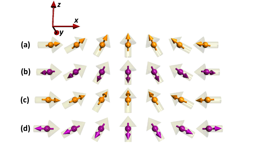
Figure 1: Thick transparent arrows parallel to the $zx$ plane illustrate the magnetization direction in the cycloidal spin spiral of Eq. (43) (for $q<0$). Spheres with attached arrows illustrate conduction electrons and their spins. According to Eq. (60) the spin of a conduction electron has a component in $y$ direction and is therefore not perfectly aligned with the magnetization. (a) Minority electron with $v_{{\bm{k}}nx}<0$: $S_{{\bm{k}}ny}<0$. (b) Majority electron with $v_{{\bm{k}}nx}<0$: $S_{{\bm{k}}ny}>0$. (c) Minority electron with $v_{{\bm{k}}nx}>0$: $S_{{\bm{k}}ny}>0$. (d) Majority electron with $v_{{\bm{k}}nx}>0$: $S_{{\bm{k}}ny}<0$.

We add now the effect of SOI, which is not taken into account in Eq. (42). In non-magnetic crystals with broken inversion symmetry the degeneracy between spin-up and spin-down bands is lifted by SOI, which can be described by an effective ${\bm{k}}$-dependent magnetic field ${\bm{\Omega}}^{\rm SOI}_{{\bm{k}}n}$, which acts on the electron spins (see Refs. Žutić et al. (2004); Winkler (2003); Ganichev and Golub (2014); Manchon et al. (2015) for reviews). This so-called spin-orbit field is an odd function of ${\bm{k}}$ and may be expanded as Ganichev and Golub (2014)

$$\Omega^{\rm SOI}_{{\bm{k}}ni}=\sum_{j}\chi^{(2)}_{nij}k_{j}^{\phantom{1}}+\sum_{jlm}\chi^{(4)}_{nijlm}k_{j}^{\phantom{1}}k_{l}^{\phantom{1}}k_{m}^{\phantom{1}}+\dots,$$ (61)

where $\chi_{nij}^{(2)}$ is the $ij$ element of an axial tensor of second rank, which depends on the band index $n$. $\chi_{nijlm}^{(4)}$ is the $ijlm$ element of an axial tensor of fourth rank.

For the (001) and (111) surfaces of cubic transition metals such as Pt and W symmetry requires that axial second rank tensors be of the form

$${\bm{\chi}}_{n}^{(2)}=\begin{pmatrix}0&\alpha_{n}&0\\ -\alpha_{n}&0&0\\ 0&0&0\\ \end{pmatrix}$$ (62)

if the coordinate frame is chosen such that the surface normal is along $z$ direction. The resulting Zeeman interaction between the spin-orbit field and the electron spin is given by

$$\mu^{\phantom{B}}_{\rm B}{\bm{\sigma}}\cdot{\bm{\Omega}}^{\rm SOI}_{{\bm{k}}n}=\mu^{\phantom{B}}_{\rm B}\alpha^{\phantom{B}}_{n}({\bm{\sigma}}\times{\bm{k}})\cdot\hat{{\bm{e}}}^{\phantom{B}}_{z},$$ (63)

which has the form of the Rashba interaction with a band-dependent Rashba parameter $\alpha^{\phantom{B}}_{n}$.

We now consider magnetic bilayers, where a magnetic layer is deposited on the (001) or (111) surfaces of cubic transition metals, such as Mn/W(001) and Co/Pt(111). When the magnetization is described by the cycloidal spin spiral of Eq. (43), electrons travelling in $x$ direction exhibit non-zero $y$ components of both spin (Eq. (60)) and spin-orbit field:

$$S^{\phantom{k}}_{{\bm{k}}ny} \approx-s^{\phantom{k}}_{{\bm{k}}n}\frac{\hbar^{2}q}{2\Delta\mathcal{E}}\bar{v}^{\phantom{k}}_{{\bm{k}}nx},$$ (64)

$${\bm{\Omega}}_{{\bm{k}}n}^{\rm SOI}\cdot\hat{{\bm{e}}}^{\phantom{y}}_{y} =-\alpha_{n}^{\phantom{n}}k^{\phantom{x}}_{x}.$$

A linear-in-$q$ energy shift results from the Zeeman interaction between $S^{\phantom{k}}_{{\bm{k}}ny}$ and ${\bm{\Omega}}_{{\bm{k}}n}^{\rm SOI}$:

$$\Delta\mathcal{E}_{\rm DMI}^{\rm(I)}\approx\frac{\mu_{\rm B}^{\phantom{D}}\hbar q}{\Delta\mathcal{E}}\int\!\!\frac{{\rm d}^{d}k}{(2\pi)^{d}}\sum_{n}f^{\phantom{D}}_{{\bm{k}}n}\alpha_{n}^{\phantom{n}}k^{\phantom{x}}_{x}s^{\phantom{k}}_{{\bm{k}}n}\bar{v}^{\phantom{k}}_{{\bm{k}}nx}.$$ (65)

We emphasize that the Brillouin zone integral of Eq. (60) is zero because electrons with opposite ${\bm{k}}$ vectors have opposite velocities $\bar{v}^{\phantom{k}}_{{\bm{k}}nx}$ and their $S^{\phantom{k}}_{{\bm{k}}ny}$ cancel. However, $\Delta\mathcal{E}_{\rm DMI}^{\rm(I)}$ is nonzero since both $S^{\phantom{k}}_{{\bm{k}}ny}$ and ${\bm{\Omega}}_{{\bm{k}}n}^{\rm SOI}$ are odd functions of ${\bm{k}}$. Eq. (64) and Eq. (65) are a central result of this section: They show how DMI is related to the spin-orbit field and to the adiabatic spin-transfer torque.

While Eq. (65) provides a useful and intuitive picture of the origin of DMI, it provides only a rather crude estimate because we approximated SOI in the magnetic bilayer by Eq. (63) and we used Eq. (59) to derive the approximation Eq. (60) of $S^{\phantom{k}}_{{\bm{k}}ny}$. In order to obtain a more accurate expression for $\Delta\mathcal{E}_{\rm DMI}^{\rm(I)}$ we use the full spin-orbit interaction $H^{\rm SOI}$ instead of Eq. (65) and we do not use the rigid shift model Eq. (59). This yields:

$$\Delta\mathcal{E}_{\rm DMI}^{\rm(I)}\approx-\frac{\hbar q}{2}\int\!\!\frac{{\rm d}^{d}k}{(2\pi)^{d}}\sum_{n}f_{{\bm{k}}n}\sum_{m\neq n}{\rm Re}\Biggl{\{}$$ (66)

$$\frac{\Bigl{\langle}\bar{u}_{{\bm{k}}n}\Bigl{|}\mathcal{V}_{{\bm{k}}}\Bigr{|}\bar{u}_{{\bm{k}}m}\Bigr{\rangle}\Bigl{\langle}\bar{u}_{{\bm{k}}m}\Bigl{|}\{\sigma_{y},\bar{v}_{x}\}\Bigr{|}\bar{u}_{{\bm{k}}n}\Bigr{\rangle}}{\bar{\mathcal{E}}_{{\bm{k}}n}-\bar{\mathcal{E}}_{{\bm{k}}m}}\Biggr{\}}=$$

$$=qa_{yx}^{\rm(I)}.$$

Here, $a_{yx}^{\rm(I)}$ is the $y$ component of ${\bm{a}}^{\rm(I)}_{x}$, i.e., $a_{yx}=\hat{{\bm{e}}}_{y}\cdot{\bm{a}}^{\rm(I)}_{x}$, where $\hat{{\bm{e}}}_{y}$ is the unit vector in $y$ direction. There are two ways to read this equation. The first way is to consider SOI, i.e., $\mathcal{V}_{{\bm{k}}}$, as perturbation. Then Eq. (66) describes the change of the observable $\hbar\{\sigma_{y},\bar{v}_{x}\}/4$ in response to the perturbation $\mathcal{V}_{{\bm{k}}}$, i.e., it describes part of the SOI-linear contribution to the ground-state spin current. The second way to read Eq. (66) has been described in detail in this section: According to Eq. (49) we can consider $-\hbar q\{\sigma_{y},\bar{v}_{x}\}/4$ as the perturbation arising from the noncollinear spin-spiral structure. Then Eq. (66) describes the response of the observable $\mathcal{V}_{{\bm{k}}}$ to the noncollinear spin-spiral structure. The observable $\mathcal{V}_{{\bm{k}}}$ measures the Zeeman interaction between the spin-orbit field and the noncollinearity-induced spin, i.e., an energy-shift due to DMI. Eq. (66) is a central result of this section: The two ways of reading Eq. (66) explain in a simple and intuitive way why DMI and ground-state spin currents are related.

In the discussion above we considered the special case of flat cycloidal spirals. For a general noncollinear magnetic texture an electron moving with velocity $\bar{{\bm{v}}}_{{\bm{k}}n}$ is misaligned with the local magnetization by

$${\bm{S}}_{{\bm{k}}n} \approx-s_{{\bm{k}}n}\frac{\hbar^{2}}{2\Delta\mathcal{E}}\hat{{\bm{n}}}\times(\bar{{\bm{v}}}_{{\bm{k}}n}\cdot{\bm{\nabla}})\hat{{\bm{n}}}=$$ (67)

$$=-\sum_{j}\bar{v}_{{\bm{k}}nj}s_{{\bm{k}}n}\frac{\hbar^{2}}{2\Delta\mathcal{E}}\left[\hat{{\bm{n}}}\times\frac{\partial\hat{{\bm{n}}}}{\partial r_{j}}\right],$$

which is obtained by generalizing Eq. (60). Assuming that the ${\bm{k}}$-linear term in the spin-orbit field Eq. (61) dominates we can write the energy shift due to the Zeeman interaction of ${\bm{S}}_{{\bm{k}}n}$ with ${\bm{\Omega}}^{\rm SOI}_{{\bm{k}}n}$ as

$$\Delta\mathcal{E}_{\rm DMI}^{\rm(I)}\approx-\frac{\mu_{\rm B}\hbar}{\Delta\mathcal{E}}\int\!\!\frac{{\rm d}^{d}k}{(2\pi)^{d}}\sum_{n}f_{{\bm{k}}n}\times$$ (68)

$$\quad\times\sum_{j}s_{{\bm{k}}n}\bar{v}_{{\bm{k}}nj}\left[{\bm{\chi}}_{n}^{(2)}{\bm{k}}\right]\cdot\left[\hat{{\bm{n}}}\times\frac{\partial\hat{{\bm{n}}}}{\partial r_{j}}\right].$$

Comparing this expression to Eq. (1) leads to the approximation

$${\bm{a}}_{j}^{\rm(I)}\approx-\frac{\mu_{\rm B}\hbar}{\Delta\mathcal{E}}\sum_{n}{\bm{\chi}}_{n}^{(2)}\hat{{\bm{e}}}_{j}\int\!\!\frac{{\rm d}^{d}k}{(2\pi)^{d}}f_{{\bm{k}}n}s_{{\bm{k}}n}\bar{v}_{{\bm{k}}nj}k_{j},$$ (69)

from which it follows that the tensor $a_{ij}^{\rm(I)}$ has the same symmetry properties as the tensors $\chi^{(2)}_{nij}$. This result can also be concluded directly from symmetry arguments, because $D_{ij}=\hat{{\bm{e}}}_{i}\cdot{\bm{D}}_{j}$ is an axial tensor of second rank exactly like $\chi^{(2)}_{ij}$. Thus, $D_{ij}$ is of the form of Eq. (62) for (001) and (111) surfaces of cubic transition metals. Also the torkance tensor that describes the spin-orbit torque is an axial tensor of second rank. Therefore, the symmetry of $D_{ij}$ can be determined from the symmetry of the magnetization-even component of the torkance tensor, which has been determined for all crystallographic point groups Wimmer et al. (2016); Ciccarelli et al. (2016); Železný et al. (2017).

III.2 The contribution ${\bm{a}}_{j}^{\rm(II)}$

In Eq. (49) we describe the perturbation to the Hamiltonian due to the noncollinearity by the anticommutator of the Pauli matrix with the velocity operator $\bar{{\bm{v}}}$, where the effect of SOI is missing in $\bar{{\bm{v}}}$ . In the presence of SOI the term $-\hbar q\{\sigma_{y},v_{x}^{\rm SOI}\}/4$ therefore needs to be added to the perturbation. In the first order this leads to the energy correction described by ${\bm{a}}_{j}^{\rm(II)}$ in Eq. (23).

The SOI-correction of the velocity operator can be written as

$${\bm{v}}^{\rm SOI}=\frac{i}{\hbar}[\mathcal{V}_{{\bm{k}}},{\bm{r}}]=\frac{\mu_{\rm B}}{2mc^{2}e}{\bm{\sigma}}\times{\bm{\nabla}}V,$$ (70)

where we used that SOI is described by the last term in Eq. (7). Eq. (70) allows us to rewrite the anticommutators $\{\sigma_{i},v^{\rm SOI}_{j}\}$ occurring in Eq. (23) as

$$\{\sigma_{i},v^{\rm SOI}_{j}\}=-\frac{\mu_{\rm B}}{mc^{2}e}\epsilon_{ijk}\frac{\partial V({\bm{r}})}{\partial r_{k}},$$ (71)

where we used $\{\sigma_{i},\sigma_{j}\}=2\delta_{ij}$. Finally, we obtain

$$a^{\rm(II)}_{ij} =\hat{{\bm{e}}}_{i}\cdot{\bm{a}}^{\rm(II)}_{j}=$$ (72)

$$=\frac{\hbar\mu_{\rm B}}{4mc^{2}e}\epsilon_{ijk}\int\!\!\frac{{\rm d}^{d}k}{(2\pi)^{d}}\sum_{n}f(\bar{\mathcal{E}}_{{\bm{k}}n})\left\langle\bar{u}_{{\bm{k}}n}\right|\frac{\partial V({\bm{r}})}{\partial r_{k}}\left|\bar{u}_{{\bm{k}}n}\right\rangle,$$

where $\hat{{\bm{e}}}_{i}$ is the unit vector in the $i$-th cartesian direction, $\epsilon_{ijk}$ is the Levi-Civita symbol and $a_{ij}^{\rm(II)}$ is the $i$-th cartesian component of ${\bm{a}}_{j}^{\rm(II)}$. Thus, $a^{\rm(II)}_{ij}$ is directly proportional to the expectation value of the gradient of the scalar effective potential. In centrosymmetric systems this expectation value is zero.

In noncentrosymmetric systems Eq. (72) is generally non-zero, even in non-magnetic systems. However, in non-magnetic systems ${\bm{Q}}_{j}^{(1)}$ has to vanish, because according to Eq. (40) it is related to DMI, which is zero in non-magnetic systems. We therefore prove now that ${\bm{a}}_{j}^{\rm(I)}$ and ${\bm{a}}_{j}^{\rm(II)}$ cancel out in non-magnetic systems. In non-magnetic systems Eq. (22) can be rewritten as

$${\bm{a}}_{yx}^{\rm(I)}= \hat{{\bm{e}}}_{y}\cdot{\bm{a}}_{x}^{\rm(I)}=-\frac{\hbar}{4}{\rm Re}\int\!\!\frac{{\rm d}^{d}k}{(2\pi)^{d}}\sum_{n,m,s}\frac{f(\bar{\mathcal{E}}_{{\bm{k}}ns})-f(\bar{\mathcal{E}}_{{\bm{k}}ms})}{\bar{\mathcal{E}}_{{\bm{k}}ns}-\bar{\mathcal{E}}_{{\bm{k}}ms}}\times$$ (73)

$$\times\langle\bar{u}_{{\bm{k}}ns}|\{\sigma_{y},\bar{v}_{x}\}|\bar{u}_{{\bm{k}}m-s}\rangle\langle\bar{u}_{{\bm{k}}m-s}|\mathcal{V}_{{\bm{k}}}|\bar{u}_{{\bm{k}}ns}\rangle$$

$$=-\frac{\hbar}{2}{\rm Im}\int\!\!\frac{{\rm d}^{d}k}{(2\pi)^{d}}\sum_{n,m,s}s\frac{f(\bar{\mathcal{E}}_{{\bm{k}}ns})-f(\bar{\mathcal{E}}_{{\bm{k}}ms})}{\bar{\mathcal{E}}_{{\bm{k}}ns}-\bar{\mathcal{E}}_{{\bm{k}}ms}}\times$$

$$\times\langle\bar{u}_{{\bm{k}}ns}|\bar{v}_{x}|\bar{u}_{{\bm{k}}ms}\rangle\langle\bar{u}_{{\bm{k}}m-s}|\mathcal{V}_{{\bm{k}}}|\bar{u}_{{\bm{k}}ns}\rangle$$

$$=-\frac{\mu_{\rm B}}{2e\hbar c^{2}}{\rm Re}\int\!\!\frac{{\rm d}^{d}k}{(2\pi)^{d}}\sum_{n,m,s}f(\bar{\mathcal{E}}_{{\bm{k}}ns})\times$$

$$\times\frac{\partial\langle\bar{u}_{{\bm{k}}ns}|}{\partial k_{x}}|\bar{u}_{{\bm{k}}ms}\rangle\langle\bar{u}_{{\bm{k}}ms}|\frac{\partial V({\bm{r}})}{\partial r_{z}}\frac{\partial\bar{H}_{{\bm{k}}}}{\partial k_{x}}|\bar{u}_{{\bm{k}}ns}\rangle$$

$$=\frac{\hbar\mu_{\rm B}}{4emc^{2}}{\rm Re}\int\!\!\frac{{\rm d}^{d}k}{(2\pi)^{d}}\sum_{n,s}f(\bar{\mathcal{E}}_{{\bm{k}}ns})\times$$

$$\times\langle\bar{u}_{{\bm{k}}ns}|\frac{\partial V({\bm{r}})}{\partial r_{z}}|\bar{u}_{{\bm{k}}ns}\rangle.$$

To simplify the equations we treat only the $y$ component of ${\bm{a}}^{\rm(I)}_{x}$ in Eq. (73). The other components can be worked out analogously. $s=\pm 1$ labels the spin, i.e., $s=+1$ denotes spin-up and $s=-1$ denotes spin-down and we used $\langle s|\sigma_{y}|-s\rangle=-is$. Since the system is supposed to be non-magnetic, all energy levels are at least doubly degenerate: $\bar{\mathcal{E}}_{{\bm{k}}n+1}=\bar{\mathcal{E}}_{{\bm{k}}n-1}$. In the last step we have used integration by parts and we have substituted the second $k_{x}$ derivative of $\bar{H}_{{\bm{k}}}$ by $\hbar^{2}/m$. Comparison of Eq. (72) and Eq. (73) shows that $a_{xy}^{\rm(I)}+a_{xy}^{\rm(II)}=0$ in non-magnetic systems (Note that in Eq. (73) the band index $n$ runs over doubly degenerate states and there is an additional spin index $s$. In Eq. (72) there is only one band index, which runs over both spin-up and spin-down states).

IV Interpretation of the ground-state energy current associated with DMI

When the magnetization is time-dependent, e.g., when skyrmions or domain walls are moving or when the magnetization is precessing at the ferromagnetic resonance, a ground-state energy current arises from DMI Freimuth et al. (2016). It is given by

$$\mathscr{J}^{\rm DMI}_{j}=-{\bm{D}}_{j}\cdot\left(\hat{{\bm{n}}}\times\frac{\partial\hat{{\bm{n}}}}{\partial t}\right).$$ (74)

In Eq. (65) we model DMI by the Zeeman interaction between the spin-orbit field and the misalignment of the spins of conduction electrons with the noncollinear magnetic texture. Based on this model we develop an interpretation of the ground-state energy current $\mathscr{J}^{\rm DMI}_{j}$ in the following.

According to Eq. (67) the misalignment of the spin of the electron of band $n$ at $k$ point ${\bm{k}}$ can be written as

$${\bm{S}}_{{\bm{k}}n}({\bm{r}})=\sum_{j}\mathscr{S}^{({\bm{k}}n)}_{j}(\hat{{\bm{n}}}({\bm{r}}))\left(\hat{{\bm{n}}}({\bm{r}})\times\frac{\partial\hat{{\bm{n}}}({\bm{r}})}{\partial r_{j}}\right),$$ (75)

where we introduced the misalignment coefficients $\mathscr{S}^{({\bm{k}}n)}_{j}$, which are given approximately by

$$\mathscr{S}^{({\bm{k}}n)}_{j}\approx-s_{{\bm{k}}n}\frac{\hbar^{2}}{2\Delta\mathcal{E}}\bar{v}_{{\bm{k}}nj}.$$ (76)

We now consider a magnetic texture $\hat{{\bm{n}}}({\bm{r}},t)$ which moves with velocity ${\bm{w}}$ such that

$$\hat{{\bm{n}}}({\bm{r}},t)={\bm{n}}_{0}({\bm{r}}-{\bm{w}}t)$$ (77)

where ${\bm{n}}_{0}({\bm{r}})$ describes for example a domain-wall or a skyrmion at rest. For such a magnetic texture in motion the spin misalignment is time-dependent and satisfies the continuity equation

$$\frac{\partial{\bm{S}}_{{\bm{k}}n}}{\partial t}+\sum_{j}\frac{\partial{\bm{Q}}^{({\bm{k}}n)}_{j}}{\partial r_{j}}=0,$$ (78)

where

$${\bm{Q}}^{({\bm{k}}n)}_{j}=-\mathscr{S}^{({\bm{k}}n)}_{j}(\hat{{\bm{n}}})\left(\hat{{\bm{n}}}\times\frac{\partial\hat{{\bm{n}}}}{\partial t}\right)$$ (79)

is the misaligned part of the spin-current density driven by the motion of the magnetic structure and associated with the electron in band $n$ at $k$-point ${\bm{k}}$.

The Brillouin zone integral of ${\bm{Q}}^{({\bm{k}}n)}_{j}$ is zero:

$$\sum_{n}\int\!\!\frac{{\rm d}^{d}k}{(2\pi)^{d}}f(\bar{\mathcal{E}}_{{\bm{k}}n}){\bm{Q}}^{({\bm{k}}n)}_{j}=0,$$ (80)

because according to Eq. (76) the misalignment coefficients are odd functions of ${\bm{k}}$, i.e., $\mathscr{S}^{(-{\bm{k}}n)}_{j}=-\mathscr{S}^{({\bm{k}}n)}_{j}$, and consequently ${\bm{Q}}^{({\bm{k}}n)}_{j}$ is also an odd function of ${\bm{k}}$, i.e., ${\bm{Q}}^{(-{\bm{k}}n)}_{j}=-{\bm{Q}}^{({\bm{k}}n)}_{j}$. Consequently, Eq. (79) does not lead to a net spin current, but it describes counter-propagating spin-currents, where the spin-current carried by electrons at $k$-point ${\bm{k}}$ has the opposite sign of the spin-current carried by electrons at $-{\bm{k}}$.

From Eq. (75) until Eq. (80) SOI is not yet considered. Therefore, the ground-state spin current associated with SOI is not present. However, even in the absence of SOI, there are several additional spin currents present that are not included in our definition of ${\bm{Q}}^{({\bm{k}}n)}_{j}$. First, there is the spin current

$${\bm{Q}}^{\rm xc}_{j}=\sum_{n}\int\!\!\frac{{\rm d}^{d}k}{(2\pi)^{d}}f(\bar{\mathcal{E}}_{{\bm{k}}n}){\bm{S}}_{{\bm{k}}n}\bar{v}_{{\bm{k}}nj},$$ (81)

which mediates the exchange-stiffness torque. In contrast to ${\bm{Q}}^{({\bm{k}}n)}_{j}$ the spin current ${\bm{Q}}^{\rm xc}_{j}$ is zero in collinear systems, i.e, whenever $\partial\hat{{\bm{n}}}/\partial{\bm{r}}=0$. However, the Brillouin-zone integration leads to a nonzero value of ${\bm{Q}}^{\rm xc}_{j}$ in noncollinear systems, while the Brillouin-zone integral of ${\bm{Q}}^{({\bm{k}}n)}_{j}$ vanishes according to Eq. (80). Second, the time-dependence of $\hat{{\bm{n}}}$ can lead to spin-pumping, in particular in magnetic bilayer systems. Most discussions on spin-pumping focus on net spin currents (by ’net’ we mean that in contrast to Eq. (80) the Brillouin zone integral is not zero) that flow in magnetic bilayer systems from the magnet into the nonmagnet. In contrast, the spin currents described by Eq. (79) are counter-propagating, i.e., ${\bm{Q}}^{(-{\bm{k}}n)}_{j}=-{\bm{Q}}^{({\bm{k}}n)}_{j}$. However, in analogy to the discussion of Eq. (64), we will show now that such counter-propagating spin currents are exactly what is needed to interpret the ground-state energy current $\mathscr{J}^{\rm DMI}_{j}$.

In order to include SOI, we multiply Eq. (78) by the spin-orbit field. Subsequently, we integrate over the Brillouin zone and add the contributions of all occupied bands. This yields the continuity equation for DMI energy

$$\frac{\partial(\Delta\mathcal{E}^{\rm(I)}_{\rm DMI})}{\partial t}+\sum_{j}\frac{\partial\mathscr{J}_{j}^{\rm DMI,I}}{\partial r_{j}}=0,$$ (82)

where

$$\mathscr{J}_{j}^{\rm DMI,I}=\frac{2\mu_{\rm B}}{\hbar}\sum_{n}\int\!\!\frac{{\rm d}^{d}k}{(2\pi)^{d}}f(\bar{\mathcal{E}}_{{\bm{k}}n}){\bm{Q}}^{({\bm{k}}n)}_{j}\cdot{\bm{\Omega}}_{{\bm{k}}n}^{\rm SOI}$$ (83)

is a ground-state energy current associated with DMI. This approximation leads to the picture that $\mathscr{J}_{j}^{\rm DMI,I}$ is associated with counter-propagating spin currents, where the spins carry energy due to their Zeeman interaction with the spin-orbit field. Since both ${\bm{Q}}^{({\bm{k}}n)}_{j}$ and ${\bm{\Omega}}_{{\bm{k}}n}^{\rm SOI}$ are odd functions of ${\bm{k}}$, $\mathscr{J}_{j}^{\rm DMI,I}$ is nonzero in systems with inversion asymmetry.

The continuity equation of DMI energy, Eq. (82), has been discussed in detail in Ref. Freimuth et al. (2016). It describes that DMI energy associated with domain walls or skyrmions in motion moves together with these objects. In this section we have shown that Eq. (82) results from the continuity equation, Eq. (78), of the spin misalignment.

V Rashba model

We consider the model Hamiltonian

$$H_{{\bm{k}}}=\frac{\hbar^{2}}{2m}k^{2}+\alpha({\bm{k}}\times\hat{{\bm{e}}}_{z})\cdot{\bm{\sigma}}+\frac{\Delta V}{2}\sigma_{z},$$ (84)

where the first term is the kinetic energy, the second term describes the Rashba spin-orbit coupling and the third term describes the exchange interaction. The velocity operators are given by the expressions Sinova et al. (2004)

$$v_{x} =\frac{\hbar}{m}k_{x}-\frac{\alpha}{\hbar}\sigma_{y}$$ (85)

$$v_{y} =\frac{\hbar}{m}k_{y}+\frac{\alpha}{\hbar}\sigma_{x}$$

and the spin velocity operators are Inoue et al. (2004)

$$\frac{\hbar}{4}\{v_{y},\sigma_{x}\}=\frac{\hbar^{2}}{2m}k_{y}\sigma_{x}+\frac{1}{2}\alpha$$ (86)

$$\frac{\hbar}{4}\{v_{x},\sigma_{y}\}=\frac{\hbar^{2}}{2m}k_{x}\sigma_{y}-\frac{1}{2}\alpha.$$

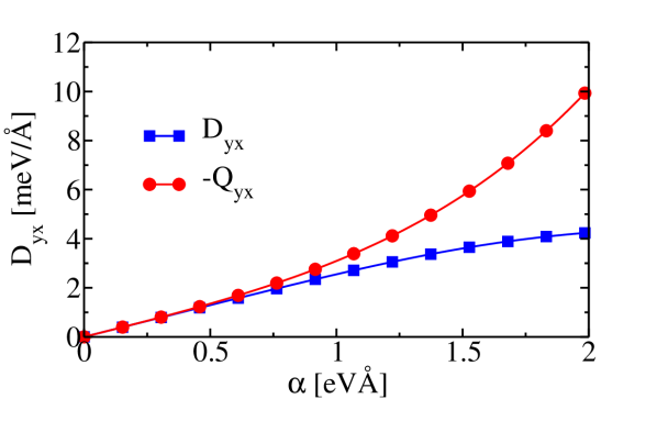
Figure 2: DMI coefficient $D_{yx}$ (squares) and spin current $Q_{yx}$ (circles) vs. $\alpha$ in the Rashba model Eq. (84) for the parameters $\mu=0$ and $\Delta V=$1eV.

First, we discuss the case $\Delta V=0$, where DMI vanishes. For the ground-state spin currents, Eq. (5), the following analytical expressions are readily derived

$${\bm{Q}}_{x}=-\frac{m^{2}\alpha^{3}}{6\pi\hbar^{4}}\hat{{\bm{e}}}_{y},$$ (87)

$${\bm{Q}}_{y}=\frac{m^{2}\alpha^{3}}{6\pi\hbar^{4}}\hat{{\bm{e}}}_{x},$$

when the temperature $T=0$ and when the chemical potential $\mu>0$. In agreement with our discussion in section III.2 there is no $\alpha$-linear term in Eq. (87) because the system is nonmagnetic due to $\Delta V=0$. On the other hand, the ground-state spin currents are nonzero even in this nonmagnetic case. Since DMI vanishes for nonmagnetic systems Eq. (6) is violated, while Eq. (40) is fulfilled.

Next, we discuss the magnetic case. Figure 2 shows the DMI-coefficient $D_{yx}$ and the ground-state spin current $Q_{yx}$ for $\Delta V=$1eV at $\mu=0$ as a function of $\alpha$. In the SOI-linear regime, i.e., for small $\alpha$, we find $D_{yx}=-Q_{yx}$, in agreement with the analytical result in Eq. (40). For large values of $\alpha$ nonlinearities become pronounced in both $D_{yx}$ and $Q_{yx}$. Interestingly, $Q_{yx}$ exhibits stronger nonlinearity than $D_{yx}$ does. Therefore, also in the magnetic Rashba model Eq. (6) is violated, while Eq. (40) is fulfilled.

VI Ab-initio calculations

In the following we discuss DMI and ground-state spin currents in Mn/W(001) and Co/Pt(111) magnetic bilayers based on ab-initio density-functional theory calculations. The Mn/W(001) system consists of one monolayer of Mn deposited on 9 layers of W(001) in our simulations. The Co/Pt(111) bilayer is composed of 3 layers of Co deposited on 10 layers of Pt(111). Computational details of the electronic structure calculations are given in Ref. Freimuth et al. (2014a), where we investigated spin-orbit torques in Mn/W(001) and Co/Pt(111). We use Eq. (5) to evaluate the full ground-state spin-current density $Q_{yx}=\hat{{\bm{e}}}_{y}\cdot{\bm{Q}}_{x}$. Its SOI-linear part $Q^{(1)}_{yx}=-a_{yx}^{\rm(I)}-a_{yx}^{\rm(II)}$ is calculated from Eq. (22) and from Eq. (23). We employ Eq. (2) to compute the DMI coefficient $D_{yx}=\hat{{\bm{e}}}_{y}\cdot{\bm{D}}_{x}$. The temperature in the Fermi function $f(\mathcal{E})$ and in the grand canonical potential density $g(\mathcal{E})$ is set to $T=300$K.

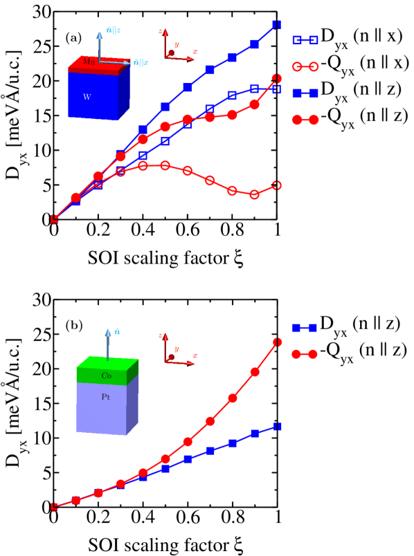
Figure 3: DMI coefficient $D_{yx}$ (squares) and spin current $Q_{yx}$ (circles) vs. SOI scaling factor $\xi$ in (a) Mn/W(001) and (b) Co/Pt(111). For the Mn/W(001) magnetic bilayer results are shown for magnetization along $z$ ($\hat{{\bm{n}}}\|z$) and for magnetization along $x$ ($\hat{{\bm{n}}}\|x$). For the Co/Pt(111) magnetic bilayer results are shown for magnetization along $z$. The insets illustrate the geometry and the coordinate system.

In Figure 3 we plot both the spin current $Q_{yx}=\hat{{\bm{e}}}_{y}\cdot{\bm{Q}}_{x}$ and the DMI coefficient $D_{yx}=\hat{{\bm{e}}}_{y}\cdot{\bm{D}}_{x}$ as a function of SOI scaling factor $\xi$ for the two systems Mn/W(001) and Co/Pt(111). The figure shows that in the linear regime, i.e., for small $\xi$, the relation $D_{yx}=-Q_{yx}$ is satisfied very well, in agreement with the analytical result in Eq. (40). For large values of $\xi$ nonlinear contributions become important for both $Q_{yx}$ and $D_{yx}$ and the DMI coefficient is no longer described very well by the ground-state spin current.

In Mn/W(001) we show $Q_{yx}$ and $D_{yx}$ for two different magnetization directions $\hat{{\bm{n}}}$, namely $\hat{{\bm{n}}}\|z$ and $\hat{{\bm{n}}}\|x$. Both $Q_{yx}$ and $D_{yx}$ depend on $\hat{{\bm{n}}}$. For small $\xi$ the $\hat{{\bm{n}}}$-dependence of $D_{yx}$ is well described by the $\hat{{\bm{n}}}$-dependence of $Q_{yx}$. However, at $\xi=1$ the $\hat{{\bm{n}}}$-dependence of $Q_{yx}$ is much stronger than the $\hat{{\bm{n}}}$-dependence of $D_{yx}$.

Interestingly, $Q_{yx}$ is much more nonlinear in $\xi$ than $D_{yx}$ in the considered $\xi$ range. This leads to large deviations between $D_{yx}$ and $-Q_{yx}$ at $\xi=1$. Since $D_{yx}$ is almost linear up to $\xi=1$, a good approximation is $D_{yx}\approx-Q^{(1)}_{yx}$. This is a major difference to the B20 compounds Mn_1-xFe_xGe and Fe_1-xCo_xGe for which $D_{yx}\approx-Q_{yx}$ has been found to be a good approximation Kikuchi et al. (2016). Due to the strong SOI from the 5$d$ heavy metals in the magnetic bilayer systems considered in this work the SOI-nonlinear contributions in $Q_{yx}$ require to extract the SOI-linear part $Q^{(1)}_{yx}$ in order to approximate DMI by the spin current as $D_{yx}\approx-Q^{(1)}_{yx}$.

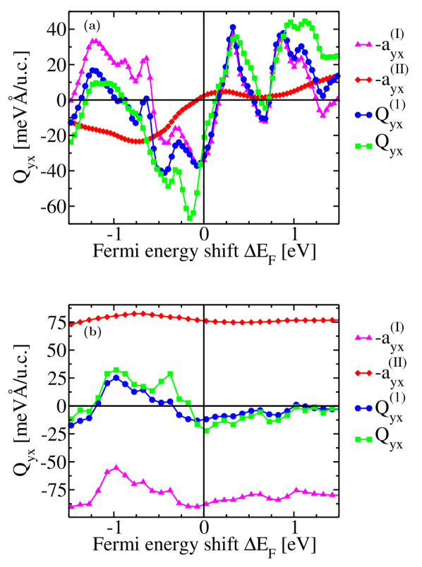
Figure 4: Spin current $Q_{yx}$ (squares), SOI linear contribution $Q^{(1)}_{yx}$ to the spin current (circles), and the contributions $a_{yx}^{\rm(I)}$ (triangles) and $a_{yx}^{\rm(II)}$ (diamonds) to $Q^{(1)}_{yx}=-a_{yx}^{\rm(I)}-a_{yx}^{\rm(II)}$. Results are shown as a function of Fermi energy shift $\Delta E_{\rm F}$ in (a) Mn/W(001) and (b) Co/Pt(111) for magnetization in $z$ direction.

The finding that $D_{yx}\approx-Q^{(1)}_{yx}$ is a good approximation despite the strong SOI from the heavy metals motivates us to investigate $Q^{(1)}_{yx}$ further by splitting it up into its two contributions $-a_{yx}^{\rm(I)}$ and $-a_{yx}^{\rm(II)}$. In Figure 4 we show $Q^{(1)}_{yx}$ and the two contributions $-a_{yx}^{\rm(I)}$ and $-a_{yx}^{\rm(II)}$. In order to investigate chemical trends we artificially shift the Fermi level by $\Delta E_{\rm F}$. The Mn/W and Co/Pt bilayer systems correspond to $\Delta E_{\rm F}=0$. Negative values of $\Delta E_{\rm F}$ approximately describe the doped systems Mn_1-xCr_x/W_1-xTa_x and Co_1-xFe_x/Pt_1-xIr_x, while positive values of $\Delta E_{\rm F}$ approximately describe the doped systems Mn_1-xFe_x/W_1-xRe_x and Co_1-xNi_x/Pt_1-xAu_x. Figure 4 clearly shows that $a_{yx}^{\rm(I)}$ and $a_{yx}^{\rm(II)}$ are generally of similar magnitude. In Mn/W(001) at $\Delta E_{\rm F}=0$ there is a crossing of ${\bm{a}}_{yx}^{\rm(II)}$ through zero and therefore $Q^{(1)}_{yx}\approx-a_{yx}^{\rm(I)}$. However, for $\Delta E_{\rm F}\neq 0$ both $a_{yx}^{\rm(I)}$ and $a_{yx}^{\rm(II)}$ are important. In Co/Pt(111) both $a_{yx}^{\rm(I)}$ and $a_{yx}^{\rm(II)}$ are much larger in magnitude than $Q^{(1)}_{yx}$ but opposite in sign. We also show $Q_{yx}$ in Figure 4. $Q_{yx}$ and $Q^{(1)}_{yx}$ behave similarly as a function of $\Delta E_{\rm F}$. However, due to the strong SOI from the 5$d$ transition metal, $Q_{yx}$ and $Q^{(1)}_{yx}$ often deviate substantially.

Figure 5: DMI coefficient $D_{yx}$ (squares) and the part $a_{yx}^{\rm(I,4)}$ of $a_{yx}^{\rm(I)}$ where SOI is switched-off in all Pt layers that are far away from the Co/Pt interface (triangles). Results are shown as a function of Fermi energy shift $\Delta E_{\rm F}$ in Co/Pt(111) for magnetization in $z$ direction.

Numerical tests in Fe and Ni have shown that the effect of the SOI-correction $v^{\rm SOI}_{j}$ on optical conductivities and the magneto-optical Kerr effect is small Wang and Callaway (1974); Li et al. (2007). At first glance, it is therefore surprising that $a_{yx}^{\rm(II)}$ is as important as $a_{yx}^{\rm(I)}$ in Co/Pt(111) according to Fig. 4. One reason is that SOI in Pt is stronger than in Fe and Ni, but a second important reason is that from the 10 layers of Pt only the first few layers close to the interface matter for DMI while all Pt layers contribute to $a_{yx}^{\rm(I)}$ and to $a_{yx}^{\rm(II)}$. In order to illustrate this we calculate the coefficient $a_{yx}^{\rm(I,4)}$, which is obtained from Eq. (22) when SOI is included only in the 3 Co layers and in the adjacent interfacial Pt layer and artificially switched off in the other 9 Pt layers. We plot the resulting coefficient $a_{yx}^{\rm(I,4)}$ in Fig. 5 as a function of Fermi energy shift $\Delta E_{\rm F}$ and compare it to the DMI coefficient $D_{yx}$. Fig. 5 shows that $a_{yx}^{\rm(I,4)}$ is a good approximation for $D_{yx}$ in the region -0.75 eV$<\Delta E_{\rm F}<$0. This suggests the picture that the essential DMI physics in transition metal bilayers is contained in $a_{yx}^{\rm(I)}$. However, when the 5$d$ heavy metal layer is very thick, $a_{yx}^{\rm(I)}$ gets contaminated by $-a_{yx}^{\rm(II)}$ and therefore the correct expression in first order of SOI is $D_{yx}^{\rm(1)}=a_{yx}^{\rm(I)}+a_{yx}^{\rm(II)}$. This interpretation is also in line with our discussion in Section III.2, where we point out that $a_{yx}^{\rm(I)}$ and $a_{yx}^{\rm(II)}$ may individually be nonzero in nonmagnets while their sum cancels out in nonmagnets.

VII Summary and Outlook

We show analytically that at the first order in the perturbation by SOI DMI is given by the ground-state spin current. As a consequence, ground-state spin currents in nonmagnetic systems cannot exist at the first order in SOI. In the special case of the Rashba model they arise at the third order in SOI. This clarifies the connection between the Berry-phase approach and the spin-current approach to DMI. The SOI-linear contribution to DMI can be decomposed into two contributions. The first contribution can be understood by mapping spin-spirals onto magnetically collinear systems by a gauge transformation and adding spin-orbit coupling perturbatively. We obtain an intuitive interpretation of the first contribution as Zeeman interaction between the spin-orbit field and the misalignment of electron spins in magnetically noncollinear textures. We discuss how the misalignment is related to the spin-transfer torque and how the symmetry of DMI is related to the spin-orbit field. Thereby, we also provide a simple explanation why DMI and the ground-state spin current are related. The second contribution arises from the SOI-correction to the velocity operator. While the SOI-correction to the velocity operator is in principle small in transition metals, its contribution to DMI cannot be neglected in magnetic bilayer systems with thick heavy metal layers. When magnetic textures are moving, the spin misalignment of electrons leads to counter-propagating spin currents. These counter-propagating spin currents carry energy due to their Zeeman interaction with the spin-orbit field. Thereby, our theory highlights the connections of DMI to spintronics concepts such as spin-orbit fields and spin-transfer torque. We calculate DMI and ground-state spin currents from ab-initio in Mn/W(001) and Co/Pt(111) magnetic bilayers. We find that due to the strong SOI from the heavy metal layers DMI is not well approximated by the full ground-state spin current. Thereby, we illustrate the limitations of the spin-current approach to DMI in systems with strong SOI. However, the SOI-linear contribution to the ground-state spin current provides a good and useful approximation for DMI in systems with strong SOI because DMI is much more linear in SOI than the ground-state spin current is.

The application of electric fields or light can change the DMI coefficients Mikhaylovskiy et al. (2015). While a complete ab-initio theory of nonequilibrium exchange interactions and DMI is still missing, an interesting application of the spin-current description of DMI is the estimation of the variation of DMI by nonequilibrium spin currents excited by applied electric fields or by light. In order to induce or to modify DMI the spin in the nonequilibrium spin current needs to have a component perpendicular to the magnetization. One option to generate such a spin current is the spin Hall effect Sinova et al. (2015), which allows the generation of spin currents of the order of $10^{7}$A/cm${}^{2}\hbar/e$ in metals with large SOI. A spin current of this size corresponds to a DMI-change of the order of 0.05 meVÅ  per atom. While this is smaller than the equilibrium DMI in Mn/W and Co/Pt by more than 2 orders of magnitude and therefore difficult to measure in these systems, DMI-changes due to the spin Hall effect might be measurable in systems with small or zero DMI. Using femtosecond laser pulses one can excite significantly stronger nonequilibrium spin currents of the order of $10^{9}$A/cm${}^{2}\hbar/e$ Kampfrath et al. (2013). For such strong spin-currents the spin-current picture of DMI leads to the estimate of a DMI-change of 5 meVÅ  per atom, which is the order of magnitude of the equilibrium DMI in Mn/W and Co/Pt bilayer systems.