Influence of the vector interaction and an external magnetic field on the isentropes near the chiral critical end point

Abstract

The location of the critical end point (CEP) and the isentropic trajectories in the QCD phase diagram are investigated. We use the (2+1) Nambu$-$Jona-Lasinio model with the Polyakov loop coupling for different scenarios, namely by imposing zero strange quark density, which is the case in the ultra relativistic heavy-ion collisions, and $\beta$-equilibrium. The influence of strong magnetic fields and of the vector interaction on the isentropic trajectories around the CEP is discussed. It is shown that the vector interaction and the magnetic field, having opposite effects on the first-order transition, affect the isentropic trajectories differently: as the vector interaction increases, the first-order transition becomes weaker and the isentropes become smoother; when a strong magnetic field is considered, the first-order transition is strengthened and the isentropes are pushed to higher temperatures. No focusing of isentropes in region towards the CEP is seen.

I Introduction

The main goal of the heavy-ion collision (HIC) program is to understand strong force and extended systems governed by Quantum Chromodynamics (QCD). Developments over the last two decades allowed the creation and investigation of new forms of QCD matter characterized by high parton densities. One major achievement in HIC was the discovery that QCD matter at energy densities greater than 1 GeV/fm³ acts like a strongly interacting plasma of quarks and gluons. Indeed, the fast (local) thermalization time and the good agreement of the data at RHIC with ideal relativistic hydrodynamics models (which admit a fluid evolution with zero viscosity) are evidences that the matter formed at RHIC is a strongly interacting plasma of quarks and gluons d'Enterria:2006su , as confirmed by the Large Hadron Collider (LHC) data Averbeck:2015jja .

Since in HIC the expansion of the quark-gluon plasma (QGP) is accepted to be a hydrodynamic expansion of an ideal fluid, it will nearly follow trajectories of constant entropy, the so-called isentropes. Due to the conservation of the baryon number, the isentropic trajectories are lines of constant entropy per baryon ($s/\rho_{B}$) in the ($T,\mu_{B}$) space with zero strange quark density, $\rho_{s}=0$, which contain important information on the adiabatic evolution of the system. For AGS, SPS, and RHIC the values of $s/\rho_{B}$ are 30, 45, and 300, respectively Bluhm:2007nu . Lattice results for the isentropic (2+1) flavors equation of state (EOS) at these values of $s/\rho_{B}$ are given in Refs. DeTar:2010xm ; Borsanyi:2012cr .

In Ref. Asakawa:2008ti it was proposed that the presence of a critical end point (CEP) in the QCD phase diagram deforms the trajectories describing the evolution of the expanding fireball. This will have important consequences on the search for the CEP, because modifications of the expansion trajectory may lead to observable effects in the hadron spectra (see Ref. Senger:2011zza ).

The possible existence of the CEP and its implications to the QCD phase diagram is a very timely topic that has drawn the attention of the physics community. From the theoretical point of view, the location of the CEP has been intensively investigated by using lattice QCD calculations (despite the fermion sign problem, extrapolation methods have been used to access the region of small chemical potentials and look for the CEP Endrodi:2011gv ), and more recently by using Dyson-Schwinger equations Fischer:2014ata . Also, effective models such as the Nambu$-$Jona-Lasinio (NJL) model and its extensions, like the NJL model with eight-quark interactions and the Polyakov$-$Nambu$-$Jona-Lasinio (PNJL) model, have been used to study critical properties around the CEP Costa:2008yh ; Hiller:2008nu ; Costa:2008gr .

From the experimental point of view, the location of the CEP is one major goal of several HIC programs, but so far, no definitive results have been found about its location, and even its existence remains a mystery. Since 2010, the Beam Energy Scan (BES-I) program at RHIC has been searching for the experimental signatures of the first-order phase transition and the CEP by colliding Au ions at several energies Abelev:2009bw . In the near future it is expected that, if the CEP exists at a baryonic chemical potential below 400 MeV, the upcoming BES-II program can provide data on fluctuation and flow observables which should yield quantitative evidence for the presence of the CEP. Also, at RHIC, the STAR Collaboration is looking for the CEP, but no definitive conclusions were possible from their measurements of the moments of net-charge multiplicity distributions. Future measurements with high statistics data will be needed Adamczyk:2014fia .

The NA49 program at CERN SPS has also investigated the CEP’s location in nuclear collisions at 158$A$ GeV by analyzing $\pi^{+}\pi^{-}$ pairs with an invariant mass very close to the two-pion threshold, looking for critical fluctuations of the sigma component in a hadronic medium Anticic:2009pe . Sizable effects of $\pi^{+}\pi^{-}$ pair fluctuations with critical characteristics were found in Si + Si collisions, but these effects could not be directly related to the presence of the CEP. Presently, the NA61/SHINE program is dedicated to looking for the CEP and investigating the properties of the onset of deconfinement in light and heavy ion collisions Gazdzicki:2011fx ; Aduszkiewicz:2015jna .

Recently, new possible hints on the CEP were given:

• in Lacey:2014wqa a finite-size scaling analysis of non-monotonic excitation functions for the Gaussian emission source radii difference obtained from two-pion interferometry measurements in Au+Au ($\sqrt{s_{NN}}=7.7-200$ GeV) and Pb+Pb ($\sqrt{s_{NN}}=2.76$ TeV) collisions suggests a second order phase transition with the estimated location of the CEP at $T^{\,CEP}=165$ MeV and $\mu_{B}^{CEP}=95$ MeV;

• in Bugaev:2014bua it was observed a sharp peak in the trace-anomaly and a local minimum of the generalized specific volume at a laboratory energy of 11.6 AGeV which can provide a signal for the formation of a mixed phase between the quark-gluon plasma and the hadron phase;

• in Nara:2016phs it is argued that the observed collapse of directed flow of protons and pions at mid-rapidity at 9 GeV $<\sqrt{s_{NN}}<20$ GeV is the evidence for the softening of the QCD equation of state (EoS), possibly caused by a first-order phase transition.

If these results are confirmed, i.e., an unambiguous experimental identification of a first-order phase transition from the hadronic phase to the deconfined phase, and having in mind that lattice QCD calculations at zero baryon chemical potential show an analytic crossover for the transition from hadrons to quarks and gluons Aoki:2006we ; Aoki:2009sc ; Borsanyi:2013bia , the existence of the CEP gains a strong foothold.

As a matter of fact, it might be easier to detect the first-order phase-coexistence region than the CEP: when the expanding matter created in a HIC eventually crosses a first-order phase transition line the system probably will spend sufficient time in this region to develop measurable signals. Possible observables of this transition are based on the clumping of the system due to spinodal phase decomposition. This could lead to enhanced fluctuations of observables like the strangeness: the enhancement of the kaon-to-pion fluctuations can be the result of the enhancement of fluctuations in the strangeness sector (for a review, see Ref. Senger:2011zza ). These fluctuations caused by spinodal instabilities are a generic phenomenon of first-order phase transitions and may be less suppressed by the short lifetime and the finite size of the system, as compared to critical fluctuations needed to detect the CEP.

The experience acquired in theoretical and experimental investigations concerning the nuclear liquid-gas phase transition can be very useful to the study of deconfinement and chiral phase transitions in relativistic HIC Mishustin:2006ka . Indeed, in Ref. Borderie:2001jg , the spinodal instabilities as a signal of the nuclear liquid-gas phase transition have been successfully identified in nuclear multifragmentation.

In the next several years, planned experiments at FAIR (GSI) and at NICA (JINR) will strengthen the search for the CEP (and the first-order transition of the QCD phase diagram) by exploring regions of higher baryonic chemical potentials, and definitive conclusions concerning its possible existence and location are expected (a review on the experimental search of the CEP can be found in Ref. Akiba:2015jwa ).

It is also important to point out that the location of the CEP is affected by several conditions like the isospin or strangeness content of the medium Costa:2013zca , the role of the vector interaction in the medium Fukushima:2008wg ; Costa:2015bza or the presence of an external magnetic field Costa:2013zca ; Costa:2015bza . The possible location of the CEP will allow us to set stricter constraints on effective models.

Considering all that has been mentioned above, together with its relevance for the understanding of the QCD phase diagram, in the present work we investigate the isentropic trajectories crossing the chiral phase transition around the CEP in both the crossover and first-order transition regions. We consider different scenarios of interest for the phase diagram obtained by choosing different values of the isospin and the strangeness chemical potentials. Finally, we explore the effects of the vector interaction and of an external magnetic field on the isentropic trajectories around the CEP.

II Model and Formalism

To investigate quark matter subject to strong magnetic fields, we will use the PNJL model Fukushima:2003fw ; Ratti:2005jh with 2+1 flavors and a vector interaction. The PNJL Lagrangian in the presence of an external magnetic field is given by

$${\cal L} ={\bar{\psi}}\left[i\gamma_{\mu}D^{\mu}-{\hat{m}}_{f}\right]\psi+G_{S}\sum_{a=0}^{8}\left[({\bar{\psi}}\lambda_{a}\psi)^{2}+({\bar{\psi}}i\gamma_{5}\lambda_{a}\psi)^{2}\right]$$

$$-G_{D}\left\{{\rm det}\left[{\bar{\psi}}(1+\gamma_{5})\psi\right]+{\rm det}\left[{\bar{\psi}}(1-\gamma_{5})\psi\right]\right\}$$

$$-G_{V}\sum_{a=0}^{8}\left[({\bar{\psi}}\gamma^{\mu}\lambda_{a}\psi)^{2}+({\bar{\psi}}\gamma^{\mu}\gamma_{5}\lambda_{a}\psi)^{2}\right]$$

$$+\mathcal{U}\left(\Phi,\bar{\Phi};T\right)-\frac{1}{4}F_{\mu\nu}F^{\mu\nu}$$ (1)

The quark sector is described by the SU(3) version of the NJL model where $G_{S}$ represents the four-Fermi coupling constant and $G_{D}$ denotes the ’t Hooft interaction strength Klevansky:1992qe ; Hatsuda:1994pi ; Buballa:2003qv .

In Eq. (1), $\psi=(u,d,s)^{T}$ is the quark field with three flavors, and ${\hat{m}}_{f}={\rm diag}_{f}(m_{u},m_{d},m_{s})$ is the corresponding (current) mass matrix. $\lambda_{0}=\sqrt{2/3}I$, where $I$ is the unit matrix in the three-flavor space, and $0<\lambda_{a}\leq 8$ denote the Gell-Mann matrices.

The coupling between the (electro)magnetic field $B$ and quarks, and that between the effective gluon field and quarks, is implemented via the covariant derivative $D^{\mu}=\partial^{\mu}-iq_{f}A_{EM}^{\mu}-iA^{\mu}$, where $q_{f}$ is the quark electric charge ($q_{d}=q_{s}=-q_{u}/2=-e/3$), $A^{EM}_{\mu}$ and $F_{\mu\nu}=\partial_{\mu}A^{EM}_{\nu}-\partial_{\nu}A^{EM}_{\mu}$ are used to account for the external magnetic field, and $A^{\mu}(x)=g_{strong}{\cal A}^{\mu}_{a}(x)\frac{\lambda_{a}}{2}$, where ${\cal A}^{\mu}_{a}$ is the SU${}_{c}(3)$ gauge field. A static and constant magnetic field in the $z$ direction, $A^{EM}_{\mu}=\delta_{\mu 2}x_{1}B$, is considered. In the Polyakov gauge, $A^{\mu}=\delta^{\mu}_{0}A^{0}$, with $A^{0}=-iA_{4}$. The trace of the Polyakov line defined by $\Phi=\frac{1}{N_{c}}{\langle\langle\mathcal{P}\exp i\int_{0}^{\beta}d\tau\,A_{4}\left(\vec{x},\tau\right)\ \rangle\rangle}_{\beta}$ is the Polyakov loop which is the exact order parameter of the $\mathbb{Z}_{3}$ symmetric/broken phase transition in pure gauge.

To describe the pure gauge sector, we choose an effective potential, $\mathcal{U}\left(\Phi,\bar{\Phi};T\right)$, which allows us to reproduce the results obtained in lattice calculations Roessner:2006xn :

$$\frac{\mathcal{U}\left(\Phi,\bar{\Phi};T\right)}{T^{4}} =-\frac{a\left(T\right)}{2}\bar{\Phi}\Phi$$

$$+b(T)\mbox{ln}\left[1-6\bar{\Phi}\Phi+4(\bar{\Phi}^{3}+\Phi^{3})-3(\bar{\Phi}\Phi)^{2}\right],$$

where $a\left(T\right)=a_{0}+a_{1}\left(\frac{T_{0}}{T}\right)+a_{2}\left(\frac{T_{0}}{T}\right)^{2}$, $b(T)=b_{3}\left(\frac{T_{0}}{T}\right)^{3}$. The choice of the parameters for the effective potential $\mathcal{U}\left(\Phi,\bar{\Phi};T\right)$ is $a_{0}=3.51$, $a_{1}=-2.47$, $a_{2}=15.2$, and $b_{3}=-1.75$. The parameter $T_{0}$ of the Polyakov potential defines the onset of deconfinement and is fixed to $270$ MeV according to the critical temperature for the deconfinement in pure gauge lattice findings Kaczmarek:2002mc . This potential was constructed in order to describe, for the pure Yang-Mills sector, the expectation value of the color traced Polyakov loop (which acts as an order parameter for the confinement-deconfinement transition). Other potentials were proposed in literature (see for example Ref. Fukushima:2008wg ). However, a new and consistent Polyakov-loop potential fitted to the latest lattice data that are continuum extrapolated and cover a large temperature range is needed. This new effective potential will eventually change the behavior of the isentropic trajectories. Since this new potential is not yet available, we utilize the potential most commonly used in the literature given by Eq. (LABEL:Ueff).

The thermodynamical potential $\Omega$ is written as

$$\Omega(T,\mu,B) =2G_{S}\sum_{f=u,d,s}\left\langle\bar{\psi}_{f}\psi_{f}\right\rangle^{2}-4G_{D}\left\langle\bar{\psi}_{u}\psi_{u}\right\rangle$$

$$\times\left\langle\bar{\psi}_{d}\psi_{d}\right\rangle\left\langle\bar{\psi}_{s}\psi_{s}\right\rangle-2G_{V}\sum_{f=u,d,s}\left\langle\psi^{\dagger}_{f}\psi_{f}\right\rangle^{2}$$

$$+\sum_{f=u,d,s}\left(\Omega_{\text{vac}}^{f}+\Omega_{\text{med}}^{f}+\Omega_{\text{mag}}^{f}\right)+{\cal U}(\Phi,\bar{\Phi},T)$$ (3)

where $\Omega_{\text{vac}}^{f}$, $\Omega_{\text{med}}^{f}$, and $\Omega_{\text{mag}}^{f}$ are the flavor contributions from the vacuum, medium and magnetic field, respectively, which can be found in the Appendix A. The effective chemical potential, for each flavor, is given by

$$\tilde{\mu}_{f}=\mu_{f}-4G_{V}\rho_{f},\,\,\,\,f=u,d,s.$$ (4)

The equation of state for the entropy density, $s$, is given by

$$s(T,\mu,B)=-\frac{\partial\Omega}{\partial T}.$$ (5)

Since the model is not renormalizable, we regularize it by using a sharp cutoff in 3-momentum space, $\Lambda$, for the divergent ultraviolet integrals only. For our numerical calculations we adopt the parameter set obtained in Ref. Rehberg:1995kh : $\Lambda=602.3$ MeV, $G_{S}\Lambda^{2}=1.835$, $G_{D}\Lambda^{5}=12.36$, $m_{u}=m_{d}=5.5$ MeV, $m_{s}=140.7$ MeV. In the vacuum ($T=\mu_{q}=0$), this choice of parameters gives the quark masses $M^{vac}_{q}=M^{vac}_{u}=M^{vac}_{d}=367.7$ MeV and $M^{vac}_{s}=549.5$ MeV Rehberg:1995kh .

III The isentropic trajectories

We next analyze how the isentropic trajectories near the CEP are affected by the influence of a repulsive vector interaction and by the presence of an external magnetic field. We start with the case where the vector coupling is absent at zero magnetic field and use the results as benchmarks to discuss the effects of the vector interaction and of the presence of a magnetic field on the isentropes. We will neglect the effect of the soft-mode fluctuations around the CEP. Indeed, soft modes associated with the CEP are important; however, their contribution is only important in a narrow region surrounding the CEP Fukushima:2009dx .

III.1 Results at $G_{V}=0$

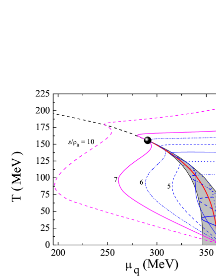
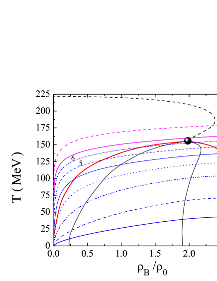
Figure 1: Left panel: QCD phase diagram in the $T-\mu_{q}$ plane. The full red line is the first-order chiral phase transition and the gray region is the unstable region bounded by the spinodal lines $-$ spinodal region. Right panel: QCD phase diagram in the $T-\rho_{B}/\rho_{0}$ plane with $\rho_{0}=0.16$ fm^-3. The full red line delineates the phase coexistence boundary (binodal line). The metastable region is bounded externally by the the binodal line and is separated from the unstable region by the spinodal lines (gray lines). For both panels the isentropic trajectories correspond to (from right) $S/\rho_{B}=$ [0.5, 1, 2, 3, 4, 5, 6, 7, 10]. The isentropic trajectories in magenta intersect the crossover line.

In this section, we consider three different scenarios for the phase diagram:
Case I $-$ equal quark chemical potentials ($\mu_{u}=\mu_{d}=\mu_{s}$). This scenario, used in most calculations, corresponds to zero charge (or isospin), $\mu_{Q}=0$, and zero strangeness chemical potential, $\mu_{S}=0$. It also allows for isospin symmetry, $M_{u}=M_{d}$, and the net strange quark density, $\rho_{s}$, is nonzero.

Case II$-$ equal $u$ and $d$ quark chemical potentials ($\mu_{u}=\mu_{d}$) and zero strange quark chemical potential ($\mu_{s}=0$). It corresponds to zero charge (isospin) chemical potential, $\mu_{Q}=0$, and the strangeness chemical potential is one third of the total baryonic chemical potential, $\mu_{S}=1/3\mu_{B}$. This is the relevant scenario to simulate matter created by ultra relativistic HIC. Indeed, since thermalization is reached within $10^{-22}$ sec (10-20 fm/c), the time scale of the strong interaction, the system is far from $\beta$-equilibrium. The net strange quark number should be zero before the beginning of hadronization in the expansion stage Greiner:1987tg so, the strange quark density must be set to zero, $\rho_{s}=0$.

Case III$-$ $\beta$-equilibrium matter corresponding to $\mu_{u}-\mu_{d}=\mu_{Q}=-\mu_{e}$ and $\mu_{d}=\mu_{s}$ ($\mu_{S}=0$).

Next, we present our results for isentropic trajectories close to the CEP. In Fig. 1 we plot the isentropic trajectories in the $T-\mu_{q}$ (left panel) and in the $T-\rho_{B}$ (right panel) planes for Case I. The CEP is located at ($T^{\,CEP}=$ 155 MeV, $\mu_{q}^{CEP}=$ 291 MeV) (see Table 1). At zero temperature, the phase diagram presents a first-order phase transition with $\mu_{q}^{crit}=361$ MeV being the critical chemical potential where the transition takes place Buballa:2003qv ; Costa:2010zw . At $\mu_{q}=0$, both chiral and deconfinement transitions are crossovers, being the respective pseudocritical temperatures at $T_{c}^{\chi}=222$ MeV and $T^{\Phi}_{c}=210$ MeV Costa:2010zw .

	$T$ [MeV]	$\mu_{q}$ [MeV]	$\rho_{B}/\rho_{0}$
Case I ($\mu_{u}=\mu_{d}=\mu_{s}$)	155	291	$1.98$
Case II ($\rho_{s}=0$)	157	296	$1.84$
Case III ($\beta$-equilibrium)	146	308	$1.71$

Table 1: Temperature, quark chemical potential and baryonic density for the CEP in the different scenarios considered ($\rho_{0}=0.16$ fm^-3).

By analyzing the behavior of the isentropic trajectories when $T\rightarrow 0$, we note that all isentropic trajectories terminate at the same point of the horizontal axes: $T=0$ and $\mu_{q}=367.7$ MeV, with $\mu_{q}=M_{q}^{vac}>\mu_{q}^{crit}$. This combination ($T=0,\,\,\mu_{q}=367.7$ MeV) corresponds to the vacuum. Indeed, for the chosen set of parameters, at $T=0$, the first-order transition point satisfies the condition $\mu_{q}^{crit}<M^{vac}_{q}$ Buballa:2003qv . This scenario implies the existence of a strong first-order phase transition from the vacuum solution $M_{q}=M^{vac}_{q}$ into the partially chiral restored phase with $M_{q}$ small when compared with $M^{vac}_{q}$. At the transition point, the density jumps from zero to a relatively large value.

According to the third law of thermodynamics, when $T\rightarrow 0$, also $s\rightarrow 0$, and therefore, for $s/\rho_{B}=const.$, we must require that $\rho_{B}\rightarrow 0$, which is fulfilled when $\mu_{q}=M_{q}^{vac}$ Costa:2010zw . In fact, at $\mu_{q}^{crit}$ and $T=0$, the total baryonic density jumps from zero to $\sim 2.5\rho_{0}$, equally carried by quarks $u$ and $d$ (the density of strange quarks, $\rho_{s}$, is still zero, and we only have $\rho_{s}\neq 0$ when $\mu_{q}>M_{s}$).

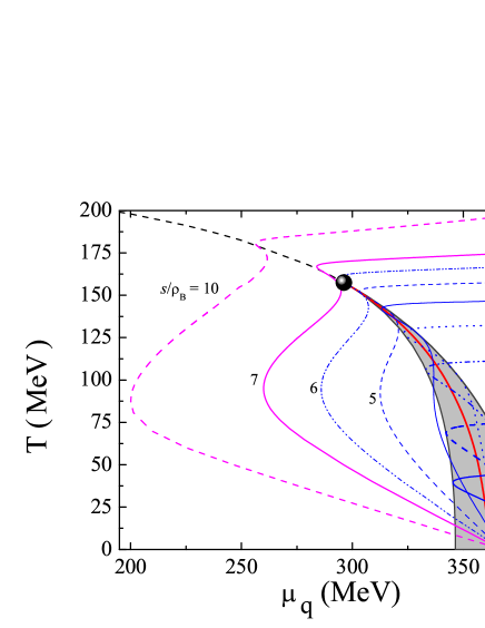
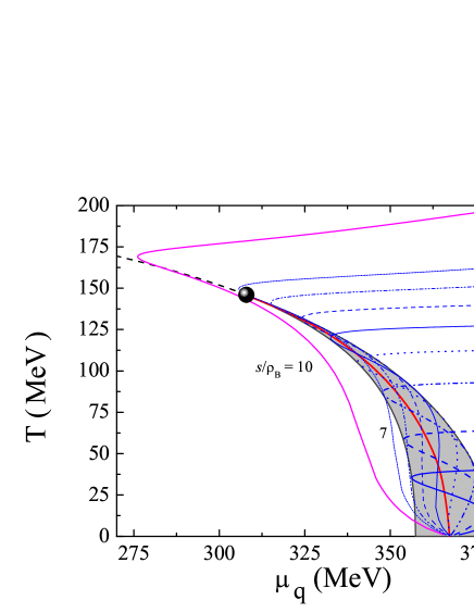
Figure 2: Left panel: Phase diagram in the $T-\mu_{q}$ plane for Case II ($\rho_{s}=0$). Right panel: Phase diagram in the $T-\mu_{q}$ plane for Case III ($\beta$-equilibrium). The isentropic trajectories in magenta intersect the crossover line.

In the vicinity of the first-order region, the isentropic trajectories with $s/\rho_{B}\lesssim 6$ come from the region of partially restored chiral symmetry and reach the unstable region (spinodal region), bounded by the spinodal lines, going then along with it as $T$ decreases until it reaches $T=0$ (see Fig. 1, left panel). Taking the line for $s/\rho_{B}=0.5$, it is seen that the isentropic trajectory intersects the spinodal line at ($T\approx 44$ MeV, $\mu_{q}\approx 372$ MeV) and crosses the first-order line twice, at ($T\approx 43$ MeV, $\mu_{q}\approx 358$ MeV) and ($T\approx 29$ MeV, $\mu_{q}\approx 360$ MeV), as the temperature decreases in a “zigzag”-shaped trajectory bounded by the spinodal lines. Now, taking the line with $s/\rho_{B}=4$, it becomes interesting to note that the isentropic trajectory starts by having a behavior similar that of $s/\rho_{B}=0.5$, but then it leaves the spinodal region. However, as the temperature decreases, the isentropic trajectory reaches the spinodal region again from lower values of $\mu_{q}$. This also happens for lines with $s/\rho_{B}=5$ and $s/\rho_{B}=6$.

For cases with $s/\rho_{B}>6$, the isentropic trajectories, given by the curves in magenta, go directly through the crossover region (the crossover is defined as the zero of the $\partial^{2}{\left\langle\bar{q}_{f}q_{f}\right\rangle}/\partial T^{2}$, i.e., the inflection point of the light quark condensates $\left\langle{\bar{q}_{f}q_{f}}\right\rangle$, $f=u,\,d$), displaying a smooth behavior, and they reach the spinodal region from lower values of $\mu_{q}$. In the crossover region, the isentropic trajectories have a behavior qualitatively similar to that obtained in lattice calculations Borsanyi:2012cr ; Ejiri:2005uv .

As already pointed out in Ref. Costa:2010zw , no focusing of isentropic trajectories towards the CEP is seen but only smooth trajectories. The focusing effect was suggested in Ref. Nonaka:2004pg , and it is argued that hot and dense QCD matter, as systems with a possible CEP of the same universality class as the three-dimensional Ising model, would exhibit focusing near the CEP: the CEP would act as an attractor for the isentropes Nonaka:2004pg . However, several models do not exhibit the focusing effect near the CEP. In Ref. Nakano:2009ps , isentropic trajectories were investigated in a renormalization group approach applied to the quark-meson model, and no focusing was found. Indeed, while the critical behavior at the CEP is universal, the focusing effect is not, because the the entropy per baryon does not diverge at the CEP. The characteristic shape of the isentropic trajectories in the vicinity of the CEP can vary from model to model, even if they belong to the same universality class Nakano:2009ps .

Next, we will proceed by investigating Case II (see left panel of Fig. 2) due to its relevance heavy-ion collisions. As already pointed out in Ref. Fukushima:2009dx , the phase diagram is only slightly changed by the constraint $\rho_{s}=0$; in our case the CEP moves from ($T^{\,CEP}=155$ MeV, $\mu_{q}^{CEP}=291$ MeV) to ($T^{\,CEP}=157$ MeV, $\mu_{q}^{CEP}=296$ MeV), as can be seen in Table 1. In Ref. Fukushima:2009dx it was also argued that the strangeness neutrality only has a perceptible effect on the isentropic trajectories at high temperatures. The reason for this behavior lies in the fact that the constituent mass of quark $s$, $M_{s}$, is still heavy around the chiral crossover when compared with the masses of the quarks $u$ and $d$, and consequently $\rho_{s}\approx 0$ even without a constraint, as long as $T$ is low and $\mu_{q}$ is smaller than $M_{s}$.

In right panel of Fig. 2, we present the results concerning Case III, matter in $\beta$-equilibrium, which has a large isospin asymmetry. The CEP for $\beta$-equilibrium occurs for a larger quark chemical potential, but also for a lower temperature when compared to the other scenarios. The reason is related to the fact that matter in $\beta$-equilibrium being less symmetric, is less bound, and therefore, the transition to a chirally symmetric phase occurs at a lower temperature and density than in the symmetric case Costa:2013zca . On the other hand, at $T=0$, the spinodal region is reduced by 10 MeV when compared with Cases I and II, where the spinodal region occurs between 346 and 378 MeV for both cases. Concerning the isentropic trajectories, the behavior is qualitatively similar to both cases previously studied, but they have some peculiarities, as can be seen in the right panel of Fig. 2: i) all isentropic trajectories will end at $T=0$ and $\mu_{q}=M_{q}^{vac}=\mu_{q}^{crit}=367.7$ MeV; and ii) for the same values of $s/\rho_{B}$, the isentropic trajectories occur at lower temperatures, especially for lower values of $s/\rho_{B}$.

III.2 Results at $G_{V}\neq 0$: The influence of the vector interaction on the isentropic trajectories

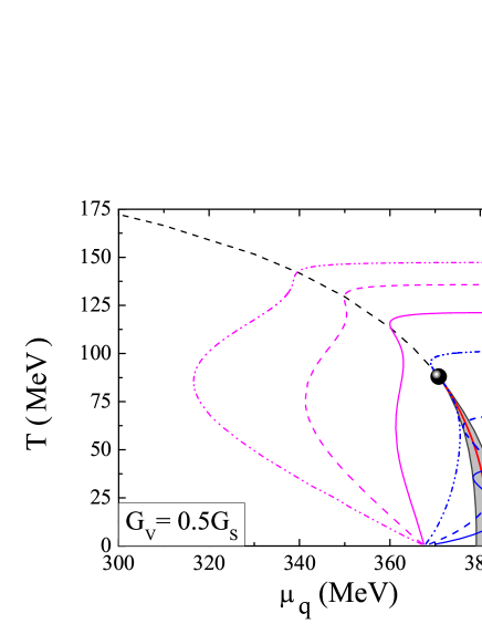
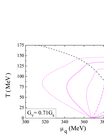
Figure 3: Phase diagram in the $T-\mu_{q}$ plane for $G_{V}=0.5G_{S}$ (left panel) and $G_{V}=G_{V}^{crit}=0.71G_{S}$ (right panel). For $G_{V}=G_{V}^{crit}=0.71G_{S}$ all the isentropic trajectories do not cross the first-order transition region.

In this section, we investigate the influence of the vector interaction in the isentropic trajectories. Henceforward, we restrict our study to Case I ($\mu_{u}=\mu_{d}=\mu_{s}$). The role of the vector interaction in the phase diagram was studied in detail in Ref. Fukushima:2008wg and more recently in Ref. Costa:2015bza , where the presence of an external magnetic field was also considered. It was shown that the CEP can be absent in the phase diagram when the value of the coupling $G_{V}$ is greater than the critical value of $G_{V}^{crit}\approx 0.71G_{S}$ within the present parametrization Costa:2015bza . Indeed, as the value of $G_{V}$ is increased from 0 to $G_{V}^{crit}$, the first-order phase transition is weakened: the CEP is located at lower temperatures and larger chemical potentials, but smaller densities. For $G_{V}=0.5G_{S}$, the CEP is located at ($T^{\,CEP}=88$ MeV, $\mu_{q}^{CEP}=371$ MeV), while at $G_{V}^{crit}\approx 0.71G_{S}$, it is located at ($T^{\,CEP}\sim 0$ MeV, $\mu_{q}^{CEP}=390$ MeV) (see Table 2).

	$T$ [MeV]	$\mu_{q}$ [MeV]	$\rho_{B}/\rho_{0}$
$G_{V}=0$ (Case I)	155	291	$1.98$
$G_{V}=0.5G_{S}$	88	371	$\sim 1.4$
$G_{V}^{crit}=0.71G_{S}$	$\sim 0$	390	$\sim 1.1$

Table 2: Temperature, quark chemical potential and baryonic density for the CEP for different values of the vector coupling, $G_{V}$ ($\rho_{0}=0.16$ fm^-3).

In the left (right) panel of Fig. 3, we present the results for the isentropic trajectories when $G_{V}=0.5G_{S}$ ($G_{V}^{crit}\approx 0.71G_{S}$). For $G_{V}=0.5G_{S}$ (left panel of Fig. 3), their behavior is different from that obtained with $G_{V}=0$ (left panel of Fig. 1): Due to the repulsive nature of the vector interaction, when $T=0$, the first-order phase transition only takes place at a critical potential $\mu_{q}^{crit}>M_{q}^{vac}$, meaning that the system will not form quark droplets; instead, the system has a homogeneous quark gas at low densities. The constituent mass of light quarks goes gradually down and the respective density starts to rise smoothly at $\mu_{q}\approx M_{q}^{vac}$, well before $\mu_{q}^{crit}$. Consequently, isentropic trajectories will not finish in the spinodal region as $T\rightarrow 0$ but for $\mu_{q}$ near $M_{q}^{vac}$. Taking the trajectory $s/\rho_{B}=1$ (dashed blue line), it intersects the first-order line three times, being the highest temperature crossing near the CEP. Then, as the temperature decreases in its path inside the spinodal region, it reaches the chemical potentials of both the lower and upper spinodal lines. At $T\approx 15$ MeV, the isentropic trajectory leaves the spinodal region to the chirally broken phase going to $\mu_{q}\sim M_{q}^{vac}$ when $T\rightarrow 0$. The trajectory with $s/\rho_{B}=2$ goes through the crossover at $T\approx 96$ MeV and $\mu_{q}\approx 369$ MeV, very close to the CEP ($T^{\,CEP}=88$ MeV, $\mu_{q}^{CEP}=371$ MeV), and comes into the spinodal region from lower values of $\mu_{q}$ just below the CEP. At $T\approx 70$ MeV, the isentropic trajectory leaves the spinodal region, its behavior being similar to that of the line $s/\rho_{B}=1$. The trajectories with $s/\rho_{B}\geq 3$ (in magenta) do not cross the spinodal region.

In the high-chemical-potential region, the isentropic trajectories behave similarly to Case I (see also the left panel of Fig. 1). In this region, the chiral symmetry is already restored for all scenarios, being the constituent masses of the quarks close to their current values. This also happens when $G_{V}^{crit}\approx 0.71G_{S}$ (see right panel of Fig. 3), even if in this case the first-order phase transition no longer occurs and the transition to the partially chiral restored phase is a crossover, except at the CEP where the transition is of second-order.

III.3 The influence of the magnetic field on the isentropic trajectories

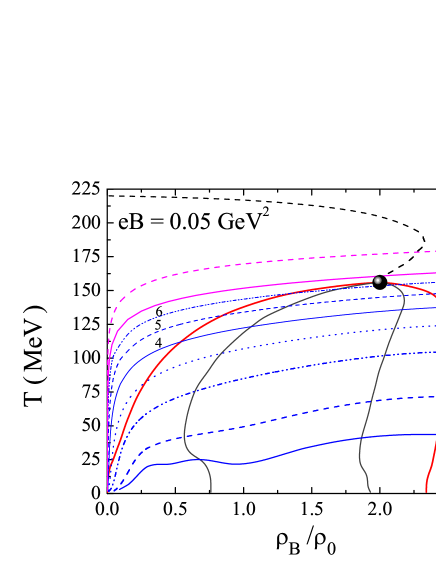
Figure 4: Left panel (right panel): Phase diagram in the $T-\mu_{q}$ ($T-\rho_{B}/\rho_{0}$) plane for $eB=0.05$ GeV². The isentropic trajectories correspond to (from right, counterclockwise) $S/\rho_{B}=$ [0.5, 1, 2, 3, 4, 5, 6, 7, 10 ]. The isentropic trajectories in magenta intersect the crossover line.

The influence of a magnetic field gives rise to a magnetic catalysis (MC) effect$-$i.e., the enhancement of the quark condensate due to the magnetic field. Increasing the chemical potential and/or the temperature and increasing the magnetic field have competing effects: while high chemical potentials and/or temperatures favor the restoration of chiral symmetry, the magnetic field has an opposite effect Avancini:2011zz .

The influence of external magnetic fields on the position of the CEP was investigated in detail for both NJL and PNJL models in Refs. Avancini:2012ee ; Costa:2013zca ; Costa:2015bza . The main conclusions when $\mu_{u}=\mu_{d}=\mu_{s}$ were that the trend is similar for both models: as the intensity of the magnetic field increases until a certain value ($eB\sim 0.4$ GeV² Costa:2013zca ; Costa:2015bza ), the transition temperature increases and the baryonic chemical potential decreases. For even stronger magnetic fields, when no inverse magnetic catalysis (IMC) effects are considered, both $T^{\,CEP}$ and $\mu_{B}^{CEP}$ increase Avancini:2012ee ; Costa:2013zca . This can be seen from Table 3. If the isospin symmetric matter scenario is taken, $\mu_{u}=\mu_{d}$ and $\mu_{s}=0$, the influence of the magnetic field on the CEP is very similar to the previous one, the temperature being only slightly larger and the baryonic density only slightly smaller for the CEP’s location Costa:2013zca .

When IMC effects Ferreira:2014kpa ; Ferreira:2013tba are taken into account, noticeable effects on the location of the CEP occur for sufficiently high values of the magnetic field: the CEP will now occur at increasingly smaller chemical potentials and at a practically unchanged temperature Costa:2015bza . Under an increase of the magnetic field, the CEP eventually moves toward $\mu_{B}=0$, and the deconfinement and chiral phase transitions should become of first-order as predicted by lattice calculations Endrodi:2015oba .

	$T$ [MeV]	$\mu_{q}$ [MeV]	$\rho_{B}/\rho_{0}$
$eB=0$ (Case I)	155	291	$1.98$
$eB=0.05$ GeV2	156	289	$\sim 2.0$
$eB=0.3$ GeV2	192	225	$\sim 3.5$

Table 3: Temperature, quark chemical potential and baryonic density for the CEP at $eB=0$, $eB=0.05$ GeV², and $eB=0.3$ GeV² ($\rho_{0}=0.16$ fm^-3).

To investigate the influence of the magnetic field on the behavior of isentropic trajectories we take $eB=0.05$ GeV², a relatively small magnetic field, and $eB=0.3$ GeV² (a magnetic field that could occur at LHC experiments, even if the magnetic field can only be produced for a short period of time in HIC), which are plotted in Figs. 4 and 5, respectively. No IMC effects on the location of CEP will be considered. From the panels of both figures, we conclude that as the magnetic field increases, the spinodal region is enlarged, especially for $eB=0.3$ GeV²: the extension of the spinodal region at $T=0$ goes from $\Delta\mu_{q}=32$ MeV for $eB=0$ to $\Delta\mu_{q}=167$ MeV for $eB=0.3$ GeV². A complete study of the effect of the magnetic field intensities on the EOS at $T=0$ was performed in Refs. Menezes:2014aka ; Costa:2015bza . As pointed out, for some ranges of the magnetic field, several first-order phase transitions occur which disappear when the temperature is slightly increased, so they will not influence the behavior of the chosen isentropic trajectories. In fact, like in our case for $eB=0.05$ GeV², the filling of the Landau levels originates Haas–van Alphen oscillations (the effect of Landau quantization of charged particles’ energy). Larger values of $B$ increase the amplitude of the fluctuations and reduce their number, because fewer Landau levels are involved Menezes:2014aka . The consequence is that the larger the intensity of the magnetic field, the greater the difficulty in restoring chiral symmetry. On the other hand, by increasing the temperature, thermal energy can become of the order of the level spacing and washes out these Landau quantization effects. Nevertheless, at sufficiently low temperatures, Landau quantization still manifests itself by the appearance of oscillations in physical quantities like the pressure.

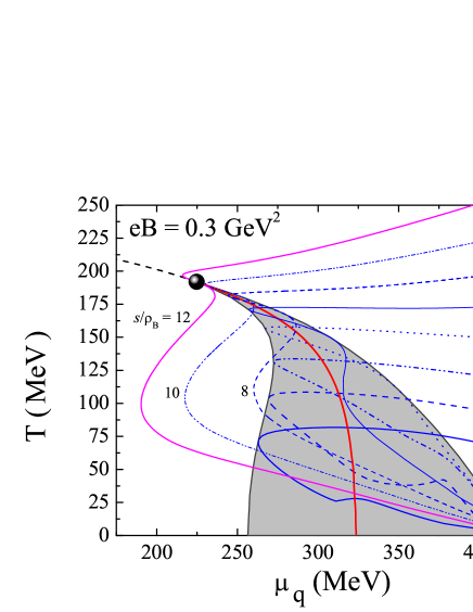
Figure 5: Left panel (right panel): Phase diagram in the $T-\mu_{q}$ ($T-\rho_{B}/\rho_{0}$) plane for $eB=0.3$ GeV². The isentropic trajectories correspond to (from right, counterclockwise) $S/\rho_{B}=$ [0.5, 1, 2, 4, 6, 8, 10, 12]. The isentropic trajectories in magenta intersect the crossover line.

The investigated isentropic trajectories are quite affected by the growth of the spinodal region as would be expected: there is an entrainment of the isentropes to higher temperatures within this region as it grows, due to the increasing of the magnetic field, as can be seen by comparing the left panels of Figs. 4 and 5. Together with the shift of the CEP (see Table 3) to higher (lower) temperatures (chemical potentials) by increasing magnetic fields (making the spinodal region bigger), also the isentropic trajectories are pushed to higher temperatures in the transition region, especially when $eB=0.3$ GeV².

However, outside of the spinodal region and for high chemical potentials, the isentropes have almost the same temperature as those with $eB=0$, in particular for $eB=0.05$ GeV². This can be understood by considering the fact that at high temperatures and chemical potentials, the restoration of chiral symmetry already took place and the magnetic catalysis effect is almost suppressed: due to the increasing temperature, more Landau Levels will be filled, when compared with low temperatures, being the system less affected by the magnetic field. For lower temperatures isentropes with $s/\rho_{B}<4$, at $eB=0.3$ GeV², are more affected by the magnetic field (as can be seen in left panel of Fig. 5), where they can decrease as $\mu_{q}$ is increased.

As in the previous sections, no focusing of isentropic trajectories towards the CEP is seen with increased magnetic field but only smooth trajectories, as with the results obtained in the model SU (2).

Finally, from the right panels of Figs. 4 and 5, it is seen that the baryonic density area of the transition region increases as the magnetic field increases. This is the result of the strengthening of the first-order transition due to the magnetic field. As already mentioned, stronger magnetic fields induce larger spacing between the Landau levels, and consequently, it is more difficult to restore chiral symmetry. On the other hand, for high magnetic fields, the lower-density spinodal line is pulled to very small densities, and some isentropes (see the case for $s/\rho_{B}=4$ in the right panel of Fig. 5) can reach the spinodal region for small values of the density. With this behavior, it is expected that the enhancement of fluctuations of observables caused by spinodal instabilities, like strangeness, will be more easily detected in the presence of strong magnetic fields.

IV Conclusions

In the present work we have investigated the isentropic trajectories around the CEP. The isentropic trajectories are very interesting because the hydrodynamical expansion of a HIC fireball nearly follows trajectories of constant entropy. New insights about the QCD phase diagram can be obtained by investigating these possible paths for the hydrodynamic evolution of a thermal medium created in the collisions. An unambiguous experimental identification of a first-order phase transition (if it exists) from the hadronic phase to the deconfined phase is one important goal of HIC experiments at present and future facilities. However, the first-order transition can be affected by the isospin or strangeness content of the medium, by the role of the vector interaction in the medium, or by external conditions, like the presence of an external magnetic field.

We considered different scenarios of interest for the phase diagram by choosing matter with different content of strangeness and isospin (the $\beta$-equilibrium case having the largest isospin asymmetry). We also explored the effects of the vector interaction and of an external magnetic field on the isentropic trajectories around the CEP.

More asymmetric matter weakens the first-order transition: the CEP for matter in $\beta$-equilibrium occurs at lower temperatures and densities than the symmetric cases ($\mu_{u}=\mu_{d}=\mu_{s}$ and $\mu_{u}=\mu_{d}$, $\mu_{s}=0$); at $T=0$ the spinodal region is also smaller for matter in $\beta$-equilibrium. Concerning the isentropic trajectories, the behavior is qualitatively similar for all cases investigated, but for the same values of $s/\rho_{B}$, the isentropic trajectories occur at lower temperatures for matter in $\beta$-equilibrium.

When a vector interaction is introduced, the first-order transition becomes even weaker, which is reflected in the CEP location (it can even disappear in the $\mu_{q}$ axis) and in an increasingly smaller area of instability as $G_{V}$ grows. In the high chemical potential region the isentropic trajectories behave similarly to the case without vector interaction once the chiral symmetry is already restored for all scenarios and the influence of vector interaction fades out.

On the other hand, the influence of a strong magnetic field on the phase diagram is reflected in the strengthening of the first-order transition with the respective enlargement of the spinodal region and the displacement of the CEP to higher temperatures and lower chemical potentials. The isentropic trajectories are entrained for higher temperatures, and the ones with lower values of $s/\rho_{B}$ at lower temperatures are more affected by the magnetic field, especially for higher values of $B$. For high magnetic fields, the lower-density spinodal line is pulled to small densities, and some isentropes can reach the spinodal region for small values of the density. It is then expected that there will be an enhancement of fluctuations of observables caused by spinodal instabilities in the presence of strong magnetic fields at lower densities.

Acknowledgment:

I would like to thank C. Providência and J. Moreira for helpful discussions. This work was supported by “Fundação para a Ciência e Tecnologia”, Portugal, under Grant No. SFRH/BPD/102273/2014.

Appendix A

The flavor contributions from vacuum $\Omega_{\text{vac}}^{f}$, medium $\Omega_{\text{med}}^{f}$, and magnetic field $\Omega_{\text{mag}}^{f}$ Menezes:2008qt ; Menezes:2009uc are given by

$$\Omega_{\text{vac}}^{f} =-6\int_{\Lambda}\frac{d^{3}p_{f}}{(2\pi)^{3}}E_{f},$$ (6)

$$\Omega_{\text{med}}^{f} =-T\frac{|q_{f}B|}{2\pi}\sum_{n=0}\alpha_{n}\int_{-\infty}^{+\infty}\frac{dp_{z}^{i}}{2\pi}\left(Z_{\Phi}^{+}(E_{f})+Z_{\Phi}^{-}(E_{f})\right),$$ (7)

$$\Omega_{\text{mag}}^{f} =-\frac{3(|q_{f}|B)^{2}}{2\pi^{2}}\left[\zeta^{{}^{\prime}}(-1,x_{f})-\frac{1}{2}(x_{f}^{2}-x_{f})\ln x_{f}+\frac{x_{f}^{2}}{4}\right],$$ (8)

where $E_{f}=\sqrt{(p_{z}^{i})^{2}+M_{f}^{2}+2|q_{f}|Bk}$ , $\alpha_{0}=1$ and $\alpha_{k>0}=2$, $x_{f}=M_{f}^{2}/(2|q_{f}|B)$, and $\zeta^{{}^{\prime}}(-1,x_{f})=d\zeta(z,x_{f})/dz|_{z=-1}$, where $\zeta(z,x_{f})$ is the Riemann-Hurwitz zeta function. $Z_{\Phi}^{+}$ and $Z_{\Phi}^{-}$ read

$$Z_{\Phi}^{+}=\ln\Big{\{}1+3\bar{\Phi}e^{-\beta(E_{f}-\mu_{f})} +3\Phi e^{-2\beta(E_{f}-\mu_{f})}$$

$$+e^{-3\beta(E_{f}-\mu_{f})}\Big{\}},$$ (9)

$$Z_{\Phi}^{-}=\ln\Big{\{}1+3\Phi e^{-\beta(E_{f}+\mu_{f})} +3\bar{\Phi}e^{-2\beta(E_{f}+\mu_{f})}$$

$$+e^{-3\beta(E_{f}+\mu_{f})}\Big{\}}.$$ (10)

The quark condensates $\left\langle\bar{\psi}_{f}\psi_{f}\right\rangle$ are given by $\left\langle\bar{\psi}_{f}\psi_{f}\right\rangle=\left\langle\bar{\psi}_{f}\psi_{f}\right\rangle_{\text{vac}}+\left\langle\bar{\psi}_{f}\psi_{f}\right\rangle_{\text{mag}}+\left\langle\bar{\psi}_{f}\psi_{f}\right\rangle_{\text{med}},$ where

$$\left\langle\bar{\psi}_{f}\psi_{f}\right\rangle_{\text{vac}} =-6\int_{\Lambda}\frac{d^{3}p}{(2\pi)^{3}}\frac{M_{f}}{E_{f}},$$ (11)

$$\left\langle\bar{\psi}_{f}\psi_{f}\right\rangle_{mag}=-\frac{3m_{f}|q_{f}|B}{2\pi^{2}} \Big{[}\ln\Gamma(x_{i})-\frac{1}{2}\ln(2\pi)+x_{i}$$

$$-\frac{1}{2}(2x_{f}-1)\ln(x_{f})\Big{]},$$ (12)

$$\left\langle\bar{\psi}_{f}\psi_{f}\right\rangle_{\text{med}} =\frac{3(|q_{f}|B)^{2}}{2\pi}$$

$$\times\sum_{n}\alpha_{n}\int_{-\infty}^{+\infty}\frac{dp_{z}^{i}}{2\pi}\left(f_{\Phi}^{+}(E_{f})+f_{\Phi}^{-}(E_{f})\right).$$ (13)

The distribution functions $f_{\Phi}^{+}$ and $f_{\Phi}^{-}$ are

$$f_{\Phi}^{+}(E_{f}) =\frac{\bar{\Phi}e^{-\beta(E_{f}-\mu_{f})}+2\Phi e^{-2\beta(E_{f}-\mu_{f})}+e^{-3\beta(E_{f}-\mu_{f})}}{1+3\bar{\Phi}e^{-\beta(E_{f}-\mu_{f})}+3\Phi e^{-2\beta(E_{f}-\mu_{f})}+e^{-3\beta(E_{f}-\mu_{f})}},$$

$$f_{\Phi}^{-}(E_{f}) =\frac{\Phi e^{-\beta(E_{f}+\mu_{f})}+2\bar{\Phi}e^{-2\beta(E_{f}+\mu_{f})}+e^{-3\beta(E_{f}+\mu_{f})}}{1+3\Phi e^{-\beta(E_{f}+\mu_{f})}+3\bar{\Phi}e^{-2\beta(E_{f}+\mu_{f})}+e^{-3\beta(E_{f}+\mu_{f})}}.$$

By employing a mean-field approach the effective quark masses, $\Phi$, and $\bar{\Phi}$ can be obtained self-consistently from

$$M_{f}=m_{f}-4G_{S}\left\langle\bar{\psi}_{f}\psi_{f}\right\rangle-2G_{D}\epsilon_{ijk}\left\langle\bar{\psi}_{j}\psi_{j}\right\rangle\left\langle\bar{\psi}_{k}\psi_{k}\right\rangle$$

and

$$\frac{\partial{\cal U}}{\partial\Phi}=\frac{\partial{\cal U}}{\partial\bar{\Phi}}=0.$$ (17)

References

- (1) D. G. d’Enterria, J. Phys. G 34 (2007) S53, [nucl-ex/0611012].
- (2) R. Averbeck, J. W. Harris and B. Schenke, “Heavy-Ion Physics at the LHC,” The Large Hadron Collider: Harvest of Run 1, Springer (2015) 355-420.
- (3) M. Bluhm, B. Kampfer, R. Schulze, D. Seipt and U. Heinz, Phys. Rev. C 76 (2007) 034901, [arXiv:0705.0397 [hep-ph]].
- (4) C. DeTar, L. Levkova, S. Gottlieb, U. M. Heller, J. E. Hetrick, R. Sugar and D. Toussaint, Phys. Rev. D 81 (2010) 114504, [arXiv:1003.5682 [hep-lat]].
- (5) S. Borsanyi, G. Endrodi, Z. Fodor, S. D. Katz, S. Krieg, C. Ratti and K. K. Szabo, JHEP 1208 (2012) 053, [arXiv:1204.6710 [hep-lat]].
- (6) M. Asakawa, S. A. Bass, B. Muller and C. Nonaka, Phys. Rev. Lett. 101 (2008) 122302, [arXiv:0803.2449 [nucl-th]].
- (7) P. Senger, E. Bratkovskaya, A. Andronic, R. Averbeck, R. Bellwied, et al., Lect.Notes Phys. 814 (2011) 681–847.
- (8) G. Endrodi, Z. Fodor, S. D. Katz and K. K. Szabo, JHEP 1104, 001 (2011) [arXiv:1102.1356 [hep-lat]].
- (9) C. S. Fischer, J. Luecker and C. A. Welzbacher, Phys. Rev. D 90, no. 3, 034022 (2014) [arXiv:1405.4762 [hep-ph]].
- (10) P. Costa, M. C. Ruivo and C. A. de Sousa, Phys. Rev. D 77, 096001 (2008) [arXiv:0801.3417 [hep-ph]].
- (11) B. Hiller, J. Moreira, A. A. Osipov and A. H. Blin, Phys. Rev. D 81, 116005 (2010) [arXiv:0812.1532 [hep-ph]].
- (12) P. Costa, C. A. de Sousa, M. C. Ruivo and H. Hansen, Europhys. Lett. 86, 31001 (2009) [arXiv:0801.3616 [hep-ph]].
- (13) B. I. Abelev et al. [STAR Collaboration], Phys. Rev. C 81 (2010) 024911, [arXiv:0909.4131 [nucl-ex]].
- (14) L. Adamczyk et al. [STAR Collaboration], Phys. Rev. Lett. 113 (2014) 092301, [arXiv:1402.1558 [nucl-ex]].
- (15) T. Anticic et al. [NA49 Collaboration], Phys. Rev. C 81 (2010) 064907, [arXiv:0912.4198 [nucl-ex]].
- (16) M. Gazdzicki [NA49 and NA61/SHINE Collaborations], J. Phys. G 38 (2011) 124024, [arXiv:1107.2345 [nucl-ex]].
- (17) A. Aduszkiewicz et al. [NA61/SHINE Collaboration], arXiv:1510.00163 [hep-ex].
- (18) R. A. Lacey, Phys. Rev. Lett. 114 (2015) 142301, [arXiv:1411.7931 [nucl-ex]].
- (19) K. A. Bugaev, A. I. Ivanytskyi, D. R. Oliinychenko, V. V. Sagun, I. N. Mishustin, D. H. Rischke, L. M. Satarov and G. M. Zinovjev, arXiv:1412.0718 [nucl-th].
- (20) Y. Nara, A. Ohnishi and H. Stoecker, arXiv:1601.07692 [hep-ph].
- (21) Y. Aoki, G. Endrodi, Z. Fodor, S. D. Katz and K. K. Szabo, Nature 443, 675 (2006) [hep-lat/0611014].
- (22) Y. Aoki, S. Borsanyi, S. Durr, Z. Fodor, S. D. Katz, S. Krieg and K. K. Szabo, JHEP 0906 (2009) 088, [arXiv:0903.4155 [hep-lat]].
- (23) S. Borsanyi, Z. Fodor, C. Hoelbling, S. D. Katz, S. Krieg and K. K. Szabo, Phys. Lett. B 730 (2014) 99, [arXiv:1309.5258 [hep-lat]].
- (24) I. N. Mishustin, Eur. Phys. J. A 30 (2006) 311, [hep-ph/0609196].
- (25) B. Borderie et al. [INDRA Collaboration], Phys. Rev. Lett. 86 (2001) 3252, [nucl-ex/0103009].
- (26) Y. Akiba et al., arXiv:1502.02730 [nucl-ex].
- (27) P. Costa, M. Ferreira, H. Hansen, D. P. Menezes and C. Providência, Phys. Rev. D 89 (2014) 056013, [arXiv:1307.7894 [hep-ph]].
- (28) K. Fukushima, Phys. Rev. D 77 (2008) 114028, [arXiv:0803.3318 [hep-ph]].
- (29) P. Costa, M. Ferreira, D. P. Menezes, J. Moreira and C. Providência, Phys. Rev. D 92 (2015) 036012, [arXiv:1508.07870 [hep-ph]].
- (30) K. Fukushima, Phys. Lett. B 591 (2004) 277, [hep-ph/0310121].
- (31) C. Ratti, M. A. Thaler and W. Weise, Phys. Rev. D 73 (2006) 014019, [hep-ph/0506234].
- (32) S. P. Klevansky, Rev. Mod. Phys. 64 (1992) 649.
- (33) T. Hatsuda and T. Kunihiro, Phys. Rep. 247 (1994) 221, [hep-ph/9401310].
- (34) M. Buballa, Phys. Rept. 407 (2005) 205, [hep-ph/0402234].
- (35) S. Roessner, C. Ratti and W. Weise, Phys. Rev. D 75 (2007) 034007, [hep-ph/0609281].
- (36) O. Kaczmarek, F. Karsch, P. Petreczky and F. Zantow, Phys. Lett. B 543 (2002) 41, [hep-lat/0207002].
- (37) P. Rehberg, S. P. Klevansky, and J. Hufner, Phys. Rev. C 53 (1996) 410, [hep-ph/9506436].
- (38) K. Kamikado, T. Kunihiro, K. Morita and A. Ohnishi, PTEP 2013 (2013) 053D01, [arXiv:1210.8347 [hep-ph]].
- (39) K. Fukushima, Phys. Rev. D 79 (2009) 074015, [arXiv:0901.0783 [hep-ph]].
- (40) C. Greiner, P. Koch and H. Stoecker, Phys. Rev. Lett. 58 (1987) 1825.
- (41) P. Costa, M. C. Ruivo, C. A. de Sousa and H. Hansen, Symmetry 2 (2010) 1338, [arXiv:1007.1380 [hep-ph]].
- (42) S. Ejiri, F. Karsch, E. Laermann and C. Schmidt, Phys. Rev. D 73 (2006) 054506, [hep-lat/0512040].
- (43) C. Nonaka and M. Asakawa, Phys. Rev. C 71 (2005) 044904, [nucl-th/0410078].
- (44) E. Nakano, B.-J. Schaefer, B. Stokic, B. Friman and K. Redlich, Phys. Lett. B 682 (2010) 401, [arXiv:0907.1344 [hep-ph]].
- (45) S. S. Avancini, D. P. Menezes and C. Providencia, Phys. Rev. C 83 (2011) 065805.
- (46) S. S. Avancini, D. P. Menezes, M. B. Pinto and C. Providencia, Phys. Rev. D 85 (2012) 091901, [arXiv:1202.5641 [hep-ph]].
- (47) M. Ferreira, P. Costa, O. Lourenço, T. Frederico and C. Providência, Phys. Rev. D 89 (2014) 116011, [arXiv:1404.5577 [hep-ph]].
- (48) M. Ferreira, P. Costa, D. P. Menezes, C. Providência and N. Scoccola, Phys. Rev. D 89 (2014) 016002, [arXiv:1305.4751 [hep-ph]].
- (49) G. Endrodi, JHEP 1507 (2015) 173, [arXiv:1504.08280 [hep-lat]].
- (50) D. P. Menezes, M. B. Pinto, L. B. Castro, P. Costa and C. Providência, Phys. Rev. C 89 (2014) 055207, [arXiv:1403.2502 [nucl-th]].
- (51) D. P. Menezes, M. B. Pinto, S. S. Avancini, A. Perez Martinez, and C. Providência, Phys. Rev. C 79 (2009) 035807, [arXiv:0811.3361 [nucl-th]];
- (52) D. P. Menezes, M. B. Pinto, S. S. Avancini, and C. Providência, Phys. Rev. C 80 (2009) 065805, [arXiv:0907.2607 [nucl-th]].