Quantitative Test of the Evolution of Geant4 Electron Backscattering Simulation

Abstract

Evolutions of Geant4 code have affected the simulation of electron backscattering with respect to previously published results. Their effects are quantified by analyzing the compatibility of the simulated electron backscattering fraction with a large collection of experimental data for a wide set of physics configuration options available in Geant4. Special emphasis is placed on two electron scattering implementations first released in Geant4 version 10.2: the Goudsmit-Saunderson multiple scattering model and a single Coulomb scattering model based on Mott cross section calculation. The new Goudsmit-Saunderson multiple scattering model appears to perform equally or less accurately than the model implemented in previous Geant4 versions, depending on the electron energy. The new Coulomb scattering model was flawed from a physics point of view, but computationally fast in Geant4 version 10.2; the physics correction released in Geant4 version 10.2p01 severely degrades its computational performance. Problems observed in electron backscattering simulation in previous publications have been addressed by evolutions in the Geant4 geometry domain.

I Introduction

The simulation of electron backscattering based on Geant4 [1, 2] has been investigated in a variety of configurations [3, 4], as this observable is a sensitive probe of multiple and single scattering modeling in Monte Carlo codes for particle transport.

Apparent anomalies, leading to the suppression of backscattering, were observed in association with some physics configurations [3]; dedicated investigations [4] hinted that some of the step limitation algorithms related to the treatment of multiple scattering could be sensitive to peculiarities of the Geant4 geometry domain, while single scattering simulation appeared to be immune from such effects. The observed inconsistency of the backscattering simulation outcome, which appeared to depend on the configuration of the experimental setup in the simulation, precluded unequivocal quantification of the accuracy of Geant4 multiple and single scattering models and their relative comparison in [4]. These issues have been addressed in Geant4 10.1p02 and later versions, thus allowing consistent quantification of Geant4 capability to simulate electron backscattering in a variety of physics configurations and of their relative ability to reproduce experimental measurements.

Geant4 version 10.2 also includes two new electron scattering implementations and a new predefined PhysicsConstructor, which are quantitatively evaluated in an experimental test case for the first time in this paper. The Goudsmit-Saunderson [5, 6] multiple scattering model was completely reimplemented in Geant4 10.2 on the basis of a reworked analytical foundation of the code: although the new model retains the same class name present in previous Geant4 versions, the code is entirely new. A predefined PhysicsConstructor using the Goudsmit-Saunderson model was released for the first time in Geant4 10.2. A single scattering model based on the Mott cross section [7, 8, 9], which did not work properly in previous Geant4 versions, and for this reason could not be used in the tests of [3, 4], was modified to become functional in Geant4 10.2. This model extends the provision of methods to simulate electron scattering as a discrete process in Geant4, as an alternative to condensed history schemes usually adopted in particle transport through multiple scattering modeling.

This paper documents quantitatively the effects of these Geant4 evolutions on the fraction of backscattered electrons. This observable is the most basic probe of the simulation of electron scattering in particle transport codes; its assessment is preparative to the validation of more complex observables related to electron scattering, such as the energy and angular distributions of scattered particles. Special emphasis is given in the following section to the characterization of the new physics modeling options available in Geant4 with respect to experimental measurements, and the assessment of their capabilities in comparison to other, previously available, options. All the results are based on statistical data analysis methods to ensure their objectiveness.

TABLE I: Multiple and single scattering settings in the simulation configurations evaluated in this test

Configuration	Description	Process class	Model class	Version	Step Limitation	RangeFactor
Urban	Urban model, user step limit	G4eMultipleScattering	G4UrbanMscModel		Safety (default)	0.04 (default)
UrbanBRF	Urban model	G4eMultipleScattering	G4UrbanMscModel		DistanceToBoundary	0.01
WentzelBRF	WentzelVI model	G4eMultipleScattering	G4WentzelVIModel		DistanceToBoundary	0.01
WentzelBRFP	WentzelVI model, $\theta_{limit}$=0.15	G4eMultipleScattering	G4WentzelVIModel		DistanceToBoundary	0.01
GS	Goudsmit-Saunderson	G4eMultipleScattering	G4GoudsmitSaundersonModel	10.1	Safety	0.01
	Goudsmit-Saunderson, Molière	G4eMultipleScattering	G4GoudsmitSaundersonModel	10.2	SafetyPlus	0.12
GSBRF	Goudsmit-Saunderson	G4eMultipleScattering	G4GoudsmitSaundersonModel	10.1	DistanceToBoundary	0.01
	Goudsmit-Saunderson, Molière	G4eMultipleScattering	G4GoudsmitSaundersonModel	10.2	DistanceToBoundary	0.12
GSBRF1	Goudsmit-Saunderson	G4eMultipleScattering	G4GoudsmitSaundersonModel	10.2	DistanceToBoundary	0.01
GSERF	Goudsmit-Saunderson, Molière	G4eMultipleScattering	G4GoudsmitSaundersonModel	10.2	Safety	0.12
GSPWA	Goudsmit-Saunderson, PWA	G4eMultipleScattering	G4GoudsmitSaundersonModel	10.2	SafetyPlus	0.12
GSPWABRF	Goudsmit-Saunderson, PWA	G4eMultipleScattering	G4GoudsmitSaundersonModel	10.2	DistanceToBoundary	0.12
GSPWAERF	Goudsmit-Saunderson, PWA	G4eMultipleScattering	G4GoudsmitSaundersonModel	10.2	Safety	0.12
Coulomb	Single scattering	G4CoulombScattering	G4eCoulombScatteringModel
CoulombMott	Single scattering, Mott	G4CoulombScattering	G4eSingleCoulombScatteringModel	10.2

TABLE II: Predefined Geant4 Electromagnetic PhysicsConstructors evaluated in this test

Configuration	PhysicsConstructor class	Version	Step Limitation	RangeFactor	ThetaLimit
EmLivermore	G4EmLivermorePhysics	10.1	DistanceToBoundary	0.01
		10.2	DistanceToBoundary	0.02
EmStd	G4EmStandardPhysics		Safety	0.04
EmOpt1	G4EmStandardPhysics_option1	10.1	Minimal	0.04
		10.2	Minimal	0.20
EmOpt2	G4EmStandardPhysics_option2	10.1	Minimal	0.04
		10.2	Minimal	0.20
EmOpt3	G4EmStandardPhysics_option3		DistanceToBoundary	0.04
EmOpt4	G4EmStandardPhysics_option4	10.1	SafetyPlus	0.02
		10.1p02, 10.1p03	DistanceToBoundary	0.02
		10.2	DistanceToBoundary	0.02
EmSS	G4EmStandardPhysicsSS		Safety	0.04	0
EmWVI	G4EmStandardPhysicsWVI	10.1	Safety	0.04	0.15
		10.2	Safety	0.04	0.02
EmGS	G4EmStandardPhysicsGS	10.2	SafetyPlus	0.12

II Simulation and Data Analysis Features

II-A Simulation configuration

The validation tests documented in this paper concern Geant4 versions from 10.1p02 to 10.2p02, which were released after the analyses reported in [3] and [4]. It is worthwhile to note that Geant4 version 10.1p03 is more recent than version 10.2. The documentation of the performance of a variety of Geant4 versions is relevant to the experimental community, where several versions of Geant4 are in use at the same time in different experiments, whose simulation production strategies do not always coincide with the rapid turnover of Geant4 version releases. It also provides significant information for the improvement of the Geant4 software development process and, more generally, for software engineering measurements relevant to large scale systems [10].

The experimental scenario and simulation execution environment pertinent to this paper are the same as in [3], where they are extensively described; interested readers can find detailed information in [3] and in the references cited therein. The additional details given below concern simulation features pertinent to Geant4 versions 10.1p02 to 10.2p02.

The physics configurations considered in this validation test are summarized in Tables I and II, which concern user-defined and predefined physics settings, respectively. Electron and photon interactions other than electron multiple and single scattering are based on the EEDL [11] and EPDL [12] data libraries [13, 14, 15] in the configurations listed in Table I, while in the configurations of Table II they are determined by the predefined physics settings pertinent to each PhysicsConstructor.

Predefined electromagnetic PhysicsConstructors in general use a combination of different electron scattering models and differ in the configuration of other electron and photon interactions; therefore it is difficult to ascertain the contribution of each physics modeling component to the accuracy of the simulated observable. Although some of them (G4EmStandardPhysicsGS, G4EmStandardPhysicsSS G4EmStandardPhysicsWVI) are defined as “experimental physics” in Geant4 user documentation associated with Geant4 version 10.2 [16], these PhysicsConstructors use theoretical models to describe electron and photon interactions with matter.

The user-defined physics configurations listed in Table I are intended to facilitate investigation of the effects of a multiple or single scattering model, with specified settings of options and parameters, on the simulated observable. For this purpose they instantiate a unique electron scattering process (multiple or single), with a unique model associated to it, and use the same configuration of electron-photon interactions other than electron scattering to highlight the effects specific to electron scattering modeling.

The new Goudsmit-Saunderson multiple scattering model first released in Geant4 10.2 can calculate the screening parameter according to the Molière formula (by default) or using elastic cross sections deriving from partial wave analysis calculations: the corresponding configurations are identified in Table I as “GS” and “GSPWA”, respectively. Additionally, it provides three step limitation algorithm options, identified as SafetyPlus, DistanceToBoundary and Safety. The SafetyPlus algorithm associated with the reimplemented Goudsmit-Saunderson model corresponds to the Safety step limitation algorithm associated with the Urban [17, 18] multiple scattering model, and is used by default; the DistanceToBoundary algorithm corresponds to the same option of the Urban model; the Safety algorithm corresponds to EGSnrc [19] error-free stepping algorithm. Therefore, six configurations related to the reimplemented Goudsmit-Saunderson model are considered in the validation analysis, which reflect the combination of options for the calculation of the screening parameter and for the step limitation algorithm; they are listed in Table I. Additionally, a configuration identified as “GSBRF1” is included in the test for the purpose of studying the effect of the RangeFactor parameter: it is identical to “GSBRF”, except for this different setting.

A predefined PhysicsConstructor G4EmStandardPhysicsGS, which uses the reimplemented Goudsmit-Saunderson multiple scattering model, was first introduced in Geant4 10.2 and is listed in Table II along with other previously released predefined PhysicsConstructors. In this class the Goudsmit-Saunderson model is configured with its default Molière screening and SafetyPlus step limitation options; additionally, the RangeFactor parameter is set to 0.12.

The new single scattering model released in Geant4 10.2 is associated with the G4eSingleCoulombScatteringModel class. The physics configuration which uses it is identified in this paper as “CoulombMott”. According to the Geant4 software documentation, this model is applicable to electrons of energy greater than 200 keV, incident on medium-light target nuclei [20].

Nevertheless, simulations involving this model were executed over all the experimental test cases considered in this paper, which span the range of atomic numbers from 4 to 92 and involve electron beam energies both below and above 200 keV, to characterize the behaviour of this model also outside its nominal applicability. This extended investigation is intended to quantify more objectively the capabilities of this model, considering that the qualitative definition of medium-light nuclei is susceptible to subjective interpretation and that electrons that are originally incident on the target with energy greater than the documented 200 keV threshold of applicability lose energy in the course of the transport due to interactions with the traversed medium. The results of using G4eSingleCoulombScatteringModel outside its nominal range of applicability are discussed in section III-D. It is worthwhile to note that no warnings of improper use of this model were issued when it was invoked outside its nominal domain of applicability, nor were any exceptions thrown in the course of the execution of the simulations.

II-B Data Analysis

The validation test concerns the fraction of electrons that are backscattered from a semi-infinite or infinite target of pure elemental composition. The reference experimental data involved in the validation process are the same as in [3]; for all aspects related to experimental data the reader is invited to consult reference [3].

Compatibility between simulation and experiment, as well as differences in compatibility with experiment associated with different simulation configurations, are assessed by means of statistical methods that are described in detail in [3] and [4]. The Statistical Toolkit [21, 22] and R [23] are used as software instruments for data analysis.

For convenience, compatibility with experimental data is summarized by a variable defined as “efficiency”, which represents the fraction of test cases where the p-value resulting from goodness-of-fit tests is larger than the predefined significance level. The uncertainties on the efficiencies are calculated according to a method based on Bayes’ theorem [24], which delivers meaningful results also in limiting cases, i.e. for efficiencies very close to 0 or to 1, where the conventional method based on the binomial distribution [25] produces unreasonable values. Apart from these special cases, both methods deliver identical results within the number of significant digits reported in the following tables.

As discussed in [3], the results reported in section III are based on the Anderson-Darling [26, 27] goodness-of-fit test, since the outcome of other tests (Cramer-von Mises [28, 29], Kolmogorov-Smirnov [30, 31] and Watson [32]) is statistically equivalent.

Contingency tables are used for categorical data analysis, where simulation configurations represent categories. They are based on the results of the Anderson-Darling test; their entries count the number of test cases associated with a given simulation configuration for which the null hypothesis of compatibility between simulated and backscattered data is rejected or fails to be rejected. It is worth stressing that what is compared in contingency tables is the capability of the simulation configurations subject to test to produce a fraction of backscattered electrons statistically compatible with experiment, not the backscattering fraction simulated with different configurations.

A variety of tests is applied to mitigate the risk of systematic effects in categorical data analysis: Fisher’s exact test [33], Barnard’s exact test [34] using the Z-pooled statistic [35] and the CSM approximation, Boschloo’s exact test [36] and Pearson’s $\chi^{2}$ [37] test, when the entries in the cells of a table are consistent with its applicability. The power of tests for categorical data analysis is not well established yet; Boschloo’s test and Barnard’s exact test calculated using the Z-pooled statistic are deemed more powerful than Fisher’s exact test for the analysis of 2x2 contingency tables [38, 39, 40].

The significance level is set at 0.01 both for goodness-of-fit tests and for the analysis of contingency tables.

II-C Computational performance

The intrinsic characteristics of the simulations, which reproduce different experimental models in terms of target shape and size and are executed in a heterogeneous computational environment [3], allow only a qualitative appraisal of the computational performance associated with the various physics configurations considered in this paper. Nevertheless, this complementary information provides valuable guidance for practical use of the physics configurations examined in this paper in realistic experimental scenarios; it is therefore discussed in the following sections that document the results derived from the various simulation configurations.

The variability of the computational environment and of the experimental scenarios involved in the test is partly taken into account by rescaling the CPU (central processing unit) time spent for each simulation according to the hardware characteristics of the node where it was executed, and by evaluating the computational performance in relative terms, i.e. with respect to a configuration taken as a common reference for comparison (the “EmStd” configuration, unless otherwise specified).

A smaller number of events was generated in some simulations using G4eSingleCoulombScatteringModel than in the other simulation configurations due to the exceedingly slow computational performance associated with this model, which would have required an unsustainable amount of computing resources to produce a simulated data sample of the same size as in the other test cases. These smaller data samples are reflected in larger error bars appearing in some plots concerning G4eSingleCoulombScatteringModel.

TABLE III: Efficiency calculated for different simulation configurations and Geant4 versions, in three energy ranges

	1-20 keV				20-100 keV				$\geq$100 keV
Configuration	10.1p03	10.2	10.2p01	10.2p02	10.1p03	10.2	10.2p01	10.2p02	10.1p03	10.2	10.2p01	10.2p02
Urban	0.08$\pm$0.02	0.16$\pm$0.03	0.16$\pm$0.03	0.16$\pm$0.03	0.22$\pm$0.04	0.25$\pm$0.04	0.25$\pm$0.04	0.21$\pm$0.04	0.63$\pm$0.06	0.64$\pm$0.06	0.64$\pm$0.06	0.64$\pm$0.06
UrbanBRF	0.16$\pm$0.03	0.10$\pm$0.03	0.16$\pm$0.03	0.16$\pm$0.03	0.33$\pm$0.04	0.29$\pm$0.04	0.38$\pm$0.04	0.39$\pm$0.04	0.68$\pm$0.06	0.63$\pm$0.06	0.63$\pm$0.06	0.63$\pm$0.06
GS	0.51$\pm$0.04	0.57$\pm$0.04	0.56$\pm$0.04	0.56$\pm$0.04	0.32$\pm$0.04	0.18$\pm$0.04	0.16$\pm$0.04	0.16$\pm$0.04	0.77$\pm$0.06	0.52$\pm$0.07	0.55$\pm$0.06	0.55$\pm$0.06
GSBRF	0.37$\pm$0.04	0.38$\pm$0.04	0.57$\pm$0.04	0.57$\pm$0.04	0.51$\pm$0.05	0.46$\pm$0.05	0.14$\pm$0.05	0.14$\pm$0.05	0.95$\pm$0.03	0.61$\pm$0.06	0.55$\pm$0.06	0.55$\pm$0.06
GSBRF1		0.35$\pm$0.04	0.42$\pm$0.04	0.42$\pm$0.04		0.45$\pm$0.05	0.44$\pm$0.05	0.45$\pm$0.05		0.61$\pm$0.06	0.59$\pm$0.06	0.57$\pm$0.06
GSERF		0.32$\pm$0.04	0.31$\pm$0.04	0.32$\pm$0.04		0.49$\pm$0.05	0.43$\pm$0.05	0.46$\pm$0.05		0.63$\pm$0.06	0.61$\pm$0.06	0.59$\pm$0.06
GSPWA		0.15$\pm$0.03	0.15$\pm$0.03	0.15$\pm$0.03		0.17$\pm$0.04	0.15$\pm$0.04	0.15$\pm$0.04		0.61$\pm$0.06	0.61$\pm$0.06	0.61$\pm$0.06
GSPWABRF		0.39$\pm$0.04	0.16$\pm$0.04	0.16$\pm$0.04		0.44$\pm$0.05	0.11$\pm$0.05	0.11$\pm$0.05		0.57$\pm$0.06	0.55$\pm$0.06	0.55$\pm$0.06
GSPWAERF		0.44$\pm$0.04	0.44$\pm$0.04	0.44$\pm$0.04		0.51$\pm$0.04	0.46$\pm$0.04	0.47$\pm$0.04		0.52$\pm$0.07	0.55$\pm$0.07	0.55$\pm$0.07
WentzelBRF	0.27$\pm$0.03	0.27$\pm$0.04	0.27$\pm$0.04	0.27$\pm$0.04	0.17$\pm$0.04	0.18$\pm$0.04	0.18$\pm$0.04	0.19$\pm$0.04	0.80$\pm$0.05	0.82$\pm$0.05	0.82$\pm$0.05	0.82$\pm$0.05
WentzelBRFP	0.47$\pm$0.04	0.35$\pm$0.04	0.35$\pm$0.04	0.35$\pm$0.04	0.45$\pm$0.04	0.44$\pm$0.04	0.43$\pm$0.04	0.43$\pm$0.04	0.86$\pm$0.05	0.86$\pm$0.05	0.84$\pm$0.05	0.84$\pm$0.05
Coulomb	0.49$\pm$0.04	0.36$\pm$0.04	0.36$\pm$0.04	0.37$\pm$0.04	0.46$\pm$0.05	0.46$\pm$0.05	0.46$\pm$0.05	0.46$\pm$0.05	0.80$\pm$0.05	0.79$\pm$0.05	0.79$\pm$0.05	0.80$\pm$0.05
CoulombMott		$<$0.01	$<$0.01	$<$0.01		$<$0.01	0.16$\pm$0.03	0.16$\pm$0.03		$<$0.02	0.96$\pm$0.03	0.96$\pm$0.03
EmLivermore	0.13$\pm$0.03	0.11$\pm$0.03	0.11$\pm$0.03	0.11$\pm$0.03	0.29$\pm$0.04	0.24$\pm$0.04	0.24$\pm$0.04	0.25$\pm$0.04	0.61$\pm$0.06	0.61$\pm$0.06	0.61$\pm$0.06	0.61$\pm$0.06
EmStd	0.13$\pm$0.03	0.08$\pm$0.03	0.08$\pm$0.03	0.08$\pm$0.03	0.19$\pm$0.04	0.16$\pm$0.03	0.16$\pm$0.03	0.16$\pm$0.03	0.71$\pm$0.06	0.86$\pm$0.05	0.86$\pm$0.05	0.86$\pm$0.05
EmOpt1	$<$0.01	$<$0.01	$<$0.01	$<$0.01	$<$0.01	$<$0.01	$<$0.01	$<$0.01	0.41$\pm$0.06	0.39$\pm$0.06	0.39$\pm$0.06	0.39$\pm$0.06
EmOpt2	$<$0.01	$<$0.01	$<$0.01	$<$0.01	$<$0.01	$<$0.01	$<$0.01	$<$0.01	0.41$\pm$0.06	0.39$\pm$0.06	0.39$\pm$0.06	0.39$\pm$0.06
EmOpt3	0.21$\pm$0.03	0.17$\pm$0.03	0.17$\pm$0.03	0.17$\pm$0.03	0.14$\pm$0.03	0.19$\pm$0.04	0.19$\pm$0.04	0.19$\pm$0.04	0.68$\pm$0.06	0.75$\pm$0.06	0.75$\pm$0.06	0.75$\pm$0.06
EmOpt4	0.23$\pm$0.03	0.10$\pm$0.03	0.10$\pm$0.03	0.10$\pm$0.03	0.21$\pm$0.04	0.24$\pm$0.04	0.24$\pm$0.04	0.24$\pm$0.04	0.73$\pm$0.06	0.66$\pm$0.06	0.66$\pm$0.06	0.68$\pm$0.06
EmWVI	0.45$\pm$0.04	0.36$\pm$0.04	0.36$\pm$0.04	0.36$\pm$0.04	0.46$\pm$0.05	0.47$\pm$0.05	0.47$\pm$0.05	0.47$\pm$0.05	0.82$\pm$0.05	0.82$\pm$0.05	0.82$\pm$0.05	0.82$\pm$0.05
EmSS	0.46$\pm$0.04	0.35$\pm$0.04	0.35$\pm$0.04	0.35$\pm$0.04	0.51$\pm$0.05	0.53$\pm$0.05	0.53$\pm$0.05	0.53$\pm$0.05	0.82$\pm$0.05	0.82$\pm$0.05	0.82$\pm$0.05	0.82$\pm$0.05
EmGS		0.58$\pm$0.04	0.58$\pm$0.04	0.58$\pm$0.04		0.18$\pm$0.04	0.19$\pm$0.04	0.19$\pm$0.04		0.54$\pm$0.06	0.50$\pm$0.06	0.50$\pm$0.06

III Results

TABLE IV: P-values deriving from the analysis of contingency tables that compare the compatibility with experiment obtained with different configuration options of the Goudsmit-Saunderson model in Geant4 10.2p02

	GSBRF $<$20 keV					GSPWAERF 20-100 keV					GSPWA $\geq$100 keV
Configuration	Fisher	$\chi^{2}$	Z-pooled	Boschloo	CSM	Fisher	$\chi^{2}$	Z-pooled	Boschloo	CSM	Fisher	$\chi^{2}$	Z-pooled	Boschloo	CSM
GS	0.903	0.807	0.873	0.850	0.763	$<0.001$	$<0.001$	$<0.001$	$<0.001$	$<0.001$	0.702	0.566	0.681	0.615	0.498
GSBRF						$<0.001$	$<0.001$	$<0.001$	$<0.001$	$<0.001$	0.702	0.566	0.681	0.615	0.498
GSBRF1	0.015	0.011	0.013	0.012	0.022	0.789	0.688	0.753	0.731	0.750	1.000	0.847	0.917	1.000	0.737
GSERF	$<0.001$	$<0.001$	$<0.001$	$<0.001$	$<0.001$	0.893	0.789	0.853	0.836	0.984	1.000	0.847	0.917	1.000	0.737
GSPWA	$<0.001$	$<0.001$	$<0.001$	$<0.001$	$<0.001$	$<0.001$	$<0.001$	$<0.001$	$<0.001$	$<0.001$
GSPWABRF	$<0.001$	$<0.001$	$<0.001$	$<0.001$	$<0.001$	$<0.001$	$<0.001$	$<0.001$	$<0.001$	$<0.001$	0.702	0.566	0.681	0.615	0.498
GSPWAERF	0.039	0.029	0.033	0.033	0.058						0.702	0.566	0.681	0.615	0.498
EmGS	1.000	0.902	0.949	1.000	0.861	$<0.001$	$<0.001$	$<0.001$	$<0.001$	$<0.001$	0.342	0.254	0.280	0.280	0.277

TABLE V: Efficiency of Goudsmit-Saunderson configurations with RangeFactor-0.10 in a simulation environment based on Geant4 10.2p01

Option	$<$20 keV	20-100 keV	$\geq$100 keV
GS	0.65 $\pm$ 0.04	0.21 $\pm$ 0.04	0.54 $\pm$ 0.06
GSBRF	0.62 $\pm$ 0.04	0.20 $\pm$ 0.04	0.54 $\pm$ 0.06
GSERF	0.37 $\pm$ 0.04	0.47 $\pm$ 0.04	0.57 $\pm$ 0.06
GSPWA	0.19 $\pm$ 0.03	0.21 $\pm$ 0.04	0.64 $\pm$ 0.06
GSPWABRF	0.18 $\pm$ 0.04	0.15 $\pm$ 0.03	0.63 $\pm$ 0.06
GSPWAERF	0.43 $\pm$ 0.04	0.47 $\pm$ 0.05	0.59 $\pm$ 0.06

III-A General overview

The efficiencies resulting from the Anderson-Darling goodness-of-fit test are reported in Table III for all the simulation configurations considered in this validation test; they are listed for Geant4 versions 10.1p03, 10.2, 10.2p01 and 10.2p02. The efficiencies for Geant4 10.1p02 are the same as for 10.1p03 within the number of significant digits appearing in Table III; those for 10.2p01 and 10.2p02 appear very similar. The outcome of the validation tests is discussed in detail in the following sections, with emphasis on the new physics models first introduced in Geant4 version 10.2 and the evolution with respect to previously published results.

Experimental uncertainties are reported in the plots discussed in the following sections when they are documented in the corresponding publications; statistical uncertainties of the simulated data that are smaller than the marker size are not visible in the figures.

III-B Dependencies Between Physics and Geometry Domains

Corrections to the Geant4 geometry domain were included in Geant4 10.1p02 to address the issues of apparent interplay with some multiple scattering simulation features described in [4]. These corrections fix the problem in Geant4 10.1p02 when the target and the detection hemisphere are adjacent (i.e. they share the boundary surface), but anomalies are still noticeable in simulations based on that version when the two geometrical components of the experimental model are displaced. This issue was addressed by further corrections implemented in Geant4 10.2 and later released also in Geant4 10.1p03. These two sets of corrections solve the problems described in [4].

The results reported in this paper were produced with adjacent target and detector hemisphere; they are exempt from the previously mentioned problems related to the geometrical configuration.

III-C Goudsmit-Saunderson Multiple Scattering Model

The data analysis concerning the Goudsmit-Saunderson multiple scattering addresses a few distinct issues: evaluating whether the options for the screening parameter and step limitation significantly affect the compatibility with backscattering measurements, determining whether the new implementation of the Goudsmit-Saunderson model in Geant4 10.2 and following patches significantly improves the validation results over the model implemented in Geant4 10.1p03, and objectively quantifying the capability of simulations using the Goudsmit-Saunderson model to reproduce experimental data with respect to other physics configurations. Contingency tables, based on the results of the Anderson-Darling test, specific to each topic of investigation are built for this purpose over the three energy ranges considered in this paper and analyzed by means of the tests documented in Section II-B.

The results of the tests are reported below for Geant4 10.2p02; the same conclusions also hold for the implementation in Geant4 10.2p01.

In each energy range, the configuration option of the Goudsmit-Saunderson model implemented in Geant4 10.2p02 that produces the highest efficiency is taken as a reference for comparison with other options and with the results produced with the previous implementation in Geant4 10.1p03: the GSPWA configuration option above 100 keV, the GSPWAERF option in the 20-100 keV range and the GSBRF option below 20 keV.

III-C1 Evaluation of modeling options

The backscattering fraction simulated with the different options of the Goudsmit-Saunderson model available in Geant4 10.2p02 is illustrated in Fig. 1 for a sample of target elements, along with experimental measurements. The plots also report the simulation results obtained with the GSBRF configuration in Geant4 10.1p03.

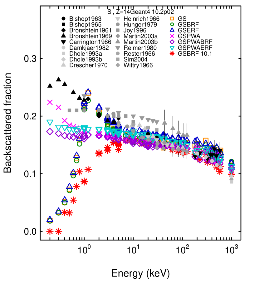
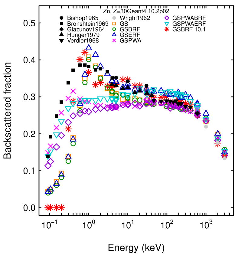
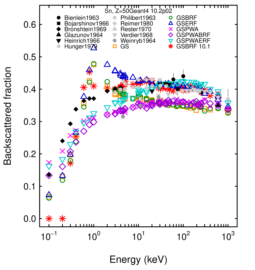
Figure 1: Measured and simulated fraction of backscattered electrons produced with the Goudsmit-Saunderson multiple scattering model: experimental data (black and grey filled markers); simulation with Geant4 10.2p02 GS (orange empty squares), GSBRF (green empty circles), GSERF (blue empty upward triangles), GSPWA (magenta crosses), GSPWABRF (violet empty diamonds), GSPWAERF (turquoise empty downward triangles) configurations, and simulation with Geant4 10.1p03 GSBRF configuration (red asterisks). The plots concern silicon, zinc, tin and gold targets.

All the Goudsmit-Saunderson configurations corresponding to different screening parameter and step limitation options available in Geant4 10.2p02 appear to achieve similar efficiency above 100 keV, while some differences are visible at lower energies in Table III. These qualitative observations are quantified through categorical data tests. The results of testing the hypothesis of equivalent compatibility with experiment with respect to the three reference options are documented in Table IV.

All tests fail to reject the null hypothesis above 100 keV, while at lower energies statistically significant differences in compatibility with experiment are identified with respect to the modeling options that produce the largest efficiency.

Only the GSPWAERF and GSBRF1 configuration options are not found inconsistent with the reference configurations over the whole energy range covered in the validation process. Some sensitivity to the value of the RangeFactor parameter is observed, as the hypothesis of equivalent compatibility with experiment with respect to the reference option is rejected for the GSBRF option between 20 and 100 keV, while it is not rejected for the GSBRF1 option. It is worthwhile to note that the null hypothesis is rejected in the test concerning the predefined G4EmStandardPhysicsGS PhysicsConstructor in the energy range between 20 and 100 keV, i.e. this simulation configuration does not represent an optimal choice of Goudsmit-Saunderson modeling options to reproduce experimental backscattering data at those energies.

The $\beta$-version of Geant4 recommends a lower value of the RangeFactor parameter (0.10 instead of 0.12) for the Goudsmit-Saunderson multiple scattering model in the predefined G4EmStandardPhysicsGs PhysicsConstructor; its effect on the compatibility of simulation with experiment obtained with the various model options has been investigated in the same simulation context as with Geant4 10.2p01 and is is documented in Table V. The efficiencies are qualitatively similar to those listed in Table III.

TABLE VI: P-values deriving from the analysis of contingency tables that compare the compatibility with experiment obtained with the Goudsmit-Saunderson model in Geant4 10.2p02 and 10.1p03

Geant4 10.2p02 GSBRF $<$20 keV

Geant4 10.2p02 GSPWAERF 20-100 keV

Geant4 10.2p02 GSPWA $>$100 keV

Geant4 10.1p03

Fisher

$\chi^{2}$

Z-pooled

Boschloo

CSM

Fisher

$\chi^{2}$

Z-pooled

Boschloo

CSM

Fisher

$\chi^{2}$

Z-pooled

Boschloo

CSM

GS

0.394

0.330

0.529

0.352

0.325

GSBRF

0.689

0.593

0.682

0.636

1.000

$<0.001$

$<0.001$

$<0.001$

$<0.001$

$<0.001$

TABLE VII: P-values of tests of contingency tables comparing the compatibility with experiment obtained by the GSBRF configuration with Geant4 10.1p03 and that obtained by other physics configurations with Geant4 10.2p02, above 100 keV

Configuration	Fisher	Z-pooled	Boschloo	CSM
Urban	$<0.001$	$<0.001$	$<0.001$	$<0.001$
UrbanBRF	$<0.001$	$<0.001$	$<0.001$	$<0.001$
WentzelBRF	0.074	0.047	0.048	0.094
WentzelBRFP	0.124	0.075	0.089	0.200
Coulomb	0.042	0.024	0.029	0.156
CoulombMott	1.000	0.751	1.000	1.000
EmLivermore	$<0.001$	$<0.001$	$<0.001$	$<0.001$
EmStd	0.203	0.126	0.156	0.471
EmOpt1	$<0.001$	$<0.001$	$<0.001$	$<0.001$
EmOpt2	$<0.001$	$<0.001$	$<0.001$	$<0.001$
EmOpt3	0.007	0.004	0.004	0.007
EmOpt4	$<0.001$	$<0.001$	$<0.001$	$<0.001$
EmWVI	0.074	0.047	0.048	0.094
EmSS	0.074	0.047	0.048	0.094
EmGS	$<0.001$	$<0.001$	$<0.001$	$<0.001$

TABLE VIII: P-values deriving from the analysis of contingency tables that compare the compatibility with experiment obtained with the Goudsmit-Saunderson model and with other simulation configurations in Geant4 10.2p02 below 100 keV

	Geant4 10.2p02 GSBRF $<$20 keV					Geant4 10.2p02 GSPWAERF 20-100 keV
Geant4 10.1p03	Fisher	$\chi^{2}$	Z-pooled	Boschloo	CSM	Fisher	$\chi^{2}$	Z-pooled	Boschloo	CSM
Urban	$<0.001$	$<0.001$	$<0.001$	$<0.001$	$<0.001$	0.001	0.001	0.001	0.001	0.001
UrbanBRF	$<0.001$	$<0.001$	$<0.001$	$<0.001$	$<0.001$	0.281	0.225	0.246	0.240	0.206
WentzelBRF	$<0.001$	$<0.001$	$<0.001$	$<0.001$	$<0.001$	$<0.001$	$<0.001$	$<0.001$	$<0.001$	$<0.001$
WentzelBRFP	$<0.001$	$<0.001$	$<0.001$	$<0.001$	$<0.001$	0.591	0.502	0.536	0.536	0.469
Coulomb	$<0.001$	$<0.001$	$<0.001$	$<0.001$	$<0.001$	0.893	0.789	0.853	0.836	0.984
CoulombMott	$<0.001$		$<0.001$	$<0.001$	$<0.001$	$<0.001$	$<0.001$	$<0.001$	$<0.001$	$<0.001$
EmLivermore	$<0.001$	$<0.001$	$<0.001$	$<0.001$	$<0.001$	0.001	0.001	0.001	0.001	0.001
EmStd	$<0.001$	$<0.001$	$<0.001$	$<0.001$	$<0.001$	$<0.001$	$<0.001$	$<0.001$	$<0.001$	$<0.001$
EmOpt1	$<0.001$		$<0.001$	$<0.001$	$<0.001$	$<0.001$		$<0.001$	$<0.001$	$<0.001$
EmOpt2	$<0.001$		$<0.001$	$<0.001$	$<0.001$	$<0.001$		$<0.001$	$<0.001$	$<0.001$
EmOpt3	$<0.001$	$<0.001$	$<0.001$	$<0.001$	$<0.001$	$<0.001$	$<0.001$	$<0.001$	$<0.001$	$<0.001$
EmOpt4	$<0.001$	$<0.001$	$<0.001$	$<0.001$	$<0.001$	$<0.001$	$<0.001$	$<0.001$	$<0.001$	$<0.001$
EmWVI	$<0.001$	$<0.001$	$<0.001$	$<0.001$	$<0.001$	1.000	1.000	1.000	1.000	1.000
EmSS	$<0.001$	$<0.001$	$<0.001$	$<0.001$	$<0.001$	0.504	0.423	0.532	0.462	1.000
EmGS	1.000	0.902	0.949	1.000	0.861	$<0.001$	$<0.001$	$<0.001$	$<0.001$	$<0.001$

TABLE IX: P-values deriving from contingency tables that compare the compatibility with experiment obtained with the most efficient predefined PhysicsConstructors in each energy range and using other simulation configurations, with Geant4 10.2p02

	EmGS $<$20 keV					EmSS 20-100 keV					EmStd $\geq$100 keV
Configuration	Fisher	$\chi^{2}$	Z-pooled	Boschloo	CSM	Fisher	$\chi^{2}$	Z-pooled	Boschloo	CSM	Fisher	$\chi^{2}$	Z-pooled	Boschloo	CSM
Urban	$<0.001$	$<0.001$	$<0.001$	$<0.001$	$<0.001$	$<0.001$	$<0.001$	$<0.001$	$<0.001$	$<0.001$	0.015	0.009	0.010	0.010	0.011
UrbanBRF	$<0.001$	$<0.001$	$<0.001$	$<0.001$	$<0.001$	0.060	0.044	0.048	0.048	0.047	0.009	0.005	0.006	0.006	0.006
GS	0.807	0.713	0.793	0.752	0.657	$<0.001$	$<0.001$	$<0.001$	$<0.001$	$<0.001$	0.001	$<0.001$	$<0.001$	$<0.001$	$<0.001$
GSBRF	1.000	0.902	0.949	1.000	0.861	$<0.001$	$<0.001$	$<0.001$	$<0.001$	$<0.001$	0.001	$<0.001$	$<0.001$	$<0.001$	$<0.001$
GSBRF1	0.011	0.008	0.009	0.009	0.016	0.285	0.229	0.250	0.250	0.571	0.003	0.002	0.002	0.002	0.002
GSEGSRF	$<0.001$	$<0.001$	$<0.001$	$<0.001$	$<0.001$	0.350	0.285	0.311	0.312	0.970	0.138	0.003	0.003	0.003	0.003
GSPWA	$<0.001$	$<0.001$	$<0.001$	$<0.001$	$<0.001$	$<0.001$	$<0.001$	$<0.001$	$<0.001$	$<0.001$	0.005	0.003	0.003	0.003	0.003
GSPWABRF	$<0.001$	$<0.001$	$<0.001$	$<0.001$	$<0.001$	$<0.001$	$<0.001$	$<0.001$	$<0.001$	$<0.001$	0.001	$<0.001$	$<0.001$	$<0.001$	$<0.001$
GSPWAEGSRF	0.029	0.021	0.024	0.024	0.041	0.504	0.423	0.532	0.462	1.000	0.001	$<0.001$	$<0.001$	$<0.001$	$<0.001$
WentzelBRF	$<0.001$	$<0.001$	$<0.001$	$<0.001$	$<0.001$	$<0.001$	$<0.001$	$<0.001$	$<0.001$	$<0.001$	0.798	0.607	0.681	0.653	1.000
WentzelBRFP	$<0.001$	$<0.001$	$<0.001$	$<0.001$	$<0.001$	0.181	0.141	0.154	0.154	0.244	1.000	0.792	0.870	1.000	1.000
Coulomb	$<0.001$	$<0.001$	$<0.001$	$<0.001$	$<0.001$	0.350	0.285	0.311	0.312	0.970	0.460	0.324	0.528	0.395	0.825
CoulombMott	$<0.001$		$<0.001$	$<0.001$	$<0.001$	$<0.001$	$<0.001$	$<0.001$	$<0.001$	$<0.001$	0.094		0.050	0.072	0.198
EmLivermore	$<0.001$	$<0.001$	$<0.001$	$<0.001$	$<0.001$	$<0.001$	$<0.001$	$<0.001$	$<0.001$	$<0.001$	0.005	0.003	0.003	0.003	0.003
EmStd	$<0.001$	$<0.001$	$<0.001$	$<0.001$	$<0.001$	$<0.001$	$<0.001$	$<0.001$	$<0.001$	$<0.001$
EmOpt1	$<0.001$		$<0.001$	$<0.001$	$<0.001$	$<0.001$		$<0.001$	$<0.001$	$<0.001$	$<0.001$	$<0.001$	$<0.001$	$<0.001$	$<0.001$
EmOpt2	$<0.001$		$<0.001$	$<0.001$	$<0.001$	$<0.001$		$<0.001$	$<0.001$	$<0.001$	$<0.001$	$<0.001$	$<0.001$	$<0.001$	$<0.001$
EmOpt3	$<0.001$	$<0.001$	$<0.001$	$<0.001$	$<0.001$	$<0.001$	$<0.001$	$<0.001$	$<0.001$	$<0.001$	0.234	0.154	0.209	0.176	0.274
EmOpt4	$<0.001$	$<0.001$	$<0.001$	$<0.001$	$<0.001$	$<0.001$	$<0.001$	$<0.001$	$<0.001$	$<0.001$	0.043	0.025	0.029	0.029	0.038
EmWVI	$<0.001$	$<0.001$	$<0.001$	$<0.001$	$<0.001$	0.504	0.423	0.532	0.462	1.000	0.798	0.607	0.681	0.653	1.000
EmSS	$<0.001$	$<0.001$	$<0.001$	$<0.001$	$<0.001$						0.798	0.607	0.681	0.653	1.000
EmGS						$<0.001$	$<0.001$	$<0.001$	$<0.001$	$<0.001$	$<0.001$	$<0.001$	$<0.001$	$<0.001$	$<0.001$

III-C2 Evaluation of the evolution of the implementation

The implementation of the Goudsmit-Saunderson multiple scattering model does not appear do have consistently evolved towards better compatibility with experiment from Geant4 10.1p03 to 10.2p02. Fig. 2 illustrates some examples of the evolution associated with the GSBRF simulation configuration.

A substantial drop in efficiency above 100 keV is observed in Table III with the Goudsmit-Saunderson multiple scattering implementation in Geant4 10.2 with respect to the value achieved with the implementation in Geant4 10.1p03, irrespective of the options selected for the calculation of the screening parameter and for the step limitation algorithm. The deterioration of compatibility with experiment is confirmed in the results obtained with the 10.2p01 and 10.2p02 versions. This decrease does not appear to be due to the larger value of the RangeFactor parameter recommended for the new implementation, as comparable results are obtained with the recommended value of 0.12 and with the value of 0.01 set in the GSBRF1 configuration, which is the same as in the simulation with the GSBRF configuration in the Geant4 10.1p03 environment. Since the efficiencies associated with simulation configurations involving other multiple scattering models (Urban and WentzelVI) remain statistically equivalent above 100 keV over the Geant4 versions considered in Table III, it is unlikely that the degradation of compatibility with experiment could originate from evolutions in Geant4 kernel code other than the implementation of Goudsmit-Saunderson multiple scattering.

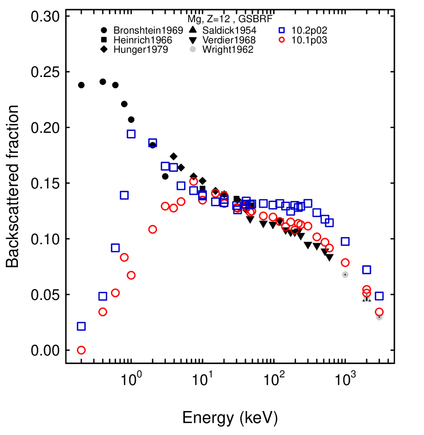
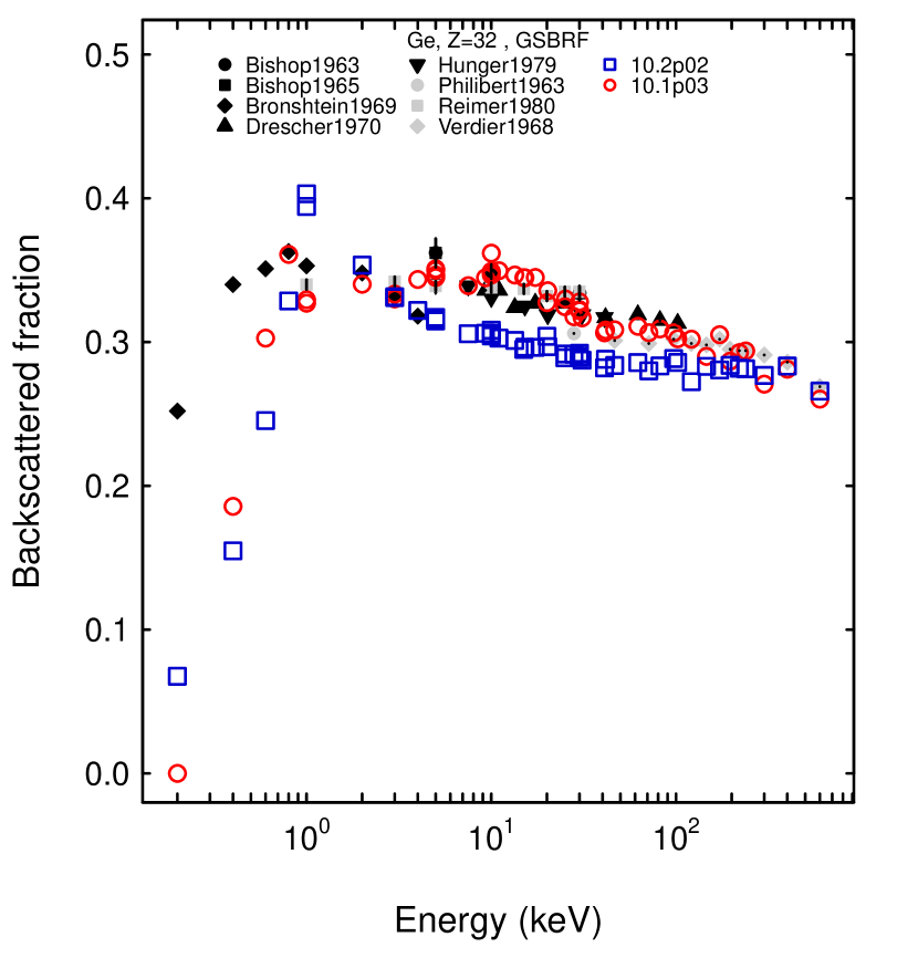
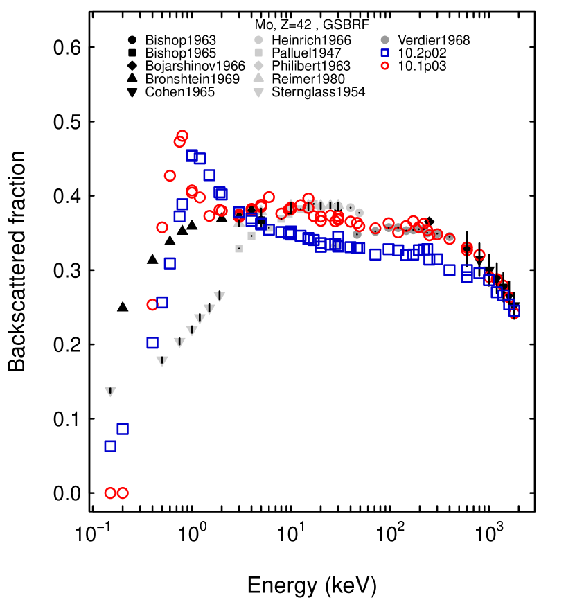
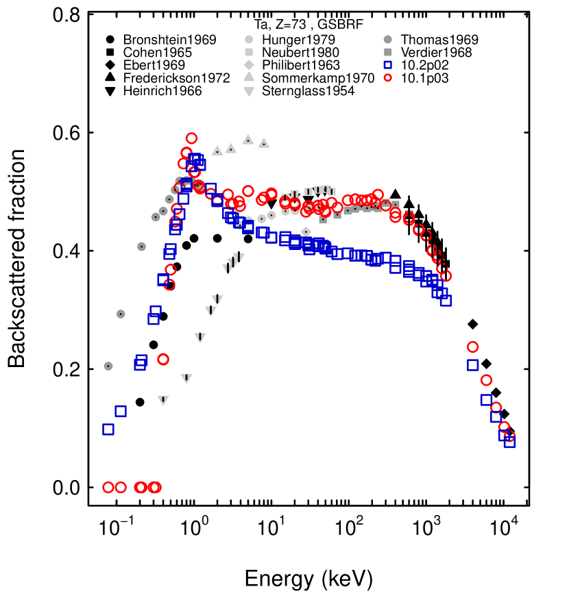
Figure 2: Measured and simulated fraction of backscattered electrons produced with the GSBRF configuration implementing the Goudsmit-Saunderson multiple scattering model: experimental data (black and grey filled markers); simulation with Geant4 10.2p02 (blue empty squares) and with Geant4 10.1p03 GSBRF configuration (red empty circles). The plots concern magnesium, germanium, molybdenum and tantalum targets.

The evolution of the capability to reproduce backscattering measurements is quantified through the test of contingency tables, which compare the compatibility with experiment achieved in each energy range by the Goudsmit-Saunderson configuration options associated with the highest efficiency in the Geant4 10.2p02 and 10.1p03 environment, respectively. Table VI reports the results of this test. The null hypothesis of equivalent compatibility with experiment is rejected above 100 keV, while it is not rejected at lower energies.

No substantial change regarding the comparison with the results deriving from Geant4 10.1.p03 is observed in the analysis of contingency tables produced with the lower RangeFactor value of 0.10.

From this analysis one can infer that the new implementation of the Goudsmit-Saunderson multiple scattering model, first released in Geant4 10.2, is equivalent to the previous one at reproducing experimental backscattering data below 100 keV, while it has negatively improved the compatibility of simulation with experiment above 100 keV.

Compatibility with experiment that is statistically equivalent to that obtained with the GSBRF configuration in the Geant4 10.1p03 environment can be achieved with configurations other than the Goudsmit-Saunderson options with Geant4 10.2p02 above 100 keV. The results of this analysis are summarized in Table VII, which reports the outcome of the tests of contingency tables involving the GSBRF configuration of Geant4 10.1p03 and other physics configurations pertinent to Geant4 10.2p02: the null hypothesis is not rejected for configurations including single scattering models and the WentzelVI model, either in user-defined or predefined PhysicsConstructors, and for the EmStd configuration.

III-C3 Evaluation with respect to other electron scattering models

This analysis is focused on the lower energy end, where simulation configurations encompassing the Goudsmit-Saunderson multiple scattering model are associated with relatively high efficiencies in the Geant4 10.2p02 environment.

Similarly to the previously documented evaluations, the GSBRF and GSPWAERF configurations, which achieve the largest efficiencies below 20 keV and in the 20-100 keV range, respectively, are considered as references in contingency tables, which compare their compatibility with experiment with that obtained with other simulation configurations in the context of Geant4 10.2p02. The results of these tests are summarized in Table VIII. Below 20 keV, the hypothesis of equivalent compatibility with experiment is rejected for all configurations with respect to the GSBRF configurations.

In the intermediate energy range the hypothesis of equivalent compatibility with experiment is not rejected for the UrbanBRF and WentzelBRF configurations, nor when using single scattering with the G4eCoulombScatteringModel instead of multiple scattering for electron transport. Consistent results are obtained regarding the EmSS and EmWVI predefined PhysicsConstructors, which use the WentzelVI and single Coulomb scattering models.

This analysis indicates that the Goudsmit-Saunderson implementation of Geant4 10.2p02 is significantly better than the other configurations subject to test at simulating electron backscattering below 20 keV, while it is statistically equivalent to other multiple and single scattering configurations available in the Geant4 10.2p02 environment in the 20-100 keV energy range. It should be noted, however, that the efficiencies at lower energies are substantially lower than those achieved above 100 keV by the most efficient configurations.

The lower RangeFactor value foreseen for Geant4 10.3-beta, mentioned in the previous subsection III-C2, does not substantially change the outcome of the comparisons with other electron scattering models.

III-D Single Scattering Model Based on the Mott Cross Section

No backscattered electrons are observed in simulations using the single scattering model based on the Mott cross section included in Geant4 10.2. The cause of this anomaly was corrected in the version released in Geant4 10.2p01.

The efficiency of simulations involving the CoulombMott configuration is documented in Table III: it is low below 100 keV, consistent with the documented model specifications, while it is the highest achieved with Geant4 10.2p01 by any of the simulation configurations subject to evaluation above 100 keV. Statistical tests do not have sufficient discriminant power to appraise differences in compatibility with experiment between 100 keV and the nominal lower applicability limit of 200 keV due to the scarce amount of experimental data available in this energy range. Although the Geant4 documentation says that the G4eSingleCoulombScatteringModel model is applicable to scattering between electrons and medium-light nuclei, no significant difference related to the target atomic number is observed regarding the capability to reproduce the experimental fraction of backscattered electrons.

The modifications implemented in Geant4 10.2p01 to address physical correctness have severely affected the computational performance of the simulation. As illustrated in Fig. 3, simulations involving the CoulombMott configuration in the Geant4 10.2p01 environment are approximately two orders of magnitude slower than those involving the previously existing Geant4 single scattering model G4eCoulombScatteringModel, which in turn imposes a significant penalty with respect to multiple scattering models. Fig. 4 shows some examples of the computational performance associated with the Coulomb and CoulombMott configurations, with respect to that of simulations using the G4EmStandardPhysics PhysicsConstructor, which involves multiple scattering modeling. The computational performance of simulations using the G4eCoulombScatteringModel is de facto prohibitively slow for practical use in experimental scenarios similar to the simple setup modeled in this validation test.

Modifications of G4eCoulombScatteringModel implemented in Geant4 10.2p02 have improved the simulation speed by approximately a factor 2.5 without affecting its compatibility with experimental data; an example of the computational performance improvement achieved with Geant4 10.2p02 with respect to Geant4 10.2p01 is shown in Fig. 5. Nevertheless, this improvement has limited impact on the practical usability of this model in experimental applications, as such a speed increase would not substantially change the situation depicted in Fig. 3.

Figure 3: Ratio of average CPU time per event for simulations involving G4eSingleCoulombScatteringModel and G4eCoulombScatteringModel in Geant4 10.2p01. The test cases concern beryllium (top) and zinc (bottom) targets. Statistical uncertainties that are smaller than the size of the markers are not visible. As explained in the text, the plot has a qualitative character, since the characteristics of the production of the backscattering validation test are not suitable for rigorous computational performance estimates.

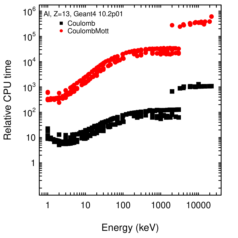
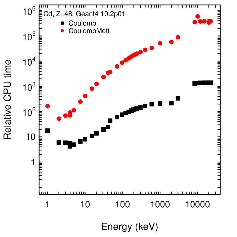
Figure 4: Ratio of average CPU time per event for configurations including G4eCoulombScatteringModel (Coulomb, black squares) and G4eSingleCoulombScatteringModel (CoulombMott, red circles), with respect to the configuration including G4EmStandardPhysics in Geant4 10.2p01. Statistical uncertainties that are smaller than the size of the markers are not visible. As explained in the text, the plot has a qualitative character, since the characteristics of the production of the backscattering validation test are not suitable for rigorous computational performance estimates.

Figure 5: Factor of improvement of the computational performance of the CoulombMott simulation configuration for a zinc target, as a function of the primary electron energy; the plot represents the ratio of CPU time consumption with Geant4 10.2p01 and with an improved version of the G4eSingleCoulombScattering model in Geant4 10.2p02.

III-E Predefined Electromagnetic PhysicsConstructors

The backscattering fraction simulated with different predefined electromagnetic PhysicsConstructors released in Geant4 10.2p01 is illustrated in Figs. 6 and 7 for a set of target elements, along with experimental measurements. Complementary information regarding the associated computational performance can be found in Figs. 8 and 9. Both figures show the ratio of CPU time with respect to simulations with the EmStd configuration; Fig. 8 concerns the EmGS, EmLivermore, EmSS and EmWVI configurations, while Fig. 9 concerns the four EmOpt1-EmOpt4 options available as variants of the G4EmStandardPhysics predefined PhysicsConstructor.

III-E1 Compatibility with experiment

Differences across the simulation results associated with predefined PhysicsConstructors and with respect to experimental data are qualitatively visible in Figs. 6 and 7; they have been quantitatively investigated adopting a similar approach to the analysis of the Goudsmit-Saunderson multiple scattering model.

For each energy range, the configuration based on the predefined PhysicsConstructor that exhibits the highest efficiency is taken as a reference, and its performance in terms of compatibility with experiment is compared with the outcome of the Anderson-Darling test deriving from other configurations. This analysis ascertains whether the predefined electromagnetic settings distributed with Geant4 produce significantly different compatibility with measurements; nevertheless, it is worhtwhile to note that at lower energies the efficiencies obtained even with most efficient predefined PhysicsContructors are substantially lower than those achieved above 100 keV.

The EmStd, EmSS and EmGS configurations, based on the G4EmStandardPhysics, G4EmStandardPhysicsSS and G4EmStandardPhysicsGS predefined PhysicsConstructors, achieve the highest efficiency among the simulations that use predefined PhysicsConstructors above 100 keV, in the 20-100 keV range and below 20 keV, respectively. Their capability to reproduce experimental data is compared with that of other simulation configurations; the resulting p-values are summarized in Table IX.

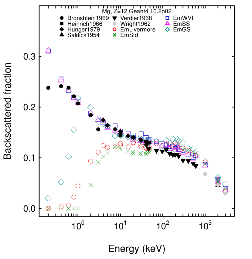
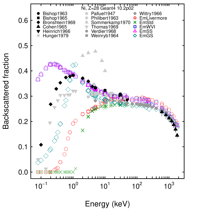
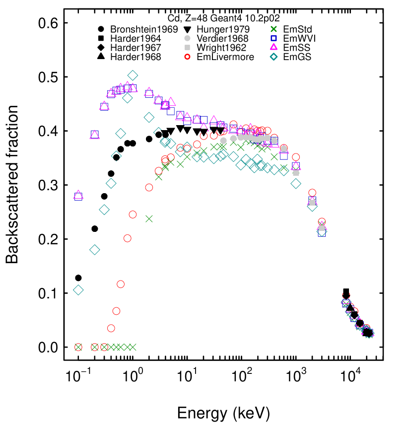
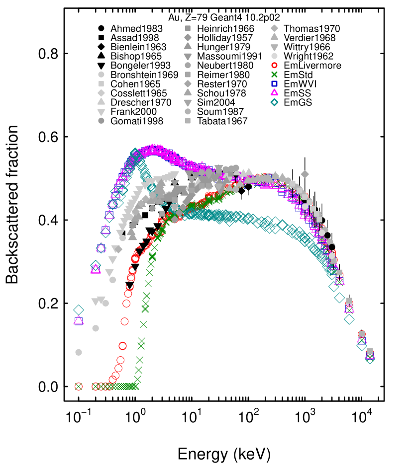
Figure 6: Measured and simulated fraction of backscattered electrons produced with different predefined PhysicsConstructors: experimental data (black and grey filled markers); simulation with Geant4 10.2p02 G4EmStandardPhysics (EmStd, green crosses), G4EmStandardPhysicsGS (EmGS turquoise empty diamonds), G4EmStandardPhysicsSS (blue empty squares), G4EmStandardPhysicsWVI (magenta empty triangles), G4EmLivermorePhysics (red empty circles). The plots concern magnesium, nickel, cadmium and gold targets.

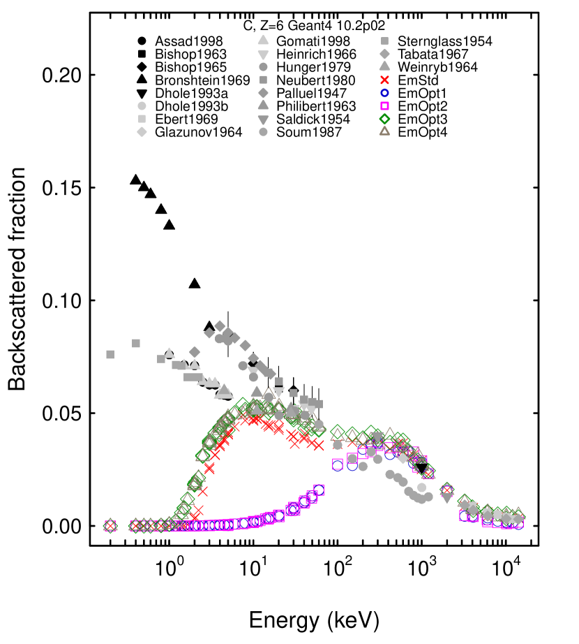
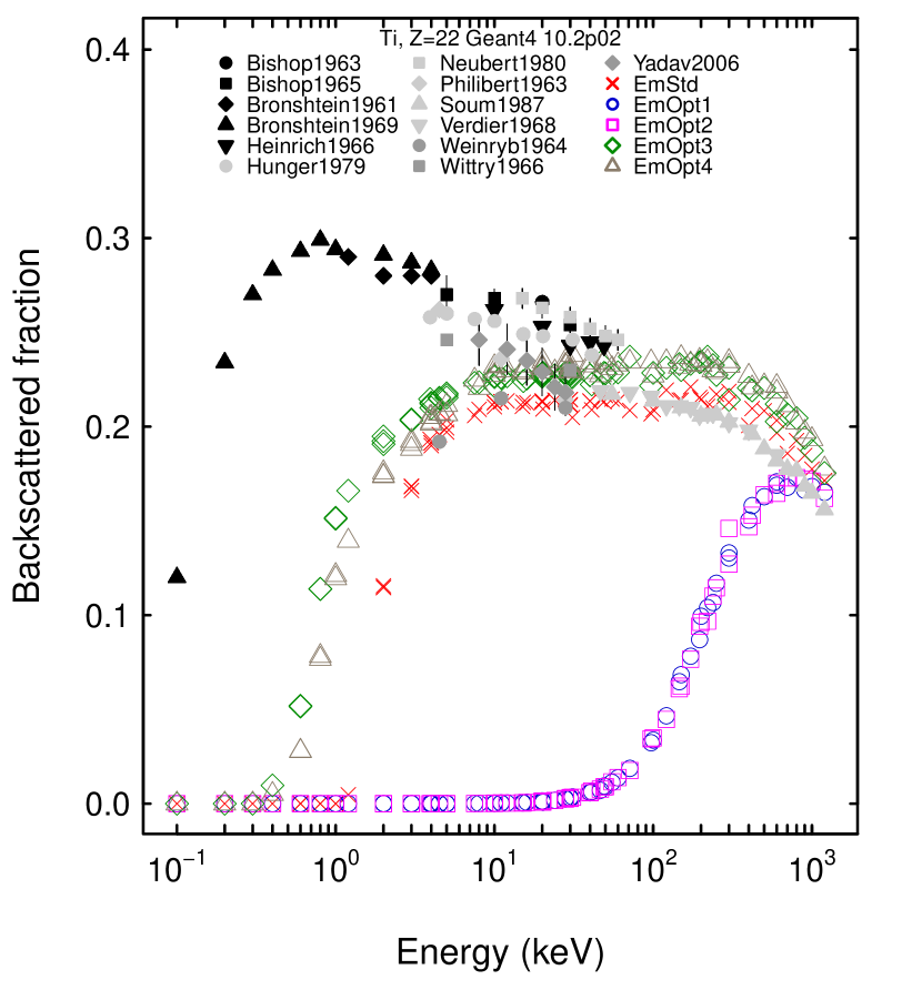
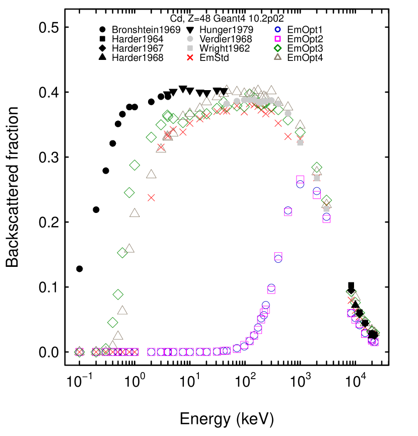
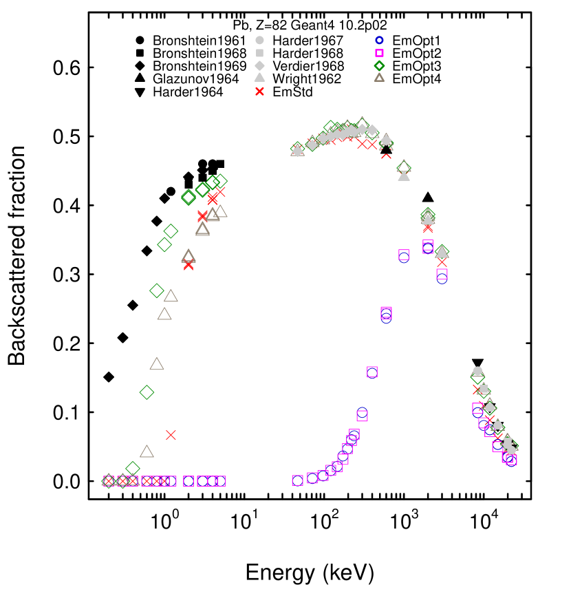
Figure 7: Measured and simulated fraction of backscattered electrons produced with different predefined electromagnetic PhysicsConstructors: experimental data (black and grey filled markers); simulation with Geant4 10.2p02 G4EmStandardPhysics (EmStd, red crosses), G4EmStandardPhysics_option1 (blue empty circles), G4EmStandardPhysics_option2 (magenta empty squares), G4EmStandardPhysics_option3 (green empty diamonds), G4EmStandardPhysics_option4 (brown empty triangles). The plots concern carbon, titanium, cadmium and lead targets.

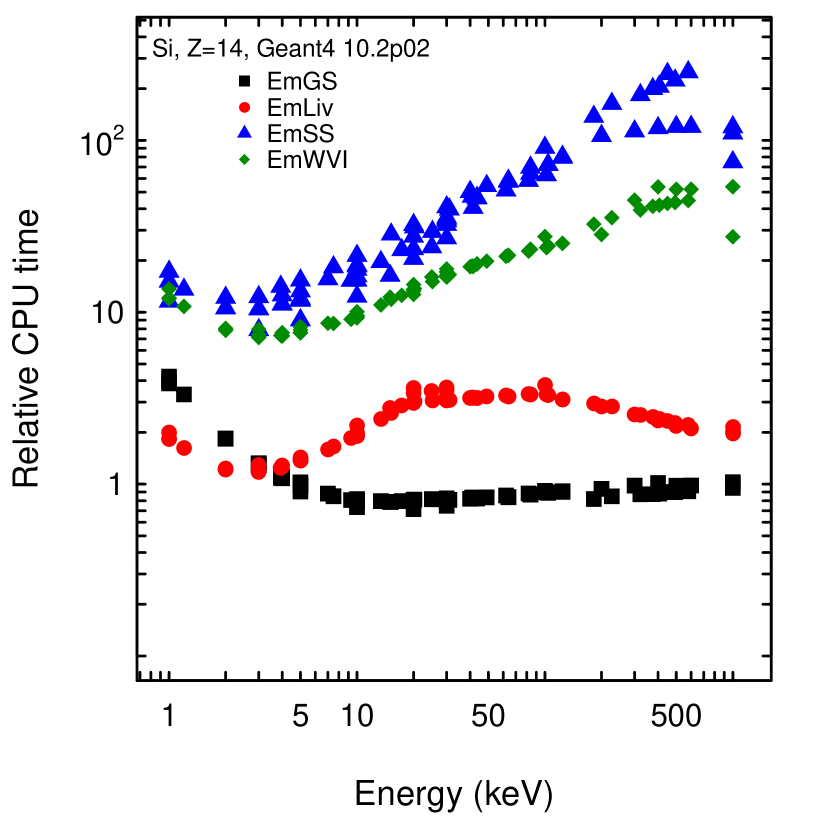
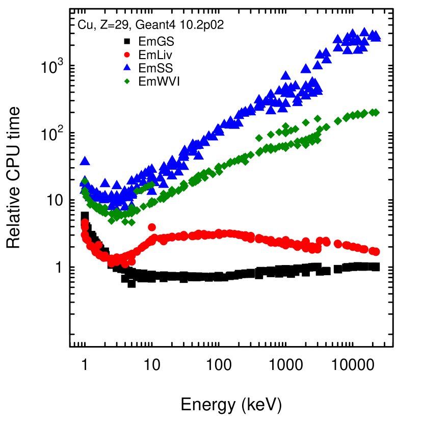
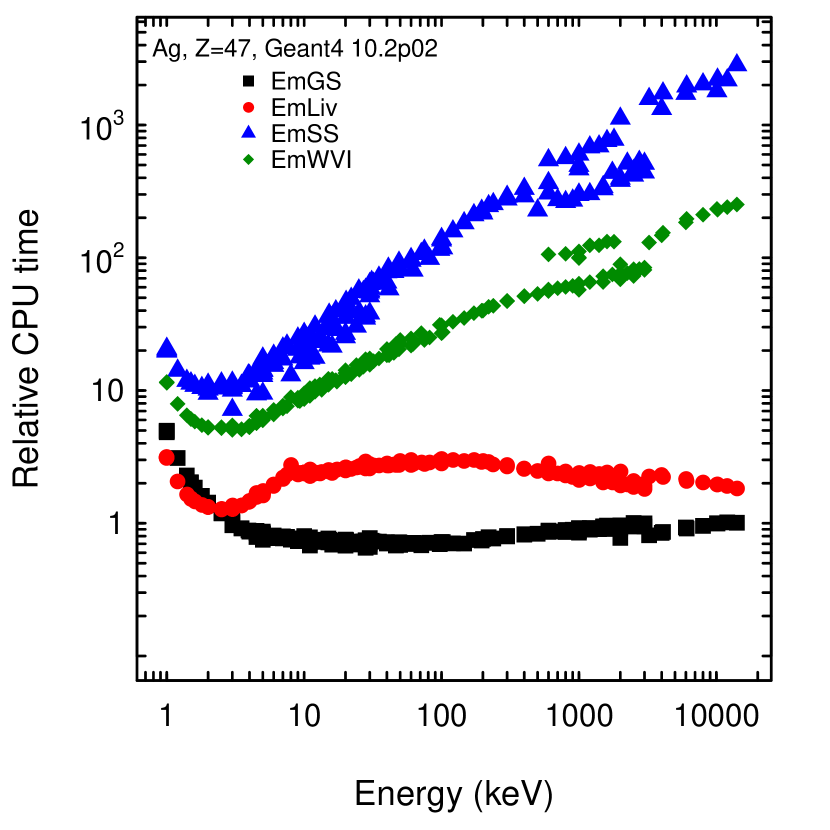
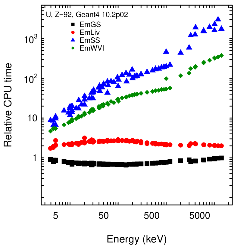
Figure 8: Computational performance of simulation configurations including predefined electromagnetic PhysicsConstructors, in test cases involving silicon, copper, silver and uranium targets: the plots report the ratio of average CPU time per event for configurations including , with respect to the configuration including G4EmStandardPhysics. The simulation were performed with Geant4 10.2p02. Statistical uncertainties are smaller than the size of the markers, if they are not visible. As explained in the text, the plot has a qualitative character, since the characteristics of the production of the backscattering validation test are not suitable for rigorous computational performance estimates.

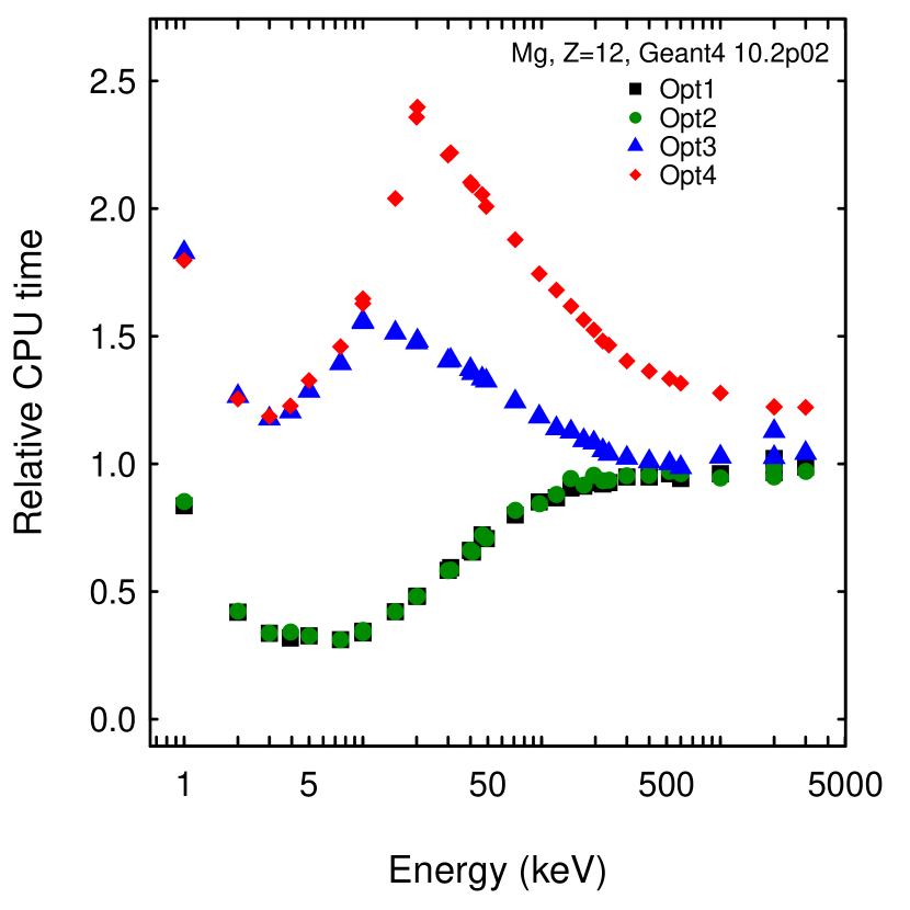
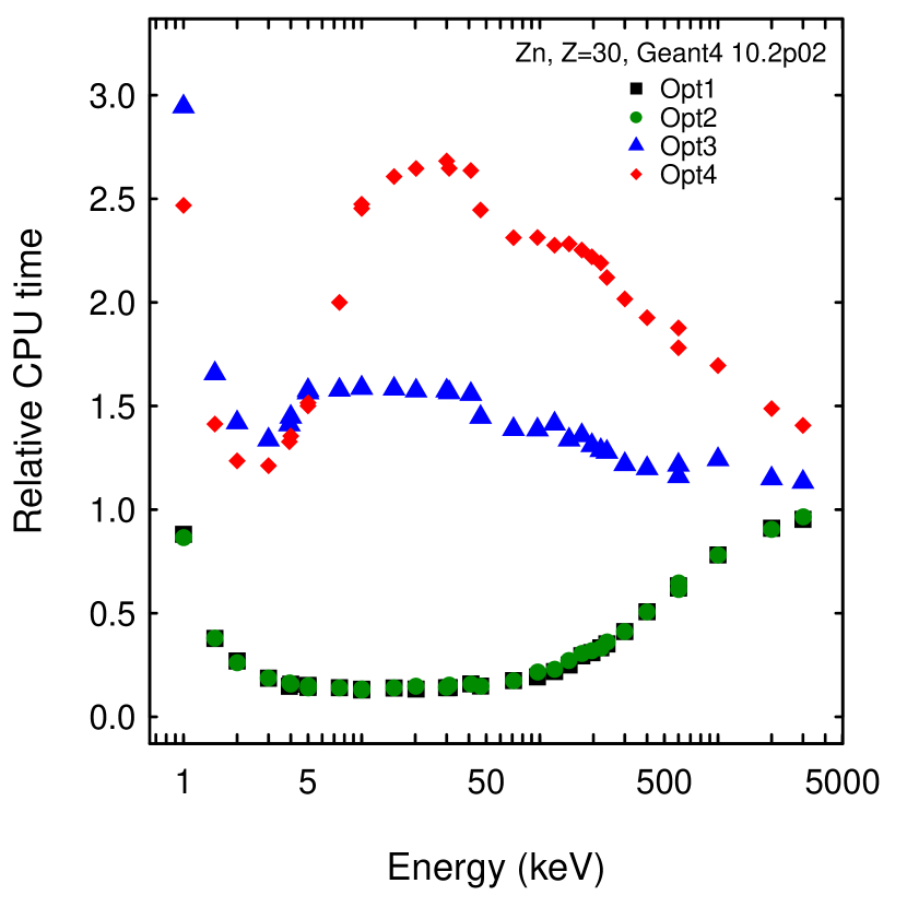
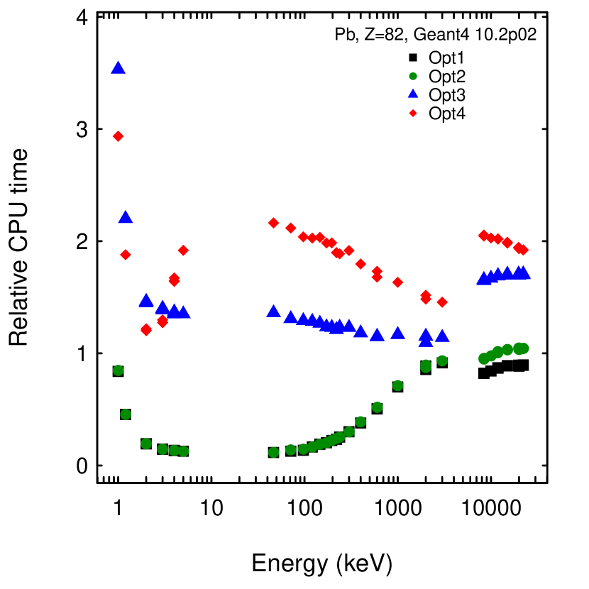
Figure 9: Computational performance of simulation configurations including predefined electromagnetic PhysicsConstructors, in test cases involving magnesium, zinc, tin and lead targets: the plots report the ratio of average CPU time per event for configurations including G4EmStandardPhysics_option1 (EmOpt1, black squares), G4EmStandardPhysics_option2 (EmOpt2, green circles), G4EmStandardPhysics_option3 (EmOpt3, blue triangles) and G4EmStandardPhysics_option4 (EmOpt4, red diamonds), with respect to the configuration including G4EmStandardPhysics. The simulation were performed with Geant4 10.2p02. Statistical uncertainties that are smaller than the size of the markers are not visible. As explained in the text, the plot has a qualitative character, since the characteristics of the production of the backscattering validation test are not suitable for rigorous computational performance estimates.

As documented in Table IX, the hypothesis of equivalent compatibility with experiment with respect to the most efficient PhysicsConstructor is rejected for any other predefined PhysicsConstructors below 20 keV, while it is rejected for all but G4StandardPhysicsWVI between 20 keV and 100 keV. Above 100 keV, the hypothesis of compatibility with experiment equivalent to that achieved with G4EmStandardPhysics is not rejected for the G4EmStandardPhysics_option3, G4EmStandardPhysics_option4, G4EmStandardPhysicsWVI and G4EmStandardPhysicsSS predefined PhysicsConstructors.

Equivalent compatibility with experiment with respect to the most efficient PhysicsConstructor is also achieved with user-defined physics configurations: at higher energy using single scattering or the WentzelVI multiple scattering model, in the intermediate energy range with the UrbanBRF and WentzelBRFP configurations, with some configuration options associated with the Goudsmit-Saunderson multiple scattering model and with the Coulomb configuration, which uses the G4eCoulombScatteringModel single scattering model.

Neither G4EmStandardPhysics_option3 nor G4EmStandardPhysics_option4, which are recommended in [16] “for simulation with high accuracy”, ensure the highest achievable accuracy of the observable in all Geant4-based simulation scenarios evaluated in this validation test.

The simulation configuration involving the G4EmLivermorePhysics PhysicsConstructor, which uses physics models encompassed in the Geant4 “low energy” electromagnetic package, does not achieve equivalent compatibility with experiment in the low energy range with respect to the more efficient configurations that use G4EmStandardPhysicsGS below 20 keV and G4EmStandardPhysicsSS or G4EmStandardPhysicsWVI between 20 and 100 keV. The hypothesis of equivalent compatibility with experiment is also rejected above 100 keV with respect to simulations performed with G4EmStandardPhysics.

The G4EmStandardPhysicsGS PhysicsConstructor achieves the highest efficiency among the predefined physics configurations examined in this test below 20 keV. The results documented in section III-C show that above 20 keV better consistency with backscattering measurements can be achieved with configurations using the Goudsmit-Saunderson multiple scattering model with settings other than those implemented in the recommended G4EmStandardPhysicsGS PhysicsConstructor, as well as with G4EmStandardPhysicsSS, G4EmStandardPhysicsWVI up to 100 keV and G4EmStandardPhysics above 100 keV.

Some broad conclusions can be drawn from the outcome of this analysis. As a general result, one can infer that no predefined PhysicsConstructor can achieve compatibility with experiment equivalent to the most efficient physics configuration across the whole energy range covered by this validation test. Additionally, predefined PhysicsConstructors explicitly labeled for “high accuracy” do not always ensure better compatibility with experimental data than other available alternatives, nor does a PhysicsConstructor using models from the Geant4 “low energy” electromagnetic package necessarily guarantee better consistency with low energy measurements.

The results of this test offer guidance to simulation users to optimize the selection of a predefined PhysicsConstructor appropriate to the characteristics of their experimental scenarios.

III-E2 Computational performance

Qualitative indications about the computational performance associated with the predefined electromagnetic PhysicsConstructors can be derived from the plots in Figs. 8 and 9.

Simulations with G4EmStandardPhysicsSS and G4EmStandardPhysicsWVI are substantially slower than those with other predefined PhysicsConstructors; Geant4 users concerned with limited availability of computational resources may want to consider user-defined physics configurations in the 20-100 keV energy range, taking into account the results of compatibility with experiment listed in Table IX as guidance to investigate appropriate settings for their own experimental scenarios.

Simulations with G4EmStandardPhysicsGS appear to be faster than with G4EmStandardPhysics above a few keV, while simulations with G4EmLivermorePhysics are generally slower; nevertheless, the difference in computational performance with respect to G4EmStandardPhysics appear to be relatively small above a few MeV. Similarly, the differences in computational speed observed with the generally slower G4EmStandardPhysics_option3, G4EmStandardPhysics_option4 and with the generally faster G4EmStandardPhysics_option1, G4EmStandardPhysics_option2 options tend to decrease at higher energies.

III-E3 Energy Deposition

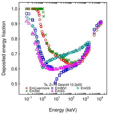
Figure 10: Fraction of the primary electron energy deposited in a tantalum target as a function of the primary electron energy: G4EmStandardPhysics (EmStd, green crosses), G4EmStandardPhysicsGS (EmGS, turquoise downward triangles), G4EmStandardPhysicsSS (EmSS, magenta upward triangles), G4EmStandardPhysicsWVI (EmWVI, blue squares) and G4EmLivermorePhysics (EmLiv, red circles). This plot has a qualitative character to illustrate the effects of different modeling options on the simulation of energy deposition in a volume.

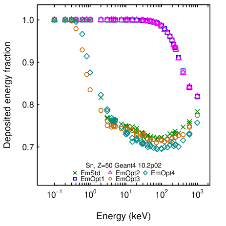
Figure 11: Fraction of the primary electron energy deposited in a tin target as a function of the primary electron energy: G4EmStandardPhysics (EmStd, green crosses), G4EmStandardPhysics_option1 (EmOpt1, blue squares), G4EmStandardPhysics_option2 (EmOpt2, magenta upward triangles), G4EmStandardPhysics_option3 (EmOpt3, turquoise downward triangles and G4EmStandardPhysics_option4 (EmOpt4, brown diamonds). This plot has a qualitative character to illustrate the effects of different electron scattering options on the simulation of energy deposition in a volume.

The simulation of the energy deposited in a volume is affected by the accuracy of the simulation of electron scattering. In this respect, one should take into account that electrons can be either primary or secondary particles.

A detailed analysis of the effects of different options for electron scattering modeling on the simulation of deposited energy is outside the scope of this paper; moreover, the simple experimental model of backscattering experiments considered in this test would not be adequate for in-depth studies of energy deposition simulation with Geant4. Nevertheless, an example of the effects of different predefined PhysicsConstructors is illustrated in Figs. 10 and 11 for a qualitative appraisal. The plots, based on Geant4 10.2p02, show the fraction of the primary electron energy that is deposited in the targets modeled in this backscattering validation test: differences are visible in the energy deposited in the target associated with the various predefined physics options.

IV Epistemological Considerations

Some epistemological guidelines should be taken into account in the appraisal of the results documented in this paper, as well as in similar contexts of validation tests concerning observables produced in use cases of Monte Carlo simulation codes.

Although the observable considered in this validation test is sensitive to electron scattering modeling, its simulated outcome is the result of all the code involved in the simulation, including direct and indirect dependencies, and of the computational environment where the simulation is produced. The simulation configurations studied in this paper are identified for convenience through the electron scattering modeling they involve, nevertheless possible effects of other parts of the simulation code on shaping the observable subject to validation should not be neglected. This limitation of inference is common to any observable produced as a result of a Monte Carlo simulation system. In this respect, a validation test specific to a simulation use case is epistemologically distinct from the context of the validation of parameters used in Monte Carlo codes, e.g. cross sections, which can be compared with experimental measurements independently from the Monte Carlo software systems where they are used.

It is worthwhile to remind the reader that all the results associated with the simulation configurations considered in this paper concern the test of a specific observable, i.e. the fraction of backscattered electrons. Caution should be exercised in extrapolating them to assess the reliability of other simulated observables not subject to validation in this paper, or to other physically different environments, e.g. at lower or higher energies [41].

Known concerns related to the role of induction in establishing scientific knowledge [42], which question the foundation of general statements about the validity or the accuracy of simulation models, should be taken into account. A correct approach consists of documenting the context in which the behaviour of models has been empirically quantified.

V Conclusion

The results collected in this paper document validation tests of Geant4-based simulation of electron backscattering with a wide variety of physics modelling options available in the Geant4 toolkit. Statistical data analysis methods allow quantitative and objective appraisal of the capabilities of different physics configurations to produce simulation results compatible with experimental measurements.

Significant differences are observed across the set of physics options subject to test, regarding their ability to generate results consistent with the measured fraction of backscattered electrons. No single physics modeling configuration is capable of producing optimal results over the whole energy range covered by the validation test. The detailed validation analysis summarized in this paper provides guidance to help experimental users identify, among the many possible options available in the toolkit, those that most effectively address the requirements specific to their own experimental scenarios. Comparative evaluations of the computational performance of the simulation configurations, documented along with the results of validation tests, provide complementary information, although at a qualitative level, to guide the selection.

The results collected in this paper show the benefit of validation tests of simulation modeling options, whose capabilities are quantified with respect to large experimental data samples through statistical analysis methods. Their inclusion in the software development process of simulation toolkits is beneficial to the experimental community, both to support the optimization of new models in the course of their development and to provide users with an objective characterization of the behaviour of the software released for scientific applications.

References

- [1] S. Agostinelli et al., “Geant4 - a simulation toolkit”, Nucl. Instrum. Meth. A, vol. 506, no. 3, pp. 250-303, 2003.
- [2] J. Allison et al., “Geant4 Developments and Applications” , IEEE Trans. Nucl. Sci., vol. 53, no. 1, pp. 270-278, 2006.
- [3] S. H. Kim et al., “Validation test of Geant4 simulation of electron backscattering”, IEEE Trans. Nucl. Sci., vol. 62, no. 2, pp. 451-479, 2015.
- [4] T. Basaglia et al., “Investigation of Geant4 Simulation of Electron Backscattering”, IEEE Trans. Nucl. Sci., vol. 62, no. 4, pp. 1805-1812, 2015.
- [5] S. Goudsmit and J. L. Saunderson, “Multiple Scattering of Electrons”, Phys. Rev., vol. 58, pp. 24-29, 1940.
- [6] S. Goudsmit and J. L. Saunderson, “Multiple Scattering of Electrons. II”, Phys. Rev., vol. 58, pp. 36-42, 1940.
- [7] N. F. Mott, “The scattering of fast electrons by atomic nuclei”, Proc. Roy. Soc. A, vol. 124, pp. 425-442, 1929.
- [8] N. F. Mott, “The Polarization of Electrons by Double Scattering”, Proc. Roy. Soc. A, vol. 135, pp. 429-458, 1932.
- [9] M. J. Boschini et al., “An expression for the Mott cross section of electrons and positrons on nuclei with Z up to 118”, Radiat. Phys. Chem., vol. 90, pp. 39-66, 2013.
- [10] E. Ronchieri, M. G. Pia and F. Giacomini, “First statistical analysis of Geant4 quality software metrics”, J. Phys. Conf. Series, vol. 664, p. 062053, 2015.
- [11] S. T. Perkins, D. E. Cullen, and S. M. Seltzer, “Tables and Graphs of Electron-Interaction Cross Sections from 10 eV to 100 GeV Derived from the LLNL Evaluated Electron Data Library (EEDL)”, UCRL-50400 Vol. 31, 1997.
- [12] D. Cullen et al., “EPDL97, the Evaluated Photon Data Library”, Lawrence Livermore National Laboratory Report UCRL-50400, Vol. 6, Rev. 5, 1997.
- [13] J. Apostolakis, S. Giani, M. Maire, P. Nieminen, M.G. Pia, L. Urban, “Geant4 low energy electromagnetic models for electrons and photons” INFN/AE-99/18, Frascati, 1999.
- [14] S. Chauvie, G. Depaola, V. Ivanchenko, F. Longo, P. Nieminen and M. G. Pia, “Geant4 Low Energy Electromagnetic Physics”, in Proc. Computing in High Energy and Nuclear Physics, Beijing, China, pp. 337-340, 2001.
- [15] S. Chauvie et al., “Geant4 Low Energy Electromagnetic Physics”, in 2004 IEEE Nucl. Sci. Symp. Conf. Rec., pp. 1881-1885, 2004.
- [16] Geant4 10.2, “User’s Guide: For Application Developers” [Online]. Available: http://geant4.web.cern.ch/geant4/UserDocumentation/UsersGuides/ForApplicationDeveloper/html/index.html.
- [17] L. Urban, “A Model for multiple scattering in Geant4”, in Proc. of The Monte Carlo Method: Versatility Unbounded in a Dynamic Computing World, on CD-ROM, American Nuclear Society, La Grange Park, IL, 2005.
- [18] L. Urban, “A model of multiple scattering in Geant4”, CERN-OPEN-2006-077, Geneva, Switzerland, 2006.
- [19] I. Kawrakow, E. Mainegra-Hing, D.W.O. Rogers, F. Tessier and B. R. B. Walters, “The EGSnrc Code System: Monte Carlo Simulation of Electron and Photon Transport”, NRCC PIRS-701 Report, 6th printing, National Research Council of Canada, Ottawa, Canada, 2013.
- [20] Geant4 10.2, “Geant4 Physics Reference Manual, version 10.2”, [Online]. Available: http://geant4.web.cern.ch/geant4/UserDocumentation/UsersGuides/PhysicsReferenceManual/fo/PhysicsReferenceManual.pdf.
- [21] G. A. P. Cirrone et al., “A Goodness-of-Fit Statistical Toolkit”, IEEE Trans. Nucl. Sci., vol. 51, no. 5, pp. 2056-2063, 2004.
- [22] B. Mascialino, A. Pfeiffer, M. G. Pia, A. Ribon, and P. Viarengo, “New developments of the Goodness-of-Fit Statistical Toolkit”, IEEE Trans. Nucl. Sci., vol. 53, no. 6, pp. 3834-3841, 2006.
- [23] R Core Team, “R: A language and environment for statistical computing” R Foundation for Statistical Computing, Vienna, Austria, ISBN 3-900051-07-0, 2012. [Online]. Available: http://www.R-project.org/.
- [24] M. Paterno, “Calculating Efficiencies and Their Uncertainties”, Fermi National Accelerator Report FERMILAB-TM-2286-CD, Batavia, IL, 2004.
- [25] A. G. Frodesen, O. Skjeggestad, and H. Tøfte, “Probability and statistics in particle physics”, Ed. Universitetsforlaget, Bergen, 1979.
- [26] T. W. Anderson and D. A. Darling, “Asymptotic theory of certain goodness of fit criteria based on stochastic processes”, Ann. Math. Stat., vol. 23, pp. 193-212, 1952.
- [27] T. W. Anderson and D. A. Darling, “A test of goodness of fit”, J. Am. Stat. Ass., vol. 49, pp. 765-769, 1954.
- [28] H. Cramér, “On the composition of elementary errors. Second paper: statistical applications”, Skand. Aktuarietidskr., vol. 11, pp. 13-74, pp. 141-180, 1928.
- [29] R. von Mises, Wahrscheinlichkeitsrechnung und ihre Anwendung in der Statistik und theoretischen Physik, Leipzig: F. Duticke, 1931.
- [30] A. N. Kolmogorov, “Sulla determinazione empirica di una legge di distribuzione”, Gior. Ist. Ital. Attuari, vol. 4, pp. 83-91, 1933.
- [31] N. V. Smirnov, “On the estimation of the discrepancy between empirical curves of distributions for two independent samples”, Bull. Math. Univ. Moscow, 1939.
- [32] G. S. Watson, “Goodness-of-fit tests on a circle”, Biometrika, vol. 48, pp. 109-114, 1961.
- [33] R. A. Fisher, “On the interpretation of from contingency tables, and the calculation of P”, J. Royal Stat. Soc., vol. 85, no. 1, pp. 87-94, 1922.
- [34] G. A. Barnard, “ Significance tests for 2 × 2 tables”, Biometrika, vol. 34, pp. 123-138, 1947.
- [35] S. Suissa, and J. J. Shuster, “Exact Unconditional Sample Sizes for the 22 Binomial Trial”, J. Royal Stati. Soc., Ser. A, vol. 148, pp. 317-327, 1985.
- [36] R. D. Boschloo, “Raised Conditional Level of Significance for the 22-table when Testing the Equality of Two Probabilities”, Stat. Neerlandica, vol. 24, pp. 1-35, 1970.
- [37] K. Pearson, “On the test of Goodness of Fit”, Biometrika, vol. 14, no. 1-2, pp. 186-191, 1922.
- [38] A. Agresti, “A Survey of Exact Inference for Contingency Tables”, Stat. Sci., vol. 7, pp. 131-153, 1992.
- [39] A. Martin Andres and A. Silva Mato, “Choosing the optimal unconditioned test for comparing two independent proportions”, Comp. Stat. Data Anal., vol. 17, pp. 555-574, 1994.
- [40] A. Martin Andres, A. Silva Mato, J. M . Tapia Garcia, and M. J. Sanchez Quevedo, “Comparing the asymptotic power of exact tests in 2 × 2 tables”, Comp. Stat. Data Anal., vol. 47, pp. 745-756, 2004.
- [41] W. L. Oberkampf, M. Pilch, and T. G. Trucano, “Predictive Capability Maturity Model for Computational Modeling and Simulation”, Sandia National Laboratories Report, SAND2007-5948, Albuquerque, NM, USA, 2007.
- [42] K. Popper, “Der Logik der Forschung”, Vienna: J. Springer, 1935.