Approximate Partial Order Reduction

Abstract

We present a new partial order reduction method for reachability analysis of nondeterministic labeled transition systems over metric spaces. Nondeterminism arises from both the choice of the initial state and the choice of actions, and the number of executions to be explored grows exponentially with their length. We introduce a notion of $\varepsilon$-independence relation over actions that relates approximately commutative actions; $\varepsilon$-equivalent action sequences are obtained by swapping $\varepsilon$-independent consecutive action pairs. Our reachability algorithm generalizes individual executions to cover sets of executions that start from different, but $\delta$-close initial states, and follow different, but $\varepsilon$-independent, action sequences. The constructed over-approximations can be made arbitrarily precise by reducing the $\delta,\varepsilon$ parameters. Exploiting both the continuity of actions and their approximate independence, the algorithm can yield an exponential reduction in the number of executions explored. We illustrate this with experiments on consensus, platooning, and distributed control examples.

1 Introduction

Actions of different computing nodes interleave arbitrarily in distributed systems. The number of action sequences that have to be examined for state-space exploration grows exponentially with the number of nodes. Partial order reduction methods tackle this combinatorial explosion by eliminating executions that are equivalent, i.e., do not provide new information about reachable states  (see [19, 27, 22] and the references therein). This equivalence is based on independence of actions: a pair of actions are independent if they commute, i.e., applying them in any order results in the same state. Thus, of all execution branches that start and end at the same state, but perform commuting actions in different order, only one has to be explored. Partial order reduction methods have become standard tools for practical software verification. They have been successfully applied to election protocols [2], indexers [18], file systems [9], security protocol [8], distributed schedulers [3], among many others.

Current partial order methods are limited when it comes to computation with numerical data and physical quantities (e.g., sensor networks, vehicle platoons, IoT applications, and distributed control and monitoring systems). First, a pair of actions are considered independent only if they commute exactly; actions that nearly commute—as are common in these applications—cannot be exploited for pruning the exploration. Second, conventional partial order methods do not eliminate executions that start from nearly similar states and experience equivalent action sequences.

We address these limitations and propose a state space exploration method for nondeterministic, infinite state transition systems based on approximate partial order reduction. Our setup has two mild assumptions: (i) the state space of the transition system has a discrete part $L$ and a continuous part $X$ and the latter is equipped with a metric; (ii) the actions on $X$ are continuous functions. Nondeterminism arises from both the choice of the initial state and the choice of actions. Fixing an initial state $q_{0}$ and a sequence of actions $\tau$ (also called a trace), uniquely defines an execution of the system which we denote by $\xi_{q_{0},\tau}$. For a given approximation parameter $\varepsilon\geq 0$, we define two actions $a$ and $b$ to be $\varepsilon$-independent if from any state $q$, the continuous parts of states resulting from applying action sequences $ab$ and $ba$ are $\varepsilon$-close. Two traces of ${\cal A}$ are $\varepsilon$-equivalent if they result from permuting $\varepsilon$-independent actions. To compute the reachable states of ${\cal A}$ using a finite (small) number of executions, the key is to generalize or expand an execution $\xi_{q_{0},\tau}$ by a factor $r\geq 0$, so that, this expanded set contains all executions that start $\delta$-close to $q_{0}$ and experience action sequences that are $\varepsilon$-equivalent to $\tau$. We call this $r$ a $(\delta,\varepsilon)$-trace equivalent discrepancy factor ($\mathit{ted}$) for $\xi$.

For a fixed trace $\tau$, the only source of nondeterminism is the choice of the initial state. The reachable states from $B_{\delta}(q_{0})$—a $\delta$-ball around $q_{0}$—can be over-approximated by expanding $\xi_{q_{0},\tau}$ by a $(\delta,0)$-$\mathit{ted}$. This is essentially the sensitivity of $\xi_{q_{0},\tau}$ to $q_{0}$. Techniques for computing it are now well-developed for a broad class of models  [13, 11, 14, 15].

Fixing $q_{0}$, the only source of nondeterminism is the possible sequence of actions in $\tau$. The reachable states from $q_{0}$ following all possible valid traces can be over-approximated by expanding $\xi_{q_{0},\tau}$ by a $(0,\varepsilon)$-$\mathit{ted}$, which includes states reachable by all $\varepsilon$-equivalent action sequences. Computing $(0,\varepsilon)$-$\mathit{ted}$ uses the principles of partial order reduction. However, unlike exact equivalence, here, starting from the same state, the states reached at the end of executing two $\varepsilon$-equivalent traces are not necessarily identical. This breaks a key assumption necessary for conventional partial order algorithms: here, an action enabled after $ab$ may not be enabled after $ba$. Of course, considering disabled actions can still give over-approximation of reachable states, but, we show that the precision of approximation can be improved arbitrarily by shrinking $\delta$ and $\varepsilon$.

Thus, the reachability analysis in this paper brings together two different ideas for handling nondeterminism: it combines sensitivity analysis with respect to initial state and $\varepsilon$-independence of actions in computing $(\delta,\varepsilon)$-$\mathit{ted}$, i.e., upper-bounds on the distance between executions starting from initial states that are $\delta$-close to each other and follow $\varepsilon$-equivalent action sequences (Theorem 5.1). As a matter of theoretical interest, we show that the approximation error can be made arbitrarily small by choosing sufficiently small $\delta$ and $\varepsilon$ (Theorem 5.2). We validate the correctness and effectiveness of the algorithm with three case studies where conventional partial order reduction would not help: an iterative consensus protocol, a simple vehicle platoon control system, and a distributed building heating system. In most cases, our reachability algorithm reduces the number of explored executions by a factor of $O(n!)$, for a time horizon of $n$, compared with exhaustive enumeration. Using these over-approximations, we could quickly decide safety verification questions. These examples illustrate that our method has the potential to improve verification of a broader range of distributed systems for consensus [5, 16, 26, 25], synchronization [30, 28] and control [17, 24].

Related work.

There are two main classes of partial order reduction methods. The persistent/ample set methods compute a subset of enabled transitions –the persistent set (or ample set)– such that the omitted transitions are independent to those selected [10, 2]. The reduced system which only considers the transitions in the persistent set is guaranteed to represent all behaviors of the original system. The persistent sets and the reduced systems are often derived by static analysis of the code. More recently, researchers have developed dynamic partial order reduction methods using the sleep set to avoid the static analysis [31, 1, 18]. These methods examine the history of actions taken by an execution and decide a set of actions that need to be explored in the future. The set of omitted actions is the sleep set. In [6], Cassez and Ziegler introduce a method to apply symbolic partial order reduction to infinite state discrete systems.

Analysis of sensitivity and the related notion of robustness analysis functions, automata, and executions has recently received significant attention [7, 11, 29]. Majumdar and Saha [23] present an algorithm to compute the output deviation with bounded disturbance combining symbolic execution and optimization. In [7] and [29], Chaudhuri etc., present algorithms for robustness analysis of programs and networked systems. Automatic techniques for local sensitivity analysis combining simulations and static analysis and their applications to verification of hybrid systems have been presented in [11, 14, 15].

In this paper, instead of conducting conventional partial order reduction, we propose a novel method of approximate partial order reduction, and combine it with sensitivity analysis for reachability analysis and safety verification for a broader class of systems.

2 Preliminaries

Notations.

The state of our labeled transition system is defined by the valuations of a set of variables. Each variable $v$ has a type, $\mathit{type}(v)$, which is either the set of reals or some finite set. For a set of variables $V$, a valuation ${\bf v}$ maps each $v\in V$ to a point in $\mathit{type}(v)$. The set of all valuations of $V$ is ${\mbox{\it Val}}(V)$. ${\mathbb{R}}$ denotes the set of reals, ${{\mathbb{R}}_{\geq 0}}$ the set of non-negative reals, and ${\mathbb{N}}$ the set of natural numbers. For $n\in{\mathbb{N}}$, $[n]=\{0,\ldots,n-1\}$. The spectral radius $\rho(A)$ of a square matrix $A\in{\mathbb{R}}^{n\times n}$ is the largest absolute value of its eigenvalues. A square matrix $A$ is stable if its spectral radius $\rho(A)<1$. For a set of tuples $S=\{\langle s_{j1},\dots,s_{jn}\rangle_{j}\}$, $S\mathrel{\lceil}i$ denotes the set $\{s_{ji}\}$ which is the set obtained by taking the $i^{th}$ component of each tuple in $S$.

2.1 Transition systems

Definition 1

A labeled transition system ${\cal A}$ is a tuple $\langle X\cup L,\Theta,A,\mathrel{\stackrel{{\scriptstyle}}{{\rightarrow}}}\rangle$ where (i) $X$is a set of real-valued variables and $L$ is a set of finite-valued variables. $Q={\mbox{\it Val}}(X\cup L)$ is the set of states, (ii) $\Theta\subseteq Q$is a set of initial states such that the sets of real-valued variables are compact, (iii) $A$is a finite set of actions, and (iv) $\rightarrow\subseteq Q\times A\times Q$is a transition relation.

A state $q\in Q$ is a valuation of the real-valued and finite-valued variables. We denote by $q.X$ and $q.L$, respectively, the real-valued and discrete (finite-valued) parts of the state $q$. We will view the continuous part $q.X$ as a vector in ${\mathbb{R}}^{|X|}$ by fixing an arbitrary ordering of $X$. The norm $|\cdot|$ on $q.X$ is an arbitrary norm unless stated otherwise. For $\delta\geq 0$, the $\delta$-neighborhood of $q$ is denoted by ${\cal B}_{\delta}(q)\mathrel{\stackrel{{\scriptstyle\scriptscriptstyle\Delta}}{{=}}}\{q^{\prime}\in Q:q^{\prime}.L=q.L\wedge|q^{\prime}.X-q.X|\leq\delta\}$. For any $(q,a,q^{\prime})\in\mathrel{\stackrel{{\scriptstyle}}{{\rightarrow}}}$, we write $q\mathrel{\stackrel{{\scriptstyle a}}{{\rightarrow}}}q^{\prime}$. For any action $a\in A$, its guard is the set $\mathit{guard}(a)=\{q\in Q\ |\ \exists q^{\prime}\in Q,q\mathrel{\stackrel{{\scriptstyle a}}{{\rightarrow}}}q^{\prime}\}$. We assume that guards are closed sets. An action $a$ is deterministic if for any state $q\in Q$, if there exists $q_{1},q_{2}\in Q$ with $q\mathrel{\stackrel{{\scriptstyle a}}{{\rightarrow}}}q_{1}$ and $q\mathrel{\stackrel{{\scriptstyle a}}{{\rightarrow}}}q_{2}$, then $q_{1}=q_{2}$.

Assumption 1

(i) Actions are deterministic. For notational convenience, the name of an action $a$ is identified with its transition function, i.e., for each $q\in\mathit{guard}(a)$, $q\mathrel{\stackrel{{\scriptstyle a}}{{\rightarrow}}}a(q)$. We extend this notation to all states, i.e., even those outside $\mathit{guard}(a)$. (ii) For any state pair $q,q^{\prime}$, if $q.L=q^{\prime}.L$ then $a(q).L=a(q^{\prime}).L$.

Executions and traces.

For a deterministic transition system, a state $q_{0}\in Q$ and a finite action sequence (also called a trace) $\tau=a_{0}a_{1}\dots a_{n-1}$ uniquely specifies a potential execution $\xi_{q_{0},\tau}=q_{0},a_{0},q_{1},a_{1},\dots,a_{n-1},q_{n}$ where for each $i\in[n],$ $a_{i}(q_{i})=q_{i+1}$. A valid execution (also called execution for brevity) is a potential execution with (i) $q_{0}\in\Theta$ and (ii) for each $i\in[n]$, $q_{i}\in\mathit{guard}(a_{i})$. That is, a valid execution is a potential execution starting from the initial set with each action $a_{i}$ enabled at state $q_{i}$. For any potential execution $\xi_{q_{0},\tau}$, its trace is the action sequence $\tau$, i.e., $\mathit{trace}(\xi_{q_{0},\tau})=\tau\in A^{*}$. We denote by $len(\tau)$ the length of $\tau$. For any for $i\in[len(\tau)]$, $\tau(i)$ is the $i$-th action in $\tau$. The length of $\xi_{q_{0},\tau}$ is the length of its trace and $\xi_{q_{0},\tau}(i)=q_{i}$ is the state visited after the $i$-th transition. The first and last state on a execution $\xi$ are denoted as $\xi.\mathop{\mathsf{fstate}}=\xi(0)$ and $\xi.\mathop{\mathsf{lstate}}=\xi(len(\xi))$.

For a subset of initial states $S\subseteq\Theta$ and a time bound $T\geq 0$, ${\sf Execs}(S,T)$ is the set of length $T$ executions starting from $S$. We denote the reach set at time $T$ by ${\sf Reach}(S,T)\mathrel{\stackrel{{\scriptstyle\scriptscriptstyle\Delta}}{{=}}}\{\xi.\mathop{\mathsf{lstate}}\ |\ \xi\in{\sf Execs}(S,T)\}$. Our goal is to precisely over-approximate ${\sf Reach}(\Theta,T)$ exploiting partial order reduction.

  ⬇ 1automaton ${\operatorname{\mathsf{Consensus}}}(n\in{\mathbb{N}},N\in{\mathbb{N}})$ variables 3 $x:{\mathbb{R}}^{n}$ $d:{\mathbb{B}}^{N}$ 5 initially $x[i]\in[-4,4]$ for each $i\in[n]$ 7 $d[i]:=\mathit{false}$ for each $i\in[n]$ ⬇ transitions 9 ${\operatorname{\mathsf{a_{i}}}}$ for each $i\in[N]$ pre $\neg d_{i}$ 11 eff $x:=A_{i}x\ \wedge\ d[i]:=\mathit{t}rue$ ${\operatorname{\mathsf{a_{\bot}}}}$ 13 pre $\wedge_{i\in[N]}d[i]$ eff $d[i]:=\mathit{false}$ for each $i\in[N]$  

Figure 1: Labeled transition system model of iterative consensus.

Example 1 (Iterative consensus)

An $n$-dimensional iterative consensus protocol with $N$ processes is shown in Figure 1. The real-valued part of state is a vector $x$ in ${\mathbb{R}}^{n}$ and each process $i$ changes the state by the linear transformation $x\leftarrow A_{i}x$. The system evolves in rounds: in each round, each process $i$ updates the state exactly once but in arbitrary order. The boolean vector $d$ marks the processes that have acted in a round. The set of actions is $\{a_{i}\}_{i\in[N]}\cup\{a_{\bot}\}$. For each $i\in[N]$, the action $a_{i}$ is enabled when $d[i]$ is $\mathit{false}$ and when it occurs $x$ is updated as $A_{i}x$, where $A_{i}$ is an $n\times n$ matrix. The action $a_{\bot}$ can occur only when all $d[i]$’s are set to $\mathit{true}$ and it resets all the $d[i]$’s to $\mathit{false}$. For an instance with $N=3$, a valid execution could have the trace $\tau=a_{0}a_{2}a_{1}a_{\bot}a_{1}a_{0}a_{2}a_{\bot}$. It can be checked that Assumption 1 holds. In fact, the assumption will continue to hold if $A_{i}x$ is replaced by a nonlinear transition function $a_{i}:{\mathbb{R}}^{n}\rightarrow{\mathbb{R}}^{n}$.

2.2 Discrepancy functions

A discrepancy function bounds the changes in a system’s executions as a continuous function of the changes in its inputs. Methods for computing discrepancy of dynamical and hybrid systems are now well-developed [21, 14, 12]. We extend the notion naturally to labeled transition systems: a discrepancy for an action bounds the changes in the continuous state brought about by its transition function.

Definition 2

For an action $a\in A$, a continuous function $\beta_{a}:{{\mathbb{R}}_{\geq 0}}\rightarrow{{\mathbb{R}}_{\geq 0}}$ is a discrepancy function if for any pair of states $q,q^{\prime}\in Q$ with $q.L=q^{\prime}.L$, (i) $|a(q).X-a(q^{\prime}).X|\leq\beta_{a}(|q.X-q^{\prime}.X|)$, and (ii) $\beta_{a}(\cdot)\rightarrow 0$as $|q.X-q^{\prime}.X|\rightarrow 0$.

Property (i) gives an upper-bound on the changes brought about by action $a$ and (ii) ensures that the bound given by $\beta_{a}$ can be made arbitrarily precise. If the action $a$ is Lipschitz continuous with Lipschitz constant $L_{a}$, then $\beta_{a}(|q.X-q^{\prime}.X|)=L_{a}(|q.X-q^{\prime}.X|)$ can be used as a discrepancy function. Note that we do not assume the system is stable. As the following proposition states, given discrepancy functions for actions, we can reason about distance between executions that share the same trace but have different initial states.

Proposition 1

Suppose each action $a\in A$ has a discrepancy function $\beta_{a}$. For any $T\geq 0$ and action sequence $\tau=a_{0}a_{1}a_{2}\dots a_{T}$, and for any pair of states $q,q^{\prime}\in Q$ with $q.L=q^{\prime}.L$, the last states of the pair of potential executions satisfy:

$$\xi_{q,\tau}.\mathop{\mathsf{lstate}}.L =\xi_{q^{\prime},\tau}.\mathop{\mathsf{lstate}}.L,$$ (1)

$$|\xi_{q,\tau}.\mathop{\mathsf{lstate}}.X-\xi_{q^{\prime},\tau}.\mathop{\mathsf{lstate}}.X| \leq\beta_{a_{T}}\beta_{a_{T-1}}\dots\beta_{a_{0}}(|q.X-q^{\prime}.X|).$$ (2)

Example 2

Consider an instance of ${\operatorname{\mathsf{Consensus}}}$ of Example 1 with $n=3$ and $N=3$ with the standard $2$-norm on ${\mathbb{R}}^{3}$. Let the matrices $A_{i}$ be

$$\scriptsize A_{0}=\begin{bmatrix}0.2&-0.2&-0.3\\ -0.2&0.2&-0.1\\ -0.3&-0.1&0.3\end{bmatrix},A_{1}=\begin{bmatrix}0.2&0.3&0.2\\ 0.3&-0.2&0.3\\ 0.2&0.3&0\end{bmatrix},A_{2}=\begin{bmatrix}-0.1&0&0.4\\ 0&0.4&-0.2\\ 0.4&-0.2&-0.1\end{bmatrix}.$$

It can be checked that for any pair $q,q^{\prime}\in Q$ with $q.L=q^{\prime}.L$, $|a_{i}(q).X-a_{i}(q^{\prime}).X|_{2}\leq|A_{i}|_{2}|q.X-q^{\prime}.X|_{2}$. Where the induced 2-norms of the matrices are $|A_{0}|_{2}=0.57,|A_{1}|_{2}=0.56,|A_{2}|_{2}=0.53$. Thus, for any $v\in{{\mathbb{R}}_{\geq 0}}$, we can use discrepancy functions for $a_{0},a_{1},a_{2}$: $\beta_{a_{0}}(v)=0.57v,\beta_{a_{1}}(v)=0.56v,\mbox{ and }\beta_{a_{2}}(v)=0.53v$.

For actions with nonlinear transition functions, computing global discrepancy functions is difficult in general but local approaches using the eigenvalues of the Jacobian matrices are adequate for computing reachable sets from compact initial sets [15, 20].

2.3 Combining sets of discrepancy functions

For a finite set of discrepancy functions $\{\beta_{a}\}_{a\in A^{\prime}}$ corresponding to a set of actions $A^{\prime}\subseteq A$, we define $\beta_{max}=\max_{a\in A^{\prime}}\{\beta_{a}\}$ as $\beta_{max}(v)=\max_{a\in A^{\prime}}\beta_{a}(v)$, for each $v\geq 0$. From Definition 2, for each $a\in S$, $\beta_{a}(|q.X-q^{\prime}.X|)\rightarrow 0$ as $|q.X-q^{\prime}.X|\rightarrow 0$. Hence, as the maximum of $\beta_{a}$, we have $\beta_{max}(|q.X-q^{\prime}.X|)\rightarrow 0$ as $|q.X-q^{\prime}.X|\rightarrow 0$. It can be checked that $\beta_{max}$ is a discrepancy function of each $a\in S$.

For $n\geq 0$ and a function $\beta_{max}$ defined as above, we define a function $\gamma_{n}=\sum_{i=0}^{n}\beta_{max}^{i}$; here $\beta^{i}=\beta\circ\beta^{i-1}$ for $i\geq 1$ and $\beta^{0}$ is the identity mapping. Using the properties of discrepancy functions as in Definition 2, we can show the following properties of $\{\gamma_{n}\}_{n\in{\mathbb{N}}}$.

Proposition 2

Fix a finite set of discrepancy functions $\{\beta_{a}\}_{a\in A^{\prime}}$ with $A^{\prime}\subseteq A$. Let $\beta_{max}=\max_{a\in A^{\prime}}\{\beta_{a}\}$. For any $n\geq 0$, $\gamma_{n}=\sum_{i=0}^{n}\beta_{max}^{i}$ satisfies (i) $\forall\ \varepsilon\in{{\mathbb{R}}_{\geq 0}}$and any $n\geq n^{\prime}\geq 0$, $\gamma_{n}(\varepsilon)\geq\gamma_{n^{\prime}}(\varepsilon)$, and (ii) $\lim_{\varepsilon\rightarrow 0}\gamma_{n}(\varepsilon)=0$.

Proof

$(i)$ For any $n\geq 1$, we have $\gamma_{n}-\gamma_{n-1}=\beta_{max}^{n}$. Since $\beta_{max}^{n}=\max_{a\in S}\{\beta_{a}\}$ for some finite $S$, using Definition 2, $\beta_{max}^{n}$ takes only non-negative values. Hence, the sequence of functions $\{\gamma_{n}\}_{n\in{{\mathbb{R}}_{\geq 0}}}$ is non-decreasing.
$(ii)$ Using the property of discrepancy functions, we have $\lim_{\varepsilon\rightarrow 0}\beta_{max}(\varepsilon)=0$. By induction on the nested functions, we have $\lim_{\varepsilon\rightarrow 0}\beta_{max}^{i}(0)$ for any $i\geq 0$. Hence for any $n\in{{\mathbb{R}}_{\geq 0}}$, $\lim_{\varepsilon\rightarrow 0}\gamma_{n}(\varepsilon)=\lim_{\varepsilon\rightarrow 0}\sum_{i=0}^{n}\beta_{max}^{i}(\varepsilon)=0$. ∎

The function $\gamma_{n}$ depends on the set of $\{\beta_{a}\}_{a\in A^{\prime}}$, but as the $\beta$s will be fixed and clear from context, we write $\gamma_{n}$ for brevity.

3 Independent actions and neighboring executions

Central to partial order methods is the notion of independent actions. A pair of actions are independent if from any state, the occurrence of the two actions, in either order, results in the same state. We extend this notion and define a pair of actions to be $\varepsilon$-independent (Definition 3), for some $\varepsilon>0$, if the continuous states resulting from swapped action sequences are within $\varepsilon$ distance.

3.1 Approximately independent actions

Definition 3

For $\varepsilon\geq 0$, two distinct actions $a,b\in A$ are $\varepsilon$-independent, denoted by $a\stackrel{{\scriptstyle\varepsilon}}{{\sim}}b$, if for any state $q\in Q$ (i) (Commutativity) $ab(q).L=ba(q).L$, and (ii) (Closeness) $|ab(q).X-ba(q).X|\leq\varepsilon$.

The parameter $\varepsilon$ captures the degree of the approximation. Smaller the value of $\varepsilon$, more restrictive the independent relation. If $a$ and $b$ are $\varepsilon$-independent with $\varepsilon=0$, then $ab(q)=ba(q)$ and the actions are independent in the standard sense (see e.g. Definition 8.3 of [4]). Definition 3 extends the standard definition in two ways. First, $b$ need not be enabled at state $a(q)$, and vice versa. That is, if $\xi_{q_{0},ab}$ is an execution, we can only infer that $\xi_{q_{0},ba}$ is a potential execution and not necessarily an execution. Secondly, with $\varepsilon>0$, the continuous states can mismatch by $\varepsilon$ when $\varepsilon$-independent actions are swapped. Consequently, an action $c$ may be enabled at $ab(q)$ but not at $ba(q)$. If $\xi_{q_{0},abc}$ is a valid execution, we can only infer that $\xi_{q_{0},bac}$ is a potential execution and not necessarily an execution.

We assume that the parameter $\varepsilon$ does not depend on the state $q$. When computing the value of $\varepsilon$ for concrete systems, we could first find an invariant for the state’s real-valued variable $q.X$ such that $q.X$ is bounded, then find an upper-bound of $|ab(q).X-ba(q).X|$ as $\varepsilon$. For example, if $a$ and $b$ are both linear mappings with $a(q).X=A_{1}q.X+b_{1}$ and $b(q).X=A_{2}q.X+b_{2}$ and there is an invariant for $q.X$ is such that $|q.X|\leq r$, then it can be checked that $|ab(q).X-ba(q).X|=|(A_{2}A_{1}-A_{1}A_{2})q.X+(A_{2}b_{1}-A_{1}b_{2}+b_{2}-b_{1})|\leq|A_{2}A_{1}-A_{1}A_{2}|r+|A_{2}b_{1}-A_{1}b_{2}+b_{2}-b_{1}|$.

For a trace $\tau\in A^{*}$ and an action $a\in A$, $\tau$ is $\varepsilon$-independent to $a$, written as $\tau\stackrel{{\scriptstyle\varepsilon}}{{\sim}}a$, if $\tau$ is empty string or for every $i\in[len(\tau)]$, $\tau(i)\stackrel{{\scriptstyle\varepsilon}}{{\sim}}a$. It is clear that the approximate independence relation over $A$ is symmetric, but not necessarily transitive.

Example 3

Consider approximate independence of actions in ${\operatorname{\mathsf{Consensus}}}$. Fix any $i,j\in[N]$ such that $i\neq j$ and any state $q\in Q$. It can be checked that: $a_{i}a_{j}(q).d[k]=a_{j}a_{i}(q).d[k]=\mathit{t}rue$ $\mathit{if}\ k\in\{i,j\}$, otherwise it is $q.d[k]$. Hence, we have $a_{i}a_{j}(q).d=a_{j}a_{i}(q).d$ and the commutativity condition of Definition 3 holds. For the closeness condition, we have $|a_{i}a_{j}(q).x-a_{j}a_{i}(q).x|_{2}=|(A_{i}A_{j}-A_{j}A_{i})q.x|_{2}\leq|A_{i}A_{j}-A_{j}A_{i}|_{2}|q.x|_{2}.$ If the matrices $A_{i}$ and $A_{j}$ commute, then $a_{i}$ and $a_{j}$ are $\varepsilon$-approximately independent with $\varepsilon=0$.

Suppose initially $x\in[-4,4]^{3}$ then the 2-norm of the initial state is bounded by the value $4\sqrt{3}$. The specific matrices $A_{i},i\in[3]$ presented in Example 2 are all stable, so $|a_{i}(q).x|_{2}\leq|q.x|_{2}$, for each $i\in[3]$ and the norm of state is non-increasing in any transitions. Therefore, $Inv=\{x\in{\mathbb{R}}^{3}:|x|_{2}\leq 4\sqrt{3}\}$ is an invariant of the system. Together, we have $|a_{0}a_{1}(q).x-a_{1}a_{0}(q).x|_{2}\leq 0.1$, $|a_{0}a_{2}(q).x-a_{2}a_{0}(q).x|_{2}\leq 0.07$, and $|a_{1}a_{2}(q).x-a_{2}a_{1}(q).x|_{2}\leq 0.17$. Thus, with $\varepsilon=0.1$, it follows that $a_{0}\stackrel{{\scriptstyle\varepsilon}}{{\sim}}a_{1}$ and $a_{0}\stackrel{{\scriptstyle\varepsilon}}{{\sim}}a_{2}$ and $\stackrel{{\scriptstyle\varepsilon}}{{\sim}}$ is not transitive, but with $\varepsilon=0.2$, $\stackrel{{\scriptstyle\varepsilon}}{{\sim}}$ is transitive.

3.2 $(\delta,\varepsilon)$-trace equivalent discrepancy for action pairs

Definition 3 implies that from a single state $q$, executing two $\varepsilon$-independent actions in either order, we end up in states that are within $\varepsilon$ distance. The following proposition uses discrepancy to bound the distance between states reached after performing $\varepsilon$-independent actions starting from different initial states $q$ and $q^{\prime}$.

Proposition 3

If a pair of actions $a,b\in A$ are $\varepsilon$-independent, and the two states $q,q^{\prime}\in Q$ satisfy $q.L=q^{\prime}.L$, then we have (i) $ba(q).L=ab(q^{\prime}).L$, and (ii) $|ba(q).X-ab(q^{\prime}).X|\leq\beta_{b}\circ\beta_{a}(|q.X-q^{\prime}.X|)+\varepsilon$, where $\beta_{a},\beta_{b}$ are discrepancy functions of $a,b$ respectively.

Proof

Fix a pair of states $q,q^{\prime}\in Q$ with $q.L=q^{\prime}.L$. Since $a\stackrel{{\scriptstyle\varepsilon}}{{\sim}}b$, we have $ba(q).L=ab(q).L$. Using the Assumption, we have $ab(q).L=ab(q^{\prime}).L$. Using triangular inequality, we have $|ba(q).X-ab(q^{\prime}).X|\leq|ba(q).X-ba(q^{\prime}).X|+|ba(q^{\prime}).X-ab(q^{\prime}).X|.$ The first term is bounded by $\beta_{b}\circ\beta_{a}(|q.X-q^{\prime}.X|)$ using Proposition 1 and the second is bounded by $\varepsilon$ by Definition 3, and hence, the result follows. ∎

4 Effect of $\varepsilon$-independent traces

In this section, we will develop an analog of Proposition 3 for $\varepsilon$-independent traces (action sequences) acting on neighboring states.

4.1 $\varepsilon$-equivalent traces

First, we define what it means for two finite traces in $A^{*}$ to be $\varepsilon$-equivalent.

Definition 4

For any $\varepsilon\geq 0$, we define a relation $R\subseteq A^{*}\times A^{*}$ such that $\tau R\tau^{\prime}$ iff there exists $\sigma,\eta\in A^{*}$ and $a,b\in A$ such that $a\stackrel{{\scriptstyle\varepsilon}}{{\sim}}b,\ \tau=\sigma ab\eta,\mbox{ and }\tau^{\prime}=\sigma ba\eta.$ We define an equivalence relation $\stackrel{{\scriptstyle\varepsilon}}{{\equiv}}\ \subseteq A^{*}\times A^{*}$ called $\varepsilon$-equivalence, as the reflexive and transitive closure of $R$.

That is, two traces $\tau,\tau^{\prime}\in A^{*}$ are $\varepsilon$-equivalent if we can construct $\tau^{\prime}$ from $\tau$ by performing a sequence of swaps of consecutive $\varepsilon$-independent actions.

In the following proposition, states that the last states of two potential executions starting from the same initial discrete state (location) and resulting from equivalent traces have identical locations.

Proposition 4

Fix potential executions $\xi=\xi_{q_{0},\tau}$ and $\xi^{\prime}=\xi_{q_{0}^{\prime},\tau^{\prime}}$. If $q_{0}.L=q_{0}^{\prime}.L$ and $\tau\stackrel{{\scriptstyle\varepsilon}}{{\equiv}}\tau^{\prime}$, then $\xi.\mathop{\mathsf{lstate}}.L=\xi^{\prime}.\mathop{\mathsf{lstate}}.L$.

Proof

If $\tau=\tau^{\prime}$, then the proposition follows from the Assumption. Suppose $\tau\neq\tau^{\prime}$, from Definition 4, there exists a sequence of action sequences $\tau_{0},\tau_{1},\dots,\tau_{k}$ to join $\tau$ and $\tau^{\prime}$ by swapping neighboring approximately independent actions. Precisely the sequence $\{\tau_{i}\}_{i=0}^{k}$ satisfies: (i) $\tau_{0}=\tau$and $\tau_{k}=\tau^{\prime}$, and (ii) for each pair $\tau_{i}$ and $\tau_{i+1}$, there exists $\sigma,\eta\in A^{*}$ and $a,b\in A$ such that $a\stackrel{{\scriptstyle\varepsilon}}{{\sim}}b$, $\tau_{i}=\sigma ab\eta$, and $\tau_{i+1}=\sigma ba\eta$. From Definition 3, swapping approximately independent actions preserves the value of the discrete part of the final state. Hence for any $i\in[k]$, $\xi_{q_{0},\tau_{i}}.\mathop{\mathsf{lstate}}.L=\xi_{q_{0},\tau_{i+1}}.\mathop{\mathsf{lstate}}.L$. Therefore, $\xi.\mathop{\mathsf{lstate}}.L=\xi^{\prime}.\mathop{\mathsf{lstate}}.L$. ∎

Next, we relate pairs of potential executions that result from $\varepsilon$-equivalent traces and initial states that are $\delta$-close.

Definition 5

Given $\delta,\varepsilon\geq 0$, a pair of initial states $q_{0},q_{0}^{\prime}$, and a pair traces $\tau,\tau^{\prime}\in A^{*}$, the corresponding potential executions $\xi=\xi_{q_{0},\tau}$ and $\xi^{\prime}=\xi_{q_{0}^{\prime},\tau^{\prime}}$ are ($\delta,\varepsilon$)-related, denoted by $\xi\stackrel{{\scriptstyle\delta,\varepsilon}}{{\approx}}\xi^{\prime}$, if $q_{0}.L=q_{0}^{\prime}.L$, $|q_{0}.X-q_{0}^{\prime}.X|\leq\delta$, and $\tau\stackrel{{\scriptstyle\varepsilon}}{{\equiv}}\tau^{\prime}$.

Example 4

In Example 3, we show that $a_{0}\stackrel{{\scriptstyle\varepsilon}}{{\sim}}a_{1}$ and $a_{0}\stackrel{{\scriptstyle\varepsilon}}{{\sim}}a_{2}$ with $\varepsilon=0.1$. Consider the executions $\xi=q_{0},a_{0},q_{1},a_{1},q_{2},a_{2},q_{3},a_{\bot},q_{4}$ and $\xi^{\prime}=q_{0}^{\prime},a_{1},q_{1}^{\prime},a_{2},q_{2}^{\prime},a_{0},q_{3}^{\prime},a_{\bot},q_{4}^{\prime}.$ with traces $\mathit{trace}(\xi)=a_{0}a_{1}a_{2}a_{\bot}$ and $\mathit{trace}(\xi^{\prime})=a_{1}a_{2}a_{0}a_{\bot}$. For $\varepsilon=0.1$, we have $a_{0}a_{1}a_{2}a_{\bot}\stackrel{{\scriptstyle\varepsilon}}{{\equiv}}a_{1}a_{0}a_{2}a_{\bot}$ and $a_{1}a_{0}a_{2}a_{\bot}\stackrel{{\scriptstyle\varepsilon}}{{\equiv}}a_{1}a_{2}a_{0}a_{\bot}$. Since the equivalence relation $\stackrel{{\scriptstyle\varepsilon}}{{\equiv}}$ is transitive, we have $\mathit{trace}(\xi)\stackrel{{\scriptstyle\varepsilon}}{{\equiv}}\mathit{trace}(\xi^{\prime})$. Suppose $q_{0}\in{\cal B}_{\delta}(q_{0}^{\prime})$, then $\xi$ and $\xi^{\prime}$ are ($\delta,\varepsilon$)-related executions with $\varepsilon=0.1$.

It follows from Proposition 4 that the discrete state (locations) reached by any pair of ($\delta,\varepsilon$)-related potential executions are the same. At the end of this section, in Lemma 2, we will bound the distance between the continuous state reached by ($\delta,\varepsilon$)-related potential executions. We define in the following this bound as what we call trace equivalent discrepancy factor ($\mathit{ted}$), which is a constant number that works for all possible values of the variables starting from the initial set. Looking ahead, by bloating a single potential execution by the corresponding $\mathit{ted}$, we can over-approximate the reachset of all related potential executions. This will be the basis for the reachability analysis in Section 5.

Definition 6

For any potential execution $\xi$ and constants $\delta,\varepsilon\geq 0$, a $(\delta,\varepsilon)$-trace equivalent discrepancy factor ($\mathit{ted}$) is a nonnegative constant $r\geq 0$, such that for any $(\delta,\varepsilon)$-related potential finite execution $\xi^{\prime}$,

$$|\xi^{\prime}.\mathop{\mathsf{lstate}}.X-\xi.\mathop{\mathsf{lstate}}.X|\leq r.$$

That is, if $r$ is a $(\delta,\varepsilon)$-$\mathit{ted}$, then the $r$-neighborhood of $\xi$’s last state ${\cal B}_{r}(\xi.\mathop{\mathsf{lstate}})$ contains the last states of all other ($\delta,\varepsilon$)-related potential executions.

4.2 $(0,\varepsilon)$-trace equivalent discrepancy for traces (on the same initial states)

In this section, we will develop an inductive method for computing $(\delta,\varepsilon)$-$\mathit{ted}$. We begin by bounding the distance between potential executions that differ only in the position of a single action.

Lemma 1

Consider any $\varepsilon\geq 0$, an initial state $q_{0}\in Q$, an action $a\in A$ and a trace $\tau\in A^{*}$ with $len(\tau)\geq 1$. If $\tau\stackrel{{\scriptstyle\varepsilon}}{{\sim}}a$, then the potential executions $\xi=\xi_{q_{0},\tau a}$ and $\xi^{\prime}=\xi_{q_{0},a\tau}$ satisfy

1. $\xi^{\prime}.\mathop{\mathsf{lstate}}.L=\xi.\mathop{\mathsf{lstate}}.L$ and

2. $|\xi^{\prime}.\mathop{\mathsf{lstate}}.X-\xi.\mathop{\mathsf{lstate}}.X|\leq\gamma_{n-1}(\varepsilon)$, where $\gamma_{n}$ corresponds to the set of discrepancy functions $\{\beta_{c}\}_{c\in\tau}$ for the actions in $\tau$.

Proof

Part (i) directly follows from Proposition 4. We will prove part (ii) by induction on the length of $\tau$.
Base: For any trace $\tau$ of length 1, $\xi$ and $\xi^{\prime}$ are of the form $\xi=q_{0},b_{0},q_{1},a,q_{2}$ and $\xi^{\prime}=q_{0},a,q_{1}^{\prime},b_{0},q_{2}^{\prime}$. Since $a\stackrel{{\scriptstyle\varepsilon}}{{\sim}}b_{0}$ and the two executions start from the same state, it follows from Definition 3 that $|q_{2}^{\prime}.X-q_{2}.X|\leq\varepsilon$. Recall from the preliminary that $\gamma_{0}(\varepsilon)=\beta^{0}(\varepsilon)=\varepsilon$. Hence $|q_{2}^{\prime}.X-q_{2}.X|\leq\gamma_{0}(\varepsilon)$ holds for trace $\tau$ with $len(\tau)=1$.
Induction: Suppose the lemma holds for any $\tau$ with length at most $n-1$. Fixed any $\tau=b_{0}b_{1}\dots b_{n-1}$ of length $n$, we will show the lemma holds for $\tau$.

Let the potential executions $\xi=\xi_{q_{0},\tau a}$ and $\xi^{\prime}=\xi_{q_{0},a\tau}$ be the form

$$\begin{array}[]{c}\xi=q_{0},b_{0},q_{1},b_{1},...,b_{n-1},q_{n},a,q_{n+1},\\ \xi^{\prime}=q_{0},a,q_{1}^{\prime},b_{0},q_{2}^{\prime},b_{1},...,b_{n-1},q_{n+1}^{\prime}.\end{array}$$

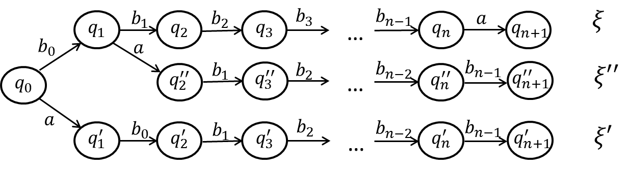
Figure 2: Potential executions $\xi,\xi^{\prime}$, and $\xi^{\prime\prime}$.

It suffices to prove that $|\xi.\mathop{\mathsf{lstate}}.X-\xi^{\prime}.\mathop{\mathsf{lstate}}.X|=|q_{n+1}.X-q_{n+1}^{\prime}.X|\leq\gamma_{n-1}(\varepsilon)$. We first construct a potential execution $\xi^{\prime\prime}=\xi_{q_{0},b_{0}ab_{1}\dots b_{n-1}}$ by swapping the first two actions of $\xi^{\prime}$. Then, $\xi^{\prime\prime}$ is of the form: $\xi^{\prime\prime}=q_{0},b_{0},q_{1},a,q_{2}^{\prime\prime},b_{1},...,b_{n-1},q_{n+1}^{\prime\prime}.$ The potential executions $\xi,\xi^{\prime}$ and $\xi^{\prime\prime}$ are shown in Figure 2. We first compare the potential executions $\xi$ and $\xi^{\prime\prime}$. Notice that, $\xi$ and $\xi^{\prime\prime}$ share a common prefix $q_{0},b_{0},q_{1}$. Starting from $q_{1}$, the action sequence of $\xi^{\prime\prime}$ is derived from $\mathit{trace}(\xi)$ by inserting action $a$ in front of the action sequence $\tau^{\prime}=b_{1}b_{2}\dots b_{n-1}$.

Since $\tau^{\prime}\stackrel{{\scriptstyle\varepsilon}}{{\sim}}a$, applying the induction hypothesis on the length $n-1$ action sequence $\tau^{\prime}$, we get $|q_{n+1}.X-q_{n+1}^{\prime\prime}.X|\leq\gamma_{n-2}(\varepsilon).$ Then, we compare the potential executions $\xi^{\prime}$ and $\xi^{\prime\prime}$. Since $b_{0}\stackrel{{\scriptstyle\varepsilon}}{{\sim}}a$, by applying the property of Definition 3 to the first two actions of $\xi^{\prime}$ and $\xi^{\prime\prime}$, we have $|q_{2}^{\prime}.X-q_{2}^{\prime\prime}.X|\leq\varepsilon$. We note that $\xi^{\prime}$ and $\xi^{\prime\prime}$ have the same suffix of action sequence from $q_{2}^{\prime}$ and $q_{2}^{\prime\prime}$. Using Proposition 1 from states $q_{2}^{\prime}$ and $q_{2}^{\prime\prime}$, we have

$$|q_{n+1}^{\prime}.X-q_{n+1}^{\prime\prime}.X|\leq\beta_{b_{1}}\beta_{b_{2}}\dots\beta_{b_{n-1}}(|q_{2}^{\prime}.X-q_{2}^{\prime\prime}.X|)\leq\beta^{n-1}(\varepsilon).$$ (3)

Combining the bound on $|q_{2}^{\prime}.X-q_{2}^{\prime\prime}.X|$ and (3) with triangular inequality, we have $|q_{n+1}.X-q_{n+1}^{\prime}.X|\leq|q_{n+1}.X-q_{n+1}^{\prime\prime}.X|+|q_{n+1}^{\prime}.X-q_{n+1}^{\prime\prime}.X|\leq\gamma_{n-2}(\varepsilon)+\beta^{n-1}(\varepsilon)=\gamma_{n-1}(\varepsilon).$ ∎

4.3 $(\delta,\varepsilon)$-trace equivalent discrepancy for traces

Lemma 1 gives a way to compute $(0,\varepsilon)$-$\mathit{ted}$. Now, we generalize this to compute $(\delta,\varepsilon)$-$\mathit{ted}$, for ($\delta,\varepsilon$)-related potential executions, with any $\delta\geq 0$. The following lemma gives an inductive way of constructing $\mathit{ted}$ as an action $a$ is appended to a trace $\tau$.

Lemma 2

For any potential execution $\xi=\xi_{q_{0},\tau}$ and constants $\delta,\varepsilon\geq 0$, if $r$ is a $(\delta,\varepsilon)$-$\mathit{ted}$ for $\xi$, and the action $a\in A$ satisfies $\tau\stackrel{{\scriptstyle\varepsilon}}{{\sim}}a$, then $r^{\prime}=\beta_{a}(r)+\gamma_{len(\tau)-1}(\varepsilon)$ is a $(\delta,\varepsilon)$-$\mathit{ted}$ for $\xi_{q_{0},\tau a}$.

Proof

Fix any $\xi^{\prime}$ that is $(\delta,\varepsilon)$-related to $\xi$ and with initial state $q_{0}^{\prime}\in{\cal B}_{\delta}(q_{0})$. It follows from Proposition 4 that $\xi^{\prime}.\mathop{\mathsf{lstate}}.L=\xi.\mathop{\mathsf{lstate}}.L$. It suffices to prove that $|\xi^{\prime}.\mathop{\mathsf{lstate}}.X-\xi.\mathop{\mathsf{lstate}}.X|\leq r^{\prime}$.

Since $\mathit{trace}(\xi^{\prime})\stackrel{{\scriptstyle\varepsilon}}{{\equiv}}\tau a$, $\mathit{trace}(\xi^{\prime})$ is in a form $\phi a\eta$ with some $\phi\eta\stackrel{{\scriptstyle\varepsilon}}{{\equiv}}\tau$. We construct a potential execution $\xi^{\prime\prime}=\xi_{q_{0}^{\prime},\phi\eta a}$. The three potential executions are illustrated in Figure 3 below.

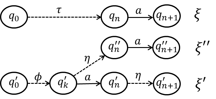
Figure 3: Execution $\xi$, its $\varepsilon$-equivalent execution $\xi^{\prime}$, and execution $\xi^{\prime\prime}$ that is constructed by swapping action $a$ to the back in $\xi^{\prime}$.

We note that $r$ is a $\mathit{ted}$ for the the prefix ($q_{0},\tau,q_{n}$) of $\xi$ and $\delta,\varepsilon$. Since $\phi\eta\stackrel{{\scriptstyle\varepsilon}}{{\equiv}}\tau$ and $q_{0}^{\prime}\in{\cal B}_{\delta}(q_{0})$, it follows from Definition 6 that $|q_{n}.X-q_{n}^{\prime\prime}.X|\leq r$. Hence

$$|\xi.\mathop{\mathsf{lstate}}.X-\xi^{\prime\prime}.\mathop{\mathsf{lstate}}.X|\leq\beta_{a}(|q_{n}.X-q_{n}^{\prime\prime}.X|)\leq\beta_{a}(r).$$ (4)

On the other hand, we observe that the traces of $\xi^{\prime}$ and $\xi^{\prime\prime}$ differ only in the position of action $a$. Application of Lemma 1 on $\xi^{\prime}$ and $\xi^{\prime\prime}$ yields

$$|\xi^{\prime}.\mathop{\mathsf{lstate}}.X-\xi^{\prime\prime}.\mathop{\mathsf{lstate}}.X|\leq\gamma_{len(\eta)-1}(\varepsilon)\leq\gamma_{len(\tau)-1}(\varepsilon).$$ (5)

Combining (4) and (5) with triangular inequality, we have

$$|\xi.\mathop{\mathsf{lstate}}.X-\xi^{\prime}.\mathop{\mathsf{lstate}}.X|\leq\beta_{a}(r)+\gamma_{len(\tau)-1}(\varepsilon).$$

∎

5 Reachability with approximate partial order reduction

We will present our main algorithm (Algorithm 2) for reachability analysis with approximate partial order reduction in this section. The core idea is to over-approximate ${\sf Reach}(B_{\delta}(q_{0}),T)$ by (a) computing the actual execution $\xi_{q_{0},\tau}$ and (b) expanding this $\xi_{q_{0},\tau}$ by a $(\delta,\varepsilon)$-$\mathit{ted}$ to cover all the states reachable from any other $(\delta_{0},\varepsilon)$-related potential execution. Combining such over-approximations from a cover of $\Theta$, we get over-approximations of ${\sf Reach}(\Theta,T)$, and therefore, Algorithm 2 can be used to soundly check for bounded safety or invariance. The over-approximations can be made arbitrarily precise by shrinking $\delta_{0}$ and $\varepsilon$ (Theorem 5.2). Of course, at $\varepsilon=0$ only traces that are exactly equivalent to $\tau$ will be covered, and nothing else. Algorithm 2 avoids computing $(\delta_{0},\varepsilon)$-related executions, and therefore, gains (possibly exponential) speedup.

The key subroutine in Algorithm 2 is $\mathit{CompTed}$ which computes the $\mathit{ted}$ by adding one more action to the traces. It turns out that, the $\mathit{ted}$ is independent of $q_{0}$, but only depends on the sequence of actions in $\tau$. $\mathit{CompTed}$ is used to compute $\delta_{t}$ from $\delta_{t-1}$, such that, $\delta_{t}$ is the $\mathit{ted}$ for the length $t$ prefix of $\xi$. Let action $a$ be the $t^{th}$ action and $\xi=\xi_{q_{0},\tau a}$. If $a$ is $\varepsilon$-independent to $\tau$, then the $\mathit{ted}$ $\delta_{t}$ can be computed from $\delta_{t-1}$ just using Lemma 2. For the case where $a$ is not $\varepsilon$-independent to the whole sequence $\tau$, we would still want to compute a set of executions that $\xi_{q_{0},\tau a}$ can cover. We observe that, with appropriate computation of $\mathit{ted}$, $\xi_{q_{0},\tau a}$ can cover all executions of the form $\xi_{q_{0},\phi a\eta}$, where $\phi a\eta$ is $\varepsilon$-equivalent to $\tau a$ and $a\notin\eta$. In what follows, we introduce this notion of earliest equivalent position of $a$ in $\tau$ (Definition 7), which is the basis for the $\mathit{CompTed}$ subroutine, which in turn is then used in the main reachability Algorithm 2.

5.1 Earliest equivalent position of an action in a trace

For any trace $\tau\in A^{*}$ and action $a\in\tau$, we define $\mathit{lastPos}(\tau,a)$ as the largest index $k$ such that $\tau(k)=a$. The earliest equivalent position, $\mathit{eep}(\tau,a,\varepsilon)$ is the minimum of $\mathit{lastPos}(\tau^{\prime},a)$ in any $\tau^{\prime}$ that is $\varepsilon$-equivalent to $\tau a$.

Definition 7

For any trace $\tau\in A^{*}$, $a\in A$, and $\varepsilon>0$, the earliest equivalent position of $a$ on $\tau$ is $\mathit{eep}(\tau,a,\varepsilon)\mathrel{\stackrel{{\scriptstyle\scriptscriptstyle\Delta}}{{=}}}\min_{\tau^{\prime}\stackrel{{\scriptstyle\varepsilon}}{{\equiv}}\tau a}\mathit{lastPos}(\tau^{\prime},a).$

For any trace $\tau a$, its $\varepsilon$-equivalent traces can be derived by swapping consecutive $\varepsilon$-independent action pairs. Hence, the eep of $a$ is the leftmost position it can be swapped to, starting from the end. Any equivalent trace of $\tau a$ is of the form $\phi a\eta$ where $\phi$ and $\eta$ are the prefix and suffix of the last occurrence of action $a$. Hence, equivalently: $\mathit{eep}(\tau,a,\epsilon)=\min_{\phi a\eta\stackrel{{\scriptstyle\varepsilon}}{{\equiv}}\tau a,\ a\notin\eta}len(\phi).$ In Appendix 0.A.1 we give a simple $O(len(\tau)^{2})$ algorithm for computing $\mathit{eep}()$. If the $\varepsilon$-independence relation is symmetric, then it $\mathit{eep}$ can be computed in $O(len(\tau))$ time.

Example 5

In Example 3, we showed that $a_{0}\stackrel{{\scriptstyle\varepsilon}}{{\sim}}a_{1}$ and $a_{0}\stackrel{{\scriptstyle\varepsilon}}{{\sim}}a_{2}$ with $\varepsilon=0.1$; $a_{\bot}$ is not $\varepsilon$-independent to any actions. What is $\mathit{eep}(a_{\bot}a_{0}a_{1},a_{2},\varepsilon)$? We can swap $a_{2}$ ahead following the sequence $\tau a_{2}=a_{\bot}a_{0}a_{1}a_{2}\stackrel{{\scriptstyle\varepsilon}}{{\equiv}}a_{\bot}a_{1}a_{0}a_{2}\stackrel{{\scriptstyle\varepsilon}}{{\equiv}}a_{\bot}a_{1}a_{2}a_{0}$. As $a_{\bot}$ and $a_{1}$ are not independent of $a_{2}$, it cannot occur earlier. $\mathit{eep}(a_{\bot}a_{0}a_{1},a_{2},\varepsilon)=2$.

5.2 Reachability using $(\delta,\varepsilon)$-trace equivalent discrepancy

$\mathit{CompTed}$ (Algorithm 1) takes inputs of trace $\tau$, a new action to be added $a$, a parameter $r\geq 0$ such that $r$ is a $(\delta_{0},\varepsilon)$-$\mathit{ted}$ for the potential execution $\xi_{q_{0},\tau}$ for some initial state $q_{0}$, initial set radius $\delta_{0}$, approximation parameter $\varepsilon\geq 0$, and a set of discrepancy functions $\{\beta_{a}\}_{a\in A}$. It returns a $(\delta_{0},\varepsilon)$-$\mathit{ted}$ $r^{\prime}$ for the potential execution $\xi_{q_{0},\tau a}$.

Algorithm 1 $\mathit{CompTed}(\tau,a,r,\varepsilon,\{\beta_{a}\}_{a\in A})$

1:$\beta\leftarrow\max_{b\in\tau a}\{\beta_{b}\}$; $k\leftarrow\mathit{\mathit{eep}(\tau,a,\epsilon)}$; $t\leftarrow len(\tau)$;

2:if $k=t$ then $r^{\prime}\leftarrow\beta_{a}(r)$ else $r^{\prime}\leftarrow\beta_{a}(r)+\gamma_{t-k-1}(\varepsilon)$

3:return $r^{\prime}$;

Lemma 3

For some initial state $q_{0}$ and initial set size $\delta_{0}$, if $r$ is a $(\delta_{0},\varepsilon)$-$\mathit{ted}$ for $\xi_{q_{0},\tau}$ then value returned by $\mathit{CompTed}()$ is a $(\delta_{0},\varepsilon)$-$\mathit{ted}$ for $\xi_{q_{0},\tau a}$.

Proof

Let us fix some initial state $q_{0}$ and initial set size $\delta_{0}$.

Let $\xi_{t}=\xi_{q_{0},\tau}$ be the potential execution starting from $q_{0}$ by taking the trace $\tau$, and $\xi_{t+1}=\xi_{q_{0},\tau a}$. Fix any $\xi^{\prime}$ that is ($\delta_{0},\varepsilon$)-related to $\xi_{t+1}$. From Proposition 4, $\xi^{\prime}.\mathop{\mathsf{lstate}}.L=\xi_{t+1}.\mathop{\mathsf{lstate}}.L$. It suffice to prove that $|\xi^{\prime}.\mathop{\mathsf{lstate}}.X-\xi_{t+1}.\mathop{\mathsf{lstate}}.X|\leq r^{\prime}$.

Figure 4: Potential executions $\xi_{t+1}$, $\xi^{\prime}$,$\xi^{\prime\prime}$

Since $\mathit{trace}(\xi^{\prime})\stackrel{{\scriptstyle\varepsilon}}{{\equiv}}\tau a$, action $a$ is in the sequence $\mathit{trace}(\xi^{\prime})$. Partitioning $\mathit{trace}(\xi^{\prime})$ on the last occurrence of $a$, we get $\mathit{trace}(\xi^{\prime})=\phi a\eta$ for some $\phi,\eta\in A^{*}$ with $a\not\in\eta$. Since $k$ is the $eep$, from Definition 7, the position of the last occurrence of $a$ on $\mathit{trace}(\xi^{\prime})$ is at least $k$. Hence we have $len(\phi)\geq k$ and $len(\eta)=t-len(\phi)\leq t-k$. We construct another potential execution $\xi^{\prime\prime}=\xi_{q^{\prime}_{0},\phi\eta a}$ with the same initial state as $\xi^{\prime}$. The executions $\xi_{t+1},\xi^{\prime}$ and $\xi^{\prime\prime}$ are illustrated in Figure 4.

$q_{t}$ is the last state of the execution $\xi_{t}$. From the assumption, ${\cal B}_{r}(q_{t})$ is an over-approximation of the reachset at step $t$. We note that the length $t$ prefix $\xi^{\prime\prime}$ is ($\delta_{0},\varepsilon$)-related to $\xi_{t}$. Therefore, $|q_{t}.X-q_{t}^{\prime\prime}.X|\leq r$. Using the discrepancy function of action $a$, we have

$$|q_{t+1}.X-q_{t+1}^{\prime\prime}.X|\leq\beta_{a}(|q_{t}.X-q_{t}^{\prime\prime}.X|)\leq\beta_{a}(r).$$ (6)

We will quantify the distance between $\xi^{\prime}$ and $\xi^{\prime\prime}$. There are two cases:
(i) If $k=t$ then, $len(\eta)\leq t-k=0$, that is, $\eta$ is an empty string. Hence, $\xi^{\prime}$ and $\xi^{\prime\prime}$ are indeed identical and $q^{\prime}_{t+1}=q^{\prime\prime}_{t+1}$. Thus from (6), $|q_{t+1}.X-q^{\prime}_{t+1}.X|=|q_{t+1}.X-q_{t+1}^{\prime\prime}.X|\leq\beta_{a}(r),$ and the lemma holds. (ii) Otherwise $k<t$ and from Lemma 1, we can bound the distance between $\xi^{\prime}$ and $\xi^{\prime\prime}$ as $|q_{t+1}^{\prime}.X-q_{t+1}^{\prime\prime}.X|\leq\gamma_{len(\eta)-1}(\varepsilon)\leq\gamma_{t-k-1}(\varepsilon).$ Combining with (6), we get $|q_{t+1}.X-q^{\prime}_{t+1}.X|\leq|q_{t+1}.X-q^{\prime\prime}_{t+1}.X|+|q^{\prime}_{t+1}.X-q^{\prime\prime}_{t+1}.X|\leq\beta_{a}(r)+\gamma_{t-k-1}(\varepsilon).$ ∎

Next, we present the main reachability algorithm which uses $\mathit{CompTed}$. Algorithm 2 takes inputs of an initial set $\Theta$, time horizon $T$, two parameters $\delta_{0},\varepsilon\geq 0$, and a set of discrepancy functions $\{\beta_{a}\}_{a\in A}$. It returns the over-approximation of the reach set for each time step.

The algorithm first computes a $\delta_{0}$-cover $Q_{0}$ of the initial set $\Theta$ such that $\Theta\subseteq\cup_{q_{0}\in Q_{0}}{\cal B}_{\delta}(q_{0})$ (Line 2). The for-loop from Line 3 to Line 14 will compute the over-approximation of the reachset from each initial cover ${\sf Reach}({\cal B}_{\delta_{0}}(q_{0}),t)$. The over-approximation from each cover is represented as a collection $\langle R_{0},\dots,R_{T}\rangle$, where each $R_{t}$ is a set of tuples $\langle\tau_{t},q_{t},\delta_{t}\rangle$ such that (i) the traces $R_{t}\mathrel{\lceil}1$ and their $\varepsilon$-equivalent traces contain the traces of all valid executions of length $t$, (ii) the traces in $R_{t}\mathrel{\lceil}1$ are mutually non-$\varepsilon$-equivalent, (iii) for each tuple $\delta_{t}$ is the $(\delta_{0},\varepsilon)$-$\mathit{ted}$ for $\xi_{q_{0},\tau_{t}}$,

For each initial cover ${\cal B}_{\delta_{0}}(q_{0})$, $R_{0}$ is initialized as the tuple of empty string, the initial state $q_{0}$ and size $\delta_{0}$ (Line 4). Then the reachset over-approximation is computed recursively for each time step by checking for the maximum set of enabled actions $EA$ for the set of states ${\cal B}_{\delta_{t}}(q_{t})$ (Line 8), and try to attach each enabled action $a\in EA$ to $\tau_{t}$ unless $\tau_{t}a$ is $\varepsilon$-equivalent to some length $t+1$ trace that is already in $R_{t+1}\mathrel{\lceil}1$. This is where the major reduction happens using approximate partial order reduction. If not, the $(\delta_{0},\varepsilon)$-$\mathit{ted}$ for $\xi_{q_{0},\tau_{t}a}$ will be computed using $\mathit{CompTed}$, and new tuple $\langle\tau_{t}a,q_{t+1},\delta_{t+1}\rangle$ will be added to $R_{t+1}$ (Line 13).

If there are $k$ actions in total and they are mutually $\varepsilon$-independent, then as long as the numbers of each action in $\tau_{t}$ and $\tau^{\prime}_{t}$ are the same, $\tau_{t}\stackrel{{\scriptstyle\varepsilon}}{{\equiv}}\tau^{\prime}_{t}$. Therefore, in this case, $R_{t}$ contains at most $\binom{t+k-1}{k-1}$ tuples. Furthermore, for any length $t$ trace $\tau_{t}$, if all actions in $\tau_{t}$ are mutually $\varepsilon$-independent, the algorithm can reduce the number of executions explored by $O(t!)$. Essentially, each $\tau_{t}\in R_{t}\mathrel{\lceil}1$ is a representative trace for the length $t$ $\varepsilon$-equivalence class.

Algorithm 2 Reachability algorithm to over-approximate ${\sf Reach}(\Theta,T)$

1:Input: $\Theta,T,\varepsilon,\delta_{0},\{\beta_{a}\}$;

2:$Q_{0}\leftarrow\delta_{0}$-$cover(\Theta)$; ${\cal R}\leftarrow\emptyset$

3:for $q_{0}\in Q_{0}$ do

4:     $R_{0}\leftarrow\{\langle^{\prime\prime},q_{0},\delta_{0}\rangle\}$;

5:     for $t=[T]$ do

6:         $R_{T}\leftarrow\emptyset$;

7:         for  each $\langle\tau_{t},q_{t},\delta_{t}\rangle\in R_{t}$ do

8:              $EA\leftarrow enabledactions({\cal B}_{\delta_{t}}(q_{t}))$;

9:              for $a\in EA$ do

10:                  if $\forall\tau_{t+1}\in R_{t+1}\mathrel{\lceil}1,\neg\left(\tau_{t}a\stackrel{{\scriptstyle\varepsilon}}{{\equiv}}\tau_{t+1}\right)$ then;

11:                       $q_{t+1}\leftarrow a(q_{t})$

12:                       $\delta_{t+1}\leftarrow\mathit{CompTed}(\tau_{t},a,\delta_{t},\varepsilon,\{\beta_{a}\}_{a\in A})$

13:                       $R_{t+1}\leftarrow R_{t+1}\cup\langle\tau_{t}a,q_{t+1},\delta_{t+1}\rangle$                                                

14:     ${\cal R}\leftarrow{\cal R}\cup\langle R_{0},\dots,R_{T}\rangle$

15:return ${\cal R}$;

Theorem 5.1 shows that Algorithm 5.1 indeed computes an over-approximation for the reachsets, and Theorem 5.2 states that the over-approximation can be made arbitrarily precise by reducing the size of $\delta_{0},\varepsilon$.

Theorem 5.1 (Soundness)

Set ${\cal R}$ returned by Algorithm 2, satisfies $\forall t=0,\dots,T,$

$${\sf Reach}(\Theta,t)\subseteq\bigcup_{R_{t}\in{\cal R}\mathrel{\lceil}t}\bigcup_{\langle\tau,q,\delta\rangle\in R_{t}}{\cal B}_{\delta}(q).$$ (7)

Proof

Since $\cup_{q_{0}\in Q_{0}}{\cal B}_{\delta}(q_{0})\supseteq\Theta$, it suffices to show that at each time step $t=0,\dots,T$, the $R_{t}$ computed in the for-loop from Line 4 to Line 13 satisfy ${\sf Reach}({\cal B}_{\delta_{0}}(q_{0}),t)\subseteq\cup_{\langle\tau,q,\delta\rangle\in R_{t}}{\cal B}_{\delta}(q)$. Fix any $q_{0}\in Q_{0}$, we will prove by induction.

Base case: initially before any action happens, the only valid trace is the empty string ^′′ and the initial set is indeed ${\cal B}_{\delta_{0}}(q_{0})$.

Induction step: assume that at time step $t<T$, the union of all the traces $R_{t}\mathrel{\lceil}1$ and their $\varepsilon$-equivalent traces contain the traces of all length $t$ valid executions, and for each tuple $\langle\tau_{t},q_{t},\delta_{t}\rangle\in R_{t}$, $\delta_{t}$ is a $(\delta_{0},\varepsilon)$-$\mathit{ted}$ for $\xi_{q_{0},\tau_{t}}$. That is, ${\cal B}_{\delta_{t}}(q_{t})$ contains the final states of all ($\delta_{0},\varepsilon$)-related executions to $\xi_{q_{0},\tau_{t}}$. This is sufficient for showing that ${\sf Reach}({\cal B}_{\delta_{0}}(q_{0}),t)\subseteq\cup_{\langle\tau,q,\delta\rangle\in R_{t}}{\cal B}_{\delta}(q)$.

Since for each tuple contained in $R_{t}$, we will consider the maximum possible set of actions enabled at Line 8 and attempts to compute the $(\delta_{0},\varepsilon)$-$\mathit{ted}$ for $\xi_{q_{0},\tau_{t}a}$. If $\tau_{t}a$ is not $\varepsilon$-equivalent to any of the length $t+1$ traces that has already been added to $R_{t+1}$, then Lemma 3 guarantees that the $q_{t+1}$ and $\delta_{t+1}$ computed at Line 11 and 12 satisfy that $\delta_{t+1}$ is the $(\delta_{0},\varepsilon)$-$\mathit{ted}$ for $\xi_{q_{0},\tau_{t}a}$. Otherwise, $\tau_{t}a$ is $\varepsilon$-equivalent to some trace $\tau_{t+1}$ that has already been added to $R_{t+1}$, then for any initial state $q_{0}^{\prime}$ that is $\delta_{0}$-close to $q_{0}$, $\xi_{q_{0}^{\prime},\tau_{t}a}$ and $\xi_{q_{0},\tau_{t+1}}$ are $(\delta_{0},\varepsilon)$-related and the final state of $\xi_{q^{\prime}_{0},\tau_{t}a}$ is already contained in ${\cal B}_{\delta_{t+1}}(q_{t+1})$. Therefore, the union of all the traces $R_{t+1}\mathrel{\lceil}1$ and their $\varepsilon$-equivalent traces contain the traces of all length $t+1$ valid executions, and for each tuple $\langle\tau_{t+1},q_{t+1},\delta_{t+1}\rangle\in R_{t+1}$, $\delta_{t+1}$ is a $(\delta_{0},\varepsilon)$-$\mathit{ted}$ for $\xi_{q_{0},\tau_{t+1}}$, which means ${{\sf Reach}({\cal B}_{\delta_{0}}(q_{0}),t+1)}\subseteq\cup_{\langle\tau,q,\delta\rangle\in R_{t+1}}{\cal B}_{\delta}(q)$. So the theorem holds. ∎

Theorem 5.2 (Precision)

For any $r>0$, there exist $\delta_{0},\varepsilon>0$ such that, the reachset over-approximation ${\cal R}$ computed by Algorithm 2 satisfies $\forall t=0,\dots,T,$

$$\bigcup_{R_{t}\in{\cal R}\mathrel{\lceil}t}\bigcup_{\langle\tau,q,\delta\rangle\in R_{t}}{\cal B}_{\delta}(q)\subseteq{\cal B}_{r}({\sf Reach}(\Theta,t)).$$ (8)

Proof

From Proposition 2, for any $n$, $\gamma_{n}(\varepsilon)\rightarrow 0$ as $\varepsilon\rightarrow 0$. From Definition 2, for any $\delta_{t}$ and discrepancy function $\beta$, $\beta(\delta_{t})\rightarrow 0$ as $\delta_{t}\rightarrow 0$. Therefore, when Line 12 of Algorithm 2 is executed, $\delta_{t+1}\rightarrow 0$ as $\delta_{t}\rightarrow 0$ and $\varepsilon\rightarrow 0$. Iteratively applying this observation leads that $\delta_{t}$ contained in any set $R_{t}$ converges to zero as $\delta_{0}\rightarrow 0$ and $\varepsilon\rightarrow 0$.

Fix arbitrary $r>0$. The set ${\cal R}$ is a union of approximations for each ${\sf Reach}({\cal B}_{\delta_{0}}(q_{0}),T)$. Fix any such $q_{0},\delta_{0}$, it suffices to show that $\cup_{\langle\tau,q,\delta\rangle\in R_{t}}{\cal B}_{\delta}(q)\subseteq{\cal B}_{r}({\sf Reach}(\Theta,t))$ for small enough $\delta_{0}$ and $\varepsilon$. Moreover, it suffices to show that fix any $\langle\tau_{t},q_{t},\delta_{t}\rangle\in R_{t}$, ${\cal B}_{\delta}(q_{t})\subseteq{\cal B}_{r}({\sf Reach}(\Theta,t))$ for small enough $\delta_{0}$ and $\varepsilon$.

Since each $\delta_{t}$ is a $(\delta_{0},\varepsilon)$-$\mathit{ted}$ of the execution $\xi_{q_{0},\tau_{t}}$ and $\delta_{0},\varepsilon$, there is an execution $\xi^{\prime}=\xi^{\prime}_{q^{\prime}_{0},\tau^{\prime}}$ from $q^{\prime}_{0}\in{\cal B}_{\delta}(q_{0})$ following the trace $\tau^{\prime}\stackrel{{\scriptstyle\varepsilon}}{{\equiv}}\tau_{t}$. By the definition of reachset, we have $\xi^{\prime}(t)\in{\sf Reach}(\Theta,t)$. On the other hand, $\xi^{\prime}$ is ($\delta_{0},\varepsilon$)-related to the potential execution $\xi_{q_{0},\tau_{t}}$, so $\xi^{\prime}(t)\in{\cal B}_{\delta_{t}}(q_{t})$. That is, ${\cal B}_{\delta_{t}}(q_{t})$ and the reachset ${\sf Reach}(\Theta,t)$ has intersections at the state $\xi^{\prime}(t)$.

The radius of at each time step $\delta_{t}$ can be made arbitrarily small as $\delta_{0}$ and $\varepsilon$ go to $0$. We chose small enough $\delta_{0}$ and $\varepsilon$, such that the radius of ${\cal B}_{\delta_{t}}(q_{t})$ is less than $r/2$. Therefore, ${\cal B}_{\delta_{t}}(q_{t})$ is contained in the radius $r$ ball of the reachset ${\cal B}_{r}({\sf Reach}(\Theta,t))$. ∎

Notice that as $\delta_{0}$ and $\varepsilon$ go to $0$, the Algorithm 2 actually converges to a simulation algorithm which simulates every valid execution from a single initial state.

6 Experimental evaluation of effectiveness

We discuss the results from evaluating Algorithm 2 in three case studies. Our Python implementation runs on a standard laptop (Intel Core^TM i7-7600 U CPU, 16G RAM).

Iterative consensus.

This is an instance of ${\operatorname{\mathsf{Consensus}}}$ (Example 1) with $3$ continuous variables and 3 actions $a_{0},a_{1},a_{2}$. We want to check if the continuous states converge to $[-0.4,0.4]^{3}$ in 3 rounds starting from a radius $0.5$ ball around $[2.5,0.5,-3]$. Figure 5 (Left) shows reachset over-approximation computed and projected on $x[0]$. The blue and red curves give the bounds. As the figure shows, $x[0]$ converges to $[-0.4,0.4]$ at round 3; and so do $x[1]$ and $x[2]$ (not shown). We also simulated $100$ random valid executions (yellow curves) from the initial set and validate that indeed the over-approximation is sound.

Recall, three actions can occur in any order in each round, i.e., $3!=6$ traces per round, and $6^{3}=216$ executions from a single initial state up to $3$ rounds. We showed in Example 3 that $a_{0}\stackrel{{\scriptstyle\varepsilon}}{{\sim}}a_{1}$ and $a_{0}\stackrel{{\scriptstyle\varepsilon}}{{\sim}}a_{2}$ with $\varepsilon=0.1$. Therefore, $a_{0}a_{1}a_{2}\stackrel{{\scriptstyle\varepsilon}}{{\equiv}}a_{1}a_{0}a_{2}\stackrel{{\scriptstyle\varepsilon}}{{\equiv}}a_{1}a_{2}a_{0}$ and $a_{0}a_{2}a_{1}\stackrel{{\scriptstyle\varepsilon}}{{\equiv}}a_{2}a_{0}a_{1}\stackrel{{\scriptstyle\varepsilon}}{{\equiv}}a_{2}a_{1}a_{0}$, and Algorithm 2 explored only $2$ (length $12$) executions from a set of initial states for computing the bounds. The running time for Algorithm 2 is 1 millisecond while exploring all valid executions from even only a single state took 20 milliseconds.

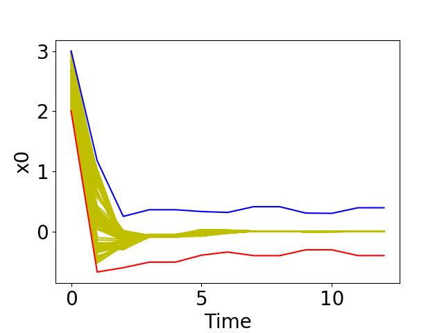
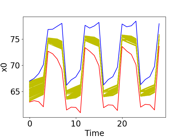
Figure 5: Reachset computations. The blue curves are the upper bound of the reachsets and the red curves are the lower bound of the reachsets. Between the blue and red curves, the yellow curves are $100$ random simulations of valid executions. Left: Linear transition system. Right: Room heating system.

Platoon.

Consider an $N$ car platoon on a single lane (see Figure 7 in Appendix 0.A.2.1 for the pseudocode and details). Each car can choose one of three actions at each time step: $a$ (accelerate), $b$ (brake), or $c$ (cruise). Car $0$ can choose any action at each time step; remaining cars try to keep safe distance with predecessor by choosing accelerate ($a$) if the distance is more than $50$, brake ($b$) if the distance is less than $30$, and cruise ($c$) otherwise.

Consider a 2-car platoon and a time horizon of $T=10$. We want to verify that the cars maintain safe separation. Reachset over-approximations projected on the position variables are shown in Figure 6, with $100$ random simulations of valid executions as a sanity check. Car 0 has lots of choices and it’s position over-approximation diverges (Figure 6). Car 1’s position depends on its initial relative distance with Car 0. It is also easy to conclude from Figure 6 that two cars maintain safe relative distance for these different initial states.

From a single initial state, in every step, Car 0 has $3$ choices, and therefore there are $3^{10}$ possible executions. Considering a range of initial positions for two cars, there are infinitely many execution, and $9^{10}$ (around 206 trillion) possible traces. With $\epsilon=0.282$, Algorithm 2 explored a maximum of $\binom{18}{8}=43758$ traces; the concrete number varies for different initial sets. The running time for Algorithm 2 is 5.1 milliseconds while exploring all valid executions from even only a single state took 2.9 seconds.

For a 4-car platoon and a time horizon of $T=10$, there are $81^{10}$ possible traces considering a range of initial positions. With $\varepsilon=0.282$, Algorithm 2 explored $7986$ traces to conclude that all cars maintain safe separation for the setting where all cars are initially separated by a distance of $40$ and has an initial set radius of $4$. The running time for Algorithm 2 is 62.3 milliseconds, while exploring all valid executions from even only a single state took 6.2 seconds.

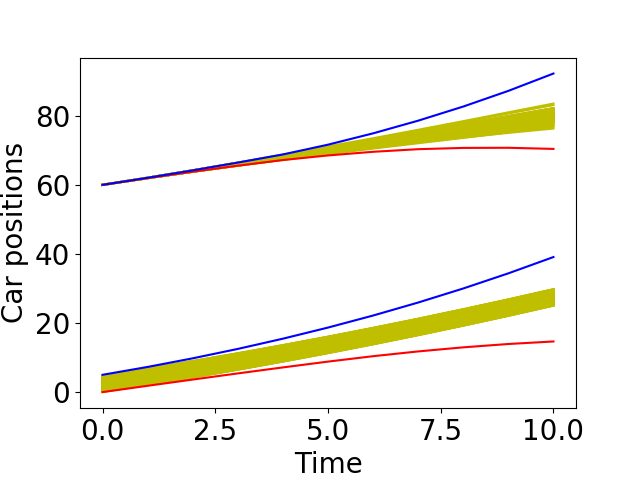
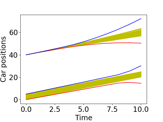
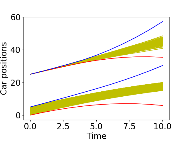
Figure 6: Position over-approximations for 2 cars. The blue curves are the upper bound of the reachsets and the red curves are the lower bound of the reachsets. Between the blue and red curves, the yellow curves are $100$ random simulations of valid executions. Car1’s initial position is in the range $[0,5]$, Car2’s initial position is $60$ (Left), $40$ (Center) and $25$ (Right).

Building heating system.

Consider a building with $N$ rooms, each with a heater (see Appendix 0.A.2.2 for pseudocode and details). For $i\in[N]$, $x[i]\in{\mathbb{R}}$ is the temperature of room $i$ and $m[i]\in\{0,1\}$ captures the off/on state of it’s heater. The controller measures the temperature of rooms periodically; based on these measurements ($y[i]$) heaters turn on or off. These decisions are made asynchronously across rooms in arbitrary order. The room temperature $x[i]$ changes linearly according to the heater input $m[i]$, the thermal capacity of the room, and the thermal coupling across adjacent rooms as given in the benchmark problem of [17]. For $i\in[N]$, actions ${\operatorname{\mathsf{on}}}_{i},{\operatorname{\mathsf{off}}}_{i}$ capture the decision making process of room $i$ on whether or not to turn on the heater. Time elapse is captured by a ${\operatorname{\mathsf{flow}}}$ action that updates the temperatures. We want to verify that the room temperatures remain in the $[60,79]$ range.

Consider a building with $N=3$ rooms. In Appendix 0.A.2.2, we provide computation details to show that for any $i,j\in[3]$ with $i\neq j$, $a\in\{{\operatorname{\mathsf{on}}}_{i},{\operatorname{\mathsf{off}}}_{i}\}$ and $b\in\{{\operatorname{\mathsf{on}}}_{j},{\operatorname{\mathsf{off}}}_{j}\}$, $a\stackrel{{\scriptstyle\varepsilon}}{{\sim}}b$ with $\varepsilon=0.6$; but, ${\operatorname{\mathsf{flow}}}$ is not independent with any other actions. Computed reachset over-approximation for 8 rounds and projected on the temperature of Room 0 is shown in Figure 5 (Right). Indeed, temperature of Room 0 is contained within the range.

For a round, where each room makes a decision once in arbitrary order, there are $3!=6$ $\varepsilon$-equivalent action sequences. Therefore, from a single initial state, there are $6^{8}$ (1.6 million) valid executions. Algorithm 2, in this case explore only one (length $32$) execution with $\varepsilon=0.6$ to approximate all executions starting from an initial set with radius $\delta=2$. The running time for Algorithm 2 is 1 millisecond while exploring all valid executions from even only a single state took 434 seconds.

7 Conclusion

We proposed a partial order reduction technique for reachability analysis of infinite state transition systems that exploits approximate independence and bounded sensitivity of actions to reduce the number of executions explored. This relies on a novel notion of $\varepsilon$-independence that generalizes the traditional notion of independence by allowing approximate commutation of actions. With this $\varepsilon$-independence relation, we have developed an algorithm for soundly over-approximating reachsets of all executions using only $\varepsilon$-equivalent traces. The over-approximation can also be made arbitrarily precise by reducing the size of $\delta,\varepsilon$. In experimental evaluation with three case studies we observe that it can reduce the number of executions explored exponentially compared to explicit computation of all executions.

The results suggest several future research directions. In Definition 3, $\varepsilon$-independent actions are required to be approximately commutative globally. For reachability analysis, this definition could be relaxed to actions that approximately commute locally over parts of the state space. An orthogonal direction is to apply this reduction technique to verify temporal logic properties and extend it to hybrid models.

Appendix 0.A Appendix

0.A.1 Algorithm to compute the earliest equivalent point

In the following algorithm, we find the earliest equivalent point $eep$ of action $a$ on an action sequence $\tau$. For any trace $\tau$ and action $a$, $eep(\tau,a,\varepsilon)$ constructs a trace $\phi\in A^{*}$. Initially $\phi$ is set to be the empty sequence. Iteratively, from the end of $\tau$, we add action $\tau(t)$ to $\phi$ if it is not independent to the entire trace $\phi a$. We will prove that, length of $\phi$ gives the $eep$ of action $a$ on trace $\tau$. The time complexity of the algorithm is at most $O(n^{2})$, where $n$ is the length of trace $\tau$.

Algorithm 3 eep($\tau,a,\varepsilon$)

1:$\phi\leftarrow\langle\rangle$;

2:$T\leftarrow len(\tau)$;

3:for $t=T-1:0$ do

4:     if $\exists b\in\phi a,\tau(t)\not\stackrel{{\scriptstyle\varepsilon}}{{\sim}}b$  then

5:         $\phi\leftarrow\tau(t)\phi$;      

6:return $len(\phi)$;

Lemma 4

For any action $a\in A$ and trace $\tau\in A^{*}$, the function $eep(\tau,a,\varepsilon)$ computes the $eep$ of $a$ on $\tau$.

Proof

For a trace $\tau$ and an action $a$, algorithm $eep(\tau,a,\varepsilon)$ constructs a trace $\phi$ and returns its length. To prove that $len(\phi)$ gives the $eep$ $k$ of $a$ on $\tau$, we show both $len(\phi)\geq k$ and $len(\phi)\leq k$.

$len(\phi)\geq k$: It suffice to prove the statement by constructing a trace $\eta$ such that $\phi a\eta\stackrel{{\scriptstyle\varepsilon}}{{\equiv}}\tau a$ and $a\notin\eta$. Let $\eta=\tau\backslash\phi$ be the remaining subsequence of $\tau$ after removing the actions in $\phi$. We note that the ordering of actions in $\eta$ is the same as that in $\tau$. For each action $c\in\eta$, line 5 is not executed. Hence, for all actions $b\in\phi a$ which is originally to the right of $c$, we have $b\stackrel{{\scriptstyle\varepsilon}}{{\sim}}c$. Therefore, action $c$ can be swapped repeatedly to the right of action $a$. Repeat this process for all actions in $\eta$, we derive trace $\phi a\eta$ from the original trace $\tau a$. Therefore $\phi a\eta\stackrel{{\scriptstyle\varepsilon}}{{\equiv}}\tau a$. In addition, we note that from Definition 3, an $\varepsilon$-independent action pair consists of two distinctive actions, which implies $a\not\stackrel{{\scriptstyle\varepsilon}}{{\sim}}a$. Hence, for each occurrence $a\in\tau$, line 5 is not executed, that is, $a\notin\eta$. Therefore, the statement holds.

$len(\phi)\leq k$: First, we convert any trace $\tau a$ to a trace consists of only distinctive actions. If otherwise some action $b\in\tau a$ occurs more than once, we replace the occurrences as distinctive pseudo-actions $b_{0},b_{1},\dots$, such that each $b_{i}$ inherit the same independence relation from $b$ and any pair of these pseudo-actions is not independent. In this way, we map an arbitrary trace $\tau a$ to a trace consists of only distinctive actions. It can be checked that this mapping is bijective. Without loss of generality, we assume that the actions in $\tau a$ are distinctive.
We prove $len(\phi)\leq k$ by contradiction. Suppose $len(\phi)>k$, then there exist traces $\phi^{\prime},\eta^{\prime}$ such that (i) $a\notin\eta^{\prime}$, (ii) $\phi^{\prime}a\eta^{\prime}\stackrel{{\scriptstyle\varepsilon}}{{\equiv}}\tau a$, and (iii) $len(\phi^{\prime})<len(\phi)$. From (iii), there exists an action $c\in\phi\backslash\phi^{\prime}$. If there are multiple choices of such actions, we choose the rightmost action $c$ in $\phi$. From line 4 and 5, action $c$ is in $\phi$ iff there exists another action $b\in\phi$ to the right of $c$ such that $c\not\stackrel{{\scriptstyle\varepsilon}}{{\sim}}b$. Since we choose action $c$ as the rightmost action in $\phi$ that is not in $\phi^{\prime}$, we have $b\in\phi^{\prime}$. Originally in trace $\tau a$, action $b$ is to the right of action $c$. As actions $b$ and $c$ are not $\varepsilon$-independent, in any equivalent trace $\phi^{\prime}a\eta^{\prime}\stackrel{{\scriptstyle\varepsilon}}{{\equiv}}\tau a$, the relative position of them should not be changed. Hence in trace $\phi^{\prime}a\eta^{\prime}$, action $b$ is also to the right of action $c$. However, since $b\in\phi^{\prime}$ and $c\notin\phi^{\prime}$, we have action $c$ is to the right of action $b$ in trace $\phi^{\prime}a\eta^{\prime}$. We derive a contradiction. Therefore, if the actions in $\tau a$ are distinctive, $len(\phi)\leq k$.

0.A.2 Complete description of the examples

0.A.2.1 Platoon.

Consider an $N$ car platoon on a single lane road (see Figure 7). Each car can choose one of three actions at each time step: $a$ (accelerate), $b$ (brake), or $c$ (cruise). Car $0$ can choose any action at each time step; remaining cars try to keep safe distance with predecessor by choosing accelerate ($a$) if the distance is more than $50$, brake ($b$) if the distance is less than $30$, and cruise ($c$) otherwise. For each $i\in[N]$, $x[2i]$ is the position, $x[2i+1]$ is the velocity, and $m[i]$ is the chosen action, of the $i^{th}$ car. At each step, $m[i]$ is updated using relative positions according to the rule described above, and then $x$ is updated according to the actions. For concreteness, the linear state transition equation for a 2-car platoon is shown below:

  ⬇ 1automaton ${\operatorname{\mathsf{CarPlatoon}}}(N:{\operatorname{\texttt{Nat}}})$ variables 3 $x:{\operatorname{\texttt{Real}}}^{2N}$ ; $m:\{c,a,b\}^{N}$; 5 initially 7 $\mbox{for each }i\in[N]$ $m[i]:=$ choose $\{c,a,b\}$; ⬇ transitions 11 ${\operatorname{\mathsf{move}}}$ pre true 13 eff $m[0]:=$ choose $\{c,a,b\}$; $\mbox{for each }i\in[N]\setminus 0$ 15 $m[i]:=\left\{\begin{array}[]{ll}a&\mbox{ if }x[2(i-1)]-x[2i]>50\\ b&\mbox{ if }x[2(i-1)]-x[2i]<30\\ c&\mbox{ else }\\ \end{array}\right.$; $x:=Ax+b_{m}$;  

Figure 7: Labeled transition system model of cars keeping a platoon.

$$\small x\leftarrow\begin{bmatrix}1&\Delta t&0&0\\ 0&1&0&0\\ 0&0&1&\Delta t\\ 0&0&0&1\\ \end{bmatrix}x+\begin{bmatrix}\frac{acc_{0}(\Delta t)^{2}}{2}\\ acc_{0}\Delta t\\ \frac{acc_{1}(\Delta t)^{2}}{2}\\ acc_{1}\Delta t\\ \end{bmatrix}=Ax+b_{m},$$ (9)

where $acc_{i}>0$ if car $i$ accelerates; $acc_{i}<0$ if it brakes; and $acc_{i}=0$ if it cruises. For any value of $m$, the discrepancy function for the corresponding actions are the same: For any $q,q^{\prime}$ with $q.L=q^{\prime}.L$, $\beta_{a}(|q.x-q^{\prime}.x|)=|A||q.x-q^{\prime}.x|$. For any $i,j\in[9]$ with $i\neq j$, we notice that $|a_{i}a_{j}(q).x-a_{j}a_{i}(q).x|=|Ab_{m_{i}}-Ab_{m_{j}}+b_{m_{j}}-b_{m_{i}}|$ which is a constant number and can be used as $\varepsilon$. If we choose $\Delta t=0.1$, then the discrepancy function could be $\beta_{a}(|q.x-q^{\prime}.x|_{2})=1.06|q.x-q^{\prime}.x|_{2}$. Furthermore, if $acc_{i}$ can choose from $\{-10,0\}$, or from $\{10,0\}$, then the corresponding actions are $\varepsilon$-independent with $\epsilon=0.141$, and if $acc_{i}$ can choose from $\{-10,0,10\}$, then the corresponding actions are $\varepsilon$-independent with $\epsilon=0.282$.

0.A.2.2 Room heating problem

We present a building heating system in Fig. 8. The building has $N$ rooms each with a heater. For $i\in[N]$, $x[i]\in{\mathbb{R}}$ is the temperature of room $i$ and $m[i]\in\{0,1\}$ captures the off/on state of the heater in the room. The building measures the temperature of rooms periodically every $T$ seconds and save the measurements to $y[i]$. Based on the measurement $y[i]$, each room takes action $a_{i}$ to decide whether to turn on or turn off its heater. The boolean variable $d[i]$ indicates whether room $i$ has made a decision. These decisions are made asynchronously among the rooms with a small delay $h$. For this system, we want to check whether the temperature of the room remains in an appropriate range.

  ⬇ 1automaton ${\operatorname{\mathsf{Roomheating}}}(N:{\operatorname{\texttt{Nat}}})$ variables 3 $x:{\operatorname{\texttt{Real}}}^{N}$ initially $x[i]:=60$; $y:{\operatorname{\texttt{Real}}}^{N}$ initially $y[i]:=60$; 5 $d:{\operatorname{\texttt{Bool}}}^{N}$ initially $d:=\mathit{f}alse^{N}$; $m:{\operatorname{\texttt{Bool}}}^{N}$ initially $m:=\mathit{f}alse^{N}$; 7 transitions 9 ${\operatorname{\mathsf{on_{i}}}}$, for $i\in[N]$ pre $!d[i]\wedge y[i]<=72$ 11 eff $x:=W_{h}x+b_{h}+C_{h}m$; $d[i]:=\mathit{t}rue\wedge m[i]:=\mathit{t}rue$; ⬇ 13 ${\operatorname{\mathsf{off_{i}}}}$, for $i\in[N]$ 15 pre $!d[i]\wedge y[i]>=68$ eff $x:=W_{h}x+b_{h}+C_{h}m$; 17 $d[i]:=\mathit{t}rue\wedge m[i]:=\mathit{f}alse$; 19 ${\operatorname{\mathsf{flow}}}$ 21 pre $\wedge_{i\in[N]}d_{i}$ eff $x:=W_{T}x+b_{T}+C_{T}m$; 23 $d[i]:=\mathit{f}alse$ for each $i\in[N]$; $y:=x$;  

Figure 8: Transition system of room heating.

For $i\in[N]$, actions $\mathit{on}_{i},\mathit{off}_{i}$ capture the decision making process of room $i$ on whether or not to turn on the heater. During the process, time elapses for a (short) period $h$, which leads to an update of the temperature as an affine function of current temperature $x$ and the heaters state $m$. The affine function is derived from the thermal equations presented in [17]. In this section, we use an instance of the system with the following matrices:

$$\small W_{h}=\begin{bmatrix}0.96&0.01&0.01\\ 0.02&0.97&0.01\\ 0&0.01&0.97\end{bmatrix},b_{h}=\begin{bmatrix}1.2\\ 0\\ 1.2\end{bmatrix},C_{h}=\begin{bmatrix}0.4&0&0\\ 0&0&0\\ 0&0&0.4\end{bmatrix}.$$ (10)

After a room controller makes a decision ($\mathit{on}_{i}$ or $\mathit{off}_{i}$ transition occurs), the variable $d[i]$ to $\mathit{t}rue$. After all rooms make their decisions, action $flow$ captures the time elapse for a (longer) period $T$ which also updates the measured values $y$. We use an instance of this step with the following matrices:

$$\small W_{T}=\begin{bmatrix}0.18&0.11&0.14\\ 0.18&0.25&0.17\\ 0.09&0.13&0.28\end{bmatrix},b_{T}=\begin{bmatrix}34.2\\ 24\\ 30\end{bmatrix},C_{T}=\begin{bmatrix}11.4&0&0\\ 0&8&0\\ 0&0&10\end{bmatrix}.$$ (11)

For each $i\in[N]$ and $a_{i}\in\{\mathit{on}_{i},\mathit{off}_{i}\}$, we will derive the discrepancy function for action $a$. For any $q,q^{\prime}$ with $q.L=q^{\prime}.L$,

$$\begin{array}[]{rl}&|a_{i}(q).x-a_{i}(q^{\prime}).x|\\ =&|W_{h}q.x+b_{h}+C_{h}q.m-W_{h}q^{\prime}.x-b_{h}-C_{h}q^{\prime}.m|\\ \leq&|W_{h}||q.x-q^{\prime}.x|\end{array}$$

We note that $|W_{h}|_{2}=0.99$. Hence, we can define $\beta_{a}(|q.x-q^{\prime}.x|_{2})=0.99|q.x-q^{\prime}.x|_{2}$ as the discrepancy functions of each $a\in\{\mathit{on}_{i},\mathit{off}_{i}\}_{i\in[3]}$. Similarly, we derived that $\beta_{flow}(|q.x-q^{\prime}.x|_{2})=0.52|q.x-q^{\prime}.x|_{2}$.

For any $i,j\in[3]$ with $i\neq j$, $a_{i}\in\{\mathit{on}_{i},\mathit{off}_{i}\}$ and $a_{j}\in\{\mathit{on}_{j},\mathit{off}_{j}\}$, we can prove $a_{i}\stackrel{{\scriptstyle\varepsilon}}{{\sim}}a_{j}$ with $\varepsilon=0.6$. Notice that, $a_{i}(q).x=W_{h}q.x+b_{h}+C_{h}q.m=a_{j}(q).x$ are identical, but $a_{i}(q).m$ and $a_{j}(q).m$ could be different.

$$\begin{array}[]{rl}&|a_{i}a_{j}(q).x-a_{j}a_{i}(q).x|\\ =&|W_{h}a_{j}(q).x+b_{h}+C_{h}a_{j}(q).m-W_{h}a_{i}(q).x-b_{h}-C_{h}a_{i}(q).m|\\ =&|C_{h}a_{j}(q).m-C_{h}a_{i}(q).m|\leq|C_{h}||a_{j}(q).m-a_{i}(q).m|\end{array}$$

We note that $|C_{h}|_{2}=0.4$. We will give an upper bound on $|a_{j}(q).m-a_{i}(q).m|$. Notice that $a_{i}(q).m$ and $q.m$ can only differ in one bit ($m_{i}$). Similarly, $a_{j}(q).m$ and $q.m$ can only differ in one bit ($m_{j}$). Hence $a_{i}(q).m$ and $a_{j}(q).m$ can be differ in at most two bits, and $|a_{i}(q).m-a_{j}(q).m|_{2}\leq|[1,1,0]|_{2}=1.41$. Therefore,

$$|a_{i}a_{j}(q).x-a_{j}a_{i}(q).x|_{2}\leq 0.4*1.41\leq 0.6.$$

Thus for any pair of rooms, the on/off decisions are $\varepsilon$-approximately independent with $\varepsilon=0.6$. For a round, where each room makes a decision once in arbitrary order, there are in total $3!=6$ $\varepsilon$-equivalent action sequences.

References

- [1] Abdulla, P., Aronis, S., Jonsson, B., Sagonas, K.: Optimal dynamic partial order reduction. In: ACM SIGPLAN Notices. vol. 49, pp. 373–384. ACM (2014)
- [2] Alur, R., Brayton, R.K., Henzinger, T.A., Qadeer, S., Rajamani, S.K.: Partial-order reduction in symbolic state space exploration. In: International Conference on Computer Aided Verification. pp. 340–351. Springer (1997)
- [3] Baier, C., Größer, M., Ciesinski, F.: Partial order reduction for probabilistic systems. In: QEST. vol. 4, pp. 230–239 (2004)
- [4] Baier, C., Katoen, J.P., Larsen, K.G.: Principles of model checking. MIT press (2008)
- [5] Blondel, V., Hendrickx, J.M., Olshevsky, A., Tsitsiklis, J., et al.: Convergence in multiagent coordination, consensus, and flocking. In: IEEE Conference on Decision and Control. vol. 44, p. 2996. IEEE; 1998 (2005)
- [6] Cassez, F., Ziegler, F.: Verification of concurrent programs using trace abstraction refinement. In: Logic for Programming, Artificial Intelligence, and Reasoning. pp. 233–248. Springer (2015)
- [7] Chaudhuri, S., Gulwani, S., Lublinerman, R.: Continuity and robustness of programs. Communications of the ACM 55(8), 107–115 (2012)
- [8] Clarke, E., Jha, S., Marrero, W.: Partial order reductions for security protocol verification. In: International Conference on Tools and Algorithms for the Construction and Analysis of Systems. pp. 503–518. Springer (2000)
- [9] Clarke, E.M., Grumberg, O., Minea, M., Peled, D.: State space reduction using partial order techniques. International Journal on Software Tools for Technology Transfer 2(3), 279–287 (1999)
- [10] Clarke, E.M., Grumberg, O., Peled, D.: Model checking. MIT press (1999)
- [11] Donzé, A.: Breach, a toolbox for verification and parameter synthesis of hybrid systems. In: Computer Aided Verification (CAV) (2010)
- [12] Donzé, A., Maler, O.: Systematic simulation using sensitivity analysis. In: Hybrid Systems: Computation and Control, pp. 174–189. Springer (2007)
- [13] Duggirala, P.S., Mitra, S., Viswanathan, M.: Verification of annotated models from executions. In: EMSOFT (2013)
- [14] Duggirala, P.S., Mitra, S., Viswanathan, M., Potok, M.: C2E2: A verification tool for stateflow models. In: Tools and Algorithms for the Construction and Analysis of Systems. Lecture Notes in Computer Science, vol. 9035, pp. 68–82. Springer Berlin Heidelberg (2015)
- [15] Fan, C., Mitra, S.: Bounded verification with on-the-fly discrepancy computation. In: International Symposium on Automated Technology for Verification and Analysis. pp. 446–463. Springer (2015)
- [16] Fang, L., Antsaklis, P.J.: Information consensus of asynchronous discrete-time multi-agent systems. In: Proceedings of the 2005, American Control Conference, 2005. pp. 1883–1888. IEEE (2005)
- [17] Fehnker, A., Ivančić, F.: Benchmarks for hybrid systems verification. In: International Workshop on Hybrid Systems: Computation and Control. pp. 326–341. Springer (2004)
- [18] Flanagan, C., Godefroid, P.: Dynamic partial-order reduction for model checking software. In: ACM Sigplan Notices. vol. 40, pp. 110–121. ACM (2005)
- [19] Godefroid, P., van Leeuwen, J., Hartmanis, J., Goos, G., Wolper, P.: Partial-order methods for the verification of concurrent systems: an approach to the state-explosion problem, vol. 1032. Springer Heidelberg (1996)
- [20] Huang, Z., Fan, C., Mereacre, A., Mitra, S., Kwiatkowska, M.: Simulation-based verification of cardiac pacemakers with guaranteed coverage. IEEE Design & Test 32(5), 27–34 (Oct 2015)
- [21] Huang, Z., Mitra, S.: Proofs from simulations and modular annotations. In: Proceedings of the 17th international conference on Hybrid systems: computation and control. pp. 183–192. ACM (2014)
- [22] Kurshan, R., Levin, V., Minea, M., Peled, D., Yenigün, H.: Static partial order reduction. In: International Conference on Tools and Algorithms for the Construction and Analysis of Systems. pp. 345–357. Springer (1998)
- [23] Majumdar, R., Saha, I.: Symbolic robustness analysis. In: Real-Time Systems Symposium, 2009, RTSS 2009. 30th IEEE. pp. 355–363. IEEE (2009)
- [24] Mitra, D.: An asynchronous distributed algorithm for power control in cellular radio systems. In: Wireless and Mobile Communications, pp. 177–186. Springer (1994)
- [25] Mitra, S., Chandy, K.M.: A formalized theory for verifying stability and convergence of automata in pvs. In: International Conference on Theorem Proving in Higher Order Logics. pp. 230–245. Springer (2008)
- [26] Olfati-Saber, R., Fax, J.A., Murray, R.M.: Consensus and cooperation in networked multi-agent systems. Proceedings of the IEEE 95(1), 215–233 (2007)
- [27] Peled, D.: Ten years of partial order reduction. In: International Conference on Computer Aided Verification. pp. 17–28. Springer (1998)
- [28] Rhee, I.K., Lee, J., Kim, J., Serpedin, E., Wu, Y.C.: Clock synchronization in wireless sensor networks: An overview. Sensors 9(1), 56–85 (2009)
- [29] Samanta, R., Deshmukh, J.V., Chaudhuri, S.: Robustness analysis of networked systems. In: International Workshop on Verification, Model Checking, and Abstract Interpretation. pp. 229–247. Springer (2013)
- [30] Welch, J.L., Lynch, N.: A new fault-tolerant algorithm for clock synchronization. Information and computation 77(1), 1–36 (1988)
- [31] Yang, Y., Chen, X., Gopalakrishnan, G., Kirby, R.M.: Efficient stateful dynamic partial order reduction. In: International SPIN Workshop on Model Checking of Software. pp. 288–305. Springer (2008)