Arc-like continua,
Julia sets of entire functions,
and Eremenko’s Conjecture

Abstract.

A transcendental entire function that is hyperbolic with connected Fatou set is said to be “of disjoint type”. A good understanding of these functions is known to have wider implications; for example, a disjoint-type function provides a model for the dynamics near infinity of all maps in the same parameter space.

The goal of this article is to study the topological properties of the Julia sets of entire functions of disjoint type. In particular, we give a detailed description of the possible topology of their connected components. More precisely, let $C$ be a connected component of such a Julia set, and consider the Julia continuum $\hat{C}\mathrel{\vbox{\hbox{\scriptsize.}\hbox{\scriptsize.}}}=C\cup\{\infty\}$. We show that $\infty$ is a terminal point of $\hat{C}$, and that $\hat{C}$ has span zero in the sense of Lelek; under a mild additional geometric assumption the continuum $\hat{C}$ is arc-like. (Whether every span zero continuum is also arc-like was a famous question in continuum theory, posed by Lelek in 1961, and only recently resolved in the negative by work of Hoehn.) Conversely, we construct a single disjoint-type entire function $f$ with the remarkable property that each arc-like continuum with at least one terminal point is realised as a Julia continuum of $f$. We remark that the class of arc-like continua with terminal points is uncountable. It includes, in particular, the $\sin(1/x)$-curve, the Knaster buckethandle and the pseudo-arc, so these can all occur as Julia continua of a disjoint-type entire function.

We also give similar descriptions of the possible topology of Julia continua that contain periodic points or points with bounded orbits, and answer a question of Barański and Karpińska by showing that Julia continua need not contain points that are accessible from the Fatou set. Furthermore, we construct a disjoint-type entire function whose Julia set has connected components on which the iterates tend to infinity pointwise, but not uniformly. This property is related to a famous conjecture of Eremenko concerning escaping sets of entire functions.

1. Introduction

We consider the iteration of transcendental entire functions; i.e. of non-polynomial holomorphic self-maps of the complex plane. This topic was founded by Fatou in a seminal article of 1921 [Fat26], and gives rise to many beautiful phenomena and interesting questions. In addition, the past decade has seen an increasing influence of transcendental phenomena on the fields of rational and polynomial dynamics. For example, work of Inou and Shishikura as well as of Buff and Chéritat implies that certain well-known features of transcendental dynamics occur naturally near non-linearizable fixed points of quadratic polynomials [Shi09, Shi15, Che17]. Hence results and arguments in this context are now often motivated by properties first discovered in the context of transcendental dynamics. Similarly, Dudko and Lyubich have applied recent techniques from transcendental dynamics directly to renormalisation fixed points, in order to obtain local connectivity of the Mandelbrot set at certain parameters [DL18]. Thus it is to be hoped that a better understanding of the transcendental case will lead to further insights in the polynomial and rational setting as well.

In this article, we study a particular class of transcendental entire functions, namely those that are of disjoint type; i.e. hyperbolic with connected Fatou set. To provide the required definitions, recall that the Fatou set $F(f)$ of a transcendental entire function $f$ consists of those points $z$ that have a neighbourhood on which the family of iterates

$$f^{n}\mathrel{\vbox{\hbox{\scriptsize.}\hbox{\scriptsize.}}}=\underbrace{f\circ\dots\circ f}_{n\text{ times}}$$

is equicontinuous with respect to the spherical metric. (I.e., these are the points where small perturbations of the starting point $z$ result only in small changes of $f^{n}(z)$, independently of $n$.) Its complement $J(f)\mathrel{\vbox{\hbox{\scriptsize.}\hbox{\scriptsize.}}}=\mathbb{C}\setminus F(f)$ is called the Julia set; it is the set on which $f$ exhibits “chaotic” behaviour. We also recall that the set $S(f)$ of (finite) singular values is the closure of all critical and asymptotic values of $f$ in $\mathbb{C}$. Equivalently, it is the smallest closed set $S$ such that $f\colon\mathbb{C}\setminus f^{-1}(S)\to\mathbb{C}\setminus S$ is a covering map.

1.1 Definition (Hyperbolicity and disjoint type).

An entire function $f$ is called hyperbolic if the set $S(f)$ is bounded and every point in $S(f)$ tends to an attracting periodic cycle of $f$ under iteration. If $f$ is hyperbolic and furthermore $F(f)$ is connected, then we say that $f$ is of disjoint type.

As a simple example, consider the maps

$$S_{\lambda}(z)\mathrel{\vbox{\hbox{\scriptsize.}\hbox{\scriptsize.}}}=\lambda\sin(z),\qquad\lambda\in(0,1).$$

It is elementary to verify that both singular values $\pm\lambda$, and indeed all real starting values, tend to the fixed point $0$ under iteration. In particular, $S_{\lambda}$ is hyperbolic, and it is not difficult to deduce that the Fatou set consists only of the immediate basin of attraction of $0$. So each $S_{\lambda}$ is of disjoint type. Fatou [Fat26, p. 369] observed already in 1926 that $J(S_{\lambda})$ contains infinitely many curves on which the iterates tend to infinity (namely, iterated preimages of an infinite piece of the imaginary axis), and asked whether this is true for more general classes of functions. In fact, the entire set $J(S_{\lambda})$ can be written as an uncountable union of arcs, often called “hairs”, each connecting a finite endpoint with $\infty$. Every point on one of these arcs, with the possible exception of the finite endpoint, tends to infinity under iteration. This led Eremenko [Ere89] to strengthen Fatou’s question by asking whether, for an arbitrary entire function $f$, every point of the escaping set

$$I(f)\mathrel{\vbox{\hbox{\scriptsize.}\hbox{\scriptsize.}}}=\{z\in\mathbb{C}\colon f^{n}(z)\to\infty\}$$

could be connected to infinity by an arc in $I(f)$.

It turns out that the situation is not as simple as suggested by these questions, even for a disjoint-type entire function $f$. Indeed, while for such $f$ the answer to Eremenko’s question is positive if the function additionally has finite order of growth in the sense of classical function theory (a result obtained independently in [Bar07] and [RRRS11, Theorem 1.2]), there is a disjoint-type entire function $f$ such that $J(f)\supset I(f)$ contains no arcs at all [RRRS11, Theorem 8.4]. This shows that there is a wide variety of possible topological types of components of $J(f)$, even for $f$ of disjoint type.

In view of this fact, it may seem surprising that it is nonetheless possible to give an essentially complete solution to the question of which topological objects can arise in this manner. This solution, which will be achieved by combining concepts and techniques from the study of topological continua (non-empty compact, connected metric spaces) with the modern theory of transcendental dynamics, is the main result of this article.

More precisely, let $f$ be of disjoint type. Then it is easy to see (Corollary 11) that the Julia set $J(f)$ is a union of uncountably many connected components, each of which is closed and unbounded. If $C$ is such a component, we call the continuum $\hat{C}\mathrel{\vbox{\hbox{\scriptsize.}\hbox{\scriptsize.}}}=C\cup\{\infty\}$ a Julia continuum of $f$. In the case of $z\mapsto\lambda\sin(z)$ with $\lambda\in(0,1)$, every Julia continuum is an arc, while in the example of [RRRS11, Theorem 8.4], every Julia continuum is a non-degenerate continuum that contains no arcs.

To obtain our most precise statement about the possible topology of Julia continua, we impose a mild additional function-theoretic restriction on the entire function under consideration.

1.2 Definition (Bounded slope [RRRS11, Definition 5.1]).

An entire function is said to have bounded slope if there exists a curve $\gamma\colon[0,\infty)\to\mathbb{C}$ such that $|f(\gamma(t))|\to\infty$ as $t\to\infty$ and such that

$$\limsup_{t\to\infty}\frac{|\arg(\gamma(t))|}{\log|\gamma(t)|}<\infty.$$

1.1 Remark (Remark 1).

Any disjoint-type entire function that is real on the real axis has bounded slope. So does the counterexample to Eremenko’s question constructed in [RRRS11], and, as far as we are aware, any specific example or family of entire functions whose dynamics has been considered in the past. Furthermore, suppose that $f$ and $g$ belong to the Eremenko-Lyubich class $\mathcal{B}$ (see below) and that additionally $g$ has bounded slope – for example, $g\in\mathcal{B}$ has finite order of growth, or is real on the real axis. Then $f\circ g$ also has bounded slope – regardless of the function-theoretic properties of $f$. For these reasons, the restriction is indeed rather mild.

1.2 Remark (Remark 2).

We use “bounded slope” in this and the next section mainly for convenience, as it is an established property that is easy to define. However, in every one of these results, it can be replaced by a more technical, but far more general condition: having “anguine tracts” in the sense of Definition 1.

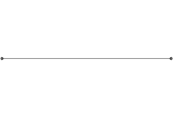
(a) The arc

(b) The $\sin(1/x)$-continuum

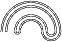
(c) Knaster bucket-handle

(d) A double bucket-handle

Figure 1. Some examples of arc-like continua; terminal points are marked by grey circles. (The numbers of terminal points in these continua are two, three, one and zero, respectively.)

We can now state our main theorem: The possible Julia continua of disjoint-type entire functions of bounded slope are precisely the arc-like continua having terminal points. The class of arc-like continua is extremely rich (e.g., there are uncountably many pairwise non-homeomorphic arc-like continua) and has been studied intensively by topologists since the work of Bing [Bin51b] in the 1950s. A few examples of arc-like continua and their terminal points are shown in Figure 1; for the formal definition and further discussion, see Definition 1 and Section 9 below.

3 Theorem (Topology of bounded-slope Julia continua).

Let $\hat{C}$ be a Julia continuum of a disjoint-type entire function $f$ of bounded slope. Then $\hat{C}$ is arc-like and $\infty$ is a terminal point of $\hat{C}$.

Conversely, there exists a disjoint-type entire function $f$ having bounded slope with the following property. If $X$ is any arc-like continuum having a terminal point $x\in X$, then there exists a Julia continuum $\hat{C}$ of $f$ and a homeomorphism $\psi\colon X\to\hat{C}$ such that $\psi(x)=\infty$.

Let us remark on a striking property of the function $f$ whose existence is asserted in Theorem 3. Suppose that $F_{\lambda}(x)=\lambda x(1-x)$ is a member of the famous logistic family of interval maps, for $\lambda\in[1,4]$. Then the inverse limit space of $F_{\lambda}$ – that is, the space of all backward orbits – is an arclike continuum having a terminal point (see Proposition 2). It is known [BBŠ12, Theorem 1.2] that the topology of this continuum determines $F_{\lambda}$ up to a natural notion of conjugacy. Hence the topology of $J(f)$, for the single disjoint-type function $f$, contains all information about the topological dynamics of all members of the logistic family.

In the case where $f$ does not have bounded slope (or even “anguine tracts”), we obtain the following result.

4 Theorem (Topology of Julia continua).

Let $\hat{C}$ be a Julia continuum of a disjoint-type entire function $f$. Then $\hat{C}$ has span zero and $\infty$ is a terminal point of $\hat{C}$.

Here “span zero” is another famous concept from continuum theory; again see Definition 1. It is well-known [Lel64] that every arc-like continuum has span zero. A long-standing question, posed by Lelek [Lel71, Problem 1] in 1971 and featured on many subsequent problem lists in topology, asked whether every continuum with span zero must be arc-like. This would imply that Theorem 3 gives a complete classification of Julia continua. However, Hoehn [Hoe11] constructed a counterexample to Lelek’s problem in 2011. The conjecture does hold when the continuum in question is either hereditarily decomposable  [Bin51b] or hereditarily indecomposable [HO16]; see Definition 13.

Since any Julia continuum different from those constructed in Theorem 3 would be of span zero but not arc-like, it would be of considerable topological interest. It is conceivable that one can construct a disjoint-type entire function having a Julia continuum of this type, thus yielding a new proof of Hoehn’s theorem mentioned above. We do not pursue this investigation here.

We prove a number of additional and more precise results, which are stated and discussed in Section 2. To conclude the introduction, we discuss the wider significance of the class of disjoint-type entire functions, and then mention two easily-stated important applications of our results and methods.

Significance of disjoint-type functions

In the study of dynamical systems, hyperbolic systems (also referred to as Axiom A, using Smale’s terminology) are those that exhibit the simplest behaviour; understanding the hyperbolic case is usually the first step in building a more general theory. Since entire functions of disjoint type are those hyperbolic functions that have the simplest combinatorial structure, their properties are of intrinsic interest, and their detailed understanding provides an important step towards understanding larger classes. However, our results also have direct consequences far beyond the disjoint-type case. Indeed, consider the Eremenko-Lyubich class

$$\mathcal{B}\mathrel{\vbox{\hbox{\scriptsize.}\hbox{\scriptsize.}}}=\{f\colon\mathbb{C}\to\mathbb{C}\text{ transcendental entire}\colon S(f)\text{ is bounded}\}.$$

By definition, this class contains all hyperbolic functions, as well as the particularly interesting Speiser class $\mathcal{S}$ of functions for which $S(f)$ is finite. We remark that, for $f\in\mathcal{B}$, always $I(f)\subset J(f)$ [EL92].

If $f\in\mathcal{B}$, then the map

(1.1) $$f_{\lambda}\colon\mathbb{C}\to\mathbb{C};\quad z\mapsto\lambda f(z)$$

is of disjoint type for sufficiently small $\lambda$ [Rem09, §5, p. 261]. If additionally the original function $f$ is hyperbolic, then by [Rem09, Theorem 5.2], the dynamics of $f$ on its Julia set $J(f)$ can be obtained, via a suitable semi-conjugacy, as a quotient of that of $f_{\lambda}$ on $J(f_{\lambda})$. This result has been generalised, first by Mihaljević-Brandt [Mih12] and more recently by Alhabib, Sixsmith and the author [ARS18] to important larger classes of entire functions (more precisely: geometrically finite entire functions whose local backward branches on the Julia set have uniformly bounded degree).

In each of these cases, the semi-conjugacy in question restricts to a homeomorphism on each connected component of $J(f_{\lambda})$. Hence all of our results concerning the topology of Julia components for the disjoint-type function $f_{\lambda}$ apply directly to the corresponding subsets of $J(f)$ also.

Furthermore, [BR17] introduces the notion of periodic “dreadlocks” – a generalisation of the above-mentioned “hairs” – for entire functions with bounded postsingular sets. This includes all hyperbolic functions, and more generally all geometrically finite entire functions. These dreadlocks promise to play an important role in the combinatorial study of class $\mathcal{B}$ entire functions; indeed, they have already been used to prove the existence and uniqueness of (homotopy) Hubbard trees for general post-singularly finite entire functions [Pfr19]. Our results on disjoint-type Julia continua apply directly to (landing) dreadlocks; indeed, any periodic dreadlock together with its landing point is homeomorphic to a corresponding component of $J(f_{\lambda})$, with $f_{\lambda}$ from (1.1) of disjoint type.

Yet more generally, for any $f\in\mathcal{B}$, it is shown in [Rem09, Theorem 1.1] that $f$ and the disjoint-type function $f_{\lambda}$ have the same dynamics near infinity. It follows that our results, which apply a priori only to the disjoint-type function $f_{\lambda}$, also have interesting consequences for general $f\in\mathcal{B}$.

Two applications

A famous example of a continuum (i.e., a non-empty compact, connected metric space) that contains no arcs is provided by the pseudo-arc (see Definition 1). The pseudo-arc is the unique hereditarily indecomposable arc-like continuum and has the intriguing property of being homeomorphic to each of its non-degenerate subcontinua. Theorem 3 shows that the pseudo-arc can arise in the Julia set of a transcendental entire function; as far as we are aware, this is the first time that a dynamically defined subset of the Julia set of an entire or meromorphic function has been shown to be a pseudo-arc. In fact, we show even more:

5 Theorem (Pseudo-arcs in Julia sets).

There exists a disjoint-type entire function $f\colon\mathbb{C}\to\mathbb{C}$ such that, for every connected component $C$ of $J(f)$, the set $C\cup\{\infty\}$ is a pseudo-arc.

Observe that this result sharpens the aforementioned [RRRS11, Theorem 8.4].

A further motivation for studying the topological dynamics of disjoint-type functions comes from a second question asked by Eremenko in [Ere89]: Is every connected component of $I(f)$ unbounded? This problem is now known as Eremenko’s Conjecture, and has remained open despite considerable attention. For disjoint-type maps, and indeed for any entire function with bounded postsingular set, it is known that the answer is positive [Rem07]. However, the disjoint-type case nonetheless has a role to play in the study of Eremenko’s Conjecture. Indeed, as discussed in [Rem09, Section 7], we may strengthen the question slightly by asking which entire functions have the following property:

1. For all $z\in I(f)$, there is a connected and unbounded set $A\subset\mathbb{C}$ with $z\in A$ such that $f^{n}|_{A}\to\infty$ uniformly.

If there exists a counterexample $f$ to Eremenko’s Conjecture in the class $\mathcal{B}$, then clearly $f$ cannot satisfy property (UE). In this case, it follows from [Rem09, p. 265] that (UE) fails for every map of the form $f_{\lambda}\mathrel{\vbox{\hbox{\scriptsize.}\hbox{\scriptsize.}}}=\lambda f$. As noted above, $f_{\lambda}$ is of disjoint type for $\lambda$ sufficiently small, so we see that any counterexample $f\in\mathcal{B}$ would need to be closely related to a disjoint-type function for which (UE) fails. The author suggested in [Rem07, Rem09] that it might be possible to construct such an example; in this article we realise this construction for the first time. Indeed, as we discuss in more detail in the next section, there is a surprisingly close relationship between the topology of the Julia set and the existence of points $z\in I(f)$ for which (UE) fails. Hence our results allow us to give a good description of the circumstances in which such points exist at all, which is likely to be important in any attempt to resolve Eremenko’s Conjecture. In particular, we can prove the following, which considerably strengthens the examples alluded to in [Rem07, Rem09].

6 Theorem (Non-uniform escape to infinity).

There is a disjoint-type entire function $f$ and an escaping point $z\in I(f)$ with the following property. If $A\subset I(f)$ is connected and $\{z\}\subsetneq A$, then

$$\liminf_{n\to\infty}\inf_{\zeta\in A}|f^{n}(\zeta)|<\infty.$$

2. Further discussion and results

In this section, we state and discuss further and more detailed results about the properties of Julia continua, going beyond those mentioned in the introduction. Let us begin by providing the formal definition of the concepts from continuum theory that have already been mentioned.

1 Definition (Terminal points; span zero; arc-like continua).

Let $X$ be a continuum; i.e. $X$ is a non-empty compact, connected metric space.

1. A point $x\in X$ is called a terminal point of $X$ if, for any two subcontinua $A,B\subset X$ with $x\in A\cap B$, either $A\subset B$ or $B\subset A$.

2. $X$ is said to have span zero if, for any subcontinuum $\mathcal{A}\subset X\times X$ whose first and second coordinates both project to the same subcontinuum $A\subset X$, $\mathcal{A}$ must intersect the diagonal. (I.e., if $\pi_{1}(\mathcal{A})=\pi_{2}(\mathcal{A})$, then there is $x\in X$ such that $(x,x)\in\mathcal{A}$.)

3. A non-degenerate continuum $X$ is said to be arc-like if, for every $\varepsilon>0$, there exists a continuous function $g\colon X\to[0,1]$ such that $\operatorname{diam}(g^{-1}(t))<\varepsilon$ for all $t\in[0,1]$.

4. $X$ is called a pseudo-arc if $X$ is arc-like and also hereditarily indecomposable (i.e., every point of $X$ is terminal).

For the benefit of those readers who have not encountered these concepts before, let us make a few comments regarding their meaning.

1. One should think of terminal points as a natural analogue of the endpoints of an arc. However, as the example of the pseudo-arc shows, a continuum may contain far more than two terminal points.

   We remark that there are several different and inequivalent notions of “terminal points” in use in continuum theory. The above definition can be found e.g. in [Fug66, Definition 3], and differs, in particular, from that of Miller [Mil50, p. 131]. On the other hand, the distinction is not essential for our purposes, since both notions coincide for the types of continua studied in this paper.

2. Roughly speaking, $X$ has span zero if two points cannot exchange their position by travelling within $X$ without meeting somewhere.

3. Intuitively, a continuum is arc-like if it looks like an arc when viewed at arbitrarily high, but finite, precision. As we discuss in Section 9, there are a number of equivalent definitions, the most important of which is that $X$ is arc-like if and only if it can be written as an inverse limit of arcs with surjective bonding maps.

4. Any two pseudo-arcs, as defined above, are homeomorphic [Bin51a, Theorem 1]; for this reason, we also speak about the pseudo-arc. We refer to Exercise 1.23 in [Nad92] for a construction that shows the existence of such an object, the introduction to Section 12 in the same book for a short history, and to [Lew99] for a survey of further results.

Nonescaping points and accessible points

Recall that Theorems 3 and 4 give an almost complete description of the possible topology of Julia continua. Let us now turn to the behaviour of points in a Julia continuum $\hat{C}=C\cup\{\infty\}$ under iteration. In the case of disjoint-type sine (or exponential) maps, and indeed for any disjoint-type entire function of finite order, each component $C$ of the Julia set is an arc and contains at most one point that does not tend to infinity under iteration, namely the finite endpoint of $C$. Furthermore, this finite endpoint is always accessible from the Fatou set of $f$; no other point can be accessible from $F(f)$. (Compare [DG87].) This suggests the following questions:

1. Can a Julia continuum contain more than one nonescaping point?

2. Is every nonescaping point accessible from $F(f)$?

3. Does every Julia continuum contain a point that is accessible from $F(f)$? This question is raised in [BK07, p. 393], where the authors prove that the answer is positive when a certain growth condition is imposed on the external address (see Definition 6) of the component $C$.

To answer these questions, we require one more topological concept.

2 Definition (Irreducibility).

Let $X$ be a continuum, and let $x_{0},x_{1}\in X$. We say that $X$ is irreducible between $x_{0}$ and $x_{1}$ if no proper subcontinuum of $X$ contains both $x_{0}$ and $x_{1}$.

We shall apply this notion only in the case where $x_{0}$ and $x_{1}$ are terminal points of $X$. In this case, irreducibility of $X$ between $x_{0}$ and $x_{1}$ means that, in some sense, the points $x_{0}$ and $x_{1}$ lie “on opposite ends” of $X$. For example, the $\sin(1/x)$-continuum of Figure 1LABEL:sub@subfig:sinecurve is irreducible between the terminal point on the right of the image and either of the two terminal points on the left, but not between the latter two (since the limiting interval is a proper subcontinuum containing both).

3 Theorem (Nonescaping and accessible points).

Let $\hat{C}$ be a Julia continuum of a disjoint-type entire function $f$. Any nonescaping point $z_{0}$ in $\hat{C}$ is a terminal point of $\hat{C}$, and $\hat{C}$ is irreducible between $z_{0}$ and $\infty$. The same is true for any point $z_{0}\in\hat{C}$ that is accessible from $F(f)$.

Furthermore, the set of nonescaping points in $\hat{C}$ has Hausdorff dimension zero. On the other hand, there exist a disjoint-type function having a Julia continuum for which the set of nonescaping points is a Cantor set and a disjoint-type function having a Julia continuum that contains a dense set of nonescaping points.

A Julia continuum contains at most one accessible point (see Theorem 10), so the two functions whose existence is asserted in Theorem 3 must have nonescaping points that are not accessible from $F(f)$. Furthermore, we can apply Theorem 3 to the bucket-handle continuum of Figure 1LABEL:sub@subfig:knaster, which has only a single terminal point. Hence the corresponding Julia continuum $\hat{C}$ (which, as discussed below, can be chosen such that the iterates do not converge uniformly to infinity on $C$) contains neither nonescaping nor accessible points. In particular, this answers the question of Barański and Karpińska.

We remark that it is also possible to construct an inaccessible Julia continuum that does contain a finite terminal point $z_{0}$. Indeed, we shall see that the examples mentioned in the second half of the preceding theorem must have this property (compare the remark after Theorem 10). Alternatively, such an example could be achieved by ensuring that the continuum is embedded in the plane in such a way that $z_{0}$ is not accessible from the complement of $\hat{C}$ (see Figure 2); we do not discuss the details here.

Bounded-address and periodic Julia continua

We now turn our attention to the different types of dynamics that $f$ can exhibit on a Julia continuum. In Theorem 3, we saw that, given any arc-like continuum $X$ having a terminal point, there are a disjoint-type function $f$ and a Julia continuum $\hat{C}$ of $f$ such that $\hat{C}$ is homeomorphic to $X$. We shall see that it is possible to choose $\hat{C}=C\cup\{\infty\}$ either such that $f^{n}|_{C}\to\infty$ uniformly, or such that $\min_{z\in C}|f^{n}(z)|<R$ for some $R>0$ and infinitely many $n$. However, our construction will always lead to continua with $\limsup_{n\to\infty}\min_{z\in C}|f^{n}(z)|=\infty$. In particular, the Julia continuum cannot be periodic.

Periodic points, and periodic continua consisting of escaping points, play a crucial role in complex dynamics. Hence it is interesting to consider when we can improve on the preceding results, in the following sense.

4 Definition (Periodic and bounded-address Julia continua).

Let $\hat{C}=C\cup\{\infty\}$ be a Julia continuum of a disjoint-type function $f$. We say that $\hat{C}$ is periodic if $f^{n}(C)=C$ for some $n\geq 1$.

We also say that $\hat{C}$ has bounded address if there is $R>0$ such that, for every $n\in\mathbb{N}$, there exists a point $z\in C$ such that $|f^{n}(z)|\leq R$.

Upon reflection, it becomes evident that not every arc-like continuum $X$ having a terminal point can arise as a Julia continuum with bounded address. Indeed, it is well-known that every Julia continuum $\hat{C}$ at bounded address contains a unique point with a bounded orbit, and hence that every periodic Julia continuum contains a periodic point. (See Proposition 10.) In particular, by Theorem 3, $\hat{C}$ contains some terminal point $z_{0}$ such that $\hat{C}$ is irreducible between $z_{0}$ and $\infty$. So if $X$ is an arc-like continuum that does not contain two terminal points between which $X$ is irreducible (such as the Knaster buckethandle), then $X$ cannot be realised by a bounded-address Julia continuum. It turns out that this is the only restriction.

5 Theorem (Classification of bounded-address Julia continua).

There exists a disjoint-type entire function $f$ having bounded slope with the following property.

Let $X$ be an arc-like continuum, and let $x_{0},x_{1}\in X$ be two terminal points between which $X$ is irreducible. Then there is a Julia continuum $\hat{C}$ of $f$ with bounded address and a homeomorphism $\psi\colon X\to\hat{C}$ such that $\psi(x_{0})$ has bounded orbit under $f$ and such that $\psi(x_{1})=\infty$.

We also observe that not every continuum $X$ as in Theorem 5 can occur as a periodic Julia continuum. Indeed, if $\hat{C}$ is a periodic Julia continuum, then $f^{p}\colon\hat{C}\to\hat{C}$ is a homeomorphism, where $p$ is the period of $\hat{C}$, and $f^{p}$ is extended to $\hat{C}$ by setting $f^{p}(\infty)=\infty$. Furthermore, all points of $\hat{C}$ but one tend to $\infty$ under iteration by $f^{p}$. However, if $X$ is, say, the $\sin(1/x)$-continuum from Figure 1, then every self-homeomorphism of $X$ must map the limiting interval on the left to itself. Hence there cannot be any periodic Julia continuum $\hat{C}$ that is homeomorphic to $X$. The correct class of continua for this setting was discussed by Rogers [Rog70] in 1970.

6 Definition (Rogers continua).

Let $X$ be homeomorphic to the inverse limit of a surjective continuous self-map $h$ of the interval $[0,1]$ with $h(t)<t$ for $0<t<1$, and let $x_{0}$ and $x_{1}$ denote the points of $X$ corresponding to $0\mapsfrom 0\mapsfrom 0\dots$ and $1\mapsfrom 1\mapsfrom\dots$. Then we shall say that $X$ is a Rogers continuum (from $x_{0}$ to $x_{1}$).

2.1 Remark.

The inverse limit generated by $h$ is the space of all backward orbits of $h$, equipped with the product topology (Definition 15).

7 Theorem (Periodic Julia continua).

Let $X$ be a continuum and let $x_{0},x_{1}\in X$. Then the following are equivalent:

1. $X$ is a Rogers continuum from $x_{0}$ to $x_{1}$.

2. There exists a disjoint-type entire function $f$ of bounded slope, a periodic Julia continuum $\hat{C}$ of $f$, say of period $p$, and a homeomorphism $\psi\colon X\to\hat{C}$ such that $f^{p}(\psi(x_{0}))=\psi(x_{0})$ and $\psi(x_{1})=\infty$.

2.2 Remark (Remark 1).

Both Theorem 5 and the combination of Theorems 3 and 4 can be stated in the following form: Any (resp. any bounded-address) Julia continuum (whether arc-like or not) has a certain intrinsic topological property $\mathcal{S}$, and any arc-like continuum with property $\mathcal{S}$ can be realised as a Julia continuum (resp. bounded-address Julia continuum) of a disjoint-type, bounded-slope entire function. Rogers’s result in [Rog70] gives such a description also for Theorem 7, assuming additionally that $X$ is decomposable. It is an interesting question whether this can be achieved also in the indecomposable case, although we note that there is no known intrinsic topological description of those arc-like continua that can be written as an inverse limit with a single bonding map.

2.3 Remark (Remark 2).

Another difference between Theorem 7 and Theorems 3 and 5 is that not all Rogers continua can be realised by the same function. Indeed, it can be shown that there are uncountably many pairwise non-homeomorphic Rogers continua, while the set of periodic Julia continua of any given function is countable.

2.4 Remark (Remark 3).

By a classical result of Henderson [Hen64], the pseudo-arc is a Rogers continuum (where $x_{0}$ and $x_{1}$ can be taken as any two points between which it is irreducible). Hence we see from Theorem 7 that it can arise as an invariant Julia continuum of a disjoint-type entire function. It follows from the nature of our construction in the proof of Theorem 7 that, in this case, all Julia continua are pseudo-arcs (see Corollary 8), establishing Theorem 5 as stated in the introduction.

(Non-)uniform escape to infinity

We now return to the question of rates of escape to infinity, and the “uniform Eremenko property” (UE). Recall that by Theorem 3 it is possible to construct a Julia continuum $\hat{C}$ that contains no finite terminal points, and hence has the property that $C\subset I(f)$ by Theorem 3. Also recall that we can choose $\hat{C}$ in such a way that the iterates of $f$ do not tend to infinity uniformly on $C$. This easily implies that there is some point in $C$ for which the property (UE) fails.

To study this type of question in greater detail, we introduce the following natural definition.

8 Definition (Escaping composants).

Let $f$ be a transcendental entire function, and let $z\in I(f)$. The escaping composant $\mu(z)$ is the union of all connected sets $A\ni z$ such that $f^{n}|_{A}\to\infty$ uniformly.

We also define $\mu(\infty)$ to be the union of all unbounded connected sets $A$ such that $f^{n}|_{A}\to\infty$ uniformly.

With this definition, property (UE) requires precisely that $I(f)=\mu(\infty)$. For a disjoint-type entire function, it makes sense to study this property separately for each Julia continuum $\hat{C}$; i.e. to ask whether all escaping points in $\hat{C}$ belong to $\mu(\infty)$. Clearly this is the case by definition when $f^{n}\to\infty$ uniformly on $C=\hat{C}\setminus\{\infty\}$. Otherwise, it turns out that there is a close connection between the above question and the topology of $\hat{C}$. Recall that the (topological) composant of a point $x_{0}$ in a continuum $X$ is the union of all proper subcontinua of $X$ containing $x_{0}$. The topological composant of $\infty$ in a Julia continuum $\hat{C}$ is always a proper subset of $\hat{C}$, since $\infty$ is a terminal point.

9 Theorem (Topological composants and escaping composants).

Let $\hat{C}=C\cup\{\infty\}$ be a Julia continuum of a disjoint-type entire function, and suppose that $f^{n}|_{C}$ does not tend to infinity uniformly. Then the topological composant of $\infty$ in $\hat{C}$ is given by $\{\infty\}\cup(\mu(\infty)\cap C)$.

If $\hat{C}$ is periodic, then $\hat{C}$ is indecomposable if and only if $C\cap I(f)\setminus\mu(\infty)\neq\emptyset$ (that is, if $C$ contains an escaping point for which property (UE) fails).

Any indecomposable continuum has uncountably many composants, all of which are pairwise disjoint. Hence we see that complicated topology of non-uniformly escaping Julia continua automatically leads to the existence of points that cannot be connected to infinity by a set that escapes uniformly. However, our proof of Theorem 3 also allows us to construct Julia continua that have very simple topology, but nonetheless contain points in $I(f)\setminus\mu(\infty)$.

10 Theorem (A one point escaping composant).

There exists a disjoint-type entire function $f$ and a Julia continuum $\hat{C}=C\cup\{\infty\}$ of $J(f)$ such that:

1. $\hat{C}$ is an arc, with one finite endpoint $z_{0}$ and one endpoint at $\infty$;

2. $C\subset I(f)$, but $\liminf_{n\to\infty}\min_{z\in C}|f^{n}(z)|<\infty$. In particular, there is no non-degenerate connected set $A\ni z_{0}$ on which the iterates escape to infinity uniformly.

Observe that this implies Theorem 6.

Number of tracts and singular values

So far, we have not said much about the nature of the functions $f$ that occur in our examples, except that they are of disjoint type. Using recent results of Bishop [Bis15a, Bis15b, Bis17], we can say considerably more:

11 Theorem (Class $\mathcal{S}$ and number of tracts).

All examples of disjoint-type entire functions $f$ mentioned in the introduction and in this section can be constructed in such a way that $f$ has exactly two critical values and no finite asymptotic values, and such that all critical points of $f$ have degree at most $16$.

Furthermore, with the exception of Theorem 5, the function $f$ can be constructed such that

$$\mathcal{T}_{R}\mathrel{\vbox{\hbox{\scriptsize.}\hbox{\scriptsize.}}}=f^{-1}(\{z\in\mathbb{C}\colon|z|>R\})$$

is connected for all $R$. In Theorem 5, the function $f$ can be constructed so that $\mathcal{T}_{R}$ has exactly two connected components for sufficiently large $R$.

2.5 Remark (Remark 1).

On the other hand, if $\mathcal{T}_{R}$ is connected for all $R$, then it turns out that every Julia continuum at a bounded address is homeomorphic to a periodic Julia continuum (Proposition 1). Hence it is indeed necessary to allow $\mathcal{T}_{R}$ to have two components in Theorem 5.

2.6 Remark (Remark 2).

The bound of $16$ on the degree of critical points can be reduced to $4$ by modifying Bishop’s construction; compare Remark 2

As pointed out in [BFR14], this leads to an interesting observation. By Theorem 11, the function $f$ from Theorem 5 can be constructed such that $\#S(f)=2$, such that $f$ has no asymptotic values and such that all critical points have degree at most $16$. Let $v_{1}$ and $v_{2}$ be the critical values of $f$, and let $c_{1}$ and $c_{2}$ be critical points of $f$ over $v_{1}$ resp. $v_{2}$. Let $A\colon\mathbb{C}\to\mathbb{C}$ be the affine map with $A(v_{1})=c_{1}$ and $A(v_{2})=c_{2}$. Then the function $g\mathrel{\vbox{\hbox{\scriptsize.}\hbox{\scriptsize.}}}=f\circ A$ has super-attracting fixed points at $v_{1}$ and $v_{2}$. By the results from [Rem09] discussed earlier, the Julia set $J(g)$ contains uncountably many invariant subsets for each of which the one-point compactification is a pseudo-arc. On the other hand, $J(g)$ is locally connected by [BFR14, Corollary 1.9]. Hence we see that, in contrast to the polynomial case, local connectivity of Julia sets does not imply simple topological dynamics, even for hyperbolic functions. Compare [Roe08] for a similar phenomenon in the case of (albeit non-hyperbolic) rational maps.

Embeddings

Given an arc-like continuum $X$, there are usually different ways to embed $X$ in the Riemann sphere $\hat{\mathbb{C}}$. That is, there might be continua $C_{1},C_{2}\subset\hat{\mathbb{C}}$ such that $X$ is homeomorphic to $C_{1}$ and $C_{2}$, but such that no homeomorphism $\hat{\mathbb{C}}\to\hat{\mathbb{C}}$ can map $C_{1}$ to $C_{2}$. (That is, $C_{1}$ and $C_{2}$ are not ambiently homeomorphic.) Our construction in the proof of Theorem 3 is rather flexible, and we could indeed use it to construct different Julia continua that are homeomorphic but not ambiently homeomorphic. In particular, as briefly mentioned already in the discussion of results concerning accessibility, it would be possible to construct a Julia continuum $\hat{C}$ that is homeomorphic to the $\sin(1/x)$-continuum, and such that the limiting arc is not accessible from the complement of $\hat{C}$. (See Figure 2).

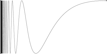
(a)

(b)

Figure 2. Two embeddings of the $\sin(1/x)$-continuum that are not ambiently homeomorphic

It is easy to see that, for a disjoint-type entire function which has bounded slope, every Julia continuum can be covered by a chain with arbitrarily small links such that every link is a connected subset of the Riemann sphere. (For the definition of a chain, compare the remark after Proposition 2.) It is well-known [Bin51b, Example 3] that there are embeddings of arc-like continua without this property. It is natural to ask whether this is the only restriction on the continua that can arise by our construction, but we shall defer this and similar problems to future investigations.

Structure of the article

In Section 3, we collect background on the dynamics of disjoint-type entire functions. In particular, we review the logarithmic change of variable, which is used throughout the remainder of the paper. We also recall some basic facts from the theory of continua. Section 4 discusses a general conjugacy principle between expanding inverse systems, which will be useful throughout. Following these preliminaries, the article essentially splits into two parts, which can largely be read independently of each other:

• General topology of Julia continua. We first study general properties of Julia continua of disjoint-type entire functions. More precisely, in Section 5 we show that each such continuum has span zero, and prove the various results concerning terminal points stated earlier; in particular, we establish Theorem 4. In Section 6, we investigate the structure of escaping composants. Section 7 studies conditions under which all Julia continua are arclike, and establishes one half of Theorem 7. Finally, Section 8 shows that, in certain circumstances, different Julia continua are homeomorphic to each other. These results show that our constructions in the second part of the paper are optimal in a certain sense, and are also used in the proof of Theorem 5.

• Constructing prescribed Julia continua. The second part of the paper is concerned with constructions that allow us to find entire functions having prescribed arc-like Julia continua, as outlined in the theorems stated in the introduction and the present section. We review topological background on arc-like continua in Section 9 and, in Section 10, give a detailed proof of a slightly weaker version of Theorem 3 (where the function $f$ is allowed to depend on the arc-like continuum in question). Section 11 applies this general construction to obtain the examples from Theorems 6, 10 and 3, and the proof of Theorem 3 is completed in Section 12. Section 13 discusses the modification of the construction from Section 10 necessary to obtain bounded-address continua for Theorem 5. Section 14 contains the proofs of Theorems 7 and 5. Finally, we briefly discuss how to modify the constructions to obtain Theorem 11 (Section 15).

Basic notation

As usual, we denote the complex plane by $\mathbb{C}$ and the Riemann sphere by $\hat{\mathbb{C}}$. We also denote the unit disk by $\mathbb{D}$ and the right half-plane by $\mathbb{H}$. All boundaries and closures of plane sets will be understood to be taken in $\mathbb{C}$, unless explicitly noted otherwise.

We shall also continue to use the notations introduced throughout Sections 1 and 2. In particular, the Fatou, Julia and escaping sets of an entire function are denoted by $F(f)$, $J(f)$ and $I(f)$, respectively. Euclidean distance is denoted by $\operatorname{dist}$.

In order to keep the paper accessible to readers with a background in either continuum theory or transcendental dynamics, but not necessarily both, we aim to introduce all notions and results required from either area. For further background on transcendental iteration theory, we refer to [Ber93]. For a wealth of information on continuum theory, including the material treated here, we refer to [Nad92]. In particular, a detailed treatment of arc-like continua can be found in [Nad92, Chapter 12].

We shall assume that the reader is familiar with plane hyperbolic geometry; see e.g. [BM07]. If $U\subset\mathbb{C}$ is simply-connected, then we denote the density of the hyperbolic metric by $\rho_{U}\colon U\to(0,\infty)$. In particular, we shall frequently use the standard estimate on the hyperbolic metric in a simply-connected domain [BM07, Theorems 8.2 and 8.6]:

(2.1) $$\frac{1}{2\operatorname{dist}(z,\partial U)}\leq\rho_{U}(z)\leq\frac{2}{\operatorname{dist}(z,\partial U)}.$$

If $U$ is disjoint from its translates by integer multiples of $2\pi i$, then $\operatorname{dist}(z,\partial U)\leq\pi$ for all $z\in U$. Thus (2.1) yields what we shall call the standard bound for logarithmic tracts:

(2.2) $$\rho_{U}(z)\geq\frac{1}{2\pi}.$$

We also denote hyperbolic diameter in $U$ by $\operatorname{diam}_{U}$, and hyperbolic distance by $\operatorname{dist}_{U}$. Furthermore, the derivative of a holomorphic function $f$ with respect to the hyperbolic metric is denoted by $\|{\rm D}f(z)\|_{U}$. (Note that this is defined whenever $z,f(z)\in U$.)

Acknowledgements

I am extremely grateful to Mashael Alhamd, Patrick Comdühr, Alexandre DeZotti, Leticia Pardo Simón, Dave Sixsmith and Stephen Worsley for the careful reading of the manuscript and many thoughtful comments, questions and suggestions for improvement. I would also like to thank Anna Benini, Chris Bishop, Clinton Curry, Toby Hall, Daniel Meyer, Phil Rippon and Gwyneth Stallard for interesting and stimulating discussions regarding the reported research.

3. Preliminaries

Disjoint-type entire functions

Let $f\colon\mathbb{C}\to\mathbb{C}$ be a transcendental entire function. Recall that $f$ is said to be of disjoint type if it is hyperbolic with connected Fatou set. As far as we are aware, this class of functions was first studied by Barański and Karpińska [BK07]. The material in this section is not new, but is taken from different papers with sometimes conflicting notation. For this reason we give a consistent account tailored to our purposes; we include (sketches of) proofs where these are relevant for the applications that follow.

The following (see [BK07, Lemma 3.1] or [Mih12, Proposition 2.8]) provides an alternative definition, which is the one that we shall work with.

1 Proposition (Characterization of disjoint-type functions).

A transcendental entire function $f\colon\mathbb{C}\to\mathbb{C}$ is of disjoint type if and only if there exists a bounded Jordan domain $D$ with $S(f)\subset D$ and $f(\overline{D})\subset D$.

Let $f$ be of disjoint type, and consider the domain $W\mathrel{\vbox{\hbox{\scriptsize.}\hbox{\scriptsize.}}}=\mathbb{C}\setminus\overline{D}$, with $D$ as in Proposition 1. Since $S(f)\cap W=\emptyset$, if $V$ is any connected component of $\mathcal{V}\mathrel{\vbox{\hbox{\scriptsize.}\hbox{\scriptsize.}}}=f^{-1}(W)$, then $f\colon V\to W$ is a covering map. These components are called the tracts of $f$ (over $\infty$). Note that the disjoint-type condition implies that the boundaries $\partial W$ and $\partial\mathcal{V}$ are disjoint; this is the reason for our choice of terminology.

Since $f$ is transcendental, it follows from the classification of covering maps of the punctured disc [For99, Theorem 5.10] that every tract $V$ is simply-connected and unbounded, and that $f\colon V\to W$ is a universal covering map. Observe that a slightly smaller domain $\widetilde{D}$ (with closure contained in $D$) still satisfies the conclusions of Proposition 1. Applying the above observations to $\widetilde{D}$ and the resulting collection of tracts $\widetilde{\mathcal{V}}$, we can deduce that the boundary of any connected component $V$ of $\mathcal{V}$ is the preimage of the simple closed curve $\partial D$ under a universal covering map. Hence $V$ is an unbounded Jordan domain, i.e. a simply-connected domain whose boundary in $\hat{\mathbb{C}}$ is a simple closed curve passing through $\infty$. Furthermore, different tracts have disjoint closures, as every component of the open set $\widetilde{\mathcal{V}}$ contains the closure of exactly one tract $V$. Furthermore, any compact set $K$ intersects at most finitely many tracts (since $\widetilde{\mathcal{V}}$ is an open cover of $K\cap\overline{\mathcal{V}}$).

The following characterises the Julia set of a disjoint-type entire function; for readers who are unfamiliar with transcendental dynamics, it may alternatively serve as the definition of the Julia set in this setting.

2 Proposition (Julia sets).

If $f$ is of disjoint type and $D$ is as in Proposition 1, then

$$J(f)=\{z\in\mathbb{C}\colon f^{n}(z)\notin\overline{D}\text{ for all $n\geq 0$}\}.$$

3.1 Proof.

Since $f$ is hyperbolic and of disjoint type, $F(f)$ is the immediate basin of attraction of a fixed point $p$. Since $f(\overline{D})\subset D$, we have $\overline{D}\subset F(f)$ and $p\in D$. Thus a point $z$ belongs to $F(f)$ if and only if its orbit eventually enters $\overline{D}$, as claimed.

The logarithmic change of variable

Following Eremenko and Lyubich, we study $f$ using the logarithmic change of variable [EL92, Section 2]. To this end, let us assume for simplicity that $0\in D$, which can always be achieved by conjugating $f$ with a translation. Set $H\mathrel{\vbox{\hbox{\scriptsize.}\hbox{\scriptsize.}}}=\exp^{-1}(W)$ and $\mathcal{T}\mathrel{\vbox{\hbox{\scriptsize.}\hbox{\scriptsize.}}}=\exp^{-1}(\mathcal{V})$. Since $0\notin W\supset\mathcal{V}$, and since $f$ is a universal covering on each tract, there is a holomorphic function $F\colon\mathcal{T}\to H$ such that $f\circ\exp=\exp\circ F$. We may choose this map $F$ to be $2\pi i$-periodic, in which case we refer to it as a logarithmic transform of $f$.

This representation is extremely convenient: for every component $T$ of $\mathcal{T}$, the map $F\colon T\to H$ is a conformal isomorphism, rather than a universal covering map as in the original coordinates. This makes it much easier to consider inverse branches. From now on, we shall always study the logarithmic transform of $f$. In fact, it is rather irrelevant for further considerations that the map $F$ has arisen from a globally defined entire function. This leads us to work in the following greater generality from now on.

3 Definition (The classes $\mathcal{B}_{\log}$ and $\mathcal{B}_{\log}^{\operatorname{p}}$ [Rem09, RRRS11]).

The class $\mathcal{B}_{\log}$ consists of all holomorphic functions

$$F\colon\mathcal{T}\to H,$$

where $F$, $\mathcal{T}$ and $H$ have the following properties:

1. $H$ is a $2\pi i$-periodic unbounded Jordan domain that contains a right half-plane.

2. $\mathcal{T}\neq\emptyset$ is $2\pi i$-periodic and $\operatorname{Re}z$ is bounded from below in $\mathcal{T}$, but unbounded from above.

3. Every connected component $T$ of $\mathcal{T}$ is an unbounded Jordan domain that is disjoint from all its $2\pi i\mathbb{Z}$-translates. For each such $T$, the restriction $F\colon T\to H$ is a conformal isomorphism whose continuous extension to the closure of $T$ in $\hat{\mathbb{C}}$ satisfies $F(\infty)=\infty$, and whose inverse we denote by $F_{T}^{-1}\mathrel{\vbox{\hbox{\scriptsize.}\hbox{\scriptsize.}}}=(F|_{T})^{-1}$. Each such component $T$ is called a tract of $F$.

4. The tracts of $F$ have pairwise disjoint closures and accumulate only at $\infty$; i.e., if $z_{n}\in\mathcal{T}$ is a sequence of points all belonging to different tracts of $F$, then $z_{n}\to\infty$.

If furthermore $F$ is $2\pi i$-periodic, then we say that $F$ belongs to the class $\mathcal{B}_{\log}^{\operatorname{p}}$. If $\overline{\mathcal{T}}\subset H$, then we say that $F$ is of disjoint type. If $F\in\mathcal{B}_{\log}$ is of disjoint type, then the Julia set and escaping set of $F$ are defined by

$$J(F)\mathrel{\vbox{\hbox{\scriptsize.}\hbox{\scriptsize.}}}=\ \{z\in H\colon F^{n}(z)\text{ is defined for all $n\geq 0$}\}$$

$$=\ \bigcap_{n\geq 0}F^{-n}(\overline{\mathcal{T}})\qquad\text{and}$$

$$I(F)\mathrel{\vbox{\hbox{\scriptsize.}\hbox{\scriptsize.}}}=\ \{z\in J(F)\colon\operatorname{Re}F^{n}(z)\to\infty\text{ as $n\to\infty$}\}.$$

3.2 Remark (Remark 1).

If $F\in\mathcal{B}_{\log}$ has disjoint type, then, by conjugation with an isomorphism $H\to\mathbb{H}$ that commutes with translation by $2\pi i$, we obtain a disjoint-type function $G\in\mathcal{B}_{\log}$ that is conformally conjugate to $F$ and whose range is the right half-plane $\mathbb{H}$. It is not difficult to see that all geometric properties discussed in this paper, such as bounded slope, are invariant under this transformation. Hence we could always assume that $H=\mathbb{H}$ in the following; this is the approach taken by Barański and Karpińska [BK07, Section 3]. However, we prefer to work directly with the above more general class, which retains a more direct connection to the original entire functions.

3.3 Remark (Remark 2).

Observe that the final condition d can be equivalently rephrased as follows:

1. The tracts of $F$ have pairwise disjoint closures. Furthermore, for every $R>0$, there are only finitely many tracts of $F$, up to translations by integer multiples of $2\pi i$, that intersect the vertical line at real part $R$.

In view of the preceding remark, we record the following observation, which will be used a number of times in the article.

4 Observation (Points to the left of a given line).

Let $F\colon\mathcal{T}\to H$ in $\mathcal{B}_{\log}$ be of disjoint type. Then for every $R>0$, there exists a constant $\Delta>0$ with the following property.

Let $T$ be a tract of $F$, let $T_{>R}$ be the unbounded connected component of the set $\{z\in T\colon\operatorname{Re}z>R\}$, and write $T_{\leq R}\mathrel{\vbox{\hbox{\scriptsize.}\hbox{\scriptsize.}}}=T\setminus T_{>R}\supset\{z\in T\colon\operatorname{Re}z\leq R\}$. Then $T_{\leq R}$ has diameter at most $\Delta$, both in the Euclidean metric and in the hyperbolic metric of $H$.

Furthermore, for every $R>0$ there is $M>0$ such that, for every $z\in H$:

$$\operatorname{diam}_{H}(\{w\in\mathcal{T}\colon|z-w|\leq R\})\leq M.$$

3.4 Proof.

Let us fix $R>0$. For a fixed tract $T$, the set $T_{\leq R}$ is compactly contained in $H$, and hence has finite Euclidean and hyperbolic diameter. Clearly $\tilde{T}_{\leq R}$ has the same diameter as $T_{R}$ if $\tilde{T}$ is a $2\pi i\mathbb{Z}$-translations of $T$. By property (d’) above, up to translations from $2\pi i\mathbb{Z}$, there are only finitely many tracts for which $T_{\leq R}\neq\emptyset$. This proves the first claim.

Furthermore, since $\overline{\mathcal{T}}\subset H$, and both $\mathcal{T}$ and $H$ are $2\pi i$-periodic, $\operatorname{dist}(z,\partial H)$ is uniformly bounded on $\mathcal{T}$. By the standard estimate (2.1), the density $\rho_{H}(z)$ is bounded from above, and the second claim follows.

Any logarithmic transform $F$ of a disjoint-type entire function, as described above, belongs to the class $\mathcal{B}_{\log}^{\operatorname{p}}$ and has disjoint type. The following theorem, which follows from recent ground-breaking work of Bishop [Bis15b, Bis17] together with the results of [Rem09], shows essentially that the converse also holds.

5 Theorem (Realisation of disjoint-type models).

Let $G\in\mathcal{B}_{\log}^{\operatorname{p}}$ be of disjoint type and let $g$ be defined by $g(\exp(z))=\exp(G(z))$. Then there exists a disjoint-type function $f\in\mathcal{B}$ such that $f|_{J(f)}$ is topologically (and, in fact, quasiconformally) conjugate to $g|_{\exp(J(G))}$.

Furthermore, there is a disjoint-type function $\tilde{f}\in\mathcal{S}$ such that every connected component of $J(G)$ is homeomorphic to a connected component of $J(\tilde{f})$ (but not necessarily vice-versa). The function $\tilde{f}$ may be chosen to have exactly two critical values, no asymptotic values, and no critical points of degree greater than $12$.

3.5 Proof.

The first statement is [Bis15b, Theorem 1.2], which is a consequence of Theorem 1.1 in the same paper and [Rem09, Theorem 3.1]. The second statement is [Bis17, Thoerem 1.5], which similarly follows from [Bis17, Theorem 1.2] and [Rem09].

Hence, in order to construct the examples of disjoint-type entire functions described in Sections 1 and 2, apart from the more precise statement in Theorem 11, it will be sufficient to construct functions in the class $\mathcal{B}_{\log}^{\operatorname{p}}$ with the analogous properties. (With some extra care, the construction of these examples in the class $\mathcal{B}$ could also be carried out using the earlier approximation result in [Rem13, Theorem 1.9], rather than the results of [Bis15b].) By nature of the construction, the approximation will also preserve certain geometric properties, such as the bounded-slope condition; compare Remark 3.

The same examples can be constructed in the class $\mathcal{S}$ using the second half of the above theorem, but in this case the entire functions will generally acquire additional tracts when compared with the original $\mathcal{B}_{\log}^{\operatorname{p}}$ models. (More precisely, they will have twice as many tracts as the original model.) In order to construct functions in the class $\mathcal{S}$ with the number of tracts stated in Theorem 11, we shall instead use Bishop’s more precise methods in [Bis15a] in Section 15.

The combinatorics of Julia continua

Let $F\in\mathcal{B}_{\log}^{\operatorname{p}}$ be of disjoint type. The tracts of $F$ and their iterated preimages provide successively finer partitions of $J(F)$, leading to a natural notion of symbolic dynamics as follows.

6 Definition (External addresses and Julia continua).

Let $F\in\mathcal{B}_{\log}$ have disjoint type. An external address of $F$ is a sequence $\underline{s}=T_{0}T_{1}T_{2}\dots$ of tracts of $F$.

If $\underline{s}$ is such an external address, then we define

$$J_{\underline{s}}(F)\mathrel{\vbox{\hbox{\scriptsize.}\hbox{\scriptsize.}}}=\ \{z\in J(F)\colon F^{n}(z)\in T_{n}\text{ for all $n\geq 0$}\}$$

$$=\ \{z\in J(F)\colon F^{n}(z)\in\overline{T_{n}}\text{ for all $n\geq 0$}\},$$

$$\hat{J}_{\underline{s}}(F)\mathrel{\vbox{\hbox{\scriptsize.}\hbox{\scriptsize.}}}=\ J_{\underline{s}}(F)\cup\{\infty\}\qquad\text{and}$$

$$I_{\underline{s}}(F)\mathrel{\vbox{\hbox{\scriptsize.}\hbox{\scriptsize.}}}=\ I(F)\cap J_{\underline{s}}(F).$$

When $J_{\underline{s}}(F)$ is nonempty, we say that $\underline{s}$ is admissible (for $F$). In this case, $\hat{J}_{\underline{s}}(F)$ is called a Julia continuum of $F$. An address $\underline{s}$ is called bounded if it contains only finitely many different tracts, and periodic if there is $p\geq 1$ such that $T_{j}=T_{j+p}$ for all $j\geq 0$.

For $n\geq m\geq 0$, we also define

$$F^{m\dots n}_{\underline{s}}\mathrel{\vbox{\hbox{\scriptsize.}\hbox{\scriptsize.}}}=F|_{T_{n}}\circ F|_{T_{n-1}}\circ\dots\circ F|_{T_{m}},\qquad F^{n}_{\underline{s}}\mathrel{\vbox{\hbox{\scriptsize.}\hbox{\scriptsize.}}}=F^{0\dots n-1}_{\underline{s}}\qquad\text{and}\qquad F^{-n}_{\underline{s}}\mathrel{\vbox{\hbox{\scriptsize.}\hbox{\scriptsize.}}}=(F^{n}_{\underline{s}})^{-1}.$$

3.6 Remark (Remark 1).

We can write $\hat{J}_{\underline{s}}(F)$ as a nested intersection of continua:

(3.1) $$\hat{J}_{\underline{s}}(F)=\bigcap_{n=0}^{\infty}\bigl{(}F_{\underline{s}}^{-n}(\overline{T_{n}})\cup\{\infty\}\bigr{)}.$$

Hence $\hat{J}_{\underline{s}}$ is indeed a continuum. Furthermore, if $\underline{s}^{1}\neq\underline{s}^{2}$, then for some $n\geq 0$, the sets $J_{\underline{s}^{1}}(F)$ and $J_{\underline{s}^{2}}(F)$ belong to different connected components of the open set $F^{-n}(\mathcal{T})$ (where $\mathcal{T}$ again denotes the domain of $F$). Hence every connected component of $J(F)$ is contained in a single Julia continuum.

3.7 Remark (Remark 2).

In [BK07, Remark after Theorem C’], the question is raised whether each $J_{\underline{s}}(F)$ is connected. It follows from [Rem07, Corollary 3.6] that this is indeed the case; compare the remark after Definition 1. We reprove this fact in Theorem 7, by showing that $\infty$ is a terminal point of $\hat{J}_{\underline{s}}(F)$. Indeed, a terminal point of a continuum $X$ cannot be a cut point of $X$ (this follows e.g. from the Boundary Bumping Theorem 12 below), so $J_{\underline{s}}(F)=\hat{J}_{\underline{s}}(F)\setminus\{\infty\}$ is connected.

In particular, if $f$ is an entire function of disjoint type and $F\in\mathcal{B}_{\log}^{\operatorname{p}}$ is a logarithmic transform of $f$, then every (arbitrary/bounded-address/periodic) Julia continuum of $f$, as defined in the introduction, is homeomorphic (via a branch of the logarithm) to a Julia continuum of $F$ at an (admissible/bounded/periodic) address, and vice versa.

3.8 Remark (Remark 3).

Recall that $F|_{T}$ extends continuously to $\infty$ with $F(\infty)=\infty$, for all tracts $T$ of $F$. Hence, throughout the article, we shall use the convention that $F(\infty)=\infty$. We emphasise that, while this extension is continuous on a given tract, and hence on a given Julia continuum, it is not a continuous extension of the global function $F$. When considering subsets of $\overline{T}\cup\{\infty\}$, it will also be convenient to use the convention that $\operatorname{Re}\infty=\infty$.

Hyperbolic expansion

In order to study disjoint-type functions, we shall use the fact that they are expanding on the Julia set, with respect to the hyperbolic metric on $H$. Recall that $\|{\rm D}F(z)\|_{H}$ denotes the hyperbolic derivative of $F$, measured in the hyperbolic metric of $H$, and that $\operatorname{diam}_{H}$ denotes hyperbolic diameter in $H$.

7 Proposition (Expanding properties of $F$).

Let $F\colon\mathcal{T}\to H$ be a disjoint-type function in $\mathcal{B}_{\log}$. Then there is a constant $\Lambda>1$ such that

$$\|{\rm D}F(z)\|_{H}\geq\Lambda,$$

for all $z\in\mathcal{T}$; furthermore $\|{\rm D}F(z)\|_{H}\to\infty$ as $\operatorname{Re}z\to\infty$.

3.9 Proof.

This fact is well-known and follows from the standard estimate (2.1) on the hyperbolic metric; see e.g. [BK07, Lemma 3.3] or [RRRS11, Lemma 2.1].

This expanding property implies that two different points within the same Julia continuum must eventually separate under iteration. (Compare [RRRS11, Lemma 3.1] for a quantitative statement.) We state the following slightly more general fact, which will be used frequently in Section 5. (Recall that $\operatorname{dist}_{H}$ denotes hyperbolic distance in $H$.)

8 Lemma (Separation of orbits).

Let $F\colon\mathcal{T}\to H$ be a disjoint-type function in $\mathcal{B}_{\log}$, and let $\underline{s}=T_{0}T_{1}T_{2}\dots$ be an admissible external address for $F$. Suppose that $A\subset H$ is compact, and that $B\subset H$ is closed with $F^{n}(A\cup B)\cap\mathcal{T}\subset T_{n}$ and $F^{n}(A),F^{n}(B)\neq\emptyset$ for all $n\geq 0$. If furthermore

(3.2) $$\liminf_{n\to\infty}\operatorname{dist}_{H}(F^{n}(A),F^{n}(B))<\infty,$$

then $A\cap B\cap J_{\underline{s}}(F)\neq\emptyset$.

In particular, if $z,w\in J_{\underline{s}}(F)$ are distinct points, then $\lim_{n\to\infty}|F^{n}(z)-F^{n}(w)|=\infty$.

3.10 Proof.

By assumption, there is $\delta>0$, a strictly increasing sequence $n_{k}$, as well as points $a_{k}\in F^{n_{k}}(A)$ and $b_{k}\in F^{n_{k}}(B)$ such that

$$\operatorname{dist}_{H}(a_{k},b_{k})\leq\delta$$

for all $k$. Set $\alpha_{k}\mathrel{\vbox{\hbox{\scriptsize.}\hbox{\scriptsize.}}}=F^{-n_{k}}_{\underline{s}}(a_{k})\in A$ and $\beta_{k}\mathrel{\vbox{\hbox{\scriptsize.}\hbox{\scriptsize.}}}=F^{-n_{k}}_{\underline{s}}(b)\in B$. By Proposition 7, we have $\operatorname{dist}_{H}(\alpha_{k},\beta_{k})\leq\Lambda^{-n_{k}}\delta$ for all $k$, where $\Lambda>1$ is the expansion constant. Since $A$ is compact, there is a limit point $\alpha\in A\cap B$ of $(\alpha_{k})$, and furthermore $\alpha\in J_{\underline{s}}(F)$ by (3.1).

In particular, if $A=\{z\}$ and $B=\{w\}$, with $z\neq w$, then $\operatorname{dist}_{H}(F^{n}(z),F^{n}(w))\to\infty$. Hence $|F^{n}(z)-F^{n}(w)|\to\infty$ by the final statement in Observation 4.

It follows that there cannot be infinitely many times at which two different orbits both return to the same left half plane.

9 Corollary (Growth of real parts [RRRS11, Lemma 3.2]).

Let $F\in\mathcal{B}_{\log}$ be of disjoint type, and let $\underline{s}$ be an admissible external address of $F$. If $z$ and $w$ are distinct points of $J_{\underline{s}}(F)$, then $\max(\operatorname{Re}F^{n}(z),\operatorname{Re}F^{n}(w))\to\infty$ as $n\to\infty$.

3.11 Proof.

Let $R>0$, and write $\underline{s}=T_{0}T_{1}T_{2}\dots$. Recall from Observation 4 that the diameter of $\{z\in T_{n}\colon\operatorname{Re}z\leq R\}$ is bounded independently of $n$. Hence by Lemma 8, $\max(\operatorname{Re}F^{n}(z),\operatorname{Re}F^{n}(w))>R$ for all but finitely many $n$, as claimed.

Another simple consequence of hyperbolic expansion is the fact, mentioned in Section 2, that each Julia continuum at a bounded address contains a unique point with bounded orbit.

10 Proposition (Points with bounded orbits).

Let $F\in\mathcal{B}_{\log}$ be of disjoint type, and let $\underline{s}$ be a bounded external address. Then there is a unique nonescaping point $z_{0}\in J_{\underline{s}}(F)$. This point has bounded orbit, i.e. $\sup_{j\geq 0}\operatorname{Re}F^{j}(z_{0})<\infty$, and is accessible from $\mathbb{C}\setminus J(F)$. If $\underline{s}$ is periodic of period $p$, so is $z_{0}$. If $A\subset J_{\underline{s}}(F)\setminus\{z_{0}\}$ is closed, then $\operatorname{Re}F^{n}|_{A}\to\infty$ uniformly.

3.12 Proof.

The proposition follows from [BK07, Theorem B] and its proof, which however deals also with certain unbounded addresses and is therefore somewhat technical. For the reader’s convenience, we provide the simple argument in our case.

Let us begin by proving the existence of a point $z_{0}\in J_{\underline{s}}(F)$ with bounded orbit, which is accessible from $\mathbb{C}\setminus J(F)$. Let $\zeta_{0}$ be an arbitrary base point in $H\setminus\mathcal{T}$. For each of the tracts $T_{i}$ in the address $\underline{s}=T_{0}T_{1}T_{2}\dots$, let $\Gamma_{i}\subset H\setminus J(F)$ be a smooth curve connecting $\zeta_{0}$ to $F_{T_{i}}^{-1}(\zeta_{0})$. (Observe that $H\setminus J(F)$ is connected.)

Since $\underline{s}$ contains only finitely many different tracts, the curves $\Gamma_{i}$ can be chosen to have uniformly bounded hyperbolic length, say $\ell_{H}(\Gamma_{i})\leq\Delta$ for all $i$.

For $j\geq 0$, let $\gamma_{j}$ be defined as the preimage of the curve $\Gamma_{j}$ under the appropriate branches of $F^{-1}$:

$$\gamma_{j}\mathrel{\vbox{\hbox{\scriptsize.}\hbox{\scriptsize.}}}=F_{T_{0}}^{-1}(F_{T_{1}}^{-1}(\dots(F_{T_{j-1}}^{-1}(\Gamma_{j}))\dots)).$$

Then $\gamma\mathrel{\vbox{\hbox{\scriptsize.}\hbox{\scriptsize.}}}=\bigcup_{j\geq 0}\gamma_{j}$ is a curve in $H\setminus J(F)$, beginning at $\zeta_{0}$ and having hyperbolic length

$$\ell_{H}(\gamma)=\sum_{j=0}^{\infty}\ell_{H}(\gamma_{j})\leq\Delta\cdot\sum_{j=0}^{\infty}\Lambda^{-j}=\frac{\Delta\Lambda}{\Lambda-1}.$$

Hence $\gamma$ has a finite endpoint $z_{0}$, which belongs to $J_{\underline{s}}(F)$ by (3.1) and is accessible from $\mathbb{C}\setminus J(F)$ by definition. Furthermore, for all $n\geq 0$, the curve $\bigcup_{j\geq n}F^{n}(\gamma_{j})$ connects $\zeta_{0}$ to $F^{n}(z_{0})$, and its length is also bounded by $\Delta\Lambda/(\Lambda-1)$. Thus $z_{0}$ has bounded orbit.

By Corollary 9, $z_{0}$ is the unique nonescaping point in $J_{\underline{s}}(F)$, and by Lemma 8, $\operatorname{Re}F^{n}|_{A}\to\infty$ uniformly if $z_{0}\notin\overline{A}$. In particular, if $\underline{s}$ is periodic of period $p$, so is $z_{0}$.

11 Corollary (Uncountably many Julia continua).

The Julia set $J(f)$ of a disjoint-type entire function $f$ has uncountably many connected components. Each of these components is closed and unbounded.

3.13 Proof.

Connected components of a closed set are always closed. A function $f\in\mathcal{B}$ has no multiply-connected Fatou components [EL92, Proposition 2], hence $J(f)\cup\infty$ is connected, and by the boundary bumping theorem (see below) every connected component of $J(f)$ is unbounded.

Now let $F$ be a disjoint-type logarithmic transform of $f$, and let $T$ be a tract of $F$. There are uncountably many bounded external addresses of $F$ whose initial entry is $T$. By Proposition 10, these addresses are all admissible, so there are associated nontrivial Julia continua. As noted in Remark 2, each Julia continuum of $F$ corresponds to a Julia continuum of $f$ under the exponential map, and since $\exp$ is injective on $T$, these are pairwise disjoint. This completes the proof.

Results from continuum theory

We shall frequently require the following fact.

12 Theorem (Boundary bumping theorem [Nad92, Theorem 5.6]).

Let $X$ be a continuum, and let $E\subsetneq X$ be nonempty. If $K$ is a connected component of $X\setminus E$, then $\overline{K}\cap\partial E\neq\emptyset$.

We also recall some background on (in-)decomposable continua and composants. These are mainly used in Section 6.

13 Definition ((In-)decomposable continua).

A continuum $X$ is called decomposable if it can be written as the union of two proper subcontinua of $X$. Otherwise, $X$ is indecomposable.

Furthermore $X$ is called hereditarily (in-)decomposable if every non-degenerate subcontinuum of $X$ is (in-)decomposable.

We now collect some well-known results concerning irreducibility and indecomposability. In particular, part c below shows that the (standard) definition of hereditarily indecomposable continua in Definition 13 coincides with that we gave in Definition 1. Recall that the (topological) composant of a point $x\in X$ is the union of all proper subcontinua containing $x$. We say that $x\in X$ is a point of irreducibility of $X$ if there is some $y\in X$ such that $X$ is irreducible between $x$ and $y$ in the sense of Definition 2.

14 Proposition (Properties of composants).

Let $X$ be a continuum, and let $x\in X$.

1. The point $x$ is a point of irreducibility of $X$ if and only if its composant is a proper subset of $X$.

2. The point $x$ is terminal if and only if $x$ is a point of irreducibility of every subcontinuum that contains $x$.

3. A continuum is hereditarily indecomposable if and only if every point of $X$ is a terminal point.

4. If $C$ is a composant of $X$, then $X\setminus C$ is connected.

5. If $X$ is decomposable, then there are either one or three different composants.

6. If $X$ is indecomposable, then there are uncountably many different composants, every two of which are disjoint, and each of which is dense in $X$.

3.14 Proof.

The first claim is immediate from the definition; for b see [Bin51b, Theorem 12]. By definition, $X$ is hereditarily indecomposable if and only if any two subcontinua of $X$ are either nested or disjoint. Clearly this is the case if and only if all points of $X$ are terminal. The remaining statements can be found in Theorems 11.4, 11.13 and 11.17, as well as Exercise 5.20, of [Nad92].

Finally, we recall the definition of inverse limits, which can be considered – from a dynamical systems point of view – as the space of inverse orbits of a (possibly non-autonomous) dynamical system. We refer to [Nad92, Chapter 2] for more background on inverse limits of continua.

15 Definition (Inverse limits).

Let $(X_{j})_{j\geq 0}$ be a sequence of metric spaces, and let $f_{j}\colon X_{j}\to X_{j-1}$ be a continuous function for every $j\geq 1$. Then the collection $(X_{j},f_{j+1})_{j\geq 0}$ is called an inverse system.

Let $X$ be the set of all “inverse orbits”, $(x_{0}\mapsfrom x_{1}\mapsfrom x_{2}\mapsfrom\dots)$, with $x_{j}\in X_{j}$ for all $j\geq 0$ and $f_{j}(x_{j})=x_{j-1}$ for all $j\geq 1$. Then $X$, with the product topology, is called the inverse limit of the functions $(f_{j})$, and denoted $\varprojlim(X_{j},f_{j+1})_{j=0}^{\infty}$ or $\varprojlim(f_{j})_{j=1}^{\infty}$. The maps $f_{j}$ are called the bonding maps of the inverse limit $X$.

If $(X_{j},f_{j+1})$ is an inverse system and $n>j\geq 0$, then we shall abbreviate

$$f_{n,\dots,j}\mathrel{\vbox{\hbox{\scriptsize.}\hbox{\scriptsize.}}}=f_{j+1}\circ\dots\circ f_{n}\colon X_{n}\to X_{j}.$$

3.15 Remark.

1. If all spaces $X_{j}$ are continua, then the inverse limit is again a continuum.

2. The simplest example of an inverse system is the case where $X_{j}=X$ is a fixed space and $f_{j}=g^{-1}$ for all $j$, where $g\colon X\to X$ is a homeomorphism. In this case, the inverse limit is homeomorphic to $X$ itself. (A homeomorphism is given by projection to the $j$-th coordinate, for any $j\geq 0$.)

   Similarly, with the same notation, if $g\colon X\to\tilde{X}\supset X$ is a homeomorphism, then the inverse limit $\varprojlim(\tilde{X},g^{-1})=\varprojlim(X,g^{-1}|_{X})$ is homeomorphic to the set of points that stay in $X$ forever under iteration under $g$.

3. To connect the concept to the study of Julia continua, suppose that $F\in\mathcal{B}_{\log}$ and that $\underline{s}=T_{0}T_{1}T_{2}\dots$ is an admissible external address of $F$. Define $X_{j}\mathrel{\vbox{\hbox{\scriptsize.}\hbox{\scriptsize.}}}=\overline{T_{j}}$ and $f_{j}\mathrel{\vbox{\hbox{\scriptsize.}\hbox{\scriptsize.}}}=(F_{T_{j-1}}^{-1})|_{\overline{T_{j}}}\colon X_{j}\to X_{j-1}$. Then $\varprojlim(f_{j},X_{j})$ is homeomorphic to $J_{\underline{s}}(F)$, under projection to $X_{0}$. Note that, as in this example, we usually think of the bonding maps in inverse systems as being connected to backward branches of the (expanding) dynamical systems under consideration.

4. When defining inverse limits, one must choose whether $f_{j}$ should denote the bonding map from the $j$-th to the $(j-1)$-th coordinate, or from the $(j+1)$-th to the $j$-th coordinate. In the literature, the latter is often used; we have chosen the former as it leads to more natural notation in our main construction.

The introduction of some further topological background concerning arc-like continua will be delayed until Section 9, as it is only required in the second part of this article.

4. Shadowing and a conjugacy principle for inverse limits

It is a fundamental principle in dynamics that expanding systems that are close to each other are topologically conjugate – this is a uniform version of the shadowing lemma (compare [KH95, Theorem 18.1.3]). The same ideas appear frequently also in the study of inverse limits to show that two such spaces are homeomorphic; compare e.g. [Nad92, Proposition 2.8].

We shall use this principle in a variety of different settings and to different ends: to construct an inverse limit representation for a periodic Julia continuum (Theorem 7), to construct homeomorphisms between different subsets in the Julia set of a disjoint-type function $F\in\mathcal{B}_{\log}$ (Section 8), and to construct Julia continua homeomorphic to given inverse limit spaces (Sections 10, 13 and 14). Our goal in this section is to provide a unified account. We shall use a slightly nonstandard notion of expanding dynamics.

1 Definition (Expanding inverse system).

Let $(X_{j},f_{j+1})_{j\geq 0}$ be an inverse system, where all $X_{j}$ are complete metric spaces, and let $d_{X_{j}}$ denote the metric on $X_{j}$. We say that the system is expanding if there are constants $\lambda>1$ and $K\geq 0$ with the following properties.

1. For all $j\geq 1$, and all $x,y\in X_{j}$,

   (4.1) $$\max(K,d_{X_{j}}(x,y))\geq\lambda d_{X_{j-1}}(f_{j}(x),f_{j}(y)).$$

2. For all $\Delta>0$ and all $k\geq 0$,

   $$\lim_{j\to\infty}\sup\{d_{X_{k}}(f_{j,\dots,k}(x),f_{j,\dots,k}(y))\colon x,y\in X_{j},d_{X_{j}}(x,y)\leq\Delta\}=0.$$

A sequence $(\tilde{x}_{j})_{j\geq 0}$ is called a pseudo-orbit of the system if $\tilde{x}_{j}\in X_{j}$ for all $j$ and $m\mathrel{\vbox{\hbox{\scriptsize.}\hbox{\scriptsize.}}}=\sup_{j\geq 1}d_{X_{j-1}}(\tilde{x}_{j-1},f_{j}(\tilde{x}_{j}))<\infty$. We also call the sequence an $M$-pseudo-orbit ($M>0$) if $m\leq M$.

4.1 Remark (Remark).

Clearly, the backwards shrinking property 2 is automatically satisfied if the system is expanding at all scales, i.e. if (4.1) holds with $K=0$. However, we frequently apply the results of this section in cases where we can only ensure expansion above a certain scale, i.e. where $K>0$. Indeed, this is crucial in Observation 3 below, which in turn plays an important role in our constructions.

Note that we call a system as in Definition 1 expanding, although the maps $f_{j}$ themselves are (weakly) contracting. The reason is that we think of the dynamics of the system as going in the opposite direction of the functions $f_{j}$ (recall Remark 3 after Definition 15). One simple consequence of expansion is the following.

2 Observation (Convergence of orbits).

Let $(X_{j},f_{j+1})_{j\geq 0}$ be an expanding system, and let $x=(x_{j})_{j=0}^{\infty}\in\varprojlim(f_{j})$. Suppose that $(x^{k})_{k\geq 0}$ is a sequence in $\varprojlim(f_{j})$, and that there is a sequence $j_{k}\to\infty$ and a number $M>0$ such that $d_{X_{j_{k}}}(x_{j_{k}},x^{k}_{j_{k}})\leq M$. Then $x^{k}\to x$.

4.2 Remark.

In particular, if the inverse limit of an expanding inverse system contains more than one point, then the diameter of the spaces $X_{j}$ with respect to the metric $d_{X_{j}}$ must be either infinite, or tend to infinity as $j\to\infty$.

4.3 Proof.

This is an immediate consequence of property 2 in the definition.

We also remark that expansion is a property of the inverse system, rather than of the underlying inverse limit. Indeed, when given any inverse system, we can often artificially blow up the metrics involved to obtain a modified system that is expanding, but has the same inverse limit. This fact will be useful in the second part of the paper.

3 Observation (Obtaining expanding systems).

Let $(X_{j},f_{j+1})$ be an inverse system, with metrics $d_{X_{j}}$ on $X_{j}$. Suppose that all $X_{j}$ are compact. Then there are constants $\gamma_{j}\geq 1$, for $j\geq 0$, such that the system is expanding when $X_{j}$ is equipped with the metric $\tilde{d}_{X_{j}}\mathrel{\vbox{\hbox{\scriptsize.}\hbox{\scriptsize.}}}=\gamma_{j}\cdot d_{X_{j}}$.

More precisely, for given $K>0$ and $\lambda>1$ there are functions $\Gamma_{j}\colon[1,\infty)\to[1,\infty)$ (for $j\geq 1$) with the following property: If $(\gamma_{j})_{j\geq 0}$ satisfies $\gamma_{j}\geq\Gamma_{j}(\gamma_{j-1})$ for all $j\geq 1$, then the system $(X_{j},f_{j+1})$ equipped with the metrics $\tilde{d}_{X_{j}}$ satisfies Definition 1 for $K$ and $\lambda$. Moreover, $\Gamma_{j}$ depends on $f_{1},\dots,f_{j}$, but not on $f_{k}$ for $k>j$.

4.4 Proof.

We first claim that there is a sequence $(\gamma_{j}^{0})_{j\geq 1}$ such that condition 2 is satisfied for the blown-up system whenever $\gamma_{j}\geq\gamma_{j}^{0}$ for all $j$. Indeed, set

$$M_{j}\mathrel{\vbox{\hbox{\scriptsize.}\hbox{\scriptsize.}}}= \min\{d_{X_{j}}(x,y)\colon x,y\in X_{j},d_{X_{k}}(f_{j,\dots,k}(x),f_{j,\dots,k}(y))\geq 1/j\text{ for some $k\leq j$}\}\qquad\text{and}$$

$$\gamma_{j}^{0}\mathrel{\vbox{\hbox{\scriptsize.}\hbox{\scriptsize.}}}= \max(1,2j/M_{j})$$

and the claim follows easily.

Now, for $j\geq 1$ and $\gamma\geq 1$, define

$$\tilde{\Gamma}_{j}(\gamma)\mathrel{\vbox{\hbox{\scriptsize.}\hbox{\scriptsize.}}}=\max\Bigl{\{}\frac{\lambda\cdot\gamma\cdot d_{X_{j-1}}(f_{j}(x),f_{j}(y))}{d_{X_{j}}(x,y)}\colon x,y\in X_{j},d_{X_{j-1}}(f_{j}(x),f_{j}(y))\geq K/(\lambda\cdot\gamma)\Bigr{\}}\Bigr{)}.$$

Suppose that $(\gamma_{j})$ satisfies $\gamma_{j}\geq\tilde{\Gamma}_{j}(\gamma_{j-1})$ for all $j$. Then clearly 1 holds for the metrics $\tilde{d}_{X_{j}}$. Setting $\Gamma_{j}(\gamma)\mathrel{\vbox{\hbox{\scriptsize.}\hbox{\scriptsize.}}}=\max(\gamma_{j}^{0},\tilde{\Gamma}_{j}(\gamma))$, we are done.

4 Lemma (Shadowing lemma).

Let $(X_{j},f_{j+1})$ be an expanding inverse system, and suppose that $(\tilde{x}_{j})_{j\geq 0}$ is an $M$-pseudo-orbit. Then there is a unique orbit $(x_{j})_{j\geq 0}\in\varprojlim(f_{j})$ such that

$$\limsup_{j\to\infty}d_{X_{j}}(x_{j},\tilde{x}_{j})<\infty.$$

More precisely, $d_{X_{j}}(x_{j},\tilde{x}_{j})\leq\lambda\cdot\max(M,K)/(\lambda-1)$ for all $j$, where $K$ is the constant from Definition 1.

4.5 Proof.

Set $\tilde{M}\mathrel{\vbox{\hbox{\scriptsize.}\hbox{\scriptsize.}}}=\max(M,K)$. For $n\geq j\geq 0$, define $x_{j}^{n}\in X_{j}$ recursively by $x_{j}^{j}\mathrel{\vbox{\hbox{\scriptsize.}\hbox{\scriptsize.}}}=\tilde{x}_{j}$ and

$$x_{j}^{n+1}\mathrel{\vbox{\hbox{\scriptsize.}\hbox{\scriptsize.}}}=f_{j+1}(x_{j+1}^{n+1}).$$

We claim that $d_{X_{j}}(x_{j}^{n},\tilde{x}_{j})\leq\lambda\tilde{M}/(\lambda-1)$ for all $j$ and $n$. Indeed, this follows by induction on $n-j$, since

$$d_{X_{j}}(x_{j}^{n+1},\tilde{x}_{j}) =d_{X_{j}}(f_{j+1}(x_{j+1}^{n+1}),\tilde{x}_{j})\leq d_{X_{j}}(f_{j+1}(x^{n+1}_{j+1}),f_{j+1}(\tilde{x}_{j+1}))+M$$

$$\leq\frac{\max(K,d_{X_{j+1}}(x^{n+1}_{j+1},\tilde{x}_{j+1}))}{\lambda}+M\leq\tilde{M}\cdot\left(1+\frac{1}{\lambda-1}\right)=\frac{\lambda\tilde{M}}{\lambda-1}.$$

By property 2 of Definition 1, it follows that $(x_{j}^{n})_{n\geq j}$ is a Cauchy sequence for every $j\geq 0$, and hence has a limit $x_{j}$ (recall that the space $X_{j}$ is assumed to be complete). We have $f_{j}(x_{j})=x_{j-1}$ by construction, which completes the proof of existence. Uniqueness follows immediately from Observation 2.

5 Definition (Pseudo-conjugacy between inverse systems).

Two inverse systems $(X_{j},f_{j+1})$ and $(Y_{j},g_{j+1})$ will be called pseudo-conjugate if there exists a sequence of (not necessarily continuous) functions $\psi_{j}\colon X_{j}\to Y_{j}$ and a constant $M>0$ with the following properties.

1. $d_{Y_{j-1}}(g_{j}(\psi_{j}(x)),\psi_{j-1}(f_{j}(x)))\leq M$ for all $j\geq 1$ and all $x\in X_{j}$.

2. The image $\psi_{j}(X_{j})$ is $M$-dense in $Y_{j}$ for all $j$; i.e., for all $y\in Y_{j}$, there is $x\in X_{j}$ such that $d_{Y_{j}}(\psi_{j}(x),y)\leq M$.

3. For all $\Delta\geq 0$, there is $R>0$ such that $d_{Y_{j-1}}(\psi_{j-1}(f_{j}(x)),\psi_{j-1}(f_{j}(\tilde{x})))\leq R$ whenever $j\geq 1$ and $x,\tilde{x}\in X_{j}$ with $d_{X_{j}}(x,\tilde{x})\leq\Delta$.

4. For all $\Delta\geq 0$, there is $R>0$ such that $d_{X_{j}}(x,\tilde{x})\leq R$ whenever $j\geq 0$ and $x,\tilde{x}\in X_{j}$ with $d_{Y_{j}}(\psi_{j}(x),\psi_{j}(\tilde{x}))\leq\Delta$.

4.6 Remark (Remark 1).

Observe that a pseudo-conjugacy can be considered an approximate conjugacy. Indeed, the four conditions given are approximate versions of, respectively, the conjugacy relation, surjectivity of $\psi_{j}$, continuity of $\psi_{j}$ and a combination of injectivity of $\psi_{j}$ and continuity of its inverse.

4.7 Remark (Remark 2).

There is an asymmetry between the conditions c and d, in that one concerns the map $\psi_{j-1}\circ f_{j}$ while the other deals with $\psi_{j}$ itself. One could weaken the requirements on a pseudo-conjugacy to obtain a perhaps more natural, but also more technical, definition, which still yields an analog of Proposition 6 below. However, the above version is sufficient for all our purposes.

4.8 Remark (Remark 3).

Observe that the definition depends strongly on the choice of metrics. In particular, suppose two pseudo-conjugate systems are transformed into expanding systems using Observation 3. Then the resulting blown-up systems will not, in general, again by pseudo-conjugate to each other.

6 Proposition (Conjugacy principle for expanding inverse systems).

Two expanding inverse systems $(X_{j},f_{j+1})$ and $(Y_{j},g_{j+1})$ that are pseudo-conjugate have homeomorphic inverse limits.

More precisely, if $(\psi_{n})$ is the sequence of maps guaranteed by the definition of pseudo-conjugacy, then there is a homeomorphism $\vartheta\colon\varprojlim(f_{j})\to\varprojlim(g_{j})$ such that

(4.2) $$d_{Y_{j}}(\vartheta_{j}(x),\psi_{j}(x_{j}))\leq\max(M,K)\cdot\frac{\lambda}{\lambda-1}$$

for all $j\geq 0$ and all $x=(x_{0}\mapsfrom x_{1}\mapsfrom\dots)\in\varprojlim(f_{j})$. (Here $\lambda$ and $K$ are the expansion constants for the system $(Y_{j},g_{j+1})$, as in Definition 1, and $M$ is the number from Definition 5.)

4.9 Proof.

Let $x\in\varprojlim(f_{j})$, and define $\tilde{y}_{j}\mathrel{\vbox{\hbox{\scriptsize.}\hbox{\scriptsize.}}}=\psi_{j}(x_{j})$ for $j\geq 0$. Then $(\tilde{y}_{j})$ is a pseudo-orbit for the inverse system $(Y_{j},g_{j+1})$, since

$$d_{Y_{j-1}}(g_{j}(\tilde{y}_{j}),\tilde{y}_{j-1})=d_{Y_{j-1}}(g_{j}(\psi_{j}(x_{j}),\psi_{j-1}(f_{j}(x_{j})))\leq M$$

for all $j\geq 1$.

By Lemma 4, there is a unique element $y\in\varprojlim(g_{j})$ such that $\tilde{y}_{j}$ and $y_{j}$ are at most distance $\delta\mathrel{\vbox{\hbox{\scriptsize.}\hbox{\scriptsize.}}}=\max(M,K)\cdot\lambda/(\lambda-1)$ apart for all $j$. So if we define $\vartheta(x)\mathrel{\vbox{\hbox{\scriptsize.}\hbox{\scriptsize.}}}=y$, then $\vartheta$ satisfies (4.2).

To show that $\vartheta$ is continuous, let $x^{i}\to x$ in $\varprojlim(f_{j})$ as $i\to\infty$, and set $y^{i}\mathrel{\vbox{\hbox{\scriptsize.}\hbox{\scriptsize.}}}=\vartheta(x^{i})$, $y\mathrel{\vbox{\hbox{\scriptsize.}\hbox{\scriptsize.}}}=\vartheta(x)$. Let $R$ be as in c, say for $\Delta=1$, and let $j\geq 1$ be arbitrary. If $i$ is large enough, then $d_{X_{j}}(x^{i}_{j},x_{j})\leq 1$ and hence

$$d_{Y_{j-1}}(\psi_{j-1}(x^{i}_{j-1}),\psi_{j-1}(x_{j-1}))=d_{Y_{j-1}}(\psi_{j-1}(f_{j}(x^{i}_{j})),\psi_{j-1}(f_{j}(x_{j})))\leq R.$$

By (4.2), we see that $d_{Y_{j-1}}(y^{i}_{j-1},y_{j-1})\leq R+2\delta$ for sufficiently large $i$. It follows from Observation 2 that $y^{i}\to y$, as required.

To show that $\vartheta$ is injective, suppose that $x^{1},x^{2}\in\varprojlim(f_{j})$ satisfy $\vartheta(x^{1})=\vartheta(x^{2})$, and let $R$ be as in d, for $\Delta=2\delta$. Then $\operatorname{dist}_{X_{j}}(x^{1}_{j},x^{2}_{j})\leq R$ for all $j$, and hence $x^{1}=x^{2}$ by the uniqueness statement in Lemma 4. Continuity of the inverse (where defined) similarly follows from d and Observation 2.

It remains to show that $\vartheta$ is surjective. Let $y\in\varprojlim(g_{j})$. By b, for all $j\geq 0$ there is $x_{j}\in X_{j}$ such that $\operatorname{dist}_{Y_{j}}(y_{j},\psi_{j}(x_{j}))\leq M$ for all $j$. Then

$$\operatorname{dist}_{Y_{j}}(\psi_{j}(x_{j}),\psi_{j}(f_{j+1}(x_{j+1}))) \leq M+\operatorname{dist}_{Y_{j}}(y_{j},\psi_{j}(f_{j+1}(x_{j+1}))$$

$$\leq 2M+\operatorname{dist}_{Y_{j}}(y_{j},g_{j+1}(\psi_{j+1}(x_{j+1})))$$

$$=2M+\operatorname{dist}_{Y_{j}}(g_{j+1}(y_{j+1}),g_{j+1}(\psi_{j+1}(x_{j+1})))$$

$$\leq 3\max(M,K).$$

Here we used a and the contracting property of $g_{j+1}$. Let $R_{1}$ be as in d with $\Delta=3\max(M,K)$; then $\operatorname{dist}_{X_{j}}(x_{j},f_{j+1}(x_{j+1}))\leq R_{1}$. By Lemma 4 there is $\hat{x}\in\varprojlim(f_{j})$ such that $\operatorname{dist}(x_{j},\hat{x}_{j})\leq\delta_{1}$ for some $\delta_{1}>0$ and all $j$. Set $\hat{y}\mathrel{\vbox{\hbox{\scriptsize.}\hbox{\scriptsize.}}}=\vartheta(\hat{x})$. Then

$$\operatorname{dist}_{Y_{j}}(y_{j},\hat{y_{j}}) \leq\operatorname{dist}_{Y_{j}}(y_{j},\psi_{j}(f_{j+1}(x_{j+1})))+\operatorname{dist}_{Y_{j}}(\psi_{j}(f_{j+1}(x_{j+1})),\hat{y}_{j})$$

$$\leq 2\max(M,K)+\delta+\operatorname{dist}_{Y_{j}}(\psi_{j}(f_{j+1}(x_{j+1})),\psi_{j}(f_{j+1}(\hat{x}_{j+1})))$$

$$\leq 2\max(M,K)+\delta+R_{2},$$

where $R_{2}$ is chosen according to c for $\Delta=\delta_{1}$. By the uniqueness part of Lemma 4, we have $y=\hat{y}=\vartheta(\hat{x})$, as desired.

In order to deduce additional properties of the conjugacy $\vartheta$, it is useful to note the following.

7 Observation (Converging to the conjugacy).

With the notation of Proposition 6, the $n$-th coordinate $\vartheta_{n}$ of the homeomorphism $\vartheta$ is the uniform limit, as $k\to\infty$, of the functions

$$\varprojlim(f_{j})\to Y_{n};\qquad(x_{j})_{j\geq 0}\mapsto g_{n,\dots,k}(\psi_{k}(x_{k})).$$

4.10 Proof.

This is immediate from the definition of $\vartheta$ and the proof of the shadowing lemma.

4.11 Remark.

In particular, if both systems are autonomous, say generated by $(f,X)$ and $(g,Y)$, and the map $\psi_{j}\colon X\to Y$ is independent of $j$, then $\vartheta$ is a conjugacy between the functions $\tilde{f}$ and $\tilde{g}$ induced by $f$ and $g$ on the respective inverse limits.

5. Topology of Julia continua

We now study the general topological properties of Julia continua for a function in the class $\mathcal{B}_{\log}$. In particular, we prove that every such Julia continuum has span zero. The idea of the proof can be outlined in rather simple terms: Since each tract $T$ cannot intersect its own $2\pi i$-translates, two points cannot exchange position by moving inside $T$ without coming within distance $2\pi$ of each other. Now let $\underline{s}$ be an admissible external address. By applying the preceding observation to the tract $T_{j}$, for $j$ large, and using the expanding property of $F$, we see that two points cannot cross each other within $J_{\underline{s}}(F)$ without passing within distance $\varepsilon$ of each other, for every $\varepsilon>0$. This establishes that $J_{\underline{s}}(F)$ has span zero. (This idea is similar in spirit to the proof of Lemma 3.3 and Corollary 3.4 in [Rem07], which we in fact recover below.)

However, some care is required, since the tract $T$ can very well contain points whose imaginary parts differ by a large amount (see Figure 3). Hence we shall have to take some care in justifying the informal argument above, by studying the possible structure of logarithmic tracts somewhat more closely.

1 Definition (Logarithmic tracts).

Let $T\subset\mathbb{C}$ be an unbounded simply connected domain bounded by a Jordan curve (passing through infinity). If $T$ does not intersect its $2\pi i\mathbb{Z}$-translates and is unbounded to the right (i.e., $\operatorname{Re}z\to+\infty$ as $z\to\infty$ in $T$), then $T$ is called a logarithmic tract.

5.1 Remark.

In particular, every tract of a function $F\in\mathcal{B}_{\log}$ is a logarithmic tract by definition.

Within such a tract, we wish to understand when points can move around without having to come close to each other. To study this question, we introduce the following terminology. (See Figure 3b.)

(a)

(b)

Figure 3. A logarithmic tract containing points whose imaginary parts are further apart than $2\pi$. (The translate $T+2\pi i$ is shown in light grey to demonstrate that $T$ is indeed disjoint from its $2\pi i\mathbb{Z}$-translates.) Subfigure LABEL:sub@subfig:Iz illustrates the definition of the segment $I_{z}$, and shows that we may have $\operatorname{sep}_{T}(a,b,z)=0$ even though $\operatorname{Re}a<\operatorname{Re}z<\operatorname{Re}b$. The configuration in LABEL:sub@subfig:sep demonstrates that the number $\operatorname{sep}_{T}(a,b;z)$ can decrease under perturbation of $z$ (it will change from $2$ to $0$ if we move the point $z$ slightly to the right).

2 Definition (Separation number).

For any $z\in\mathbb{C}$, we denote by $I_{z}$ the line segment

$$I_{z}\mathrel{\vbox{\hbox{\scriptsize.}\hbox{\scriptsize.}}}=\{z+i\cdot t\colon t\in[-2\pi,2\pi]\}.$$

Let $T$ be a logarithmic tract, and let $z\in T$. If $a,b\in(T\cup\{\infty\})\setminus I_{z}$, then we define $\operatorname{sep}_{T}(a,b;z)\geq 0$ to denote the smallest number of points that a curve $\gamma$ connecting $a$ and $b$ in $T$ may have in common with the segment $I_{z}$.

By convention, $I_{\infty}=\{\infty\}$; hence we also define $\operatorname{sep}_{T}(a,b;\infty)=0$ for $a,b\in T$.

(The tract $T$ will usually be fixed in the following, and we shall then suppress the subscript $T$ in this notation.)

3 Proposition (Continuous parity of separation numbers).

Let $T$ be a logarithmic tract, let $a,b,z\in T\cup\{\infty\}$, and suppose that $a,b\notin I_{z}$. Then the parity of $\operatorname{sep}_{T}(a,b;z)$ remains constant under small perturbations of $a$, $b$ and $z$.

That is, if $X$ denotes the set of points $(a,b;z)\in(T\cup\{\infty\})^{3}$ with $a,b\notin I_{z}$, then the function

$$\operatorname{sep}_{T}\colon X\to\mathbb{Z}_{2};\quad(a,b;z)\mapsto\operatorname{sep}_{T}(a,b;z)\ (\operatorname{mod}\,2)$$

is continuous.

On the other hand, if $z\in\mathbb{C}$, then $\operatorname{sep}_{T}(a,b;z)$ increases or decreases by $1$ (and hence changes parity) as $a$ or $b$ passes through the segment $I_{z}$ transversally. Similarly, this number changes parity as $z$ passes through (exactly) one of $I_{a}$ and $I_{b}$ transversally.

5.2 Remark.

The function $\operatorname{sep}_{T}(a,b;z)$ itself need not be continuous in $z$, but is always upper semi-continuous. That is, under a small perturbation of $z$, the separation number might decrease, but will never increase; see Figure 3.

5.3 Proof.

Continuity of $\operatorname{sep}_{T}(a,b;z)$ at infinity (in each of the three variables) is clear from the definition. Hence in the following we may assume that $a,b,z\in T$.

Observe that $I_{z}\cap T$ is a union of vertical cross-cuts of the tract $T$. Clearly $\operatorname{sep}(a,b;z)$ is precisely the number of such cross-cuts that separate $a$ from $b$ in $T$. Recall that each cross-cut $C$ separates $T$ into precisely two components, one on each side of $C$. In particular, as the point $a$ or $b$ crosses $I_{z}$, keeping the other points fixed, the number $\operatorname{sep}(a,b;z)$ increases or decreases by $1$.

Also note that, if $\gamma\subset T$ is a smooth curve connecting $a$ and $b$, and $\gamma$ intersects $I_{z}$ only transversally, then the number of intersections between $\gamma$ and $I_{z}$ has the same parity as $\operatorname{sep}(a,b;z)$. Indeed, the curve $\gamma$ must intersect every cross-cut that separates $a$ from $b$ in an odd number of points, and every cross-cut that does not separate $a$ from $b$ in an even number of points.

So let $a,b,z\in T$ with $a,b\notin I_{z}$. Clearly a sufficiently small perturbation of $a$ or of $b$ does not change the value (and hence the parity) of $\operatorname{sep}(a,b;z)$, so we only need to focus on what happens when we perturb $z$ to a nearby point $\tilde{z}$.

Let $\gamma$ be a smooth curve, as above, connecting $a$ and $b$ and intersecting $I_{z}$ only transversally. If $\tilde{z}$ is close enough to $z$, then $\gamma$ also intersects $I_{\tilde{z}}$ only transversally, and in the same number of points. Hence we see that $\operatorname{sep}(a,b;z)$ and $\operatorname{sep}(a,b;\tilde{z})$ have the same parity, as claimed.

The final claim follows from what has already been proved: the effect of $z$ crossing $I_{a}$ (say) transversally can be obtained by first moving $a$ without intersecting $I_{z}$ (leaving the separation number unchanged), then moving $z$ without intersecting $I_{a}$ or $I_{b}$ (preserving parity), and letting $a$ cross $I_{z}$ transversally to its original position (changing parity).

4 Corollary (Moving along a connected set).

Let $T$ be a logarithmic tract, and let $A\subset T\cup\{\infty\}$ be compact and connected. Fix a left-most point $a\in A$ and a right-most point $b\in A$; i.e.

$$\operatorname{Re}a=\min_{z\in A}\operatorname{Re}z\quad\text{and}\quad\operatorname{Re}b=\max_{z\in A}\operatorname{Re}z.$$

(Recall from Section 3 that $\operatorname{Re}\infty=+\infty$ by convention.)

1. Let $w\in A$, and let $\zeta_{0}\in(A\cap I_{a})\setminus I_{w}$. If $\zeta\in A\setminus I_{a}$ is sufficiently close to $\zeta_{0}$, then $\operatorname{sep}(a,w;\zeta)$ is odd. The same statement holds with $a$ replaced by $b$.

2. In particular, let $z\in A$ such that $a,b\notin I_{z}$. Then $\operatorname{sep}(a,b;z)$ is odd, and hence $I_{z}$ separates $a$ from $b$ in $T$.

5.4 Remark (Remark 1).

The final statement implies that, in order to move from a left-most point of $A$ to a right-most point, we must pass within distance at most $2\pi$ of every point of $A$. This is a key idea to keep in mind.

5.5 Proof.

Note first that, if $\tilde{\zeta}\in T\setminus A$ is to the left of $a$, then $\operatorname{sep}(a,w;\tilde{\zeta})=0$, since $A$ is connected, contains $a$ and $w$ and does not intersect $I_{\tilde{\zeta}}$. As $\tilde{\zeta}$ crosses $I_{a}$ at $\zeta$, the parity of the separation number changes by Proposition 3, proving the first claim. (A slightly more careful argument would show that the separation number is exactly equal to $1$.) If $b\neq\infty$, then the second part of a follows analogously. We defer the case $b=\infty$ until the end of the proof, and show first how part b follows from a.

So suppose that a holds, and let $z\in A$ such that $a,b\notin I_{z}$. Let $K$ be the component of $A\setminus(I_{a}\cup I_{b})$ containing $z$. By Proposition 3, the set of $\zeta$ such that $\operatorname{sep}(a,b;\zeta)$ is odd is relatively open and closed in $K$; so it remains only to show that this set is non-empty.

By the boundary bumping theorem (Theorem 12), the closure of $K$ intersects $I_{a}$ or $I_{b}$; let us suppose for example that there is $\zeta_{0}\in I_{a}\cap\overline{K}$. If $\zeta$ is sufficiently close to $\zeta_{0}$, then $\operatorname{sep}(a,b;\zeta)$ is odd by a, as desired.

The same argument establishes the second half of a when $b=\infty$. Indeed, fix $w\in T$; we shall show that $\operatorname{sep}(w,\infty;\zeta)$ is odd whenever $\zeta\in T$ has sufficiently large real part. Let $\gamma$ be an arc in $T$ connecting $w$ to infinity and let $a$ be a left-most point of $\gamma$. Then the closure of every connected component of $\gamma\setminus I_{a}$ intersects $I_{a}$. As we saw, this implies that $\operatorname{sep}(a,\infty;z)$ is odd for all $z\in\gamma\setminus I_{a}$. But if $\zeta\in T$ has sufficiently large real part, then $\zeta$ can be connected to $\gamma$ without intersecting $I_{a}$, and the claim follows by the continuous parity of separation numbers (Proposition 3).

We are now ready to prove the statement alluded to at the beginning of the section, which then allows us to deduce that every Julia continuum has span zero.

5 Proposition (Bounded span of tracts).

Let $T$ be a logarithmic tract, and let $A\subset T\cup\{\infty\}$ be a continuum. Suppose that $X\subset(T\cup\{\infty\})^{2}$ is a continuum whose first and second components both project to $A$.

Then there is a point $(z,w)\in X$ such that $w\in I_{z}$. In particular, either $z=w=\infty$ or $z,w\in\mathbb{C}$ and $|z-w|<2\pi$.

5.6 Proof.

We shall prove the contrapositive: suppose that $X\subset(T\cup\{\infty\})^{2}$ is any compact set whose first and second components both project to $A$, and such that $w\notin I_{z}$ for all $(z,w)\in X$. Observe that this implies $(\infty,\infty)\notin X$, and hence $A\cap T\neq\emptyset$. We shall show that $X$ is disconnected.

Let $a$ be a left-most point of $A$, and let $U$ consist of the set of all points $(z,w)\in X$ such that $\operatorname{sep}(a,w;z)$ is defined and even. By Proposition 3, this set is open in $X$.

We claim that $V\mathrel{\vbox{\hbox{\scriptsize.}\hbox{\scriptsize.}}}=X\setminus U$ is also open in $X$. Let $(z,w)\in V$; then $w\notin I_{z}$ by assumption on $X$. If also $a\notin I_{z}$, then $V$ contains a neighborhood of $(z,w)$ in $X$ by Proposition 3.

Now suppose that $a\in I_{z}$. Let $B_{z}$ and $B_{w}$ be connected neighbourhoods of $z$ and $w$ in $T\cup\{\infty\}$, chosen sufficiently small to ensure that $\tilde{w}\notin I_{\tilde{z}}$ for $(\tilde{z},\tilde{w})\in B_{z}\times B_{w}$. By Corollary 4, $\operatorname{sep}(a,w;\tilde{z})$ is odd for $\tilde{z}\in A$ sufficiently close to $z$. By Proposition 3, the value of $\operatorname{sep}(a,\tilde{w};\tilde{z})$ is constant (and hence odd) for all $(\tilde{z},\tilde{w})\in((A\cap B_{z})\setminus I_{a})\times B_{w}$. Hence, if $(\tilde{z},\tilde{w})\in X\cap(B_{z}\times B_{w})$, then either $\tilde{z}\in I_{a}$ or $\operatorname{sep}(a,\tilde{w};\tilde{z})$ is odd. We have $(\tilde{z},\tilde{w})\in V$ in either case, as required.

Furthermore, both $U$ and $V$ are nonempty. Indeed, by assumption there are $z,w\in A$ such that $(z,a),(a,w)\in X$. We have $(a,w)\in V$ by definition (since $a\in I_{a}$). Similarly, we have $z\notin I_{a}$, and hence $a\notin I_{z}$, by assumption on $X$, and $\operatorname{sep}(a,a;z)=0$ by definition. So $(a,z)\in U$. We have shown that $X$ is disconnected, as desired.

6 Theorem (Julia continua have span zero).

Let $F\in\mathcal{B}_{\log}$ be of disjoint type, and let $\hat{C}$ be a Julia continuum of $F$. Then $\hat{C}$ has span zero.

5.7 Proof.

Suppose that $X\subset\hat{C}^{2}$ is a continuum whose projections to the first and second coordinates are the same subcontinuum $A\subset\hat{C}$. We must show that $(\zeta,\zeta)\in X$, for some point $\zeta\in A$. We assume that $(\infty,\infty)\notin X$, as otherwise there is nothing to prove.

Let $\underline{s}=T_{0}T_{1}T_{2}\dots$ be the external address of $\hat{C}$, and consider $A_{n}\mathrel{\vbox{\hbox{\scriptsize.}\hbox{\scriptsize.}}}=F^{n}(A)$ and $X_{n}\mathrel{\vbox{\hbox{\scriptsize.}\hbox{\scriptsize.}}}=\{(F^{n}(z),F^{n}(w))\colon(z,w)\in X\}$ for $n\geq 0$. (Recall that $F(\infty)=\infty$ by convention.)

By Proposition 5, $X_{n}$ contains a point $(z_{n},w_{n})\in T_{n}\times T_{n}$ such that $|z_{n}-w_{n}|<2\pi$. Let $\zeta_{n},\omega_{n}\in A$ such that $z_{n}=F^{n}(\zeta_{n})$ and $w_{n}=F^{n}(\omega_{n})$. The hyperbolic distance (in the range $H$ of $F$) between $z_{n}$ and $w_{n}$ is uniformly bounded by Observation 4, and $F$ uniformly expands the hyperbolic metric by Proposition 7. It follows that the hyperbolic distance in $T_{0}$ between $\zeta_{n}$ and $\omega_{n}$ tends to zero, and thus the spherical distance also tends to zero. If $\zeta$ is any limit point of the sequence $(\zeta_{n})$, then $(\zeta,\zeta)\in X$, as required.

We shall next prove that infinity, as well as any nonescaping or accessible point, is terminal in each Julia continuum.

7 Theorem (The role of $\infty$).

Let $\hat{C}$ be a Julia continuum of a disjoint-type function $F\in\mathcal{B}_{\log}$. Then $\infty$ is a terminal point of $\hat{C}$.

5.8 Remark.

Theorems 6 and 7 together establish Theorem 4.

5.9 Proof.

Let $\underline{s}=T_{0}T_{1}T_{2}\dots$ be the address of $\hat{C}$. Suppose that $\hat{A}^{1},\hat{A}^{2}\subset\hat{C}$ are subcontinua both containing $\infty$; we must show that one of these is contained in the other. We may assume that both continua are nontrivial, as otherwise there is nothing to prove. Let us set $\hat{A}\mathrel{\vbox{\hbox{\scriptsize.}\hbox{\scriptsize.}}}=\hat{A}^{1}\cup\hat{A}^{2}$, and define $\hat{A}_{n}\mathrel{\vbox{\hbox{\scriptsize.}\hbox{\scriptsize.}}}=F^{n}(\hat{A})$ and $\hat{A}_{n}^{j}\mathrel{\vbox{\hbox{\scriptsize.}\hbox{\scriptsize.}}}=F^{n}(\hat{A}^{j})$ for $n\geq 0$ and $j\in\{1,2\}$.

For each $n$, let $a_{n}$ be a left-most point of $\hat{A}_{n}$ as in Corollary 4. There is $j\in\{1,2\}$ such that $a_{n_{k}}\in\hat{A}_{n_{k}}^{j}$ for an infinite sequence $(n_{k})$. Without loss of generality, we may suppose that $j=1$; we shall show that $\hat{A}^{2}\subset\hat{A}^{1}$.

Let $z\in\hat{A}^{2}\setminus\{\infty\}$, and set $z_{k}\mathrel{\vbox{\hbox{\scriptsize.}\hbox{\scriptsize.}}}=F^{n_{k}}(z)$. We claim that, for all $k$, the point $z_{k}$ satisfies $I_{z_{k}}\cap\hat{A}^{1}_{n_{k}}\neq\emptyset$, and hence $\operatorname{dist}(z_{k},\hat{A}_{n_{k}}^{1}\setminus\{\infty\})\leq 2\pi$. If $z_{k}\in I_{a_{n_{k}}}$, this is trivial. Otherwise, $I_{z_{k}}$ separates $a_{n_{k}}$ from $\infty$ in the tract $T_{n_{k}}$ by Corollary 4. Hence $I_{z_{k}}$ does indeed intersect $\hat{A}^{1}_{n_{k}}$.

By the expanding property of $F$ – more precisely, by Lemma 8, applied to the sets $\{z\}$ and $\hat{A}^{1}\setminus\{\infty\}$ – we have $z\in\hat{A}^{1}$, as claimed.

We next use a similar argument to show that nonescaping points are also terminal points of Julia continua, as claimed in Theorem 3.

8 Theorem (Nonescaping points are terminal).

Let $F\in\mathcal{B}_{\log}$ be of disjoint type, and let $\hat{C}$ be a Julia continuum of $F$. If $\zeta_{0}\in\hat{C}\setminus\{\infty\}$ is nonescaping, then $\zeta_{0}$ is a terminal point of $\hat{C}$, and $\hat{C}$ is irreducible between $\zeta_{0}$ and $\infty$.

5.10 Proof.

Let $\underline{s}=T_{0}T_{1}\dots$ be the address of $\hat{C}$. Since $\zeta_{0}$ is a nonescaping point, there is a number $R>0$ and a sequence $(n_{k})$ such that $\operatorname{Re}\zeta_{k}<R$ for all $k$, where $\zeta_{k}\mathrel{\vbox{\hbox{\scriptsize.}\hbox{\scriptsize.}}}=F^{n_{k}}(\zeta_{0})$. By Observation 4, we can find a constant $Q>0$, independent of $k$, with the following property: Any two points in $T_{n_{k}}$ having real part at most $R$ can be connected by a curve $\gamma\subset T_{n_{k}}$ that consists entirely of points at real parts less than $Q$.

Let $\hat{A}^{1},\hat{A}^{2}\subset\hat{C}$ be subcontinua both containing $z_{0}$. Similarly as in the preceding proof, let us set $\hat{A}\mathrel{\vbox{\hbox{\scriptsize.}\hbox{\scriptsize.}}}=\hat{A}^{1}\cup\hat{A}^{2}$, and let $b_{k}$ be a right-most point of $\hat{A}_{k}\mathrel{\vbox{\hbox{\scriptsize.}\hbox{\scriptsize.}}}=F^{n_{k}}(\hat{A})$. By relabelling, and by passing to a further subsequence if necessary, we may assume that $b_{k}\in\hat{A}_{k}^{1}\mathrel{\vbox{\hbox{\scriptsize.}\hbox{\scriptsize.}}}=F^{n_{k}}(\hat{A}^{1})$. We shall show that $\hat{A}^{2}\subset\hat{A}^{1}$.

Let $z\in\hat{A}^{2}$, and consider the point $z_{k}\mathrel{\vbox{\hbox{\scriptsize.}\hbox{\scriptsize.}}}=F^{n_{k}}(z)$. By Corollary 9, we have $\max(\operatorname{Re}z_{k},\operatorname{Re}\zeta_{k})\to\infty$, and hence $\operatorname{Re}z_{k}\geq Q$ when $k$ is chosen sufficiently large. In particular, if $a_{k}$ is a left-most point of $\hat{A}_{k}$, then $a_{k}\notin I_{z_{k}}$. By Corollary 4, either $b_{k}\in I_{z_{k}}$, or the segment $I_{z_{k}}$ separates $a_{k}$ from $b_{k}$. Recall that $I_{z_{k}}$ does not separate $a_{k}$ from $\zeta_{k}$ by choice of $Q$; so in the latter case, $I_{z_{k}}$ also separates $\zeta_{k}$ from $b_{k}$. Hence $I_{z_{k}}\cap\hat{A}_{k}^{1}\neq\emptyset$ in either case. By Lemma 8, it follows that $z\in\hat{A}^{1}$.

This proves that $\zeta_{0}$ is a terminal point. Furthermore, if $\hat{A}^{1}\subset\hat{C}$ is a continuum containing both $\zeta_{0}$ and $\infty$, then we can choose $\hat{A}^{2}=\hat{C}$ in the above argument, and conclude that $\hat{C}\subset\hat{A}^{1}$. Thus $\hat{C}$ is indeed irreducible between $\zeta_{0}$ and $\infty$.

We next prove the claim in Theorem 3 that concerns the Hausdorff dimension of the set of nonescaping points in a given Julia continuum, showing that this set is geometrically rather small. (We refer to [Fal90] for the definition of Hausdorff dimension.)

9 Proposition (Hausdorff dimension of nonescaping points with a given address).

Let $F\in\mathcal{B}_{\log}$ be of disjoint type, and let $\hat{C}$ be a Julia continuum of $F$. Then the Hausdorff dimension of the set of nonescaping points in $\hat{C}$ is zero.

5.11 Proof.

If $z$ is a nonescaping point, then there is $K>0$ such that $\operatorname{Re}F^{n}(z)\leq K$ infinitely often. So the set of nonescaping points in $\hat{C}=J_{\underline{s}}(F)$ can be written as

$$J_{\underline{s}}(F)\setminus I(f)=\bigcup_{K=0}^{\infty}\bigcap_{n_{0}=0}^{\infty}\bigcup_{n=n_{0}}^{\infty}F_{\underline{s}}^{-n}(\{z\in T_{n}\colon\operatorname{Re}z\leq K\}),$$

where $\underline{s}=T_{0}T_{1}\dots$ is the address of $\hat{C}$.

Since a countable union of sets of Hausdorff dimension zero has Hausdorff dimension zero, it is sufficient to fix $K$ and show that the set

$$S(K)\mathrel{\vbox{\hbox{\scriptsize.}\hbox{\scriptsize.}}}=\bigcap_{n_{0}\in\mathbb{N}}\bigcup_{n\geq n_{0}}F_{\underline{s}}^{-n}(\{z\in T_{n}\colon\operatorname{Re}z\leq K\})$$

has Hausdorff dimension zero.

Let $K>0$. By Observation 4, there is a number $\Delta=\Delta(K)$ such that, for all $n$, the set of points in $T_{n}$ with real part $\leq K$ has diameter at most $\Delta$ in the hyperbolic metric of $H$.

Keeping in mind that the map $F\colon T_{n}\to H$ is a hyperbolic isometry, it follows that

$$\operatorname{diam}_{T_{0}}\bigl{(}F_{\underline{s}}^{-n}(\{z\in T_{n}\colon\operatorname{Re}z\leq K\})\bigr{)}\leq\Delta\cdot\Lambda^{-(n-1)}$$

for $n\geq 1$, where $\Lambda>1$ is the expansion constant from Proposition 7. By the standard bound (2.2), the Euclidean diameter of this set is hence bounded by $2\pi\cdot\Delta\cdot\Lambda^{-(n-1)}$.

Let $t>0$. Then for every $n_{0}\geq 1$, the $t$-dimensional Hausdorff measure of $S(K)$ is bounded from above by

$$\liminf_{n_{0}\to\infty}\sum_{n\geq n_{0}}\operatorname{diam}(F_{\underline{s}}^{-n}(\{z\in T_{n}\colon\operatorname{Re}z\leq K\}))^{t} \leq\liminf_{n_{0}\to\infty}\sum_{n\geq n_{0}}\bigl{(}2\pi\cdot\Delta\cdot\Lambda^{(-(n-1))}\bigr{)}^{t}$$

$$=(2\pi\Delta)^{t}\cdot\lim_{n_{0}\to\infty}\sum_{n\geq n_{0}-1}(\Lambda^{-t})^{n}=0.$$

Thus $\dim(S(K))\leq t$. Since $t>0$ was arbitrary, we have $\dim(S(K))=0$, as claimed.

To complete the proof of the first half of Theorem 3, our final topic in this section is the study of points in $J(F)$ that are accessible from $H\setminus J(F)$.

10 Theorem (Accessible points).

Let $F\in\mathcal{B}_{\log}^{\operatorname{p}}$ be of disjoint type, and let $\hat{C}=C\cup\infty$ be a Julia continuum of $F$. Suppose that $z_{0}\in C$ is accessible from $\mathbb{C}\setminus J(F)$.

Then $z_{0}$ is a terminal point of $\hat{C}$, and $\hat{C}$ is irreducible between $z_{0}$ and $\infty$. Furthermore, $z_{0}$ is the unique point of $\hat{C}$ that is accessible from $\mathbb{C}\setminus J(F)$, and $\hat{C}\setminus\{z_{0}\}\subset I(F)$.

5.12 Remark.

In particular, any Julia continuum containing more than one nonescaping point (such as those that will be constructed in Section 11 to prove the final part of Theorem 3) cannot contain any accessible points.

5.13 Proof.

Let $\gamma$ be an arc that connects $\partial H$ to $z_{0}$ without intersecting $J(F)$ in any other points. Then, for every $n\geq 0$, the image $F^{n}(\gamma)$ contains a piece that connects $F^{n}(z_{0})$ to $\partial H$.

Let $a_{n}$ be a left-most point of $C_{n}\mathrel{\vbox{\hbox{\scriptsize.}\hbox{\scriptsize.}}}=F^{n}(C)$, and let $\gamma_{n}$ be a piece of $F^{n}(\gamma)$ that connects $F^{n}(z_{0})$ with a point of real part $\operatorname{Re}a_{n}$, containing no point of real part less than $\operatorname{Re}a_{n}$. Since $\gamma_{n}$ does not intersect the $2\pi i\mathbb{Z}$-translates of $C_{n}$, it follows that the closed set

$$\tilde{C}_{n}\mathrel{\vbox{\hbox{\scriptsize.}\hbox{\scriptsize.}}}=C_{n}\cup\gamma_{n}$$

is disjoint from its own $2\pi i\mathbb{Z}$-translates. We can find a logarithmic tract $\tilde{T}_{n}$ with $\tilde{T}_{n}\supset\tilde{C}_{n}$. (First shrink $T_{n}$ around $C_{n}$ to avoid the $2\pi i\mathbb{Z}$-translates of $\gamma_{n}$, then add a small neighbourhood of $\gamma_{n}$.) The set $\tilde{T}_{n}$ is not a tract of $F$, but will act as an auxiliary object to which we can apply Definition 2 and Corollary 4.

To show that $z_{0}$ is terminal, suppose that $\hat{A}^{1},\hat{A}^{2}$ are subcontinua of $\hat{C}$ both containing $z_{0}$, and consider the sets

$$\hat{A}_{n}^{1}\mathrel{\vbox{\hbox{\scriptsize.}\hbox{\scriptsize.}}}=F^{n}(\hat{A}^{1}),\qquad\hat{A}_{n}^{2}\mathrel{\vbox{\hbox{\scriptsize.}\hbox{\scriptsize.}}}=F^{n}(\hat{A}^{2}),\qquad\text{and}\qquad\hat{A}_{n}\mathrel{\vbox{\hbox{\scriptsize.}\hbox{\scriptsize.}}}=\hat{A}_{n}^{1}\cup\hat{A}_{n}^{2}\cup\gamma_{n}.$$

Let $b_{n}$ be a right-most point of $\hat{A_{n}}$; we assume that the sets are labelled such that $b_{n}\in\hat{A}_{n}^{1}\cup\gamma_{n}$ for infinitely many $n$. As before, Corollary 4 implies that $I_{z}\cap(\hat{A}_{n}^{1}\cup\gamma_{n})\neq\emptyset$ for every $z\in\hat{A}_{n}^{2}$. By Lemma 8, we thus have $z\in(\hat{A}^{1}\cup\gamma)\cap\hat{C}=\hat{A}^{1}$, as required. As in the proof of Theorem 8, if $\hat{A}^{1}\subset\hat{C}$ is a subcontinuum containing both $z_{0}$ and $\infty$, then we may take $\hat{A}^{2}=\hat{C}$, and see that $\hat{C}=\hat{A}^{1}$.

Now, suppose that $\zeta_{0}\in C$ is a nonescaping point, say $\operatorname{Re}F^{n_{k}}(\zeta_{0})\leq R$ for a strictly increasing sequence $(n_{k})$, and assume by contradiction that $\zeta_{0}\neq z_{0}$. Set $\zeta_{k}\mathrel{\vbox{\hbox{\scriptsize.}\hbox{\scriptsize.}}}=F^{n_{k}}(\zeta_{0})$ and $z_{k}\mathrel{\vbox{\hbox{\scriptsize.}\hbox{\scriptsize.}}}=F^{n_{k}}(z_{0})$; then $\operatorname{Re}z_{k}\to\infty$ by Corollary 9. In particular – for sufficiently large $k$, and hence without loss of generality for all $k$ – the segment $I_{\zeta_{k}}$ does not separate $z_{k}$ from $\infty$ in $T_{n_{k}}$ (recall Observation 4). It follows that the auxiliary tract $\tilde{T}_{n_{k}}$ can be chosen such that $I_{\zeta_{k}}$ also does not separate $z_{k}$ from $\infty$ in $\tilde{T}_{n_{k}}$. (We leave the details to the reader.)

Let $\omega_{k}$ be a left-most point of $\gamma_{n_{k}}$ (so $\operatorname{Re}\omega_{k}=\operatorname{Re}a_{n_{k}}$). By Corollary 4, either $\omega_{k}\in I_{\zeta_{k}}$, or the segment $I_{\zeta_{k}}$ separates $\omega_{k}$ from infinity, and hence also from $z_{k}$, in $\tilde{T}_{n_{k}}$. Hence $I_{\zeta_{k}}\cap\gamma_{n_{k}}\neq\emptyset$ in either case. By Lemma 8, we have $\zeta_{0}\in\gamma\cap\hat{C}=\{z_{0}\}$, which is a contradiction.

A similar argument shows that $\hat{C}$ cannot contain two different accessible points. We omit the details since this fact is well-known (see e.g. [BK07, Corollary C’ on p. 412]). Indeed, the set $\hat{C}$ is precisely the impression of a unique prime end of $\mathbb{C}\setminus J(F)$, and hence contains at most one accessible point.

6. Uniform escape

We next discuss the connection between topological properties of Julia continua and escaping composants, proving Theorem 9.

1 Definition (Escaping composants for $F\in\mathcal{B}_{\log}$).

Let $F\in\mathcal{B}_{\log}$ be of disjoint type, and let $\underline{s}$ be an admissible external address. If $z\in I_{\underline{s}}(F)$, then the escaping composant of $z$, denoted $\mu(z)\mathrel{\vbox{\hbox{\scriptsize.}\hbox{\scriptsize.}}}=\mu_{\underline{s}}(z)\mathrel{\vbox{\hbox{\scriptsize.}\hbox{\scriptsize.}}}=\mu_{\underline{s}}(F,z)$, is the union of all connected sets $A\subset J(F)$ with $z\in A$ for which $\operatorname{Re}F^{n}|_{A}$ converges to infinity uniformly.

We also define

$$\mu_{\underline{s}}(\infty)\mathrel{\vbox{\hbox{\scriptsize.}\hbox{\scriptsize.}}}=\mu_{\underline{s}}(F,\infty)\mathrel{\vbox{\hbox{\scriptsize.}\hbox{\scriptsize.}}}=\{ z\in J_{\underline{s}}(F)\colon\text{there is an unbounded, closed, connected set}$$

$$\text{$A\subset J_{\underline{s}}(F)$ such that $z\in A$ and $\operatorname{Re}F^{n}|_{A}\to\infty$ uniformly}\}.$$

6.1 Remark (Remark 1).

The set $\mu_{\underline{s}}(\infty)$ appears implicitly in [Rem07, Corollary 3.4], which implies that it is always connected as a subset of the complex plane. In particular, if $z\in\mu_{\underline{s}}(\infty)$, then $\mu_{\underline{s}}(z)=\mu_{\underline{s}}(\infty)$.

6.2 Remark (Remark 2).

Suppose that $F$ is the logarithmic transform of an entire function $f$. Then, for $z\in\mathbb{C}$, $\exp(\mu_{\underline{s}}(F,z))$ agrees precisely with the escaping composant $\mu(\exp(z))$ of $f$ as given in Definition 8. The escaping composant $\mu(\infty)$ of $f$ is given by $\mu(\infty)=\bigcup_{\underline{s}}\exp(\mu_{\underline{s}}(F,\infty))$.

In [Rem07, Proposition 3.2], an unbounded and connected subset of $I_{\underline{s}}(F)$ is constructed whose points escape “as fast as possible” in a certain sense. This shows that $\mu_{\underline{s}}(\infty)$ is non-empty, and suggests the following definition.

2 Definition ($\underline{s}$-fast escaping points).

Let $F\in\mathcal{B}_{\log}$ be of disjoint type, and let $\underline{s}=T_{0}T_{1}\dots$ be an admissible external address. We say that a point $z\in J_{\underline{s}}(F)$ belongs to the $\underline{s}$-fast escaping set $A_{\underline{s}}(F)$ if there exists an open set $D_{0}$ intersecting $J_{\underline{s}}(F)$ with the following property: If we inductively define $D_{n+1}\mathrel{\vbox{\hbox{\scriptsize.}\hbox{\scriptsize.}}}=F(T_{n}\cap D_{n})$, then $F^{n}(z)$ belongs to the unbounded connected component of $T_{n}\setminus D_{n}$ for all $=n$.

6.3 Remark.

The definition is reminiscent of, and motivated by, the description of the fast escaping set $A(f)$ of an entire function that was given by Rippon and Stallard [RS05]. However, we note that there is no simple relation between the two sets. Indeed, it is not only possible that the $\underline{s}$-fast escaping set contains points that are not “fast” for the global function, but also that some points that are “fast” for the global function may not belong to $A_{\underline{s}}(F)$. We shall not discuss this relation further here.

The following proposition is essentially a restatement of [Rem07, Proposition 3.2]. However, the terminology there is slightly different, so for completeness and for the reader’s convenience, we shall give a self-contained proof here.

3 Proposition (Existence of $\underline{s}$-fast escaping points).

Let $F\in\mathcal{B}_{\log}$ be of disjoint type, and let $\underline{s}$ be an admissible external address. For every $z\in A_{\underline{s}}(F)$, there is an unbounded closed connected set $X\subsetneq A_{\underline{s}}(F)$ that contains $z$, and on which the iterates escape to infinity uniformly. In particular, $A_{\underline{s}}(F)\subset\mu_{\underline{s}}(F,\infty)$. Furthermore, $A_{\underline{s}}(F)$ is dense in $J_{\underline{s}}(F)$.

6.4 Proof.

Let $\underline{s}=T_{0}T_{1}T_{2}\dots$, and let $D_{0}\subset T_{0}$ be a disc that intersects $J_{\underline{s}}(F)$. We define $D_{n+1}\mathrel{\vbox{\hbox{\scriptsize.}\hbox{\scriptsize.}}}=F(T_{n}\cap D_{n})$ as in Definition 2, and let $X_{n}=X_{n}(D_{0})$ be the unbounded connected component of $T_{n}\setminus D_{n}$. Then $F_{T_{n}}^{-1}(\overline{X_{n+1}})\subset X_{n}$ by definition. It follows that

$$\hat{X}\mathrel{\vbox{\hbox{\scriptsize.}\hbox{\scriptsize.}}}=\hat{X}(D_{0})\mathrel{\vbox{\hbox{\scriptsize.}\hbox{\scriptsize.}}}=\bigcap_{n\geq 0}F_{\underline{s}}^{-n}(\overline{X_{n}})\cup\{\infty\}$$

is a compact and connected set containing both $z$ and $\infty$. Furthermore, the subset $X=X(D_{0})\mathrel{\vbox{\hbox{\scriptsize.}\hbox{\scriptsize.}}}=\hat{X}(D_{0})\setminus\{\infty\}$ is contained in $A_{\underline{s}}(F)$ by definition, and it is connected since $\infty$ is a terminal point of $\hat{C}$.

Observe that $\overline{X_{n}}\cap\partial D_{n}\neq\emptyset$ for all $n$, and hence $X\cap\partial D_{0}\neq\emptyset$. Since we can apply the construction to any disc $D_{0}$ around any point $z_{0}\in J_{\underline{s}}(F)$, this implies density of $A_{\underline{s}}(F)$ in $J_{\underline{s}}(F)$. Since $X$ is a closed proper subset of $J_{\underline{s}}(F)$, this also proves $X\subsetneq A_{\underline{s}}(F)$.

To show that points in $X$ escape to infinity uniformly, we shall use the following general observation (see [Rem07, Lemma 3.1]).

4 Claim.

For every $R>0$, there is a number $Q>0$ with the following property. If $T$ is a tract of $F$, and $z,w\in T$ with $\operatorname{Re}w\leq R$ and $\operatorname{Re}z\geq Q$, then the vertical line segment $I_{z}$ of length $4\pi$ centred on $z$ separates $w$ from $\infty$ in $T$.

6.5 Proof.

This follows immediately from Observation 4 and Corollary 4.

Let $z_{0}\in D_{0}\cap J_{\underline{s}}(F)$, and set $z_{n}\mathrel{\vbox{\hbox{\scriptsize.}\hbox{\scriptsize.}}}=F^{n}(z)$. Let $\varepsilon>0$ be sufficiently small that $D_{0}$ contains a hyperbolic ball of radius $\varepsilon$ around $z_{0}$ in the hyperbolic metric of the range $H$ of $F$. Then $\operatorname{dist}_{H}(X_{n},z_{n})\geq\varepsilon\cdot\Lambda^{n}$, where $\Lambda>1$ is the expansion factor from Proposition 7. Now let $R>0$ be arbitrary and let $Q>0$ be as in the claim. For sufficiently large $n$, the hyperbolic ball of radius $\varepsilon\cdot\Lambda^{n}$ around $z_{n}$ contains a Euclidean ball of radius $2\pi$ around a point of real part at least $Q$. Hence $\operatorname{Re}F^{n}(z)>R$ for all $z\in X$. So we have indeed shown that $X\subset\mu_{\underline{s}}(\infty)$, as claimed.

Interestingly, it turns out that we can define $A_{\underline{s}}(F)$ purely using the topology of $\hat{J}_{\underline{s}}(F)$:

5 Proposition (Topological composants and uniform escape).

Let $F\in\mathcal{B}_{\log}$ be of disjoint type, and let $\underline{s}$ be an admissible external address of $F$. Then $\hat{A}_{\underline{s}}(F)\mathrel{\vbox{\hbox{\scriptsize.}\hbox{\scriptsize.}}}=A_{\underline{s}}(F)\cup\{\infty\}$ is the topological composant of $\infty$ in $\hat{J}_{\underline{s}}(F)$.

In other words, $\hat{J}_{\underline{s}}(F)$ is irreducible between $z\in J_{\underline{s}}(F)$ and $\infty$ if and only if $z\notin A_{\underline{s}}(F)$.

6.6 Proof.

By Proposition 3, $\hat{A}_{\underline{s}}(F)$ is contained in the topological composant of $\infty$.

On the other hand, let $K\subsetneq\hat{J}_{\underline{s}}(F)$ be a proper subcontinuum containing $\infty$; we must show that $K\subset\hat{A}_{\underline{s}}(F)$. Since $\hat{J}_{\underline{s}}(F)\setminus K\neq\emptyset$, we see that $\hat{A}_{\underline{s}}(F)\setminus K\neq\emptyset$ by density of $\hat{A}_{\underline{s}}(F)$ (the final statement of Proposition 3). Hence, by the first part of Proposition 3, there is a continuum $A\subset\hat{A}_{\underline{s}}(F)$ with $\infty\in A$ and $A\not\subset K$. Since $\infty$ is a terminal point of $\hat{J}_{\underline{s}}(F)$, we have $K\subset A\subset\hat{A}_{\underline{s}}(F)$, as desired.

6 Corollary (Characterisation of decomposability).

For every admissible address $\underline{s}$ of a disjoint-type function $F\in\mathcal{B}_{\log}$, the set $J_{\underline{s}}(F)\setminus A_{\underline{s}}(F)$ is nonempty and connected. Moreover, the following are equivalent:

1. $\hat{J}_{\underline{s}}(F)$ is a decomposable continuum;

2. $J_{\underline{s}}(F)\setminus A_{\underline{s}}(F)$ is bounded.

6.7 Proof.

Let us set $\hat{C}\mathrel{\vbox{\hbox{\scriptsize.}\hbox{\scriptsize.}}}=\hat{J}_{\underline{s}}(F)$ and $\hat{A}\mathrel{\vbox{\hbox{\scriptsize.}\hbox{\scriptsize.}}}=A_{\underline{s}}(F)\cup\{\infty\}$; so $\hat{A}$ is the topological composant of $\infty$ in $\hat{C}$.

The set $B\mathrel{\vbox{\hbox{\scriptsize.}\hbox{\scriptsize.}}}=J_{\underline{s}}(F)\setminus A_{\underline{s}}(F)=\hat{C}\setminus\hat{A}$ is nonempty because $\infty$ is a terminal point of $\hat{C}$, and hence a point of irreducibility by Proposition 14 b. By Proposition 14 d, $B$ is connected. If $\hat{C}$ is indecomposable, then $B$ is unbounded by Proposition 14 f.

On the other hand, suppose that $\hat{C}$ is decomposable, say $\hat{C}=X\cup Y$, where $X$ and $Y$ are proper subcontinua, say with $\infty\in X$. Since $\infty$ is a terminal point of $\hat{C}$, we have $\infty\notin Y$, and hence $Y\subset J_{\underline{s}}(F)$ is bounded. Furthermore, $X\subset\hat{A}$ by the definition of topological composants, and hence $B\subset Y$ is bounded as claimed.

In many instances, the following statement will allow us to infer that there exist points in $I_{\underline{s}}(F)\setminus\mu_{\underline{s}}(F,\infty)$; i.e., escaping points that do not satisfy the “uniform Eremenko property” (UE) mentioned in the introduction.

7 Corollary (Escaping composants different from $\mu_{\underline{s}}$).

Let $\underline{s}$ be an admissible address of a disjoint-type function $F\in\mathcal{B}_{\log}$.

1. Either $\min_{z\in J_{\underline{s}}(F)}\operatorname{Re}F^{n}(z)\to\infty$ as $n\to\infty$, and hence $\mu_{\underline{s}}(F,\infty)=J_{\underline{s}}(F)$, or $\mu_{\underline{s}}(F,\infty)=A_{\underline{s}}(F)$.

2. If $J_{\underline{s}}(F)\setminus A_{\underline{s}}(F)$ contains more than one point, then $I_{\underline{s}}(F)\setminus A_{\underline{s}}(F)\neq\emptyset$.

3. In particular, if $\#(J_{\underline{s}}(F)\setminus A_{\underline{s}}(F))>1$ and $J_{\underline{s}}(F)$ does not escape uniformly, then $I_{\underline{s}}(F)\setminus\mu_{\underline{s}}(F,\infty)\neq\emptyset$.

6.8 Proof.

Recall that always $A_{\underline{s}}(F)\subset\mu_{\underline{s}}(\infty)$. Suppose that $\operatorname{Re}F^{n}(z)$ does not tend to infinity uniformly on $J_{\underline{s}}(F)$, and let $z\in\mu_{\underline{s}}(\infty)$. Then there is a closed, unbounded and connected set $K\subset J_{\underline{s}}(F)$ with $K\ni z$ such that $\operatorname{Re}F^{n}|_{K}\to\infty$ uniformly. By assumption, we have $K\neq J_{\underline{s}}(F)$, so $K\cup\{\infty\}$ is a proper subcontinuum of $\hat{J}_{\underline{s}}(F)$. Thus $z$ belongs to the topological composant of $\infty$ in $\hat{J}_{\underline{s}}(F)$, and hence to $A_{\underline{s}}(F)$ by Proposition 5. This proves a

To prove b, recall that the set $X\mathrel{\vbox{\hbox{\scriptsize.}\hbox{\scriptsize.}}}=J_{\underline{s}}(F)\setminus A_{\underline{s}}(F)$ is connected by Corollary 6, and that the set of nonescaping points in $J_{\underline{s}}(F)$ has Hausdorff dimension zero by Proposition 9. Hence, if $X$ contains more than one point, it must intersect $I(F)$. (Indeed, this intersection has Hausdorff dimension at least $1$.)

Claim c is an immediate consequence of a and b.

6.9 Proof (Proof of Theorem 9).

Let $F\in\mathcal{B}_{\log}$ be a disjoint-type logarithmic transform of the disjoint-type entire function $f$, and let $\underline{s}$ be an external address such that $\exp(J_{\underline{s}}(F))=C$ (where $\hat{C}$ is our original Julia continuum of $f$). Clearly it suffices to prove the claims for $F$ and $\hat{J}_{\underline{s}}(F)$.

The first statement is a direct consequence of Proposition 5 and Corollary 7 a.

If $\hat{J}_{\underline{s}}(F)$ is an indecomposable continuum, then by Corollary 6, $X\mathrel{\vbox{\hbox{\scriptsize.}\hbox{\scriptsize.}}}=J_{\underline{s}}(F)\setminus A_{\underline{s}}(F)$ is unbounded, and hence $I_{\underline{s}}(F)\setminus\mu_{\underline{s}}(\infty)\neq\emptyset$ by Corollary 7.

On the other hand, suppose that $\underline{s}$ is a periodic address of period $p$, and that $\hat{J}_{\underline{s}}(F)$ is decomposable. Then $X$ is bounded by Corollary 6, and furthermore $F^{p}(X)=X$. (Indeed, $F(A_{\underline{s}}(F))=A_{\sigma(\underline{s})}(F)$ for all addresses $\underline{s}$, where $\sigma$ is the shift map. In particular, $F^{p}(A_{\underline{s}}(F))=A_{\underline{s}}(F)$.) Hence all points in $X$ have bounded orbits, and by Proposition 10 and Corollary 7 a, $X=J_{\underline{s}}(F)\setminus\mu_{\underline{s}}(\infty)$ consists of a single periodic point.

7. Anguine tracts

We now turn to a class of functions for which we can say more about the topology of Julia continua.

1 Definition (Anguine tracts).

Let $F\colon\mathcal{T}\to H$ be a disjoint-type function in the class $\mathcal{B}_{\log}$. We say that a tract $T$ is anguine if there exists a continuous function $\varphi\colon T\to[0,\infty)$ with $\varphi(z)\to\infty$ as $z\to\infty$ and a constant $K>0$ such that

$$\operatorname{diam}_{H}(\varphi^{-1}(t))\leq K$$

for all $t$. If all tracts of $F$ are anguine with the same constant $K$, then we say that $F$ has anguine tracts.

7.1 Remark.

Each tract of any iterate of $F$ is contained in a tract of $F$. Hence any iterate of a function with anguine tracts also has anguine tracts.

The following two cases of anguine tracts are particularly important.

2 Definition (Bounded slope and bounded decorations).

Let $F\colon\mathcal{T}\to H$ be a disjoint-type function in the class $\mathcal{B}_{\log}$. We say that $F$ has bounded slope if there exists a curve $\gamma\colon[0,\infty)\to\mathcal{T}$ and a constant $K$ such that $\operatorname{Re}\gamma(t)\to+\infty$ as $t\to\infty$ and

$$|\operatorname{Im}\gamma(t)|\leq K\cdot\operatorname{Re}\gamma(t)$$

for all $t$.

If $H=\mathbb{H}$, then we say that $F$ has bounded decorations if there is a constant $K$ such that

(7.1) $$\operatorname{diam}_{\mathbb{H}}(F_{T}^{-1}(\{\zeta\in\mathbb{H}\colon|\zeta|=\rho\}))\leq K$$

for all sufficiently large $\rho\geq 0$ and all tracts $T$ of $F$.

If $H\neq\mathbb{H}$, then we say that $F$ has bounded decorations if $\mu\circ F$ has bounded decorations, where $\mu\colon H\to\mathbb{H}$ is a conformal isomorphism that commutes with translation by $2\pi i$.

7.2 Remark (Remark 1).

Let $f\in\mathcal{B}$, and let $F$ be a logarithmic transform of $f$. Then $f$ has bounded slope, as defined in the Introduction, if and only if $F$ has bounded slope in the sense defined here (and vice versa). Indeed, both conditions are equivalent to saying that some tract of $F$ – and hence all tracts of $F$ – eventually lie within some fixed sector around the positive real axis, of opening angle less than $\pi$.

7.3 Remark (Remark 2).

For a fixed tract $T$, it is easy to see that the condition (7.1) is preserved under post-composition of $F$ with an affine automorphism of $\mathbb{H}$, allowing for a change of the constant $K$; see also Proposition 4 below. Hence it makes sense to say that a logarithmic tract $T$ itself has bounded decorations if (7.1) is satisfied for some conformal isomorphism $F\colon T\to\mathbb{H}$ with $F(\infty)=\infty$. If $F\in\mathcal{B}_{\log}^{\operatorname{p}}$ has only finitely many tracts, up to translations from $2\pi i\mathbb{Z}$, then $F$ has bounded decorations if and only if all tracts of $F$ do.

3 Remark (Bounded slope and decorations preserved under approximation).

Suppose that the entire function $f$ is obtained from $G\in\mathcal{B}_{\log}^{\operatorname{p}}$ via Theorem 5. We claim that this can be done in such a way that, if $G$ has bounded slope, so does $f$, and if $G$ has bounded decorations, then so does any logarithmic transform $F$ of $f$.

Indeed, for the first part of Theorem 5 (where the function $f$ belongs to the Eremenko-Lyubich class), by [Bis15b], the maps $F$ and $G$ are quasiconformally equivalent in the sense of [Rem09], and it follows from [Rem09, Proof of Lemma 2.6] that the bounded-slope and the bounded-decorations conditions are each preserved under quasiconformal equivalence.

For the second part of Theorem 5, the logarithmic transform $F$ of the function $f$ as constructed in [Bis17] does not satisfy the bounded-decorations condition in general. Indeed, $F$ has a number of “additional” tracts (not arising from tracts of $G$), and these need not have bounded decorations (see [Bis17, Figure 10]).

However, $G$ is nonetheless quasiconformally equivalent to a restriction $\tilde{F}$ of $F$ (to the complement of the union of these “additional tracts”). As above, this shows that $f$ has bounded slope, and that $\tilde{F}$ has bounded decorations. This is in fact sufficient for the purposes of this article. However, it is not difficult to modify the construction from [Bis17] to ensure that the additional tracts also have (uniformly) bounded decorations; we omit the details.

The following observation makes it easy to verify the bounded decorations condition. (It will be used in the second part of the paper.)

4 Proposition (Characterization of bounded decorations).

Let $T$ be a logarithmic tract, let $\zeta_{0}\in\partial T$, and let $\gamma^{+}$ and $\gamma^{-}$ be the two connected components of $(\partial T)\setminus\{\zeta_{0}\}$. (Recall that boundaries are always understood as subsets of $\mathbb{C}$.) The following are equivalent:

1. $T$ has bounded decorations.

2. Every sufficiently large point $z\in\overline{T}$ can be connected to both $\gamma^{+}$ and $\gamma^{-}$ by an arc in $T$ whose hyperbolic diameter (in $\mathbb{H}$) is uniformly bounded independently of $z$.

7.4 Proof.

If $T$ has bounded decorations, then b is clearly satisfied (use an arc of the curve from (7.1) with $\rho=|F(z)|$). On the other hand, suppose that b holds, and let $F\colon T\to\mathbb{H}$ be a conformal isomorphism with $F(\infty)=\infty$. We may suppose for simplicity that $\overline{T}\subset\mathbb{H}$, and that $F^{-1}(0)=\zeta_{0}$. (Indeed, condition b is clearly independent of the choice of base-point $\zeta_{0}$.) So, up to reordering, $\gamma^{+}=F^{-1}\bigl{(}i\cdot(0,\infty)\bigr{)}$ and $\gamma^{-}=F^{-1}\bigl{(}i\cdot(-\infty,0)\bigr{)}$.

Let $K$ be a constant such that every point of $\overline{T}$ can be connected to both $\gamma^{-}$ and $\gamma^{+}$ by a curve $\alpha(z)$ of hyperbolic diameter at most $K$; observe that every $\alpha(z)$ intersects $F^{-1}\bigl{(}[0,\infty)\bigr{)}$. Fix $r>0$. We claim that, for $\sigma\in\{+,-\}$, the curve

$$\tilde{\alpha}^{\sigma}\mathrel{\vbox{\hbox{\scriptsize.}\hbox{\scriptsize.}}}=\{F^{-1}(z)\colon|z|=r\text{ and }\sigma\operatorname{Im}z>0\}$$

has hyperbolic diameter at most $C\cdot K$, for a suitable constant $C$ independent of $r$.

Indeed, by [Pom92, Lemma 4.21], there is a universal constant $C>0$ such that

$$\operatorname{diam}_{\mathbb{H}}(\tilde{\alpha}^{\sigma})\leq C\cdot\operatorname{diam}_{\mathbb{H}}(\alpha)$$

for every curve $\alpha$ connecting $F^{-1}(\sigma ir)$ to $F^{-1}(\mathbb{R})$. Hence

$$\operatorname{diam}_{\mathbb{H}}(\tilde{\alpha}^{\sigma})\leq C\cdot\operatorname{diam}_{\mathbb{H}}(\alpha(F^{-1}(\sigma ir)))\leq CK,$$

as claimed. (Note that the result in [Pom92] is stated for Euclidean rather than hyperbolic diameter, but holds equally in the hyperbolic setting. We also remark that only the case where the Euclidean diameter of $\alpha(z)$ is bounded will be used in our paper.) Of course, the same argument applies to $\tilde{\gamma}^{-}$.

5 Observation (Examples of anguine tracts).

If the disjoint-type function $F\in\mathcal{B}_{\log}$ has bounded slope or bounded decorations, then $F$ has anguine tracts.

7.5 Proof.

First suppose that $F\colon\mathcal{T}\to H$ has bounded decorations. Set $\varphi(z)\mathrel{\vbox{\hbox{\scriptsize.}\hbox{\scriptsize.}}}=|\mu(F(z))|$, where $\mu$ is as in the definition of bounded decorations (so $\mu=\operatorname{id}$ if $H=\mathbb{H}$). Then $\varphi^{-1}(t)$ has bounded hyperbolic diameter for all sufficiently large $t$ by definition, and for the remaining $t$ by continuity (recall that $F$ is of disjoint type).

In the case of bounded slope, the desired function $\varphi$ is given by $\varphi(z)\mathrel{\vbox{\hbox{\scriptsize.}\hbox{\scriptsize.}}}=\operatorname{Re}z$. Indeed, suppose that $\gamma$ is a curve as in the definition of bounded slope. If $T$ is a tract of $F$, then $T$ must tend to infinity between two $2\pi i\mathbb{Z}$-translates of $\gamma$ that lie $4\pi i$ apart. By the bounded slope assumption, the intersection of $\gamma$ (and hence of any of its translates) with the line $L_{R}\mathrel{\vbox{\hbox{\scriptsize.}\hbox{\scriptsize.}}}=\{\operatorname{Re}z=R\}$ is contained in an interval of length at most $C\cdot R$ for some $C>0$. Thus – again assuming $R$ is sufficiently large, say $R\geq R_{0}$ – the set $\varphi^{-1}(R)$, which is the intersection of $T$ with $L_{R}$, is contained in an interval of length $C\cdot R+4\pi$, and hence has bounded hyperbolic diameter. For $t\leq R_{0}$, the hyperbolic diameter of $\varphi^{-1}(t)$ is bounded by 4.

The key reason for the above definitions is given by the following observation, which (together with Theorem 7) completes the proof of the first half of Theorem 3.

6 Proposition (Anguine tracts imply arc-like continua).

Suppose that $F$ has anguine tracts. Then every Julia continuum of $F$ is arc-like.

7.6 Proof.

Let $\underline{s}=T_{0}T_{1}T_{2}\dots$ be the external address of a Julia continuum $\hat{C}$. For each $T_{j}$, let $\varphi_{j}\colon T_{j}\to[0,\infty)$ be a function from the definition of anguine tracts. Recall that there is $K>0$ such that $\operatorname{diam}_{H}(\varphi_{j}^{-1}(t))\leq K$ for all $j$ and $t$. We define

$$g_{j}\colon\hat{C}\to[0,\infty];\quad g_{j}(z)\mathrel{\vbox{\hbox{\scriptsize.}\hbox{\scriptsize.}}}=\begin{cases}\varphi_{j}(F^{j}(z))&\text{if }z\in C\\ \infty&\text{if }z=\infty.\end{cases}$$

By Proposition 7 (hyperbolic expansion), there is $\Lambda>1$ such that

$$\operatorname{diam}_{H}(g_{j}^{-1}(t))=\operatorname{diam}_{H}(F_{\underline{s}}^{-j}(\varphi_{j}^{-1}(t))\leq\Lambda^{-j}\cdot\operatorname{diam}_{H}(\varphi_{j}^{-1}(t))\leq\frac{K}{\Lambda^{j}}$$

for all $t\in[0,\infty)$. It follows that $\hat{C}$ is arc-like.

7.7 Remark.

Note that, for functions with anguine tracts, many of the results from Section 5 regarding terminal points can be proved much more directly. For example, the maps $g_{j}$ constructed in the above proof have $\varepsilon(\infty)=\infty$, and it follows immediately that $\infty$ is terminal for $\hat{C}$ (compare Proposition 2 below).

Our final result in this section proves one direction of Theorem 7, concerning the topology of periodic Julia continua.

7 Theorem (Invariant continua in anguine tracts).

Let $F\in\mathcal{B}_{\log}$ be of disjoint type such that each tract of $F$ is anguine, and suppose that $\hat{C}$ is a periodic Julia continuum of $F$. Let $z_{0}$ be the unique periodic point of $F$ in $\hat{C}$. Then $\hat{C}$ is a Rogers continuum from $z_{0}$ to $\infty$.

7.8 Remark.

In the case where $\hat{C}$ is decomposable, this follows from the main theorem of [Rog70]. We do not require this observation.

7.9 Proof.

By passing to an iterate, we may assume that $\hat{C}$ is invariant. That is, we are in the situation where $T$ is an anguine logarithmic tract, $F\colon T\to H$ is a conformal isomorphism and $\hat{C}$ consists of all points that stay in $T$ under iteration, together with $\infty$.

Let $\varphi$ and $K$ be as in the definition of anguine tracts. Recall that the hyperbolic diameter of $\varphi^{-1}(t)$ is bounded by $K$, independently of $t$. By restricting the function $F$ to a slightly smaller domain, we may assume that $\varphi$ extends continuously to the boundary of $T$. Increasing $K$ if necessary, we additionally suppose that $\varphi(z_{0})=0$, and, in particular, that $\varphi$ is surjective.

Let us define a sequence $\zeta_{j}\in T$ inductively as follows. Let $\zeta_{0}\mathrel{\vbox{\hbox{\scriptsize.}\hbox{\scriptsize.}}}=z_{0}$. For $j\geq 0$, let $\zeta_{j+1}\in\overline{T}$ be a point with $\operatorname{dist}_{H}(\zeta_{j},\zeta_{j+1})=3K$ such that $\varphi(\zeta_{j+1})>\varphi(\zeta_{j})$ and such that $\varphi(\zeta_{j+1})$ is minimal with this property. To see that such a point exists, note that $\varphi^{-1}(\varphi(\zeta_{j}))$ is contained in the hyperbolic disc of radius $3K$ around $\zeta_{j}$. Hence the boundary of the disc must contain some points of $\varphi^{-1}((\zeta_{j},\infty))$ by continuity and surjectivity of $\varphi$, as well as connectedness of $T$.

We claim that $x_{j}\mathrel{\vbox{\hbox{\scriptsize.}\hbox{\scriptsize.}}}=\varphi(\zeta_{j})\to\infty$. Indeed, the sequence $x_{j}$ is increasing by construction. Suppose its limit was a finite value $\hat{x}<\infty$. Since $\operatorname{diam}_{H}(\varphi^{-1}(\hat{x}))\leq K$, by continuity of $\varphi$ there is a small interval $J$ around $\hat{x}$ such that $\operatorname{diam}(\varphi^{-1}(J))<2K$. But this contradicts the fact that $\varphi(\zeta_{j})\in J$ for all sufficiently large $j$, and that $\operatorname{dist}_{H}(\zeta_{j},\zeta_{j+1})=3K$.

Postcomposing $\varphi$ with a homeomorphism $[0,\infty]\to[0,\infty]$, we may assume for simplicity that $x_{j}=j$ for all $j$. Observe that, by construction, any point in $\varphi^{-1}([j,j+1])$ has hyperbolic distance at most $4K$ from $\zeta_{j}$, and hence

(7.2) $$\operatorname{diam}_{H}(\varphi^{-1}([j,j+1]))\leq 6K\qquad\text{for all $j\geq 0$}.$$

For $n\geq 0$, we now define a function $h_{n}\colon[0,\infty)\to[0,\infty)$ by setting

$$h_{n}(4j)\mathrel{\vbox{\hbox{\scriptsize.}\hbox{\scriptsize.}}}=\varphi(F^{-n}(\zeta_{4j})),$$

for $j\geq 0$ and interpolating linearly between these points. Observe that $h_{n}(0)=0$.

8 Claim (Claim 1).

If $n$ is sufficiently large, then $\operatorname{diam}(\varphi(F^{-n}(A)))\leq 2$ whenever $A\subset H$ with $\operatorname{diam}_{H}(A)\leq 32K$. In particular,

1. $\operatorname{diam}(\varphi(F^{-n}(\varphi^{-1}([4j,4(j+1)]))))\leq 2$ for all $j$;

2. $|h_{n}(x)-h_{n}(y)|\leq|x-y|/2$ for all $x,y\in\mathbb{R}$, and

3. $h_{n}(x)<x$ for all $x>0$.

7.10 Proof.

Let $n$ be sufficiently large to ensure that $\Lambda^{n-1}>64$, where $\Lambda$ is once more the expansion factor from Proposition 7. Then, in the hyperbolic metric of $T$, the diameter of $F^{-n}(A)$ is less than $K/2$. Let $B$ be an open hyperbolic disc of $T$, of radius $K$ and centred at a point of $F^{-n}(A)$. Then $\varphi(B)\subset[0,\infty)$ is connected. Furthermore, $\varphi(B)$ can contain at most one integer, since the hyperbolic distance between any point of $\varphi^{-1}(m)$ and any point of $\varphi^{-1}(m+1)$ is at least $K$, by construction. Hence $\varphi(F^{-n}(A))\subset\varphi(B)$ has diameter at most $2$, as claimed.

By (7.2), the hyperbolic diameter (in $H$) of $A_{j}\mathrel{\vbox{\hbox{\scriptsize.}\hbox{\scriptsize.}}}=\varphi^{-1}([4j,4(j+1)])$ is bounded by $32K$ (independently of $j$). Hence 1 follows. In particular, we have $|h_{n}(x)-h_{n}(y)|\leq 2$ for $x=4j$ and $y=4(j+1)$. This implies that the slope of $h_{n}$ on each interval of linearity is at most $1/2$, establishing 2. Claim 3 follows from 2, using $y=0$.

Let us set $h\mathrel{\vbox{\hbox{\scriptsize.}\hbox{\scriptsize.}}}=h_{n}$, where $n$ is as in the claim. The construction is carried out so that $\varphi$ is a pseudo-conjugacy between the (autonomous) inverse systems generated by $F_{T}^{-n}\colon\overline{T}\to\overline{T}$ (with the hyperbolic metric on $H$) and $h\colon[0,\infty)\to[0,\infty)$ (with the usual metric), in the sense of Section 4.

9 Claim (Claim 2).

For all $z\in\overline{T}$, $|h(\varphi(z))-\varphi(F^{-n}(z))|\leq 4$.

7.11 Proof.

Choose $j\geq 0$ such that $\varphi(z)\in[4j,4(j+1)]$. Recall from Claim 1 that both $h([4j,4(j+1)])$ and $\varphi(F^{-n}(\varphi^{-1}([4j,4(j+1)])))$ have diameter at most $2$. Hence both $h(\varphi(z))$ and $\varphi(F^{-n}(z))$ have distance at most $2$ from the point $h(4j)$, and the claim follows.

It follows that $\varphi$ is indeed a pseudo-conjugacy between the two inverse systems mentioned above. Indeed, Claim 2 is precisely property a of the definition, while $\varphi$ is surjective and hence satisfies b. Property c follows from Claim 1, observing that a hyperbolic disc of some fixed radius can be covered by a fixed number of hyperbolic discs of radius $32K$. In the same manner, (7.2) implies d.

By Claim 1, the system $(h,[0,\infty))$ is (uniformly) expanding, while the system $(F^{-n},\overline{T})$ is uniformly expanding by Proposition 7. Proposition 6 yields a homeomorphism $\vartheta\colon C\to X\mathrel{\vbox{\hbox{\scriptsize.}\hbox{\scriptsize.}}}=\varprojlim([0,\infty),h)$ which conjugates $F^{-n}$ and the natural map $\tilde{h}\colon X\to X$ induced on the inverse limit. Since $h$ extends continuously to $\infty$ with $h(\infty)=\infty)$, it follows from (4.2) that $\vartheta$ extends continuously to a map between the one-point compactifications $\hat{C}$ and $\hat{X}\mathrel{\vbox{\hbox{\scriptsize.}\hbox{\scriptsize.}}}=\varprojlim([0,\infty],h)=X\cup\{\infty\mapsfrom\infty\mapsfrom\dots\}$.

The conjugacy $\vartheta$ maps $z_{0}$ to the unique fixed point $0\mapsfrom 0\mapsfrom\dots$ of $\tilde{h}$ in $X$. (This also follows directly from the fact that $\varphi(z_{0})=0$ and Observation 7.)

8. Homeomorphic subsets of Julia continua

To conclude this part of the paper, we shall establish that any two bounded-address Julia continua of an entire function with a single tract are (ambiently) homeomorphic. More generally, we establish a technical statement about homeomorphisms between subsets of Julia continua that has a number of interesting consequences. In particular, Corollary 8 below will allow us to establish Theorem 5 in Section 14.

1 Proposition (Julia continua with similar addresses).

Let $F\in\mathcal{B}_{\log}^{\operatorname{p}}$ be of disjoint type. Let $\underline{s}=T_{0}T_{1}\dots$ be an external address, let $(m_{j})_{j\geq 0}$ be a sequence of integers, and consider the address $\underline{s}^{1}=T_{0}^{1}T_{1}^{1}\dots$ where $T_{j}^{1}=T_{j}+2\pi im_{j}$.

Suppose that $\hat{K}\subset\hat{J}_{\underline{s}}$ is compact, and that there is $\delta>0$ such that

(8.1) $$\delta\cdot|m_{j}|\leq\max(1,\operatorname{Re}F^{j}(z))$$

for all $z\in\hat{K}\cap\mathbb{C}$ and all $j\geq 0$.

Then there exists a compact subset $\hat{A}\subset\hat{J}_{\underline{s}^{1}}$ and a homeomorphism $\vartheta\colon\hat{K}\to\hat{A}$, with the property that

(8.2) $$d_{H}(F^{n}(z),F^{n}(\vartheta(z)))\leq C$$

for all $z\in\hat{K}\cap\mathbb{C}$ and $n\geq 0$. (Here the constant $C$ depends on $F$ and $\delta$, but not otherwise on $\hat{K}$, $\underline{s}$ and $\underline{s}^{1}$.) In particular, if $\infty\in\hat{K}$, then $\infty\in\hat{A}$ and $\vartheta(\infty)=\infty$.

8.1 Remark.

The reader may wish to keep in mind the simplest case, where $F$ has a single tract, $\underline{s}$ is a fixed address and $\underline{s}^{1}$ is a bounded address, so that the sequence $|m_{j}|$ is uniformly bounded. In this case we can take $\hat{K}=\hat{J}_{\underline{s}}$, and it follows easily that $A=\hat{J}_{\underline{s}^{1}}$ (see Corollary 2 below); so the two Julia continua are homeomorphic.

8.2 Proof.

This is essentially a non-autonomous version of the argument used in [Rem09] to construct conjugacies between subsets of Julia sets of different functions in the class $\mathcal{B}_{\log}^{\operatorname{p}}$. Here we can interpret it as a special case of the conjugacy principle in Proposition 6.

Indeed, let us consider two inverse systems $(X_{j},f_{j+1})_{j\geq 0}$ and $(Y_{j},g_{j+1})_{j\geq 0}$, defined as follows. The first system consists of $X_{j}\mathrel{\vbox{\hbox{\scriptsize.}\hbox{\scriptsize.}}}=F^{j}(\hat{K}\cap\mathbb{C})$, with the hyperbolic metric in the range $H$ of $F$, and $f_{j+1}\mathrel{\vbox{\hbox{\scriptsize.}\hbox{\scriptsize.}}}=F_{T_{j}}^{-1}$. To define the second system, fix a constant $M>0$, and define $Y_{j}$ to consist of all points having hyperbolic distance (in $H$) at most $M$ from $X_{j}$. We also define $g_{j+1}\mathrel{\vbox{\hbox{\scriptsize.}\hbox{\scriptsize.}}}=F^{-1}_{T_{j}^{1}}\colon H\to T_{j}^{1}$. As we shall see below, if $M$ is sufficiently large, then $g_{j+1}(Y_{j+1})\subset Y_{j}$, so $(Y_{j},g_{j+1})$ defines an inverse system (again endowed with the hyperbolic metric on $H$).

Define maps $\psi_{j}\colon X_{j}\to T_{j}^{1}$ by $\psi_{j}(z)\mathrel{\vbox{\hbox{\scriptsize.}\hbox{\scriptsize.}}}=z+2\pi im_{j}$; then $g_{j}=\psi_{j-1}\circ f_{j}$ for $j\geq 1$. By (2.1) and (8.1), there is a constant $\rho>0$ (depending only on $F$ and $\delta$) such that

$$\operatorname{dist}_{H}(z,\psi_{j}(z))\leq\rho$$

for all $j\geq 0$ and $z\in X_{n}$. Hence

(8.3) $$\operatorname{dist}_{H}(\psi_{j-1}(f_{j}(z)),g_{j}(\psi_{j}(z)))=\operatorname{dist}_{H}(g_{j}(z),g_{j}(\psi_{j}(z)))\leq\rho/\Lambda$$

for $j\geq 1$ and $z\in X_{j}$, where $\Lambda$ is the expansion constant of $F$ from Proposition 7.

Suppose now that $M$ was chosen such that $M\geq\Lambda\rho/(\Lambda-1)$, and let $z\in Y_{j}$, $j\geq 1$. By definition of $Y_{j}$, there is $\zeta\in X_{j}$ with $\operatorname{dist}_{H}(z,\zeta)\leq M$, and

$$\operatorname{dist}_{H}(g_{j}(z),f_{j}(\zeta)) \leq\operatorname{dist}_{H}(g_{j}(z),g_{j}(\zeta))+\operatorname{dist}_{H}(g_{j}(\zeta),f_{j}(\zeta))$$

$$=\operatorname{dist}_{H}(g_{j}(z),g_{j}(\zeta))+\operatorname{dist}_{H}(\psi_{j-1}(f_{j}(\zeta)),f_{j}(\zeta))\leq M/\Lambda+\rho\leq M.$$

Thus indeed $g_{j}(z)\in Y_{j-1}$, and $(Y_{j},g_{j+1})$ is an inverse system.

Both systems are expanding by Proposition 7. The sequence $(\psi_{j})$ is a pseudo-conjugacy with constant $(M+\rho)$ by (8.3), the definition of $Y_{j}$, and the fact that $\psi_{n}$ is a hyperbolic isometry. Hence by Proposition 6, the two inverse limits are homeomorphic. Now $\varprojlim(X_{j},f_{j+1})$ is homeomorphic to $X_{0}=\hat{K}\cap\mathbb{C}$, and $\varprojlim(Y_{j},g_{j+1})$ is homeomorphic to a closed subset $A\subset J_{\underline{s}^{1}}$, in both cases via projection to the first coordinate. Let $\vartheta$ be the homeomorphism between the two sets; then $\vartheta$ satisfies (8.2) by Proposition 6. If $\infty\notin\hat{K}$, then $\hat{A}\mathrel{\vbox{\hbox{\scriptsize.}\hbox{\scriptsize.}}}=A$ has the desired properties. Otherwise, $A$ is unbounded by (8.2), and $\vartheta$ extends to a homeomorphism between the one-point compactifications $\hat{K}$ and $\hat{A}$.

2 Corollary (Homeomorphic Julia continua).

With the notation of the preceding Proposition, suppose that the sequence $(m_{j})$ is bounded. Then $J_{\underline{s}}(F)$ and $J_{\underline{s}^{1}}(F)$ are homeomorphic.

8.3 Proof.

In this case, we may take $\hat{K}=J_{\underline{s}}(F)$ and $Y_{j}=T_{j}^{1}$ in the proof of Proposition 1, and we see that $A=J_{\underline{s}^{1}}(F)$.

3 Corollary (Bounded-address Julia continua are homeomorphic).

Suppose that $F\in\mathcal{B}_{\log}^{\operatorname{p}}$ has only a single tract up to translation by integer multiples of $2\pi i$. Then any two Julia continua of $F$ at bounded external addresses are homeomorphic.

For Julia continua at unbounded addresses, the situation is more complicated, as Theorem 3 shows. However, the following result shows that the topology of bounded-address Julia continua also influences the topology of (some) Julia continua at unbounded addresses.

4 Theorem (Subsets of bounded-address continua yield Julia continua).

Let $F\in\mathcal{B}_{\log}^{\operatorname{p}}$ be of disjoint type and has bounded slope. Let $\hat{J}_{\underline{s}}$ be a Julia continuum at a bounded external address $\underline{s}=T_{0}T_{1}T_{2}\dots$, and let $\hat{K}\subset\hat{J}_{\underline{s}}$ be a subcontinuum with $\{\infty\}\subsetneq\hat{K}$.

Then there is a Julia continuum $\hat{J}_{\underline{s}^{1}}$ of $F$ homeomorphic to $\hat{K}$. The homeomorphism fixes $\infty$, and $\underline{s}^{1}$ is of the form $\underline{s}^{1}=(T_{0}+2\pi im_{0})(T_{1}+2\pi im_{1})\dots$ for some sequence $(m_{n})_{n\geq 0}$ of nonnegative integers.

We shall use the following fact about preimages of “initial” pieces of tracts.

5 Proposition (Short preimages).

Let $F\in\mathcal{B}_{\log}$ be of disjoint type, say $F\colon\mathcal{T}\to H$. Also let $R_{0}>0$ be such that $[R_{0},\infty)\subset H$, and let $\vartheta>0$. Then there is a constant $C>0$ with the following property. If $T$ is a tract of $F$ and $R\geq R_{0}$, then there is an integer $m\in[R/(2\pi),R/\pi+1]$ such that

$$\operatorname{diam}(F_{T}^{-1}(\{z+2\pi im\colon\operatorname{dist}_{H}(z,[R_{0},R])\leq\vartheta\}))\leq C.$$

If $F$ also has bounded decorations, then there is $C^{\prime}>0$ such that

$$\operatorname{diam}_{H}(F_{T}^{-1}(\{z+2\pi im\colon\operatorname{dist}_{H}(z,[R_{0},R_{0}+2\pi|m|])\leq\vartheta\}\leq C^{\prime}$$

for all tracts $T$ and all $m\in\mathbb{Z}$, where $H$ is the range of $F$.

8.4 Proof.

Assume for simplicity that $H=\mathbb{H}$ and $R_{0}=1$. (Otherwise, replace $F$ by its postcomposition with a conformal homeomorphism $H\to\mathbb{H}$ in what follows; observe that such a conformal map will not move $R$ by more than a bounded hyperbolic distance.)

The harmonic measure of the interval $[Ri,2Ri]$ in $\mathbb{H}$, as seen from $R$, is independent of $R$. As $\zeta\mathrel{\vbox{\hbox{\scriptsize.}\hbox{\scriptsize.}}}=F_{T}^{-1}(R)$ has distance at most $2\pi$ from the boundary of $T$, it follows [Pom92, Corollary 4.18] that there is $t\in[R,2R]$ such that the geodesic $\gamma$ of $T$ connecting $\zeta$ and $F_{T}^{-1}(ti)$ has Euclidean diameter bounded by a universal constant $C_{1}$.

Set $m\mathrel{\vbox{\hbox{\scriptsize.}\hbox{\scriptsize.}}}=\lceil t/2\pi\rceil\in[R/(2\pi),R/\pi]\cap\mathbb{N}$. Then the hyperbolic distance of any point in $[1,R]+2\pi im$ to the circular arc $F(\gamma)$ connecting $ti$ and $R$ is uniformly bounded (by $3$). So the distance between any point of $S\mathrel{\vbox{\hbox{\scriptsize.}\hbox{\scriptsize.}}}=\{z+2\pi im\colon\operatorname{dist}_{\mathbb{H}}(z,[1,R])\leq\vartheta\}$ and $F(\gamma)$ is bounded above (by $3+\vartheta$). As $F\colon T\to\mathbb{H}$ is a conformal isomorphism, the distance between $F_{T}^{-1}(z)$ and $\gamma$ in the hyperbolic metric of $T$ is uniformly bounded, and the claim follows from the standard bound (2.2).

If $F$ has bounded decorations, then in the above we can take any $t=2\pi m$, and let $\gamma$ be the geodesic of $T$ connecting $F_{T}^{-1}(ti)$ to $F_{T}^{-1}(t)$. This geodesic has bounded hyperbolic length in $H$ by assumption, and the remainder of the proof proceeds as above.

8.5 Proof (Proof of Theorem 4).

Let $R_{0}$ be as in Proposition 5. By the bounded-slope condition, there is $\vartheta>0$ such that $T_{n}\subset S\mathrel{\vbox{\hbox{\scriptsize.}\hbox{\scriptsize.}}}=\{z\colon\operatorname{dist}_{H}(z,[R_{0},\infty)\leq\vartheta\}$ for each of the (finitely many) tracts $T_{n}$. Set $m_{0}\mathrel{\vbox{\hbox{\scriptsize.}\hbox{\scriptsize.}}}=0$. For $n\geq 0$, define $\hat{K}_{n}\mathrel{\vbox{\hbox{\scriptsize.}\hbox{\scriptsize.}}}=F^{n}(\hat{K})$ and

$$R_{n}\mathrel{\vbox{\hbox{\scriptsize.}\hbox{\scriptsize.}}}=\min_{z\in\hat{K}_{n}}\operatorname{Re}z$$

for all $n\geq 0$. Also choose an integer $m_{n+1}$ according to Proposition 5, using $T=T_{n}$ and $R=\max(1,R_{n+1})$. This choice determines the address $\underline{s}^{1}$ in the statement of the theorem; note that there is $\delta>0$ such that $\delta\cdot m_{n}\leq\max(1,R_{n})$ for all $n$.

By Proposition 1, there is a subset $A\subset\hat{J}_{\underline{s}^{1}}$ homeomorphic to $\hat{K}$, and the corresponding homeomorphism moves points by at most a finite hyperbolic distance. Moreover, for $n\geq 0$ and $z\in A_{n+1}\mathrel{\vbox{\hbox{\scriptsize.}\hbox{\scriptsize.}}}=\{z+2\pi im_{n+1}\colon z\in T_{n+1},\operatorname{Re}z\geq R_{n+1}\}$, the hyperbolic distance from $z$ to $\hat{K}\setminus\{\infty\}$ is uniformly bounded by $2\vartheta+2\pi/\delta$. On the other hand,

$$\operatorname{diam}(F_{T_{n}+2\pi im_{n}}^{-1}\bigl{(}(T_{n+1}+2\pi im_{n+1})\setminus A_{n+1}\bigr{)})$$

is uniformly bounded by choice of $m_{n}$. It follows that

$$F^{n}(J_{\underline{s}^{1}})\subset F_{T_{n}+2\pi im_{n}}^{-1}(T_{n+1}+2\pi im_{n+1})\subset Y_{n},$$

where $Y_{n}$ is the set constructed in the proof of Proposition 1 (provided $M$ was chosen suffciently large there). Therefore $A=\hat{J}_{\underline{s}^{1}}$, as required.

One may ask whether, for functions having bounded slope and bounded decorations, and with finitely many tracts, the bounded-address Julia continua completely determine the topological types of all Julia continua. We shall prove a weaker result in this direction.

6 Proposition ($\varepsilon$-dense subcontinua of Julia continua).

Let $F\in\mathcal{B}_{\log}^{\operatorname{p}}$ be of disjoint type, with bounded slope and bounded decorations. Let $\underline{s}=T_{0}T_{1}T_{2}\dots$ be a bounded external address of $F$, and let $\underline{s}^{1}=(T_{0}+2\pi im_{0})(T_{1}+2\pi im_{1})\dots$ for some sequence $(m_{n})_{n\geq 0}$ of integers.

Then every proper subcontinuum of $\hat{J}_{\underline{s}^{1}}$ containing $\infty$ is homeomorphic to some subcontinuum of $\hat{J}_{\underline{s}}$ containing $\infty$.

More precisely, let $K\subset\hat{J}_{\underline{s}^{1}}$ be a non-degenerate continuum. Then for every $\varepsilon>0$ there is a subcontinuum $K^{\prime}\subset\hat{J}_{\underline{s}}$ and a continuous injective map

$$\varphi\colon K^{\prime}\to K$$

such that every point of $K$ has Euclidean distance at most $\varepsilon$ from $\varphi(K^{\prime})$. (That is, $\varphi(K^{\prime})$ is $\varepsilon$-dense in $K$.) If $\infty\in K$, then $\infty\in K^{\prime}$ and $\varphi(\infty)=\infty$.

8.6 Proof.

To see that the first part of the proposition follows from the second, let $\tilde{K}\subset\hat{J}_{\underline{s}^{1}}$ be a proper subcontinuum containing infinity, and let $z\in\hat{J}_{\underline{s}^{1}}\setminus\tilde{K}$. Apply the second part of the Proposition with $K=\hat{J}_{\underline{s}^{1}}$ and $\varepsilon\mathrel{\vbox{\hbox{\scriptsize.}\hbox{\scriptsize.}}}=\operatorname{dist}(z,\tilde{K})/2$. Then $\varphi(K^{\prime})$ is a subcontinuum of $K$ with $\infty\in\varphi(K^{\prime})$ and $\varphi(K^{\prime})\not\subset\tilde{K}$. Since $\infty$ is a terminal point of $K$, we have $\tilde{K}\subset\varphi(K^{\prime})$, and hence $\varphi^{-1}(\tilde{K})$ is indeed a subcontinuum of $\hat{J}_{\underline{s}}$ homeomorphic to $\tilde{K}$.

Now let $K$ be a non-degenerate subcontinuum of $\hat{J}_{\underline{s}^{1}}$. The idea of the proof is as follows. For each $n$, we construct a subcontinuum $K_{n}$ of $F^{n}(K)$, containing $\infty$ if $K$ does, whose iterates $F^{j-n}(K_{n})$ stay to the right of the line $L_{j}=\operatorname{Re}z=2\pi|m_{j}|$. By Proposition 1, there is a subcontinuum of $F^{n}(\hat{J}_{\underline{s}})$ homeomorphic to $K_{n}$. The bounded decorations condition ensures (via Proposition 5) that the part of $F^{j}(K)$ to the left of the line $L_{j}$ shrinks to a set of bounded diameter when pulled back. This and the construction of $K_{n}$ – which is similar to the proof of Proposition 3 – ensures that $K_{n}$ is $\Delta$-dense in $F^{n}(K)$, for some $\Delta$ independent of $n$. The claim now follows by pulling back under $F^{n}$; if $n$ is sufficiently large then the resulting continuum will be $\varepsilon$-dense in $K$.

To provide the details, let $H$ be the range of $F$. Since $F$ has bounded slope, there is $C>0$ such that

(8.4) $$\operatorname{diam}_{H}(\{z\in T\colon\operatorname{Re}z=x\})\leq C$$

for all tracts $T$ and all $x\geq 0$. By Proposition 5, if $C$ is sufficiently large, then also

(8.5) $$\operatorname{diam}_{H}(F_{T}^{-1}(\{z+2\pi im\colon z\in T_{n}\text{ and }\operatorname{Re}z\leq 2\pi|m|\}))\leq C$$

for all $m\in\mathbb{Z}$, all tracts $T$ and all $n\geq 0$.

Let $\Lambda>1$ be the hyperbolic expansion factor of $F$, and set

$$\Delta\mathrel{\vbox{\hbox{\scriptsize.}\hbox{\scriptsize.}}}=C\cdot\frac{\Lambda}{\Lambda-1}.$$

We can assume without loss of generality that the set $K$ has hyperbolic diameter greater than $C+\Delta$. (Otherwise, replace $K$ by a suitable forward iterate.) By expansion, $F^{n}(K)$ has hyperbolic diameter greater than $C+\Delta$ for all $n\geq 0$.

For every choice of $n,j\geq 0$, we inductively define a continuum $K_{n}^{j}\subset F^{n}(K)$ as follows. Set $K_{n}^{0}\mathrel{\vbox{\hbox{\scriptsize.}\hbox{\scriptsize.}}}=F^{n}(K)$. If $K_{n+1}^{j}$ has been defined, choose a point $\zeta_{n+1}^{j}\in K_{n+1}^{j}$ with maximal real part, and let $\tilde{K}_{n+1}^{j}$ be the connected component of

$$\{z\in K_{n+1}^{j}\colon\operatorname{Re}z\geq 2\pi|m_{n+1}|\}$$

that contains $\zeta_{n+1}^{j}$. The proof of the claim below will show that $\operatorname{Re}\zeta_{n+1}^{j}\geq 2\pi|m_{n+1}|)$, so that such a component exists. We set

$$K_{n}^{j+1}\mathrel{\vbox{\hbox{\scriptsize.}\hbox{\scriptsize.}}}=F_{T_{n}+2\pi im_{n}}^{-1}(\tilde{K}_{n+1}^{j}).$$

7 Claim.

Let $n\geq 0$. Then the above construction defines a continuum $K_{n}^{j}$ for every $j$, and furthermore every point of $F^{n}(K)$ has hyperbolic distance at most $\Delta$ from $K_{n}^{j}$.

8.7 Proof.

We prove the claim by induction on $j$. It is trivial for $j=0$.

Suppose that the claim is true for $j$ (and all $n$). Since $F^{n}(K)$ has diameter greater than $\Delta+C$, for all $n$, it follows from (8.5) and the inductive hypothesis that $K_{n+1}^{j}$ contains a point at real part greater than $2\pi|m_{n+1}|$. Hence $\tilde{K}_{n+1}^{j+1}$ is indeed defined for all $n$.

Let $z\in F^{n}(K)$. By the inductive hypothesis, there is $\zeta_{1}\in K_{n+1}^{j}$ at distance at most $\Delta$ from $F(z)$. By construction and the boundary bumping theorem (Theorem 12), there is a point $\zeta\in\tilde{K}_{n+1}^{j}$ with real part $\max(\operatorname{Re}\zeta_{1},2\pi|m_{n+1}|)$. If $\operatorname{Re}\zeta_{1}\geq 2\pi|m_{n+1}|$, then

$$\operatorname{dist}_{H}(F_{T_{n}+2\pi im_{n}}^{-1}(\zeta),F_{T_{n}+2\pi im_{n}}^{-1}(\zeta_{1}))<\operatorname{dist}_{H}(\zeta,\zeta_{1})\leq C$$

by (8.4). Otherwise,

$$\operatorname{dist}_{H}(F_{T_{n}+2\pi im_{n}}^{-1}(\zeta),F_{T_{n}+2\pi im_{n}}^{-1}(\zeta_{1}))\leq C$$

by (8.5). So $\operatorname{dist}_{H}(z,K_{n}^{j+1})\leq C+\Delta/\Lambda=\Delta$, as required.

The inductive construction ensures that $K_{n}^{j+1}\subset K_{n}^{j}$ and $F(K_{n}^{j+1})\subset K_{n+1}^{j}$ for all $n$ and $j$. We define

$$K_{n}\mathrel{\vbox{\hbox{\scriptsize.}\hbox{\scriptsize.}}}=\bigcap_{j\geq 0}K_{n}^{j}.$$

Then, for all $n$,

• $K_{n}$ is a subcontinuum of $F^{n}(K)$;

• $\operatorname{dist}_{H}(F^{n}(z),K_{n})\leq\Delta$ for all $z\in K$; in particular, $K_{n}$ is non-degenerate;

• $F(K_{n})\subset K_{n+1}$;

• $\operatorname{Re}F(z)\geq 2\pi|m_{n+1}|$ for all $z\in K_{n}$.

By Proposition 1 (applied with the roles of $\underline{s}$ and $\underline{s}^{1}$ reversed), there is a subcontinuum $K_{n+1}^{\prime}$ of $F^{n+1}(\hat{J}_{\underline{s}})$ and a homeomorphism $\vartheta_{n+1}\colon F(K_{n})\to K_{n+1}^{\prime}$ with $\vartheta_{n+1}(\infty)=\infty$ if $\infty\in K$. Letting $n$ be sufficiently large, set $K^{\prime}\mathrel{\vbox{\hbox{\scriptsize.}\hbox{\scriptsize.}}}=F_{\underline{s}}^{-(n+1)}(K_{n+1}^{\prime})$ and

$$\varphi\colon K^{\prime}\to K;\qquad\varphi(z)=F_{\underline{s}^{1}}^{-(n+1)}(\vartheta_{n+1}^{-1}(F^{n+1}(z))).$$

Then $\varphi$ is continuous and injective. By expansion, every point of $F(K)$ has distance at most $\Delta/\Lambda^{n-1}$ from $F(\varphi(K^{\prime}))$ in the hyperbolic distance of $H$; so every point of $K$ has distance at most $\Delta/\Lambda^{n-1}$ from $\varphi(K^{\prime})$ in the hyperbolic metric of $T_{0}+2\pi im_{0}$. The claim follows by the standard bound (2.2), if $n$ was chosen sufficiently large to ensure that $\Delta/\Lambda^{n-1}\leq\varepsilon/(2\pi)$.

The following will be used to prove Theorem 5.

8 Corollary (Pseudo-arcs).

Suppose that $F\in\mathcal{B}_{\log}^{\operatorname{p}}$ is a disjoint-type function having a unique tract $T$ up to translation by $2\pi i$, and such that $T$ has bounded slope and bounded decorations.

If one (and hence each) bounded-address Julia continuum of $F$ is a pseudo-arc, then every Julia continuum of $F$ is a pseudo-arc.

8.8 Proof.

Let $\hat{C}$ be the invariant Julia continuum of $F$ contained in $T$. Then, by assumption and Corollary 3, $\hat{C}$ is a pseudo-arc. Since all Julia continua of $F$ are arc-like by Proposition 6, it suffices to show that they are hereditarily indecomposable.

So let $\hat{J}_{\underline{s}}(F)$ be a Julia continuum, and let $K\subset\hat{J}_{\underline{s}}(F)$ be a subcontinuum. Let $(m_{n})_{n\geq 0}$ be the sequence of integers such that the $n$-th entry of $\underline{s}$ is given by $T+2\pi im_{n}$. By Proposition 6, for every $\varepsilon>0$, there is a subcontinuum $K^{\prime}$ of $\hat{C}$ and a continuous injection $\varphi\colon K^{\prime}\to K$ such that the subcontinuum $\varphi(K^{\prime})$ is $\varepsilon$-dense in $K$. As $\hat{C}$ is hereditarily indecomposable, $K^{\prime}$, and hence $\varphi(K^{\prime})$, is indecomposable.

9 Claim.

Let $K$ be a continuum, and suppose that $K$ is hereditarily unicoherent. (That is, if $A,B\subset K$ are subcontinua, then $A\cap B$ is connected.) If $K$ has $\varepsilon$-dense indecomposable subcontinua for all $\varepsilon>0$, then $K$ is indecomposable.

8.9 Proof.

We prove the contrapositive, so let $K=A\cup B$ with $A$, $B$ proper subcontinua. If $\varepsilon$ is sufficiently small, then any $\varepsilon$-dense subcontinuum $K_{\varepsilon}$ satisfies $K_{\varepsilon}\not\subset A$ and $K_{\varepsilon}\not\subset B$. By assumption, $K_{\varepsilon}\cap A$ and $K_{\varepsilon}\cap B$ are continua; hence $K_{\varepsilon}$ is decomposable, as required.

No subcontinuum of $K$ separates the plane, so $K$ is hereditarily unicoherent. (This also follows from Theorem 6, as every span zero continuum is hereditarily unicoherent.) So $K$ is indecomposable by the claim, and the proof is complete.

Theorem 3 asserts the existence of a disjoint-type entire function $f$ having bounded slope such that every arc-like continuum having a terminal point is realised as a Julia continuum of $f$. We shall see in Remark 2 that $f$ can be chosen either to have a single tract, or to have two tracts with bounded decorations. The following consequence of Proposition 6 shows that this is best possible, in that $f$ cannot have only a single tract which also has bounded decorations.

10 Corollary (Julia continua requiring unbounded decorations).

There exists an arc-like continuum $X$ having a terminal point with the following property. Suppose $F\in\mathcal{B}_{\log}^{\operatorname{p}}$ has disjoint type, with a single tract up to translations from $2\pi i\mathbb{Z}$, and having bounded slope and bounded decorations. Then no Julia continuum of $F$ is homeomorphic to $X$.

8.10 Proof.

Let $F$ be a function with the stated properties, let $\hat{C}$ be an invariant Julia continuum of $F$, and let $\hat{J}_{\underline{s}}$ be any Julia continuum of $F$. Then by the final part of Proposition 6, every proper subcontinuum $K\subset\hat{J}_{\underline{s}}$ with $\infty\in K$ is homeomorphic to a corresponding proper subcontinuum $K^{\prime}$ of $\hat{C}$ with $\infty\in K^{\prime}$.

However, there are significant restrictions on the possible topology of $K^{\prime}$. E.g., $F^{n}|_{K^{\prime}}\to\infty$ uniformly on $K^{\prime}$ by Proposition 10. Since $\infty$ is a terminal point, we have $F(K^{\prime})\subsetneq K^{\prime}$. But there exists an arc-like continuum $X$ such that no two non-degenerate subcontinua of $X$ are homeomorphic to each other [And61], and one can see from the proof that this continuum has at least one terminal point. So $K^{\prime}$ cannot be homeomorphic to $X$. On the other hand, $X$ can easily be realised as a proper subset of another arc-like continuum having no terminal points except in $X$; this provides the desired example.

For a more elementary construction, observe that $K^{\prime}$ cannot be homeomorphic to the $\sin(1/x)$-continuum $S$, as any continuous injection $S\to S$ maps the limiting interval bijectively to itself. So let $X$ be the union of $S$ with its reflection in its limiting interval, and assume by contradiction that $\hat{J}_{\underline{s}}$ is homeomorphic to $X$. The continuum $X$ has exactly two terminal points; one of these corresponds to $\infty$ in $\hat{J}_{\underline{s}}$. Then there is a proper subcontinuum $K\ni\infty$ homeomorphic to $S$, and a corresponding subcontinuum $K^{\prime}\subset\hat{C}$. This is a contradiction.

For completeness, we also make an observation concerning the embedding of the Julia continua considered in Proposition 1. (This result will not be used in the following.)

11 Proposition (Ambient homeomorphism).

The sets $K$ and $A$ in Proposition 1 are ambiently homeomorphic. More precisely, the map $\vartheta$ extends to a quasiconformal homeomorphism of $\mathbb{C}$.

Moreover, as $\underline{s}^{1}\to\underline{s}$ (for fixed $\delta$), the maps $\vartheta=\vartheta_{\underline{s}^{1}}$ converge uniformly to the identity.

8.11 Remark.

Here convergence of addresses should be understood in the product topology, where we use the discrete metric on the alphabet. In other words, $\underline{s}^{1}$ is close to $\underline{s}$ if the two addresses agree in a long initial sequence of entries.

8.12 Proof.

This follows from the $\lambda$-lemma of Bers and Royden [BR86, Theorem 1]. Indeed, we can embed the two inverse systems from the proof of Proposition 1 into a holomorphic family $(Y_{j},f_{j+1}^{\mu})$, where $Y_{j}$ is defined as before, $\mu$ belongs to a suitable simply-connected neighbourhood $U$ of both $0$ and $1$, and

$$f_{j+1}^{\mu}(z)\mathrel{\vbox{\hbox{\scriptsize.}\hbox{\scriptsize.}}}=F_{T_{j}^{1}}^{-1}(z)+2\pi im_{n}\cdot\mu.$$

If we assume for simplicity that the range $H$ of $F$ is the right half-plane $\mathbb{H}$, then we can let $U$ be a sufficiently small neighbourhood of the segment $[0,1]$. For each $\mu\in U$, we find a homeomorphism $\vartheta^{\mu}\colon\hat{K}\to\hat{A}^{\mu}$, where $\vartheta^{0}=\operatorname{id}$ and $\vartheta^{1}=\vartheta$. Furthermore, the maps $\vartheta^{\mu}$ are the locally uniform limit of maps that depend holomorphically on $\mu$ (Observation 7). Hence these maps are themselves holomorphic in $\mu$, and thus define a holomorphic motion of the set $\hat{K}$. By the Bers-Royden $\lambda$-lemma, each $\vartheta^{\mu}$ extends to a quasiconformal homeomorphism.

The final claim follows by applying Proposition 1 to the addresses $\sigma^{n}(\underline{s}^{1})$ and $\sigma^{n}(\underline{s})$, using 8.2 and the fact that $F$ is expanding.

9. Background on arc-like continua

In the second part of the article, we are now going to discuss the construction of entire function with prescribed arc-like continua in the Julia set. We shall need to collect some further background on arc-like continua (also referred to as snake-like continua, following Bing [Bin51b]). Let us begin by recalling their definition and introducing some additional terminology.

1 Definition ($\varepsilon$-maps).

An $\varepsilon$-map from a metric space $A$ to a topological space $B$ is a continuous function $g\colon A\to B$ such that $g^{-1}(x)$ has diameter less than $\varepsilon$ for every $x\in B$.

Recall that a continuum $X$ is arc-like if, for every $\varepsilon>0$, there exists an $\varepsilon$-map $g$ from $X$ onto an arc.

There are a number of equivalent definitions of arc-like continua. The key one for our construction is the following, in terms of inverse limits.

2 Proposition (Characterisation of arc-like continua with terminal points).

Let $X$ be a continuum, and let $p\in X$. The following are equivalent.

1. $X$ is arc-like and $p$ is terminal;

2. for every $\varepsilon>0$, there is a surjective $\varepsilon$-map $g\colon X\to[0,1]$ with $g(p)=1$;

3. there is a sequence $g_{j}\colon[0,1]\to[0,1]$ of continuous and surjective functions with $g_{j}(1)=1$ for all $j$ such that there is a homeomorphism from $X$ to $\varprojlim((g_{j})_{j=1}^{\infty})$ which maps $p$ to the point $(1\mapsfrom 1\mapsfrom 1\mapsfrom\dots)$.

If any (and hence all) of these properties hold, and $q$ is a second terminal point such that $X$ is irreducible between $p$ and $q$, then the maps $g_{j}$ can be additionally chosen to fix $0$, with the point $q$ corresponding to the point $0\mapsto 0\mapsto\dots$. Similarly, the $\varepsilon$-map $g$ in b can be chosen such that $g(q)=0$.

9.1 Remark.

An additional equivalent formulation, which is very intuitive, is in terms of chainability: for every $\varepsilon>0$, there is an $\varepsilon$-chain in $X$ that covers $X$ and such that $p$ belongs to the final link of this chain. That is, there is a finite sequence $U_{1},\dots,U_{n}$ of nonempty open subsets (“links”) of $X$ whose union equals $X$, where two links $U_{j}$ and $U_{k}$ intersect if and only if $|j-k|=1$, and such that $p\in U_{n}$ and $\operatorname{diam}(U_{j})<\varepsilon$ for all $j$. We shall not use chainability; see [Nad92, Definition 12.8] for details.

9.2 Proof.

This result is well-known, but we are not aware of a reference to it that includes the statements concerning the terminal points $p$ and $q$. Without these, the equivalence is proved in [Nad92, Theorem 12.19]. For completeness, let us sketch how one may modify that proof to obtain the above version, referring to [Nad92] and [Bin51b] where necessary.

First observe that c clearly implies b, as we can let $g$ be the projection to the $j$-th coordinate, for $j$ sufficiently large.

Conversely, it follows from the proof of Theorem 12.19 in [Nad92] that b implies c. Indeed, that proof constructs a suitable inverse limit, and an inspection of the proof of Lemma 12.17 immediately shows that the map $\varphi$ defined there, which is used in the construction of the inverse limit, satisfies $\varphi(1)=1$. (Indeed, with the notation of that proof, we have $t_{n}=1$ and $\varphi(1)=\varphi(t_{n})=s_{i(n)}=i(n)/m$. Here the definition of $i(n)$ ensures that $i(n)=m$, provided that $g_{1}(p)=g_{2}(p)=1$.)

To see that b implies a, let us prove the contrapositive. So suppose that $p$ is not terminal; then there are continua $A,B\subset X$ with $p\in A\cap B$, but $A\not\subset B$ and $B\not\subset A$. If $\varepsilon$ is chosen sufficiently small, we also have $g(A)\not\subset g(B)$ and $g(B)\not\subset g(A)$ for any $\varepsilon$-map $g$. Since $g(A)$ and $g(B)$ are closed subintervals of $[0,1]$, it follows that $g(p)\neq 1$.

Finally, Bing [Bin51b, Theorem 13] showed that a is equivalent to the statement on chainable continua mentioned in the remark after the statement of the theorem. This, in turn, is easily seen to imply b.

The final part of the proposition follows analogously.

Proposition 2 allows us to express an arbitrary arc-like continuum $Y$ (having a terminal point) as an inverse limit as in c above. We then construct a function $F\in\mathcal{B}_{\log}$ whose behaviour (more precisely, the behaviour of suitable inverse branches of iterates of $F$) is designed to mimic that of the functions $g_{j}$. We then use the conjugacy principle from Proposition 6 to show that $F$ does indeed have a Julia continuum homeomorphic to $Y$. Moreover, the following observation will allow us to realise all arclike continua with terminal points at once as Julia continua of a single entire function, as claimed in Theorem 3.

3 Proposition (Countable generating set).

There exists a universal countable set $\mathcal{G}$ of surjective continuous functions $g\colon[0,1]\to[0,1]$ with $g(1)=1$ such that all maps in Proposition 2 c can be chosen to belong to $\mathcal{G}$.

9.3 Proof.

For general arc-like continua, this is stated in [Nad92] (without the assumption that $g(1)=1$). The proof in our case is entirely analogous; the set $\mathcal{G}$ consists of all piecewise linear functions $g\colon[0,1]\to[0,1]$ with $g(1)=1$, where all points of non-linearity are assumed to be rational, and the function takes rational values at rational points. Clearly this set is countable.

Let $(g_{j})_{j\geq 1}$ be any sequence as in 2 c, and consider constants $\gamma_{j}\geq 1$ ($j\geq 0$) as in Observation 3, so that the system $(g_{j})$ is expanding when the $j$-th copy of the interval is equipped with the metric $d_{j}$ obtained by scaling the Euclidean metric by $\gamma_{j}$. We may assume that all $\gamma_{j}$ are integers.

Clearly if we approximate each $g_{j}$ closely enough by a function $\tilde{g}_{j}\in\mathcal{G}$, then the system $(\tilde{g}_{j})$ is also expanding (using the same metrics $d_{j}$, although possibly with slightly different expansion constants), and the two systems will be pseudo-conjugate in the sense of Definition 5, with all maps $\psi_{j}$ given by the identity. The claim hence follows by Proposition 6.

If all maps $g_{j}$ fix $0$ (as in the final statement of Proposition 2, then the functions $\tilde{g}_{j}$ can also be chosen to do so.

10. All arc-like continua with terminal points are Julia continua

The goal of this section is to prove a slightly weakened version of the main part of Theorem 3.

1 Theorem (Realisation of arc-like continua).

Let $Y$ be an arc-like continuum containing a terminal point $y_{1}$. Then there exists a disjoint-type function $F\in\mathcal{B}_{\log}^{\operatorname{p}}$ with bounded slope and a Julia continuum $\hat{J}_{\underline{s}}(F)$ such that $\hat{J}_{\underline{s}}(F)$ is homeomorphic to $Y$, with $\infty$ corresponding to $y_{1}$.

Moreover, $F$ and $\underline{s}$ can be chosen either such that $\operatorname{Re}F^{k}|_{\hat{J}_{\underline{s}}(F)}\to\infty$ uniformly as $k\to\infty$, or such that $\liminf_{k\to\infty}\min_{z\in\hat{J}_{\underline{s}}(F)}\operatorname{Re}F^{k}(z)<\infty$.

10.1 Remark.

By Theorem 5, the existence of such a function in $\mathcal{B}_{\log}^{\operatorname{p}}$ automatically yields a function $f\in\mathcal{B}$, and even a function $f\in\mathcal{S}$, having a Julia continuum homeomorphic to $Y$.

The idea of the construction is to express $Y$ as the inverse limit of a sequence $(g_{k})_{k=1}^{\infty}$ of self-maps of the unit interval according to Proposition 2, and to construct $F$ in such a way that suitable branches of iterates of $F$ mimic the behaviour of $g_{k}$. We obtain a homeomorphism between the resulting Julia continuum and $Y$ by appealing to the pseudo-conjugacy principle from Proposition 6. This construction provides some additional information concerning the relation between the two systems, which we record for further applications.

2 Proposition (Properties of the construction).

Let $(g_{k})_{k=1}^{\infty}$ be a sequence of continuous and surjective functions $g_{k}\colon[0,1]\to[0,1]$ with $g_{k}(1)=1$. Set $Y\mathrel{\vbox{\hbox{\scriptsize.}\hbox{\scriptsize.}}}=\varprojlim(g_{k})_{k=1}^{\infty}$ and $y_{1}\mathrel{\vbox{\hbox{\scriptsize.}\hbox{\scriptsize.}}}=1\mapsfrom 1\mapsfrom\dots$. Also fix any sequence $(M_{k})_{k\geq 0}$ with $M_{k}\geq 10$ for all $k$.

Then the function $F$, the address $\underline{s}$, and the homeomorphism $h\colon\hat{J}_{\underline{s}}\to Y$ whose existence is asserted in Theorem 1 can be constructed so that there is a strictly increasing sequence $(n_{k})_{k\geq 0}$ such that the following hold for all $z\in\hat{J}_{\underline{s}}$.

1. $\operatorname{Re}F^{n}(z)\geq\operatorname{Re}F^{n_{k}}(z)\geq M_{k}-1$ for $n_{k}\leq n<n_{k+1}$. (In particular, $z\in I(F)$ if and only if $\lim_{k\to\infty}\operatorname{Re}F^{n_{k}}(z)=\infty$.)

2. Let $h_{k}\colon\hat{J}_{\underline{s}}\to[0,1]$ denote the $k$-th component of $h$. Then

   $$h_{k}(z)=0\quad\Longrightarrow\quad\operatorname{Re}F^{n_{k}}(z)\leq M_{k}+1$$

   and

   $$\liminf_{k\to\infty}h_{k}(z)>0\quad\Longrightarrow\quad\operatorname{Re}F^{n_{k}}(z)-M_{k}\to\infty.$$

10.2 Remark.

Observe that, in particular, this implies the final statement of Theorem 1: the iterates of $F$ will tend to infinity uniformly on $J_{\underline{s}}(F)$ if and only if $M_{k}\to\infty$. The proposition will also allow us to construct examples where the set of nonescaping points is empty, and examples where this set is uncountable, simply by specifying a suitable inverse limit construction.

To prove the theorem, we will construct a suitable simply-connected domain $T$ with $\overline{T}\subset\mathbb{H}$ which does not intersect its $2\pi i\mathbb{Z}$-translates and a conformal isomorphism $F\colon T\to\mathbb{H}$ such that $F(z)\to\infty$ in $\mathbb{H}$ only if $z\to\infty$ in $T$. For simplicity, we do not require here that $T$ is a Jordan domain. We observe that $T$ and $F$ naturally give rise to a disjoint-type function as follows.

3 Remark (Obtaining a function in $\mathcal{B}_{\log}^{\operatorname{p}}$).

Set $H\mathrel{\vbox{\hbox{\scriptsize.}\hbox{\scriptsize.}}}=\{\operatorname{Re}z>\varepsilon\}$, where $\varepsilon>0$ is small enough that $\overline{T}\subset H$, and consider $\tilde{T}\mathrel{\vbox{\hbox{\scriptsize.}\hbox{\scriptsize.}}}=F^{-1}(H)$. Then the $2\pi i$-periodic extension $\tilde{F}$ of $F|_{\overline{T}}$ is a disjoint-type function in $\mathcal{B}_{\log}^{\operatorname{p}}$ (with range $H$), having a single tract up to translation by $2\pi i\mathbb{Z}$. This function will satisfy the conclusions of Theorem 1 and Proposition 2.

Observe that the tracts of $\tilde{F}$ are all of the form $\tilde{T}+2\pi im$, where $m\in\mathbb{Z}$. We can hence simplify notation by identifying an external address

$$\underline{s}=(\tilde{T}+2\pi is_{0})(\tilde{T}+2\pi is_{1})(\tilde{T}+2\pi is_{2})\dots$$

with the sequence $s_{0}s_{1}s_{2}\dots$ of integers.

We devote the remainder of the section to the proof of Theorem 1 and Proposition 2. Let us fix the maps $(g_{k})_{k\geq 1}$ and the sequence $(M_{k})_{k\geq 0}$ from now on.

Definition of the tract $T$

Our tract $T$ is a subset of the horizontal strip $\{x+iy\colon x>4,|y|<\pi\}$; in particular, the function $\tilde{F}$ will have bounded slope. The tract consists of a central straight strip, to which a number of “side channels”, domains $U_{k}$, are attached that mimic the behaviour of the maps $g_{k}$; see Figure 4. For technical reasons, it will also be convenient to narrow the central strip to a small window, of size $\chi_{k}>0$, just before the place where $U_{k}$ is attached.

Figure 4. The tract $T$.

More precisely, define

$$S\mathrel{\vbox{\hbox{\scriptsize.}\hbox{\scriptsize.}}}=\{x+iy\colon x>4\text{ and }|y|<\pi/2\}.$$

The tract $T$ depends on sequences $(R_{j})_{j\geq 1}$, $(\chi_{j})_{j\geq 1}$, $(U_{j})_{j\geq 1}$ and $(C_{j})_{j\geq 0}$. Here $R_{j+1}-1>R_{j}>5$ and $0<\chi_{j}\leq\pi$. The $U_{j}$ are domains such that

$$U_{j}\subset\{x+iy\colon R_{j-1}+1<x<R_{j}+1\text{ and }\pi>y>\pi/2\}$$

(we use the convention that $R_{0}=4$) and each $C_{j}$ is an associated arc

$$C_{j}\subset\{x+i\pi/2\colon x\in[R_{j},R_{j}+1]\}\cap\partial U_{j}.$$

The tract $T$ is defined as

$$T\mathrel{\vbox{\hbox{\scriptsize.}\hbox{\scriptsize.}}}=\left(S\setminus\bigcup_{j\geq 1}\{R_{j}+iy\colon|y|\geq\chi_{j}/2\}\right)\cup\bigcup_{j\geq 1}\left(U_{j}\cup\operatorname{int}(C_{j})\cup\tilde{U}_{j}\cup\operatorname{int}(\tilde{C}_{j})\right).$$

Here $\tilde{U}_{j}=\{x+iy\colon x-iy\in U_{j}\}$ consists of all complex conjugates of points in $U_{j}$, (likewise for $C_{j}$), and $\operatorname{int}(C_{j})$ refers to the arc without its endpoints.

The conformal isomorphism $F\colon T\to\mathbb{H}$ is determined uniquely by requiring that $F(5)=5$ and $F^{\prime}(5)>0$. Since $T$ is symmetric with respect to the real axis, this implies that $F([5,\infty))=[5,\infty)$. By the expanding property of $F$, we have $F(t)>t$ for $t>5$.

This completes the description of $T$ and $F$, depending on the sequences $(R_{j})$, $(\chi_{j})$, $(U_{j})$ and $(C_{j})$, which are chosen as part of an inductive construction below. To carry out and analyse this construction, we need to estimate $F$ on parts of the tract while only having made the first $k$ such choices, for $k\geq 0$. To this end, we define the “partial tract”

(10.1) $$T_{k}\mathrel{\vbox{\hbox{\scriptsize.}\hbox{\scriptsize.}}}=\left(S\setminus\bigcup_{j=1}^{k}\{R_{j}+iy\colon|y|\geq\chi_{j}/2\}\right)\cup\bigcup_{j=1}^{k}\left(U_{j}\cup\operatorname{int}(C_{j})\cup\tilde{U}_{j}\cup\operatorname{int}(\tilde{C}_{j})\right),$$

and let $F_{k}\colon T_{k}\to\mathbb{H}$ be the conformal isomorphism with $F_{k}(5)=5$ and $F_{k}^{\prime}(5)>0$. Note that $T_{0}=S$. The following observation shows that $F_{k}$ provides a good approximation to $F$, provided that $R_{k+1}$ is chosen sufficiently large (independently of any further choices).

4 Observation (Continuity of the construction).

Let $k\geq 0$, and let $T_{k}$ be a partial tract as in (10.1) above. (In other words, fix $R_{j}$, $\chi_{j}$, $U_{j}$ and $C_{j}$ for $1\leq j\leq k$.) Then for all $N,S\in\mathbb{N}$, all $\varepsilon>0$ and all $M>1$, there is a number $R(T_{k},N,\varepsilon,S,M)>0$ with the following property.

Suppose that $R_{k+1}$ is chosen such that $R_{k+1}\geq R(T_{k},N,\varepsilon,S,M)$, and that the remainder of the sequences $(R_{j})$, $(\chi_{j})$, $(U_{j})$ and $(C_{j})$ are chosen subject only to the restrictions mentioned above. Then the resulting tract $T$ and function $F$ satisfy

$$|F^{-n}(z)-F_{k}^{-n}(z)|\leq\varepsilon$$

for all $n\leq N$ and all $z$ with $1\leq\operatorname{Re}z\leq M$ and $|\operatorname{Im}z|\leq(2S+1)\pi$.

10.3 Proof.

Having fixed $T_{k}$, we obtain a tract $T$ for any allowed choice of $(R_{j})_{j\geq k+1}$, $(\chi_{j})_{j>k}$, $(U_{j})_{j>k}$ and $(C_{j})_{j>k}$. As $R_{k+1}\to\infty$, these tracts $T$ converge to $T_{k}$ with respect to Carathéodory kernel convergence, regardless of the remaining choices. (See [Pom92, Theorem 1.8] for the definition of kernel convergence.) Indeed, let $A\ni 1$ be compact and connected. Suppose $R_{k+1}\geq\max_{z\in A}\operatorname{Re}z$. Then clearly $A\subset T_{k}$ if and only if $A\subset T$, as $A$ cannot cross the arcs $C_{j}$ or $\tilde{C}_{j}$ for $j\geq k+1$.

Hence $F$ converges locally uniformly to $F_{k}$ as $R_{k+1}\to\infty$. It follows that also $F^{-1}\to F_{k}^{-1}$ uniformly on compact subsets of $\mathbb{H}$. This proves the claim for $N=1$; the general case follows by induction.

5 Observation (Expansion of the maps $F$ and $F_{k}$).

Let $G=F$ or $G=F_{k}$ for some $k\geq 0$. Then $|G^{\prime}(z)|\geq\operatorname{Re}G(z)/2$ for all $z$.

In particular, $|G^{\prime}(z)|\geq 2$ whenever $\operatorname{Re}G(z)\geq 4$. In addition, if $z\in T$ with $G(z)\in\overline{T}$ and $\operatorname{Re}z\geq 9$, then $\operatorname{Re}G(z)>\operatorname{Re}z$.

10.4 Proof.

Let $\tilde{S}=\{a+ib\colon|b|<\pi\}$ and let $U\subset\tilde{S}$ be the domain of $G$ (i.e., $U=T$ or $U=T_{k}$). Since $G\colon U\to\mathbb{H}$ is a conformal isomorphism, it is an isometry from $U$ to $\mathbb{H}$ with their respective hyperbolic metrics. Furthermore, $\rho_{U}(z)\geq\rho_{\tilde{S}}(z)=1/(2\cos(\operatorname{Im}z/2))\geq 1/2$ for all $z\in U$ by Pick’s theorem. Hence

$$|G^{\prime}(z)|=\frac{\rho_{\tilde{S}}(z)}{\rho_{\mathbb{H}}(G(z))}\geq\frac{\operatorname{Re}G(z)}{2}.$$

The second claim follows from the first. Indeed, suppose $\operatorname{Re}z\geq 9$ and $G(z)\in\overline{T}$. Let $\gamma$ be a straight line segment connecting $G(z)$ and $5$, and let $\tilde{\gamma}\mathrel{\vbox{\hbox{\scriptsize.}\hbox{\scriptsize.}}}=F^{-1}\circ\gamma$. Then

$$|\operatorname{Re}G(z)-5| \geq|G(z)-5|-\pi=\ell(\tilde{\gamma})-\pi\geq 2\ell(\gamma)-\pi$$

$$\geq 2|z-5|-\pi\geq 2(\operatorname{Re}z-5)-\pi>(\operatorname{Re}z-5)+4-\pi>\operatorname{Re}z-5.$$

Since $\operatorname{Re}G(z)\geq 4$, we hence have $\operatorname{Re}G(z)>\operatorname{Re}z$, as claimed.

Overview of the inductive construction

The address $\underline{s}$ will be of the form

(10.2) $$\underline{s}=s(0)0^{N_{1}}\,s(1)\,0^{N_{2}}\,s(2)\,0^{N_{3}}\,s(3)\dots,$$

where $N_{k}\geq 0$ is a (rapidly increasing) sequence of integers, and $s(k)\in\mathbb{N}$. The purpose of the block of zeros of length $N_{k}$ is mainly to move the Julia continuum sufficiently far to the right to reach the side channel $U_{k}$; for $k\geq 1$, the integer $s(k)$ is chosen to ensure that the continuum does indeed enter $U_{k}$ at this point. The numbers $n_{k}$ that appear in Proposition 2 are then given by

(10.3) $$n_{k}\mathrel{\vbox{\hbox{\scriptsize.}\hbox{\scriptsize.}}}=k+\sum_{j=1}^{k}N_{j}.$$

We will apply the conjugacy principle from Proposition 6 to two systems $(X_{k},f_{k+1})_{k=0}^{\infty}$ and the system $(Y_{k},g_{k+1})_{k=0}^{\infty}$. The first system is given by $X_{k}=\hat{T}\mathrel{\vbox{\hbox{\scriptsize.}\hbox{\scriptsize.}}}=\overline{T}\cup\{\infty\}$ for all $k$ and

$$f_{k}\colon\hat{T}\to\hat{T};\qquad z\mapsto F^{-(N_{k}+1)}(z+2\pi is(k))$$

for $k\geq 1$. Note that $\varprojlim(X_{k},f_{k+1})$ is homeomorphic to the Julia continuum $\hat{J}_{\underline{s}}(\tilde{F})$. We will endow each $X_{k}$ with a metric that is essentially the Euclidean metric, but modified near infinity and on the left side of the tract; see (10.9). This is done to ensure that the system is expanding, so that we can indeed apply Proposition 6.

The second system consists of the functions $g_{k}\colon Y_{k}\to Y_{k-1}$ fixed above, with $Y_{k}=Y_{k-1}=[0,1]$ and $Y=\varprojlim(Y_{k},g_{k})_{k=1}^{\infty}$. Each space $Y_{k}$ will be endowed with a “blown-up” version of the Euclidean metric in the sense of Observation 3, again to ensure expansion.

The construction of the tract proceeds inductively, along with the construction of a number of additional objects:

1. The sequences $(s(k))_{k\geq 0}$ and $(N_{k})_{k\geq 1}$ of non-negative integers determine the address $\underline{s}$ as in (10.2). Recall from (10.3) that this also determines $n_{k}$.

2. A sequence of natural numbers $\gamma_{k}\in\mathbb{N}$, $k\geq 0$ will be used to scale up the metrics used in the system $(g_{k})$, in line with Observation 3.

3. We also define $\Xi_{k}\mathrel{\vbox{\hbox{\scriptsize.}\hbox{\scriptsize.}}}=\{0=\xi_{k}^{0}<\xi_{k}^{1}<\dots<\xi_{k}^{\gamma_{k}}=1\}$, where $\xi^{j}_{k}\mathrel{\vbox{\hbox{\scriptsize.}\hbox{\scriptsize.}}}=j/\gamma_{k}$ for $0\leq j\leq\gamma_{k}$. The purpose of $\Xi_{k}$ is to provide a sufficiently fine partition of the range of $g_{k}$.

4. For each $k\geq 1$, a finite subset $\Omega_{k}=\{0=\omega^{0}_{k}<\omega^{1}_{k}<\dots<\omega^{m_{k}}_{k}=1\}\subset[0,1]$ will be used as a partition of the domain of $g_{k}$.

5. A surjective, continuous and non-decreasing map $\varphi_{k}\colon[0,\infty]\to[0,1]$, for every $k\geq 0$, relates the dynamics of the two inverse systems $(f_{k})$ and $(g_{k})$. This function has the property that

   (10.4) $$\varphi_{k}|_{[0,M_{k}]}=0,\qquad\varphi_{k}|_{[\widetilde{M}_{k},\infty]}=1,\qquad\text{and}\qquad\text{$\varphi_{k}|_{[M_{k},\widetilde{M}_{k}]}$ is a homeomorphism.}$$

   Here $M_{k}\geq 10$ is the number from Proposition 2, and $\widetilde{M}_{k}>M_{k}$ is a number chosen during the construction. In a slight abuse of notation, we use $\varphi_{k}^{-1}$ to denote the inverse of the (bijective) restriction $\varphi_{k}|_{[M_{k},\widetilde{M}_{k}]}$.

6. We also define $\psi_{k}\colon\hat{T}\to[0,1]$ by $\psi_{k}(z)\mathrel{\vbox{\hbox{\scriptsize.}\hbox{\scriptsize.}}}=\varphi_{k}(\operatorname{Re}z)$, using the convention that $\operatorname{Re}\infty=\infty$. These maps form our pseudo-conjugacy for use with Proposition 6.

The idea of the construction is summarised in Figure 5: the map $\psi_{k}$ provides an identification between the tract $T$ and the domain of the map $g_{k}$, or equivalently the range of the map $g_{k+1}$. The notation within the figure will become clear in the detailed definitions; the reader may find it useful to keep the figure to hand while reading about the construction.

As the technical details of the inductive step of the construction are somewhat involved, let us first set out its overall structure, and explain the motivation for the choices made. We begin by defining $\widetilde{M}_{0}$ and $\gamma_{0}$. Then suppose that $k\geq 1$, and that all relevant objects have been defined up to stage $k-1$. Also set

(10.5) $$k_{*}\mathrel{\vbox{\hbox{\scriptsize.}\hbox{\scriptsize.}}}=k-1.$$

Below, we sometimes write $k_{*}$ and sometimes $k-1$. This is because we use the same construction in Section 12 to construct all relevant continua within the same function; there $k_{*}$ will be chosen to be a different “predecessor”.

1. We choose the set $\Omega_{k}$ such that the complementary intervals of $\Omega_{k}$ are small enough; see  (I1.1). This is done so that the information of how these intervals are mapped over the set $\Xi_{k_{*}}$ encodes the essential information about $g_{k}$.

2. We define $N_{k}$ and $R_{k}$ sufficiently large. Recall from Proposition 2 that the $n_{k_{*}}$-th iterate of the Julia continuum will begin near real part $M_{k_{*}}$. Moreover, from the definition of the map $\psi_{k_{*}}$, the essential information about the image of the map $f_{k}$ concerns points with real parts in the interval $[M_{k_{*}},\widetilde{M}_{k_{*}}]$ (as the other parts of the tract are collapsed by $\psi_{k_{*}}$).

   The key goal of our choice of $N_{k}$ will be to ensure that $F^{N_{k}}$ maps this interval to real parts larger than $R_{k-1}$, i.e. to the right of all decorations already constructed at this stage (I2.2). (In the actual construction, the final map $F$ is not yet defined, so we need to instead use $F_{k-1}$ in (I2.2); the same applies for the remainder of this informal description.)

   Choosing $N_{k}$ large enough also ensures (using Observation 5) that $F^{N_{k}}$ is strongly expanding (I2.3).

   The number $R_{k}$ is then chosen larger than $F^{N_{k}}(\widetilde{M}_{k_{*}})$ (see (I2.4)), which is necessary to be able to ensure that the interval $F^{N_{k}}([M_{k_{*}},\widetilde{M}_{k_{*}}])$ lies below the domain $U_{k}$ (see Figure 5).

   Furthermore, choosing $R_{k}$ large enough ensures that the function $F$ will be close enough to $F_{k-1}$ as to not disturb any of the previous steps of the construction.

3. This is the key step in the construction: we define the domain $U_{k}$ so that it follows the same structure as the map $g_{k}$; i.e., the real parts of $U_{k}$ run across the interval $F^{N_{k}}([M_{k_{*}},\widetilde{M}_{k_{*}}])$ in the same way as the graph of $g_{k}$ runs over the interval $[0,1]$ (with the identification between the two intervals given by $\varphi_{k_{*}}\circ F^{-N_{k}}$).

   More precisely, $U_{k}$ is a chain of $m_{k}$ quadrilaterals, one for each complementary interval of $\Omega_{k}$, placed at the appropriate real parts (see (I3.3)). In (I3.2) we also choose the arc $C_{k}$, along with additional arcs connecting these quadrilaterals (I3.1). These arcs are taken sufficiently short to ensure good control over geodesics of $T_{k}$ running through the domain $U_{k}$; see (I3.4) and (I3.5). We remark that this is done mainly for convenience in the analysis.

4. We define the opening size $\chi_{k}$ (and hence complete the choice of the tract $T_{k}$ and the function $F_{k}$) and the entry $s(k)$. This entry is chosen to ensure that the curve $F^{-1}(x+2\pi is(k))$, for $x\geq M_{k}$, runs through the entire decoration $U_{k}$; see (I4.1) and (I4.2). Choosing $\chi_{k}$ sufficiently small ensures that this is possible, as well as that the curve does not enter the part of the central strip $S$ that is to the left of real part $R_{k}$ (I4.3).

   In other words, the curve indeed looks as sketched at the bottom of Figure 5.

5. We define the number $\widetilde{M}_{k}$ sufficiently large to ensure that no orbit of $F$ with address $\underline{s}$ has real part to the right of $\widetilde{M}_{k}$ at each time $n_{k}$; this ensures that the inverse system $(f_{k})$ is expanding.

   We then define $\varphi_{k}$ according to Figure 5. That is, if $z$ belongs to one of the constituent quadrilaterals of $U_{k}$, and $F(z)\in T+2\pi is(k)$, then $\varphi(\operatorname{Re}z)$ (essentially) belongs to the corresponding complementary interval of $\Omega_{k}$. This ensures the key pseudo-conjugacy condition (see Lemma 6).

   Finally, we choose $\gamma_{k}$ sufficiently large to ensure that the system $(g_{k})$ is expanding with respect to the corresponding metric (I5.4), and sufficiently large to ensure that preimages of the complementary intervals of $\Xi_{k}$ under $\varphi_{k}$ have bounded diameter (I5.5); thus ensuring condition d of Definition 5.

Figure 5. Construction of the domain $U_{k}$. The shaded intervals at the top of the figure are $[\omega_{k}^{2},\omega_{k}^{3}]$ (in the domain of $g_{k}$) and $I_{k}^{3}$ (in the range).

Details of the inductive construction

We now provide the details. Define $s(0)\mathrel{\vbox{\hbox{\scriptsize.}\hbox{\scriptsize.}}}=0$, $\widetilde{M}_{0}\mathrel{\vbox{\hbox{\scriptsize.}\hbox{\scriptsize.}}}=M_{0}+1$, $\varphi_{0}(x)\mathrel{\vbox{\hbox{\scriptsize.}\hbox{\scriptsize.}}}=x-M_{0}$ for $x\in[M_{0},\widetilde{M}_{0}]$ and according to (10.4) elsewhere, and $\gamma_{0}\mathrel{\vbox{\hbox{\scriptsize.}\hbox{\scriptsize.}}}=5$. Note that this also defines $\Xi_{0}$. For the recursive step of the construction, fix $k\geq 1$ such that all relevant objects have been defined up to stage $k-1$, and recall that $k_{*}=k-1$.

I1. We choose $\Omega_{k}=\{0=\omega^{0}_{k}<\omega^{1}_{k}<\dots<\omega^{m_{k}}_{k}=1\}\subset[0,1]$ such that

1. the image $g_{k}([\omega_{k}^{j-1},\omega_{k}^{j}])$ contains at most one point of $\Xi_{k_{*}}\setminus\{0,1\}$.

I2. The next step is to choose the numbers $N_{k}$ and $R_{k}$. Define

(I2.1) $$\alpha_{k_{*}}\mathrel{\vbox{\hbox{\scriptsize.}\hbox{\scriptsize.}}}=\min\bigl{(}1,\min\bigl{\{}|x-y|\colon|\varphi_{k_{*}}(x)-\varphi_{k_{*}}(y)|\geq\frac{1}{2\gamma_{k_{*}}}\bigr{\}}\bigr{)}>0.$$

Now we choose $N_{k}$ sufficiently large that

(I2.2) $$F_{k-1}^{N_{k}}(M_{k_{*}}) >R_{k-1}+1\qquad\text{and}$$

(I2.3) $$N_{k} >\frac{\log(12)-\log(\alpha_{k_{*}})}{\log 2}>3.$$

We also choose $R_{k}$ so large that

1. $R_{k}\geq F_{k-1}^{N_{k}}(\widetilde{M}_{k_{*}}+1)$ and

2. $R_{k}\geq R(T_{k-1},N,\varepsilon,S,M)$ according to Observation 4. Here we take $N=n_{k}$, $\varepsilon=\alpha_{k_{*}}/2$ , $S=\max_{j<k}s(j)$ and $M=\max(\widetilde{M}_{k-1},F_{k-1}^{N_{k}}(\widetilde{M}_{k_{*}})+10)$.

I3. Now we define the domain $U_{k}$ and the arc $C_{k}$. For $0\leq\ell\leq\gamma_{k_{*}}$, let

$$\vartheta^{\ell}\mathrel{\vbox{\hbox{\scriptsize.}\hbox{\scriptsize.}}}=\vartheta^{\ell}_{k}\mathrel{\vbox{\hbox{\scriptsize.}\hbox{\scriptsize.}}}=F_{k-1}^{N_{k}}(\varphi_{k_{*}}^{-1}(\xi_{k_{*}}^{\ell})).$$

As mentioned above, $U_{k}$ is the union of a sequence of quadrilaterals $(U_{k}^{j})_{j=1}^{m_{k}}$, with one quadrilateral (namely $U_{k}^{j}$) associated to each complementary interval $[\omega_{k}^{j-1},\omega_{k}^{j}]$ of $\Omega_{k}$. We also construct arcs $(C_{k}^{j})_{j=0}^{m_{k}}$, with $C_{k}^{j}$ joining $U_{k}^{j-1}$ and $U_{k}^{j}$ for $j\geq 1$. More precisely,

1. $C_{k}^{j-1}\cup C_{k}^{j}\subset\partial U_{k}^{j}$ for all $j$, and $\operatorname{int}(C_{k}^{i})\cap\partial U_{k}^{j}=\emptyset$ for $i\neq j-1,j$; and

2. $C_{k}\mathrel{\vbox{\hbox{\scriptsize.}\hbox{\scriptsize.}}}=C_{k}^{m_{k}}\subset\{x+i\pi/2\colon R_{k}<x<R_{k}+1\}$.

We then define

(I3.2) $$U_{k}\mathrel{\vbox{\hbox{\scriptsize.}\hbox{\scriptsize.}}}=\bigcup_{j=0}^{m_{k}}U_{k}^{j}\cup\bigcup_{j=1}^{m_{k}-1}\operatorname{int}(C_{k}^{j}).$$

For $j=1,\dots,m_{k}$, let $I_{k}^{j}\subset[0,1]$ be the smallest closed interval bounded by two points of $\Xi_{k_{*}}$ whose interior contains $g_{k}([\omega_{k}^{j-1},\omega_{k}^{j}])\setminus\{0,1\}$. Recall from (I1.1) that $I_{k}^{j}$ has length at most $2/\gamma_{k_{*}}$, and note that $I_{k}^{j}$ and $I_{k}^{j+1}$ overlap by an interval of length at least $1/\gamma_{k_{*}}$. Also observe that $I_{k}^{m_{k}}\supset[\xi_{k_{*}}^{\gamma_{k_{*}}-1},1]$. Define $\tilde{I}_{k}^{j}\mathrel{\vbox{\hbox{\scriptsize.}\hbox{\scriptsize.}}}=F_{k-1}^{N_{k}}(\varphi_{k_{*}}^{-1}(I_{k}^{j})\cap[M_{k_{*}},\widetilde{M}_{k_{*}}])$ for $j=1,\dots,m_{k}-1$ (so $\tilde{I}_{k}^{j}$ is bounded by two of the points $\vartheta^{\ell}$, corresponding to the endpoints of the interval $I_{k}^{j}$). For $j=m_{k}$, we modify this definition by extending $\tilde{I}_{k}^{m_{k}}$ to $R_{k}+1$ on the right. I.e., $\tilde{I}_{k}^{m_{k}}=[\vartheta_{k}^{\gamma_{k_{*}}-1},R_{k}+1]$ or $\tilde{I}_{k}^{m_{k}}=[\vartheta_{k}^{\gamma_{k_{*}}-2},R_{k}+1]$.

Now the domains $U_{k}$ and arcs $C^{j}_{k}$ are chosen such that, for $1\leq j\leq m_{k}$:

1. $\operatorname{Re}z\in\tilde{I}_{k}^{j}$ for all $z\in U_{k}^{j}$.

2. The hyperbolic distance, in $T_{k}$, between $C_{k}^{j-1}$ and $C_{k}^{j}$ is at least $1$.

3. Any geodesic segment of $T_{k}$ that connects $C_{k}^{j-1}$ and $C_{k}^{j}$ has real parts in $\tilde{I}_{k}^{j}$.

Note that it is clear that we can choose our domains and Jordan arcs to satisfy properties (I3.1) to (I3.3). For example, we can set

$$U_{k}^{j}\mathrel{\vbox{\hbox{\scriptsize.}\hbox{\scriptsize.}}}=\left\{x+iy\colon x\in\tilde{I}_{k}^{j},1-\frac{y}{\pi}\in\left[\frac{j-1}{2m_{k}},\frac{j}{2m_{k}}\right]\right\},$$

so (I3.3) is trivially satisfied. Moreover, $\tilde{I}_{k}^{j}$ and $\tilde{I}_{k}^{j+1}$ overlap, as noted above, so we can choose the arcs $C_{k}^{j}$ satisfying (I3.1) and (I3.2). We can also ensure that the real parts of points in $C_{k}^{j-1}$ and $C_{k}^{j}$ belong to $\operatorname{int}(\tilde{I}_{k}^{j})$.

If in addition the arcs $C_{k}^{j}$ are chosen sufficiently short, then Properties (I3.4) and (I3.5) are automatically satisfied, independently of the choice of $\chi_{k}$. For (I3.4), this follows from the standard estimate (2.1) on the hyperbolic metric. For (I3.5), it is deduced easily e.g. using Carathéodory kernel convergence, or the Gehring-Hayman theorem [Pom92, Theorem 4.20].

10.5 Remark.

There will generally be many other ways of choosing the domains $U_{k}^{j}$ with these properties—e.g., Figure 5 uses an arrangement that is more economical with vertical space. As a result, one may obtain inequivalent embeddings of the same continuum in the Julia set, as mentioned at the end of Section 2.

I4. We claim that we can choose $\chi_{k}$ and $s(k)$ in such a way that

1. $F_{k}^{-1}(2\pi is(k))\in C_{k}^{0}$;

2. $F_{k}^{-1}(x+2\pi is(k))\in U_{k}^{0}$ for $x\leq M_{k}+1$, and

3. For all $x\geq 0$, the point $F_{k}^{-1}(x+2\pi is(k))$ either belongs to $U_{k}$ or has real part greater than $R_{k}$.

Indeed, observe that the harmonic measure of $C_{k}^{0}\subset\partial U_{k}$, viewed from $R_{k}+1$, remains bounded from below as $\chi_{k}\to 0$. On the other hand, $F_{k}(R_{k}+1)\to\infty$ as $\chi_{k}\to 0$. This implies that, for $\chi_{k}$ sufficiently small, the arc $A$ on $\partial\mathbb{H}$ corresponding to $C_{k}^{0}$ under $F_{k}$ has length at least $2\pi$, and hence contains a point $2\pi is(k)$ with $s(k)\in\mathbb{Z}$, establishing (I4.1).

Furthermore, $A$ and $F_{k}(C_{k}^{1})$ are separated by a quadrilateral of fixed modulus (namely $F_{k}(U_{k}^{1})$). If $2\pi is(k)$ is chosen well inside $A$, this implies that the real part of the first intersection of the geodesic $(0,\infty)+2\pi is(k)$ with $F_{k}(C_{k}^{1})$ grows at least proportionally with the length of $A$. So we can also ensure (I4.2) by choosing $\chi_{k}$ small enough.

Finally, it is clear that claim (I4.3) holds for all sufficiently small $\chi_{k}$ (for example, by observing that, as $\chi_{k}\to 0$, the portion of $T_{k}$ containing $U_{k}$ converges in the sense of Carathéodory kernel convergence to a simply-connected domain contained in $U_{k}\cup\{z\colon\operatorname{Re}z>R_{k}\}$).

I5. For $j=1,\dots,m_{k}$, define

(I5.1) $$\eta_{k}^{j}\mathrel{\vbox{\hbox{\scriptsize.}\hbox{\scriptsize.}}}=\max\{x\colon F_{k}^{-1}(x+2\pi is(k))\in C_{k}^{j}\}\geq M_{k}+1.$$

Furthermore, set

(I5.2) $$\widetilde{M}_{k}\mathrel{\vbox{\hbox{\scriptsize.}\hbox{\scriptsize.}}}=\max\bigl{(}(2s(k)+1)\pi,\eta_{k}^{m_{k}},F_{k}(R_{k}+3),F_{k}^{N_{k}+1}(\widetilde{M}_{k_{*}}+1),F_{k}^{n_{k}}(k)\bigr{)}.$$

By construction, we have $M_{k}<\eta_{k}^{1}<\dots<\eta_{k}^{m_{k}}\leq\widetilde{M}_{k}$. Hence we can define an order-preserving homeomorphism $\varphi_{k}\colon[M_{k},\widetilde{M}_{k}]\to[0,1]$ such that

(I5.3) $$\varphi_{k}(\eta_{k}^{j})=\omega_{j},\qquad j=1,\dots,m_{k}-1.$$

We may extend $\varphi_{k}$ to $[0,\infty]$ by setting $\varphi_{k}(x)\mathrel{\vbox{\hbox{\scriptsize.}\hbox{\scriptsize.}}}=0$ for $x<M_{k}$ and $\varphi_{k}(x)\mathrel{\vbox{\hbox{\scriptsize.}\hbox{\scriptsize.}}}=1$ for $x\geq\widetilde{M}_{k}$.

It remains to choose $\gamma_{k}$ sufficiently large such that the following hold.

1. $\gamma_{k}\geq\Gamma_{k}(\gamma_{k_{*}})$, where $\Gamma_{k}$ is the function from Observation 3, for expansion constants $K=3$ and $\lambda=4$. This ensures that the rescaled system $(g_{j})_{j=1}^{\infty}$ is indeed expanding.

2. $\max\{|x_{1}-x_{2}|\colon x_{1},x_{2}\in[M_{k},\widetilde{M}_{k}]\text{ and }|\varphi_{k}(x_{1})-\varphi_{k}(x_{2})|\leq 1/\gamma_{k}\}<1/4$. (Observe that this holds also for $k=0$ by choice of $\gamma_{0}$.)

This completes the inductive construction.

Analysis of the construction

We must now show that our construction does indeed yield two expanding inverse systems that are pseudo-conjugate, and hence have homeomorphic inverse limits. The key property is as follows (see also Figure 5).

6 Lemma (Pseudo-conjugacy relation).

Let $k\geq 1$ and $w\in\overline{T}$. Then $\operatorname{Re}f_{k}(w)\geq M_{k_{*}}-1$ and

(10.6) $$|\psi_{k_{*}}(f_{k}(w))-g_{k}(\psi_{k}(w))|<3/\gamma_{k_{*}}.$$

10.6 Proof.

Set $z\mathrel{\vbox{\hbox{\scriptsize.}\hbox{\scriptsize.}}}=f_{k}(w)=F^{-(N_{k}+1)}(w+2\pi is(k))$. Let $j\in\{1,\dots,m_{k}\}$ be such that $\psi_{k}(w)=\varphi_{k}(\operatorname{Re}w)\in[\omega_{k}^{j-1},\omega_{k}^{j}]$ and recall the definition of the interval $\tilde{I}^{j}_{k}$ from step I3 of the construction. We set $\tilde{I}\mathrel{\vbox{\hbox{\scriptsize.}\hbox{\scriptsize.}}}=\tilde{I}^{j}_{k}$ if $j<m_{k}$. For $j=m_{k}$, we set $\tilde{I}\mathrel{\vbox{\hbox{\scriptsize.}\hbox{\scriptsize.}}}=\tilde{I}^{m_{k}}_{k}\cup[R_{k}+1,\infty)$, so that $[R_{k},\infty)\subset\tilde{I}$ (recall that $[\vartheta_{k}^{\gamma_{k_{*}}-1},R_{k}+1]\subset\tilde{I}^{m_{k}}_{k}$, and that $\vartheta_{k}^{\gamma_{k_{*}}-1}\leq R_{k}$ by (I2.4)). In either case,

(10.7) $$\varphi_{k_{*}}(F_{k-1}^{-N_{k}}(\tilde{I}))=I^{j}_{k}\supset g_{k}([\omega_{k}^{j-1},\omega_{k}^{j}])\ni g_{k}(\psi_{k}(w)).$$

7 Claim.

Set $\zeta\mathrel{\vbox{\hbox{\scriptsize.}\hbox{\scriptsize.}}}=F^{-1}(w+2\pi is(k))$. Then the Euclidean distance between $\zeta$ and $\tilde{I}$ is less than 6.

10.7 Proof.

Set $\tilde{w}\mathrel{\vbox{\hbox{\scriptsize.}\hbox{\scriptsize.}}}=\operatorname{Re}w+2\pi is(k)$, and consider the points $\zeta_{1}\mathrel{\vbox{\hbox{\scriptsize.}\hbox{\scriptsize.}}}=F^{-1}(\tilde{w})$ and $\zeta_{2}\mathrel{\vbox{\hbox{\scriptsize.}\hbox{\scriptsize.}}}=F_{k}^{-1}(\tilde{w})$. Then $|\zeta-\zeta_{1}|\leq\pi/2$ by Observation 5. Furthermore,

(10.8) $$\operatorname{Re}\zeta_{2}\in\tilde{I}.$$

Indeed, if $\operatorname{Re}w\leq\eta_{k}^{m_{k}}$, then by the definition of $\varphi_{k}$ in (I5.3), $\eta_{k}^{j-1}\leq\operatorname{Re}w\leq\eta_{k}^{j}$ (with the convention that $\eta_{k}^{0}=0$). The curve

$$\{F_{k}^{-1}(x+2\pi is(k))\colon\eta_{k}^{j-1}\leq x\leq\eta_{k}^{j}\}$$

is a geodesic connecting $C_{k}^{j-1}$ and $C_{k}^{j}$ by choice of $\eta_{k}^{j}$ in (I5.1) (using (I4.1) in the case where $j=1$). Hence by (I3.5), its real parts belong to $\tilde{I}_{k}^{j}$, establishing (10.8). On the other hand, if $\operatorname{Re}w>\eta_{k}^{m_{k}}$, then $\zeta_{2}\notin U_{k}$ by (I5.1). Hence $\operatorname{Re}\zeta_{2}>R_{k}$ by (I4.3), and (10.8) holds in this case also.

To complete the proof, first suppose that $\operatorname{Re}w\leq\tilde{M}_{k}$. Then $|\zeta_{1}-\zeta_{2}|\leq 1/2$ by the choice of $R_{k+1}$ in (I2.5), and hence, by (10.8),

$$\operatorname{dist}(\zeta,\tilde{I})\leq|\zeta-\zeta_{1}|+|\zeta_{1}-\zeta_{2}|+\operatorname{dist}(\zeta_{2},\tilde{I})\leq\frac{\pi}{2}+\frac{1}{2}+\pi<6.$$

On the other hand, if $\operatorname{Re}w>\tilde{M}_{k}$, then by (I5.2)

$$|\operatorname{Im}(w+2\pi is(k))|\leq(2s(k)+1)\pi\leq\widetilde{M}_{k}<\operatorname{Re}w.$$

Hence $|\zeta-F^{-1}(\operatorname{Re}w)|\leq 2$ by Observation 5, and

$$\operatorname{Re}\zeta\geq\operatorname{Re}F^{-1}(\operatorname{Re}w)-2\geq F^{-1}(\widetilde{M}_{k})-2\geq F_{k}^{-1}(\widetilde{M}_{k})-5/2>R_{k}$$

by (I2.5) and (I5.2). Since $[R_{k},\infty]\subset\tilde{I}$, this completes the proof of the claim.

By (I2.3) and Observation 5, $z=F^{-N_{k}}(\zeta)$ has distance less than

$$6\cdot 2^{-N_{k}}\leq 6\cdot\frac{\alpha_{k_{*}}}{12}=\frac{\alpha_{k_{*}}}{2}$$

from $F^{-N_{k}}(\tilde{I})$. Furthermore, by (I2.5), every point of $F^{-N_{k}}(\tilde{I})$ has distance at most $\alpha_{k_{*}}/2$ from $F_{k-1}^{-N_{k}}(\tilde{I})$. In particular, $\operatorname{Re}z\geq M_{k_{*}}-\alpha_{k_{*}}\geq M_{k_{*}}-1$.

Finally, recall that $I_{k}^{j}$ has length at most $2/\gamma_{k_{*}}$ by (I1.1). By (10.7) and the definition of $\alpha_{k_{*}}$ in (I2.1), we have indeed established (10.6).

Recall that the metric $d_{Y_{k}}$ on $Y_{k}$ is defined by scaling the Euclidean metric by a factor of $\gamma_{k}$. Hence Lemma 6 shows that the functions $\psi_{k}\colon\hat{T}\to[0,1];\psi_{k}(z)=\varphi_{k}(\operatorname{Re}z)$ satisfy Property a of Definition 5. Strictly speaking, we proved this property only for points in $\overline{T}=\mathbb{C}\cap\hat{T}$, but $f_{k}(\infty)=\infty$, $g_{k}(1)=1$ and $\psi_{k}(\infty)=1$ for all $k$, so the claim is trivial at $\infty$.

We next verify the remaining properties from Definition 5. To do so, we must define the metric $d_{X_{k}}$ on $X_{k}=\hat{T}$. We set

$$L_{k}\colon[0,\infty]\to[M_{k}-1,\widetilde{M}_{k}+1];\qquad x\mapsto\begin{cases}M_{k}-1+\frac{x}{M_{k}}&\text{if }x<M_{k}\\ \widetilde{M}_{k}+1-\frac{\widetilde{M}_{k}}{x}&\text{if }x>\widetilde{M}_{k}\\ x&\text{otherwise},\end{cases}$$

$$\tilde{L}_{k}\colon\hat{T}\to\mathbb{C};\quad x+iy\mapsto L(x)+iy,\quad\text{and}$$

(10.9) $$d_{X_{k}}(z,w)\mathrel{\vbox{\hbox{\scriptsize.}\hbox{\scriptsize.}}}=|\tilde{L}_{k}(z)-\tilde{L}_{k}(w)|.$$

8 Proposition (Further pseudo-conjugacy conditions).

The map $\psi_{k}$ is surjective for all $k\geq 0$. Furthermore, the following holds for all $\Delta\in\mathbb{N}$.

1. If $z,\tilde{z}\in\hat{T}$ with $d_{Y_{k}}(\psi_{k}(z),\psi_{k}(\tilde{z}))\leq\Delta\in\mathbb{N}$, then $d_{X_{k}}(z,\tilde{z})\leq\Delta/4+9$.

2. If $k\geq 1$ and $z,\tilde{z}\in\hat{T}$ with $d_{X_{k}}(z,\tilde{z})\leq\Delta$, then $|\psi_{k_{*}}(f_{k}(z))-\psi_{k_{*}}(f_{k}(\tilde{z}))|\leq(\Delta+8)/\gamma_{k_{*}}$.

10.8 Proof.

The first claim holds by the definition of $\varphi_{k}$ in (I5.3).

To prove a, let us assume without loss of generality that $\psi_{k}(z)\leq\psi_{k}(\tilde{z})$. The assumption implies that the interval $[\psi_{k}(z),\psi_{k}(\tilde{z})]$ intersects at most $\Delta+1$ complementary intervals of $\Xi_{k}$. By (I5.5) and the definition of $d_{X_{k}}$, we have $d_{X_{k}}(\operatorname{Re}z,\operatorname{Re}\tilde{z})\leq(\Delta+1)/4+2$. The claim follows since $2\pi+1/4+2<9$.

For b, observe from (I3.4) that the hyperbolic distance between different $\eta_{k}^{j}$ is bounded from below by 1. In particular, the Euclidean distance between them is greater than 1. It follows from the definition of $\varphi_{k}$ in step I5 that the interval between $\varphi_{k}(\operatorname{Re}z)$ and $\varphi_{k}(\operatorname{Re}\tilde{z})$ intersects at most $\Delta+1$ of the complementary intervals of $\Omega_{k}$. The image of each of these intervals contains at most one element of $\Xi_{k_{*}}\setminus\{0,1\}$ by (I1.1), so

$$|g_{k}(\varphi_{k}(\operatorname{Re}z))-g_{k}(\varphi_{k}(\operatorname{Re}\tilde{z}))|\leq(\Delta+2)/\gamma_{k_{*}}.$$

By Lemma 6, it follows that

$$|\psi_{k_{*}}(f_{k}(z))-\psi_{k_{*}}(f_{k}(\tilde{z}))|\leq\frac{\Delta+8}{\gamma_{k_{*}}}.$$

The final piece of the puzzle is the expanding property of the maps $f_{k}$.

9 Proposition (Expanding system).

The system $(X_{k},f_{k+1})_{k=0}^{\infty}$, equipped with the metrics $d_{X_{k}}$ as described above, is expanding in the sense of Definition 1.

10.9 Proof.

Let $k\geq 1$ and let $z,\tilde{z}\in\hat{T}$. Set $\Delta\mathrel{\vbox{\hbox{\scriptsize.}\hbox{\scriptsize.}}}=d_{X_{k}}(z,\tilde{z})$. By Proposition 8 b, (I5.5) and the definition of $d_{X_{k_{*}}}$ we see that

$$d_{X_{k_{*}}}(f_{k}(z),f_{k}(\tilde{z}))<\frac{\lceil\Delta\rceil+8}{4}+2+2\pi\leq\frac{\Delta}{4}+11\leq\frac{\max(\Delta,44)}{2}.$$

This establishes part 1 of Definition 1.

From Observation 5 and (I2.3), we have $|f_{k}^{\prime}(z)|\leq 1/12$ for all $z\in\overline{T}$ and all $k$. In particular, if $A\subset\overline{T}$ has Euclidean diameter at most $\Delta$, then $\operatorname{diam}(f_{k,\dots,j})\leq 2^{k-j}\cdot\Delta$ for all $k\geq j$. Recall that the metric $d_{X_{k}}$ agrees with the Euclidean metric at real parts between $M_{k}$ and $\widetilde{M}_{k}$. So consider the sets $A_{k}\mathrel{\vbox{\hbox{\scriptsize.}\hbox{\scriptsize.}}}=\{z\in\overline{T}\colon\operatorname{Re}z\leq M_{k}\}$ and $B_{k}\mathrel{\vbox{\hbox{\scriptsize.}\hbox{\scriptsize.}}}=\{z\in\overline{T}\colon\operatorname{Re}z\geq\widetilde{M}_{k}\}$. To establish Definition 1, it remains only to show that, for each $j$, the diameter of $f_{k,\dots,j}(A_{k})$ and $f_{k,\dots,j}(B_{k})$ tends to zero as $k\to\infty$.

First let $k\geq 1$ and consider the set $A_{k}$. Then $\varphi_{k}(\operatorname{Re}z)=0$ for all $z\in A_{k}$, and by Lemma 6 and (I5.5), the Euclidean diameter of $f_{k}(A_{k})$ is bounded by $3+2\pi$. The desired property follows from the previous observation.

Now consider $B_{k}$. By continuity of $F$ at $\infty$, it is sufficient to show that $f_{k,\dots,0}(B_{k})\to\infty$ as $k\to\infty$. Let $z\in B_{k}$, and set $x\mathrel{\vbox{\hbox{\scriptsize.}\hbox{\scriptsize.}}}=\operatorname{Re}z\geq\widetilde{M}_{k}$. Define $z_{k}\mathrel{\vbox{\hbox{\scriptsize.}\hbox{\scriptsize.}}}=z$, $x_{k}\mathrel{\vbox{\hbox{\scriptsize.}\hbox{\scriptsize.}}}=x$, and, inductively,

(10.10) $$z_{j-1}\mathrel{\vbox{\hbox{\scriptsize.}\hbox{\scriptsize.}}}=f_{j}(z_{j})\qquad\text{and}\qquad x_{j-1}\mathrel{\vbox{\hbox{\scriptsize.}\hbox{\scriptsize.}}}=F^{-(N_{j}+1)}(x_{j})\qquad(1\leq j\leq k).$$

10 Claim.

$|\operatorname{Re}z_{j}-x_{j}|\leq 1$ and $x_{j}\geq\widetilde{M}_{j}$ for all $j=0,\dots,k$.

10.10 Proof.

This is trivial for $j=k$. Now assume that the claim holds for $j\in\{1,\dots,k\}$. First note that

(10.11) $$x_{j-1}\geq F^{-(N_{j}+1)}(\widetilde{M}_{j})\geq F_{j}^{-(N_{j}+1)}(\widetilde{M}_{j})-\frac{1}{2}\geq\widetilde{M}_{j-1}+1/2$$

by (I2.5) and (I5.2). Furthermore, $2\pi s(j)\leq\widetilde{M}_{j}$ also by (I5.2). So

$$|F^{-1}(x_{j})-F^{-1}(z_{j}+2\pi is(j))|\leq|F^{-1}(x_{j})-F^{-1}(x_{j}+2\pi is(j))|+\frac{\pi+1}{2}\leq 5$$

by Observation 5. Recalling that $(F^{-N_{k}})^{\prime}\leq 1/12$ on $\overline{T}$ by (I2.3), we are done.

In particular, using (I2.5) and (I5.2) again, and recalling the definition of $n_{k}$ in (10.3),

$$\operatorname{Re}f_{k,\dots,0}(z) =\operatorname{Re}z_{0}\geq x_{0}-1=F^{-n_{k}}(x_{k})-1$$

$$\geq F^{-n_{k}}(\widetilde{M}_{k})-1\geq F_{k}^{-n_{k}}(\widetilde{M}_{k})-3/2\geq k-2\to\infty.$$

10.11 Proof (Proof of Theorem 1 and Proposition 2).

The system $(g_{k})$ is expanding by construction and Observation 3, while $(f_{k})$ is expanding by Proposition 9. By Lemma 6 and Proposition 8, the inverse systems $(f_{k})$ and $(g_{k})$ are pseudo-conjugate via the maps $\psi_{k}$.

Applying Proposition 6, we see that the inverse limits $X=\varprojlim(X_{k},f_{k+1})_{k=0}^{\infty}$ and $Y=\varprojlim(Y_{k},g_{k})_{k=0}^{\infty}$ are homeomorphic. Moreover, since $\psi_{k}(\infty)=1$ for all $k$, the homeomorphism between the two systems sends $\infty\mapsfrom\infty\mapsfrom\dots$ to $1\mapsfrom 1\mapsfrom\dots$ by Observation 7. Also recall that $X$ is homeomorphic to the Julia continuum $\hat{J}_{\underline{s}}(\tilde{F})$, where $\tilde{F}$ is as in Remark 3 and $\underline{s}$ is given by (10.2), via projection to the initial coordinate. This proves the first part of Theorem 1; recall that the second part will follow once we have established Proposition 2.

To do so, let $z\in J_{\underline{s}}$. Applying Lemma 6 to $w=F^{n_{k+1}}(z)-2\pi is(k+1)$, we see that $\operatorname{Re}F^{n_{k}}(z)\geq M_{k}-1\geq 9$. By Observation 5, it follows that $\operatorname{Re}F^{n}(z)\geq\operatorname{Re}F^{n_{k}}(z)$ for $n_{k}\leq n<n_{k+1}$. This establishes part a of Proposition 2.

To prove b, let $h\colon\hat{J}_{\underline{s}}\to Y$ denote the homeomorphism whose existence follows from Proposition 6, and $h_{k}$ its $k$-th component. Recall that the expansion constants $K=3$ and $\lambda=4$ for the system $(g_{j})_{j=1}^{\infty}$ were chosen in (I5.4), and that the constant $M=3$ for the pseudo-conjugacy property a of Definition 5 was obtained in Lemma 6. Using these values, we can estimate $h_{k}$ using (4.2)

$$|h_{k}(z)-\psi_{k}(F^{n_{k}}(z))|\leq\frac{4}{\gamma_{k_{*}}}$$

for all $z\in\hat{J}_{\underline{s}}$ and all $k\geq 0$. If $h_{k}(z)=0$, this implies by (I5.5) that $\operatorname{Re}F^{n_{k}}(z)<M_{k}+1$, as desired.

Finally, suppose that $\liminf\operatorname{Re}F^{n_{k}}(z)-M_{k}<\infty$. Since $\psi_{k}(M_{k})=0$, it follows from Proposition 8 b that $\liminf\gamma_{k}\cdot\psi_{k}(F^{n_{k}}(z)-2\pi is(k))<\infty$. Note that $\gamma_{k}\to\infty$: Indeed, by definition the diameter of the spaces in an expanding inverse system with non-degenerate inverse limit cannot remain bounded. It follows that $\liminf h_{k}(z)=0$, as desired.

11 Remark (Number of tracts).

We have chosen to carry out our construction with a function having a single tract (up to translations by multiples of $2\pi i$). Some of the technicalities of the construction could be simplified by allowing an infinite number of tracts. Indeed, we could then introduce a new tract at each stage, having a similar shape as our domains $U_{k}$, removing the need to modify these tracts and their functions at later stages. This means the parts of the argument that deal with making sure that the iterates of $F$ are sufficiently closely approximated by those of $F_{k-1}$ (such as in the choice of $R_{k}$) can be omitted. At each stage of the construction, we would still use $N_{k}$ iterates in an auxiliary tract, which can be chosen just as the strip $S$, to transport the interval $[M_{k},\widetilde{M}_{k}]$ sufficiently far to the right.

This would not be necessary if we are content with constructing Julia continua that escape to infinity uniformly, allowing a further simplification in which we are left only with a sequence of tracts $T_{k}$, one for each function $g_{k}$, and the adddress $T_{0}T_{1}T_{2}\dots$. However, being able to choose non-uniformly escaping Julia continua is key to proving Theorems 6 and its strengthening, Theorem 10.

11. Applications of the construction: point escaping composants and nonescaping points

We now proceed to some applications of Theorem 1 and Proposition 2.

11.1 Proof (Proof of Theorems 6 and 10).

Recall that Theorem 10 implies Theorem 6. Furthermore, the second sentence in part b of Theorem 10 follows from the remainder of the theorem, using Theorem 9. (Alternatively, this property can also be easily deduced directly from the construction below.)

Consider the function

$$g\colon[0,1]\to[0,1];\qquad x\mapsto\begin{cases}2x-1&\text{if }x\geq\frac{1}{2}\\ \frac{1-2x}{4}&\text{if }x<\frac{1}{2}.\end{cases}$$

(Compare Figure 6b.) By [IM12, Section 1.2, Example 12], $Y\mathrel{\vbox{\hbox{\scriptsize.}\hbox{\scriptsize.}}}=\varprojlim g$ is homeomorphic to an arc. Furthermore, suppose that $x_{0}\mapsfrom x_{1}\mapsfrom x_{2}\mapsfrom\dots$ is a point in this inverse limit with $x_{0}>1/4$; then $x_{n}\to 1$ as $n\to\infty$. As $g^{-1}(0)=\{1/2\}$, this implies that

(11.1) $$\liminf_{n\to\infty}x_{n}>0$$

for all inverse orbits $(x_{n})\in Y$.

Let $F$, $\underline{s}$ and $n_{k}$ be as in Proposition 2, taking $M_{k}=10$ for all $k$. Consider the Julia continuum $\hat{C}\mathrel{\vbox{\hbox{\scriptsize.}\hbox{\scriptsize.}}}=\hat{J}_{\underline{s}}(F)$. Then $C\subset I(F)$ by (11.1) and Proposition 2 b. On the other hand,

$$\liminf_{n\to\infty}\min_{z\in C}\operatorname{Re}F^{n}(z)=\liminf_{k\to\infty}\min_{z\in C}\operatorname{Re}F^{n_{k}}(z)\leq 11$$

by choice of $M_{k}$ and Proposition 2.

We now apply Theorem 5 to obtain a transcendental entire function $f\in\mathcal{B}$ topologically conjugate to the function $\exp(z)\mapsto\exp(F(z))$. As desired, the image of $\exp(\hat{C})$ under this conjugacy is a Julia continuum of $f$ that is homeomorphic to an arc, contains only escaping points, but on which the iterates do not escape to infinity uniformly.

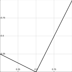
(a) Theorem 10

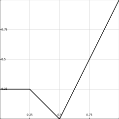
(b) Proposition 2

Figure 6. The graph of the function $g$ from the proof of Theorem 10 (left), and the function $g_{a}$ from the proof of Proposition 2, with $a=1/4$.

We now complete the proof of Theorem 3. Recall that the first half of the theorem, concerning the terminal nature of nonescaping and accessible points, was established in Theorems 8 and 10. Also recall that the set of nonescaping points in a given Julia continuum has Hausdorff dimension zero by Proposition 9. Hence it remains to prove that there is a disjoint-type entire function $f$ having a Julia continuum $\hat{C}$ such that the set of nonescaping points in $\hat{C}$ is a Cantor set, and another function having a Julia continuum containing a dense set of nonescaping points. Both results will be proved using Proposition 2.

To prove the second statement, we shall use the following general topological fact.

1 Proposition.

Let $X$ be an arc-like continuum. Suppose that $x$ is a terminal point of $X$, and that $E$ is a finite or countable set of terminal points, such that $X$ is irreducible between each of these points and $x$.

Then there is a sequence $g_{j}\colon[0,1]\to[0,1]$ of continuous and surjective functions such that $Y\mathrel{\vbox{\hbox{\scriptsize.}\hbox{\scriptsize.}}}=\varprojlim(g_{j})$ is homeomorphic to $X$, in such a way that $x$ corresponds to the point $1\mapsfrom 1\mapsfrom\dots$ and such that every point of $E$ corresponds to a point $x_{0}\mapsfrom x_{1}\mapsfrom\dots$ with $x_{j}=0$ for infinitely many $j$.

11.2 Proof.

This follows from the proof of [Nad92, Theorem 12.19], similarly as in the proof of Proposition 2. We omit the details.

To construct a Cantor set of nonescaping points, we make an explicit inverse limit construction.

2 Proposition (Cantor sets in inverse limit spaces).

There exists a sequence $(g_{n})_{n\geq 1}$ of surjective continuous maps $g_{n}\colon[0,1]\to[0,1]$, each fixing $1$, such that the inverse limit $Y\mathrel{\vbox{\hbox{\scriptsize.}\hbox{\scriptsize.}}}=\varprojlim(g_{n})$ has the following properties.

1. The set $A\mathrel{\vbox{\hbox{\scriptsize.}\hbox{\scriptsize.}}}=\{(x_{n})\in Y\colon x_{n}=0\text{ for infinitely many $n$}\}$ is a Cantor set;

2. every $(x_{n})\in Y\setminus A$ satisfies $\liminf_{n\to\infty}x_{n}>0$.

11.3 Proof.

For $a\in[0,1)$, let us define

$$g_{a}\colon[0,1]\to[0,1];\qquad x\mapsto\begin{cases}a&\text{if }x\leq\frac{1}{4}\\ a\cdot(2-4x)&\text{if }\frac{1}{4}<x\leq\frac{1}{2}\\ 2x-1&\text{if }\frac{1}{2}<x\leq 1.\end{cases}.$$

Note that $g_{a}(1-2^{-j})=g_{a}(1-2^{-(j-1)})$ for $j\geq 1$. The desired sequence of maps is given by $g_{n}\mathrel{\vbox{\hbox{\scriptsize.}\hbox{\scriptsize.}}}=g_{a_{n}}$, where $a_{1}=0$ and

(11.2) $$a_{n}\mathrel{\vbox{\hbox{\scriptsize.}\hbox{\scriptsize.}}}=1-\frac{1}{2^{\left\lfloor\frac{n-1}{2}\right\rfloor}}\quad(n\geq 2).$$

For $n\geq 2$, set

$$k(n)\mathrel{\vbox{\hbox{\scriptsize.}\hbox{\scriptsize.}}}=n-1-\lfloor(n-1)/2\rfloor=\lceil(n-1)/2\rceil=\lfloor n/2\rfloor.$$

By (11.2), if $k(n)\leq\tilde{k}<n$, then

$$g_{n,\dots,\tilde{k}}(0)=g_{(n-1),\dots,\tilde{k}}(a_{n})=1-2^{k(n)-\tilde{k}}.$$

In particular, $g_{n,\dots,k(n)}(0)=0$ and $g_{n,\dots,\tilde{k}}(0)\neq 0$ for $k<\tilde{k}<n$.

Now consider $Y=\varprojlim(g_{n})$ and the set $A$ from the statement of the proposition. Let $(x_{n})\in A$ and $k\geq 1$, and let $j$ be minimal with $x_{j}=0$ and $j\geq 2^{k}$. Then, by construction, $x_{k(j)}=x_{\lfloor j/2\rfloor}=0$, and hence $j<2^{k+1}$. So

$$A=\bigcap_{k\geq 1}\bigcup_{j=2^{k}}^{2^{k+1}-1}\{(x_{n})_{n\geq 0}\in Y\colon x_{j}=0\},$$

and $A$ is compact as an intersection of compact sets. Furthermore, $A$ is totally disconnected, as its projection to the $k$-th coordinate is countable for all $k$.

Fix $(x_{n})\in A$, and let $n_{0}\geq 1$ such that $x_{n_{0}}=0$. There are exactly two values of $n$ with $k(n)=n_{0}$, and hence $A$ contains at least one other point $(y_{n})$ with $y_{n_{0}}=0$. The distance between $(x_{n})$ and $(y_{n})$ tends to zero as $n_{0}\to\infty$, so $(x_{n})$ is not an isolated point. Thus we have proved that $A$ is a Cantor set, establishing a.

Finally, suppose that $(x_{n})\in Y$ and $\liminf_{n\to\infty}x_{n}=0$. Then there are infinitely many values of $n$ for which $x_{n}<1/4$, and hence $x_{n-1}=g_{n}(x_{n})=a_{n}=g_{n}(0)$. So

$$x_{k(n)}=g_{n,\dots,k(n)}(x_{n})=g_{n,\dots,k(n)}(0)=0.$$

Since $k(n)\to\infty$ as $n\to\infty$, we see that $(x_{n})\in A$, establishing claim b.

3 Corollary.

There exists a disjoint-type entire function $f$ having a Julia continuum $\hat{C}$ such that the set of nonescaping points is dense in $\hat{C}$.

There also exists a disjoint-type entire function $f$ having a Julia continuum $\hat{C}$ such that the set of nonescaping points in $\hat{C}$ is a Cantor set.

11.4 Remark.

This completes the proof of Theorem 3

11.5 Proof.

Let $Y$ be an arc-like continuum containing a terminal point $x$ and a dense countable set $E$ of terminal points such that $Y$ is irreducible between $x$ and $e$ for all $e\in E$. Apply Proposition 1 to obtain an inverse limit representation of $Y$ where the set $E$ consists of points having infinitely many components equal to $0$. By Proposition 2, there is a disjoint-type $F\in\mathcal{B}_{\log}^{\operatorname{p}}$ having a Julia continuum homeomorphic to $Y$, and such that every point of $E$ corresponds to a nonescaping point of $F$. An application of Theorem 5 now yields the first claim.

(An example of a continuum $Y$ with the desired property is given by the pseudo-arc. Indeed, since every point is terminal, we can simply select a countably dense subset $E$ of one composant, and choose $x$ in some other composant. We remark that it is also straightforward to construct such an inverse limit $Y$ with the desired properties directly, without using Proposition 1.)

The second claim follows in analogous manner, using the inverse limit from Proposition 2.

11.6 Remark.

A continuum containing a dense set of terminal points must necessarily be either indecomposable or the union of two indecomposable continua [CM87].

12. Realizing all arc-like continua by a single function

In this section, we complete the proof of Theorems 3, by showing that all the arc-like continua in question can be realised by a single function.

1 Theorem (A universal Julia set for arc-like continua).

There exists a disjoint-type function $F\in\mathcal{B}_{\log}^{\operatorname{p}}$ with the following property.

Let $Y$ be an arc-like continuum having a terminal point $y_{1}$, Then there is a Julia continum $\hat{J}_{\underline{s}}(F)$ such that $\hat{J}_{\underline{s}}(F)$ is homeomorphic to $Y$, with $\infty$ corresponding to $y_{1}$.

12.1 Proof.

By Proposition 3, there is a countable set $\mathcal{G}$ of functions $g\colon[0,1]\to[0,1]$ with $g(1)=1$ such that every arc-like continuum with a terminal point can be written as an inverse limit with bonding maps in $\mathcal{G}$.

Let $(S^{k})_{k\geq 1}$ be an enumeration of all finite sequences of maps in $\mathcal{G}$; that is, $k\mapsto S^{k}$ gives a bijection from $\mathbb{N}$ to the set of all finite sequences of maps in $\mathcal{G}$. Let us write $S^{k}=(g^{k}_{0},g^{k}_{1},\dots,g^{k}_{\ell_{k}})$, with $g^{k}_{j}\in\mathcal{G}$, for $k\geq 1$, and also let us write $\kappa$ for the inverse of this bijection; that is, $\kappa(S^{k})=k$. We may assume that no sequence $S$ appears before any of its prefixes in the enumeration. In other words, denote by $\sigma(S)$ the sequence obtained from $S$ by forgetting the final entry. Then $\kappa(\sigma(S))<\kappa(S)$. Here we use the convention that $\kappa(\sigma(S))=0$ if $S$ has length $1$.

We now set $g_{k}\mathrel{\vbox{\hbox{\scriptsize.}\hbox{\scriptsize.}}}=g^{k}_{\ell_{k}}$,

(12.1) $$k_{*}\mathrel{\vbox{\hbox{\scriptsize.}\hbox{\scriptsize.}}}=\kappa(\sigma(S^{k}))$$

and $M_{k}\mathrel{\vbox{\hbox{\scriptsize.}\hbox{\scriptsize.}}}=10$ for all $k$. We then carry out exactly the same construction as in the proof of Theorem 1, but using the above definition of $k_{*}$ instead of that in (10.5), and defining $n_{k}$ inductively by $n_{0}\mathrel{\vbox{\hbox{\scriptsize.}\hbox{\scriptsize.}}}=0$ and

$$n_{k}\mathrel{\vbox{\hbox{\scriptsize.}\hbox{\scriptsize.}}}=n_{k_{*}}+N_{k}+1,$$

instead of using (10.3). This yields a tract $T$, a function $F$ (and the associated map $\tilde{F}\in\mathcal{B}_{\log}^{\operatorname{p}}$), and sequences $N_{k}$ and $s(k)$ of integers.

If $S$ is an infinite sequence in $\mathcal{G}$, let $S(j)$ be the finite sequence consisting of the first $j$ entries of $S$, and set $k_{j}\mathrel{\vbox{\hbox{\scriptsize.}\hbox{\scriptsize.}}}=\kappa(S(j))$. Then $S=(g_{k_{j}})_{j\geq 1}$, and $k_{j}=(k_{j+1})_{*}$ for all $j$. Define an external address of $\tilde{F}$ by

$$\underline{s}\mathrel{\vbox{\hbox{\scriptsize.}\hbox{\scriptsize.}}}=\underline{s}(S)\mathrel{\vbox{\hbox{\scriptsize.}\hbox{\scriptsize.}}}=0^{N_{k_{1}}}s(k_{1})0^{N_{k_{2}}}s(k_{2})\dots.$$

The proof of Theorem 1 now goes through as before, with a small number of obvious adjustments to notation in the proofs of Proposition 9 and Theorem 1. For example, we should replace (10.10) by

(12.2) $$z_{j_{*}}\mathrel{\vbox{\hbox{\scriptsize.}\hbox{\scriptsize.}}}=f_{j}(z_{j})\qquad\text{and}\qquad x_{j_{*}}\mathrel{\vbox{\hbox{\scriptsize.}\hbox{\scriptsize.}}}=F^{-(N_{j}+1)}(x_{j}).$$

We conclude that $\hat{J}_{\underline{s}}(\tilde{F})$ is homeomorphic to $\varprojlim(g_{k_{j}})_{j=1}^{\infty}$. As every Julia continuum with a terminal point arises in this way, the proof is complete.

12.2 Proof (Proof of Theorem 3).

The first part of the theorem was established in Theorem 7 and Proposition 6. The second part of the theorem follows from Theorem 1, again combined with Theorem 5 to realise the example by a disjoint-type entire function.

13. Bounded-address Julia continua

We now turn our attention to constructing Julia continua at bounded external addresses with prescribed topology.

1 Theorem (Prescribed bounded-address Julia continua).

Let $Y$ be an arc-like continuum containing two terminal points $y_{0}$ and $y_{1}$ such that $Y$ is irreducible between $y_{0}$ and $y_{1}$. Then there exists a disjoint-type function $F\in\mathcal{B}_{\log}^{\operatorname{p}}$, having bounded slope and bounded decorations, and a bounded external address of $F$ such that the Julia continuum $\hat{J}_{\underline{s}}(F)$ is homeomorphic to $Y$. Under this homeomorphism, the unique point in $\hat{J}_{\underline{s}}(F)$ that has a bounded orbit corresponds to $y_{0}$, while $\infty$ corresponds to $y_{1}$.

The construction is very similar to the proof of Theorem 1. In order to construct a bounded address, we cannot, however, use “side channels” of a single tract as in Section 10. Hence we instead construct a function having exactly two tracts $S$ and $T$ modulo $2\pi i\mathbb{Z}$. Corollary 3 shows that this is indeed necessary.

Recall from Proposition 2 that $Y$ can be described as an inverse limit of functions $g_{k}\colon[0,1]\to[0,1]$ with $g_{k}(0)=0$ and $g_{k}(1)=1$. We fix this sequence for the remainder of the construction.

Description of the tracts $S$ and $T$

Both tracts are contained in the half-strip $\{x+iy\colon x>2\text{ and }-\pi/2<y<3\pi/2\}$. Similarly as in Section 10, we shall not require that the tracts are Jordan domains, or that their closures are disjoint. Once the conformal isomorphisms $F_{S}\colon S\to\mathbb{H}$ and $F_{T}\colon T\to\mathbb{H}$ are defined, we obtain a disjoint-type function $\tilde{F}$ by restriction and periodic extension as in Remark 3.

Figure 7. The tracts $S$ and $T$.

The first of the two tracts is the half-strip

$$S\mathrel{\vbox{\hbox{\scriptsize.}\hbox{\scriptsize.}}}=\{x+iy\colon x>2\text{ and }|y|<\pi/2\},$$

together with the function $F_{S}\colon S\to\mathbb{H}$ with $F_{S}(3)=3$ and $F_{S}^{\prime}(3)>0$. This tract plays essentially the same role as the central strip of the tract from Section 10: it is used to shift our Julia continuum sufficiently to the right.

The second tract,

$$T\subset\{x+iy\colon x>2\text{ and }\pi/2<y<3\pi/2\}$$

is determined by numbers $R_{k}^{-}$, $R_{k}^{+}$ with $4\leq R_{k}^{-}<R_{k}^{+}<R_{k+1}^{-}$, domains

$$U_{k}\subset\{x+iy\colon R_{k}^{-}<x<R_{k}^{+}\text{ and }\pi/2<y<3\pi/2\}$$

and arcs $C_{k}^{-}$ and $C_{k}^{+}$, with

$$C_{k}^{\pm}\subset\partial U_{k}\cap\{x+iy\colon x=R_{k}^{\pm}\}.$$

(See Figure 7.) The tract $T$ is defined as

$$T\mathrel{\vbox{\hbox{\scriptsize.}\hbox{\scriptsize.}}}=\bigcup_{k\geq 1}\{x+iy\colon R_{k-1}^{+}<x<R_{k}^{-}\text{ and }\pi/2<y<3\pi/2\}\cup\operatorname{int}(C_{k}^{-})\cup U_{k}\cup\operatorname{int}(C_{k}^{+}).$$

(Here we use the convention that $R_{0}^{+}=2$.) The function $F_{T}\colon T\to\mathbb{H}$ is chosen such that $F_{T}(3+\pi i)=3$ and $F_{T}(\infty)=\infty$.

The choices of $R_{k}^{\pm}$, $U_{k}$ and $C_{k}^{\pm}$ will again be specified in a recursive construction. For this purpose we define partial tracts

$$T_{k}\mathrel{\vbox{\hbox{\scriptsize.}\hbox{\scriptsize.}}}= \left(\bigcup_{j=1}^{k}\{x+iy\colon R_{j-1}^{+}<x<R_{j}^{-}\text{ and }\pi/2<y<3\pi/2\}\cup\operatorname{int}(C_{j}^{-})\cup U_{j}\cup\operatorname{int}(C_{j}^{+})\right)$$

$$\cup\{x+iy\colon x>R_{k}^{+}\text{ and }\pi/2<y<3\pi/2\},$$

and associated conformal isomorphisms $F_{k}\colon T_{k}\to\mathbb{H}$.

The external address in question is of the form

(13.1) $$\underline{s}=S^{N_{1}}TS^{N_{2}}TS^{N_{3}}T\dots.$$

We set $n_{k}\mathrel{\vbox{\hbox{\scriptsize.}\hbox{\scriptsize.}}}=k+\sum_{j\leq k}N_{j}$. The construction is very similar to the proof of Theorem 1. We construct the tract $T$ recursively along with a pseudo-conjugacy $(\psi_{k})$ between the system $(f_{k})$ defined by

$$f_{k}\colon\hat{S}\to\hat{S};\qquad z\mapsto F_{S}^{-N_{k}}(F_{T}^{-1}(z)),$$

where $\hat{S}=\overline{S}\cup\{\infty\}$, and the system $(g_{k})$. The maps $\psi_{k}$ are again of the form $\psi_{k}(z)=\varphi_{k}(\operatorname{Re}z)$, where $\varphi_{k}\colon[0,\infty]\to[0,1]$ is a homeomorphism on a certain interval $[M_{k},\widetilde{M}_{k}]$, and constant for $x\leq M_{k}$ and for $x\geq\widetilde{M}_{k}$. Note that $M_{k}\geq 4$ is no longer arbitrary as in Proposition 2, but instead determined as part of the construction.

The metric $d_{X_{k}}$ on $X_{k}=\hat{S}$ is defined as in (10.9), and the metric on $Y_{k}=[0,1]$ is once more the Euclidean metric, scaled up by a factor of $\gamma_{k}\in Y_{k}$.

The recursive construction is very similar to that in Section 10, so we focus on discussing those places where adjustments are needed; see also Figure 8. We define $\Xi_{k}$ and $(\xi^{j}_{k})$ as in Section 10, and again construct a finite set $\Omega_{k}\subset[0,1]$ as part of the construction. Begin by setting $M_{0}\mathrel{\vbox{\hbox{\scriptsize.}\hbox{\scriptsize.}}}=4$, $\widetilde{M}_{0}\mathrel{\vbox{\hbox{\scriptsize.}\hbox{\scriptsize.}}}=5$, $\varphi_{0}(x)=x-4$ for $4\leq x\leq 5$ and satisfying (10.4) elsewhere, and $\gamma_{0}\mathrel{\vbox{\hbox{\scriptsize.}\hbox{\scriptsize.}}}=5$. The number $k_{*}$ is used in exactly the same way as in Section 10. That is, $k_{*}=k-1$ for the purpose of the proof of Theorem 1, but a different choice is used in the proof of Theorem 5.

Figure 8. Construction of the tracts for Theorem 5.

I1. Step I1 is the same as in Section 10.

I2. Step I2 changes slightly, and indeed simplifies. The numbers $R_{k}^{-}$ and $R_{k}^{+}$ will be determined once $N_{k}$ is fixed, via

(13.2) $$R_{k}^{-}\mathrel{\vbox{\hbox{\scriptsize.}\hbox{\scriptsize.}}}=F_{S}^{N_{k}}(4)\qquad\text{and}\qquad R_{k}^{+}\mathrel{\vbox{\hbox{\scriptsize.}\hbox{\scriptsize.}}}=F_{S}^{N_{k}}(\widetilde{M}_{k_{*}}).$$

We then choose $N_{k}$ to satisfy (I2.3). Additionally, by choosing $N_{k}$ and hence $R_{k}^{-}$ sufficiently large, we can ensure – analogously to Observation 4 – that

(13.3) $$|F_{T}^{-1}(z)-F_{k-1}^{-1}(z)|\leq 1/k$$

when $|\operatorname{Im}z|\leq 2\pi$ and $1\leq\operatorname{Re}z\leq\widetilde{M}_{k-1}$.

I3. We set

$$\vartheta_{k}^{\ell}\mathrel{\vbox{\hbox{\scriptsize.}\hbox{\scriptsize.}}}=F_{S}^{N_{k}}(\varphi_{k_{*}}^{-1}(\xi_{k_{*}}^{\ell}))$$

for $0\leq\ell\leq\gamma_{k_{*}}$. The domains $U_{k}^{j}$ and arcs $C_{k}^{j}$, which together form the domain $U_{k}$, are chosen similarly as in Section 10; see Figure 8. The only changes from the conditions given in step I3 theere are that $\tilde{I}_{k}^{0}$ is extended to $R_{k}^{-}-1$ on the left, $\tilde{I}_{k}^{m_{k}}$ is extended to $R_{k}^{+}+1$ on the right, and (I3.2) becomes

(13.4) $$C_{k}^{-}\mathrel{\vbox{\hbox{\scriptsize.}\hbox{\scriptsize.}}}=C_{k}^{0}\subset\{x+iy\colon x=R_{k}^{-}\}\qquad\text{and}\qquad C_{k}^{+}\mathrel{\vbox{\hbox{\scriptsize.}\hbox{\scriptsize.}}}=C_{k}^{m_{k}}\subset\{x+iy\colon x=R_{k}^{+}\}.$$

This completes the description of the partial tract $T_{k}$ and the map $F_{k}$.

I4. There is no analogue of step I4. Observe that the curve $F_{k}^{-1}([2,\infty))$ is guaranteed to run through the entire domain $U_{k}$ by construction.

I5. Define

(13.5) $$M_{k} \mathrel{\vbox{\hbox{\scriptsize.}\hbox{\scriptsize.}}}=\min\{x\colon F_{k}^{-1}(x)\in C_{k}^{0}\}\qquad\text{and}$$

(13.6) $$\eta_{k}^{j} \mathrel{\vbox{\hbox{\scriptsize.}\hbox{\scriptsize.}}}=\max\{x\colon F_{k}^{-1}(x)\in C_{k}^{j}\}\qquad(j=1,\dots,m_{k}).$$

Then choose $\tilde{M}_{k}$ sufficiently large to ensure that

(13.7) $$F_{k}^{-1}(\tilde{M}_{k})>R_{k}^{+}+3\qquad\text{and}$$

(13.8) $$F_{S}^{-N_{1}}(F_{k}^{-1}(F_{S}^{-N_{2}}(F_{k}^{-1}(\dots(F_{S}^{-N_{k}}(F_{k}^{-1}(\tilde{M}_{k})))\dots))))\geq k.$$

Now $\varphi_{k}$ is defined as in (I5.3), and $\gamma_{k}$ is also chosen as in Section 10. This completes the inductive construction.

The analysis of the construction proceeds as in the proof of Theorem 1. We first establish the pseudo-conjugacy relation (10.6) in an analogous manner. (Observe that $R_{k}$ should be replaced by $R_{k}^{+}$ throughout, and that, for $j=1$, we should modify the definition of $\tilde{I}$ to $\tilde{I}\mathrel{\vbox{\hbox{\scriptsize.}\hbox{\scriptsize.}}}=\tilde{I}_{k}^{0}\cup[3,R_{k}^{-}]$.) The proof of Proposition 8 remains unchanged.

Finally, expansion of our system $(f_{k})$ follows from (13.2) and (I5.2), similarly as in Proposition 9. (Observe that the choice of $M_{k}$ in (13.5), together with that of $R_{k}^{-}$ in (13.2), ensure that the part of $S$ to the left of $M_{k}$ is mapped into a bounded set by $f_{k}$.) This completes the proof of Theorem 1.

13.1 Proof (Proof of Theorem 5).

In precisely the same manner as in Theorem 1, we can realise all the relevant continua as bounded-address Julia continua of the same function. Note that, in the construction, we should now replace (13.8) by

$$F_{S}^{-N_{k_{1}}}(F_{k}^{-1}(F_{S}^{-N_{k_{2}}}(F_{k}^{-1}(\dots(F_{S}^{-N_{k}}(F_{k}^{-1}(\tilde{M}_{k})))\dots))))\geq k,$$

where $k_{1}<k_{2}<\dots<k_{\ell}=k$ are chosen such that $k_{i}=(k_{i+1})_{*}$ and $(k_{1})_{*}=0$.

2 Remark (Alternative proof of Theorem 3).

We observe that, using Theorem 5, we can give an alternative proof of (the second half of) Theorem 3.

Indeed, let $X$ be any arc-like continuum having a terminal point $x_{1}$. Then there is an arc-like continuum $Y\supset X$ having a terminal point $x_{0}$ such that $Y$ is irreducible between $x_{0}$ and $x_{1}$. (Indeed, $X$ can be written as the inverse limit of a sequence of continuous surjective functions $g_{k}\colon[0,1]\to[0,1]$ with $g_{k}(1)=1$. We can extend each $\tilde{g}_{k}$ to a map $[-1,1]\to[-1,1]$ fixing $-1$, and the inverse limit of these extensions is the desired continuum $Y$.

Since the function $f$ from Theorem 5 has bounded slope, it follows from Theorem 4 that every arc-like continuum having a terminal point is also realised as a Julia continuum of $f$.

A key difference between the two proofs is that the Julia continua from Theorem 4 escape uniformly to infinity, so the examples in Section 11 cannot be obtained in this manner. Furthermore, the function constructed in our original proof has only one tract, but does not have bounded decorations, while the construction of Theorem 5 has bounded decorations, but also requires two tracts. Recall from Corollary 10 that it is impossible to achieve both at the same time.

14. Periodic Julia continua

We now construct periodic Julia continua, proving Theorem 7.

1 Theorem (Constructing invariant Julia continua).

Let $\hat{Y}$ be a continuum, and suppose that there are $y_{0},y_{1}\in\hat{Y}$ such that $\hat{Y}$ is a Rogers continuum from $y_{0}$ to $y_{1}$. There exist a logarithmic tract $T$ with $\overline{T}\subset\mathbb{H}$ and a conformal isomorphism $F\colon T\to\mathbb{H}$ with $F(\infty)=\infty$ such that

$$\hat{C}\mathrel{\vbox{\hbox{\scriptsize.}\hbox{\scriptsize.}}}=\{z\in T\colon F^{n}(z)\in T\text{ for all $n\geq 0$}\}\cup\{\infty\}$$

is homeomorphic to $\hat{Y}$, with $\infty$ corresponding to $y_{1}$, and the unique finite fixed point of $F$ corresponding to $y_{0}$.

Moreover, $T$ can be chosen to have bounded slope and bounded decorations.

Let us fix $\hat{Y}$ for the remainder of the section, and let $g\colon[0,1]\to[0,1]$ be as in the definition of Rogers continua. That is, $g$ fixes $0$ and $1$, $g(x)<x$ for $0<x<1$, and $\varprojlim([0,1],g)$ is homeomorphic to $\hat{Y}$. Let $(\tau_{k})_{k\geq 0}$ be a strictly increasing sequence in $(0,1)$ such that

1. $g(x)<g(\tau_{k})$ for all $x<\tau_{k}$ and

2. $g(\tau_{k+3})=\tau_{k}$

for all $k\geq 0$. For example, such a sequence can be defined by

$$\tau(a) \mathrel{\vbox{\hbox{\scriptsize.}\hbox{\scriptsize.}}}=\min\{\tau\in[0,1]\colon g(\tau)=a\}\quad(a\in[0,1]),$$

$$\tau_{0}\mathrel{\vbox{\hbox{\scriptsize.}\hbox{\scriptsize.}}}=\tau(1/2),\quad\tau_{1} \mathrel{\vbox{\hbox{\scriptsize.}\hbox{\scriptsize.}}}=\tau\left(\frac{1+\tau_{0}}{3}\right),\quad\tau_{2}\mathrel{\vbox{\hbox{\scriptsize.}\hbox{\scriptsize.}}}=\tau\left(\frac{1+4\tau_{0}}{6}\right)\quad\text{and}\quad\tau_{k+3}\mathrel{\vbox{\hbox{\scriptsize.}\hbox{\scriptsize.}}}=\tau(\tau_{k})\quad(k\geq 0).$$

This sequence has the desired properties since $\tau(a)>a$ for all $a\in(0,1)$ and since $\tau(a)$ is strictly increasing in $a$. Observe that $\tau_{k}\to 1$, as $1$ is the only positive fixed point of $g$. For convenience, we set $\tau_{k-3}\mathrel{\vbox{\hbox{\scriptsize.}\hbox{\scriptsize.}}}=g(\tau_{k})$ for $k=1,2$.

The fact that

(14.2) $$g(x)\leq g(\tau_{k})=\tau_{k-3}<\tau_{k-2},\qquad\tau_{k-1}\leq x\leq\tau_{k},\qquad k\geq 1,$$

allows us to construct the tract $T$ in stages, with the $k$-th piece representing

(14.3) $$g\colon A_{k}\to B_{k-3},\qquad\text{where}\quad A_{k}\mathrel{\vbox{\hbox{\scriptsize.}\hbox{\scriptsize.}}}=[\tau_{k-1},\tau_{k}],\quad B_{k-3}\mathrel{\vbox{\hbox{\scriptsize.}\hbox{\scriptsize.}}}=[0,\tau_{k-3}].$$

The same fact also allows us to express $g|_{[0,1)}$ as an expanding system, to which we will be able to apply Proposition 6. Indeed, let $(\gamma_{k})_{k\geq 0}$ be a sequence of numbers $\gamma_{k}\geq 1$. We define a metric $d_{Y}$ on $Y\mathrel{\vbox{\hbox{\scriptsize.}\hbox{\scriptsize.}}}=[0,1)$ as follows.

1. When restricted to $B_{0}$, $d_{Y}$ is some metric equivalent to the Euclidean metric, and the $d_{Y}$-length of $B_{0}$ is $\ell_{d_{Y}}(B_{0})=\gamma_{0}$.

2. For every $k\geq 1$, the metric $d_{Y}$ is a constant multiple of the Euclidean metric on $A_{k}$, and $\ell_{d_{Y}}(A_{k})=\gamma_{k}$.

2 Observation (Expanding metric for $g$).

There are functions $\Gamma_{k}\colon[1,\infty)\to[1,\infty)$ with the following property. If $\gamma_{k}\geq\Gamma_{k}(\gamma_{k-1})$ for all $k\geq 1$, then $g\colon Y\to Y$ is an expanding inverse system with respect to $d_{Y}$, with expansion constants $\lambda=2$ and $K=8\gamma_{0}$.

14.1 Proof.

Since $g^{k}(x)\to 0$ locally uniformly for $x\in[0,1)$, condition 2 of Definition 1 holds automatically for $g|_{B_{0}}\colon B_{0}\to B_{0}$.

As in Observation 3, it is easy to define $\Gamma_{k}$ such that condition 2 also holds on $A_{k}$, and such that $g|_{A_{k}}\colon A_{k}\to B_{k-3}$ satisfies (4.1), say for $\tilde{\lambda}=4$ and $\tilde{K}=1$, for all $k\geq 1$. (Observe that the definition of the metric on $B_{k-3}$ does not depend on that on $A_{k}$.)

Now suppose that a sequence $(\gamma_{k})$ with the stated properties is given, and let $x,y\in[0,1)$; we must establish (4.1) for $d_{Y}$ and $g$. Set $I_{0}\mathrel{\vbox{\hbox{\scriptsize.}\hbox{\scriptsize.}}}=[x,y]\cap B_{0}$ and $I_{k}\mathrel{\vbox{\hbox{\scriptsize.}\hbox{\scriptsize.}}}=[x,y]\cap A_{k}$ for $k\geq 1$. Let $\mathcal{K}$ be the set of $k\geq 0$ for which $I_{k}\neq\emptyset$; say $I_{k}=\{k_{0},\dots,k_{1}\}$, and let $\tilde{\mathcal{K}}\subset\mathcal{K}$ consist of those $k\geq 1$ for which the $d_{Y}$-length $\ell_{d_{Y}}(I_{k})\geq\tilde{K}=1$. If $k\in\mathcal{K}\setminus\tilde{\mathcal{K}}$, then either $k=0$ and $\ell_{d_{Y}}(g(I_{k}))\leq\gamma_{0}$, or $k\in\{k_{0},k_{1}\}$ and $\ell_{d_{Y}}(g(I_{k}))\leq 1/4<\gamma_{0}$ by (4.1). On the other hand, if $k\in\tilde{\mathcal{K}}$, then $\ell_{d_{Y}}(g(I_{k}))\leq\ell_{d_{Y}}(I_{k})/4$ by (4.1). Hence

$$d_{Y}(g(x),g(y))\leq\sum_{k\in\mathcal{K}}\ell_{d_{Y}}(g(I_{k})) \leq 2\gamma_{0}+\frac{1}{4}\sum_{k\in\tilde{\mathcal{K}}}\ell_{d_{Y}}(I_{k})\leq$$

$$2\gamma_{0}+\frac{1}{4}\sum_{k\in\mathcal{K}}\ell_{d_{Y}}(I_{k}) =2\gamma_{0}+\frac{1}{4}d_{Y}(x,y)\leq\frac{\max(8\gamma_{0},d_{Y}(x,y))}{2}.$$

Figure 9. The shape of the tract $T$ used to construct a prescribed invariant Julia continuum.

Description of $F$ and $T$

Our tract $T$ is given as a disjoint union of the form

$$T=\bigcup_{j\geq 0}U_{j}\cup\operatorname{int}(C_{j})\subset\{x+iy\colon x>4,|y|<\pi\}.$$

(See Figure 9.) Here $(C_{j})_{j\geq 0}$ is a sequence of cross-cuts of $T$, with $C_{j-1}$ and $C_{j}$ bounding the subdomain $U_{j}$ in $T$ for $j\geq 1$. Furthermore,

$$U_{0} =\{x+iy\colon 4<x<R_{0},|y|<\pi/2\},$$

(14.5) $$U_{j} \subset\left\{x+iy\colon 4<x<R_{j},-\pi/2\cdot\left(1+\frac{j}{j+1}\right)<y<\pi/2\right\}\quad(j\geq 1),\quad\text{and}$$

$$C_{j} \subset\{R_{j}+iy\colon|y|\leq\pi\}\cap\partial U_{j}\cap\partial U_{j+1},$$

where $(R_{k})$ is a strictly (and rapidly) increasing sequence of numbers $R_{k}\geq 10$, and the domains $U_{j}$ converge uniformly to $\infty$ as $j\to\infty$.

The conformal isomorphism $F\colon T\to\mathbb{H}$ is uniquely determined by requiring $F(5)=5$ and $F(\infty)=\infty$. We also define partial tracts

$$T_{k}\mathrel{\vbox{\hbox{\scriptsize.}\hbox{\scriptsize.}}}=\bigcup_{j=0}^{k}U_{j}\cup\bigcup_{j=0}^{k-1}\operatorname{int}(C_{j})$$

(observe that $T_{k}$ is bounded). The associated conformal isomorphisms $F_{k}\colon T_{k}\to\mathbb{H}$ is determined by requiring $F_{k}(5)=5$ and $F_{k}(\xi_{k})=\infty$, where $\xi_{k}\in C_{k}$ is defined as part of the construction. In analogy with Observation 4, we have the following.

3 Observation (Approximation by partial tracts).

Let $k\geq 0$. Suppose that $(U_{j})$ has been chosen for $j\leq k$, that $C_{j}$ has been chosen for $j<k$, and that $\zeta_{k}\in\partial U_{k}$ has been chosen with $\operatorname{Re}\zeta_{k}=R_{k}$, so that $T_{k}$ and $F_{k}$ are defined. Let $R>0$.

Then there is an arc $\tilde{C}_{k}\subset\partial U_{k}$ with $\zeta_{k}\in\tilde{C}_{k}$ with the following property. Suppose that the remaining choices of $U_{j}$ and $C_{j}$ are made such that $C_{k}\subset\tilde{C}_{k}$, and otherwise only subject to the conditions above. Then

$$\operatorname{dist}_{T_{k}}(F_{k}^{-1}(x),F_{\ell}^{-1}(x))\leq\frac{1}{4}$$

for $k+1\leq\ell\leq\infty$ and $4\leq x\leq R$. (Here we use the convention that $F_{\infty}=F$.)

Recursive construction

The definition of the domains $U_{k}$ and arcs $C_{k}$ is carried out in a similar spirit to those in Sections 10 and 13. As part of the construction, we obtain a homeomorphism

$$\varphi\colon[4,\infty)\to[0,1),$$

where

$$\varphi|_{[R_{k+2},R_{k+3}]}\colon[R_{k+2},R_{k+3}]\to A_{k}$$

is defined in the $(k+2)$-th step of the construction. $\varphi$ will satisfy $\varphi(R_{k})=\tau_{k-3}$ for all $k\geq 1$. The construction ensures that

(14.6) $$\psi\colon\overline{T}\to[0,1);\qquad\psi(z)\mathrel{\vbox{\hbox{\scriptsize.}\hbox{\scriptsize.}}}=\varphi(\operatorname{Re}z)$$

is a pseudo-conjugacy between the systems $(\overline{T},F^{-1})$, with the Euclidean metric, and $([0,1),g)$, with the metric $d_{Y}$ defined above, with $(\gamma_{k})$ chosen recursively during the construction.

The $\gamma_{k}$ are chosen to be a natural numbers. The metric on $B_{0}$ will be chosen to be a linear multiple of the Euclidean metric on each of the intervals $B_{-2}=[0,\tau_{-2}]$, $[\tau_{-2},\tau_{-1}]$ and $[\tau_{-1},\tau_{0}]$, with each interval having integer length. The choice of $d_{Y}$ on $B_{k}$ determines a finite set

$$\Xi_{k}\mathrel{\vbox{\hbox{\scriptsize.}\hbox{\scriptsize.}}}=\{\xi\in B_{k}\colon d_{Y}(0,\xi)\in\mathbb{Z}\}\supset\{0,\tau_{-2},\dots,\tau_{k}\}$$

that partitions $B_{k}$ into intervals of unit $d_{Y}$-length.

To anchor the recursion, set

$$R_{-1}\mathrel{\vbox{\hbox{\scriptsize.}\hbox{\scriptsize.}}}=10,\quad R_{0}\mathrel{\vbox{\hbox{\scriptsize.}\hbox{\scriptsize.}}}=14\quad\text{and}\quad R_{1}\mathrel{\vbox{\hbox{\scriptsize.}\hbox{\scriptsize.}}}=15.$$

We define $\varphi\colon[4,R_{1}]\to[0,\tau_{-2}]$ to be linear with $\varphi(4)=0$ and $\varphi(R_{1})=\tau_{-2}$, and define the metric $d_{Y}$ on $[0,\tau_{-2}]$ by

(14.7) $$d_{Y}(x,y)\mathrel{\vbox{\hbox{\scriptsize.}\hbox{\scriptsize.}}}=5|\varphi^{-1}(x)-\varphi^{-1}(y)|.$$

We also set $\zeta_{0}\mathrel{\vbox{\hbox{\scriptsize.}\hbox{\scriptsize.}}}=R_{0}$.

Now the inductive step proceeds as follows. Let $k\geq 1$. Assume that the domains $U_{i}$ are chosen for $i<k$, and the arcs $C_{i}$ for $i<k-1$. The point $\zeta_{k-1}$ will also have been chosen, so $F_{k-1}$ is defined. Moreover, $R_{i}$ is defined for $i\leq k$, an order-preserving homeomorphism $\varphi\colon[4,R_{k}]\to[0,\tau_{k-3}]$ has been constructed, and the metric $d_{Y}$ has been defined on $B_{k-3}$. A finite set

$$\Omega_{i}=\{\tau_{i-1}=\omega_{i}^{0}<\omega_{i}^{1}<\dots<\omega_{i}^{m_{i}}=\tau_{i}\}$$

will also have been chosen for $i<k$.

As in (I3.2), each domain $U_{i}$ (for $1\leq i<k$) is given by a finite union

$$U_{i}=\bigcup_{j=1}^{m_{i}}U_{i}^{j}\cup\bigcup_{j=1}^{m_{i}-1}C_{i}^{j}$$

of quadrilaterals $U_{i}^{j}$ and arcs $C_{i}^{j}$ connecting them, together with arcs $C_{i}^{0}=C_{i-1}$ and $C_{i}^{m_{i}}\supset C_{i}$. To avoid special consideration of special cases in the case of $k=1,2$, we also define $m_{1}\mathrel{\vbox{\hbox{\scriptsize.}\hbox{\scriptsize.}}}=m_{0}\mathrel{\vbox{\hbox{\scriptsize.}\hbox{\scriptsize.}}}=1$, and set

$$U_{-1}^{1} \mathrel{\vbox{\hbox{\scriptsize.}\hbox{\scriptsize.}}}=\{x+iy\colon 5<x<R_{-1},|y|<\pi/2\},$$

$$U_{0}^{1} \mathrel{\vbox{\hbox{\scriptsize.}\hbox{\scriptsize.}}}=\{x+iy\colon R_{-1}<x<R_{0},|y|<\pi/2\},$$

$$C_{-1}^{0} \mathrel{\vbox{\hbox{\scriptsize.}\hbox{\scriptsize.}}}=\{5+iy\colon|y|\leq\pi/2\},\quad C_{-1}^{1}\mathrel{\vbox{\hbox{\scriptsize.}\hbox{\scriptsize.}}}=C_{0}^{0}\mathrel{\vbox{\hbox{\scriptsize.}\hbox{\scriptsize.}}}=\{R_{-1}+iy\colon|y|\leq\pi/2\},\quad\text{and}\quad$$

$$C_{0}^{1} \mathrel{\vbox{\hbox{\scriptsize.}\hbox{\scriptsize.}}}=\{R_{0}+iy\colon|y|\leq\pi/2\}.$$

It turns out to be convenient to slightly change the order of steps compared with those in Section 10; more precisely, we shall begin the inductive step with the analogue of step I5. To emphasise the similarity with previous sections, we shall retain the same numbering.

I5. For $j=0,\dots,m_{k-2}$, define

(14.8) $$\eta_{k-2}^{j}\mathrel{\vbox{\hbox{\scriptsize.}\hbox{\scriptsize.}}}=\min\{x\in[5,\infty)\colon F_{k-1}^{-1}(x)\in C_{k-2}^{j}\}.$$

We set $R_{k+1}\mathrel{\vbox{\hbox{\scriptsize.}\hbox{\scriptsize.}}}=\eta_{k-2}^{m_{k-2}}$. We now extend $\varphi$ to $[R_{k},R_{k+1}]$ in a piecewise linear manner such that

$$\varphi(\eta_{k-2}^{j})=\omega_{k-2}^{j}$$

for $j=1,\dots,m_{k-1}$. We shall see in the proof of Theorem 1 below that

(14.9) $$\eta^{1}_{k-2}>R_{k}.$$

Hence this does indeed define a homeomorphism $[R_{k},R_{k+1}]\to[\tau_{k-3},\tau_{k-2}]$.

We now define the metric $d_{Y}$ on $I\mathrel{\vbox{\hbox{\scriptsize.}\hbox{\scriptsize.}}}=[\tau_{k-3},\tau_{k-2}]$ to be a constant multiple of the Euclidean metric, subject to the following requirements. Note that $I=A_{k-2}$ for $k\geq 3$.

1. $I$ has integer length;

2. if $\tilde{I}\subset I$ has $\ell_{d_{Y}}(\tilde{I})\leq 1$, then $\operatorname{diam}(\varphi^{-1}(\tilde{I}))<1/4$;

3. if $k\geq 3$, then $\gamma_{k-2}\mathrel{\vbox{\hbox{\scriptsize.}\hbox{\scriptsize.}}}=\ell_{Y}(I)\geq\Gamma_{k-2}(\gamma_{k-3})$. (Recall that $\Gamma_{k-2}$ was defined in Observation 2, and that $\gamma_{0}=\ell_{Y}(B_{0})$ by definition.)

I1. As in (I1.1), we choose $m_{k}$ and $\Omega_{k}$ such that, for $1\leq j\leq m_{k}$, the image $g([\omega_{k}^{j-1},\omega_{k}^{j}])$ contains at most one element of $\Xi_{k-3}\setminus\{0\}$.

I2. Choose an arc $\tilde{C}_{k-1}\subset C_{k-1}^{m_{k-1}}$ with $\zeta_{k-1}\in\operatorname{int}(\tilde{C}_{k-1})$ by applying Observation 3 to $T_{k-1}$. Here we use $R=R_{k+1}$.

I3. We now define the domain $U_{k}$, very similarly to step I3 in Section 10. For $j\in\{1,\dots,m_{k}\}$, let $I_{k}^{j}$ be the smallest closed interval bounded by two points of $\Xi_{k-2}$ whose interior contains $g([\omega_{k}^{j-1},\omega_{k}^{j}])\setminus\{0\}$. We also define $\tilde{I}_{k}^{j}\mathrel{\vbox{\hbox{\scriptsize.}\hbox{\scriptsize.}}}=\varphi^{-1}(I_{k}^{j})$. (Note that, in contrast to Section 10, there is no need for a different definition when $j=m_{k}$.)

Requirement (I3.1) remains unchanged from Section 10, as does (I3.3). Condition (I3.2) is replaced by

1. $C_{k-1}\mathrel{\vbox{\hbox{\scriptsize.}\hbox{\scriptsize.}}}=C_{k}^{0}\subset\tilde{C}_{k-1}$ and $C_{k}^{m_{k}}\subset\{R_{k}+iy\colon|y|\leq\pi\}$.

Requirements (I3.4) and (I3.5) are slightly changed as follows, for each $1\leq j\leq m_{k}$.

1. For $k\leq m\leq\infty$, $\operatorname{dist}_{T_{m}}(C_{k}^{j-1},C_{k}^{j})\geq 1$.

2. Let $k\leq m\leq\infty$, and suppose that $\alpha$ is a geodesic segment of $T_{m}$ that connects $C_{k}^{j-1}$ and $C_{k}^{j}$. Then $\operatorname{dist}_{T}(z,U_{k}^{j})\leq 1/4$ for all $z\in\alpha$. (I.e., $\alpha$ cannot protrude too far from the cross-cuts $C_{k}^{j-1}$ and $C_{k}^{j}$.)

(Here we again use the convention that $T_{\infty}=T$.) Finally, we require the following, to ensure the bounded decorations condition for the tract $T$.

1. All $U_{k}^{j}$ have bounded decorations (uniformly in $k$ and $j$). By this we mean the following: Every point of $U_{k}^{j}$ can be connected to both arcs of $\partial U_{k}^{j}\setminus(C_{k}^{j-1}\cup C_{k}^{j})$ by a curve whose diameter is uniformly bounded (say, by $2\pi$). (Here we are assuming for simplicity that $U_{k}^{j}$ is a Jordan domain, which can always be achieved. However, it is straightforward to extend this definition to non-Jordan domains with locally connected boundary.)

We also choose $\zeta_{k}\in\operatorname{int}(C_{k}^{m_{k}})$, completing the description of $T_{k}$ and $F_{k}$.

I4. There is no analogue of step I4, and the inductive construction is complete.

14.2 Proof (Proof of Theorem 1).

We first verify that the construction indeed guarantees (14.9). For $k=1$, this follows from the standard estimate (2.1). So suppose that $k\geq 2$, and let $4\leq x\leq R_{k}$. Then $F_{k-2}^{-1}(x)\in T_{k-3}$ by definition of $R_{k}$. Furthermore, $\operatorname{dist}_{T_{k-2}}(F_{k-1}^{-1}(x),F_{k-2}^{-1}(x))\leq 1/4$ by step I2. Hence, by (14.12), $F_{k-1}^{-1}(x)\not\in C_{k-2}^{1}$ for these values of $x$. In particular, $\eta^{1}_{k-2}>R_{k}$, as required.

Now let $T$ be the tract we have just defined. Then $T$ clearly has bounded slope. The tract also has bounded decorations by Proposition 4 and (14.13).

The (autonomous) inverse system generated by $(\overline{T},F^{-1})$ is expanding when equipped with the Euclidean metric (using an analogue of Observation 5). The system $([0,1),g)$ with the metric $d_{Y}$ is expanding by (14.12).

We claim that $\psi\colon\overline{T}\to[0,1)$ is a pseudo-conjugacy between the two systems. To establish the pseudo-conjugacy relation, let $w\in\overline{T}$; we claim that

(14.14) $$\operatorname{dist}_{Y}(g(\psi(w)),\psi(F^{-1}(w)))\leq\max(4,\gamma_{0}).$$

Set $\omega\mathrel{\vbox{\hbox{\scriptsize.}\hbox{\scriptsize.}}}=\psi(w)$, $x\mathrel{\vbox{\hbox{\scriptsize.}\hbox{\scriptsize.}}}=\operatorname{Re}w$ and $z\mathrel{\vbox{\hbox{\scriptsize.}\hbox{\scriptsize.}}}=F^{-1}(w)$. Set $k=0$ if $\omega\in B_{0}$, and otherwise let $k$ be such that $\omega\in A_{k}$. Then $x\leq R_{k+3}$, and hence

(14.15) $$\operatorname{dist}_{T}(F_{k+1}^{-1}(x),F^{-1}(x))\leq\operatorname{dist}_{T_{k+1}}(F_{k+1}^{-1}(x),F^{-1}(x))\leq 1/4$$

by I2. Since $F\colon T\to\mathbb{H}$ is a conformal isomorphism, also

(14.16) $$\operatorname{dist}_{T}(z,F^{-1}(x))\leq\pi/x.$$

First suppose that $k=0$. Then $g(\psi(w))\in B_{0}$ and $x\leq R_{3}$. Thus $F_{1}^{-1}(x)\in U_{0}$ by definition, and $F^{-1}(w)\in T_{2}$ by (14.15) and (14.16). So $\psi(z)\in B_{0}$, and (14.14) follows.

Now suppose that $k\geq 1$ and $x>\eta_{k}^{0}$, as defined in (14.8). Let $j\in\{1,\dots,m_{k-1}\}$ be such that $\eta_{k}^{j-1}<x\leq\eta_{k}^{j}$. Then $F_{k+1}^{-1}(x)$ belongs to a geodesic segment of $T_{k}$ connecting $C_{k}^{j-1}$ and $C_{k}^{j}$, and hence by (14.13),

$$\operatorname{dist}_{T}(F_{k+1}^{-1}(x),U_{k}^{j})\leq 1/4.$$

Note that $x\geq R_{0}\geq 10$, and hence (14.15) and (14.16), together with (14.12), imply that $z$ either belongs to $U^{j}_{k}$, or to one of the quadrilaterals adjacent to $U^{j}_{k}$. Recall that $g(\omega)\in\tilde{I}^{j}_{k}$, which has $d_{Y}$-length at most $2$. It follows that $d_{Y}(g(\omega),\psi(z))\leq 3$, as desired.

Finally, suppose that $R_{k+2}\leq x\leq\eta_{k}^{0}$. For $5\leq\zeta\leq\eta_{k}^{0}$, we have $F_{k+1}^{-1}(\zeta)\in T_{k-1}$ by definition of $\eta_{k}^{0}$. Moreover, $\operatorname{dist}_{T_{k}}(F_{k}^{-1}(R_{k+2}),F_{k+1}^{-1}(R_{k+2}))\leq 1/4$ by step I2, and hence $F_{k+1}^{-1}(R_{k+2})\in U_{k-1}^{m_{k-1}}$.

So if $\rho\in[5,\infty)$ is minimal with $F_{k+1}^{-1}(\rho)\in C_{k-1}^{m_{k-1}-1}$, then $\rho\leq R_{k+2}\leq x$. Thus $x$ belongs to a geodesic of $T_{k+1}$ connecting the two cross-cuts bounding $U_{k-1}^{m_{k-1}}$. By (14.13), we have $\operatorname{dist}_{T}(x,U_{k-1}^{m_{k-1}})\leq 1/4$. Arguing as above, we conclude that $d_{Y}(g(\omega),\psi(z))\leq 4$, and the proof of (14.14) is complete.

Surjectivity of $\psi$ is obvious, and the remaining two conditions follow as in Proposition 8. So the two inverse limits are homeomorphic, and the homeomorphism extends to their one-point compactifications, $\hat{C}$ and $\hat{Y}$, with $\infty$ corresponding to $y_{1}$. Moreover, by Observation 7, the unique fixed point of $F$ in $C$ must correspond to $y_{0}$. This completes the proof.

14.3 Proof (Proof of Theorem 7).

The fact that every invariant Julia continuum of a function with bounded-slope tracts is of the required form was already established in Theorem 7. Conversely, by Theorem 5, we can realise the invariant Julia continuum from Theorem 1 by a disjoint-type entire function of bounded slope.

14.4 Proof (Proof of Theorem 5).

By a classical result of Henderson [Hen64], the pseudo-arc can be written as an inverse limit of a single function $f\colon[0,1]\to[0,1]$ with $f(x)<x$ for all $x\in(0,1)$. By Theorem 1, there is a disjoint-type function $F\in\mathcal{B}_{\log}^{\operatorname{p}}$, having only one tract $T$, such that the invariant Julia continuum in $T$ is a pseudo-arc. Furthermore, this tract has bounded slope and bounded decorations, and hence Corollary 8 implies that every Julia continuum is a pseudo-arc.

Finally, by Theorem 5, there is a disjoint-type function $f\in\mathcal{B}$ with the same property.

15. Making examples with a finite number of tracts and singular values

We now turn to Theorem 11. So far, we have shown that each of the examples in question can be constructed in the class $\mathcal{B}$, with the desired number of tracts (one or two). With the exception of Theorem 5, in which we require control over all Julia continua, Theorem 5 also shows that they can be constructed in the class $\mathcal{S}$, but with a potentially infinite number of tracts.

In order to show that we can also realise our examples in the class $\mathcal{S}$, without having to add addional tracts, we need to use Bishop’s results from [Bis15a], rather than those from [Bis17]. Let $G$ be an infinite locally bounded tree in the plane. Following Bishop, we say that $G$ has bounded geometry if the following hold.

1. The edges of $G$ are $C^{2}$, with uniform bounds.

2. The angles between adjacent edges are bounded uniformly away from zero.

3. Adjacent edges have uniformly comparable lengths.

4. For non-adjacent edges $e$ and $f$, we have $\operatorname{diam}(e)\leq C\cdot\operatorname{dist}(e,f)$ for some constant $C$ depending only on $G$.

Bishop’s theorem [Bis15a, Theorem 1.1] is as follows:

1 Theorem (Construction of entire functions with two singular values).

Suppose that $G$ has bounded geometry. Suppose furthermore that $\tau\colon\mathbb{C}\setminus G\to\mathbb{H}$ is holomorphic with the following properties.

1. For every component $\Omega_{j}$ of $\mathbb{C}\setminus G$, $\tau\colon\Omega_{j}\to\mathbb{H}$ is a conformal isomorphism whose inverse $\sigma_{j}$ extends continuously to the closure of $\mathbb{H}$ with $\sigma_{j}(\infty)=\infty$.

2. For every (open) edge $e\in G$, and each $j$, every component of $\sigma_{j}^{-1}(e)\subset\partial\mathbb{H}$ has length at least $\pi$.

Then there is an entire function $f\in\mathcal{S}$ and a $K$-quasiconformal map $\varphi$ such that $f\circ\varphi=\cosh\circ\tau$ on the complement of the set

$$G(r_{0})\mathrel{\vbox{\hbox{\scriptsize.}\hbox{\scriptsize.}}}=\bigcup_{e\in G}\{z\in\mathbb{C}\colon\operatorname{dist}(z,e)<r_{0}\operatorname{diam}(e)\}.$$

(Here $r_{0}$ is a universal constant, and the union is over all edges of $G$.)

The only critical points of $f$ are $\pm 1$ and $f$ has no asymptotic values. If $d$ is such that $G$ has no vertices of valence greater than $d$, then $f$ has no critical points of degree greater than $4d$.

2 Remark (Smaller bounds on the degree).

This is the theorem as stated in [Bis17, Theorem 3.1]. All trees considered in this section will have maximal degree at most $4$, leading to a bound of $16$ on the degree of critical points. As discussed in [Bis17], the bound of $4d$ can be reduced to $\max(4,d)$ by modifying the construction in [Bis17], and replacing $\tau$ by an integer multiple. This leads to a bound of $4$ on the critical points of our functions, as remarked in Section 2.

In order to use this result to obtain the desired examples, there are two steps that we need to take.

• We will modify the construction of the domains $\mathcal{T}$ of our functions, to obtain a union $\tilde{\mathcal{T}}$ of “tracts” such that $\mathbb{C}\setminus\exp(\tilde{T})$ is a bounded-geometry tree.

  Along with these tracts, we construct $\tilde{F}\colon\tilde{\mathcal{T}}\to\mathbb{H}$, conformal on each component of $\tilde{\mathcal{T}}$, such that the map $\tau(\exp(z))\mathrel{\vbox{\hbox{\scriptsize.}\hbox{\scriptsize.}}}=\tilde{F}(z)$ satisfies the hypotheses of Theorem 1.

  When we consider the restriction $F$ of $\tilde{F}$ to the preimage of a suitable right half-plane, we will obtain a disjoint-type function in $\mathcal{B}_{\log}^{\operatorname{p}}$, still having the desired properties of the original construction.

  Observe that $\overline{\mathcal{T}}$ will need to fill out the entire plane, which means that we have to ensure that the individual tracts each fill out a complete horizontal strip of height $2\pi$.

• Once this is achieved, let $f_{0}$ be the function from Theorem 1, and set $f\mathrel{\vbox{\hbox{\scriptsize.}\hbox{\scriptsize.}}}=\lambda f_{0}$, where $\lambda$ is chosen sufficiently small to ensure that $f$ is of disjoint type. The functions $f$ and $g\mathrel{\vbox{\hbox{\scriptsize.}\hbox{\scriptsize.}}}=\cosh\circ\tau$ are no longer necessarily “quasiconformally equivalent” near infinity in the sense of [Rem09], and hence we cannot conclude that they are quasiconformally equivalent near their Julia sets. However, if the set $G(r_{0})$ is disjoint from the orbit of the Julia continuum $\hat{C}$ of $g$ under consideration, then the arguments from [Rem09] still apply to show that there is a corresponding Julia continuum of $f$ homeomorphic to $\hat{C}$.

  Indeed, if we lift $\varphi$ to a map $\Phi$ in logarithmic coordinates, then $\Phi$ does not move a point $\zeta$ by more than a bounded hyperbolic distance, provided $\operatorname{Re}\zeta$ is sufficiently large. If $F_{0}$ is a logarithmic transform of $f$ and $F_{0}\circ\Phi=\tilde{F}$ on the orbit of a Julia continuum of $\tilde{F}$ (which is guaranteed when the above condition on $G(r_{0})$ is satisfied), then we easily obtain a homeomorphism between this continuum and a corresponding one for $F_{0}$, using the conjugacy principle from Section 4. Compare [Rem09, Lemma 2.6].

  We remark that the set $G(r_{0})$ can in fact be replaced by a smaller set $V_{\mathcal{I}}$ (compare [Bis15a, Lemma 1.2]), and under the right conditions this set will be automatically disjoint from the bounded-address continua that we construct in Theorems 5 and 7. However, some care is still required in the case of Theorem 3.

We shall now discuss in some more detail how to ensure these properties in the case of Theorem 1 and Proposition 2. The techniques and estimates are very similar to those used in Bishop’s examples. Hence we shall focus on the ideas rather than give precise estimates.

Figure 10. A modification $\tilde{T}$ of the tract $T$ from Figure 4, which allows the function from Theorem 3 to be constructed in the class $\mathcal{S}$, without additional tracts.

3 Proposition.

Let the assumptions of Theorem 1 and Proposition 2 be satisfied, with the additional requirement that $M_{k}\geq P$ for all $k$, where $P\geq 10$ is a certain universal constant.

Then there is a simply-connected domain $\tilde{T}\subset\{a+ib\colon|b|\leq\pi\}$ and a conformal isomorphism $\tilde{F}\colon\tilde{T}\to\mathbb{H}$ with the following properties.

1. The domain $T\mathrel{\vbox{\hbox{\scriptsize.}\hbox{\scriptsize.}}}=\{\tilde{F}^{-1}(z)-1\colon\operatorname{Re}z>1\}$ and the map $F\colon T\to\mathbb{H};F(z)=\tilde{F}(z+1)-1$ satisfy the conclusions of Theorem 1 and Proposition 2.

2. $G\mathrel{\vbox{\hbox{\scriptsize.}\hbox{\scriptsize.}}}=\mathbb{C}\setminus\exp(\tilde{T})$ (with suitable vertices added) is a bounded-geometry tree, and the function $\tau$ defined by $\tau(\exp(z))\mathrel{\vbox{\hbox{\scriptsize.}\hbox{\scriptsize.}}}=\tilde{F}(z)$ satisfies the hypotheses of Theorem 1.

3. The hyperbolic distance (in $T$) between the orbit of the constructed Julia continuum and the set $\exp^{-1}(G(r_{0}))$ is bounded from below.

15.1 Proof (Sketch of proof).

We slightly modify the construction of the tract $T$ from the proof of Theorem 1 as shown in Figure 10. That is, the tract now also contains the half-strip $\{\operatorname{Re}z<0,|\operatorname{Im}z|<\pi\}$, and furthermore additional “chambers” $V_{k}$ are added around the domains $U_{k}$, attached between real parts $R_{k}+1$ and $R_{k}+2$. This is done to ensure that $\tilde{T}$ is dense in the strip $\{|\operatorname{Im}z|<\pi\}$ and the complement of $\exp(\tilde{T})$ is an infinite tree in the plane. We also add a second additional “iris” at real part $R_{k}+1$, closing the tract up to a small opening size $\tilde{\chi}_{k}$.

The function $\tilde{F}$ is chosen such that $\tilde{F}(p)=p$ and $\tilde{F}^{\prime}(p)>0$, where $p$ is a sufficiently large universal constant, and $P\geq p+4$. If $p$ is sufficiently large, this ensures that $T\subset\{z\in\mathbb{H}\colon\operatorname{Re}z>4\}$, and in particular the function $F$ defined in a is of disjoint type. We can now carry out the construction precisely as in Section 10, so that a holds. Clearly we can ensure that all edges are straight lines, and that they only meet at angles that are multiples of $\pi/2$.

We next discuss how to subdivide the edges in such a way as to obtain a bounded-geometry tree. As the exponential map is conformal, we can carry out this discussion in logarithmic coordinates, i.e. for the boundary of $\tilde{T}$. Everything will be carried out in a manner symmetric to the real axis, so that edges on the horizontal lines at imaginary parts $\pm\pi$ are compatible when mapped by the exponential map.

The upper and lower boundaries of the part of $\tilde{T}$ in the left half-plane will be taken to be edges themselves (they map to the single edge $[-1,0]$ after projection by the exponential map). Along the horizontal edges of the central strip and the upper and lower boundaries of the tract, we use edges whose length is uniformly bounded from below and above. Where there is an iris that closes off a gap up to a small opening (at the real parts $R_{k}$, the arcs $C_{k}$, and the arcs $C_{k}^{j}$ constructed when defining $U_{k}$), we can use edges whose length decreases geometrically, so that the edges adjacent to an opening are comparable in length to the size of the opening. For example, for the irises at real part $R_{k}$, the edges adjacent to the boundary of the central strip have length bounded from below, while the two edges adjacent to the gap have length comparable to $\chi_{k}$. (More precisely, in order to be able to ensure c in the following, these edges should be shorter than, but still comparable to, $\chi_{k}/(4r_{0})$.)

Recall that, when constructing the domain $U_{k}$, we may choose the domains $U_{k}^{j}$ as rectangles, sitting on top of each other with $U_{k}^{m_{k}}$ adjacent to the central strip, and $U_{k}^{1}$ closest to the upper boundary. The width of these rectangles can be chosen to be bounded from below. We may also choose the height of $U_{k}^{m_{k}}$ to be bounded from below, while the height of $U_{k}^{j}$ decrease geometrically as $j$ changes from $m_{k}$ to $1$. This ensures that the total height is bounded. Furthermore, the length of edges used in $\partial U_{k}^{j}$ decrease geometrically of $j$, and edges are only ever adjacent to edges that are comparable in size. We also make sure that the size of the gap between the upper boundary of $\tilde{T}$ and the final domain $U_{k}^{1}$ is bounded from below; this is done to ensure that condition iv from the definition of bounded-geometry trees is satisfied.

Hence we have shown that $\mathbb{C}\setminus\exp(\tilde{T})$ can be given the structure of a bounded-geometry tree. The map $\tau$ in Theorem 1 is given precisely by the map $z\mapsto\tilde{F}(\operatorname{Log}z)$. We shall now show that condition 2 in Theorem 1 can be satisfied. It is easy to check that this is true for all edges on the boundary of the central strip, provided that $p$ was chosen large enough. Furthermore, it follows for the vertical edges leading to an iris in the main part of the tract, using simple estimates on harmonic measure.

Thus we need to ensure that each edge in the domains $U_{j}$ and $V_{j}$ is mapped to a sufficiently large interval under $\tilde{F}$. This is easily ensured during the construction: observe that the subdivision into edges is independent of the choice of $\chi_{k}$, and as $\chi_{k}$ becomes small, the length of the image of each edge becomes large. (This is the same argument as in step I4 of the inductive construction in Section 10, considering the harmonic measure of the edge as viewed from $R_{k}+1$.) Hence we can ensure 2 by choosing $\chi_{k}$ sufficiently small.

It remains to address c. Let $\hat{C}=C\cup\{\infty\}$ be the constructed Julia continuum. Then $F^{n}(C)$ lies within a bounded hyperbolic distance (in $T$ resp. $T+2\pi is(k)$) of

• the geodesic $[p,\infty)$ when $n\neq n_{k},n_{k}-1$,

• the geodesic $[p,\infty)+2\pi is(k)$ when $n=n_{k}$, and

• the geodesic $F^{-1}([M_{k},\infty)+2\pi is(k))$when $n=n_{k}-1$.

Hence, by construction, c holds automatically for $F^{n}(C)$ when $n\neq n_{k}-1$ (provided the initial lengths of edges were chosen sufficiently small). Furthermore, it is not difficult to see that the geodesic in the remaining case stays away sufficiently far from the boundary to ensure that c holds, except possibly for the part of $F^{n_{k}-1}(C)$ contained in the domain $U_{k}^{1}$.

To address the situation in $U_{k}^{1}$, we need to modify the construction. Indeed, as $\chi_{k}\to 0$, the point $F^{-1}(M_{k}+2\pi is(k))$ will tend closer and close to the boundary of $\tilde{T}$. However, once $\chi_{k}$ has been fixed in the construction, we can modify the subdivision of the edges within $U_{k}$ to ensure that the image of the edge containing $F^{-1}(2\pi is(k))$ has bounded length (and retaining the property that each edge has $\tau$-length at least $\pi$). This easily ensures that the desired property also holds for the final part of the geodesic, assuming again that $p$, and hence $M_{k}$, was chosen large enough.

As the construction for Theorem 1 is used to construct the examples in Theorems 6, 3, 3 and 10, all of these can be constructed in class $\mathcal{S}$ with a single tract, two critical values, no finite asymptotic values, and no critical points of degree greater than $16$ (resp. 4 after taking account of the modifications in Remark 2).

The construction for Theorem 5 is similar, modifying the proof in Section 13. Here we should choose a partition of the boundary of the strip $S$ into edges first, such that these edges have length at least $\pi$ when mapped forward under the conformal map $F_{S}$, and $R_{k}^{-}$ is chosen sufficiently large so that the boundary of the domain $U_{k}$ can be subdivided in such a way to ensure bounded geometry. This is clearly possible because the set $\Omega_{k}$, and hence the number of rectangles in $U_{k}$, is known before the value $R_{k}^{-}$ is chosen. We should also make sure that the domain $U_{k}$ fills out the piece of the strip between real parts $R_{k}^{-}$ and $R_{k}^{+}$ (unlike in Figure 7), and, after $U_{k}$ is chosen, reduce the size of the cross-cut $C_{k}^{-}$ in order to ensure $\tau$-length at least $\pi$ for each of the edges.

Now we turn to Theorem 7, as established in Section 14. The construction here is a little more delicate, because the domain $U_{k}$, for large $k$, can potentially reach very far back to the left. More precisely, for fixed $k$, there may be some large values of $\tilde{k}$ such that $g(A_{\tilde{k}})$ contains points of $A_{k}$. If the set $\Omega_{\tilde{k}}$ (which is not known at the time that $R_{k-3}$ is chosen) is very large, then potentially there may be many pieces intersecting the line $\{\operatorname{Re}z=R_{k-3}\}$, and hence it may be difficult to control the size of the corresponding edges of the tree here.

To resolve this problem, we observe that — similarly to Proposition 3 — we may assume that the function $f$ is piecewise linear on the interval $[0,1)$, with countably many points of nonlinearity, which accumulate only at $1$, and everywhere locally non-constant. This means that we can choose the domain $U_{k}$ to consist (essentially, and apart from a number of “irises” opening at the arcs $C_{k}^{j}$) of finitely many rectangles, one for each interval of monotonicity of $g$ in the interval $[\vartheta_{k+1},\vartheta_{k+2}]$. This means that the shape of the tract depends only on the function $g$; only the way that the tract is stretched along the real axis depends on the inductive construction. This observation allows us to carry out the desired construction. Again, once the piece $U_{k}$ is chosen, we should shrink the opening size of the cross-cut $C_{k-1}$ so that edges have $\tau$-length at least $\pi$. This also allows us to ensure that the sequence $(R_{k})$ grows sufficiently rapidly.

It remains to consider Theorem 5. The preceding discussion leads to a disjoint-type entire function of the desired form (having one tract, two critical values, no asymptotic values, and no critical points of multiplicity five or greater) having a pseudo-arc Julia continuum. It is easy to see that the entire function obtained in the preceding discussion still satisfies the bounded decorations condition. Hence, once again, by Corollary 8 all Julia continua are pseudo-arcs, as desired.

References

• [And61] James J. Andrews, A chainable continuum no two of whose nondegenerate subcontinua are homeomorphic, Proc. Amer. Math. Soc. 12 (1961), 333–334.
• [AO93] Jan M. Aarts and Lex G. Oversteegen, The geometry of Julia sets, Trans. Amer. Math. Soc. 338 (1993), no. 2, 897–918.
• [ARS18] Mashael Alhamd, Lasse Rempe-Gillen, and Dave Sixsmith, Dynamical properties of geometrically finite maps, Manuscript, 2018.
• [Bar07] Krzysztof Barański, Trees and hairs for some hyperbolic entire maps of finite order, Math. Z. 257 (2007), no. 1, 33–59.
• [BBŠ12] Marcy Barge, Henk Bruin, and Sonja Štimac, The Ingram conjecture, Geom. Topol. 16 (2012), no. 4, 2481–2516.
• [Ber93] Walter Bergweiler, Iteration of meromorphic functions, Bull. Amer. Math. Soc. (N.S.) 29 (1993), no. 2, 151–188.
• [BFR14] Walter Bergweiler, Núria Fagella, and Lasse Rempe-Gillen, Hyperbolic entire functions with bounded Fatou components, arXiv:1404.0925, to appear in Comm. Math. Helv., April 2014.
• [Bin51a] R. H. Bing, Concerning hereditarily indecomposable continua, Pacific J. Math. 1 (1951), 43–51.
• [Bin51b] by same author, Snake-like continua, Duke Math. J. 18 (1951), 653–663.
• [Bis15a] Christopher J. Bishop, Constructing entire functions by quasiconformal folding, Acta Math. 214 (2015), no. 1, 1–60.
• [Bis15b] by same author, Models for the Eremenko-Lyubich class, J. Lond. Math. Soc. (2) 92 (2015), no. 1, 202–221.
• [Bis17] by same author, Models for the Speiser class, Proc. London Math. Soc. 114 (2017), no. 5, 765–797.
• [BK07] Krzysztof Barański and Bogusława Karpińska, Coding trees and boundaries of attracting basins for some entire maps, Nonlinearity 20 (2007), no. 2, 391–415.
• [BM07] A. F. Beardon and D. Minda, The hyperbolic metric and geometric function theory, Quasiconformal mappings and their applications, Narosa, New Delhi, 2007, pp. 9–56. MR 2492498 (2011c:30108)
• [BR86] Lipman Bers and Halsey L. Royden, Holomorphic families of injections, Acta Math. 157 (1986), no. 3-4, 259–286.
• [BR17] Anna Miriam Benini and Lasse Rempe-Gillen, A landing theorem for entire functions with bounded post-singular sets, Preprint, 2017, arXiv:1711.10780.
• [Che17] Davoud Cheraghi, Topology of irirrational indifferent attractors, Preprint, 2017, arXiv:1706.02678.
• [CM87] J. J. Charatonik and T. Maćkowiak, Continua with a dense set of end points, Rocky Mountain J. Math. 17 (1987), no. 2, 385–391.
• [DG87] Robert L. Devaney and Lisa R. Goldberg, Uniformization of attracting basins for exponential maps, Duke Math. J. 55 (1987), no. 2, 253–266.
• [DK84] Robert L. Devaney and Michał Krych, Dynamics of ${\rm exp}(z)$, Ergodic Theory Dynam. Systems 4 (1984), no. 1, 35–52.
• [DL18] Dzmitry Dudko and Mikhail Lyubich, Local connectivity of the Mandelbrot set at some satellite parameters of bounded type, Preprint, 2018, arXiv:1808.10425.
• [DT86] Robert L. Devaney and Folkert Tangerman, Dynamics of entire functions near the essential singularity, Ergodic Theory Dynam. Systems 6 (1986), no. 4, 489–503.
• [EL92] Alexandre È. Eremenko and Mikhail Yu. Lyubich, Dynamical properties of some classes of entire functions, Ann. Inst. Fourier (Grenoble) 42 (1992), no. 4, 989–1020.
• [Ere89] Alexandre È. Eremenko, On the iteration of entire functions, Dynamical systems and ergodic theory (Warsaw, 1986), Banach Center Publ., vol. 23, PWN, Warsaw, 1989, pp. 339–345.
• [Fal90] Kenneth Falconer, Fractal geometry, John Wiley & Sons Ltd., Chichester, 1990, Mathematical foundations and applications.
• [Fat26] Pierre Fatou, Sur l’itération des fonctions transcendantes entières, Acta Math. 47 (1926), 337–370.
• [For99] Otto Forster, Lectures on Riemann surfaces, Springer, 1999.
• [Fug66] J. B. Fugate, Decomposable chainable continua, Trans. Amer. Math. Soc. 123 (1966), no. 2, 460–468.
• [Hen64] George W. Henderson, The pseudo-arc as an inverse limit with one binding map, Duke Mathematical Journal 31 (1964), no. 3, 421–425.
• [HO16] Logan C. Hoehn and Lex G. Oversteegen, A complete classification of homogeneous plane continua, Acta Math. 216 (2016), no. 2, 177–216.
• [Hoe11] L. C. Hoehn, A non-chainable plane continuum with span zero, Fund. Math. 211 (2011), no. 2, 149–174.
• [IM12] W. T. Ingram and William S. Mahavier, Inverse limits, Developments in Mathematics, vol. 25, Springer, New York, 2012, From continua to chaos.
• [KH95] Anatole Katok and Boris Hasselblatt, Introduction to the modern theory of dynamical systems, Encyclopedia of Mathematics and its Applications, vol. 54, Cambridge University Press, Cambridge, 1995, With a supplementary chapter by Katok and Leonardo Mendoza.
• [Lel64] A. Lelek, Disjoint mappings and the span of spaces, Fund. Math. 55 (1964), 199–214.
• [Lel71] by same author, Some problems concerning curves, Colloq. Math. 23 (1971), 93–98, 176.
• [Lew99] Wayne Lewis, The pseudo-arc, Bol. Soc. Mat. Mexicana (3) 5 (1999), no. 1, 25–77. MR 1692467 (2000f:54029)
• [Mih12] Helena Mihaljević-Brandt, Semiconjugacies, pinched Cantor bouquets and hyperbolic orbifolds, Trans. Amer. Math. Soc. 364 (2012), no. 8, 4053–4083.
• [Mil50] Harlan C. Miller, On unicoherent continua, Trans. Amer. Math. Soc. 69 (1950), 179–194.
• [Nad92] Sam B. Nadler, Jr., Continuum theory. An introduction, Monographs and Textbooks in Pure and Applied Mathematics, vol. 158, Marcel Dekker Inc., New York, 1992.
• [Pfr19] David Pfrang, Homotopy Hubbard trees for post-singularly finite transcendental entire functions, Ph.D. thesis, Jacobs University, 2019.
• [Pom92] Christian Pommerenke, Boundary behaviour of conformal maps, Grundlehren der Mathematischen Wissenschaften, vol. 299, Springer-Verlag, Berlin, 1992.
• [Rem07] Lasse Rempe, On a question of Eremenko concerning escaping sets of entire functions, Bull. London Math. Soc. 39 (2007), no. 4, 661–666.
• [Rem09] Lasse Rempe, Rigidity of escaping dynamics for transcendental entire functions, Acta Math. 203 (2009), no. 2, 235–267.
• [Rem13] Lasse Rempe-Gillen, Hyperbolic entire functions with full hyperbolic dimension and approximation by Eremenko-Lyubich functions, Proc. London Math. Soc. 108 (2013), no. 5, 1193–1225.
• [Roe08] P. Roesch, On local connectivity for the Julia set of rational maps: Newton’s famous example, Ann. of Math. (2) 168 (2008), no. 1, 127–174.
• [Rog70] J. W. Rogers, Jr., Decomposable inverse limits with a single bonding map on $[0,\,1]$ below the identity, Fund. Math. 66 (1969/1970), 177–183.
• [RRRS11] Günter Rottenfußer, Johannes Rückert, Lasse Rempe, and Dierk Schleicher, Dynamic rays of bounded-type entire functions, Ann. of Math. (2) 173 (2011), no. 1, 77–125.
• [RS05] Philip J. Rippon and Gwyneth M. Stallard, On questions of Fatou and Eremenko, Proc. Amer. Math. Soc. 133 (2005), no. 4, 1119–1126.
• [Shi09] Mitsuhiro Shishikura, Local invariant sets of irrational indifferent fixed points of high type, Minicourse at the Workshop on Cantor bouquets in hedgehogs and transcendental iteration, Toulouse, 2009.
• [Shi15] by same author, Rempe model and Denjoy odometer for hedgehogs of complex quadratic polynomials, Lecture at the School and Conference on Dynamical Systems, Trieste, 2015.