At the Frontier of Precison QCD in the LHC Era

Abstract

This thesis discusses recent advances in precision calculations of quantum chromodynamics and their application to the Large Hadron Collider (LHC) physics program and beyond.

The first half of the thesis is dedicated to the study of vector boson fusion Higgs (VBF) production; fully differential at the next-to-next-to-leading order level (NNLO), and inclusively at next-to-next-to-next-to-leading order (N³LO). Both calculations are performed in the structure function approximation, where the VBF process is treated as a double deep inelastic scattering. For the differential calculation a new subtraction method, “projection-to-Born”, is introduced and applied. We study VBF production in a number of scenarios relevant for the LHC and for Future Circular Colliders (FCC). We find NNLO corrections after typical cuts of $5-6\%$ while differential distributions show corrections of up to $10-12\%$ for some standard observables. For the inclusive calculation we find N³LO corrections at the order of $1-2\permil$.

The second half of the thesis presents recent results on the matching of fixed order calculations with parton showers. We first present the POsitive Weight Hardest Emission Generator (POWHEG) method for matching next-to-leading order (NLO) calculations with parton showers. We then proceed to apply it to the case of vector boson fusion $ZZjj$ production and discuss the results for scenarios relevant for the LHC and a possible FCC. In order to present the matching of a NNLO calculation with a parton shower, we next discuss the Multi-Scale Improved NLO (MiNLO) procedure. By applying a reweighting procedure to MiNLO improved Drell-Yan production, we obtain a generator which is NNLO accurate when integrated over all radiation while providing a fully exclusive description of the final state phase space. We compare the calculation to dedicated next-to-next-to-leading logarithm resummations and find very good agreement. The generator is also found to be in good agreement with $7$ and $8\;\mathrm{TeV}$ LHC data.

Til mine forældre

Preface

The Standard Model of Particle Physics is one of the greatest scientific triumphs of the $20^{\mathrm{th}}$ century. Since its conception more than $50$ years ago, experiments have consolidated all of its numerous predictions, and with the discovery of the Higgs Boson in $2012$, Nature finally revealed to us the last particle which makes up the Standard Model.

One of the striking features of the Particle Physics program of the last several decades was its guarantee to succeed. We knew that new physics had to be found around the scale which we now associate with the weak vector bosons. We knew that the top quark had to exist in order for the Standard Model to be anomaly free. And we knew that the Higgs Boson, or something else, had to show up around the$\;\mathrm{TeV}$-scale to save the Standard Model from breaking the fundamental principle of unitarity. However, this guarantee has expired with the discovery of the aforementioned Higgs Boson, as this last piece of the puzzle has rendered the Standard Model self-consistent up to very large energy scales. Hence, Particle Physics has transitioned from a phase of success into a phase of unknowns.

We know that there are phenomena the Standard Model cannot explain, like Dark Matter, Dark Energy, neutrino masses, and Gravity, but for which we have strong experimental evidence. We don’t know which of the innumerable theories and models extending the Standard Model, if any, will prove to be the correct answer(s). Until we either get direct experimental evidence of the nature of Physics Beyond the Standard Model or stumble upon the correct model, we may still learn much from studying the Standard Model in detail. Such studies are currently under way at the Large Hadron Collider. Here protons are being collided at a total centre-of-mass energy of $13\;\mathrm{TeV}$ and the outcome of these collisions measured by one of the four experiments ALICE, ATLAS, CMS, and LHCb.

On their own these measurements can tell us a lot about Nature, but they become extremely powerful when compared with theoretical predictions. By looking for deviations of data from Standard Model predictions, we may ultimately learn how the Standard Model breaks down and what has to replace it. If the deviations are small, the uncertainties on our theoretical predictions necessarily have to be smaller.

When I started my DPhil-studies in $2012$ precision QCD was at the end of a revolution. For a long time it had been impossible to carry out loop-calculations for more than the simplest processes and even tree-level calculations with more than a few external legs were unfeasible. However, a few unexpected developments quickly changed that, and within a few years most of the processes the experimental community had requested computed to next-to-leading order (NLO) were available, and leading order (LO) calculations had become completely automated. In addition to that, methods for matching NLO calculations with parton showers had been developed and would also be fully automated within a few years. Beyond NLO only very few processes had been computed and even fewer so fully differentially.

Today, we are in a similar situation to the one experienced before the NLO-revolution. Next-to-next-to-leading order (NNLO) calculations are more than often needed to meet the experimental precision, but currently only $2\rightarrow 2$ scattering processes can be computed at two-loops, effectively providing the bottleneck for computing higher multiplicity processes at NNLO. However, more than $20$ processes have been computed differentially to NNLO and first steps have been taken towards breaking the “$2\rightarrow 2$”-wall. The simplest of these NNLO processes have been matched to a parton shower and two processes have been computed inclusively to next-to-next-to-next-to-leading order (N³LO).

Here I describe some of these recent results in precision QCD and the methods used to obtain them. In particular I discuss in Chapter 1 inclusive vector boson fusion Higgs production at N³LO and in Chapter 2 I discuss fully differential vector boson fusion Higgs production at NNLO. This work was first presented in References [1, 2] and was done in collaboration with Matteo Cacciari, Frédéric Dreyer, Gavin Salam, and Giulia Zanderighi, but has been significantly expanded here due to the letter format of the two original publications. In particular I discuss the structure function approach in some detail and develop the “projection-to-Born” method. Chapter 2 also includes results reported in References [3, 4].

In Chapter 3 I give a brief introduction to the POWHEG method for matching NLO calculations and parton showers, and apply it to electroweak $ZZjj$ production. The latter work was done in collaboration with Barbara Jäger and Giulia Zanderighi and was first published in Reference [5].

Following that, I introduce the MiNLO method in Chapter 4 and discuss how a MiNLO-improved Vj POWHEG generator can be upgraded to an NNLO accurate $V$ generator through a reweighting procedure. This work was done in collaboration with Emanuele Re and Giulia Zanderighi and was first presented in Reference [6]. Contributions were subsequently made to Reference [7] but have not been included here. In Chapter 5 I sum up the research presented in this thesis, and provide some final remarks.

Alexander Karlberg

Oxford, 2016

Part I Vector Boson Fusion Higgs Production

Chapter 1 Inclusive Vector Boson Fusion Higgs Production

There have been few discoveries in high energy physics as greatly anticipated as that of the Higgs boson in 2012 [8, 9]. It has been known since before the commissioning of the LHC that it was guaranteed to discover either the Higgs boson, or something else in its place, to save the Standard Model from violating unitarity. As the LHC has now entered the phase of Run II, we hope to precisely determine the boson’s properties [10] and thereby discover the true nature of electroweak symmetry breaking.

The most relevant production channels for the Higgs boson at the LHC are gluon fusion (ggH), vector boson fusion (VBF), production in association with a vector boson (VH) and with a top-quark pair (ttH) [11].

Of these channels the cleanest one for studying the properties of the Higgs Boson is the vector boson fusion channel [12], shown in Figure 1.1.

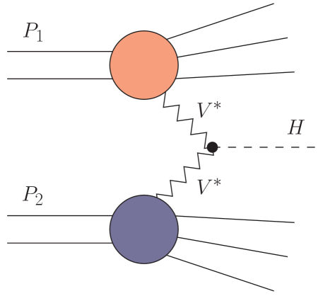
Figure 1.1: Illustration of Higgs production through vector boson fusion in the structure function approach. A vector boson is emitted from each of the two protons and fused into a Higgs boson. Each of the two protons are affected by separate but identical copies of QCD, here shown in orange and blue.

VBF is special for a number of reasons [13, 14, 4]:

• it has the largest cross section of the processes that involves tree-level production of the Higgs boson (and is second largest among all processes);

• it has a distinctive signature of two forward jets, which makes it possible to tag the events and so identify Higgs decays that normally have large backgrounds, e.g. $H\to\tau^{+}\tau^{-}$;

• the Higgs transverse momentum is non-zero even at lowest order, which facilitates searches for invisible decay modes [15, 16];

• and it also brings particular sensitivity to the charge-parity properties of the Higgs boson, and non-standard Higgs interactions, through the angular correlations of the forward jets [17].

The forward jets are due to the t-channel topology of the process. The overall energy of each jet is governed by the centre-of-mass energy of the collider whereas the transverse momentum of the jets are set by the mass of the weak vector bosons. For this reason VBF events also tend to have a large dijet invariant mass. These features make it possible to separate the VBF signal from the very large QCD background production through a set of cuts, which are usually referred to as VBF cuts. The VBF process therefore provides ideal access for the intricate measurements of the Higgs couplings [18].

Currently the VBF production signal strength has been measured with a precision of about 24% [19], though significant improvements can be expected during Run II and with the high luminosity LHC.

The unique topology of the VBF process makes it not just experimentally very accessible but also theoretically simple. One can view the VBF process as a double Deep Inelastic Scattering (DIS) process, where a vector boson is radiated independently from each proton after which the two vector bosons fuse into a Higgs boson. In this picture the matrix element factorises into the contraction of the two proton structure functions with the $HVV$ vertex, which is why it is known as the structure function approach [20]. The structure function approach is exact to NLO in the strong coupling constant and receives only tiny corrections from non-factorisable contributions beyond this order, which are both kinematically and colour suppressed. In fact, this approach is exact in the limit in which one considers that there are two identical copies of QCD associated with each of the two protons (shown orange and blue in Figure 1.1), whose interaction is mediated by the weak force.

Given the key role of VBF production at the LHC, it is of paramount importance to have a precise prediction for its production. The total VBF rate in the structure function approach was computed to NNLO some years ago  [21, 22, 23]. This calculation found NNLO corrections of about $1\%$ and renormalisation and factorisation scale uncertainties at the $5\permil$ level.

In this chapter we will first develop the structure function approach in some detail and then proceed to compute the N³LO QCD corrections to the total VBF cross section in this approximation. The calculation provides only the second N³LO calculation for processes of relevance to the LHC physics program, after a similar accuracy was recently achieved in the ggH channel [24]. However, unlike the ggH calculation, our calculation is fully differential in the Higgs kinematics. Since the NNLO corrections to VBF were already very small, the N³LO calculation is more of theoretical interest than of phenomenological. As we will see, the N³LO corrections are tiny and well within the scale uncertainty bands of the NNLO calculation. Hence our calculation shows very good convergence of perturbation theory for the VBF process.

Since our calculation gives access to the N³LO structure functions we also estimate missing higher order corrections to parton distribution functions, which are currently only know to NNLO. These corrections have not been studied in much detail yet, but are likely to become interesting as more processes become known at N³LO [25, 26].

1.1 The Structure Function Approach

In the structure function approach, as discussed above, the VBF Higgs production cross section is calculated as a double DIS process. Thus, it can be factorised as the product of the hadronic tensors $\mathcal{W}^{V}_{\mu\nu}$ and the matrix element for $V_{1}^{*}V_{2}^{*}\rightarrow H$, $\mathcal{M}^{\mu\nu}$. The cross section can be expressed by [20]

$$d\sigma= \frac{G_{F}^{2}}{s}M^{2}_{V_{1}}M^{2}_{V_{2}}\Delta_{V_{1}}^{2}(Q_{1}^{2})\Delta_{V_{2}}^{2}(Q_{2}^{2})\mathcal{W}^{V_{1}}_{\mu\nu}(x_{1},Q_{1}^{2})\mathcal{M}^{\mu\rho}\mathcal{M}^{*\nu\sigma}\mathcal{W}^{V_{2}}_{\rho\sigma}(x_{2},Q_{2}^{2})d\Omega_{\text{VBF}}.$$ (1.1)

Here $G_{F}$ is Fermi’s constant, $M_{V}$ is the mass of the vector boson, $\sqrt{s}$ is the collider centre-of-mass energy, $\Delta_{V}^{2}$ is the squared vector boson propagator, $Q_{i}^{2}=-q_{i}^{2}$ and $x_{i}=Q_{i}^{2}/(2P_{i}\cdot q_{i})$ are the usual DIS variables, and $d\Omega_{\text{VBF}}$ is the three-particle VBF phase space given by

$$d\Omega_{\text{VBF}}=\frac{d^{3}P_{4}}{(2\pi)^{3}2E_{4}}\frac{d^{3}P_{5}}{(2\pi)^{3}2E_{5}}ds_{4}ds_{5}\frac{d^{3}p_{3}}{(2\pi)^{3}2E_{3}}(2\pi^{4})\delta^{4}(P_{1}+P_{2}-p_{3}-P_{4}-P_{5}).$$ (1.2)

where $P_{1,2}$ are the incoming proton (not parton) momenta, $p_{3}$ is the momentum of the Higgs, $P_{4,5}$ are the outgoing proton remnant momenta, and $s_{i}=P_{i}^{2}=(P_{i-3}+q_{i-3})^{2}$ are the invariant masses of the proton remnants. From the knowledge of the vector boson momenta $q_{i}$, it is straightforward to reconstruct the Higgs momentum. As such, the cross section obtained using Equation 1.1 is differential in the Higgs kinematics. In the Standard Model, the $V_{1}^{*}V_{2}^{*}\rightarrow H$ matrix element is given by

$$\mathcal{M}^{\mu\nu}=2\sqrt{\sqrt{2}G_{F}}M_{V}^{2}g^{\mu\nu}.$$ (1.3)

The hadronic tensor $\mathcal{W}^{V}_{\mu\nu}$ can be expressed as

$$\mathcal{W}^{V}_{\mu\nu}(x_{i},Q_{i}^{2})=\Big{(}-g_{\mu\nu}+\frac{q_{i,\mu}q_{i,\nu}}{q_{i}^{2}}\Big{)}F_{1}^{V}(x_{i},Q_{i}^{2})\\ +\frac{\hat{P}_{i,\mu}\hat{P}_{i,\nu}}{P_{i}\cdot q_{i}}F_{2}^{V}(x_{i},Q_{i}^{2})+i\epsilon_{\mu\nu\rho\sigma}\frac{P_{i}^{\rho}q_{i}^{\sigma}}{2P_{i}\cdot q_{i}}F_{3}^{V}(x_{i},Q_{i}^{2})\,,$$ (1.4)

where we have defined $\hat{P}_{i,\mu}=P_{i,\mu}-\tfrac{P_{i}\cdot q_{i}}{q_{i}^{2}}q_{i,\mu}$, and the $F^{V}_{i}(x,Q^{2})$ functions are the standard DIS structure functions with $i=1,2,3$ and $V=Z,W^{-},W^{+}$ [27].

Since the matrix element in Equation 1.3 is proportional to the flat metric, it is obvious that the cross section must be proportional to the hadronic tensor contracted with itself. This contraction is given by

$$\mathcal{W}^{V_{1}}_{\mu\nu}(x_{1},Q_{1}^{2})\mathcal{W}^{V_{2},\mu\nu}(x_{2},Q_{2}^{2})=F_{1}^{V_{1}}F_{1}^{V_{2}}\left[2+\frac{(q_{1}\cdot q_{2})^{2}}{q_{1}^{2}q_{2}^{2}}\right]$$

$$+\frac{F_{1}^{V_{1}}F_{2}^{V_{2}}}{P_{2}\cdot q_{2}}\left[\frac{(P_{2}\cdot q_{2})^{2}}{q_{2}^{2}}+\frac{1}{q_{1}^{2}}\left(P_{2}\cdot q_{1}-\frac{(P_{2}\cdot q_{2})(q_{1}\cdot q_{2})}{q_{1}^{2}}\right)^{2}\right]$$

$$+\frac{F_{2}^{V_{1}}F_{1}^{V_{2}}}{P_{1}\cdot q_{1}}\left[\frac{(P_{1}\cdot q_{1})^{2}}{q_{1}^{2}}+\frac{1}{q_{2}^{2}}\left(P_{1}\cdot q_{2}-\frac{(P_{1}\cdot q_{1})(q_{1}\cdot q_{2})}{q_{2}^{2}}\right)^{2}\right]$$

$$+\frac{F_{2}^{V_{1}}F_{2}^{V_{2}}}{(P_{1}\cdot q_{1})(P_{2}\cdot q_{2})}\Bigg{[}P_{1}\cdot P_{2}-\frac{(P_{1}\cdot q_{1})(P_{2}\cdot q_{1})}{q_{1}^{2}}$$

$$\hskip 99.58464pt-\frac{(P_{1}\cdot q_{2})(P_{2}\cdot q_{2})}{q_{2}^{2}}+\frac{(P_{1}\cdot q_{1})(P_{2}\cdot q_{2})(q_{1}\cdot q_{2})}{q_{1}^{2}q_{2}^{2}}\Bigg{]}^{2}$$

$$+\frac{F_{3}^{V_{1}}F_{3}^{V_{2}}}{2(P_{1}\cdot q_{1})(P_{2}\cdot q_{2})}\left[(P_{1}\cdot P_{2})(q_{1}\cdot q_{2})-(P_{1}\cdot q_{2})(P_{2}\cdot q_{1})\right].$$ (1.5)

where we have dropped the argument $(x_{i},Q_{i}^{2})$ from the structure functions to ease notation.

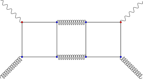
Figure 1.2: One of the new flavour structures appearing at N³LO for neutral current interactions but not charged current ones. Curly lines are gluons, wavy lines vector bosons and straight lines (anti)quarks.

In order to compute the NⁿLO cross section, we require the structure functions $F_{i}^{V}$ up to order $\mathcal{O}(\alpha_{s}^{n})$ in the strong coupling constant. Using the QCD factorisation theorem, we may express the structure functions as convolutions of the parton distribution functions (PDFs), $f_{a}$, with the short distance Wilson coefficient functions, $C_{i}$

$$F_{i}^{V}=\sum_{a=q,g}C_{i,a}^{V}\otimes f_{a}\,,\quad i=2,L,3\,,\quad V=Z,W^{+},W^{-}\,,$$ (1.6)

and

$$F_{L}^{V}=F_{2}^{V}-2xF_{1}^{V}.$$ (1.7)

All the necessary coefficient functions are known up to third order in the strong coupling constant . To compute the N³LO VBF Higgs production cross section, we therefore evaluate the convolution of the PDF with the appropriate coefficient functions in Equation 1.6. At N³LO, additional care is required due to the appearance of new flavour topologies [31], see Figure 1.2. Therefore, contributions corresponding to interference of diagrams where the vector boson attaches on different quark lines are to be set explicitly to zero for charged boson exchanges.

To that end, it is useful to decompose the quark and anti-quark distributions, $q_{i}(x,\mu)$ and $\bar{q}_{i}(x,\mu)$, into their pure-singlet contributions

$$q_{\text{PS}}=\sum_{i=1}^{n_{f}}(q_{i}+\bar{q}_{i})\,,$$ (1.8)

non-singlet valence contributions

$$q_{\text{NS}}^{v}=\sum_{i=1}^{n_{f}}(q_{i}-\bar{q}_{i})\,,$$ (1.9)

the flavour asymmetries

$$q_{\text{NS}}^{\pm}=(q_{i}\pm\bar{q}_{i})\,,$$ (1.10)

and the asymmetry $\delta q_{\text{NS}^{\pm}}$, which parametrises the isotriplet component of the proton

$$\delta q_{\text{NS}}^{\pm}=\sum_{i\in u\text{-type}}(q_{i}\pm\bar{q}_{i})-\sum_{i\in d-\text{type}}(q_{i}\pm\bar{q}_{i})\,.$$ (1.11)

We keep the gluon PDF, $g(x,Q^{2})$, as is.

This requires us to decompose the quark coefficient functions in a similar manner

$$C_{i,q}=C_{i,\text{NS}}^{+}+C_{i,\text{PS}},\quad i=2,L$$ (1.12)

and define the valence coefficient functions

$$C_{3,\text{NS}}^{v}=C_{3,\text{NS}}^{-}+C_{i,\text{NS}}^{s}.$$ (1.13)

Here the superscript $s$ denotes the “sea” contribution to the valence coefficient function. As it turns out, it is non-zero starting from third order, and the pure-singlet piece of Equation 1.12 is non-zero starting from second order [22].

With these definitions the neutral current structure functions take the form [22, 23]

$$F_{j}^{Z}(x,Q^{2}) =2x\int_{0}^{1}dz\int_{0}^{1}dy\delta(x-yz)\sum_{i=1}^{n_{f}}\left[v_{i}^{2}+a_{i}^{2}\right]$$

$$\quad\times\big{[}q_{\text{NS},i}^{+}(y,\mu_{F})C_{j,\text{NS}}^{+}(z,Q,\mu_{R},\mu_{F})$$

$$\quad\qquad+q_{\text{PS}}(y,\mu_{F})C_{j,\text{PS}}(z,Q,\mu_{R},\mu_{F})$$

$$\quad\qquad+g(y,\mu_{F})C_{j,g}(z,Q,\mu_{R},\mu_{F})\big{]},\quad j=2,L$$ (1.14)

$$F_{3}^{Z}(x,Q^{2}) =2\int_{0}^{1}dz\int_{0}^{1}dy\delta(x-yz)\sum_{i=1}^{n_{f}}2v_{i}a_{i}$$

$$\quad\times\big{[}q_{\text{NS},i}^{-}(y,\mu_{F})C_{3,\text{NS}}^{-}(z,Q,\mu_{R},\mu_{F})$$

$$\quad\qquad+q_{\text{NS}}^{v}(y,\mu_{F})C_{3,\text{NS}}^{s}(z,Q,\mu_{R},\mu_{F})\big{]}.$$ (1.15)

$v_{i}$ and $a_{i}$ are the vector and axial-vector couplings respectively. The needed combinations are given by

$$v_{i}^{2}+a_{i}^{2}=\begin{cases}\frac{1}{4}+\left(\frac{1}{2}-\frac{4}{3}\sin^{2}\theta_{W}\right)^{2},&\text{if }i\in u\text{-type quark}\\ \frac{1}{4}+\left(\frac{1}{2}-\frac{2}{3}\sin^{2}\theta_{W}\right)^{2},&\text{if }i\in d\text{-type quark}\end{cases}$$ (1.16)

and

$$2v_{i}a_{i}=\begin{cases}\frac{1}{2}-\frac{4}{3}\sin^{2}\theta_{W},&\text{if }i\in u\text{-type quark}\\ \frac{1}{2}-\frac{2}{3}\sin^{2}\theta_{W},&\text{if }i\in d\text{-type quark}\,.\end{cases}$$ (1.17)

For the charged current case the structure functions are given by

$$F_{j}^{W^{\pm}}(x,Q^{2}) =x\int_{0}^{1}dz\int_{0}^{1}dy\delta(x-yz)\frac{1}{n_{f}}\sum_{i=1}^{n_{f}}\left[v_{i}^{2}+a_{i}^{2}\right]$$

$$\quad\times\big{[}\mp\delta q_{\text{NS}}^{-}(y,\mu_{F})C_{j,\text{NS}}^{-}(z,Q,\mu_{R},\mu_{F})$$

$$\quad\qquad+q_{\text{PS}}(y,\mu_{F})C_{j,\text{q}}(z,Q,\mu_{R},\mu_{F})$$

$$\quad\qquad+g(y,\mu_{F})C_{j,g}(z,Q,\mu_{R},\mu_{F})\big{]},\quad j=2,L$$ (1.18)

$$F_{3}^{W^{\pm}}(x,Q^{2}) =\int_{0}^{1}dz\int_{0}^{1}dy\delta(x-yz)\sum_{i=1}^{n_{f}}2v_{i}a_{i}$$

$$\quad\times\big{[}\mp\delta q_{\text{NS},i}^{+}(y,\mu_{F})C_{3,\text{NS}}^{+}(z,Q,\mu_{R},\mu_{F})$$

$$\quad\qquad+q_{\text{NS}}^{v}(y,\mu_{F})C_{3,\text{NS}}^{v}(z,Q,\mu_{R},\mu_{F})\big{]}.$$ (1.19)

In this case the vector and axial-vector couplings are simply given by

$$v_{j}=a_{j}=\frac{1}{\sqrt{2}}.$$ (1.20)

These equations complete all the ingredients needed to evaluate the cross section in Equation 1.1. As previously noted, all coefficient functions are know to the precision of N³LO, whereas the PDFs themselves have only been determined to NNLO.

1.1.1 Scale Variation

The coefficient functions appearing above are in the literature expressed in terms of the vector boson momentum, $Q$. In general we are interested in computing the cross section for a range of different factorisation and renormalisation scales to asses the convergence of the perturbative series. In order to compute the dependence of the cross section on the values of the factorisation and renormalisation scales, we use renormalisation group methods [32, 33, 34] on the structure functions

$$F_{i}^{V}=\sum_{a}C_{i}^{V,a}\otimes f_{a}\,,\quad i=2,L,3\,.$$ (1.21)

This requires us to compute the scale dependence to third order in the coefficient functions as well as in the PDFs.

We start by evaluating the running coupling for $\alpha_{s}$ as an expansion in $\alpha_{s}$. This is done by iteratively solving the renormalisation group equation

$$\frac{d}{d\ln\mu^{2}}\alpha_{s}(\mu)=-\beta_{0}\alpha_{s}^{2}(\mu)-\beta_{1}\alpha_{s}^{3}(\mu)-\beta_{2}\alpha_{s}^{4}(\mu)-\beta_{3}\alpha_{s}^{5}(\mu)+\mathcal{O}(\alpha_{s}^{6})\,.$$ (1.22)

using

$$\alpha_{s}(Q)=\alpha_{s}({\mu_{\mathrm{R}}})-\int_{0}^{L_{RQ}}dL\frac{d}{dL}\alpha_{s}(\mu).$$ (1.23)

Integrating yields

$$\alpha_{s}(Q) =\alpha_{s}({\mu_{\mathrm{R}}})+\alpha_{s}^{2}({\mu_{\mathrm{R}}})\beta_{0}L_{RQ}+\alpha_{s}^{3}({\mu_{\mathrm{R}}})(\beta_{0}^{2}L_{RQ}^{2}+\beta_{1}L_{RQ})$$

$$+\alpha_{s}^{4}({\mu_{\mathrm{R}}})\left(\beta_{0}^{3}L_{RQ}^{3}+\frac{5}{2}\beta_{0}\beta_{1}L_{RQ}^{2}+\beta_{2}L_{RQ}\right)+\mathcal{O}(\alpha_{s}^{5}({\mu_{\mathrm{R}}}))\,,$$ (1.24)

where we introduced the shorthand notation

$$L_{RQ}=\ln\left(\frac{{\mu_{\mathrm{R}}}^{2}}{Q^{2}}\right)\,,\quad L_{FQ}=\ln\left(\frac{{\mu_{\mathrm{F}}}^{2}}{Q^{2}}\right)\,,\quad L=\ln\mu^{2}\,,$$ (1.25)

as well as [35, 36, 37, 38, 39]

$$4\pi\beta_{0} =11-\frac{2}{3}n_{f}$$

$$16\pi^{2}\beta_{1} =102-\frac{38}{3}n_{f}$$

$$64\pi^{3}\beta_{2} =\frac{2857}{2}-\frac{5033}{18}n_{f}+\frac{325}{54}n_{f}^{2}$$ (1.26)

where $n_{f}$ is the number of active flavours. We use the above to express the coefficient functions as an expansion in $\alpha_{s}(\mu_{R})$

$$C_{i}=\sum_{k=0}\left(\frac{\alpha_{s}(Q)}{2\pi}\right)^{k}C_{i}^{(k)}=C_{i}^{(0)}+\frac{\alpha_{s}({\mu_{\mathrm{R}}})}{2\pi}C_{i}^{(1)}+$$

$$\left(\frac{\alpha_{s}({\mu_{\mathrm{R}}})}{2\pi}\right)^{2}\left(C_{i}^{(2)}+2\pi\beta_{0}C_{i}^{(1)}L_{RQ}\right)+$$

$$\left(\frac{\alpha_{s}({\mu_{\mathrm{R}}})}{2\pi}\right)^{3}\bigg{[}C_{i}^{(3)}+4\pi\beta_{0}C_{i}^{(2)}L_{RQ}+4\pi^{2}C_{i}^{(1)}L_{RQ}(\beta_{1}+\beta_{0}^{2}L_{RQ})\bigg{]}+\mathcal{O}(\alpha_{s}^{4})\,.$$ (1.27)

To evaluate the dependence of the PDFs on the factorisation scale, ${\mu_{\mathrm{F}}}$, we integrate the DGLAP [40, 41, 42, 43] equation

$$\frac{d}{d\ln\mu^{2}}f(x,\mu)=\frac{\alpha_{s}(\mu)}{2\pi}(P\otimes f)(x,\mu)\,.$$ (1.28)

using

$$f(x,Q)=f(x,{\mu_{\mathrm{F}}})-\int_{0}^{L_{FQ}}dL\frac{d}{dL}f(x,\mu)\,.$$ (1.29)

Here both $P$ and $f$ are understood to be matrices expressed in terms of the singlet and non-singlet parts as above. The splitting kernels, $P$, can be expressed in terms of an expansion in $\alpha_{s}$

$$P(z,\alpha_{s})=\sum_{i=0}{\left(\frac{\alpha_{s}}{2\pi}\right)^{i}P^{(i)}(z)}\,,$$ (1.30)

where terms up to $P^{(2)}(z)$ are known [44, 45].

It is then straightforward to express the PDF evaluated at ${\mu_{\mathrm{F}}}$ in terms of an expansion in $\alpha_{s}({\mu_{\mathrm{R}}})$. Evaluating, we obtain

$$f(x,Q) =f(x,{\mu_{\mathrm{F}}})\Bigg{(}1-\frac{\alpha_{s}({\mu_{\mathrm{R}}})}{2\pi}L_{FQ}P^{(0)}$$

$$-\left(\frac{\alpha_{s}({\mu_{\mathrm{R}}})}{2\pi}\right)^{2}L_{FQ}\Big{[}P^{(1)}-\frac{1}{2}L_{FQ}(P^{(0)})^{2}-\pi\beta_{0}P^{(0)}(L_{FQ}-2L_{RQ})\Big{]}$$

$$-\left(\frac{\alpha_{s}({\mu_{\mathrm{R}}})}{2\pi}\right)^{3}L_{FQ}\Big{[}P^{(2)}-\frac{1}{2}L_{FQ}(P^{(0)}P^{(1)}+P^{(1)}P^{(0)})$$

$$\hskip 142.26378pt+\pi\beta_{0}(L_{FQ}-2L_{RQ})(L_{FQ}(P^{(0)})^{2}-2P^{(1)})$$

$$\hskip 142.26378pt+\frac{1}{6}L_{FQ}^{2}(P^{(0)})^{3}$$

$$\hskip 142.26378pt+4\pi^{2}\beta_{0}^{2}P^{(0)}(L_{RQ}^{2}-L_{FQ}L_{RQ}+\frac{1}{3}L_{FQ}^{2})$$

$$\hskip 142.26378pt-2\pi^{2}\beta_{1}P^{(0)}(L_{FQ}-2L_{RQ})\Big{]}+\mathcal{O}(\alpha_{s}^{4})\Bigg{)}\,.$$ (1.31)

where all the products are understood to be Mellin transforms

$$(f\otimes g)(x)=\int_{x}^{1}\frac{dy}{y}f(y)g(\frac{x}{y})\,.$$ (1.32)

Sections 1.1.1 and 1.1.1 allow us to evaluate the convolution in Equation 1.21 up to N³LO in perturbative QCD for any choice of the renormalisation and factorisation scales.

1.2 Impact of Higher Order PDFs

There is one source of formally N³LO QCD corrections appearing in Equation 1.6 which is currently unknown, namely missing higher order terms in the determination of the PDF. Indeed, in order to truly claim N³LO accuracy of the cross section we must use N³LO parton densities. However, only NNLO PDF sets are available at this time. These will be missing contributions from two main sources: from the higher order corrections to the coefficient functions that relate physical observables to PDFs; and from the higher order splitting functions in the evolution of the PDFs.

To evaluate the impact of future N³LO PDF sets on the total cross section, we consider two different approaches. A first, more conservative estimate, is to derive the uncertainty related to higher order PDF sets from the difference at lower orders, as described in [25] (see also [26]). We compute the NNLO cross section using both the NLO and the NNLO PDF set, and use their difference to extract the N³LO PDF uncertainty. We find in this way that at $13\;\mathrm{TeV}$ the uncertainty from missing higher orders in the extractions of PDFs is

$$\delta_{A}^{\text{PDF}}=\frac{1}{2}\left|\frac{\sigma^{\text{NNLO}}_{\text{NNLO-PDF}}-\sigma^{\text{NNLO}}_{\text{NLO-PDF}}}{\sigma^{\text{NNLO}}_{\text{NNLO-PDF}}}\right|=1.1\%\,.$$ (1.33)

Because the convergence is greatly improved going from NNLO to N³LO compared to one order lower, one might expect this to be rather conservative even with the factor half in Equation 1.33. Therefore, we also provide an alternative estimate of the impact of higher orders PDFs, using the known N³LO $F_{2}$ structure function.

We start by rescaling all the parton distributions using the $F_{2}$ structure function evaluated at a low scale $Q_{0}$

$$f^{\text{N${}^{3}$LO},\text{approx.}}(x,Q)=f^{\text{NNLO}}(x,Q)\frac{F_{2}^{\text{NNLO}}(x,Q_{0})}{F_{2}^{\text{N${}^{3}$LO}}(x,Q_{0})}\,.$$ (1.34)

In practice, we will use the $Z$ structure function. We then re-evaluate the structure functions in Equation 1.6 using the approximate higher order PDF given by Equation 1.34. This yields

$$\delta_{B}^{\text{PDF}}(Q_{0})=\left|\frac{\sigma^{\text{N${}^{3}$LO}}-\sigma^{\text{N${}^{3}$LO}}_{\text{rescaled}}(Q_{0})}{\sigma^{\text{N${}^{3}$LO}}}\right|=7.9\text{\permil}\,,$$ (1.35)

where in the last step, we used $Q_{0}=8\;\mathrm{GeV}$ and considered $13\;\mathrm{TeV}$ proton collisions.

By calculating a rescaled NLO PDF and evaluating the NNLO cross section in this way, we can evaluate the ability of this method to predict the corrections from NNLO PDFs. We find that with $Q_{0}=8\;\mathrm{GeV}$, the uncertainty estimate obtained in this way captures relatively well the impact of NNLO PDF sets.

The rescaled PDF sets obtained using Equation 1.34 will be missing N³LO corrections from the evolution of the PDFs in energy. We have checked the impact of these terms by varying the renormalisation scale up and down by a factor two around the factorisation scale in the splitting functions used for the PDF evolution. We find that the theoretical uncertainty associated with missing higher order splitting functions is less than one permille of the total cross section. Comparing this with Equation 1.35, it is clear that these effects are numerically subleading, suggesting that a practical alternative to full N³LO PDF sets could be obtained by carrying out a fit of DIS data using the hard N³LO matrix element.

The uncertainty estimates obtained with the two different methods described by Equations 1.33 and 1.35 are shown in Figure 1.3 as a function of centre-of-mass energy, and for a range of $Q_{0}$ values.

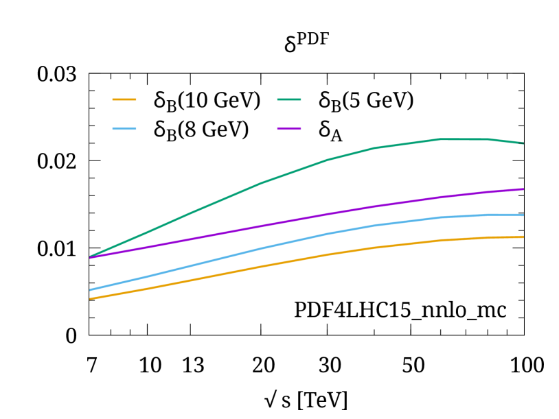
Figure 1.3: Estimate of the impact of missing higher orders corrections in PDFs, using Equations 1.33 and 1.35 with $Q_{0}=5$, $8$ and $10\;\mathrm{GeV}$.

One should note that the uncertainty estimates given in Equations 1.33 and 1.35 do not include what is usually referred to as PDF uncertainties. While we are here calculating missing higher order uncertainties to NNLO PDF sets, typical PDF uncertainties correspond to uncertainties due to errors on the experimental data and limitations of the fitting procedure. These can be evaluated for example with the PDF4LHC15 prescription [46], and are of about $2\%$ at $13\;\mathrm{TeV}$, which is larger than the corrections discussed above. One can also combine them with $\alpha_{s}$ uncertainties, which for VBF are at the $5\permil$ level. More detailed results on PDF and $\alpha_{s}$ uncertainties are given in Chapter 2.

1.3 Phenomenological Results

Let us now discuss in detail the phenomenological consequences of the N³LO corrections to VBF Higgs production. We present results for a wide range of energies in proton-proton collisions. The central factorisation and renormalisation scales appearing in the structure functions are set to the squared momentum of the corresponding vector boson. To estimate missing higher-order uncertainties, we use a seven-point scale variation, varying the scales by a factor two up and down while keeping $0.5<\mu_{R}/\mu_{F}<2$

$$\mu_{R,i}=\xi_{\mu_{R}}Q_{i}\,,\quad\mu_{F,i}=\xi_{\mu_{F}}Q_{i}\,,$$ (1.36)

where $\xi_{\mu_{R}},\xi_{\mu_{F}}\in\big{\{}\tfrac{1}{2},1,2\big{\}}$ and $i=1$, $2$ corresponds to the upper and lower hadronic sectors.

Our implementation uses the phase space from POWHEG’s two-jet VBF Higgs calculation [47]. The matrix element is derived from structure functions obtained with the parametrised DIS coefficient functions [48, 49, 50, 51, 52, 33, 53, 31, 54, 28], evaluated using HOPPET v1.2.0-devel [55]. We have tested our NNLO implementation against the results of one of the codes used in References [21, 22] and found agreement, both for the structure functions and the final cross sections. We have also checked that switching to the exact DIS coefficient functions has a negligible impact on both structure functions and total cross sections. A further successful comparison of the evaluation of NNLO structure functions was made against APFEL v.2.4.1[56].

For our computational setup, we use a diagonal CKM matrix with five light flavours ignoring top-quarks in the internal lines and final states. Full Breit-Wigner propagators for the $W$, $Z$ and the narrow-width approximation for the Higgs boson are applied. We use the PDF4LHC15_nnlo_mc PDF [46, 57, 58, 59] and four-loop evolution of the strong coupling [60], taking as our initial condition $\alpha_{s}(M_{Z})=0.118$. We set the Higgs mass to $M_{H}=125.09\;\mathrm{GeV}$, in accordance with the experimentally measured value [61]. Electroweak parameters are obtained from their PDG [62] values and tree-level electroweak relations. As inputs we use $M_{W}=80.385\;\mathrm{GeV}$, $M_{Z}=91.1876\;\mathrm{GeV}$ and $G_{F}=1.16637\times 10^{-5}\;\mathrm{GeV}^{-2}$. For the widths of the vector bosons we use $\Gamma_{W}=2.085\;\mathrm{GeV}$ and $\Gamma_{Z}=2.4952\;\mathrm{GeV}$.

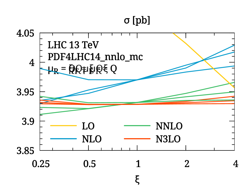
Figure 1.4: Dependence of the cross section on the renormalisation and factorisation scales for each order in perturbation theory.

To study the convergence of the perturbative series, we show in Figure 1.4 the inclusive cross section obtained at $13\;\mathrm{TeV}$ with $\mu_{R}=\mu_{F}=\xi Q$ for $\xi\in[1/4,4]$. Here we observe that at N³LO the scale dependence becomes extremely flat over the full range of renormalisation and factorisation scales. We note that similarly to the results obtained in the ggH channel [24], the convergence improves significantly at N³LO, with the N³LO prediction being well inside of the NNLO uncertainty band, while at lower orders there is a pattern of limited overlap of theoretical uncertainties.

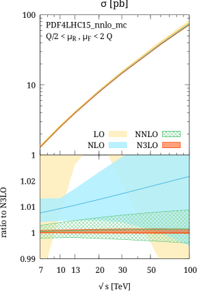
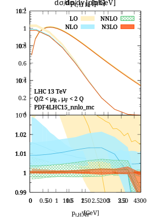
Figure 1.5: Cross section as a function of centre-of-mass energy (left), Higgs transverse momentum (centre) and Higgs rapidity (right).

In Figure 1.5 (left), we give the cross section as a function of centre-of-mass energy. We see that at N³LO the convergence of the perturbative series is very stable, with corrections of about $1\permil$ on the NNLO result. The scale uncertainty is dramatically reduced, going from $7\permil$ at NNLO to $1.4\permil$ at N³LO at $13\;\mathrm{TeV}$. A detailed breakdown of the cross section and scale uncertainty obtained at each order in QCD is given in Table 1.1 for $\sqrt{s}=13$, $14$ and $100\;\mathrm{TeV}$.

The centre and right plots of Figure 1.5 show the Higgs transverse momentum and rapidity distributions at each order in QCD, where we observe again a large reduction of the theoretical uncertainty at N³LO. The N³LO corrections are flat everywhere in phase space, except for at very high values of the Higgs rapidity.

x $\sigma^{(13\;\mathrm{TeV})}$ [pb] $\sigma^{(14\;\mathrm{TeV})}$ [pb] $\sigma^{(100\;\mathrm{TeV})}$ [pb] LO $4.099\,^{+0.051}_{-0.067}$ $4.647\,^{+0.037}_{-0.058}$ $77.17\,^{+6.45}_{-7.29}$ NLO $3.970\,^{+0.025}_{-0.023}$ $4.497\,^{+0.032}_{-0.027}$ $73.90\,^{+1.73}_{-1.94}$ NNLO $3.932\,^{+0.015}_{-0.010}$ $4.452\,^{+0.018}_{-0.012}$ $72.44\,^{+0.53}_{-0.40}$ N³LO $3.928\,^{+0.005}_{-0.001}$ $4.448\,^{+0.006}_{-0.001}$ $72.34\,^{+0.11}_{-0.02}$

Table 1.1: Inclusive cross sections at LO, NLO, NNLO and N³LO for VBF Higgs production. The quoted uncertainties correspond to scale variations $Q/2<{\mu_{\mathrm{R}}},{\mu_{\mathrm{F}}}<2Q$, while statistical uncertainties are at the level of $0.2\permil$.

A comment is due on non-factorisable QCD corrections. Indeed, for the results presented in this chapter, we have considered VBF in the usual DIS picture, ignoring diagrams that are not of the type shown in Figure 1.1. These effects neglected by the structure function approximation are known to contribute less than $1\%$ to the total cross section at NNLO [22]. The effects and their relative corrections are as follows:

• gluon exchanges between the upper and lower hadronic sectors, which appear at NNLO, but are kinematically and colour suppressed; These contributions along with the heavy-quark loop induced contributions have been estimated to contribute at the permille level [22];

• t-/u-channel interference which are known to contribute $\mathcal{O}(5\permil)$ at the fully inclusive level and $\mathcal{O}(0.5\permil)$ after VBF cuts have been applied [63];

• contributions from s-channel production, which have been calculated up to NLO [63]. At the inclusive level these contributions are sizeable but they are reduced to $\mathcal{O}(5\permil)$ after VBF cuts. The s-channel production is of course just associated Higgs production where the massive vector boson decays to a quark pair and hence it is usually considered a background process rather than an actual contribution to VBF;

• single-quark line contributions, which contribute to the VBF cross section at NNLO. At the fully inclusive level these amount to corrections of $\mathcal{O}(1\%)$ but are reduced to the permille level after VBF cuts have been applied [64];

• loop induced interference between VBF and ggH production. These contributions have been shown to be much below the permille level [65].

Furthermore, for phenomenological applications, one also needs to consider NLO electroweak effects [63], which amount to $\mathcal{O}(5\%)$ of the total cross section. In Chapter 2 we will study the impact of these electroweak corrections in some detail, and also investigate how big of an impact PDF uncertainties have on the total cross section.

1.4 Conclusions

In this chapter, we have presented the first N³LO calculation of a $2\to 3$ hadron-collider process, made possible by the DIS-like factorisation of the VBF process. This brings the precision of VBF Higgs production to the same formal accuracy as was recently achieved in the ggH channel in the heavy top mass approximation [24]. The N³LO corrections were found to be tiny, $1-2\permil$, and well within previous theoretical uncertainties, but they provide a large reduction of scale uncertainties, by a factor 5. Thus, although the corrections are sub-leading to many known effects omitted in the structure function approach, the calculation shows incredibly good convergence of perturbative QCD.

We also studied the impact of missing higher order corrections to the PDFs. We estimate that these corrections are at the $1\%$-level or below and that they are dominated by the hard process coefficient functions rather than unknown contributions to the splitting functions. Hence one could conceivably obtain approximate N³LO PDFs from DIS data and the known N³LO DIS coefficient functions. Our calculation also provides the first element towards a differential N³LO calculation for VBF Higgs production, which could be achieved through the projection-to-Born method (see Chapter 2) using an NNLO DIS 2+1 jet calculation [66, 67].

Chapter 2 Fully differential NNLO Vector Boson Fusion Higgs Production

In the previous chapter we saw how the total cross section for VBF Higgs production could be computed to N³LO using the structure function approach. The calculation has the obvious disadvantage of not being differential in the jet kinematics. The reason that the structure function approach does not provide a fully differential cross section, is related to the fact that the DIS coefficient functions used in the calculation implicitly integrate over hadronic final states. Whereas the Higgs boson momentum can be reconstructed from the knowledge of the momenta of the vector bosons emitted from the protons, only the momenta of the outgoing proton remnants are known and not those of the individual partons. In general it is therefore not possible to reconstruct the full final state momenta.

Given the smallness of the inclusive NNLO and N³LO corrections we may ask whether or not it is even relevant to study the differential corrections. In addition to that, the differential NLO corrections and their associated scale uncertainties have been known for a long time to be small [68]. However, because of the use of transverse-momentum cuts on the forward tagging jets, one might imagine that there are important NNLO corrections, associated with those jet cuts, that would not be seen in a fully inclusive calculation. As we shall see later, that is indeed the case.

In this chapter we eliminate the limitation of the structure function approach and present a fully differential NNLO calculation for VBF Higgs production. In order to do so, we will introduce the “projection-to-Born” method. An advantage of this approach is that it can be extended to any perturbative order and that it therefore opens up for a fully differential N³LO calculation as well. We proceed to present results relevant for the LHC and discuss the inclusion of electroweak corrections. At the end of the chapter, we discuss the prospects of studying VBF production at a $100\;\mathrm{TeV}$ proton-proton collider.

2.1 The “Projection-to-Born” Method

Let us start by recalling that the cross section in the structure function approach is expressed as a sum of terms involving products of structure functions, e.g. $F_{2}(x_{1},Q_{1}^{2})F_{2}(x_{2},Q_{2}^{2})$, where $Q_{i}^{2}=-q_{i}^{2}>0$ is given in terms of the 4-momentum $q_{i}$ of the (outgoing) exchanged vector boson $i$ (cf. Equations 1.1 and 1.5). The $x_{i}$ values are fixed by the relation

$$x_{i}=-\frac{Q_{i}^{2}}{(2P_{i}\cdot q_{i})}\,,$$ (2.1)

where $P_{i}$ is the momentum of proton $i$. To obtain the total cross section, one integrates over all $q_{1}$, $q_{2}$ that can lead to the production of a Higgs boson. If the underlying upper (lower) scattering is Born-like, $\mathrm{quark}\to\mathrm{quark}+V$, then it is straightforward to show that knowledge of the vector boson momentum $q_{1}$ ($q_{2}$) uniquely determines the momenta of both the incoming and outgoing (on-shell) quarks,

$$p_{\mathrm{in},i}=x_{i}P_{i},\qquad p_{\mathrm{out},i}=x_{i}P_{i}-q_{i}\,.$$ (2.2)

We exploit this feature in order to assemble a full calculation from two separate ingredients. For the first one, the “inclusive” ingredient, we remain within the structure function approach, and for each set of $q_{1}$ and $q_{2}$ use Equation 2.2 to assign VBF Born-like kinematics to the upper and lower sectors.

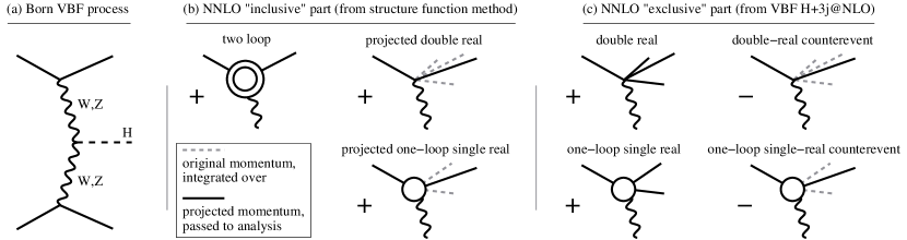
Figure 2.1: (a) Illustration of the Born VBF process. (b) NNLO corrections to the upper sector of the VBF process, from the “inclusive” part of our calculation. (c) Corresponding “exclusive” part. The double-real and one-loop single-real counterevents in the exclusive part cancel the projected double-real and one-loop single-real contributions in the inclusive part. In the “projected” and “counterevent” contributions, the dashed lines corresponds to the full set of parton momenta that are integrated over (for the structure functions, this integral is implicit in the derivation of the coefficient functions), while the solid lines correspond to the partons that are left over after projection to Born-like kinematics and then passed to the analysis. The projection does not change the direction of initial partons and so the corresponding incoming dashed lines are implicit.

This is represented in Figure 2.1b (showing just the upper sector): for the two-loop contribution, the Born kinematics that we assign corresponds to that of the actual diagrams; for the tree-level double-real and one-loop single-real diagrams, it corresponds to a projection from the true kinematics ($2\to H+n$ for $n=3,4$) down to the Born kinematics ($2\to H+2$). The projected momenta are used to obtain the “inclusive” contribution to differential cross sections. It is important to understand that in the structure function approach we are forced to construct the projected momenta rather than the full real and double-real momenta. As previously mentioned, this is due to the fact that the DIS coefficient functions are integrated over hadronic final state momenta.

Here we aim to replace the projected real and double-real contributions with their non-projected ones. We do so by adding a second, “exclusive”, ingredient to the “inclusive” one obtained from the structure function approach. This ingredient will contain the full real and double-real contributions plus a set of counterevents with projected kinematics. Let us first describe how to perform the projection starting from the full kinematics. For simplicity we will assume an event with only one real emission, see Figure 2.2. Such an event will have six external momenta, described by the vector

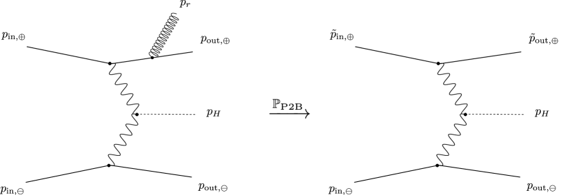
Figure 2.2: Illustration of the projection applied in the “projection-to-Born” method when there is only one radiated parton on the upper line. All the momenta before the projection are assumed known. The momenta of the Higgs, $p_{H}$ and the momenta on the lower line, $p_{\mathrm{in},\ominus}$ and $p_{\mathrm{out},\ominus}$, are all left invariant under the projection. The projected momenta, $\tilde{p}_{\mathrm{in},\oplus}$ and $\tilde{p}_{\mathrm{out},\oplus}$, are given in Equations 2.12 and 2.13.

$$\Omega_{R}=\left(p_{1},p_{2},p_{3},p_{4},p_{5},p_{6}\right)=\left(p_{\mathrm{in},\oplus},p_{\mathrm{in},\ominus},p_{H},p_{\mathrm{out},\oplus},p_{\mathrm{out},\ominus},p_{r}\right).$$ (2.3)

Here $\oplus$ ($\ominus$) refers to the upper (lower) VBF line and $p_{\mathrm{r}}$ is the radiated gluon. We define the projected momenta by

$$\mathbb{P}_{\mathrm{P2B}}\Omega_{R}=\Omega_{\mathrm{P2B}}=\left(\tilde{p}_{\mathrm{in},\oplus},\tilde{p}_{\mathrm{in},\ominus},p_{H},\tilde{p}_{\mathrm{out},\oplus},\tilde{p}_{\mathrm{out},\ominus}\right).$$ (2.4)

Let us now assume that the radiated particle is attached to the upper line of the VBF diagram. In order to ease notation we therefore drop the $\oplus$-subscript in the following. We then proceed to express the five momenta $p_{\mathrm{in}},p_{\mathrm{out}},p_{r},\tilde{p}_{\mathrm{in}},\tilde{p}_{\mathrm{out}}$ in lightcone coordinates

$$p=(p^{x},p^{y},p^{-},p^{+})\,,$$ (2.5)

where

$$p^{\pm}=\frac{1}{\sqrt{2}}(p^{E}\pm p^{z})\,,$$ (2.6)

and hence

$$p_{\mathrm{in}} =(0,0,0,p_{\mathrm{in}}^{+})$$ (2.7)

$$p_{\mathrm{out}} =(p_{\mathrm{out}}^{x},p_{\mathrm{out}}^{y},p_{\mathrm{out}}^{-},p_{\mathrm{out}}^{+})$$ (2.8)

$$p_{r} =(p_{r}^{x},p_{r}^{y},p_{r}^{-},p_{r}^{+})$$ (2.9)

$$\tilde{p}_{\mathrm{in}} =(0,0,0,\tilde{p}_{\mathrm{in}}^{+})$$ (2.10)

$$\tilde{p}_{\mathrm{out}} =(\tilde{p}_{\mathrm{out}}^{x},\tilde{p}_{\mathrm{out}}^{y},\tilde{p}_{\mathrm{out}}^{-},\tilde{p}_{\mathrm{out}}^{+})\,.$$ (2.11)

By momentum conservation we have

$$p_{\mathrm{in}}-p_{\mathrm{out}}-p_{r} =\tilde{p}_{\mathrm{in}}-\tilde{p}_{\mathrm{out}}\quad\Rightarrow\quad\begin{cases}\tilde{p}_{\mathrm{out}}^{x}=p_{\mathrm{out}}^{x}+p_{r}^{x}\\ \tilde{p}_{\mathrm{out}}^{y}=p_{\mathrm{out}}^{y}+p_{r}^{y}\\ \tilde{p}_{\mathrm{out}}^{-}=p_{\mathrm{out}}^{-}+p_{r}^{-}\\ \tilde{p}_{\mathrm{in}}^{+}=p_{\mathrm{in}}^{+}-p_{\mathrm{out}}^{+}-p_{r}^{+}+\tilde{p}_{\mathrm{out}}^{+}\,.\end{cases}$$ (2.12)

In order to find $\tilde{p}_{\mathrm{out}}^{+}$ we impose that the projected outgoing parton be massless

$$\left(\tilde{p}_{\mathrm{out}}\right)^{2} =0$$

$$\Rightarrow\quad\left(\tilde{p}_{\mathrm{out}}^{x}\right)^{2}+\left(\tilde{p}_{\mathrm{out}}^{y}\right)^{2}-2\tilde{p}_{\mathrm{out}}^{-}\tilde{p}_{\mathrm{out}}^{+}=0$$

$$\Rightarrow\quad\tilde{p}_{\mathrm{out}}^{+}=\frac{(p_{\mathrm{out}}^{x}+p_{r}^{x})^{2}+(p_{\mathrm{out}}^{y}+p_{r}^{y})^{2}}{2(p_{\mathrm{out}}^{-}+p_{r}^{-})}\,,$$ (2.13)

which fixes all the momenta. In order to find the projection when the radiated parton is on the lower line, we simply make the substitution $+\leftrightarrow-$ everywhere. At NNLO we will of course also have events with two radiated partons. In this case they can either both be attached to the same line or one on each line. In the former case we simply apply the projection above with $p_{r}$ as the sum of the the two radiated parton momenta. In the latter case we apply one projection to the upper line and one to the lower. Note that the Higgs momentum is unaffected by the projection under all circumstances.

The “exclusive” ingredient starts from the NLO fully differential calculation of vector boson fusion Higgs production with three jets [69, 70], as obtained in a factorised approximation, i.e. where there is no cross-talk between upper and lower sectors. Thus each parton can be uniquely assigned to one of the upper or lower sectors and the two vector boson momenta can be unambiguously determined. For each event in a Monte Carlo integration over phase space, with weight $w$, we add a counterevent, with weight $-w$, to which we assign projected Born VBF kinematics as given in Equations 2.12 and 2.13 and illustrated in Figures 2.1 and 2.2. From the original events, we thus obtain the full momentum structure for tree-level double-real and one-loop single-real contributions. Meanwhile, after integration over phase space, the counterevents exactly cancel the projected tree-level double-real and one-loop single-real contributions from the inclusive part of the calculation. Thus the sum of the “inclusive” and “exclusive” parts gives the complete differential NNLO VBF result.

2.2 Technical Implementation

For the implementation of the “inclusive” part of the calculation we use the implementation already described in Chapter 1. as a starting point for the “exclusive” part of the calculation, we took the NLO (i.e. fixed-order, but not parton-shower) part of the POWHEG $H$+3-jet VBF code [70], itself based on the calculation of Reference [69], with tree-level matrix elements from MadGraph 4 [72]. This code already uses a factorised approximation for the matrix element, however for a given phase-space point it sums over matrix-element weights for the assignments of partons to upper and lower sectors. We therefore re-engineered the code so that for each set of 4-momenta, weights are decomposed into the contributions for each of the four different possible sets of assignments of partons to the two sectors. For every element of this decomposition it is then possible to unambiguously obtain the vector boson momenta and so correctly generate a counterevent. The POWHEG-BOX’s [73, 74] “tagging” facility was particularly useful in this respect, notably for the NLO subtraction terms.

To check the correctness of the assignment to sectors, we verified that as the rapidity separation between the two leading jets increases, there was a decreasing relative fraction of the cross section for which partons assigned to the upper (lower) sector were found in the rapidity region associated with the lower (upper) leading jet, see Figure 2.3.

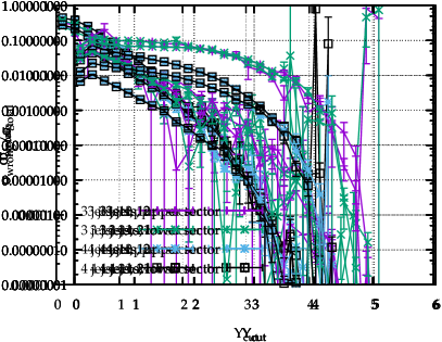
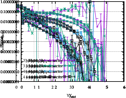
Figure 2.3: The relative fraction of the cross section for which partons assigned to the upper (lower) sector were found in the rapidity region associated with the lower (upper) leading jet as a function of the absolute rapidity separation of the two leading jets. We distinguish between events with 3 and 4 jets (anti-$k_{\scriptscriptstyle\mathrm{T}}$, $R=0.4$) and we separate between radiation on the upper and the lower line. Left: The distribution as found in our implementation. The relative fraction decreases exponentially with increasing rapidity separation. Right: Here we randomly re-assign the tags in the virtual correction, such that emissions sometimes end up in the wrong sector. The 3-jet distributions are clearly not decreasing anymore.

This figure also shows a similar plot, after a small bug was introduced in the program. The bug consisted of a random reassignment of tags, such that partons belonging to the upper (lower) sector was identified with the lower (upper) sector. We found that this bug gave visible results in the aforementioned distribution even when only a few percent of the partons were given the wrong tag. Furthermore, bugs of this type would ruin the internal POWHEG check of soft and collinear limits. We also tested that the sum of inclusive and exclusive contributions at NLO agrees with the POWHEG NLO implementation of the VBF $H$+2-jet process.

2.3 Phenomenological Results

To investigate the phenomenological consequences of the NNLO corrections, we study $13\;\mathrm{TeV}$ proton-proton collisions. We use a diagonal CKM matrix, full Breit-Wigners for the $W$, $Z$ and the narrow-width approximation for the Higgs boson. We take NNPDF 3.0 parton distribution functions at NNLO with $\alpha_{s}(M_{Z})=0.118$ (NNPDF30_nnlo_as_0118) [59], also for our LO and NLO results. We have five light flavours and ignore contributions with top-quarks in the final state or internal lines. We set the Higgs mass to $M_{H}=125\;\mathrm{GeV}$, compatible with the experimentally measured value [61]. Electroweak parameters are set according to known experimental values and tree-level electroweak relations. As inputs we use $M_{W}=80.398\;\mathrm{GeV}$, $M_{Z}=91.1876\;\mathrm{GeV}$ and $G_{F}=1.16637\times 10^{-5}\;\mathrm{GeV}^{-2}$. For the widths of the vector bosons we use $\Gamma_{W}=2.141\;\mathrm{GeV}$ and $\Gamma_{Z}=2.4952\;\mathrm{GeV}$.

Some care is needed with the renormalisation and factorisation scale choice. A natural option would be to use $Q_{1}$ and $Q_{2}$ as our central values for the upper and lower sectors, as in Chapter 1. While this is straightforward in the inclusive code, in the exclusive code we had the limitation that the underlying POWHEG-BOX code can presently only easily assign a single scale (or set of scales) to a given event. However, for each POWHEG phase-space point, we have multiple upper/lower classifications of the partons, leading to several $\{Q_{1},Q_{2}\}$ pairs for each event. Thus the use of $Q_{1}$ and $Q_{2}$ would require some further degree of modification of the POWHEG-BOX. We instead choose a central scale that depends on the Higgs transverse momentum $p_{\mathrm{T},H}$:

$$\mu_{0}^{2}(p_{\mathrm{T},H})=\frac{M_{H}}{2}\sqrt{\left(\frac{M_{H}}{2}\right)^{2}+p_{\mathrm{T},H}^{2}}\,.$$ (2.14)

This choice of $\mu_{0}$ is usually close to $\sqrt{Q_{1}Q_{2}}$ as is seen in Figure 2.4.

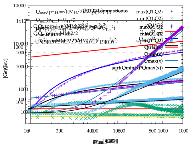
Figure 2.4: Our scale choice $\mu_{0}$ of Equation 2.14 (black) compared with $\sqrt{Q_{1}Q_{2}}$ (teal), $\mathrm{max}\{Q_{1},Q_{2}\}$ (purple), and $\mathrm{min}\{Q_{1},Q_{2}\}$ (green) as a function of the Higgs transverse momentum. Our scale choice is constructed as the product of two functions $Q_{\mathrm{max}}$ (blue) and $Q_{\mathrm{min}}$ (red) which approximate well the actual extrema.

It represents a good compromise between satisfying the requirement of a single scale for each event, while dynamically adapting to the structure of the event. In order to estimate missing higher-order uncertainties, we vary the renormalisation and factorisation scales symmetrically (i.e. keeping $\mu_{R}=\mu_{F}$) by a factor $2$ up and down around $\mu_{0}$. We verified that an expanded scale variation, allowing $\mu_{R}\neq\mu_{F}$ with $\frac{1}{2}<\mu_{R}/\mu_{F}<2$, led only to very small changes in the NNLO scale uncertainties for the VBF-cut cross section and the $p_{\mathrm{T},H}$ distribution, see Figure 2.5

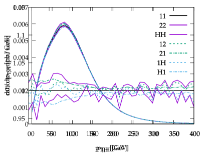
Figure 2.5: The transverse momentum of the Higgs boson evaluated at 7 different combinations of renormalisation, $\mu_{R}=K_{R}\mu_{0}$, and factorisation, $\mu_{F}=K_{F}\mu_{0}$, scales. The labels $XY$ refer to $K_{R}$ and $K_{F}$ in that order, where $H$ means half, i.e. $1/2$. Left: The differential cross section. Right: The ratio to the central scale, $11$. The 7-point scale variation is almost completely contained within the 3-point scale variation of $11,22$ and $HH$. If one takes the statistical fluctuations into account, the containment is perfect.

To pass our VBF selection cuts, events should have at least two jets with transverse momentum $p_{\scriptscriptstyle\mathrm{T}}>25\;\mathrm{GeV}$; the two hardest (i.e. highest $p_{\scriptscriptstyle\mathrm{T}}$) jets should have absolute rapidity $|y|<4.5$, be separated by a rapidity $\Delta y_{j_{1},j_{2}}>4.5$, have a dijet invariant mass $m_{j_{1},j_{2}}>600\;\mathrm{GeV}$ and be in opposite hemispheres ($y_{j_{1}}y_{j_{2}}<0$). Jets are defined using the anti-$k_{\scriptscriptstyle\mathrm{T}}$ algorithm [75], as implemented in FastJet v3.1.2 [76], with radius parameter $R=0.4$.

x $\sigma^{\mathrm{(nocuts)}}$ [pb] $\sigma^{\mathrm{(VBFcuts)}}$ [pb] LO $4.032\,^{+0.057}_{-0.069}$ $0.957\,^{+0.066}_{-0.059}$ NLO $3.929\,^{+0.024}_{-0.023}$ $0.876\,^{+0.008}_{-0.018}$ NNLO $3.888\,^{+0.016}_{-0.012}$ $0.826\,^{+0.013}_{-0.014}$

Table 2.1: Cross sections at LO, NLO and NNLO for VBF Higgs production, fully inclusively and with VBF cuts. The quoted uncertainties correspond to scale dependence, while statistical errors at NNLO are about $0.1\%$ with VBF cuts and much smaller without.

Results are shown in Table 2.1 for the fully inclusive cross section and with our VBF cuts. One sees that the NNLO corrections modify the fully inclusive cross section only at the percent level, which is compatible with the findings of Reference [21]. However, after VBF cuts, the NNLO corrections are about 5 times larger, reducing the cross section by $5-6\%$ relative to NLO. The magnitude of the NNLO effects after cuts imply that it will be essential to take them into account for future precision studies. Note that in both the inclusive and VBF-cut cases, the NNLO contributions are larger than would be expected from NLO scale variation.

Differential cross sections are shown in Figures 2.6 and 2.7, for events that pass the VBF cuts. We show in Figure 2.6 distributions of the transverse momentum of the two leading jets, $p_{\mathrm{T},j_{1}}$ and $p_{\mathrm{T},j_{2}}$, and in Figure 2.7 distributions of the Higgs boson transverse momentum, $p_{\mathrm{T},H}$, and the rapidity separation between the two leading jets, $\Delta y_{j_{1},j_{2}}$. The bands and the patterned boxes denote the scale uncertainties, while the vertical error-bars denote the statistical uncertainty. The effect of the NNLO corrections on the jets appears to be to reduce their transverse momentum, leading to negative (positive) corrections in regions of falling (rising) jet spectra. One can see effects of up to $10-12\%$. Turning to $p_{\mathrm{T},H}$, one might initially be surprised that such an inclusive observable should also have substantial NNLO corrections, of about $8\%$ for low and moderate $p_{\mathrm{T},H}$. Our interpretation is that since NNLO effects redistribute jets from higher to lower $p_{\scriptscriptstyle\mathrm{T}}$’s (cf. the plots for $p_{\mathrm{T},j_{1}}$ and $p_{\mathrm{T},j_{2}}$), they reduce the cross section for any observable defined with VBF cuts. As $p_{\mathrm{T},H}$ grows larger, the forward jets tend naturally to get harder and so automatically pass the $p_{\scriptscriptstyle\mathrm{T}}$ thresholds, reducing the impact of NNLO terms.

As observed above for the total cross section with VBF cuts, the NNLO differential corrections are sizeable and often outside the uncertainty band suggested by NLO scale variation. One reason for this might be that NLO is the first order where the non-inclusiveness of the jet definition matters, e.g. radiation outside the cone modifies the cross section. Thus NLO is, in effect, a leading-order calculation for the exclusive corrections, with all associated limitations.

Figure 2.6: From left to right, differential cross sections for the transverse momentum distributions for the two leading jets, $p_{\mathrm{T},j_{1}}$ and $p_{\mathrm{T},j_{2}}$.

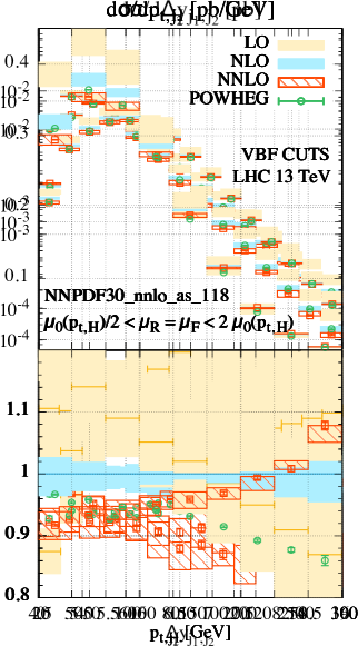
Figure 2.7: From left to right, differential cross sections for the transverse momentum distributions for the Higgs boson, $p_{\mathrm{T},H}$, and the distribution for the rapidity separation between the two leading jets, $\Delta y_{j_{1},j_{2}}$.

To further understand the size of the NNLO corrections, it is instructive to examine a NLO plus parton shower (NLOPS) calculation, since the parton shower will include some approximation of the NNLO corrections. For this purpose we have used the POWHEG VBF $H$+2-jet calculation [47], showered with PYTHIA version 6.428 with the Perugia 2012 tune [77]. The POWHEG part of this NLOPS calculation uses the same PDF, scale choices and electroweak parameters as our full NNLO calculation. The NLOPS results are included in Figures 2.6 and 2.7, at parton level, with multi-parton interactions (MPI) switched off. They differ from the NLO by an amount that is of a similar order of magnitude to the NNLO effects. This lends support to our interpretation that final (and initial)-state radiation from the hard partons is responsible for a substantial part of the NNLO corrections. However, while the NLOPS calculation reproduces the shape of the NNLO corrections for some observables (especially $p_{\mathrm{T},H}$), there are others for which this is not the case, the most striking being perhaps $\Delta y_{j_{1},j_{2}}$. Parton shower effects were also studied in Reference [78], using the MC@NLO approach [79]. Various parton showers differed there by up to about 10%. In addition to the NNLO contributions, precise phenomenological studies require the inclusion of electroweak (EW) contributions and non-perturbative hadronisation and MPI corrections. The former are of the same order of magnitude as our NNLO corrections [63]. Using Pythia 6.428 and Pythia 8.185 we find that hadronisation corrections are between $-2$ and $0\%$, while MPI brings up to $+5\%$ at low $p_{\scriptscriptstyle\mathrm{T}}$’s. The small hadronisation corrections appear to be due to a partial cancellation between shifts in $p_{\scriptscriptstyle\mathrm{T}}$ and rapidity.

2.3.1 Precision Studies for the LHC

Given that the effects mentioned above are of the same order as our NNLO corrections, it is useful to investigate their combined impact. In this section, we study in detail the combined effects of the NNLO QCD corrections presented here and EW contributions. In addition to that, we also study the effect of PDF and $\alpha_{s}$ uncertainties. The numerical results presented here have been computed using the values of the EW parameters given in Section 1.3. The electromagnetic coupling is fixed in the $G_{\scriptscriptstyle\mathrm{F}}$ scheme,

$$\alpha_{G_{\scriptscriptstyle\mathrm{F}}}=\sqrt{2}G_{\scriptscriptstyle\mathrm{F}}M_{\scriptscriptstyle\mathrm{W}}^{2}(1-M_{\scriptscriptstyle\mathrm{W}}^{2}/M_{\scriptscriptstyle\mathrm{Z}}^{2})/\pi,$$ (2.15)

and the weak mixing angle, $\theta_{\mathrm{w}}$, is defined in the on-shell scheme,

$$\sin^{2}\theta_{\mathrm{w}}=1-M_{\scriptscriptstyle\mathrm{W}}^{2}/M_{\scriptscriptstyle\mathrm{Z}}^{2}.$$ (2.16)

The renormalisation and factorisation scales are set equal to the $\mathup{{{W}}}$-boson mass,

$$\mu={\mu_{\mathrm{R}}}={\mu_{\mathrm{F}}}=M_{\scriptscriptstyle\mathrm{W}},$$ (2.17)

and both scales are varied in the range $M_{\scriptscriptstyle\mathrm{W}}/2<\mu<2M_{\scriptscriptstyle\mathrm{W}}$ keeping ${\mu_{\mathrm{F}}}={\mu_{\mathrm{R}}}$, which catches the full scale uncertainty of integrated cross sections (and of differential distributions in the essential regions). This fixed scale choice is a consequence of limitations in the implementation of the EW corrections.

The QCD corrections for inclusive cross sections and differential distributions have been obtained as described earlier in this chapter. EW corrections have been computed using HAWK [80, 81]. HAWK is a parton-level event generator for Higgs production in vector boson fusion [82, 63], $\mathup{{{p}}}\mathup{{{p}}}\to\mathup{{{H}}}+2\,\mathrm{jets}$, and Higgs-strahlung [83], $\mathup{{{p}}}\mathup{{{p}}}\to\mathup{{{H}}}\mathup{{{W}}}/\mathup{{{Z}}}\to\mathup{{{H}}}+2\,$leptons. It includes the complete NLO-QCD and EW corrections and all weak-boson fusion and quark–antiquark annihilation diagrams, i.e. $t$-channel and $u$-channel diagrams with VBF-like vector boson exchange and $s$-channel Higgs-strahlung diagrams with hadronic weak-boson decay, as well as all interferences. HAWK allows for an on-shell Higgs boson or for an off-shell Higgs boson (with optional decay into a pair of gauge singlets). The EW corrections include also the contributions from photon-induced channels, but contributions from effective Higgs–gluon couplings, which are part of the QCD corrections to Higgs production via gluon fusion, are not taken into account. External fermion masses are neglected and the renormalisation and factorisation scales are set to $M_{\scriptscriptstyle\mathrm{W}}$ by default. Since version 2.0, HAWK includes anomalous Higgs-boson–vector boson couplings. Further features of HAWK are described in [80] and on its web page [81].

In the calculation of the QCD-based cross sections, we have used the PDF4LHC15_nnlo_100 PDFs [46], for the calculation of the EW corrections we have employed the NNPDF2.3QED PDF set [84], which includes a photon PDF. Note, however, that the relative EW correction factor, which is used in the following, hardly depends on the PDF set, so that the uncertainty due to the mismatch in the PDF selection is easily covered by the other remaining theoretical uncertainties.

For the fiducial cross section and for differential distributions the following reconstruction scheme and cuts have been applied. Jets are constructed according to the anti-$k_{\scriptstyle\mathrm{T}}$ algorithm [75] with $R=0.4$. Jets are constructed from partons $j$ with

$$|\eta_{j}|<5\,,$$ (2.18)

where $\eta_{j}$ denotes the pseudo-rapidity. Real photons, which appear as part of the EW corrections, are an input to the jet clustering in the same way as partons. Thus, in real photon radiation events, final states may consist of jets only or jets plus a real identifiable photon, depending on whether the photon was merged into a jet or not, respectively. Both events with and without isolated photons are kept.

Jets are ordered according to their $p_{\scriptstyle\mathrm{T}}$ in decreasing progression. The jet with highest $p_{\scriptstyle\mathrm{T}}$ is called leading jet $(j_{1})$, the one with next highest $p_{\scriptstyle\mathrm{T}}$ subleading jet $(j_{2})$, and both are the tagging jets. Only events with at least two jets are kept. They must satisfy the additional constraints

$${p_{\scriptstyle\mathrm{T}}}_{j}>20\;\mathrm{GeV},\qquad|y_{j}|<5,\qquad|y_{j_{1}}-y_{j_{2}}|>3\,,\qquad M_{jj}>130\;\mathrm{GeV},$$ (2.19)

where $y_{j_{1,2}}$ are the rapidities of the two leading jets. The cut on the 2-jet invariant mass $M_{jj}$ is sufficient to suppress the contribution of $s$-channel diagrams to the VBF cross section to the level of $1{-}2\%$, so that the DIS approximation of taking into account only $t$- and $u$-channel contributions is justified. In the cross sections given below, the $s$-channel contributions will be given for reference, although they are not included in the final VBF cross sections by default.

While the VBF cross sections in the DIS approximation are independent of the CKM matrix, quark mixing has some effect on $s$-channel contributions. For the calculation of the latter we employed a Cabbibo-like CKM matrix (i.e. without mixing to the third quark generation) with Cabbibo angle, $\theta_{\mathrm{C}}$, fixed by $\sin\theta_{\mathrm{C}}=0.225$. Moreover, we note that we employ complex W- and Z-boson masses in the calculation of $s$-channel and EW corrections in the standard HAWK approach, as described in [82, 63].

The Higgs boson is treated as on-shell particle in the following consistently, since its finite-width and off-shell effects in the signal region are suppressed in the SM.

2.3.1.1 Integrated VBF Cross Sections

The final VBF cross section $\sigma^{\mathrm{VBF}}$ is calculated according to:

$$\sigma^{\mathrm{VBF}}=\sigma_{\text{NNLO}\mathrm{QCD}}^{\mathrm{DIS}}(1+\delta_{\mathrm{EW}})+\sigma_{\gamma},$$ (2.20)

where $\sigma_{\text{NNLO}\mathrm{QCD}}^{\mathrm{DIS}}$ is the NNLO-QCD prediction for the VBF cross section in DIS approximation with PDF4LHC15_nnlo_100 PDFs. The relative NLO EW correction $\delta_{\mathrm{EW}}$ is calculated with HAWK, but taking into account only $t$- and $u$-channel diagrams corresponding to the DIS approximation. The contributions from photon-induced channels, $\sigma_{\gamma}$, and from $s$-channel diagrams, $\sigma_{\mbox{\scriptsize$s$-channel}}$ are obtained from HAWK as well, where the latter includes NLO-QCD and EW corrections. To obtain $\sigma^{\mathrm{VBF}}$, the photon-induced contribution is added linearly, but $\sigma_{\mbox{\scriptsize$s$-channel}}$ is left out and only shown for reference, since it is not of true VBF origin (like other contributions such as H+2jet production via gluon fusion).

Tables 2.3 and 2.3 summarise the total and fiducial Standard Model VBF cross sections and the corresponding uncertainties for the different proton–proton collision energies for a Higgs-boson mass $M_{\scriptscriptstyle\mathrm{H}}=125\;\mathrm{GeV}$.

Table 2.2: Total VBF cross sections including QCD and EW corrections and their uncertainties for different proton–proton collision energies $\sqrt{s}$ for a Higgs-boson mass $M_{\scriptscriptstyle\mathrm{H}}=125\;\mathrm{GeV}$.

$\sqrt{s}$[GeV]	$\sigma^{\mathrm{VBF}}$[fb]	$\Delta_{\mathrm{scale}}$[%]	$\Delta_{\mathrm{PDF}/\alpha_{s}/\mathrm{PDF\oplus\alpha_{s}}}$[%]	$\sigma_{\text{NNLO}\mathrm{QCD}}^{\mathrm{DIS}}$[fb]	$\delta_{\mathrm{EW}}$[%]	$\sigma_{\gamma}$[fb]	$\sigma_{\mbox{\scriptsize$s$-channel}}$[fb]
$7$	$1241.4(1)$	${}^{+0.19}_{-0.21}$	$\pm 2.1/\pm 0.4/\pm 2.2$	$1281.1(1)$	$-4.4$	$17.1$	$584.5(3)$
$8$	$1601.2(1)$	${}^{+0.25}_{-0.24}$	$\pm 2.1/\pm 0.4/\pm 2.2$	$1655.8(1)$	$-4.6$	$22.1$	$710.4(3)$
$13$	$3781.7(1)$	${}^{+0.43}_{-0.33}$	$\pm 2.1/\pm 0.5/\pm 2.1$	$3939.2(1)$	$-5.3$	$51.9$	$1378.1(6)$
$14$	$4277.7(2)$	${}^{+0.45}_{-0.34}$	$\pm 2.1/\pm 0.5/\pm 2.1$	$4460.9(2)$	$-5.4$	$58.5$	$1515.9(6)$

Table 2.3: Fiducial VBF cross sections including QCD and EW corrections and their uncertainties for different proton–proton collision energies $\sqrt{s}$ for a Higgs-boson mass $M_{\scriptscriptstyle\mathrm{H}}=125\;\mathrm{GeV}$.

$\sqrt{s}$[GeV]	$\sigma^{\mathrm{VBF}}$[fb]	$\Delta_{\mathrm{scale}}$[%]	$\Delta_{\mathrm{PDF}/\alpha_{s}/\mathrm{PDF\oplus\alpha_{s}}}$[%]	$\sigma_{\text{NNLO}\mathrm{QCD}}^{\mathrm{DIS}}$[fb]	$\delta_{\mathrm{EW}}$[%]	$\sigma_{\gamma}$[fb]	$\sigma_{\mbox{\scriptsize$s$-channel}}$[fb]
$7$	$602.4(5)$	${}^{+1.3}_{-1.6}$	$\pm 2.3/\pm 0.3/\pm 2.3$	$630.8(5)$	$-6.1$	$9.9$	$8.2$
$8$	$795.9(6)$	${}^{+1.3}_{-1.5}$	$\pm 2.3/\pm 0.3/\pm 2.3$	$834.8(7)$	$-6.2$	$13.1$	$11.1$
$13$	$1975.4(9)$	${}^{+1.3}_{-1.2}$	$\pm 2.1/\pm 0.4/\pm 2.2$	$2084.2(10)$	$-6.8$	$32.3$	$29.0$
$14$	$2236.6(26)$	${}^{+1.5}_{-1.3}$	$\pm 2.1/\pm 0.4/\pm 2.1$	$2362.2(28)$	$-6.9$	$36.7$	$33.1$

The scale uncertainty, $\Delta_{\mathrm{scale}}$, results from a variation of the factorisation and renormalisation scales in Equation 2.17 by a factor of $2$ keeping ${\mu_{\mathrm{F}}}={\mu_{\mathrm{R}}}$, as indicated above, and the combined PDF${\oplus}\alpha_{s}$ uncertainty $\Delta_{\mathrm{PDF\oplus\alpha_{s}}}$ is obtained following the PDF4LHC recipe [46]. Both $\Delta_{\mathrm{scale}}$ and $\Delta_{\mathrm{PDF\oplus\alpha_{s}}}$ are actually obtained from $\sigma_{\text{NNLO}\mathrm{QCD}}^{\mathrm{DIS}}$, but these QCD-driven uncertainties can be taken over as uncertainty estimates for $\sigma^{\mathrm{VBF}}$ as well. The theoretical uncertainties of integrated cross sections originating from unknown higher-order EW effects can be estimated by

$$\Delta_{\mathrm{EW}}=\max\{0.5\%,\delta_{\mathrm{EW}}^{2},\sigma_{\gamma}/\sigma^{\mathrm{VBF}}\}.$$ (2.21)

The first entry represents the generic size of NNLO-EW corrections, while the second accounts for potential enhancement effects. Note that the whole photon-induced cross-section contribution $\sigma_{\gamma}$ is treated as uncertainty here, because the PDF uncertainty of $\sigma_{\gamma}$ is estimated to be $100\%$ with the NNPDF2.3QED PDF set. At present, this source, which is about $1.5\%$, dominates the EW uncertainty of the integrated VBF cross section.

2.3.1.2 Differential VBF Cross Sections

Figures 2.8, 2.9, 2.10, 2.11 and 2.12 show the most important differential cross sections for Higgs production via VBF in the SM.

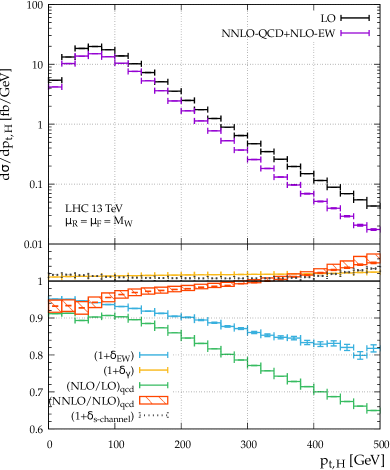
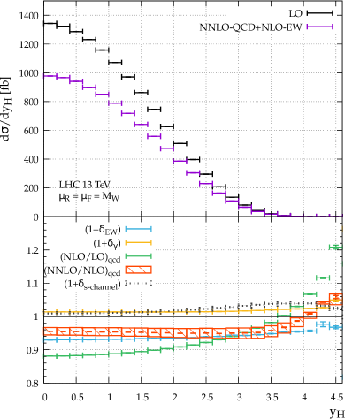
Figure 2.8: Transverse-momentum and rapidity distributions of the Higgs boson in VBF at LO and including NNLO-QCD and NLO-EW corrections (upper plots) and various relative contributions (lower plots) for $\sqrt{s}=13\;\mathrm{TeV}$ and $M_{\scriptscriptstyle\mathrm{H}}=125\;\mathrm{GeV}$.

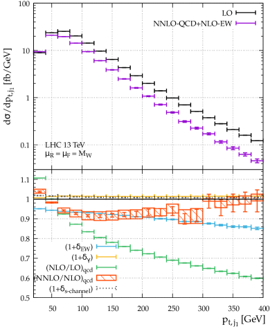
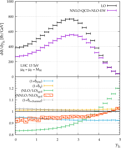
Figure 2.9: Transverse-momentum and rapidity distributions of the leading jet in VBF at LO and including NNLO-QCD and NLO-EW corrections (upper plots) and various relative contributions (lower plots) for $\sqrt{s}=13\;\mathrm{TeV}$ and $M_{\scriptscriptstyle\mathrm{H}}=125\;\mathrm{GeV}$.

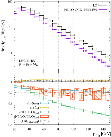
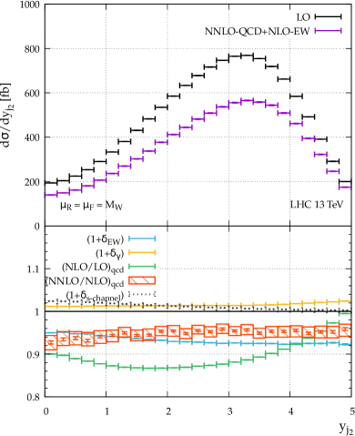
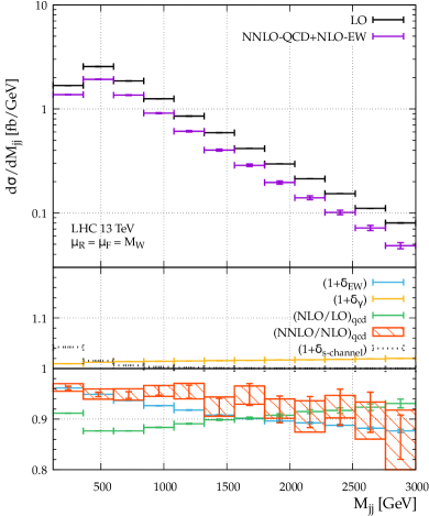
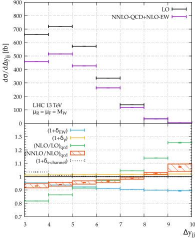
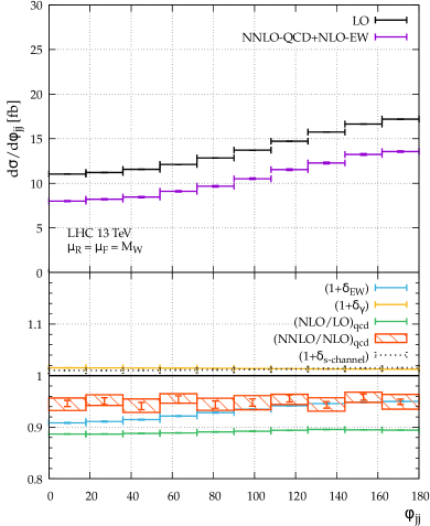
Figure 2.10: Transverse-momentum and rapidity distributions of the subleading jet in VBF at LO and including NNLO-QCD and NLO-EW corrections (upper plots) and various relative contributions (lower plots) for $\sqrt{s}=13\;\mathrm{TeV}$ and $M_{\scriptscriptstyle\mathrm{H}}=125\;\mathrm{GeV}$.

Figure 2.11: Distributions in the invariant mass and in the rapidity difference of the first two leading jets in VBF at LO and including NNLO-QCD and NLO-EW corrections (upper plots) and various relative contributions (lower plots) for $\sqrt{s}=13\;\mathrm{TeV}$ and $M_{\scriptscriptstyle\mathrm{H}}=125\;\mathrm{GeV}$.

Figure 2.12: Distribution in the azimuthal-angle difference of the first two leading jets in VBF at LO and including NNLO-QCD and NLO-EW corrections (upper plots) and various relative contributions (lower plots) for $\sqrt{s}=13\;\mathrm{TeV}$ and $M_{\scriptscriptstyle\mathrm{H}}=125\;\mathrm{GeV}$.

The upper panels show the LO cross section as well as the best fixed-order prediction, based on the analogue of Equation 2.20 for differential cross sections. The lower panels illustrate relative contributions and the ratios $(\text{NLO}/\text{LO})_{\mathrm{qcd}}$ and $(\text{NNLO}/\text{NLO})_{\mathrm{qcd}}$ of QCD predictions when going from LO to NLO-QCD to NNLO-QCD. Moreover, the relative EW correction to the (anti)quark–(anti)quark channels ($\delta_{\mathrm{EW}}=\sigma_{\mathrm{EW}}/\sigma_{\text{LO}}$) and the relative correction induced by initial-state photons ($\delta_{\gamma}=\sigma_{\gamma}/\sigma_{\text{LO}}$) are shown. Finally, the relative size of the $s$-channel contribution for Higgs+2jet production ($\delta_{\mbox{\scriptsize$s$-channel}}=\sigma_{\mbox{\scriptsize$s$-channel}}/\sigma_{\text{LO}}$) is depicted as well, although it is not included in the definition of the VBF cross section. Integrating the differential cross sections shown in the following, and all its individual contributions, results in the fiducial cross sections discussed in the previous section.

The ratio $(\text{NLO}/\text{LO})_{\mathrm{qcd}}$ shows a quite large impact of NLO-QCD corrections, an effect that can be traced back to the scale choice $\mu=M_{\scriptscriptstyle\mathrm{W}}$, which is on the low side if mass scales such as $p_{\mathrm{T}}$ and $M_{jj}$ get large in some distributions. The moderate ratio $(\text{NNLO}/\text{NLO})_{\mathrm{qcd}}$, however, indicates nice convergence of perturbation theory at NNLO-QCD. The band around the ratio $(\text{NNLO}/\text{NLO})_{\mathrm{qcd}}$ illustrates the scale uncertainty of the NNLO-QCD cross section, which also applies to $\sigma^{\mathrm{VBF}}$.

The EW corrections $\delta_{\mathrm{EW}}$ to (pseudo)rapidity and angular distributions are rather flat, resembling the correction to the integrated (fiducial) cross section. In the high-energy tails of the $p_{\mathrm{T}}$ and $M_{jj}$ distributions, $\delta_{\mathrm{EW}}$ increases in size to $10$–$20\%$, showing the onset of the well-known large negative EW corrections that are enhanced by logarithms of the form $(\alpha/\sin\theta_{\mathrm{W}}^{2})\ln^{2}(p_{\mathrm{T}}/M_{\scriptscriptstyle\mathrm{W}})$. The impact of the photon-induced channels uniformly stays at the generic level of $1$–$2\%$, i.e. they cannot be further suppressed by cuts acting on the variables shown in the distributions.

The contribution of $s$-channel (i.e. VH-like) production uniformly shows the relative size of about $1.5\%$ observed in the fiducial cross section, with the exception of the $M_{jj}$ and $\Delta y_{jj}$ distributions, where this contribution is enhanced at the lower ends of the spectra. Tightening the VBF cuts at these ends, would further suppress the impact of $\sigma_{s-\mathrm{channel}}$, but reduce the signal at the same time. As an alternative to decreasing $\sigma_{s-\mathrm{channel}}$, a veto on subleading jet pairs with invariant masses around $M_{\scriptscriptstyle\mathrm{W}}$ or $M_{\scriptscriptstyle\mathrm{Z}}$ may be promising. Such a veto, most likely, would reduce the photon-induced contribution $\delta_{\gamma}$, and thus the corresponding uncertainty, as well.

The theoretical uncertainties of differential cross sections originating from unknown higher-order EW effects can be estimated by

$$\Delta_{\mathrm{EW}}=\max\{1\%,\delta_{\mathrm{EW}}^{2},\sigma_{\gamma}/\sigma^{\mathrm{VBF}}\},$$ (2.22)

i.e. $\Delta_{\mathrm{EW}}$ is taken somewhat more conservative than for integrated cross sections, accounting for possible enhancements of higher-order effects due to a kinematical migration of events in distributions. Note that $\delta_{\mathrm{EW}}^{2}$, in particular, covers the known effect of enhanced EW corrections at high momentum transfer (EW Sudakov logarithms, etc.). As discussed for integrated cross sections in the previous section, the large uncertainty of the current photon PDF forces us to include the full contribution $\sigma_{\gamma}$ in the EW uncertainties.

2.3.2 Future Circular Collider Studies

In this section we study the production of a Standard Model Higgs boson through vector boson fusion at a $100\;\mathrm{TeV}$ proton-proton collider. As is the case at $13\;\mathrm{TeV}$, VBF has the second largest Higgs production cross section and is interesting on its own for a multitude of reasons: 1) it is induced already at tree-level; 2) the transverse momentum of the Higgs is non-zero at lowest order which makes it suitable for searches for invisible decays; 3) it can be distinguished from background processes due to a signature of two forward jets. This last property is very important, as the inclusive VBF signal is completely drowned in QCD background. One of the aims of this section is to study how well typical VBF cuts suppress this background at a $100\;\mathrm{TeV}$ proton-proton machine. In contrast to previous sections, we will here therefore also study Higgs plus 2 jets production in the gluon fusion channel (QCD $Hjj$).

2.3.2.1 Generators

Fixed order QCD and EW predictions have been obtained in the same way as in previous sections. NLO interfaced to a parton shower (NLOPS) results have been obtained using the POWHEG-BOX [47, 73, 86, 74] together with version 6.428 of PYTHIA [87] with the Perugia Tune P12 [77]. LO QCD $Hjj$ results are obtained from the POWHEG-BOX using the fixed-order part of [88]. The NLO QCD $Hjj$ predictions have been obtained by using the setup developed for an analogous analysis at $8$ and $13\;\mathrm{TeV}$ [89], and is based on the automated tools GoSam [90, 91] and Sherpa [92], linked via the interface defined in the Binoth Les Houches Accord [93, 94].

The one-loop amplitudes are generated with GoSam, and are based on an algebraic generation of $d$-dimensional integrands using a Feynman diagrammatic approach. The expressions for the amplitudes are generated employing QGraf [95], Form [96, 97] and Spinney [98]. For the reduction of the tensor integrals at running time, we used Ninja [99, 100], which is an automated package carrying out the integrand reduction via Laurent expansion [101], and OneLoop [102] for the evaluation of the scalar integrals. Unstable phase space points are detected automatically and reevaluated with the tensor integral library Golem95 [103, 104, 105]. The tree-level matrix elements for the Born and real-emission contribution, and the subtraction terms in the Catani-Seymour approach [106] have been evaluated within Sherpa using the matrix element generator Comix [107].

Using this framework we stored NLO events in the form of Root Ntuples. Details about the format of the Ntuples generated by Sherpa can be found in Reference [108]. The predictions presented in the following were computed using Ntuples at $14$ and $100\;\mathrm{TeV}$ with generation cuts specified by

$$p_{T,\,\mathrm{jet}}\;>\;25\>\mathrm{GeV}\qquad\mbox{and}\qquad|\eta_{\mathrm{jet}}|\;<\;10\,,$$

and for which the Higgs boson mass $M_{\scriptscriptstyle\mathrm{H}}$ and the Higgs vacuum expectation value $v$ are set to $M_{\scriptscriptstyle\mathrm{H}}=125\>\mathrm{GeV}$ and $v=246\>\mathrm{GeV}$, respectively. To improve the efficiency in performing the VBF analysis using the selection cuts described below, a separate set of Ntuples was generated. This set includes an additional generation cut on the invariant mass of the two leading transverse momentum jets. To generate large dijet masses from scratch, we require $M_{jj}>1600\>\mathrm{GeV}$.

2.3.2.2 Parameters

The setup for this study is identical to the one used in the previous section except that for VBF predictions we have used the MMHT2014nnlo68cl [58] PDF set and for QCD $Hjj$ predictions we have used the CT14nnlo [57] PDF set as implemented in LHAPDF [109].

In order to estimate scale uncertainties we vary $\mu$ up and down a factor $2$ while keeping $\mu_{R}=\mu_{F}$. For QCD VBF results we use the scale choice of Equation 2.14, for EW predictions we use $M_{\scriptscriptstyle\mathrm{W}}$ as central scale and for QCD $Hjj$ predictions we use $\hat{H}^{\prime}_{\mathrm{T}}/2$ as our central scale defined as

$$\frac{\hat{H}^{\prime}_{T}}{2}\;=\;\frac{1}{2}\left(\sqrt{M_{\scriptscriptstyle\mathrm{H}}^{2}+p_{T,H}^{2}}+\sum_{i}|p_{T,\,j_{i}}|\right)\,.$$ (2.23)

The sum runs over all partons accompanying the Higgs boson in the event.

2.3.2.3 Inclusive VBF Production

Due to the massive vector bosons exchanged in VBF production the cross section is finite even when both jets become fully unresolved in fixed-order calculations. In Table 2.4 we present the fully inclusive LO VBF cross section and both NNLO-QCD and NLO-EW corrections at a $100\;\mathrm{TeV}$ proton-proton collider.

Table 2.4: Total VBF cross section including QCD and EW corrections and their uncertainties for a $100\;\mathrm{TeV}$ proton-proton collider. $\sigma^{\mathrm{VBF}}$ is obtained using Equation 2.20 where $\sigma_{\mathrm{NNLO-QCD}}^{\mathrm{DIS}}$ is the total VBF cross section computed to NNLO accuracy in QCD, $\delta_{\mathrm{EW}}$ is the relative EW induced corrections and $\sigma_{\gamma}$ is the cross section induced by incoming photons. For comparison, the LO order cross section, $\sigma_{\mathrm{LO}}$, is also shown.

$\sigma^{\mathrm{VBF}}$[pb]	$\Delta_{\mathrm{scale}}$[%]	$\sigma_{\mathrm{LO}}$[pb]	$\sigma_{\mathrm{NNLO-QCD}}^{\mathrm{DIS}}$[pb]	$\delta_{\mathrm{EW}}$[%]	$\sigma_{\gamma}$[pb]
$69.0$	${}^{+0.85}_{-0.46}$	$80.6$	$73.5$	$-7.3$	$0.81$

In order to compute the VBF cross section we combine the NNLO-QCD and NLO-EW corrections according to Equation 2.20.

The combined corrections to the LO cross section is about $14\%$ with QCD and EW corrections contributing an almost equal amount. The scale uncertainty $\Delta_{\mathrm{scale}}$ is due to varying $\mu$ by a factor $2$ up and down in the QCD calculation alone keeping $\mu_{F}=\mu_{R}$. For comparison the total QCD and EW corrections at $14\;\mathrm{TeV}$ amount to about $7\%$ and the QCD induced scale variations to about $0.4\%$, cf. Table 2.3.

2.3.2.4 VBF Cuts

In order to separate the VBF signal from the main background of QCD $Hjj$ production we will extend typical VBF cuts used at the LHC to a $100\;\mathrm{TeV}$ proton-proton collider. These cuts take advantage of the fact that VBF Higgs production, and VBF production in general, has a very clear signature of two forward jets clearly separated in rapidity. Examining the topology of a typical VBF production diagram it becomes very clear that this is the case because the two leading jets are essential remnants of the two colliding protons. Since the $p_{\scriptscriptstyle\mathrm{T}}$ of the jets will be governed by the mass scale of the weak vector bosons and the energy by the PDFs the jets will typically be very energetic and in opposite rapidity hemispheres.

Figure 2.13: Left panel: The $p_{\scriptscriptstyle\mathrm{T}}$ of the hardest jet in VBF production at $100\;\mathrm{TeV}$. We require at least two jets in the event but apply no other cuts; right panel: The $p_{\scriptscriptstyle\mathrm{T}}$ of the second hardest jet in VBF and QCD $Hjj$ production at $100\;\mathrm{TeV}$.

As is clear from Figure 2.13 the hardest jet in VBF production peaks at around $60\;\mathrm{GeV}$. As discussed above, this value is set by the mass of the weak vector bosons and hence the $p_{\scriptscriptstyle\mathrm{T}}$ spectra of the two hardest jets are very similar to what one finds at the LHC. From this point of view, and in order to maximise the VBF cross section, one should keep jets with $p_{\mathrm{T},cut}>30\;\mathrm{GeV}$. Here we present results for $p_{\mathrm{T},cut}=\{30,50,100\}\;\mathrm{GeV}$ to study the impact of the jet cut on both the VBF signal and QCD $Hjj$ background. We only impose the cut on the two hardest jets in the event.

To establish VBF cuts at $100\;\mathrm{TeV}$ we first study the variables which are typically used at the LHC. These are the dijet invariant mass, $M_{jj}$, the rapidity separation between the two leading jets, $\Delta y_{jj}$, the separation between the two leading jets in the rapidity-azimuthal angle plane, $\Delta R_{jj}$ and the azimuthal angle between the two leading jets $\phi_{jj}$. In Figure 2.14 we show $M_{jj}$ and $\Delta y_{jj}$ after applying a cut on the two leading jets of $p_{\scriptscriptstyle\mathrm{T}}>30\;\mathrm{GeV}$ and requiring that the two leading jets are in opposite detector hemispheres. This last cut removes around $60\%$ of the background while retaining about $80\%$ of the signal.

Figure 2.14: Left: The invariant dijet mass $M_{jj}$ of the two hardest jets in VBF and QCD $Hjj$ production at $100\;\mathrm{TeV}$. Right: The rapidity separation of the two hardest jets $\Delta y_{jj}$ in VBF and QCD $Hjj$ production at $100\;\mathrm{TeV}$.

In order to suppress the QCD background a cut of $\Delta y_{jj}>6.5$ is imposed. This cut also significantly reduces the QCD $M_{jj}$ peak and shifts the VBF peak to about $2400\;\mathrm{GeV}$. In order to further suppress the QCD background we impose $M_{jj}>1600\;\mathrm{GeV}$. After these cuts have been applied, and requiring $p_{\mathrm{T},j}>30\;\mathrm{GeV}$, the VBF signal to QCD background ratio is roughly 3 with a total NNLO-QCD VBF cross section of about $12$ pb. From Figure 2.15 it is clear that one could also impose a cut on $\phi_{jj}$ to improve the suppression whereas a cut on $\Delta R_{jj}$ would not help to achieve that. We hence state the VBF cuts that we will be using throughout this section are

$$M_{j_{1}j_{2}}>1600\;\mathrm{GeV},\qquad\Delta y_{j_{1}j_{2}}>6.5,\qquad y_{j_{1}}y_{j_{2}}<0.$$ (2.24)

where $j_{1}$ is the hardest jet in the event and $j_{2}$ is the second hardest jet. At a $13\;\mathrm{TeV}$ machine the VBF cross section is $\mathcal{O}(1\;\mathrm{pb})$ under typical VBF cuts and the QCD $Hjj$ background roughly a factor six smaller.

Figure 2.15: Left: The azimuthal angle $\phi_{jj}$ between the two hardest jets in VBF and QCD $Hjj$ production at $100\;\mathrm{TeV}$. Right: The rapidity-azimuthal angle separation of the two hardest jets $\Delta R_{jj}$ in VBF and QCD $Hjj$ production at $100\;\mathrm{TeV}$.

In Table 2.5 we show the fiducial cross section obtained after applying the VBF cuts of Equation 2.24 to VBF and QCD $Hjj$ production. The cross sections are reported at the three different jet $p_{\scriptscriptstyle\mathrm{T}}$ cut values $\{30,50,100\}\;\mathrm{GeV}$. All numbers are computed at LO. It is clear from the table that requiring a somewhat higher jet $p_{\scriptscriptstyle\mathrm{T}}$ cut than $30\;\mathrm{GeV}$ leads to a lower $S/\sqrt{B}$ ratio. In going from $30\;\mathrm{GeV}$ to $50\;\mathrm{GeV}$ this reduction is however small.

Table 2.5: Fiducial VBF and QCD $Hjj$ cross sections for a $100\;\mathrm{TeV}$ proton-proton collider at LO under the VBF cuts of Equation 2.24. $S/\sqrt{B}$ is defined as the ratio between the VBF signal and the square root of the QCD background at an integrated luminosity of $20\mbox{ ab}^{-1}$.

	$\sigma(p_{\mathrm{T},j}>30\;\mathrm{GeV})$ [pb]	$\sigma(p_{\mathrm{T},j}>50\;\mathrm{GeV})$ [pb]	$\sigma(p_{\mathrm{T},j}>100\;\mathrm{GeV})$ [pb]
VBF	$14.1$	$7.51$	$1.08$
QCD $Hjj$	$5.04$	$1.97$	$0.331$
$S/\sqrt{B}@(20\mbox{ ab}^{-1})$	$28100$	$24200$	$8500$

In Table 2.6 we show for comparison the cross sections obtained after only applying the three jet $p_{\scriptscriptstyle\mathrm{T}}$ cuts. As expected the VBF signal is drowned in the QCD background. It is worth noticing that the $S/\sqrt{B}$ ratio is still very large when one assumes an integrated luminosity of $20\mbox{ ab}^{-1}$ and that it declines as the jet cut is increased.

Table 2.6: Total VBF and QCD $Hjj$ cross sections for a $100\;\mathrm{TeV}$ proton-proton collider at LO with a cut on the two hardest jets. The numbers are obtained using the CT14nnlo PDF. $S/\sqrt{B}$ is defined as the ratio between the VBF signal and the square root of the QCD background at an integrated luminosity of $20\mbox{ ab}^{-1}$.

	$\sigma(p_{\mathrm{T},j}>30\;\mathrm{GeV})$ [pb]	$\sigma(p_{\mathrm{T},j}>50\;\mathrm{GeV})$ [pb]	$\sigma(p_{\mathrm{T},j}>100\;\mathrm{GeV})$ [pb]
VBF	$51.3$	$28.5$	$5.25$
QCD $Hjj$	$166$	$78.6$	$23.9$
$S/\sqrt{B}@(20\mbox{ ab}^{-1})$	$17900$	$14300$	$4900$

2.3.2.5 Perturbative Corrections

The results shown in the previous section were all computed at LO. Here we briefly investigate the impact of NNLO-QCD, NLO-EW and parton shower corrections to the VBF cross section computed with $p_{\mathrm{T},j}>30\;\mathrm{GeV}$ and under the VBF cuts of Equation 2.24 at a $100\;\mathrm{TeV}$ collider. We also compare to the NLO-QCD predictions for QCD $Hjj$ production.

In Table 2.7 we show the best prediction for $\sigma^{\mathrm{VBF}}$ as obtained by Equation 2.20 and compare it to the same cross section obtained by showering POWHEG events with PYTHIA6 but including no effects beyond the parton shower itself. The NLO-EW and NNLO-QCD corrections are found to be of roughly the same order, and amount to a total negative correction of $\sim 23\%$. As was the case for the inclusive cross section, the corrections are a factor two larger than at $14\;\mathrm{TeV}$. Even though the perturbative corrections to QCD $Hjj$ production are negative, the effect of including higher order corrections to both VBF and QCD $Hjj$ production is that the $S/\sqrt{B}$ ratio at an integrated luminosity of $20\mbox{ ab}^{-1}$ is decreased from $28100$ to $24300$.

Table 2.7: Fiducial VBF cross section including QCD and EW corrections and their uncertainties for a $100\;\mathrm{TeV}$ proton-proton collider. For comparison the QCD induced Hjj cross section is also shown. At fixed-order QCD corrections are included at NNLO and EW corrections at NLO.

Process	$\sigma^{\mathrm{fid}}$[pb]	$\Delta_{\mathrm{scale}}$[%]	$\sigma_{\mathrm{QCD}}$[pb]	$\delta_{\mathrm{EW}}$[%]	$\sigma_{\gamma}$[pb]
VBF (NNLO-QCD/NLO-EW)	$10.8$	$\pm 1.0$	$12.1$	$-12.6$	$0.22$
VBF (NLOPS)	$11.9$	${}^{+0.56}_{-0.41}$	$11.9$	-	-
QCD $Hjj$ (NLO)	$4.79$	${}^{+0}_{-23}$	$4.79$	-	-

In Figures 2.16, 2.17, 2.18 and 2.19 we show comparisons between VBF and QCD $Hjj$ production computed at NNLO and NLO in QCD respectively. We have applied the VBF cuts of Equation 2.24. Also shown is the k-factor for VBF production going from LO to NLO and NLO to NNLO. Note that the QCD $Hjj$ predictions have been obtained in the effective theory where the top quark is treated as infinitely heavy and hence the $p_{\scriptscriptstyle\mathrm{T}}$ spectra should not be trusted beyond $2M_{t}$. As can be seen from the plots the VBF cuts have suppressed the background QCD $Hjj$ production in all corners of phase space. One could still imagine further optimising these cuts, for example by requiring $\phi_{jj}$ in the vicinity of $\frac{\pi}{2}$ or a slightly larger invariant dijet mass. We note in particular that requiring that the Higgs Boson has a transverse momentum greater than $40\;\mathrm{GeV}$ seems to favour the VBF signal. Since a cut on the transverse momentum of the decay products of the Higgs would in any case have to be imposed, this improves the efficiency of the VBF cuts in realistic experimental setups.

Figure 2.16: Comparison between NNLO predictions for VBF production and NLO predictions for QCD $Hjj$ production under the VBF cuts of Equation 2.24. The bands represent scale uncertainties obtained by varying $\mu_{F}=\mu_{R}$ by a factor two up and down. For the VBF production the statistical uncertainty is represented by the vertical line. No statistical uncertainties are shown for the QCD $Hjj$ result. The lower panel shows the k-factor for VBF production going from LO to NLO and NLO to NNLO. Left: Transverse momentum of the leading jet. Right: Transverse momentum of the subleading jet.

Figure 2.17: Similar to Figure 2.16. Left: Transverse momentum of the Higgs Boson. Right: Invariant mass of the dijet pair.

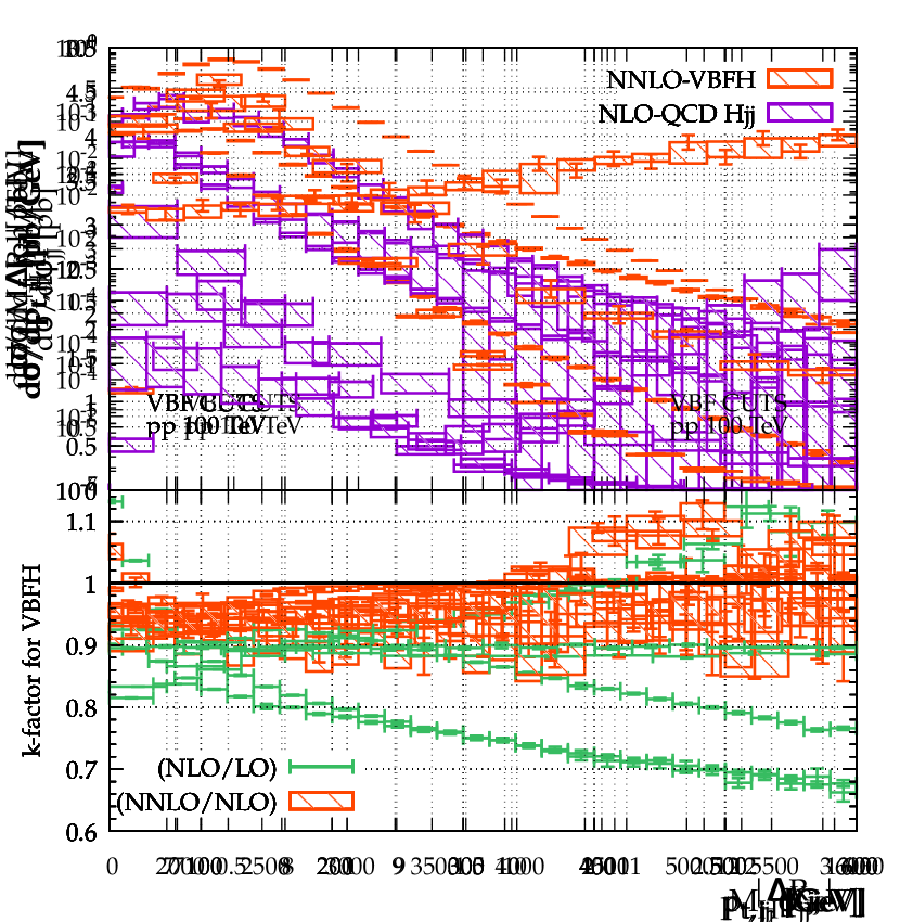
Figure 2.18: Similar to Figure 2.16. Left: Absolute value of the rapidity separation between the two leading jets. Right: Distance between the two leading jets in the rapidity-azimuthal plane.

Figure 2.19: Similar to Figure 2.16. Shown here is the azimuthal angle between the two leading jets.

2.3.2.6 Differential Distributions

In addition to the distributions already presented in the previous section, we here show a number of distributions to indicate the kinematical reach of the VBF channel at $100\;\mathrm{TeV}$. Assuming an integrated luminosity of $20$ ab^-1 we study how many events will be produced with a Higgs whose transverse momentum exceeds $p_{{t,\mathrm{min}}}$. In Figures 2.20 and 2.21 we show this distribution for various cut configurations. This variable is particularly interesting in the context of anomalous couplings in the weak sector. It can be seen that even under VBF cuts and requiring hard jets, a number of Higgs bosons with transverse momentum of the order $6\;\mathrm{TeV}$ will be produced in this scenario.

In Figure 2.22 we show the same distribution but fully inclusively and at various perturbative orders. Also shown is the k-factor going from LO to NLO and from NLO to NNLO. The perturbative corrections to this variable are modest as it is not sensitive to real radiation at the inclusive level. After applying VBF cuts and jet cuts the low $p_{{\mathrm{T},H}}$-spectrum receives moderate corrections whereas the corrections at larger values of $p_{{\mathrm{T},H}}$ can become very large as indicated in Figure 2.17.

In Figure 2.23 we show how many events will be produced with a dijet invariant mass exceeding $M_{\mathrm{min}}$ at various cut configurations. Because the two hardest jets in the VBF event are typically the proton remnants the invariant dijet mass can become very large. As can be seen from the figure, even after applying VBF cuts and requiring very hard jets hundreds of events with an invariant dijet mass larger than $60\;\mathrm{TeV}$ is expected. This is of interest when probing for BSM physics at the very highest scales. It is also worth noticing that the tail of the distribution is almost unaffected by the VBF cuts, as the VBF cuts are optimised to favour high invariant dijet events.

Figure 2.20: The total number of VBF events produced with $p_{{t,H}}>p_{{t,\mathrm{min}}}$ at a $100\;\mathrm{TeV}$ collider with an integrated luminosity of $20\mbox{ ab}^{-1}$ under three different jet $p_{\mathrm{T}}$ cuts. Left panel: $p_{\mathrm{T},H}$ in the range $0-2\;\mathrm{TeV}$. Right panel: $p_{\mathrm{T},H}$ in the range $2-10\;\mathrm{TeV}$.

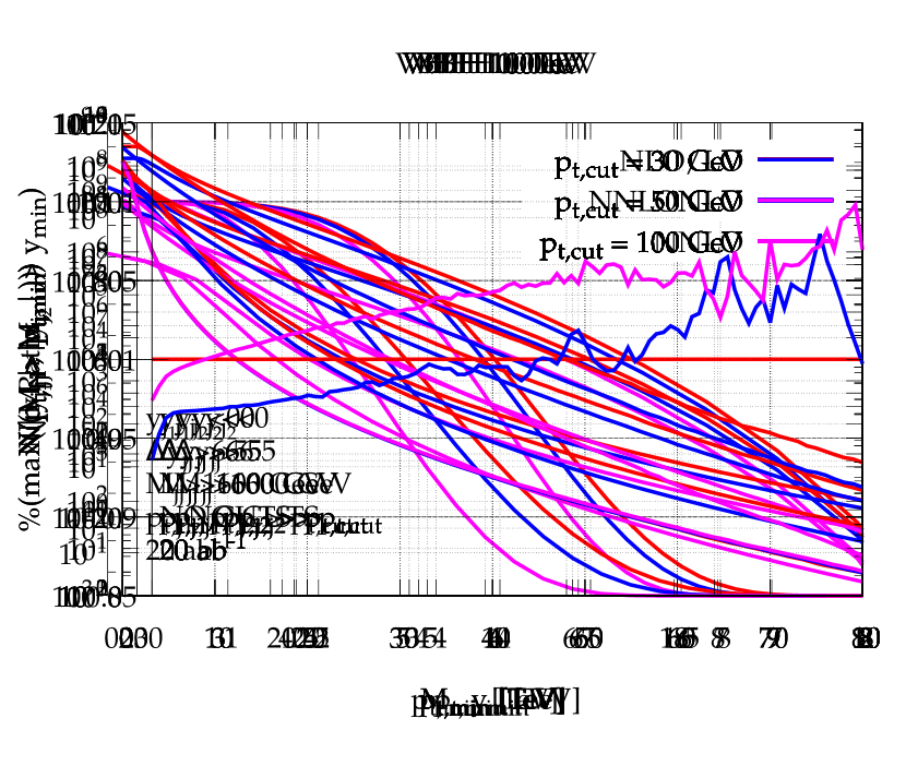
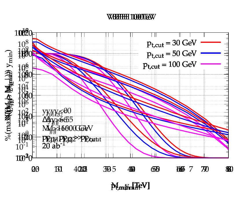
Figure 2.21: The total number of VBF events produced with $p_{{t,H}}>p_{{t,\mathrm{min}}}$ at a $100\;\mathrm{TeV}$ collider with an integrated luminosity of $20\mbox{ ab}^{-1}$under three different jet $p_{\mathrm{T}}$ cuts and with the VBF cuts of Equation 2.24 applied. Left panel: $p_{\mathrm{T},H}$ in the range $0-2\;\mathrm{TeV}$. Right panel: $p_{\mathrm{T},H}$ in the range $2-10\;\mathrm{TeV}$.

Figure 2.22: The total number of VBF events produced with $p_{{t,H}}>p_{{t,\mathrm{min}}}$ at a $100\;\mathrm{TeV}$ collider with an integrated luminosity of $20\mbox{ ab}^{-1}$ with no cuts applied. Left panel: Spectrum computed at LO, NLO and NNLO in QCD. Due to the small corrections the difference between the three curves is hard to see by eye. Right panel: The k-factor going from LO to NLO and NLO to NNLO.

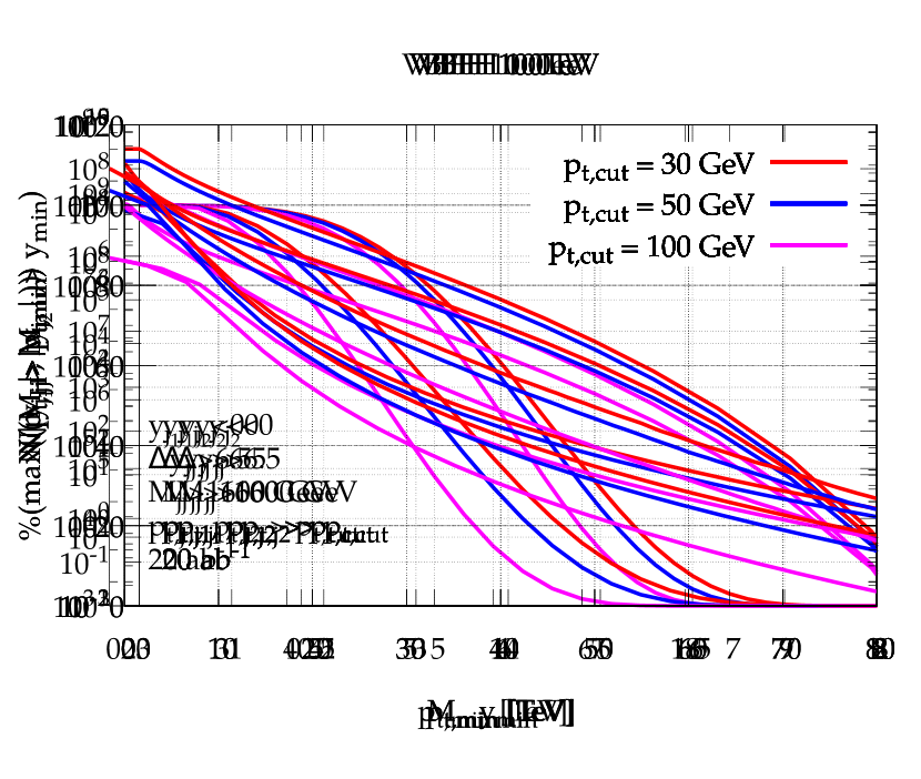
Figure 2.23: The total number of VBF events produced with $M_{j_{1}j_{2}}>M_{\mathrm{min}}$ at a $100\;\mathrm{TeV}$ collider with an integrated luminosity of $20\mbox{ ab}^{-1}$. Left panel: Three different jet $p_{\mathrm{T}}$ cuts applied but no VBF cuts applied. Right panel: VBF cuts of Equation 2.24 and three different jet $p_{\mathrm{T}}$ cuts applied.

2.3.2.7 Detector Implications

The requirement that the two hardest jets are in opposite detector hemispheres and are separated by at least $6.5$ units of rapidity, means that a symmetric detector in the style of ATLAS or CMS must have a rapidity reach well above $3.25$. In fact, looking at Figure 2.24, which shows the fraction of events which satisfy $\mathrm{max}(|y_{j_{1}}|,|y_{j_{2}}|)>y_{\mathrm{min}}$ for various cut configurations, it becomes clear that a detector with a rapidity reach of $4.5$ would at best only retain $40\%$ of the VBF events after VBF cuts are applied. Since a jet with $p_{\mathrm{T}}=30$ GeV can be produced at a rapidity of $\sim 8$ whereas a jet with $p_{\mathrm{T}}=100$ GeV can only be produced with rapidities up to $\sim 6.8$, the required rapidity reach of the detector will also depend on how well soft jets can be measured and controlled at $100\;\mathrm{TeV}$. In all cases a rapidity reach above 6 seems to be desirable.

Figure 2.24: The total fraction of events where $\mathrm{max}(|y_{j_{1}}|,|y_{j_{2}}|)>y_{\mathrm{min}}$ at a $100\;\mathrm{TeV}$ collider. Left panel: Three different jet $p_{\mathrm{T}}$ cuts applied but no VBF cuts applied. Right panel: VBF cuts of Equation 2.24 and three different jet $p_{\mathrm{T}}$ cuts applied.

2.4 Conclusions

With the calculation presented in this chapter, differential VBF Higgs production has been brought to the same NNLO level of accuracy that has been available for some time now for the ggH [110, 111] and VH [112] production channels. This constitutes the first fully differential NNLO $2\to 3$ hadron-collider calculation, an advance made possible thanks to the factorisable nature of the process. At both $13\;\mathrm{TeV}$ and $100\;\mathrm{TeV}$ the differential NNLO corrections are non-negligible, $5$–$10\%$, i.e. an order of magnitude larger than the corrections to the inclusive cross section. These corrections are found to be of the same order of magnitude as the NLO-EW corrections. Their size might even motivate a calculation one order higher, to N³LO, which we believe is within reach with the new “projection-to-Born” approach introduced here. It would also be of interest to obtain NNLO plus parton shower predictions, again matching the accuracy achieved recently in ggH [113, 114]. Our studies of VBF at a $100\;\mathrm{TeV}$ collider showed that it is still possible to suppress QCD backgrounds with suitable VBF cuts. However this suppression is roughly a factor two worse than what can be obtained at a $14\;\mathrm{TeV}$ collider. In addition to that, we found that experimental detectors with a rapidity reach in excess of $6$ is needed to catch all of the VBF signal.

Part II Parton Shower Matching

Chapter 3 The POWHEG Method

In this chapter we discuss how one might go about matching a fixed-order NLO calculation to a parton shower (NLOPS). The reason such a matching is desirable is obvious. Fixed-order calculations are very good at predicting observables that are inclusive over QCD radiation, but can never make accurate predictions for exclusive final states, due to the presence of soft and collinear divergences in the fixed order results. On the other hand Shower Monte Carlo programs can readily predict exclusive quantities through all order resummations, currently done in the leading logarithmic approximation. The showers are however limited to LO hard matrix elements at best, which do not reproduce inclusive quantities with the desired accuracy. A matching of the two approaches eliminate the deficiencies of both, retaining NLO accuracy of inclusive observables and exclusive final state generation.

Currently there exists two widely used methods for obtaining NLOPS accurate predictions: the MC@NLO method [79] and the POWHEG method [73, 86]. Here we spend some time reviewing the core results of the latter. In addition to that, a number of lesser used prescriptions exist [115, 116, 117, 118, 119, 120, 121, 122, 123], some because they are relatively recent additions and others because development halted after the initial ideas were presented. The POWHEG method has been implemented in two publicly available frameworks: Sherpa [92] and the POWHEG-BOX [74].

3.1 Matching NLO Calculations and Showers

Deriving all the details of the POWHEG method from first principles is a rather involved affair. Here we will assume that the reader already has familiarity with Shower Monte Carlos and only focus on the ingredients which are particular to the POWHEG method. The discussion below is therefore schematic at best. For a thorough discussion we refer the reader to [124, 125, 73, 86].

3.1.1 The Shower

Figure 3.1: Illustration of a final state parton of energy $E$ splitting into two partons with energy fraction $z$ and $1-z$ respectively.

To set up the notation we start by briefly considering a splitting of an incoming parton with energy $E$ into two partons with momentum fraction $z$ and $1-z$ respectively as shown in Figure 3.1. By momentum conservation the transverse momentum of the two outgoing partons with respect to the incoming parton will be

$$p_{\scriptscriptstyle\mathrm{T}}=\sin{\theta_{1}}zE=\sin{\theta_{2}}(1-z)E.$$ (3.1)

In the small angle approximation we have $\sin\theta\sim\theta$ from which it follows that

$$\theta=\frac{\theta_{1}}{1-z}=\frac{\theta_{2}}{z}.$$ (3.2)

Defining $t=E^{2}\theta^{2}$ we have

$$p_{\scriptscriptstyle\mathrm{T}}=\sqrt{t}z(1-z),$$ (3.3)

and one can then show that the probability for a parton with ordering parameter $t<t_{I}$ splitting into two partons with momentum fractions $z$ and $1-z$ is [124]

$$dP=F(z,t)dz\,dt\Delta_{s}(t_{I},t)=\frac{\alpha_{s}(p_{\scriptscriptstyle\mathrm{T}})}{2\pi}\hat{P}_{ab}(z)\frac{dt}{t}dz\Delta_{s}(t_{I},t).$$ (3.4)

Here $\hat{P}_{ab}$ are the unregularised Altarelli-Parisi splitting functions. They are intricately related to the splitting kernels of Equation 1.30. To lowest order they are given by [27]

$$\hat{P}_{gg}(z) =C_{A}\left[\frac{1-z}{z}+\frac{z}{1-z}+z(z-1)\right]\,,$$

$$\hat{P}_{qg}(z) =T_{R}\left[z^{2}+(1-z)^{2}\right]\,,$$

$$\hat{P}_{gq}(z) =C_{F}\left[\frac{1+(1-z)^{2}}{z}\right]\,,$$

$$\hat{P}_{qq}(z) =C_{F}\left[\frac{1+z^{2}}{1-z}\right]\,,$$ (3.5)

where $C_{F}=4/3$, $C_{A}=3$ and $T_{R}=1/2$. The Sudakov form factor, $\Delta_{s}$, is the probability that no branching has taken place between $t_{I}$ and $t$. Taking this as our ansatz we may now integrate Equation 3.4 and obtain

$$P(t,t_{0}) =\int_{t_{0}}^{t}{F(z,t^{\prime})dz\,dt^{\prime}\Delta_{s}(t_{I},t^{\prime})}\quad\Rightarrow\quad$$

$$\Delta_{s}(t,t_{0})=1-P(t,t_{0})=1-\int_{t_{0}}^{t}{F(z,t^{\prime})dz\,dt^{\prime}\Delta_{s}(t_{I},t^{\prime})},$$ (3.6)

which has the solution

$$\Delta_{s}(t,t_{0})=e^{-\int_{t_{0}}^{t}{F(z,t^{\prime})dz\,dt^{\prime}}}.$$ (3.7)

$t_{0}$ is a lower cut-off to avoid the pole in $\alpha_{s}$. It is typically of the order $1\;\mathrm{GeV}^{2}$. The angular ordered shower can now formally be expressed as the following recursive equation

$$\mathbb{S}(t_{I})=\Delta_{s}(t_{I},t_{0})\mathinner{\langle{\mathbb{I}}|}+\int_{t_{0}}^{t_{I}}{\Delta_{s}(t_{I},t)F(z,t)\mathbb{S}(z^{2}t)\mathbb{S}((1-z)^{2}t)dt\,dz},$$ (3.8)

where $\mathinner{\langle{\mathbb{I}}|}$ is the initial state parton. This equation can be solved iteratively through ordinary Monte Carlo methods, i.e. one generates a random number $r$ in the range $0$ to $1$ and solves $\Delta_{s}(t_{I},t)=r$ to find $t$. Then $z$ can be generated according to $F(z,t)$ and one repeats the procedure until $t<t_{0}$, at which point there can be no more emissions and the shower terminates. At leading-order it is straightforward to match the shower to a matrix element. If $d\sigma_{B}=|\mathcal{M_{B}}|^{2}d\Phi_{B}$ is the Born-level cross section, we simply act with $\mathbb{S}$ on $d\sigma_{B}$

$$d\sigma_{SMC}=d\sigma_{B}\big{\{}\Delta_{s}(t_{I},t_{0}) +\Delta_{s}(t_{I},t)F(z,t)dt\,dz$$

$$\times\left\{\Delta_{s}(t,t_{0})+\Delta_{s}(t,t^{\prime})F(z^{\prime},t^{\prime})dt^{\prime}\,dz^{\prime}\left\{\dots\right\}\right\}\big{\}}.$$ (3.9)

In this case the starting scale of the shower, $t_{I}$, should be set to the scale of the hard process, such that the parton shower correctly simulates soft and collinear partons while the matrix element describes the hard partons.

In order to discuss the POWHEG method we need to transform the above shower into a $p_{\scriptscriptstyle\mathrm{T}}$ ordered shower, that is we want to make sure that the hardest emission is generated first such that it can be described by the real matrix element. It is clear from Equation 3.3 that if one generates first an emission with $z\sim 1$ and then on the hardest emission line one generates an emission with $z^{\prime}\sim 1/2$ the $p_{\scriptscriptstyle\mathrm{T}}$ of the second emission can easily be larger than that of the first. We will state without proof than one can implement a $p_{\scriptscriptstyle\mathrm{T}}$ veto by modifying the Sudakov form factor in the obvious way

$$\ln\Delta_{R}(t,p_{\scriptscriptstyle\mathrm{T}})=-\int_{t_{0}}^{t}{dt^{\prime}}\int{dz\,F(z,t^{\prime})\theta(z(1-z)\sqrt{t^{\prime}}-p_{\scriptscriptstyle\mathrm{T}})}.$$ (3.10)

Using Equation 3.3 we can immediately transform this into an integral in $p_{\scriptscriptstyle\mathrm{T}}$. For the first emission the Sudakov form factor is then given by

$$\ln\Delta_{R}(t_{I},p_{\scriptscriptstyle\mathrm{T}})=-\int_{p_{\scriptscriptstyle\mathrm{T}}}^{\sqrt{t_{I}}/4}{2\,dp^{\prime}_{\scriptscriptstyle\mathrm{T}}}\int{dz^{\prime}\,F(z^{\prime},p^{\prime}_{\scriptscriptstyle\mathrm{T}})\theta(t_{I}-t^{\prime})}.$$ (3.11)

The differential cross section for the first emission can then be written

$$d\sigma=d\sigma_{B}\left\{\Delta_{R}(t_{I},p_{\scriptscriptstyle\mathrm{T}})+\Delta_{R}(t_{I},p_{\scriptscriptstyle\mathrm{T}})F(z,t)\theta(t_{I}-t)dt\,dz\right\},$$ (3.12)

which has the following $\mathcal{O}(\alpha_{s})$ expansion

$$d\sigma=d\sigma_{B}\left\{1-\int_{t_{0}}^{t_{I}}{dt^{\prime}}\int{dz\,F(z,t^{\prime})}+F(z,t)\theta(t_{I}-t)dt\,dz+\mathcal{O}(\alpha_{s}^{2})\right\}.$$ (3.13)

In order to turn this expression into something with which we can easily compare later on, we introduce the “+”-prescription to regulate the singularities in the splitting kernel. We define it in the following way

$$f(z)_{+}=f(z)-\delta(1-z)\int_{0}^{1}f(x)dx\,.$$ (3.14)

Doing so the above equation reduces to

$$d\sigma=d\sigma_{B}\left\{1+F(z,t)_{+}\theta(t_{I}-t)dt\,dz+\mathcal{O}(\alpha_{s}^{2})\right\}.$$ (3.15)

In writing the cross section in this form we have isolated the approximate Shower Monte Carlo NLO contribution. In fact, the two non-trivial terms of the bracket of Equation 3.13 correspond to the approximate virtual and real contributions to the cross section. The “+” prescriptions simply guarantees that the virtual and real singularities cancel. With this observation it becomes clear why matching fixed-order NLO calculations and partons showers poses a problem. If we are not careful the shower can generate configurations which are formally $\mathcal{O}(\alpha_{s})$ spoiling the claimed NLO accuracy. We can avoid this double counting by generating the first emission according to the NLO matrix element and all subsequent emissions with the shower.

3.1.2 POWHEG

Up until this point we have restricted our discussion to the effect of a parton shower on one jet only. In general we are interested in studying $2\,\rightarrow\,n$ scattering in which $m$ of the $n$ final states are coloured. In this case the above discussion is modified in the following way

• $F(z,t)\theta(t_{I}-t)dt\,dz$ is replaced by

  $$\sum_{i=1}^{m}F_{i}(z,t)\theta(t^{i}_{I}-t)dt\,dz,$$ (3.16)

  and we define

  $$\Delta_{R}(\{t_{I}\},p_{\scriptscriptstyle\mathrm{T}})=\prod_{i=1}^{m}\Delta^{i}_{R}(t^{i}_{I},p_{\scriptscriptstyle\mathrm{T}}).$$ (3.17)

  This in turn means that all lines, and not just the line emitting, will have $\Delta_{R}(t^{i}_{I},p_{\scriptscriptstyle\mathrm{T}})$ factors associated to them. These factors are there to ensure consistency with the $p_{\scriptscriptstyle\mathrm{T}}$ veto applied in the shower.

• Then one generates the hardest $p_{\scriptscriptstyle\mathrm{T}}$ according to $\Delta_{R}(\{t_{I}\},p_{\scriptscriptstyle\mathrm{T}})$ and chooses values $i$ and $z$ according to $F_{i}(z,t)\theta(t^{i}_{I}-t)$. From these two values we can construct the two new partons from $i$ and let the full $m+1$ partons shower with a $p_{\scriptscriptstyle\mathrm{T}}$ veto.

We now write the exact NLO formula for the cross section in the following schematic way

$$d\sigma^{\text{NLO}{}} =d\sigma^{\mathcal{B}}+d\sigma^{\mathcal{V}}+d\sigma^{\mathcal{R}}$$

$$=\mathcal{B}(\Phi_{\mathcal{B}})d\Phi_{\mathcal{B}}+\mathcal{V}(\Phi_{\mathcal{B}})d\Phi_{\mathcal{B}}+\left[\mathcal{R}(\Phi_{\mathcal{R}})d\Phi_{\mathcal{R}}-\mathcal{C}(\Phi_{\mathcal{R}})d\Phi_{\mathcal{R}}\mathbb{M}\right].$$ (3.18)

For simplicity we are assuming that the real matrix element, $\mathcal{R}$, has only one singular region, corresponding to the mapping $\mathbb{M}$ from the $m+1$-body kinematics to the $m$-body kinematics. Here we will assume the simplest case, which is that $\mathbb{M}\Phi_{\mathcal{R}}\rightarrow\Phi_{\mathcal{B}}$ and we write $d\Phi_{\mathcal{R}}=d\Phi_{\mathcal{B}}d\Phi_{r}$ where $d\Phi_{r}$ is the three dimensional phase space associated with the emitted parton. In this way we can rewrite the cross section in the following very suggestive way

$$d\sigma^{\text{NLO}{}} =\left[\mathcal{V}(\Phi_{\mathcal{B}})+\left(\mathcal{R}(\Phi_{\mathcal{R}})-\mathcal{C}(\Phi_{\mathcal{R}})\right)d\Phi_{r}\mathbb{M}\right]d\Phi_{\mathcal{B}}$$

$$\qquad+\left[\mathcal{B}(\Phi_{\mathcal{B}})-\mathcal{R}(\Phi_{\mathcal{R}})\Phi_{r}\mathbb{M}+\mathcal{R}(\Phi_{\mathcal{R}})\Phi_{r}\right]d\Phi_{\mathcal{B}}$$

$$=\left[\mathcal{V}(\Phi_{\mathcal{B}})+\left(\mathcal{R}(\Phi_{\mathcal{R}})-\mathcal{C}(\Phi_{\mathcal{R}})\right)d\Phi_{r}\mathbb{M}\right]d\Phi_{\mathcal{B}}$$

$$\qquad+\mathcal{B}(\Phi_{\mathcal{B}})\left[1+\frac{\mathcal{R}(\Phi_{\mathcal{R}})}{\mathcal{B}(\Phi_{\mathcal{B}})}(1-\mathbb{M})d\Phi_{r}\right]d\Phi_{\mathcal{B}}$$ (3.19)

By comparing the last line of this expression to the approximate NLO expression of Equation 3.15 we deduce how one would have to adjust Equation 3.12 in order to obtain the exact NLO expression. We first define the POWHEG Sudakov form factor by

$$\ln\bar{\Delta}(\Phi_{\mathcal{B}},p_{\scriptscriptstyle\mathrm{T}})=-\int{d\Phi_{r}\frac{\mathcal{R}(\Phi_{\mathcal{R}})}{\mathcal{B}(\Phi_{\mathcal{B}})}\theta(k_{\scriptscriptstyle\mathrm{T}}(\Phi_{\mathcal{R}})-p_{\scriptscriptstyle\mathrm{T}})}\,.$$ (3.20)

The function $k_{\scriptscriptstyle\mathrm{T}}(\Phi_{\mathcal{R}})$ is not unique, but has to correspond to the transverse momentum of the emitted parton relative to the emitter close to the singular limit. It is worth noticing, that in the collinear/soft limits this Sudakov form factor corresponds to the one of Equation 3.10 since in this limit the real matrix element factorises and $\mathcal{R}\sim\mathcal{B}\times F$. We then write the NLO cross section as

$$d\sigma^{\text{NLO}{}} =\left[\mathcal{V}(\Phi_{\mathcal{B}})+\left(\mathcal{R}(\Phi_{\mathcal{R}})-\mathcal{C}(\Phi_{\mathcal{R}})\right)d\Phi_{r}\mathbb{M}\right]d\Phi_{\mathcal{B}}$$

$$\qquad+\mathcal{B}(\Phi_{\mathcal{B}})d\Phi_{\mathcal{B}}\left[\bar{\Delta}(\Phi_{\mathcal{B}},0)+\bar{\Delta}(\Phi_{\mathcal{B}},p_{\scriptscriptstyle\mathrm{T}})\frac{\mathcal{R}(\Phi_{\mathcal{R}})}{\mathcal{B}(\Phi_{\mathcal{B}})}d\Phi_{r}\right].$$ (3.21)

By expanding $\bar{\Delta}$ in the above expression we exactly obtain Equation 3.19 analogously to the way Equation 3.15 can be obtained from Equation 3.12. One could in principle stop here and implement Equation 3.21 in a Shower Monte Carlo program. However, this expression has the disadvantage of being able to generate negative weights, simply because the first bracket is not required to be positive. A simple way of curing this problem is by introducing the NLO weighted Born term, $\bar{\mathcal{B}}$

$$\bar{\mathcal{B}}(\Phi_{\mathcal{B}})=\mathcal{B}(\Phi_{\mathcal{B}})+\mathcal{V}(\Phi_{\mathcal{B}})+\int{\left[\mathcal{R}(\Phi_{\mathcal{R}})-\mathcal{C}(\Phi_{\mathcal{R}})\right]d\Phi_{r}}$$ (3.22)

and write the hardest emission cross section as

$$d\sigma^{\text{NLO}{}}=\bar{\mathcal{B}}(\Phi_{\mathcal{B}})d\Phi_{\mathcal{B}}\left[\bar{\Delta}(\Phi_{\mathcal{B}},p_{\scriptscriptstyle\mathrm{T}}^{\mathrm{min}})+\bar{\Delta}(\Phi_{\mathcal{B}},k_{\scriptscriptstyle\mathrm{T}}(\Phi_{\mathcal{R}}))\frac{\mathcal{R}(\Phi_{\mathcal{R}})}{\mathcal{B}(\Phi_{\mathcal{B}})}d\Phi_{r}\right]$$ (3.23)

which is equivalent to Equation 3.21 at $\mathcal{O}(\alpha_{s})$. This expression avoids the generation of negative events, since the $\bar{\mathcal{B}}$ function is expected to be positive whenever perturbation theory is valid. Equation 3.23 is in essence the master formula of the POWHEG method. For the purpose of our discussion of MiNLO later on, we note that the $\bar{\mathcal{B}}$ function can receive corrections of $\mathcal{O}(\alpha_{s}^{2})$ without spoiling the accuracy of the cross section.

Before we continue and apply the POWHEG method to VBF $ZZjj$ production we will for completeness give the most general form of the above equation when there are more than just one singular region.

Equation 3.23 takes the following form [86]

$$d\sigma^{\texttt{POWHEG}{}} =\sum_{f_{b}}\bar{\mathcal{B}}^{f_{b}}(\Phi_{\mathcal{B}})d\Phi_{\mathcal{B}}\Big{[}\bar{\Delta}^{f_{b}}(\Phi_{\mathcal{B}},p_{\scriptscriptstyle\mathrm{T}}^{\mathrm{min}})$$

$$\qquad+\sum_{\alpha_{r}\in\{\alpha_{r}|f_{b}\}}\frac{\big{[}\bar{\Delta}^{f_{b}}(\Phi_{\mathcal{B}},k_{\scriptscriptstyle\mathrm{T}}(\Phi_{\mathcal{R}}))\theta(k_{\scriptscriptstyle\mathrm{T}}(\Phi_{\mathcal{R}}-p_{\scriptscriptstyle\mathrm{T}}^{\mathrm{min}}))\mathcal{R}(\Phi_{\mathcal{R}})d\Phi_{r}\big{]}^{\mathbb{M}^{\alpha_{r}}\Phi_{\mathcal{R}}=\Phi_{\mathcal{B}}}_{\alpha_{r}}}{\mathcal{B}(\Phi_{\mathcal{B}})}\Big{]}$$ (3.24)

where

$$\ln\bar{\Delta}^{f_{b}}(\Phi_{\mathcal{B}},p_{\scriptscriptstyle\mathrm{T}})=-\sum_{\alpha_{r}\in\{\alpha_{r}|f_{b}\}}\int{\frac{\big{[}\theta(k_{\scriptscriptstyle\mathrm{T}}(\Phi_{\mathcal{R}}-p_{\scriptscriptstyle\mathrm{T}}))\mathcal{R}(\Phi_{\mathcal{R}})d\Phi_{r}\big{]}^{\mathbb{M}^{\alpha_{r}}\Phi_{\mathcal{R}}=\Phi_{\mathcal{B}}}_{\alpha_{r}}}{\mathcal{B}(\Phi_{\mathcal{B}})}},$$ (3.25)

and

$$\bar{\mathcal{B}}^{f_{b}}(\Phi_{\mathcal{B}}) =\left[\mathcal{B}(\Phi_{\mathcal{B}})+\mathcal{V}(\Phi_{\mathcal{B}})\right]_{f_{b}}$$

$$\qquad+\sum_{\alpha_{r}\in\{\alpha_{r}|f_{b}\}}\int{\left[\left\{\mathcal{R}(\Phi_{\mathcal{R}})-\mathcal{C}(\Phi_{\mathcal{R}})\right\}d\Phi_{r}\right]_{\alpha_{r}}^{\mathbb{M}^{\alpha_{r}}\Phi_{\mathcal{R}}=\Phi_{\mathcal{B}}}}.$$ (3.26)

This expression looks complicated at first, but the various extra indices which have been introduced are easily explained. The outer sum runs over all Born-like flavour structures, $f_{b}$. To each such flavour structure exists a number of real graphs which have the underlying flavour structure, $f_{b}$. We label these real graphs by $\alpha_{r}$ according to their underlying flavour structure, $\alpha_{r}\in\{\alpha_{r}|f_{b}\}$, and such that they each have one and only one singular region. Hence

$$\mathcal{R}=\sum_{\alpha_{r}}\mathcal{R}^{\alpha_{r}}.$$ (3.27)

To each singular region corresponds a mapping, $\mathbb{M}^{\alpha_{r}}\Phi_{\mathcal{R}}\rightarrow\Phi_{\mathcal{B}}$ to a set of underlying Born-like momenta. Hence we see that Equation 3.24 simply sums over all possible Born-like flavour states while including all real contributions with that underlying flavour state.

It may so happen that certain real graphs have no singular regions and therefore no underlying Born structure. This happens for instance in Higgs production through gluon-fusion where the sub-process $q\bar{q}\rightarrow Hg$ can easily be seen to be non-singular. It can be useful to split the real contributions into the singular and non-singular ones to avoid the exponentiation of large corrections. In this case $\mathcal{R}$ should be substituted by the singular part of $\mathcal{R}$ and the non-singular part added outside of the $\bar{\mathcal{B}}$-function.

To construct the $\bar{\mathcal{B}}$ function it is convenient to introduce another function, $\tilde{\mathcal{B}}$, given by

$$\tilde{\mathcal{B}}^{f_{b}}(\Phi_{\mathcal{B}}) =\left[\mathcal{B}(\Phi_{\mathcal{B}})+\mathcal{V}(\Phi_{\mathcal{B}})\right]_{f_{b}}$$

$$\qquad+\sum_{\alpha_{r}\in\{\alpha_{r}|f_{b}\}}\left[\left\{\mathcal{R}(\Phi_{\mathcal{R}})-\mathcal{C}(\Phi_{\mathcal{R}})\right\}\left|\frac{\partial\Phi_{r}}{\partial X_{r}}\right|\right]_{\alpha_{r}}^{\mathbb{M}^{\alpha_{r}}\Phi_{\mathcal{R}}=\Phi_{\mathcal{B}}},$$ (3.28)

such that

$$\bar{\mathcal{B}}^{f_{b}}(\Phi_{\mathcal{B}})=\int_{0}^{1}dX_{r}^{(1)}\int_{0}^{1}dX_{r}^{(2)}\int_{0}^{1}dX_{r}^{(3)}\tilde{\mathcal{B}}^{f_{b}}(\Phi_{\mathcal{B}}).$$ (3.29)

Here $X_{r}=\{X_{r}^{(1)},X_{r}^{(2)},X_{r}^{(3)}\}$ is simply a parametrisation of the unit cube for the radiation variables.

Presently there exists a framework, the POWHEG-BOX [74], where a user may implement any fixed-order NLO calculation to be matched with the POWHEG method. The POWHEG method has been applied to a vast number of Standard Model processes and several studies of Beyond the Standard Model physics. The POWHEG-BOX requires the user to provide a list of Born, virtual, and real processes along with their respective matrix elements. The user also has to provide Born phase space mappings from the unit cube along with a suitable Jacobian. From these ingredients the POWHEG-BOX automatically finds the singular regions, constructs subtraction terms, and computes the $\bar{\mathcal{B}}$ and $\tilde{\mathcal{B}}$ functions. An interface to HERWIG and PYTHIA also exists, hence it is straightforward within this framework to match existing NLO fixed-order calculations to Shower Monte Carlo programs. In the next section we study the implementation of VBF $ZZjj$ production in the POWHEG-BOX.

3.2 Electroweak $ZZjj$ Production

A primary goal of the CERN Large Hadron Collider (LHC) is an in-depth understanding of the mechanism responsible for electroweak symmetry breaking. Data collected and analysed by the ATLAS [8] and CMS [9] collaborations have revealed the existence of a scalar boson with a mass of about $125\;\mathrm{GeV}$. Investigations on the properties of this new particle consolidate its interpretation as the Higgs boson of the Standard Model (SM). In particular, measurements of its spin and CP properties [126, 127, 128, 129, 130, 131, 132, 133] as well as of its couplings to gauge bosons and fermions so far have disclosed no deviation from the SM expectation of a spin-zero, CP-even particle. Should physics beyond the Standard Model be realised in nature, its effects on observables in the Higgs sector seem to be small, calling for high precision in experiment as well as in theoretical predictions.

An ideal environment for the determination of the tensor structure and strengths of the Higgs couplings to gauge bosons is provided by vector boson fusion processes [18, 134, 135]. As we have already seen in previous chapters, because of their very pronounced signature in phase space, featuring two well-separated jets in the forward regions of the detector, VBF reactions can be separated well from QCD-induced background reactions.

In this section we wish to present a tool for the simulation of $Z$-boson pair production via vector boson fusion. The purely electroweak process $pp\to ZZjj$ predominantly proceeds via the scattering of two quarks by the exchange of weak vector bosons in the $t$-channel with subsequent emission of two $Z$ bosons. Diagrams with a Higgs resonance contribute as well as weak boson scattering graphs that are sensitive to triple and quartic gauge boson couplings.

NLO-QCD corrections to this process, including leptonic decays of the $Z$ bosons in the $\ell^{+}\ell^{-}{\ell^{\prime}}^{+}{\ell^{\prime}}^{-}$ and $\ell^{+}\ell^{-}\nu\bar{\nu}$ modes, have been computed in Reference [136] and are publicly available in the computer package VBFNLO [137]. While that code allows the computation of, in principle, arbitrary distributions within experimentally feasible selection cuts, an interface to parton-shower Monte Carlo programs at NLO-QCD accuracy is not yet available. We have therefore worked out a matching of the NLO-QCD calculation with parton-shower programs in the framework of the POWHEG formalism described earlier in this chapter. To this end, we are making use of the POWHEG-BOX [74], a tool that provides all the process-independent building blocks of the matching procedure, but requires the user to implement process-specific ingredients in a specific format by themselves. Recently a Version 2 of the POWHEG-BOX has been released, POWHEG BOX V2. Version 2 includes a number of new features among which are

• the possibility to produce grids in parallel and combine them;

• the option to modify scales and parton distribution functions a posteriori, through a reweighting procedure of Les Houches events;

• a faster calculation of upper bounds, and the possibility to store upper bounds and combine them;

• an improvement in the separation of regions for the real radiation [138], which results in smoother distributions.

Given the complexity of electroweak $ZZjj$ production, we found it useful to take full advantage of these features and therefore implemented the process directly in Version 2 of the POWHEG-BOX.

In the following section we describe the technical details of our implementation. In Section 3.2.2 we present phenomenological results for some representative applications in the case of leptonic final states, in the case of cuts suitable to study the continuum, double-resonant production. We also discuss the potential of this process to constrain the size of dimension-six operators that arise in effective field theory approaches to physics beyond the Standard Model. In particular we study the capability of future Colliders to constrain the couplings even further.

3.2.1 Technical Details of the Implementation

Our implementation of electroweak $ZZjj$ production in the context of the POWHEG-BOX proceeds along the same lines as previous work done for $Zjj$ [139], $W^{+}W^{+}jj$ [140], and $W^{+}W^{-}jj$ production [141] via vector boson fusion. We therefore refrain from a detailed description of technical aspects that are common to all vector boson fusion processes considered so far, but refer the interested reader to the aforementioned references.

The first calculation of the NLO-QCD corrections to $ZZjj$ production via VBF in the context of the Standard Model, including decays of the $Z$-boson pair into four leptons or two leptons plus two neutrinos, has been presented in Reference [136] and is publicly available in the context of the VBFNLO package [137]. We adapted the matrix elements of that calculation to the format required by the POWHEG-BOX, and additionally computed the scattering amplitudes for the semi-leptonic decay modes of the $Z$ bosons, i.e. decay modes where one $Z$-boson decays leptonically and the other hadronically.

In addition to that we account for physics beyond the Standard Model in the weak gauge boson sector by means of an effective field theory approach [142] with operators of dimension six that affect triple and quartic gauge boson vertices, but do not change the QCD structure of the Standard Model. Details of the operators entering the Lagrangian are given later. Notice that because decays are not affected by QCD corrections, it is enough to have an LO implementation of the modified decay currents even at NLO in QCD. We could therefore adapt the LO implementation of the effective field theory in MadGraph 5 [143] for the modelling of the modified electroweak building blocks needed for $pp\to ZZjj$.

In either model, at order $\mathcal{O}(\alpha^{6})$ electroweak $ZZjj$ production predominantly proceeds via the scattering of two (anti-)quarks mediated by weak-boson exchange in the $t$-channel. The external $Z$ bosons that in turn decay into a pair of leptons, neutrinos, or quarks can be emitted from either of the two fermion lines, or stem from vector boson scattering sub-amplitudes of the type $VV\to VV$ (with $V$ generically denoting a photon, a $W^{\pm}$, or a $Z$ boson). In order to maintain electroweak gauge invariance, contributions with one or two photons instead of the $Z$ bosons and diagrams for single- and non-resonant four-fermion production in association with two jets have to be considered as well. A representative set of diagrams is depicted in Figure 3.2.

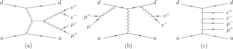
Figure 3.2: Representative Feynman diagrams for the partonic subprocess $ud\to e^{+}e^{-}\mu^{+}\mu^{-}ud$ at leading order.

For partonic subprocesses with quarks of identical flavour, in addition to the aforementioned $t$-channel exchange diagrams, $u$-channel diagrams arise that are taken fully into account. However, the interference of $u$-channel with $t$-channel contributions is neglected. We furthermore disregard contributions induced by the exchange of a weak boson in the $s$-channel. This gauge-invariant subset of diagrams is strongly suppressed in the phase-space regions that are explored experimentally in vector boson fusion searches, c.f. Reference [144] for a tree-level assessment of the numerical impact these contributions have in a realistic setup for the related case of electroweak $W^{+}W^{+}jj$ production at the LHC.

For $\ell^{+}\ell^{-}\nu_{\ell}\bar{\nu}_{\ell}$ final states we neglect the interference with $W^{+}W^{-}jj$ production, when the $W$ bosons decay into the same final state. In the case of QCD production, this interference has been shown to be very small [145]. In the semi-leptonic decay modes, interference effects between the scattering quarks and the decay quarks are neglected.

For simplicity, we will refer to the electroweak production processes $pp\to\ell^{+}\ell^{-}{\ell^{\prime}}^{+}{\ell^{\prime}}^{-}jj$, $pp\to\ell^{+}\ell^{-}\nu\bar{\nu}jj$, and $pp\to\ell^{+}\ell^{-}\bar{q}qjj$ within the aforementioned approximations as $ZZjj$ production via VBF in the fully leptonic, leptonic-invisible and semi-leptonic decay modes, respectively, even though we always include contributions from off-resonant diagrams that do not arise from a $ZZjj$ intermediate state.

In the case of semi-leptonic decay modes we do not explicitly take into account QCD corrections to the hadronic decays of the $Z$ bosons, or QCD corrections that connect the $ZZjj$ production with the $Z\to\bar{q}q$ decay processes. While the latter corrections are expected to be very small, corrections to the hadronic $Z$ decay are well-described by Monte-Carlo programs that are interfaced to our NLO-QCD calculation. In fact their decay machinery is tuned to reproduce collider data.

We note that, similarly to the cases of electroweak $Zjj$ and $W^{+}W^{-}jj$ production, the POWHEG-BOX requires a prescription for dealing with singularities emerging in the Born cross section for $pp\to ZZjj$ via VBF. One such type of singularities stems from collinear $q\to q\gamma$ configurations that emerge when a photon of low virtuality is exchanged in the $t$-channel. Phenomenologically, such contributions are irrelevant, as they are entirely removed once VBF-specific selection cuts are applied on the $ZZjj$ cross section that require the two partons of the underlying Born configuration to exhibit sufficient transverse momentum to be identified as tagging jets. We therefore drop this type of contributions already at generation level, by removing all events with an exchange boson in the $t$-channel with a virtuality smaller than $Q_{\mathrm{min}}^{2}=4\leavevmode\nobreak\ \mathrm{GeV}^{2}$. To improve the efficiency of the phase-space integration, we use a Born-suppression factor $F(\Phi_{n})$ that dampens the phase-space integrand whenever a singular configuration is approached [146]. This is ensured by the choice

$$F(\Phi_{n})=\left(\frac{p_{T,1}^{2}}{p_{T,1}^{2}+\Lambda^{2}}\right)^{2}\left(\frac{p_{T,2}^{2}}{p_{T,2}^{2}+\Lambda^{2}}\right)^{2}\,,$$ (3.30)

where the $p_{T,i}$ denote the transverse momenta of the two final-state partons of the underlying Born configuration, and $\Lambda$ is a cutoff parameter that we set to $10\;\mathrm{GeV}$.

In VBF $ZZjj$ production processes, an additional type of singular configurations is caused by diagrams with a quasi on-shell photon that decays into a fermion pair, $\gamma^{\star}\to f\bar{f}$. Such contributions can easily be identified by a small value of the invariant mass $m_{ff}$ of the decay system. In our simulations, we remove all configurations with $m_{ff}<m_{ff}^{\mathrm{gen}}$, where we set

$$m_{ff}^{\mathrm{gen}}=20\leavevmode\nobreak\ \mathrm{GeV}\,,$$ (3.31)

unless explicitly stated otherwise.

In the presence of a light Higgs boson, the VBF $ZZjj$ cross section receives contributions from two regions of phase space with very different kinematic properties. Therefore it is useful to split the phase space into two separate regions, around and away from the Higgs resonance. The full result is then obtained by adding the results of the two separate contributions [140].

3.2.2 Phenomenological Results

We will concentrate in the following on the fully charged leptonic decay mode, which has a smaller branching fraction than the semi-leptonic ($\ell^{+}\ell^{-}\bar{q}q$) or the leptonic-invisible ($\ell^{+}\ell^{-}\nu\bar{\nu}$) decay modes, but is experimentally cleaner. Because of the Higgs and $Z$ resonances, events tend to have either four leptons with an invariant mass close to the Higgs mass, or two pairs of leptons with an invariant mass close to the mass of the $Z$ boson each. Typically, according to whether one is interested in studying Higgs production with subsequent $H\to ZZ^{(\star)}$ decays or VBF $ZZjj$ production in the continuum one applies different invariant mass cuts that suppress one of the two contributions, and leave the other almost unchanged. Continuum VBF $ZZjj$ production is a rare SM process that is well-suited to probe triple but also quartic gauge boson couplings. In this section we present few sample results obtained with our POWHEG-BOX implementation, both in the pure SM and involving anomalous couplings that in our framework arise from an effective Lagrangian.

Let us stress here that the $\ell^{+}\ell^{-}\bar{q}q$ mode, although plagued by large QCD backgrounds, could in principle be studied with an analysis that uses boosted techniques and jet-substructure (see e.g. Reference [147]), along the lines of what was done in Reference [141]. However, because of the small production cross sections for VBF $ZZjj$, considering the boosted regime where only a tiny part of the inclusive cross section survives is pointless at the LHC.

3.2.2.1 Standard Model Results

With Run II already well under its way, and anticipating an energy upgrade of the LHC, we consider proton-proton collisions at a centre-of-mass energy of $\sqrt{s}=14\;\mathrm{TeV}$. We use the NLO-QCD set of the MSTW2008 parametrisation [148] for the parton distribution functions of the proton, as implemented in the LHAPDF library [149]. Jets are defined according to the anti-$k_{\scriptscriptstyle\mathrm{T}}$ algorithm [150, 75] with $R=0.4$, making use of the FASTJET package [76]. Electroweak input parameters are set according to known experimental values and tree-level electroweak relations. As input we use the mass of the $Z$ boson, $M_{\scriptscriptstyle\mathrm{Z}}=91.188\;\mathrm{GeV}$, the mass of the $W$ boson, $M_{\scriptscriptstyle\mathrm{W}}=80.419\;\mathrm{GeV}$, and the Fermi constant, $G_{F}=1.16639\times 10^{-5}\;\mathrm{GeV}^{-2}$. For the widths of the weak bosons we use $\Gamma_{Z}=2.51\;\mathrm{GeV}$ and $\Gamma_{W}=2.099\;\mathrm{GeV}$. The width of the Higgs boson is set to $\Gamma_{H}=0.00498\;\mathrm{GeV}$ which corresponds to $M_{\scriptscriptstyle\mathrm{H}}=125\;\mathrm{GeV}$. Factorisation and renormalisation scales are set to $\mu_{\mathrm{F}}=\mu_{\mathrm{R}}=M_{\scriptscriptstyle\mathrm{Z}}$ throughout, unless specified otherwise.

Here, we present numerical results for VBF $ZZjj$ production at the LHC in the fully leptonic decay mode. Our analysis requires each lepton pair to have an invariant mass close to $M_{\scriptscriptstyle\mathrm{Z}}$. This completely excludes any contamination from a Higgs boson consistent with the one observed by the ATLAS and CMS collaborations at $M_{\scriptscriptstyle\mathrm{H}}=125\;\mathrm{GeV}$ [8, 9], which results in $H\to ZZ^{(\star)}$ decays with at least one off-shell gauge boson. Our phenomenological study is inspired by [151]. In the following, we will always consider decays to $e^{+}e^{-}\mu^{+}\mu^{-}$. Neglecting same-type lepton interference effects, the cross-section for $Z$ bosons decaying to any combination of electrons and muons is twice as large. In Section 3.2.2.1 all results are quoted for the $pp\rightarrow e^{+}e^{-}\mu^{+}\mu^{-}jj$ decay mode only, whereas the results in Section 3.2.2.2 have been obtained for the $pp\rightarrow e^{+}e^{-}\mu^{+}\mu^{-}jj$ decay mode and then multiplied by two to account for any decay into electrons or muons, while neglecting same-type lepton interference effects.

The VBF and invariant mass cuts that we apply in the following, inspired by References [152, 153], are very effective in suppressing QCD-like processes with coloured objects in the $t$-channel. In particular, we require the presence of at least two jets with

$$p_{T,j}>25\leavevmode\nobreak\ \mathrm{GeV}\,,\quad y_{j}<4.5\,.$$ (3.32)

The two hardest jets satisfying these cuts are called “tagging jets” and are furthermore forced to be well separated by the VBF cuts

$$|y_{j_{1}}-y_{j_{2}}|>4.0\,,\quad y_{j_{1}}\cdot y_{j_{2}}<0\,,\quad m_{j_{1}j_{2}}>600\leavevmode\nobreak\ \mathrm{GeV}\,.$$ (3.33)

For the leptons we require

$$p_{T,\ell}>25\leavevmode\nobreak\ \mathrm{GeV}\,,\quad y_{\ell}<2.4\,,\quad R_{j\ell}>0.4\,.$$ (3.34)

In addition to that, we request that the leptons fall in between the two tagging jets

$$\mathrm{min}\{y_{j_{1}},y_{j_{2}}\}<y_{\ell}<\mathrm{max}\{y_{j_{1}},y_{j_{2}}\}\,.$$ (3.35)

Furthermore the two same-flavour opposite-charge leptons have to be close to the on-shell mass of the $Z$ boson,

$$66\leavevmode\nobreak\ \mathrm{GeV}<m_{\ell\ell}<116\leavevmode\nobreak\ \mathrm{GeV}\,.$$ (3.36)

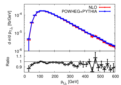
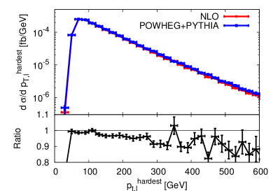
Figure 3.3: Transverse momentum distributions of the hardest jet (left) and the hardest lepton (right) for $pp\rightarrow e^{+}e^{-}\mu^{+}\mu^{-}jj$ at the LHC with $\sqrt{s}=14\leavevmode\nobreak\ \mathrm{TeV}$ within the cuts of Equations 3.32, 3.33, 3.34, 3.35 and 3.36 at NLO (red) and NLOPS (blue). The lower panel shows the ratio between NLO and NLOPS.

Because of the low mass of the Higgs boson and its very narrow width, this last cut ensures that contributions with an intermediate Higgs resonance are suppressed very strongly.

The inclusive cross section for VBF $e^{+}e^{-}\mu^{+}\mu^{-}jj$ production after applying the cuts of Equations 3.32, 3.33, 3.34, 3.35 and 3.36 is given by $\sigma_{ZZ}^{\mathrm{VBF}}=0.03003(7)\leavevmode\nobreak\ \mathrm{fb}$ at NLO in QCD and $\sigma_{ZZ}^{\mathrm{VBF}}=0.03249(4)\leavevmode\nobreak\ \mathrm{fb}$ at LO, where the uncertainties quoted are purely statistical. We then match the NLO calculation with the parton-shower program PYTHIA 6.4.25 [87] via POWHEG (NLOPS). The parton shower is run with the Perugia 0 tune, including hadronisation corrections, multi-parton interactions and underlying events. We do not take QED radiation effects into account. At the NLOPS level, we obtain an inclusive cross section of $\sigma_{ZZ}^{\mathrm{VBF}}=0.03084(7)\leavevmode\nobreak\ \mathrm{fb}$. In order to estimate the theoretical uncertainty of the calculation we have varied the renormalisation and factorisation scales in the range $M_{\scriptscriptstyle\mathrm{Z}}/2$ to $2M_{\scriptscriptstyle\mathrm{Z}}$, finding a change in the NLOPS cross section between $-0.0005\leavevmode\nobreak\ \mathrm{fb}$ and $+0.0001\leavevmode\nobreak\ \mathrm{fb}$ which is less than $3\%$.

Figure 3.3 shows the transverse momentum distributions of the hardest jet and the hardest lepton, respectively. The NLO and the NLOPS results agree very well for these two observables. In general, distributions involving leptons or any of the two hardest jets are only marginally distorted by the parton-shower. We notice only a small increase in the VBF cross section by $3\%$ when going from NLO to NLOPS. This is comparable to the size of the scale variation uncertainty.

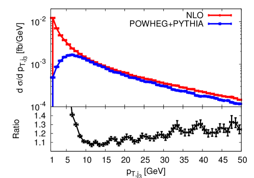
Figure 3.4: Transverse momentum distribution of the third jet for $pp\rightarrow e^{+}e^{-}\mu^{+}\mu^{-}jj$ at the LHC with $\sqrt{s}=14\leavevmode\nobreak\ \mathrm{TeV}$ within the cuts of Equations 3.32, 3.33, 3.34, 3.35 and 3.36, at NLO (red) and at NLOPS level (blue). The lower panel shows the ratio between NLO and NLOPS.

Illustrated in Figure 3.4 is the effect of the parton-shower on the transverse momentum of the third jet. In the NLO-QCD calculation for $pp\to ZZjj$ a third jet is described only at lowest non-vanishing order, as it solely arises via the real-emission contributions. When merged with the parton shower the soft-collinear radiation is resummed at leading-logarithmic accuracy via the Sudakov form factor, which results in the $p_{T,j_{3}}$ distribution being damped at low transverse momentum. At higher transverse momentum we observe that the parton shower tends to slightly soften the spectrum of the third jet. The parton shower also affects the rapidity of the third jet, giving rise to an increased central jet activity. This is expected since soft QCD radiation tends to populate the central region. In Figure 3.5 the rapidity of the third jet is shown with two different transverse-momentum cuts. Increasing the cut from $10\leavevmode\nobreak\ \mathrm{GeV}$ to $20\leavevmode\nobreak\ \mathrm{GeV}$ decreases the central jet activity of the parton shower without having any significant impact on the shape of the distribution at fixed order.

Instead of considering the absolute position of the third jet it can be useful to look at its relative position with respect to the two hardest jets. This is usually measured through the $y^{*}$ quantity,

$$y^{*}=y_{j_{3}}-\frac{y_{j_{1}}+y_{j_{2}}}{2}.$$ (3.37)

Figure 3.6 shows that the parton shower populates the region where $y^{*}$ is close to zero. This comes as no surprise, as we require the two hardest jets to be in opposite hemispheres and with a very large rapidity gap, and hence small values of $y^{*}$ will often coincide with a very central third jet. If we increase the cut on the transverse momentum of the third jet, we again see that the effect of the parton shower is minimised.

In fact, and not surprisingly, the parton-shower has very much the same impact on the distributions involving the third jet as was reported in [141] for VBF $W^{+}W^{-}jj$ .

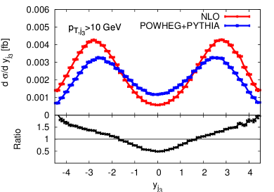
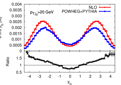
Figure 3.5: Rapidity of the third jet for $pp\rightarrow e^{+}e^{-}\mu^{+}\mu^{-}jj$ at the LHC with $\sqrt{s}=14\leavevmode\nobreak\ \mathrm{TeV}$ within the cuts of Equations 3.32, 3.33, 3.34, 3.35 and 3.36 and a transverse momentum cut on the third jet of $10\leavevmode\nobreak\ \mathrm{GeV}$ (left) and $20\leavevmode\nobreak\ \mathrm{GeV}$ (right), at NLO (red) and NLOPS (blue). The lower panel shows the ratio between NLO and NLOPS.

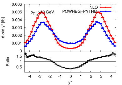
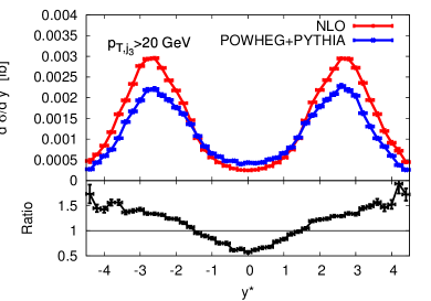
Figure 3.6: $y^{*}$ as defined in Equation 3.37 for $pp\rightarrow e^{+}e^{-}\mu^{+}\mu^{-}jj$ at the LHC with $\sqrt{s}=14\leavevmode\nobreak\ \mathrm{TeV}$ within the cuts of Equations 3.32, 3.33, 3.34, 3.35 and 3.36 and a transverse momentum cut on the third jet of $10\leavevmode\nobreak\ \mathrm{GeV}$ (left) and $20\leavevmode\nobreak\ \mathrm{GeV}$ (right), at NLO (red) and NLOPS (blue). The lower panel shows the ratio between NLO and NLOPS.

3.2.2.2 Effective Theory Results

Vector boson scattering processes offer an excellent test bed for the electroweak sector at the $\;\mathrm{TeV}$ scale. A convenient way to parametrise deviations from the Standard Model is through anomalous couplings or, alternatively, an effective field theory expansion. Such an effective theory is constructed as the low-energy approximation of a more fundamental theory, and is valid up to an energy scale $\Lambda$. The explicit dependence of predictions on the scale $\Lambda$ can be used to put limits on the scale of new physics itself. For scales $\Lambda$ much larger than the electroweak scale we can restrict ourselves to the first correction to the SM contributions with operators of dimension six.

The Lagrangian of the effective field theory can be written in the form [142]

$$\mathcal{L}_{\mathrm{eff}}=\sum_{i,d}{\frac{c_{i}^{(d)}}{\Lambda^{d-4}}\,\mathcal{O}_{i}^{(d)}}=\mathcal{L}_{\mathrm{SM}}+\sum_{i}{\frac{c_{i}^{(6)}}{\Lambda^{2}}\,\mathcal{O}_{i}^{(6)}}+\ldots\,,$$ (3.38)

where $d$ is the dimension of the operators $\mathcal{O}_{i}^{(d)}$, and the $c_{i}^{(d)}$ denote the coefficients of the expansion. For ease of notation we therefore drop the superscript $d=6$ in the following.

For our analysis of VBF $ZZjj$ production we include the three CP-conserving dimension-six operators [154, 142, 155],

$$\mathcal{O}_{WWW} =\mathrm{Tr}[W_{\mu\nu}W^{\nu\rho}W_{\rho}^{\mu}]\,,$$ (3.39)

$$\mathcal{O}_{W} =(D_{\mu}\Phi)^{\dagger}W^{\mu\nu}(D_{\nu}\Phi)\,,$$ (3.40)

$$\mathcal{O}_{B} =(D_{\mu}\Phi)^{\dagger}B^{\mu\nu}(D_{\nu}\Phi)\,,$$ (3.41)

and the two CP-violating operators ,

$$\mathcal{O}_{\tilde{W}WW} =\mathrm{Tr}[\tilde{W}_{\mu\nu}W^{\nu\rho}W_{\rho}^{\mu}]\,,$$ (3.42)

$$\mathcal{O}_{\tilde{W}} =(D_{\mu}\Phi)^{\dagger}\tilde{W}^{\mu\nu}(D_{\nu}\Phi)\,,$$ (3.43)

where $\Phi$ is the Higgs doublet field, and

$$D_{\mu} =\partial_{\mu}+\frac{i}{2}g\tau^{I}W_{\mu}^{I}+\frac{i}{2}g^{\prime}B_{\mu}\,,$$ (3.44)

$$W_{\mu\nu} =\frac{i}{2}g\tau^{I}(\partial_{\mu}W^{I}_{\nu}-\partial_{\nu}W^{I}_{\mu}+g\epsilon_{IJK}W^{J}_{\mu}W^{K}_{\nu})\,,$$ (3.45)

$$B_{\mu\nu} =\frac{i}{2}g^{\prime}(\partial_{\mu}B_{\nu}-\partial_{\nu}B_{\mu})\,.$$ (3.46)

Here, the $B^{\mu}$ and $W^{\mu}$ denote the $U(1)$ and $SU(2)$ gauge fields with the associated couplings $g^{\prime}$ and $g$, respectively, and $\tau^{I}$ the weak isospin matrices. The dual field strength tensor is defined as

$$\tilde{W}_{\mu\nu}=\epsilon_{\alpha\beta\mu\nu}W^{\alpha\beta}.$$ (3.47)

It is worth noting that the five operators of Equations 3.39, 3.40, 3.41, 3.42 and 3.43 form a minimal set of operators affecting the triple and quartic gauge boson couplings. For completeness we show which weak gauge boson vertices are affected by the five operators defined above in Table 3.1.

Our implementation of the effective Lagrangian approach for VBF $ZZjj$ production allows the user to specify the values of the $c_{i}/\Lambda^{2}$ coefficients in units of$\;\mathrm{TeV}^{-2}$ for each of the operators of Equations 3.39, 3.40, 3.41, 3.42 and 3.43. Here, we will show the effect of the two operators $\mathcal{O}_{WWW}$ and $\mathcal{O}_{\tilde{W}WW}$ for values of $c_{WWW}/\Lambda^{2}$ and $c_{\tilde{W}WW}/\Lambda^{2}$ consistent with current limits on the anomalous couplings $\lambda_{Z}$ and $\tilde{\lambda}_{Z}$. These can be transformed into limits on effective field theory parameters through a set of tree-level relations. However, the relations between the anomalous couplings and the effective field theory parameters are not exact, in the sense that they assume no form factor dependence and disregard contributions from higher dimensional operators.

	$WWZ$	$WW\gamma$	$WWH$	$ZZH$	$\gamma ZH$	$WWWW$	$WWZZ$	$WWZ\gamma$	$WW\gamma\gamma$
$\mathcal{O}_{WWW}$	x	x	-	-	-	x	x	x	x
$\mathcal{O}_{W}$	x	x	x	x	x	x	x	x	-
$\mathcal{O}_{B}$	x	x	-	x	x	-	-	-	-
$\mathcal{O}_{\tilde{W}WW}$	x	x	-	-	-	x	x	x	x
$\mathcal{O}_{\tilde{W}}$	x	x	x	x	x	-	-	-	-

Table 3.1: Crosses indicate triple and quartic weak boson vertices affected by the dimension-six operators of Equations 3.39, 3.40, 3.41, 3.42 and 3.43. Taken from Reference [155].

From [154, 156] we have

$$\frac{c_{WWW}}{\Lambda^{2}} =\frac{2}{3g^{2}M_{\scriptscriptstyle\mathrm{W}}^{2}}\lambda_{Z}\,,$$ (3.48)

$$\frac{c_{\tilde{W}WW}}{\Lambda^{2}} =\frac{1}{3g^{2}M_{\scriptscriptstyle\mathrm{W}}^{2}}\tilde{\lambda}_{Z}\,,$$ (3.49)

which translates into

$$-11.9\leavevmode\nobreak\ \mathrm{TeV}^{-2}< \frac{c_{WWW}}{\Lambda^{2}}<-1.94\leavevmode\nobreak\ \mathrm{TeV}^{-2}\,,$$ (3.50)

$$-19.4\leavevmode\nobreak\ \mathrm{TeV}^{-2}< \frac{c_{\tilde{W}WW}}{\Lambda^{2}}<-2.42\leavevmode\nobreak\ \mathrm{TeV}^{-2}\,,$$ (3.51)

when using the current combined limits of [157] at the $68\%$ confidence level. The limits become compatible with the Standard Model at the $95\%$ confidence level.

Our setup is identical to that of Section 3.2.2.1, except we choose running factorisation and renormalisation scales,

$$\mu_{R}=\mu_{F}={\frac{\sqrt{M_{\scriptscriptstyle\mathrm{Z}}^{2}+p_{T,Z_{1}}^{2}}+\sqrt{M_{\scriptscriptstyle\mathrm{Z}}^{2}+p_{T,Z_{2}}^{2}}+\sum_{i}{p_{T,i}}}{2}}\,,$$ (3.52)

where the $p_{T,i}$ are the transverse momenta of the (two or three) final state partons and the $p_{T,Z_{i}}$ the transverse momenta of a same-type lepton pair. Such a dynamical scale is expected to optimally account for the high-transverse momentum region where the effective operators have the largest impact.

Our analysis within the effective field theory approach is done in analogy to the SM analysis of Section 3.2.2.1. We present results obtained for the $\ell^{+}\ell^{-}{\ell^{\prime}}^{+}{\ell^{\prime}}^{-}$ decay mode within the cuts of Equations 3.32, 3.33, 3.34, 3.35 and 3.36. We account for decays into any combination of electrons and muons by multiplying results obtained for the $e^{+}e^{-}\mu^{+}\mu^{-}$ decay mode by a factor of two. As mentioned earlier this procedure neglects any interference effects for the leptons. In order to illustrate the effect dimension-six operators can have on observables we consider the operators $\mathcal{O}_{WWW}$ and $\mathcal{O}_{\tilde{W}WW}$ independently by setting the associated expansion coefficients to values compatible with the current experimental bounds of Equations 3.50 and 3.51, and all other to zero. To this end, we separately choose $c_{WWW}/\Lambda^{2}=-5\leavevmode\nobreak\ \mathrm{TeV}^{-2}$ and $c_{\tilde{W}WW}/\Lambda^{2}=-5\leavevmode\nobreak\ \mathrm{TeV}^{-2}$. In diagrams where more than one vertex could be affected by the effective operator, we only turn on the effective coupling for one vertex at a time. This is consistent with only considering dimension six operators, as diagrams suppressed by more than one factor of $\Lambda^{-2}$ should also receive corrections from operators of higher dimension. Because of the explicit scale suppression of the effective operators, it is expected that deviations from the Standard Model are most easily seen in the tails of differential distributions that are sensitive to the high-energy regime. From our SM analysis of Section 3.2.2.1 we may conclude that a parton shower has very little effect on the distributions that do not involve the third jet. In this section we therefore only discuss fixed-order results.

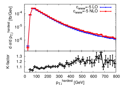
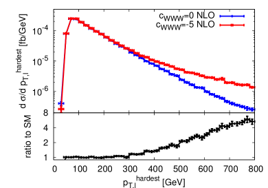
Figure 3.7: Transverse momentum distribution of the hardest lepton for $pp\rightarrow e^{+}e^{-}\mu^{+}\mu^{-}jj$ at the LHC with $\sqrt{s}=14\leavevmode\nobreak\ \mathrm{TeV}$ within the cuts of Equations 3.32, 3.33, 3.34, 3.35 and 3.36, with $c_{WWW}/\Lambda^{2}=-5\leavevmode\nobreak\ \mathrm{TeV}^{-2}$ at LO and NLO (left panel), and at NLO with $c_{WWW}/\Lambda^{2}=-5\leavevmode\nobreak\ \mathrm{TeV}^{-2}$ and $c_{WWW}/\Lambda^{2}=0$ (right panel). The lower panels show the respective ratios.

In Figure 3.7 (left panel) we show the transverse mass distribution of the hardest lepton at LO and NLO for $c_{WWW}/\Lambda^{2}=-5\leavevmode\nobreak\ \mathrm{TeV}^{-2}$ together with the associated dynamical $K$-factor, defined by

$$K(x)=\frac{d\sigma_{NLO}/dx}{d\sigma_{LO}/dx}\,,$$ (3.53)

and a comparison of the NLO prediction for $c_{WWW}/\Lambda^{2}=-5\leavevmode\nobreak\ \mathrm{TeV}^{-2}$ with the SM result (right panel). All other dimension-six operator coefficients are set to zero. We note that the impact of the NLO-QCD corrections and the considered dimension-six operator contributions are of the same order of magnitude in the range of low to intermediate transverse momenta. For smaller absolute values of $c_{WWW}/\Lambda^{2}$ the NLO corrections are significant up to even higher transverse momenta. Hence, in that case, in order to unambiguously distinguish new physics from higher-order perturbative effects in the Standard Model, full NLO-QCD results have to be considered.

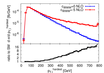
Figure 3.8: Transverse momentum distribution of the hardest lepton for $pp\rightarrow e^{+}e^{-}\mu^{+}\mu^{-}jj$ at the LHC with $\sqrt{s}=14\leavevmode\nobreak\ \mathrm{TeV}$ within the cuts of Equations 3.32, 3.33, 3.34, 3.35 and 3.36, at NLO with $c_{\tilde{W}WW}/\Lambda^{2}=-5\leavevmode\nobreak\ \mathrm{TeV}^{-2}$ and $c_{\tilde{W}WW}/\Lambda^{2}=0$, together with the respective ratio.

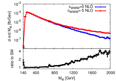
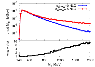
Figure 3.9: Invariant mass distribution of the four-lepton system in $pp\rightarrow e^{+}e^{-}\mu^{+}\mu^{-}jj$ at the LHC with $\sqrt{s}=14\leavevmode\nobreak\ \mathrm{TeV}$ within the cuts of Equations 3.32, 3.33, 3.34, 3.35 and 3.36, at NLO with $c_{WWW}/\Lambda^{2}=-5\leavevmode\nobreak\ \mathrm{TeV}^{-2}$ and $c_{WWW}/\Lambda^{2}=0$ (left panel), $c_{\tilde{W}WW}/\Lambda^{2}=-5\leavevmode\nobreak\ \mathrm{TeV}^{-2}$ and $c_{\tilde{W}WW}/\Lambda^{2}=0$ (right panel), together with the respective ratio.

When fixing $c_{WWW}=c_{\tilde{W}WW}$ one notices that the CP-violating operator $\mathcal{O}_{\tilde{W}WW}$ yields an enhancement in the tails of the transverse momentum distribution of the hardest lepton that is larger by roughly a factor two, cf. Figure 3.8. This is due to the normalisation chosen in Equation 3.47, which would be more naturally defined with a factor $1/2$ on the right-hand-side. Qualitatively similar results are obtained for the invariant mass of the four-lepton system, as illustrated by Figure 3.9.

In order to estimate how sensitive the LHC is to the two couplings $c_{WWW}/\Lambda^{2}$ and $c_{\tilde{W}WW}/\Lambda^{2}$ we have computed the number of events in the tail of the transverse momentum distribution of the hardest lepton, $p_{T,\ell}^{\mathrm{hardest}}>340\leavevmode\nobreak\ \mathrm{GeV}$, for the Standard Model, for $c_{WWW}/\Lambda^{2}=-5\leavevmode\nobreak\ \mathrm{TeV}^{-2}$ and for $c_{\tilde{W}WW}/\Lambda^{2}=-5\leavevmode\nobreak\ \mathrm{TeV}^{-2}$, respectively, with integrated luminosities of $300\leavevmode\nobreak\ \mathrm{fb}^{-1}$ and $3000\leavevmode\nobreak\ \mathrm{fb}^{-1}$, cf. Table 3.2. The cut-off value of $340\leavevmode\nobreak\ \mathrm{GeV}$ is chosen upon inspection of the transverse-momentum distributions, where we start observing a significant deviation from the Standard Model around this region, cf. Figures 3.7 and 3.8. We note that for different values of $c_{WWW}/\Lambda^{2}$ and $c_{\tilde{W}WW}/\Lambda^{2}$, we would find different values for the cut-off. For consistency we will use $p_{T,\ell}^{\mathrm{hardest}}=340\leavevmode\nobreak\ \mathrm{GeV}$ as cut-off for all values of $c_{WWW}/\Lambda^{2}$ and $c_{\tilde{W}WW}/\Lambda^{2}$.

	events @ $300\leavevmode\nobreak\ \mathrm{fb}^{-1}$	significance	events @ $3000\leavevmode\nobreak\ \mathrm{fb}^{-1}$	significance
SM	0.692	-	6.92	-
$\frac{c_{WWW}}{\Lambda^{2}}=-5\leavevmode\nobreak\ \mathrm{TeV}^{-2}$	1.49	0.96	14.9	3.0
$\frac{c_{\tilde{W}WW}}{\Lambda^{2}}=-5\leavevmode\nobreak\ \mathrm{TeV}^{-2}$	3.76	3.7	37.6	11.64

Table 3.2: Number of events for $pp\rightarrow\ell^{+}\ell^{-}{\ell^{\prime}}^{+}{\ell^{\prime}}^{-}jj$ at NLO-QCD at the LHC with $\sqrt{s}=14\leavevmode\nobreak\ \mathrm{TeV}$ within the cuts of Equations 3.32, 3.33, 3.34, 3.35 and 3.36 and an additional cut of $p_{T,\ell}^{\mathrm{hardest}}>340\leavevmode\nobreak\ \mathrm{GeV}$, together with the significance of the signal defined in Equation 3.54.

	events @ $300\leavevmode\nobreak\ \mathrm{fb}^{-1}$	significance	events @ $3000\leavevmode\nobreak\ \mathrm{fb}^{-1}$	significance
SM	0.599	-	5.99	-
$\frac{c_{WWW}}{\Lambda^{2}}=-5\leavevmode\nobreak\ \mathrm{TeV}^{-2}$	1.22	0.80	12.2	2.5
$\frac{c_{\tilde{W}WW}}{\Lambda^{2}}=-5\leavevmode\nobreak\ \mathrm{TeV}^{-2}$	3.03	3.1	30.3	9.9

Table 3.3: Same as Table 3.2, but at LO.

The significance of a non-Standard Model (nSM) signal is defined via the number of events in the nSM and the SM scenarios as

$$\frac{|\#\,\mathrm{events(nSM)}-\#\,\mathrm{events(SM)}|}{\sqrt{\#\,\mathrm{events(SM)}}}\,.$$ (3.54)

Assuming that events are distributed according to a Gaussian distribution, a one-, two- and three-sigma significance correspond to the well-known 68%, 95% and 99.8% probabilities. When the expected number of SM events is low, one needs however to bear in mind that events are distributed according to a Poisson distribution. In this case these significances correspond to lower probabilities. However, when the expected number of SM events is larger than five, we find that these probabilities differ already by 1%.

At $300\leavevmode\nobreak\ \mathrm{fb}^{-1}$ the dimension-six operators result in a significant signal for the CP-violating coupling. However, in the high-luminosity phase of the LHC with $3000\leavevmode\nobreak\ \mathrm{fb}^{-1}$, CP-conserving operators with $c_{WWW}/\Lambda^{2}=-5\leavevmode\nobreak\ \mathrm{TeV}^{-2}$ become significant at the three sigma level and CP-violating operators with $c_{\tilde{W}WW}/\Lambda^{2}=-5\leavevmode\nobreak\ \mathrm{TeV}^{-2}$ are significant to more than five sigma.

It is worth noting that the significance decreases, if only LO results are taken into account. Comparing Tables 3.2 and 3.3 we observe that the significance increases by $\sim 20\%$, when NLO-QCD corrections are included. This strongly favours including the NLO-QCD corrections, as a similar gain in significance by technical means would require an increase in luminosity of $\sim 44\%$.

$\frac{c_{WWW}}{\Lambda^{2}}$	events @ $14\leavevmode\nobreak\ \mathrm{TeV}$	significance	events @ $33\leavevmode\nobreak\ \mathrm{TeV}$	significance	events @ $100\leavevmode\nobreak\ \mathrm{TeV}$	significance
$0.0\leavevmode\nobreak\ \mathrm{TeV}^{-2}$	0.200	-	3.26	-	32.1	-
$-2.0\leavevmode\nobreak\ \mathrm{TeV}^{-2}$	0.234	0.0765	4.47	0.671	74.6	7.51
$-4.0\leavevmode\nobreak\ \mathrm{TeV}^{-2}$	0.334	0.301	8.12	2.70	203	30.2
$-6.0\leavevmode\nobreak\ \mathrm{TeV}^{-2}$	0.496	0.663	14.3	6.10	419	68.3
$-8.0\leavevmode\nobreak\ \mathrm{TeV}^{-2}$	0.725	1.18	22.8	10.8	720	122
$-10.0\leavevmode\nobreak\ \mathrm{TeV}^{-2}$	1.01	1.82	33.7	16.9	1110	190

Table 3.4: Number of events for $pp\rightarrow\ell^{+}\ell^{-}{\ell^{\prime}}^{+}{\ell^{\prime}}^{-}jj$ for different collider energies with an integrated luminosity $100\leavevmode\nobreak\ \mathrm{fb}^{-1}$, within the cuts of Equations 3.32, 3.33, 3.34, 3.35 and 3.36 and an additional cut of $p_{T,\ell}^{\mathrm{hardest}}>340\leavevmode\nobreak\ \mathrm{GeV}$ in the SM and including the effect of ${\mathcal{O}}_{WWW}$, together with the significance of the signal defined in Equation 3.54.

$\frac{c_{\tilde{W}WW}}{\Lambda^{2}}$	events @ $14\leavevmode\nobreak\ \mathrm{TeV}$	significance	events @ $33\leavevmode\nobreak\ \mathrm{TeV}$	significance	events @ $100\leavevmode\nobreak\ \mathrm{TeV}$	significance
$0.0\leavevmode\nobreak\ \mathrm{TeV}^{-2}$	0.200	-	3.26	-	32.1	-
$-2.0\leavevmode\nobreak\ \mathrm{TeV}^{-2}$	0.331	0.293	8.12	2.70	205	30.3
$-4.0\leavevmode\nobreak\ \mathrm{TeV}^{-2}$	0.717	1.16	22.8	10.9	723	121
$-6.0\leavevmode\nobreak\ \mathrm{TeV}^{-2}$	1.36	2.60	47.3	24.4	1580	272
$-8.0\leavevmode\nobreak\ \mathrm{TeV}^{-2}$	2.27	4.64	81.7	43.5	2790	484
$-10.0\leavevmode\nobreak\ \mathrm{TeV}^{-2}$	3.43	7.23	125	67.7	4350	759

Table 3.5: Same as Table 3.4, but including the operator ${\mathcal{O}}_{\tilde{W}WW}$.

If we consider only contributions of one operator, e.g. $\mathcal{O}_{WWW}$, the matrix element squared schematically takes the form

$$|\mathcal{M}|^{2}=|\mathcal{M}_{SM}|^{2}+\frac{c^{2}_{WWW}}{\Lambda^{4}}|\tilde{\mathcal{M}}_{WWW}|^{2}+\frac{c_{WWW}}{\Lambda^{2}}(\tilde{\mathcal{M}}_{WWW}\mathcal{M}^{*}_{SM}+\mathcal{M}_{SM}\tilde{\mathcal{M}}^{*}_{WWW})\,.$$ (3.55)

By calculating the cross section for at least three different values of the coupling $c_{WWW}/\Lambda^{2}$ (or $c_{\tilde{W}WW}/\Lambda^{2}$) it is possible to interpolate the cross section for any value of the coupling. Using this, we expect the following one sigma bounds for the LHC at $300\leavevmode\nobreak\ \mathrm{fb}^{-1}$,

$$-4.98\leavevmode\nobreak\ \mathrm{TeV}^{-2}< \frac{c_{WWW}}{\Lambda^{2}}<5.12\leavevmode\nobreak\ \mathrm{TeV}^{-2}\,,$$ (3.56)

$$-2.54\leavevmode\nobreak\ \mathrm{TeV}^{-2}< \frac{c_{\tilde{W}WW}}{\Lambda^{2}}<2.54\leavevmode\nobreak\ \mathrm{TeV}^{-2}\,,$$ (3.57)

and at $3000\leavevmode\nobreak\ \mathrm{fb}^{-1}$,

$$-2.77\leavevmode\nobreak\ \mathrm{TeV}^{-2}< \frac{c_{WWW}}{\Lambda^{2}}<2.91\leavevmode\nobreak\ \mathrm{TeV}^{-2}\,,$$ (3.58)

$$-1.43\leavevmode\nobreak\ \mathrm{TeV}^{-2}< \frac{c_{\tilde{W}WW}}{\Lambda^{2}}<1.43\leavevmode\nobreak\ \mathrm{TeV}^{-2}\,.$$ (3.59)

We see that these limits are already tighter than the current experimental limits quoted in Equations 3.50 and 3.51. Note that the limits only improve by a factor $10^{1/4}\sim 1.8$ when the luminosity is increased by a factor of $10$. This is related to the fact that for large values of $c_{WWW}/\Lambda^{2}$ we are essentially only probing $c^{2}_{WWW}/\Lambda^{4}$, see Equation 3.55. The limits on the coupling improve then with a quartic root of the available luminosity.

$$14\leavevmode\nobreak\ \mathrm{TeV}$$

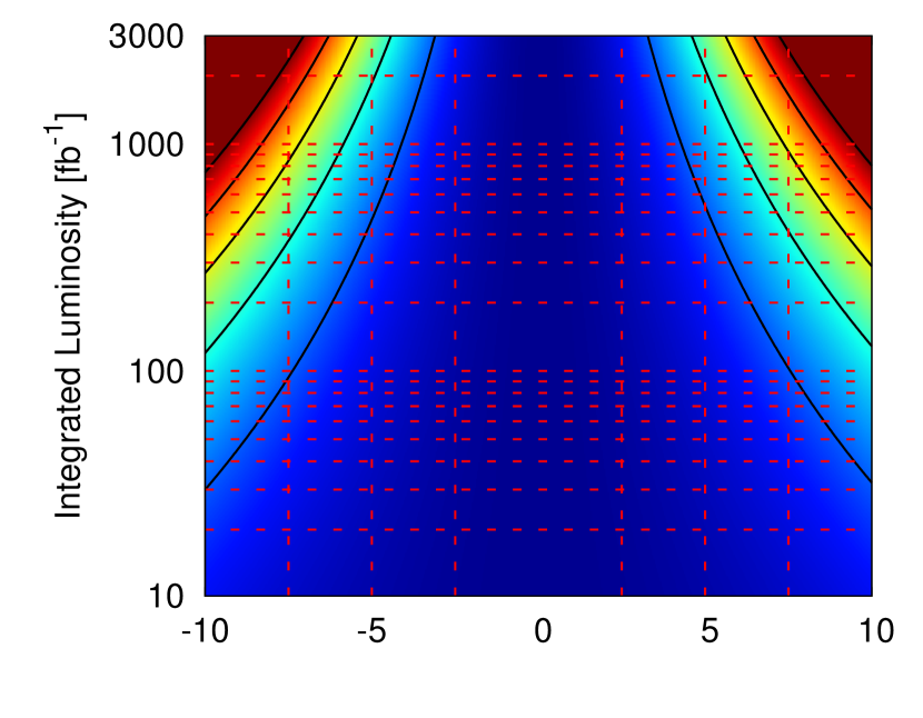
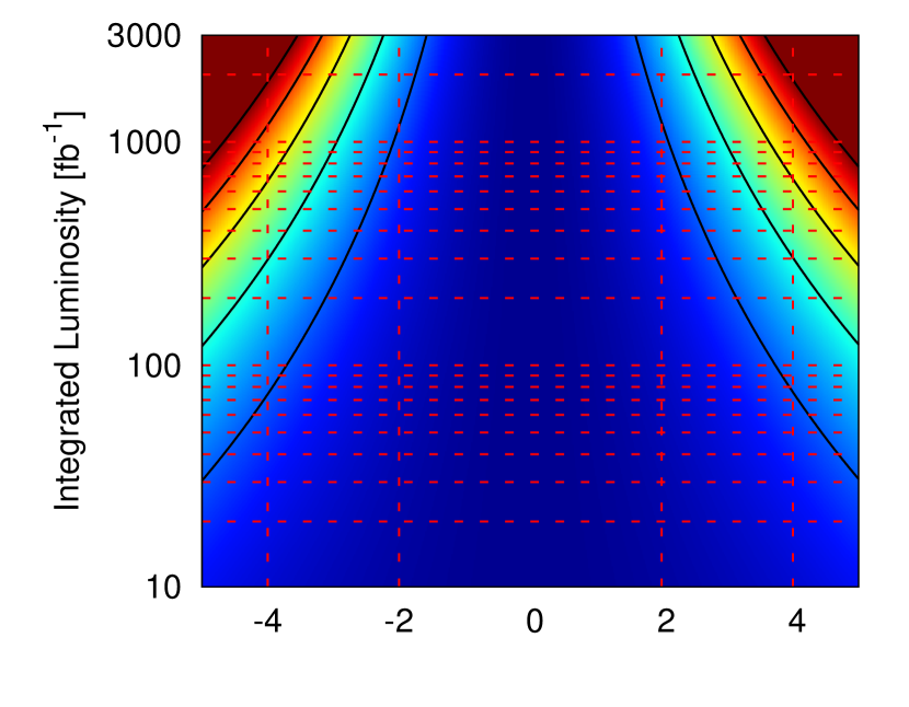
$$33\leavevmode\nobreak\ \mathrm{TeV}$$

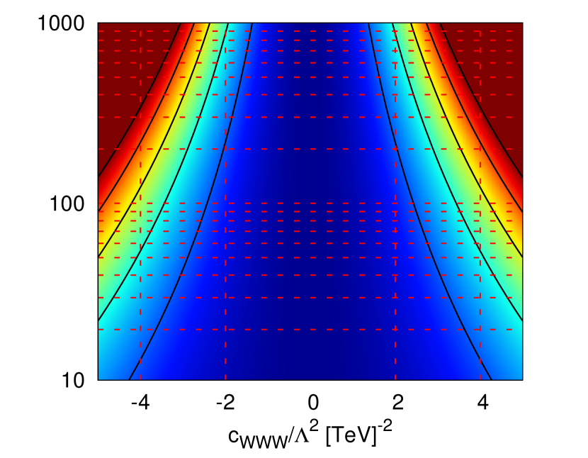
$$100\leavevmode\nobreak\ \mathrm{TeV}$$

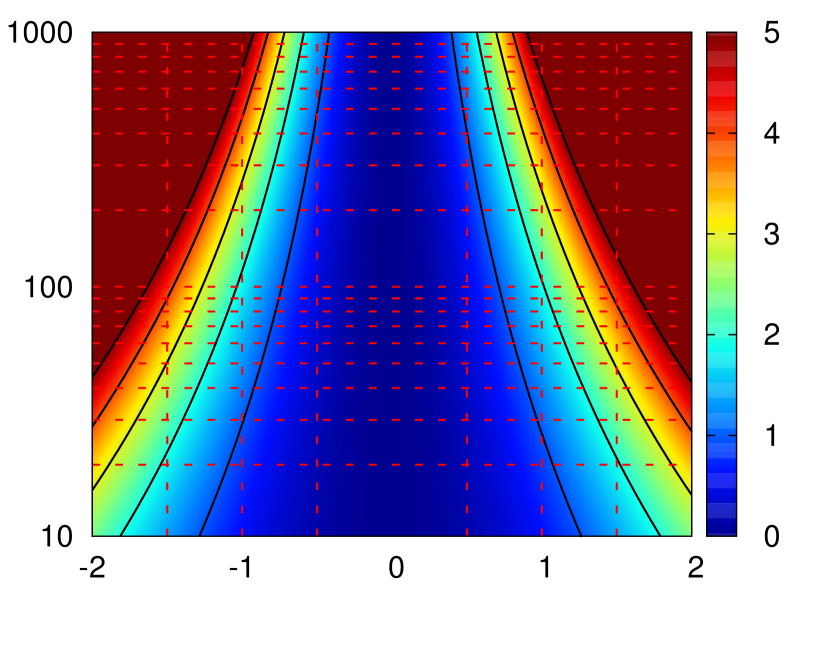
Figure 3.10: Significance of the two couplings $c_{WWW}/\Lambda^{2}$ and $c_{\tilde{W}WW}/\Lambda^{2}$ for the process $pp\rightarrow\ell^{+}\ell^{-}\ell^{\prime+}\ell^{\prime-}jj$ at $14\leavevmode\nobreak\ \mathrm{TeV}$, $33\leavevmode\nobreak\ \mathrm{TeV}$ and $100\leavevmode\nobreak\ \mathrm{TeV}$ within the cuts of Equations 3.32, 3.33, 3.34, 3.35 and 3.36 and $p_{T,\ell}^{\mathrm{hardest}}>340\leavevmode\nobreak\ \mathrm{GeV}$, as a function of the integrated luminosity. The five black lines indicate one, two, three, four and five sigma significance defined in Equation 3.54, corresponding to the colour code indicated on the right-hand-side.

Even better significances could be obtained with hadron colliders operating at higher energies, such as the high-energy upgrade of the LHC (HE-LHC) with an energy of $\sqrt{s}=33\;\mathrm{TeV}$, or a FCC with an energy of up to $\sqrt{s}=100\;\mathrm{TeV}$. Tables 3.4 and 3.5 show expected numbers of events and associated significances for various scenarios at the LHC, HE-LHC and FCC at LO. As reported above the significance is expected to increase at NLO QCD.

Depending on the luminosity delivered, already for rather small values of the operator coefficient $c_{WWW}/\Lambda^{2}$ an excess over the SM values should be visible. Here we observe that the significances grow faster than the collider energy squared.

To better illustrate the impact of increasing energy and integrated luminosity, we have plotted the significance of a signal as a function of the value of the coupling and the integrated luminosity for each of the energies $14\leavevmode\nobreak\ \mathrm{TeV}$, $33\leavevmode\nobreak\ \mathrm{TeV}$, and $100\leavevmode\nobreak\ \mathrm{TeV}$ in Figure 3.10. It is obvious from these plots that in order to improve the current limits on anomalous couplings, higher energy is much more useful than higher luminosity.

It should be noted that we have disregarded the effects of various reducible and irreducible background processes, e.g. QCD-induced $ZZjj$ production, which would increase the SM contribution by about 50% within our setup. A realistic assessment of the full significances would require to include these backgrounds, as well as additional uncertainties, such as experimental efficiencies, mis-identification issues, etc. It is outside the scope of the present work to systematically account for these effects.

3.3 Conclusions

In this section we have reviewed the POWHEG method for matching NLO calculations and parton showers, and presented an implementation of electroweak $ZZjj$ production in the POWHEG BOX V2. We take non-resonant contributions, off-shell effects and spin correlations of the final-state particles into account. In the context of the Standard Model, we have considered the leptonic and semi-leptonic decay modes of the $Z$ bosons. In addition, effects of new physics in the gauge-boson sector that arise from an effective Lagrangian with operators up to dimension six have been implemented.

Here, we have discussed results for two specific scenarios: firstly, we have performed a numerical analysis of Standard-Model $e^{+}e^{-}\mu^{+}\mu^{-}jj$ production at the LHC with $\sqrt{s}=14\;\mathrm{TeV}$, in the regime where both $Z$ bosons are close to on-shell. In this setup, the impact of the parton shower is small for most observables related to the hard leptons and tagging jets, while larger effects are observed in distributions related to an extra jet; secondly, we have considered an effective field theory extension of the Standard Model with operators of up to dimension six, and explored the impact of such operators on observables in VBF $ZZjj$ processes. We found that tails of transverse-momentum and invariant mass distributions of the hard jets and leptons are most sensitive to such new-physics contributions.

Since the statistical significance of $ZZjj$ results at the LHC with an energy of $\sqrt{s}=14\;\mathrm{TeV}$ and an integrated luminosity of about $300\leavevmode\nobreak\ \mathrm{fb}^{-1}$ is limited, we additionally explored scenarios for high-energy proton colliders, such as an HE-LHC and a FCC, with collider energies of $33\;\mathrm{TeV}$ and $100\;\mathrm{TeV}$, respectively. We found that an increase in energy would help, much more than an increase in luminosity, to substantially improve current limits on anomalous couplings in the gauge boson sector. For instance, an improvement in significance by a factor of four can be obtained by increasing the energy by a factor of (less than) two, or by increasing the luminosity by a factor of 16. We also note that, for the process we have considered, relative NLO corrections in the SM and in the effective field theory approach are of the same size. However, since in the effective field theory scenario the number of events in tails of transverse-momentum distributions is larger than in the SM, the NLO corrections increase the significance by the square root of the $K$ factor, see Equation 3.54. This, together with the well-known fact that uncertainties are reduced significantly at NLO, strongly supports the use of NLO simulations in the context of searches for new physics in the gauge-boson sector.

Chapter 4 MiNLO - A Path to NNLO Matching

After having studied the matching of fixed-order NLO calculations with parton showers, we now turn to the problem of matching fixed-order NNLO calculations with parton showers using POWHEG and MiNLO [158, 159]. As it turns out, this is related to the problem of merging samples of different jet multiplicities in a consistent way. There exists a number of different merging procedures at both LO and NLO, all of them having in common that one has to pick an unphysical merging scale to separate samples of different jet multiplicities [160, 161, 162, 163, 164, 165, 166, 167].

Originally MiNLO was introduced as a procedure for assigning factorisation and renormalisation scales to NLOPS processes involving jets, in a well-defined manner. The procedure involves assigning Sudakov form factors to compensate for the scale choices, which in turn make the calculation finite even in the presence of an unresolved jet. It was quickly realised by the authors in [159] that by a simple extension of the original procedure, one could obtain a simulation of a colour singlet which was NLO accurate in both the 0 and 1-jet bin. By a reweighting procedure the simulation can be made NNLO accurate in the 0-jet bin and hence NNLOPS accuracy can be reached. One advantage of the MiNLO procedure compared with other merging procedures is that one does not have to introduce an unphysical merging scale to separate different event samples.

The method has already been applied to gluon-fusion Higgs production [113], associate Higgs production [168], and to $WW$ production [169]. Here we will first discuss the details of the MiNLO procedure and then apply it to Drell-Yan production. Currently there exists two other schemes for matching NNLO calculations and parton showers based on GENEVA [170] and UNLOPS [114, 171] which we only mention here for completeness.

4.1 The Method

When computing cross sections in hadron-hadron collisions we are always faced with the problem of assigning unphysical factorisation and renormalisation scales, $\mu_{F}$ and $\mu_{R}$. We stress here that the scale choice is unphysical, since the final cross section only depends on the scale choice beyond the calculated accuracy. Hence if our calculation is accurate to $\mathcal{O}(\alpha_{s})$ we expect the dependence of the cross section on $\mu_{F}$ and $\mu_{R}$ to be $\mathcal{O}(\alpha_{s}^{2})$. Indeed, as we have seen in previous chapters, this property of the cross section is used as a crude way of estimating missing higher order corrections in a given calculation. In most applications one therefore looks for a physical scale which seems to describe the process well. In the simplest cases this can even be a fixed scale which does not take the kinematics of individual events into account. However, this simple picture breaks down as soon as one looks at processes with more than one physical scale.

As an example take Drell-Yan production. At the fully inclusive level there is really only one scale in the problem, namely the mass of the vector boson. Hence the assignment of a factorisation scale is essentially unique. However if we turn to vector boson production in association with one (or more) jets, the situation changes. Now we are faced with two scales; the transverse momentum of the hardest jet and the invariant mass of the vector boson. In this case we know that the cross section has Sudakov double logarithms of the ratio of these two scales and that they can become very large in the low $p_{\scriptscriptstyle\mathrm{T}}$ range. These logarithms can’t be compensated by a smart choice of factorisation and renormalisation scales but have to be dealt with through all-order resummation. This can be done through the inclusion of Sudakov form factors.

At LO a procedure for uniquely assigning factorisation and renormalisation scales and Sudakov form factors exists under the name of the CKKW method [172, 173, 174]. MiNLO is essentially an NLO extension of the CKKW method, modified in such a way that NLO accuracy is not spoiled by the Sudakov form factors. In the CKKW method one reconstructs the most likely branching history of an event and provides matrix element rescaling in terms of the coupling constant and Sudakov form factors. The Sudakov form factor in the CKKW procedure is given by

$$\ln\Delta_{f}(Q_{0},Q)=-\int_{Q_{0}}^{Q}\frac{dq^{2}}{q^{2}}\left[A^{f}(\alpha_{s}(q^{2}))\ln\left(\frac{Q^{2}}{q^{2}}\right)+B^{f}(\alpha_{s}(q^{2}))\right],$$ (4.1)

where $f$ is either a quark ($q$) or a gluon ($g$). The two functions $A$ and $B$ have perturbative expansions given by

$$A^{f}(\alpha_{s})=\sum_{i=1}A_{i}^{f}\alpha_{s}^{i},\qquad B^{f}(\alpha_{s})=\sum_{i=1}B_{i}^{f}\alpha_{s}^{i},$$ (4.2)

where $A_{1}^{f}$, $A_{2}^{f}$ and $B_{1}^{f}$ are process independent and are given by [175, 176]

$$A_{1}^{q} =\frac{C_{F}}{2\pi},\qquad A_{2}^{q}=\frac{C_{F}K}{4\pi^{2}},\qquad B_{1}^{q}=-\frac{3C_{F}}{4\pi},$$ (4.3)

$$A_{1}^{g} =\frac{C_{A}}{2\pi},\qquad A_{2}^{g}=\frac{C_{A}K}{4\pi^{2}},\qquad B_{1}^{g}=-\beta_{0}.$$ (4.4)

Here $\beta_{0}$ is the lowest order coefficient in the running of $\alpha_{s}$ as defined in Equation 1.26 , $C_{F}=4/3$, $C_{A}=3$, and the two-loop cusp anomalous dimension is given by

$$K=\left(\frac{67}{18}-\frac{\pi^{2}}{6}\right)C_{A}-\frac{5}{9}n_{f},$$ (4.5)

where $n_{f}$ is the number of active flavours. For the purpose of our discussion we shall also need the $B_{2}^{q}$ coefficient in Drell-Yan production which is given by [177, 178]

$$B_{2}^{q}=\frac{1}{2\pi^{2}} \Big{[}\left(\frac{\pi^{2}}{4}-\frac{3}{16}-3\zeta_{3}\right)C_{F}^{2}+\left(\frac{11}{36}\pi^{2}-\frac{193}{48}+\frac{3}{2}\zeta_{3}\right)C_{F}C_{A}$$

$$\quad+\left(\frac{17}{24}-\frac{\pi^{2}}{18}\right)C_{F}n_{f}\Big{]}+4\zeta_{3}(A_{1}^{q})^{2},$$ (4.6)

where $\zeta_{3}=1.202056903\dots$ is the Riemann zeta function evaluated at $3$. The Sudakov form factor itself also has an expansion in terms of $\alpha_{s}$ given by

$$\Delta_{f}(Q_{0},Q)=1+\sum_{i=1}\alpha_{s}^{i}\Delta_{f}^{(i)}(Q_{0},Q).$$ (4.7)

The first order result can be found by expanding the exponent in $\alpha_{s}$ and then taking the first functional derivative. It is given by

$$\Delta_{f}^{(1)}(Q_{0},Q)=-\frac{1}{2}A_{1}^{f}\ln^{2}\frac{Q_{0}^{2}}{Q^{2}}+B_{1}^{f}\ln\frac{Q_{0}^{2}}{Q^{2}}.$$ (4.8)

The scale at which the factors of $\alpha_{s}$ in Equation 4.7 should be evaluated will be specified a little later. This expansion makes it explicit that providing a matrix element with one or more Sudakov form factors effectively introduces an NLO correction. In the CKKW method, which is formulated at leading order, this doesn’t spoil the accuracy. However in order to generalise the procedure to NLO it is clear that we need to compensate for the Sudakov form factors by subtracting the $\mathcal{O}(\alpha_{s})$ term in the right way. In that sense the MiNLO procedure extends the CKKW procedure by subtracting these terms and by assigning a scale to the extra factor of $\alpha_{s}$ which arises at NLO and therefore isn’t present in the CKKW procedure.

4.1.1 MiNLO

In order to formulate MiNLO, we start by writing the $\bar{\mathcal{B}}$ term of the POWHEG formula of Equation 3.22 in this very condensed way

$$\bar{\mathcal{B}}_{\texttt{POWHEG}{}}=\alpha_{s}^{N}(\mu)\left[\mathcal{B}+\alpha_{s}(\mu)\left(\mathcal{V}(\mu)+\int d\Phi_{r}\mathcal{R}\right)\right],$$ (4.9)

where $\mu$ is some arbitrary fixed scale. The aim is to construct $\bar{\mathcal{B}}_{{\texttt{MiNLO}}{}}$ such that it is equal to $\bar{\mathcal{B}}_{\texttt{POWHEG}{}}$ up to relative $\mathcal{O}(\alpha_{s}^{2})$ corrections. In practice we will do so by acting with a rescaling factor, $\mathcal{W}_{{\texttt{MiNLO}}{}}$, on $\bar{\mathcal{B}}_{\texttt{POWHEG}{}}$ while subtracting spurious terms which spoil the NLO accuracy.

The prescription given here is not exactly identical to the one found in [158]. Here we adopt the convention that $\int d\Phi_{r}\mathcal{R}$ is given exactly the same rescaling factor as the underlying Born process whereas in the original proposal the real momenta were to be clustered separately discarding the lowest splitting scale. This makes for a much simpler but formally identical procedure.

Given a list of Born-level momenta and flavours, the MiNLO procedure is as follows:

• We cluster all partons with the $k_{\scriptscriptstyle\mathrm{T}}$-clustering algorithm in order to determine the most probable branching history of the event. The clustering is done such that only partons which are compatible in flavour are clustered together, i.e. gluons clustered with gluons, yielding gluon pseudopartons, gluons with quarks yielding quark pseudopartons of the same flavour, and quarks with opposite flavour anti-quarks, yielding gluon pseudpartons. We keep doing this until there are no partons left to cluster. From the clustering we obtain $n\leq N$ clustering scales $q_{1}<\dots<q_{n}$. In general the clustering will stop when there are no more coloured particles left. We then define the resolution scale by $Q_{0}=q_{1}$ which will be the low scale entering all Sudakov form factors.

• We proceed to determine the scale $Q$ of the primary system, which is simply the system leftover from the clustering. In general we will take $Q$ to be the invariant mass of the primary system, but for complicated primary systems that might not be the best choice. In the event that $Q<q_{n}$ we set $Q=q_{n}$. This scale will be used to evaluate the remaining $m=N-n$ factors of $\alpha_{s}$ not associated with a branching. For ease of notation we will define $q_{n+1}=Q$.

• Compute $\mu_{Q}=K_{R}Q$ and $\mu_{i}=K_{R}q_{i}$ where $K_{R}$ is the renormalisation scale factor.

• Set the renormalisation scale explicitly appearing in the virtual corrections equal to $\mu_{R}=\left((\mu_{Q})^{m}\cdot\prod_{i=1}^{n}\mu_{i}\right)^{\frac{1}{N}}$ and the factorisation scale explicitly appearing in the PDFs and collinear subtraction remnants equal to $\mu_{F}=K_{F}Q_{0}$ where $K_{F}$ is the factorisation scale factor. In practice we set the renormalisation scale by adding a term $\mathcal{B}\beta_{0}\ln(\mu_{R}^{2}/\mu^{2})$ to the virtual contribution.

• To each external line, $l$, we attach a Sudakov form factor $\Delta_{f_{l}}(Q_{0},q_{k_{l}})$ where $f_{l}$ is the flavour of the external line and $k_{l}$ is the node to which the external line attaches. Note that all external lines attaching to the first node $q_{1}$ have $\Delta_{f_{l}}(Q_{0},q_{1})=1$. To skeleton lines joining two nodes $i$ and $j$, we include form factors of the form $\Delta_{f_{ij}}(Q_{0},q_{i})/\Delta_{f_{ij}}(Q_{0},q_{j})$, where $q_{i}>q_{j}$ and $f_{ij}$ is the flavour of the line joining the two nodes. We define the overall Sudakov factor by

  $$\mathcal{F}(Q_{0};q_{2},...,q_{n+1})=\prod_{l}\Delta_{f_{l}}(Q_{0},q_{k_{l}})\prod_{ij}\frac{\Delta_{f_{ij}}(Q_{0},q_{i})}{\Delta_{f_{ij}}(Q_{0},q_{j})}$$ (4.10)

  where the two products extend over all external and internal legs as described above.

• To compensate for the $\mathcal{O}(\alpha_{s})$ term in Equation 4.10 we rescale the Born-term, $\mathcal{B}$, in Equation 4.9 such that

  $$B\rightarrow B\times\left[1-\alpha_{s}^{\prime}\mathcal{F}^{(1)}(Q_{0};q_{2},...,q_{n+1})\right],$$ (4.11)

  where

  $$\mathcal{F}^{(1)}(Q_{0};q_{2},...,q_{n+1})=\sum_{l}\Delta^{(1)}_{f_{l}}(Q_{0},q_{k_{l}})+\sum_{ij}\left[\Delta^{(1)}_{f_{ij}}(Q_{0},q_{i})-\Delta^{(1)}_{f_{ij}}(Q_{0},q_{j})\right].$$ (4.12)

  The value of $\alpha_{s}^{\prime}$ to be used in this expression is set in Equation 4.13.

• Finally we rescale the factor of $\alpha_{s}(\mu)$ appearing in front of the virtual and real corrections, such that it is set equal to

  $$\alpha_{s}^{\prime}=\frac{1}{N}\left[m\alpha_{s}(\mu_{Q})+\sum_{i=1}^{n}\alpha_{s}(\mu_{i})\right].$$ (4.13)

In the end we therefore write

$$\bar{\mathcal{B}}_{{\texttt{MiNLO}}{}} ={\alpha_{s}^{m}(\mu_{Q})\prod_{i=1}^{n}\alpha_{s}(\mu_{i})}\mathcal{F}(Q_{0};q_{2},...,q_{n+1})\bigg{[}\mathcal{B}+$$

$$\quad\alpha_{s}^{\prime}\left(\mathcal{V}(\mu)+\int d\Phi_{r}\mathcal{R}+\mathcal{B}\left(\beta_{0}\ln\frac{\mu_{R}^{2}}{\mu^{2}}-\mathcal{F}^{(1)}(Q_{0};q_{2},...,q_{n+1})\right)\right)\bigg{]}.$$ (4.14)

This formula has the property that it is finite when integrated over radiation arising beyond the primary system, and it retains NLO accuracy due to the subtraction of the lowest order expansion of $\mathcal{F}$. Events generated according to the above $\bar{\mathcal{B}}$ function with the POWHEG method can be interfaced to a parton shower in exactly the same way as normal POWHEG events.

4.2 Merging Without a Merging Scale

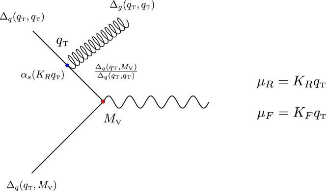
Figure 4.1: Drell-Yan production in association with one jet. $M_{\scriptscriptstyle\mathrm{V}}$ is the invariant mass of the vector boson, $q_{\scriptscriptstyle\mathrm{T}}$ is the transverse momentum of the jet (or the vector boson). We have attached Sudakov form factors, $\Delta_{s}$, according to the MiNLO procedure as outlined above. The strong coupling associated with the emitted gluon is evaluated in $K_{R}q_{\scriptscriptstyle\mathrm{T}}$. The renormalisation and factorisation scales are set to $\mu_{R}=K_{R}q_{\scriptscriptstyle\mathrm{T}}$ and $\mu_{F}=K_{F}q_{\scriptscriptstyle\mathrm{T}}$ respectively.

In order to further study the MiNLO modified $\bar{\mathcal{B}}$ function we turn to the production of a massive vector boson associated with one jet, Vj as shown in Figure 4.1. In this case we have $m=0$ and $n=1$. We cluster with the $k_{\scriptscriptstyle\mathrm{T}}$-algorithm setting the radius parameter $R=1$. Since there is only one branching in this process at Born-level, the lowest clustering scale, $Q_{0}$, is simply the transverse momentum of the emitted parton, which is equal to the transverse momentum of the vector boson, $q_{\scriptscriptstyle\mathrm{T}}$. The primary scale, $Q$, is taken to be the invariant mass of the vector boson, $M_{\scriptscriptstyle\mathrm{V}}$. Using the procedure described above, we find

$$\mathcal{F}(q_{\scriptscriptstyle\mathrm{T}};M_{\scriptscriptstyle\mathrm{V}})=\Delta_{q}(q_{\scriptscriptstyle\mathrm{T}},q_{\scriptscriptstyle\mathrm{T}})\Delta_{g}(q_{\scriptscriptstyle\mathrm{T}},q_{\scriptscriptstyle\mathrm{T}})\Delta_{q}(q_{\scriptscriptstyle\mathrm{T}},M_{\scriptscriptstyle\mathrm{V}})\frac{\Delta_{q}(q_{\scriptscriptstyle\mathrm{T}},M_{\scriptscriptstyle\mathrm{V}})}{\Delta_{q}(q_{\scriptscriptstyle\mathrm{T}},q_{\scriptscriptstyle\mathrm{T}})}=\Delta^{2}_{q}(q_{\scriptscriptstyle\mathrm{T}},M_{\scriptscriptstyle\mathrm{V}}),$$ (4.15)

and hence

$$\mathcal{F}^{(1)}(q_{\scriptscriptstyle\mathrm{T}};M_{\scriptscriptstyle\mathrm{V}})=2\Delta^{(1)}_{q}(q_{\scriptscriptstyle\mathrm{T}},M_{\scriptscriptstyle\mathrm{V}}).$$ (4.16)

The MiNLO modified $\bar{\mathcal{B}}$ function is then given by

$$\bar{\mathcal{B}}_{{\texttt{MiNLO}}{}} =\alpha_{s}(K_{R}q_{\scriptscriptstyle\mathrm{T}})\Delta^{2}_{q}(q_{\scriptscriptstyle\mathrm{T}},M_{\scriptscriptstyle\mathrm{V}})\bigg{[}B+$$

$$\alpha_{s}(K_{R}q_{\scriptscriptstyle\mathrm{T}})\left(V(\mu)+\int d\Phi_{r}R+B\left(\beta_{0}\ln\frac{K_{R}^{2}q_{\scriptscriptstyle\mathrm{T}}^{2}}{\mu^{2}}-2\Delta^{(1)}_{q}(q_{\scriptscriptstyle\mathrm{T}},M_{\scriptscriptstyle\mathrm{V}})\right)\right)\bigg{]},$$ (4.17)

where $\mu$ is some fixed scale which we will take to be the on-shell mass of the vector boson in our implementation. As already discussed above, this formula will lead to NLO accurate Vj production, but it is not entirely clear how accurate our expression is, when the hardest jet becomes unresolved. In the original MiNLO paper [158] this question was not addressed formally but very good behaviour of the predictions in the Sudakov peak regions were observed even for observables which should not obviously benefit from the MiNLO procedure. It was later shown that by modifying the MiNLO procedure slightly, the Vj generator would retain NLO accuracy even in the Sudakov peak region. Hence the Vj-MiNLO generator would effectively have merged an NLO V sample with an NLO Vj sample. We say that the Vj-MiNLO generator is both $\text{NLO}^{(0)}$ and $\text{NLO}^{(1)}$ accurate where $0,1$ refers to the number of resolved jets.

The modification which is needed to the MiNLO procedure is very simple as we will see shortly. However to show that the Vj-MiNLO generator is $\text{NLO}^{(0)}$ accurate is fairly involved and we shall not reproduce the proof of [159] here. We will however arrive at the same conclusion as the proof through naive power counting. We start by defining $L=\ln Q_{0}^{2}/Q^{2}$ and then rewrite Equation 4.7 as

$$\Delta_{f}(Q_{0},Q)=1+\alpha_{s}\left(-\frac{1}{2}A_{1}L^{2}+B_{1}L\right)+\mathcal{O}(\alpha_{s}^{2}).$$ (4.18)

As an expansion in $\alpha_{s}$ the $A_{1}$ and $B_{1}$ terms are equally important, but near the Sudakov peak $L$ becomes large, and the $A_{1}$ term starts dominating. We will take the Sudakov peak to mean $\alpha_{s}L^{2}\sim 1$. In this limit the above expansion is not a good one as higher order terms of the form $(\alpha_{s}L^{2})^{n}$ become as important as the leading order term. Of course the full Sudakov form factor correctly takes care of these higher order terms, but here we will use the expansion to quantify the precision of the calculation in the Sudakov peak region.

Observe first that

$$\alpha_{s}L^{2}\sim 1\quad\Rightarrow\quad L\sim\alpha_{s}^{-1/2},$$ (4.19)

which means that the term proportional to $B_{1}$ goes as $\alpha_{s}L\sim\alpha_{s}^{1/2}$. A necessary condition for the Vj-MiNLO generator to be $\text{NLO}^{(0)}$ accurate is that we are only neglecting terms of $\mathcal{O}(\alpha_{s}^{2})$. Further expanding the Sudakov form factor we get

$$\ln\Delta_{f}(Q_{0},Q)=$$

$$\qquad\alpha_{s}\left(-\frac{1}{2}[A_{1}+\alpha_{s}A_{2}+\alpha_{s}^{2}A_{3}]L^{2}+[B_{1}+\alpha_{s}B_{2}+\alpha_{s}^{2}B_{3}]L\right)+\dots$$ (4.20)

from which we easily read off that the $A_{2}$ term is $\mathcal{O}(\alpha_{s})$, the $B_{2}$ term is $\mathcal{O}(\alpha_{s}^{3/2})$, the $A_{3}$ term is $\mathcal{O}(\alpha_{s}^{2})$, and the $B_{3}$ term is $\mathcal{O}(\alpha_{s}^{5/2})$. Hence by including the $B_{2}$ term in the Sudakov form factor in addition to the $A_{1}$, $A_{2}$, and $B_{1}$ terms, we fulfil the condition that only terms of $\mathcal{O}(\alpha_{s}^{2})$ are neglected.

In addition to including the $B_{2}$ term in our Sudakov form factor, we also find it useful to specify how the Sudakov form factor behaves when the renormalisation scale is varied up and down around the central scale. This variation can be absorbed into a redefinition of the $A$ and $B$ coefficients given by [159]

$$\tilde{A}_{1} =A_{1}$$ (4.21)

$$\tilde{A}_{2} =A_{2}+2A_{1}\beta_{0}\ln K_{R}$$ (4.22)

$$\tilde{B}_{1} =B_{1}+2A_{1}\ln K_{R}$$ (4.23)

$$\tilde{B}_{2} =B_{2}+n\beta_{0}^{2}\ln K_{R}+2A_{2}\ln K_{R}+2A_{1}\beta_{0}\ln^{2}K_{R}.$$ (4.24)

4.3 NNLOPS Accurate Drell-Yan Production

During Run I of the LHC, at $7$ and then $8\;\mathrm{TeV}$ centre of mass energy, both the ATLAS and CMS collaboration collected almost $30\;\mathrm{fb}^{-1}$ of data. Because of their very large cross-sections and the very small systematic uncertainties, Drell-Yan production through $W$ and $Z$ exchange are standard candles at the LHC. Given the high-statistics reached, kinematic distributions can be studied over many orders of magnitude. With Run II at $13\;\mathrm{TeV}$ even more $W$ and $Z$ events have become available [179], and in particular it will be possible to study distributions over an even larger kinematic range. These distributions provide important input to constrain parton distribution functions. For example the rapidity distribution and the dilepton invariant mass of both neutral and charged Drell-Yan data have been used recently to constrain the photon content of the proton [84].

Higher-order corrections are indispensable for these studies, and Drell-Yan production is to date the theoretically best described process at the LHC. The cross-section is known through next-to-next-to-leading order (NNLO) in QCD including the decay of $W$ and $Z$ bosons to leptons [180, 181, 182]. Two public codes exist (DYNNLO [182] and FEWZ [183]) that implement QCD NNLO corrections to the hadronic $W$ and $Z$ production. Furthermore electroweak corrections have been the subject of intensive studies [184, 185, 186, 187, 188, 189]. Electroweak Sudakov effects become more important at large invariant mass [190, 191, 187, 192], a region that was already interesting at Run I and which is being explored even more during the current Run II of the LHC. Version 3 of FEWZ [193] implements also NLO EW corrections and the leading photon initiated processes. Recently, a framework for the calculation of the mixed QCD-electroweak ${\mathcal{O}}(\alpha_{s}\alpha)$ corrections to Drell-Yan processes in the resonance region has been developed [194, 195]. The impact of non-factorising (initial-final state) corrections is shown to be very small. Factorisable ${\mathcal{O}}(\alpha_{s}\alpha_{ew})$ corrections in the pole approximation have been computed. While QCD corrections are predominantly initial state corrections, and EW contributions are predominantly final-state corrections, because of kinematic effects there are sizeable differences between the result of Reference [194] and the naive product of NLO QCD and NLO EW corrections.

Having constructed a Drell-Yan generator which is $\text{NLO}^{(0)}$, $\text{NLO}^{(1)}$, and $\text{LO}^{(2)}$ accurate it is obvious to ask if it is possible to reweight the Vj-MiNLO events such that they exhibit $\text{NNLO}^{(0)}$ accuracy without spoiling the $\text{NLO}^{(1)}$ and $\text{LO}^{(2)}$ accuracy. We will here show that it is indeed possible. The argument was first presented in [159] and then refined in [113] for gluon fusion Higgs production. Here we discuss how the procedure works for Drell-Yan production.

Our implementation relies on the following inputs:

• Les Houches events for the $Z$+one jet or $W$+one jet process [146] (respectively Zj and Wj from now on), as implemented in POWHEG, upgraded with the improved MiNLO procedure described in Section 4.1 in such a way that NLO accuracy is guaranteed for inclusive distributions without any jet cut;

• NNLO accurate distributions, differential in the Born kinematics of the leptons, as obtained from DYNNLO [182];

• a local reweighting procedure, described in details in Section 4.3.1 below.

Compared with the standard NLOPS implementation of $W$ and $Z$ in POWHEG we find considerably reduced theoretical uncertainties for inclusive distributions. This is expected since our predictions have full NNLO accuracy. Furthermore the 1-jet region is described at NLO accuracy in our framework, even at small transverse momentum.

Throughout this work we pay particular attention to the issue of assigning a theory uncertainty to our predictions. We describe our procedure in Section 4.3.2.1. Unlike the standard POWHEG approach (without a separation between singular and finite real contributions), that is known to underestimate the theoretical uncertainty for the $W$, $Z$ or Higgs boson transverse momentum [196], we believe that our uncertainties are more reliable. Compared with pure NNLO predictions, we find in general a better description of observables sensitive to multiple emissions, such as the boson transverse momentum, $\phi^{*}$, and jet-resolution variables $d_{i}$ (which just vanish at NNLO starting from $i=2$). This is both because of the underlying MiNLO procedure, and because of the POWHEG framework.

4.3.1 NNLOPS Reweighting

We denote by $d\sigma^{{\scriptscriptstyle\mathrm{MINLO}}}/d\Phi$ the cross-section obtained from the Vj-MiNLO event generator, fully differential in the final state phase space, $\Phi$, at the level of the hardest emission events, i.e. before parton shower. Because of the properties of MiNLO, upon integration, this distribution reproduces the next-to-leading order accurate, $\mathcal{O}\left(\alpha_{s}\right)$, leptonic distributions inclusive in all QCD radiation. After integration over all QCD radiation only the leptonic system is left. This can be characterised by three independent variables, for instance one can choose the invariant mass of the lepton pair, $m_{\mathrm{ll}}$, the rapidity of the boson before decay $y_{V}$, and the angle of the negatively (or positively) charged lepton with respect to the beam, $\theta_{l}$. In the following we will use $\Phi_{B}$ to denote the ensemble of these three Born variables.

We denote schematically the fixed order NNLO cross-section differential over $\Phi_{B}$ by $d\sigma^{{\scriptscriptstyle\mathrm{NNLO}}}/d\Phi_{B}$ and the cross-section obtained from Vj-MiNLO by $d\sigma^{{\scriptscriptstyle\mathrm{MINLO}}}/d\Phi_{B}$. Since these distributions are identical up to terms of $\mathcal{O}\left(\alpha_{s}\right)$, their ratio is equal to one up to $\mathcal{O}\left(\alpha_{{\scriptscriptstyle\mathrm{S}}}^{2}\right)$ terms:

$$\mathcal{W}(\Phi_{B})=\frac{\frac{d\sigma^{\scriptscriptstyle\mathrm{NNLO}}}{d\Phi_{B}}}{\frac{d\sigma^{\scriptscriptstyle\mathrm{MINLO}}}{d\Phi_{B}}}=\frac{c_{0}+c_{1}\alpha_{{\scriptscriptstyle\mathrm{S}}}+c_{2}\alpha_{{\scriptscriptstyle\mathrm{S}}}^{2}\phantom{+\ldots}}{c_{0}+c_{1}\alpha_{{\scriptscriptstyle\mathrm{S}}}+c_{2}^{\prime}\alpha_{{\scriptscriptstyle\mathrm{S}}}^{2}+\ldots}=1+\frac{c_{2}-c_{2}^{\prime}}{c_{0}}\,\alpha_{{\scriptscriptstyle\mathrm{S}}}^{2}+\ldots\,,$$ (4.25)

where the $c_{i}$ are $\mathcal{O}\left(1\right)$ coefficients. Since the Vj-MiNLO generator reproduces the inclusive fixed-order result up to and including NLO terms, the NLO accuracy of the cross-section in the presence of one jet (that starts at order $\alpha_{s}$) is maintained if the cross-section is reweighed by the factor in Equation 4.25. This follows from the simple fact that the reweighting factor combined with this cross-section yields spurious terms of $\mathcal{O}(\alpha_{s}^{3})$ and higher.

It is also obvious that by reweighting Vj-MiNLO distributions with this ratio, any of the three $\Phi_{B}$ distributions acquire NNLO accuracy, and in fact coincide with the NNLO distributions. We will now argue that the Vj-MiNLO generator reweighed with the procedure of Equation 4.25 maintains the original NNLO accuracy of the fixed-order program, used to obtain the $d\sigma^{\scriptscriptstyle\mathrm{NNLO}}/d\Phi_{B}$ distribution, for all observables. The proof trivially extends the proof given in Reference [113] by replacing the Higgs rapidity with the chosen set of three variables $\Phi_{B}$ associated with the Born phase space.

The claim is based on the following theorem:

A parton level V boson production generator that is accurate at ${\mathcal{O}}(\alpha_{{\scriptscriptstyle\mathrm{S}}}^{2})$ for all IR safe observables that vanish with the transverse momenta of all light partons, and that also reaches ${\mathcal{O}}(\alpha_{{\scriptscriptstyle\mathrm{S}}}^{2})$ accuracy for the three Born variables $\Phi_{B}$ achieves the same level of precision for all IR safe observables, i.e. it is fully NNLO accurate.

To this end, we consider a generic observable $F$, including cuts, that is an infrared safe function of the final state kinematics. $F$ could for instance be a bin of some distribution. Its value will be given by

$$\langle F\rangle=\int d\Phi\,\frac{d\sigma}{d\Phi}\,F(\Phi)$$ (4.26)

with a sum over final state multiplicities being implicit in the phase space integral. Infrared safety ensures that $F$ has a smooth limit when the transverse momenta of the light partons vanish.

Since the Born kinematics are fully specified by the Born variables $\Phi_{B}$, such a limit may only depend upon the value of Born kinematic variables $\Phi_{B}$. We generically denote such a limit by $F_{\Phi_{B}}$. The value of $\langle F\rangle$ can be considered as the sum of two terms: $\left\langle F-F_{\Phi_{B}}\right\rangle+\left\langle F_{\phi_{B}}\right\rangle$. Since $F-F_{\Phi_{B}}$ tends to zero with the transverse momenta of all the light partons, by hypothesis its value is given with ${\mathcal{O}}(\alpha_{{\scriptscriptstyle\mathrm{S}}}^{2})$ accuracy by the parton level generator. We may also write

$$\left\langle F_{\Phi_{B}}\right\rangle=\int d\Phi_{B}^{\prime}\,\frac{d\sigma}{d\Phi_{B}^{\prime}}\,F_{\Phi_{B}}\left(\Phi_{B}^{\prime}\right)\,,$$ (4.27)

which is exact at the ${\mathcal{O}}(\alpha_{{\scriptscriptstyle\mathrm{S}}}^{2})$ level by hypothesis. Thus, $\langle F\rangle=\left\langle F-F_{\Phi_{B}}\right\rangle+\left\langle F_{\Phi_{B}}\right\rangle$ is accurate at the ${\mathcal{O}}(\alpha_{{\scriptscriptstyle\mathrm{S}}}^{2})$ level.

The Vj-MiNLO parton level generator (in fact even just Vj) fulfils the first condition of the theorem, since it predicts any IR safe observable that vanishes, when the transverse momenta of the light partons vanish, with $\mathcal{O}(\alpha_{s}^{2})$ accuracy. The second hypothesis of the theorem, regarding NNLO accuracy of the Born variables, is simply realised by augmenting the Vj-MiNLO generator by the reweighting procedure described above. We note that MiNLO is crucial to preserve the first property after rescaling. The proof of $\mathcal{O}(\alpha_{s}^{2})$ accuracy for these observables thus corresponds to the general proof of NLO accuracy of the POWHEG procedure, given in References [73, 86].

Note that for observables of the type $\left\langle F-F_{\Phi_{B}}\right\rangle$, adding the full shower development does not alter the $\mathcal{O}(\alpha_{s}^{2})$ accuracy of the algorithm, for the same reasons as in the case of the regular POWHEG method. The only remaining worry one can have, concerns the possibility that the inclusive Born variable distributions are modified by the parton shower evolution at the level of $\mathcal{O}(\alpha_{s}^{2})$ terms. However, our algorithm already controls the two hardest emissions with the required $\alpha_{s}^{2}$ accuracy. A further emission from the shower is thus bound to lead to corrections of higher order in $\alpha_{s}$. This concludes our proof.

4.3.1.1 Variant Schemes

As discussed in detail in Reference [113] the reweighting in Equation 4.25 treats low and high transverse momentum distributions equally, i.e. it distributes the virtual correction over the full transverse momentum range considered. On the other hand, if one considers the transverse momentum distribution of the vector boson $V$ or of the leading jet, in the high transverse-momentum region Vj-MiNLO and the NNLO calculation have formally the same (NLO) accuracy. Hence, while it is not wrong to do so, there is no need to “correct” the Vj-MiNLO result in that region. It is therefore natural to introduce a function that determines how the two-loop virtual correction is distributed over the whole transverse momentum region,

$$h(p_{\scriptscriptstyle\mathrm{T}})=\frac{(\beta\,M_{{\scriptscriptstyle\mathrm{V}}})^{\gamma}}{(\beta\,M_{{\scriptscriptstyle\mathrm{V}}})^{\gamma}+p_{\scriptscriptstyle\mathrm{T}}^{\gamma}},$$ (4.28)

where $\beta$ and $\gamma$ are constant parameters, and $M_{{\scriptscriptstyle\mathrm{V}}}$ is the mass of the vector boson. This function has the property that when $p_{\scriptscriptstyle\mathrm{T}}$ goes to zero it tends to one, while when $p_{\scriptscriptstyle\mathrm{T}}$ becomes very large, it vanishes.

The function $h(p_{\scriptscriptstyle\mathrm{T}})$ can therefore be used to split the cross-section according to

$$d\sigma_{\phantom{0}} = d\sigma_{A}+d\sigma_{B}\,,$$ (4.29)

$$d\sigma_{A} = d\sigma\,h\left(p_{\scriptscriptstyle\mathrm{T}}\right)\,,$$ (4.30)

$$d\sigma_{B} = d\sigma\,\left(1-h\left(p_{\scriptscriptstyle\mathrm{T}}\right)\right)\,.$$ (4.31)

We then reweight the Vj-MiNLO prediction using the following factor

$$\mathcal{W}\left(\Phi_{B},\,p_{{\scriptscriptstyle\mathrm{T}}}\right) = h\left(p_{\scriptscriptstyle\mathrm{T}}\right)\,\frac{\smallint d\sigma^{{\scriptscriptstyle\mathrm{NNLO\phantom{i}}}}\,\delta\left(\Phi_{B}-\Phi_{B}\left(\Phi\right)\right)-\smallint d\sigma_{B}^{{\scriptscriptstyle\mathrm{MINLO}}}\,\delta\left(\Phi_{B}-\Phi_{B}\left(\Phi\right)\right)}{\smallint d\sigma_{A}^{{\scriptscriptstyle\mathrm{MINLO}}}\,\delta\left(\Phi_{B}-\Phi_{B}\left(\Phi\right)\right)}$$ (4.32)

$$+ \left(1-h\left(p_{\scriptscriptstyle\mathrm{T}}\right)\right)\,,$$

which preserves the exact value of the NNLO cross-section

$$\left(\frac{d\sigma}{d\Phi_{B}}\right)^{{\scriptscriptstyle\mathrm{NNLOPS}}} = \left(\frac{d\sigma}{d\Phi_{B}}\right)^{{\scriptscriptstyle\mathrm{NNLO}}}\,.$$ (4.33)

The proof of NNLO accuracy for this rescaling scheme is completely analogous to the proof given above, so we omit it here.

4.3.2 Phenomenological Analysis

In this section, in order to validate our results, we make a number of comparisons with fixed-order calculations and dedicated resummations. In particular, we find good agreement between our NNLOPS calculations and DYqT [197] for the $Z$ transverse momentum distribution. We also compare our results for the $\phi^{*}$ distribution to the NLO+NNLL resummation of Reference [198], and the jet-veto efficiency with the NNLL+NNLO results of Reference [199].

An implementation of Drell-Yan lepton pair production at NNLO accuracy including parton shower effects using the UN²LOPS algorithm in the event generator Sherpa was recently presented in Reference [171]. An important difference of this implementation with respect to our approach, is that in Reference [171] the pure NNLO correction sits in the bin where the $Z$ boson has zero transverse momentum. These events do not undergo any parton showering, populating only the zero-$p_{\scriptscriptstyle\mathrm{T}}$ bin. Thus, in the approach of Reference [171], the $Z$ boson transverse momentum is insensitive to the NNLO correction.

A general approach to matching NNLO computations with parton showers was also proposed in Reference [170]. The MiNLO procedure that we use in this work was discussed by the authors of Reference [170] in the context of the general formulation of their method. Given that an implementation of Reference [170] now exists for Drell-Yan production [200], it will be interesting to see how the three different matching schemes compare.

Before showing our validation results, we define our procedure for estimating theoretical uncertainties.

4.3.2.1 Estimating Uncertainties

As is standard, the uncertainties in the Vj-MiNLO generator are obtained by varying the renormalisation scales appearing in the MiNLO procedure by $K_{\scriptscriptstyle\mathrm{R}}$ and the factorisation scale by $K_{\scriptscriptstyle\mathrm{F}}$, by a factor 2 up and down keeping $1/2\leq K_{\scriptscriptstyle\mathrm{R}}/K_{\scriptscriptstyle\mathrm{F}}\leq 2$. This leads to 7 different scale choices given by

$$(K_{{\scriptscriptstyle\mathrm{R}}},K_{{\scriptscriptstyle\mathrm{F}}})=(0.5,0.5),(1,0.5),(0.5,1),(1,1),(2,1),(1,2),(2,2)\,.$$ (4.34)

We will consider the variation in our results induced by the above procedure. The seven scale variation combinations have been obtained by using the reweighting feature of the POWHEG-BOX.

For the pure NNLO results, the uncertainty band is the envelope of the 7-scale variation obtained by varying the renormalisation and factorisation scale by a factor 2 around the central value $M_{V}$ keeping $1/2\leq K_{\scriptscriptstyle\mathrm{R}}/K_{\scriptscriptstyle\mathrm{F}}\leq 2$.

For the NNLOPS results, we have first generated a single of Zj-MiNLO event file with all the weights needed to compute the integrals $d\sigma_{A/B}^{\scriptscriptstyle\mathrm{MINLO}}/d\Phi_{B}$, in Equation 4.32, for all 7 scale choices. The differential cross-section $d\sigma^{\scriptscriptstyle\mathrm{NNLO}}/d\Phi$ was tabulated for each of the three scale variation points corresponding to $K_{\scriptscriptstyle\mathrm{R}}^{\prime}=K_{\scriptscriptstyle\mathrm{F}}^{\prime}$. The analysis is then performed by processing the MiNLO event for given values of $(K_{\scriptscriptstyle\mathrm{R}},K_{\scriptscriptstyle\mathrm{F}})$, and multiplying its weight with the factor

$$h\left(p_{\scriptscriptstyle\mathrm{T}}\right)\times\,\frac{\smallint d\sigma_{(K_{\scriptscriptstyle\mathrm{R}}^{\prime},K_{\scriptscriptstyle\mathrm{F}}^{\prime})}^{{\scriptscriptstyle\mathrm{NNLO\phantom{i}}}}\,\delta\left(\Phi_{B}-\Phi_{B}(\Phi)\right)-\smallint d\sigma_{B,(K_{\scriptscriptstyle\mathrm{R}},K_{\scriptscriptstyle\mathrm{F}})}^{{\scriptscriptstyle\mathrm{MINLO}}}\,\delta\left(\Phi_{B}-\Phi_{B}(\Phi)\right)}{\smallint d\sigma_{A,(K_{\scriptscriptstyle\mathrm{R}},K_{\scriptscriptstyle\mathrm{F}})}^{{\scriptscriptstyle\mathrm{MINLO}}}\,\delta\left(\Phi_{B}-\Phi_{B}(\Phi)\right)}+\left(1-h\left(p_{\scriptscriptstyle\mathrm{T}}\right)\right)\,.$$ (4.35)

The central value is obtained by setting $(K_{\scriptscriptstyle\mathrm{R}},K_{\scriptscriptstyle\mathrm{F}})$ and $(K_{\scriptscriptstyle\mathrm{R}}^{\prime},K_{\scriptscriptstyle\mathrm{F}}^{\prime})$ equal to one, while to obtain the uncertainty band we apply this formula for all the seven $(K_{{\scriptscriptstyle\mathrm{R}}},K_{{\scriptscriptstyle\mathrm{F}}})$ and three $(K_{{\scriptscriptstyle\mathrm{R}}}^{\prime},K_{{\scriptscriptstyle\mathrm{F}}}^{\prime})$ choices. This yields 21 variations at NNLOPS level.

The reasoning behind varying scales in the NNLO and Zj-MiNLO results independently is that we regard uncertainties in the overall normalisation of distributions, as being independent of the respective uncertainties in the shapes. This is consistent with the recently introduced efficiency method [201], used for estimating errors on cross-sections in the presence of cuts.

4.3.2.2 Practical Implementation

There is some degree of freedom in the way the reweighting procedure described above is carried out in practice. In particular, one is free to choose the three Born variables with respect to which one performs the reweighting, as well as the form of the damping factor $h$ in Equation 4.28. Our choice of the Born variables is driven by the fact that one wants to populate all bins in the three-dimensional histograms sufficiently well. To produce the results presented in the following we used the rapidity of the $Z$ boson, $y_{Z}$, a variable directly related to the dilepton invariant mass, $a_{\mathrm{mll}}=\mathrm{\arctan}((m_{\mathrm{ll}}^{2}-M_{\scriptscriptstyle\mathrm{Z}}^{2})/(M_{\scriptscriptstyle\mathrm{Z}}\Gamma_{Z}))$ and $\theta^{*}_{l}$, where the latter is the angle between the beam and a charged lepton in the frame where the boson has no longitudinal momentum.

In the following we will use the values of $\beta=1$ and $\gamma=2$ in Equation 4.28. The choice for $\beta$ is motivated by the fact that typical resummation scale for Drell-Yan production is set to the boson mass. The second choice is partly driven by the fact that in the case of Higgs production, with this choice the NNLOPS Monte Carlo agrees well with the Higgs transverse momentum and leading jet NNLL+NNLO resumed results. We stress however that while $\beta$ and $\gamma$ are arbitrary, the dependence on $\beta$ and $\gamma$ is formally ${\mathcal{O}}(\alpha_{s}^{3})$ (or exactly zero in the case of inclusive quantities). $p_{\scriptscriptstyle\mathrm{T}}$ in Equation 4.28 denotes the transverse momentum that is used to decide how to distribute the virtual corrections. One could for instance choose the $V$ transverse momentum, the leading jet transverse momentum, or the total transverse momentum of the event. In the following, we will adopt the choice of Reference [113], namely to use the leading jet transverse momentum when clustering events according to the inclusive $k_{\scriptscriptstyle\mathrm{T}}$-algorithm with $R=0.7$ [202]. This choice ensures that $h$ goes to one when no radiation is present, since in that case the leading jet transverse momentum vanishes. On the contrary, the $V$ transverse momentum can vanish also in the presence of radiation.

Finally we note that for the reweighting we used 25 bins per variable, meaning that our 3-dimensional distributions involve a total of $15625$ equal bins. Results presented in the following are based on generating 20 million events. Even if we perform high-statistics runs, there might be bins that are not well-populated. This can give rise to a rescaling factor that is unphysically large just because too few events ended up in one bin, and this in turn can give rise to spikes in kinematical distributions. To avoid these occurrences, instead of using the local reweighting factor, we use the global $K_{\mathrm{NNLO}}/K_{\mathrm{NLO}}$ factor to perform the reweighting whenever the local reweighting factor (which is formally $1+{\mathcal{O}}(\alpha_{s})^{2}$) exceeds 5. This happens rarely, in about 0.3% of the points. We checked that this procedure has no visible systematic effect on distributions, other than that of removing unphysical spikes. Other workarounds could of course also be adopted.

Before showing validation plots, we list here the settings used for the results obtained in this Chapter. We used the code DYNNLO [182] to obtain NNLO predictions. Throughout this work we consider the MSTW2008NNLO parton distribution functions [148] and set $M_{\scriptscriptstyle\mathrm{Z}}=91.1876\;\mathrm{GeV}$, $\Gamma_{Z}=2.49595\;\mathrm{GeV}$, $M_{\scriptscriptstyle\mathrm{W}}=80.398$ GeV and $\Gamma_{W}=2.008872\;\mathrm{GeV}$. We choose to use $\alpha_{\mathrm{em}}=1/128.94$ and $\sin^{2}\theta_{W}=0.22264585$. Jets have been constructed using FastJet [150, 76]. To compute the $h(p_{\scriptscriptstyle\mathrm{T}})$ factor we use the $k_{\scriptscriptstyle\mathrm{T}}$- algorithm [202, 203] with $R=0.7$. To shower partonic events, we have used both PYTHIA8 [204] (version 8.185) with the “Monash 2013” [205] tune and PYTHIA6 (version 6.4.28) with the MSTW2008LO variation of the “Perugia” tune (“Perugia P12-M8LO”, tune 378). We have generated $Z$ and $W$ events with decays into electrons and positrons, and always switched off QED radiation off leptons and quarks in the showering stage. Moreover, in the following, in order to define the leptons from the boson decays we will always use the Monte Carlo truth, i.e. we disregard complications due to the fact that there might be other leptons in the event.

To obtain the results shown in the following, we have switched on the “doublefsr” option introduced in Reference [206] and used a standard driver for PYTHIA6 and the PYTHIA8 driver suggested by the PYTHIA authors for showering events generated with POWHEG. Although we have also explored the effect of using the alternative prescription first introduced in Section 4 of Reference [206] to compute the scale used by the parton shower to veto hard emissions (which is also available as an option in the PYTHIA8 driver), the plots shown throughout the chapter have been obtained keeping the veto scale equal to the default POWHEG prescription, both for PYTHIA6 and PYTHIA8.

4.3.2.3 Validation Plots

In this section we consider the case of inclusive $Z\to e^{+}e^{-}$ production at 14 TeV, with no cuts on the final state other than requiring the dilepton invariant mass to be in the range $66\;\mathrm{GeV}\leq m_{\mathrm{ll}}\leq 116\;\mathrm{GeV}$. In order to validate our results, we will show comparisons to NNLO predictions and to MiNLO-improved Zj-POWHEG results (henceforth denoted as Zj-MiNLO). Since we compare with DYNNLO, for the Zj-MiNLO and NNLOPS results it is useful to consider here pure parton level results before hadronisation (with underlying event and multiparton interaction switched off). Unless otherwise stated, for DYNNLO we have set $\mu_{\mathrm{F}}=\mu_{\mathrm{R}}=M_{\scriptscriptstyle\mathrm{Z}}$, and the associated uncertainty bands are obtained from a 7-points scale variation envelope. Also unless stated otherwise, we will shower events with PYTHIA8.

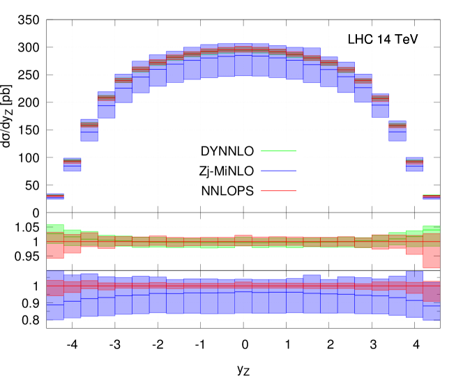
Figure 4.2: Comparison of the NNLOPS (red), Zj-MiNLO (blue) and DYNNLO (green) results for the $Z$ boson fully inclusive rapidity distribution at the LHC running at 14 TeV. The DYNNLO central scale is $\mu_{\mathrm{F}}=\mu_{\mathrm{R}}=M_{\scriptscriptstyle\mathrm{Z}}$, and its error band is the 7-point scale variation envelope. For NNLOPS and Zj-MiNLO the procedure to define the scale uncertainty is described in detail in Section 4.3.2.1. The two lower panels show the ratio of DYNNLO and Zj-MiNLO predictions with respect to NNLOPS obtained with its central scale choice.

In Figure 4.2 we show the $Z$ boson rapidity distribution $y_{Z}$ as predicted at NNLO (green), with Zj-MiNLO (blue), and at NNLOPS (red). As expected NNLOPS agrees very well with DYNNLO over the whole rapidity range, both for the central value and the uncertainty band, defined as detailed in Section 4.3.2.1. We also note that as expected, the uncertainty band of the NNLOPS result is considerably reduced compared with the one of Zj-MiNLO, which is NLO accurate. In the central region the uncertainty decreases from about $(+5:-15)\%$ to about $(+2:-2)\%$. We finally note that because of the positive NNLO corrections, the central value of NNLOPS lies about 5 % above the one of Zj-MiNLO, while no considerably difference in shape is observed in the central rapidity region. Moderate but slightly more pronounced shape differences can be seen at large rapidity.

We proceed by examining the other two distributions that have been used in the reweighting procedure, namely $a_{\mathrm{m_{\mathrm{ll}}}}$ and $\theta^{*}_{l}$. Instead of showing $a_{\mathrm{m_{\mathrm{ll}}}}$ we plot in Figure 4.3 the invariant mass of the dilepton system $m_{\mathrm{ll}}$ which is directly related to $a_{\mathrm{m_{\mathrm{ll}}}}$. We notice that the same features observed above hold: NNLOPS agrees well with DYNNLO, it tends to be about 5$-$10% higher than Zj-MiNLO and the uncertainty band is reduced by about a factor 4. No sizeable difference in shape is observed in these two distributions, when comparing Zj-MiNLO and NNLOPS.

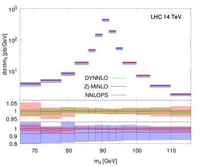
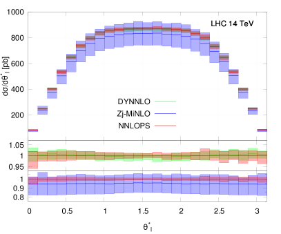
Figure 4.3: As for Figure 4.2 but for $m_{\mathrm{ll}}$ (left) and $\theta_{l}^{*}$ (right).

We now show in Figure 4.4 the $Z$ boson transverse momentum in two different ranges. At finite values of $p_{\scriptscriptstyle\mathrm{T,Z}}$ this quantity is described at NLO accuracy only by all three codes, DYNNLO, NNLOPS and Zj-MiNLO. In fact, at higher value of $p_{\scriptscriptstyle\mathrm{T,Z}}$ the bands of NNLOPS and Zj-MiNLO overlap and are very similar in size.

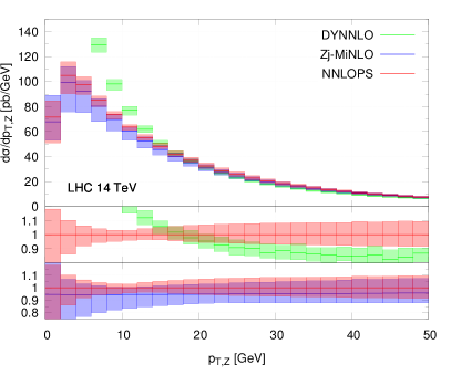
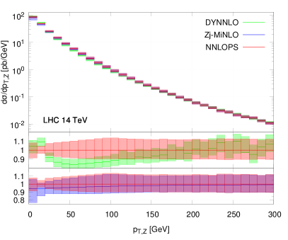
Figure 4.4: As for Figure 4.2 but for the $Z$-boson transverse momentum for two different ranges in $p_{\scriptscriptstyle\mathrm{T,Z}}$.

At small transverse momenta, while DYNNLO diverges, NNLOPS remains finite because of the Sudakov damping. The difference in shape observed between DYNNLO and NNLOPS at finite $p_{\scriptscriptstyle\mathrm{T,Z}}$ has to do with the fact that in that region the fixed-order calculation has to compensate for the divergent behaviour at small $p_{\scriptscriptstyle\mathrm{T,Z}}$. We also note that the uncertainty band in DYNNLO is far too small when approaching the divergence at $p_{\scriptscriptstyle\mathrm{T,Z}}=0$. The uncertainty band of NNLOPS instead tends to increase at very low transverse momenta, reflecting the fact that one is approaching a non-perturbative region. One can however also note that the uncertainty tends to shrink at about $p_{\scriptscriptstyle\mathrm{T,Z}}=10\;\mathrm{GeV}$. We have checked that this is not an artefact due to having used a 21-point scale variation as opposed to a 49-point one. We attribute this feature to the fact that the uncertainty band of the fixed-order result shrinks in this region. This is true both for the 3-point and the 7-point scale variation in the fixed order, although in the latter case this effect is slightly less pronounced. We also observe that our Zj-MiNLO result that uses the MiNLO scale prescription does not show this feature. When we upgrade Zj-MiNLO to NNLO accuracy, we necessarily inherit this feature from the NNLO results we are using as input. It is also worth mentioning that this feature has been already observed in several studies where an analytic resummation matched with fixed-order results was performed for this observable [197, 207, 208].

We end our discussion on neutral Drell-Yan production by looking briefly into the effects of including non-perturbative contributions in the NNLOPS simulation, by turning on hadronisation, underlying event and multiparton interaction (MPI). In particular, given the small perturbative uncertainties found with $p_{\scriptscriptstyle\mathrm{T,Z}}$, it is interesting to see how much non-perturbative corrections affect the $5-15\;\mathrm{GeV}$ region.

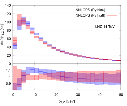
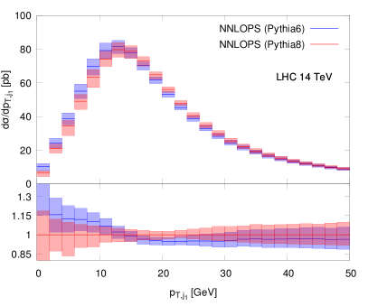
Figure 4.5: NNLOPS predictions for the transverse momentum of the reconstructed $Z$ boson (left) and leading jet (right) obtained using PYTHIA6 (blue) and PYTHIA8 (red). Non-perturbative effects have been included here, by using the tunes mentioned in Section 4.3.2.2.

In Figure 4.5 we show $p_{\scriptscriptstyle\mathrm{T,Z}}$ (left) and the leading-jet transverse momentum, defined according to the anti-$k_{\scriptscriptstyle\mathrm{T}}$ [75] algorithm with $R=0.7$ (right), after all non-perturbative stages are included, with PYTHIA6 (blue) and PYTHIA8 (red). We observe sizeable differences between the two results, in particular for the $Z$ boson transverse momentum at $p_{\scriptscriptstyle\mathrm{T,Z}}<15\;\mathrm{GeV}$. This is not surprising since this is a region dominated by soft effects, hence the details of the modelling of non-perturbative effects are expected to matter. For the jet-transverse momentum the difference between the two shower models is slightly smaller. This can probably be attributed to the fact that the Sudakov peak is at larger values of the transverse momentum, compared with the $Z$ boson transverse momentum.

Finally, for illustrative purposes, we conclude this section by showing in Figure 4.6 predictions for the transverse momentum (left) and pseudorapidity (right) of the charged electron or positron in $W$ production at 7 TeV (combining the $W^{+}$ and $W^{-}$ samples).

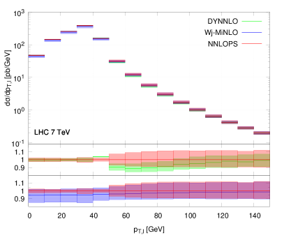
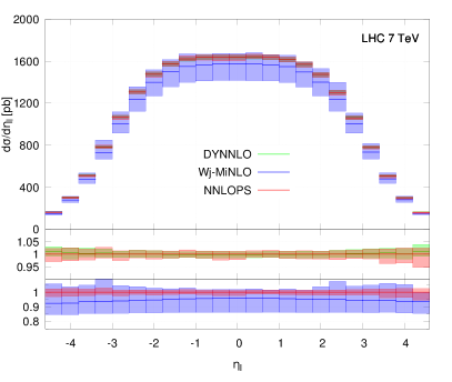
Figure 4.6: Comparison of the NNLOPS (red), Zj-MiNLO (blue) and DYNNLO (green) results for the transverse momentum (left) and rapidity distributions of the charged lepton (right) in $W$ production at the LHC running at 7 TeV. The DYNNLO central scale is $\mu_{\mathrm{F}}=\mu_{\mathrm{R}}=M_{\scriptscriptstyle\mathrm{W}}$, and its error band is the 3-point scale variation envelope. For NNLOPS and Zj-MiNLO the procedure to define the scale uncertainty is described in detail in Section 4.3.2.1. The lower panels show the ratio with respect to the NNLOPS prediction obtained with its central scale choice.

It is interesting to look at these leptonic observables since they don’t coincide with the quantities we are using to perform the NNLO reweighting. Nevertheless, we should recover NNLO accuracy in the regions where the lepton kinematics probes the fully-inclusive phase space: this is precisely what we have found, as illustrated in Figure 4.6. Here we include no cuts on the final state other than requiring the transverse $W$ mass $m_{\scriptscriptstyle\mathrm{T,W}}=\sqrt{2(p_{{\scriptscriptstyle\mathrm{T,l}}}\,p_{{\scriptscriptstyle\mathrm{T}},miss}-\vec{p}_{{\scriptscriptstyle\mathrm{T,l}}}\,\cdot\vec{p}_{{\scriptscriptstyle\mathrm{T}},miss})}$ to be larger than $40\;\mathrm{GeV}$. All parameters and settings are the same as those used for the $Z$ production case and DYNNLO results have been obtained choosing $\mu_{\mathrm{R}}=\mu_{\mathrm{F}}=M_{\scriptscriptstyle\mathrm{W}}$ as central scale and performing a 3-point scale variation.

As expected, in the left panel of Figure 4.6 we observe a much narrower uncertainty on the charged lepton transverse momentum for values of $p_{\mathrm{T,l}}$ smaller than $M_{\scriptscriptstyle\mathrm{W}}/2$, and a very good agreement with DYNNLO in this region, both in the absolute value of the cross-section as well as in the size of the theoretical uncertainty band. When $p_{\mathrm{T,l}}$ is larger than $M_{\scriptscriptstyle\mathrm{W}}/2$ all distributions have NLO accuracy only, since in this region the lepton kinematics requires non-vanishing values for $p_{\scriptscriptstyle\mathrm{T,W}}$. We observe that in fact all uncertainty bands are larger in this region. Our NNLOPS result reproduces the Zj-MiNLO one well, while there is some difference between DYNNLO and Zj-MiNLO predictions. This is expected since the scales used in the two calculations are effectively different: DYNNLO always uses the mass of the $W$ boson, whereas in MiNLO the transverse momentum of the $W$ boson is used. Therefore when the lepton is just slightly harder than $M_{\scriptscriptstyle\mathrm{W}}/2$ we are probing phase-space regions where the bulk of the cross-section typically has $0\lesssim p_{\scriptscriptstyle\mathrm{T,W}}\lesssim M_{\scriptscriptstyle\mathrm{W}}$, and hence DYNNLO yields smaller cross-sections.

It is also worth mentioning that both the NNLOPS and Zj-MiNLO plots exhibit a smooth behaviour in proximity of the Jacobian peak $p_{\mathrm{T,l}}\simeq M_{\scriptscriptstyle\mathrm{W}}/2$, also when thinner bins (not shown) are used. This smooth behaviour is due both to parton-shower effects and to the MiNLO Sudakov form factor. On the contrary, the NNLO prediction displays the typical numerical instability of fixed-order predictions due to the numerical cancellation between real and virtual corrections close to the kinematical boundary. Furthermore, the NNLO prediction has spuriously small uncertainties in this region.

Finally, in the right panel of Figure 4.6 we plot the rapidity distribution of the charged lepton. Since in each bin of this distribution we are fully inclusive with respect to QCD radiation, we observe the expected good agreement with the NNLO prediction over the whole range, as well as a quite narrow uncertainty band.

4.3.2.4 Comparison to Analytic Resummations

The MiNLO method at the core of the results presented in this chapter works by including NLL and (some) NNLL terms in the Sudakov form factors used to improve the validity and accuracy of the underlying NLO computation. Although the formal logarithmic accuracy achieved by MiNLO-improved POWHEG simulations has not been addressed, it is interesting to compare NNLOPS predictions against results obtained with higher-order analytic resummation, for observables where the latter are available. In this subsection we will show results for $Z$ production at 7 TeV and focus on three quantities for which NNLL resummation has been performed.

The classical observable to consider in Drell-Yan production to study the effects of soft-collinear radiation is the transverse momentum of the dilepton-pair system. This observable has been extensively studied in the past and is now known to NNLO+NNLL level [197, 207].

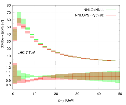
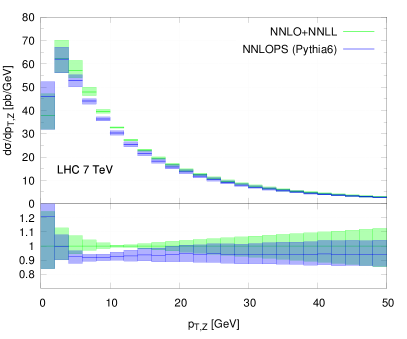
Figure 4.7: Comparison of NNLOPS prediction and NNLO+NNLL resummation for $p_{\scriptscriptstyle\mathrm{T,Z}}$ at the 7 TeV LHC. The NNLOPS prediction is shown at parton level with parton showering performed with PYTHIA8 (left, red) and PYTHIA6 (right, blue). The resummed result is shown in green in both panels. The lower panels show the ratio to the NNLO+NNLL resummation.

In Figure 4.7 we show a comparison between the NNLO+NNLL resummation obtained using DYqT and our NNLOPS result obtained with PYTHIA8 (left) and PYTHIA6 (right), switching off all non-perturbative effects (i.e. hadronisation and MPI are switched off, primordial-$k_{\scriptscriptstyle\mathrm{T}}$ is set to zero). As usual, the uncertainty band for our results has been obtained as the envelope of a 21-points scale variation. DYqT uses as resummation scale $m_{\textrm{ll}}$, and the associated band has been obtained varying $\mu_{\mathrm{R}}$ and $\mu_{\mathrm{F}}$ among the usual 7 combinations. On top of this, for the central value of $\mu_{\mathrm{R}}=\mu_{\mathrm{F}}$ we varied the resummation scale by a factor 2 up and down. This gives 9 combinations, the envelope of which is used here to define the DYqT uncertainty. The ratio plot shows a pattern quite similar to what was observed in Figures 4 and 5 of Reference [113], namely differences of up to $\mathcal{O}(10-12\%)$ between analytic resummation and NNLOPS, with a slightly more marked difference in the very first bin. In the region $p_{\scriptscriptstyle\mathrm{T,Z}}\sim 5-15\;\mathrm{GeV}$, the uncertainty bands do not overlap, mainly because of the very narrow uncertainty bands in both predictions, in particular in the NNLO+NNLL result. In the case of Higgs production, instead, uncertainty bands are wider, hence the predictions are more compatible. Changing the $\beta$ parameter might improve this agreement, although we recall that the NNLOPS prediction does not have NNLL accuracy in this region. By comparing the two NNLOPS results shown in the two panels of Figure 4.7, we also observe that the spectra obtained with PYTHIA8 are typically $\sim 5$ % harder than those with PYTHIA6, a feature that was already noticeable in Figure 4.5, and which will be present also in other distributions where NNLOPS results are “only” NLO accurate. Few percent differences between different NLO+PS results in these kinematic regions can be due to subleading effects, such as differences in details of the two parton-shower algorithms, as well as the use of different tunes.

Another interesting observable to consider is the $\phi^{*}$ distribution which is a measure of angular correlations in Drell-Yan lepton pairs [209]. This observable is defined as [208]

$$\phi^{*}=\tan\left(\frac{\pi-\Delta\phi}{2}\right)\sin\theta^{*}\,,$$ (4.36)

where $\Delta\phi$ is the azimuthal angle between the two leptons and $\theta^{*}$ is the scattering angle of the electron with respect to the beam, as computed in the boosted frame where the $Z$ boson is at rest. We note that ATLAS uses a slightly different definition of the angle $\theta^{*}$, and defines it as

$$\cos\theta^{*}=\mathrm{tanh}\left(\frac{y_{l^{-}}-y_{l^{+}}}{2}\right)\,.$$ (4.37)

Since we will compare with ATLAS data in Section 4.3.3.2, we will use the latter definition throughout this work.

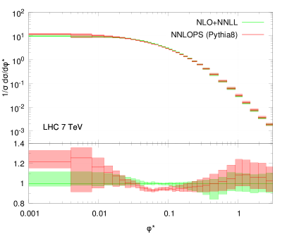
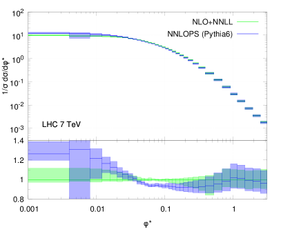
Figure 4.8: Comparison of NNLOPS prediction and NLO+NNLL resummation for $\phi^{*}$ in $Z\to e^{+}e^{-}$ production at 7 TeV LHC. The NNLOPS prediction is shown at parton level with parton showering performed with PYTHIA8 (left, red) and PYTHIA6 (right, blue). The resummed result is shown in green in both panels.

In Figure 4.8 we compare our NNLOPS simulation with the NLO+NNLL resummation of Reference [208]. From the definition of $\phi^{*}$, it is clear that large values of $\phi^{*}$ correspond to events where the $Z$ boson tends to be boosted, while for low values the $Z$ boson is almost at rest. We see that the two predictions agree reasonably well for $\phi^{*}\gtrsim 0.2$, in particular when PYTHIA6 is used, while the uncertainty bands to not overlap below that point.. For high $\phi^{*}$, PYTHIA8 is slightly harder than PYTHIA6. Since for large values of $\phi^{*}$ the probed phase space regions are dominated by large values of $p_{\scriptscriptstyle\mathrm{T,Z}}$, this difference is expected, in view of the discussion at the end of the previous paragraph. We will show a comparison to data for this observable in Section 4.3.3.1, where we will also comment on the impact of non-perturbative corrections.

Finally we consider the jet-veto efficiency which is defined as

$$\epsilon(p_{\mathrm{T,veto}})\equiv\frac{1}{\sigma}\int_{0}^{p_{\mathrm{T},veto}}dp_{\scriptscriptstyle\mathrm{T,j_{1}}}\frac{d\sigma(p_{\scriptscriptstyle\mathrm{T,j_{1}}})}{dp_{\scriptscriptstyle\mathrm{T,j_{1}}}}\,.$$ (4.38)

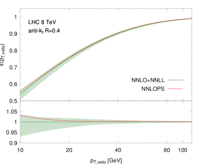
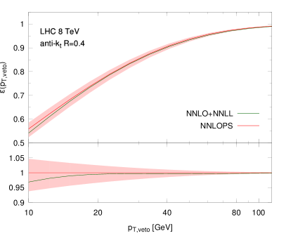
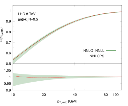
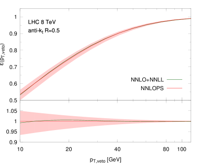
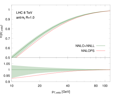
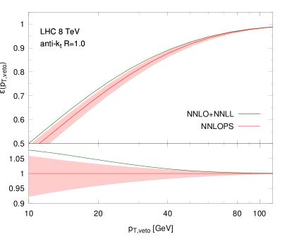
Figure 4.9: Comparison of NNLOPS (red) prediction and NNLO+NNLL resummation (green) for the jet-veto efficiency for $Z$ production at 8 TeV LHC for three different values of the jet-radius. The NNLOPS prediction is shown at parton level with parton showering performed with PYTHIA8.

Here results have been obtained for the LHC at 8 TeV, using the anti-$k_{t}$ algorithm to construct jets. We restrict ourselves to show NNLOPS results obtained with PYTHIA8. Analytically resummed results have been obtained using JetVHeto [199], and have NNLL+NNLO accuracy. The JetVHeto results have been obtained using its default setting, i.e. using as a central value for the renormalisation, factorisation and resummation scale $M_{\scriptscriptstyle\mathrm{Z}}/2$.

As is recommended in Reference [199], for the JetVHeto results we have obtained the uncertainty band as an envelope of eleven curves: we have varied the renormalisation and factorisation scales independently giving rise to the usual 7-scale choices, additionally, for central renormalisation and factorisation scales we have varied the resummation scale up and down by a factor 2 and looked at two different additional schemes to compute the efficiency.

We observe a very good agreement between the two approaches for $R=0.4$ and $0.5$, whereas for $R=1$ differences are more marked. Few comments are in order here: first, the pattern shown in the plots is consistent with what was already observed in the Higgs case (Figure 7 of Reference [113]), namely differences up to few percents, and good band overlap, for smaller values of $R$, and larger differences for $R=1$. For very large values of $R$, the leading-jet momentum will balance against the transverse momentum of the vector boson. Given what we observed for $p_{\scriptscriptstyle\mathrm{T,Z}}$, it is therefore no surprise that, when $R=1$, we have $\mathcal{O}(3-5)\%$ differences with respect to the resummed result for values of $p_{\mathrm{T,veto}}\sim 25-30\;\mathrm{GeV}$, as used currently by ATLAS and CMS in Higgs production.

4.3.3 Comparison to Data

In this section we compare our predictions with a number of available data from ATLAS, both for $Z$ and for $W$ production.

4.3.3.1 $Z$ Production

We show here a comparison to a number of measurements performed by ATLAS at 7 TeV [214, 215, 216]. ATLAS applied the following cuts: they consider the leptonic decay of the $Z$ boson to electrons or muons and require an electron (muon) and a positron (anti-muon) with $p_{\scriptscriptstyle\mathrm{T}}>20\;\mathrm{GeV}$ and rapidity $|y|<2.4$. The invariant mass of the di-lepton pair should lie in the window $66\;\mathrm{GeV}<m_{\mathrm{ll}}<116\;\mathrm{GeV}$.

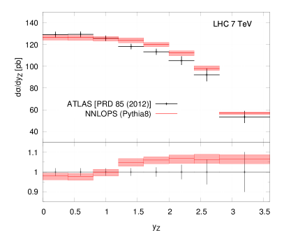
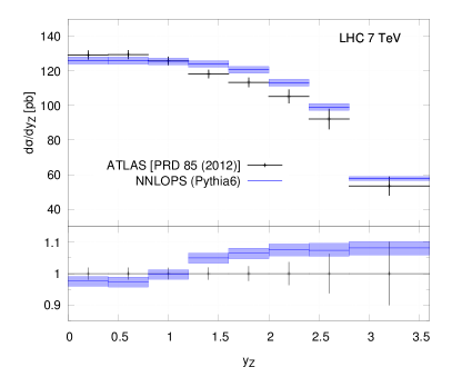
Figure 4.10: Comparison of NNLOPS prediction obtained with PYTHIA8 (left) and PYTHIA6 (right) to data (black) from Reference [214] for the $Z$ boson rapidity distribution at 7 TeV LHC.

We begin by showing in Figure 4.10 a comparison of NNLOPS results (with two versions of PYTHIA) to data from Reference [214] for the $Z$ boson rapidity distribution. As expected, our result displays a quite narrow uncertainty band, due to having included NNLO corrections. Since this is a fully inclusive observable, the absolute value of the cross-section and the size of the uncertainty band will be driven by the NNLO reweighting: hence, PYTHIA6 and PYTHIA8 results are almost indistinguishable, as expected. We also observe that we agree with data within the errors for central rapidities. At high rapidity, however, there seems to be a tension between data and our results. This discrepancy between data and pure NNLO was already observed in the original ATLAS paper, although the NNLO results shown in Reference [214] have a slightly larger uncertainty band since they also contain PDF uncertainties. We note that, at the moment, the dominant error is coming from data. In a more recent analysis of $13\;\mathrm{TeV}$ data [179] good agreement is found between data and POWHEG events, which makes us expect a similar agreement with our NNLOPS results.

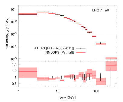
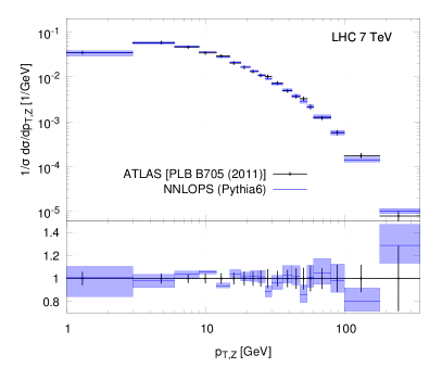
Figure 4.11: Comparison to data from Reference [215] for the $Z$ boson transverse distribution at 7 TeV LHC. Normalised data compared with NNLOPS showered with PYTHIA8 (left plot, red) and PYTHIA 6 (right plot, blue). Uncertainty bands for the theoretical predictions are obtained by first normalising all scale choices, as described in Section 4.3.2.1 and then taking the associated envelope of these normalised distributions.

In Figure 4.11 we now show the same comparison for the $Z$ boson transverse momentum against data from Reference [215]. In the left panel we use PYTHIA8 to shower events and in the right panel PYTHIA6. We see that there is very good agreement between our NNLOPS prediction over the whole $p_{\scriptscriptstyle\mathrm{T}}$ range. Only in the very first bin we observe a slight tension with data in the case of PYTHIA8, which can be due to a different modelling of non-perturbative effects. Given the fact that we use two different parton-showers, with different tunes (and even different PDFs for the tunes), an $\mathcal{O}(20\%)$ difference in the $1-3\;\mathrm{GeV}$ region can be expected. It is foreseeable that once a tuning of PYTHIA8 is done in conjunction with POWHEG, such differences will go away.

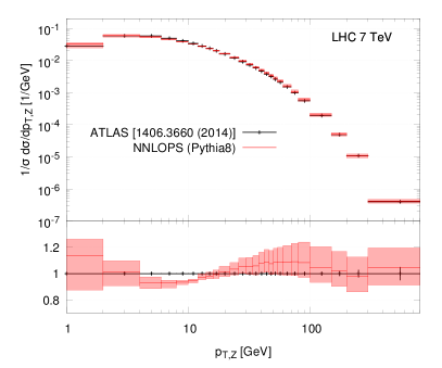
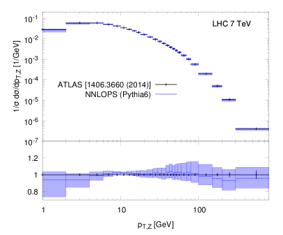
Figure 4.12: As in previous figure, but with more luminosity, thinner binning, and up to larger values of $p_{\scriptscriptstyle\mathrm{T,Z}}$. Data are now from taken from Reference [217].

Figure 4.12 shows again $p_{\scriptscriptstyle\mathrm{T,Z}}$, based now on $4.7\;\mathrm{fb}^{-1}$ of data from ATLAS [217]. Due to the thinner binning, it is now possible to appreciate clearly the differences between PYTHIA6 and PYTHIA8: the NNLOPS result obtained with PYTHIA6 shows a remarkable agreement with data across all the $p_{\scriptscriptstyle\mathrm{T,Z}}$ range, whereas with PYTHIA8 we can observe differences of up to 10% for $5\lesssim p_{\scriptscriptstyle\mathrm{T,Z}}\lesssim 100\;\mathrm{GeV}$. What we observe from these plots is consistent with Figure 4.11, the difference being that here the improved precision in data allows us to conclude that for the setups and tunes we are using, the best description is obtained when using PYTHIA6.

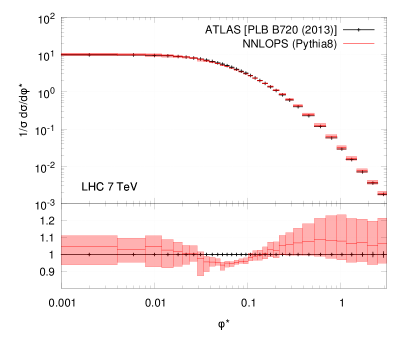
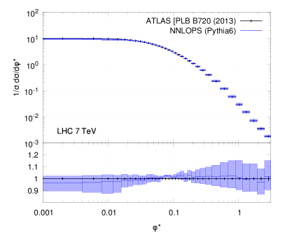
Figure 4.13: As in Figure 4.11 for the $\phi^{*}$ distribution in $Z$ boson production. Data taken from Reference [216].

Next, in Figure 4.13, we consider the comparison to data for the $\phi^{*}$ distribution. Although both our predictions are consistent with the ATLAS measurement, it is clear that events showered with PYTHIA6 agree better with data, whereas NNLOPS showered with PYTHIA8 has a slightly different shape, exhibiting a dip in the theory prediction compared with data, at around $\phi^{*}=0.06$. By comparing with our predictions before the inclusion of non-perturbative effects, we have checked that these effects play a sizeable role in the region below $\phi^{*}<0.1$, therefore it is not completely unexpected that PYTHIA6 and PYTHIA8 give slightly different shapes. The fact that non-perturbative effects introduce non-trivial changes on the shape of this distribution was also noted in Reference [198] (for predictions at the Tevatron). We also observe the same pattern shown in Reference [198], namely a moderate increase at $\phi^{*}\sim 0.05$ and a more pronounced decrease for very low values of $\phi^{*}$ when non-perturbative effects are included. Finally, it is worth mentioning that the results we have obtained (especially with PYTHIA6) clearly show a better agreement with data than what was found in Reference [215], where different tunes were used, both for PYTHIA6 and PYTHIA8. It is difficult to draw a solid conclusion, since in Reference [215] POWHEG-Z (as opposed to Zj-MiNLO) was used, and events were also reweighted using ResBos [218]. Nevertheless it seems clear that the best agreement are obtained when higher-order perturbative corrections are included and modern tunes are used.

4.3.3.2 $W$ Production

In this section we compare our predictions to results of References [219, 220], and in particular we use the combined decay of the $W$ to electrons and muons. The charged lepton is required to have $p_{\scriptscriptstyle\mathrm{T}}>20\;\mathrm{GeV}$ and rapidity $|y|<2.4$. The event must have a missing energy $p_{\mathrm{T},miss}>25\;\mathrm{GeV}$ and the transverse mass of the $W$ boson defined as $m_{\scriptscriptstyle\mathrm{T,W}}=\sqrt{2(p_{{\scriptscriptstyle\mathrm{T}},l}\,p_{{\scriptscriptstyle\mathrm{T}},\mathrm{miss}}-\vec{p}_{{\scriptscriptstyle\mathrm{T}},l}\,\cdot\vec{p}_{{\scriptscriptstyle\mathrm{T}},\mathrm{miss}})}$ must be above $40\;\mathrm{GeV}$. As was the case for the $Z$ studies, ATLAS only provides normalised distributions for the standard observables we will show here.

We start by showing in Figure 4.14 the transverse momentum of the $W$ boson, $p_{\scriptscriptstyle\mathrm{T,W}}$. As expected, differences in the parton shower algorithm only play a visible role in the small $p_{\scriptscriptstyle\mathrm{T}}$ region, where minor differences between PYTHIA6 and PYTHIA8 can be observed. For high $p_{\scriptscriptstyle\mathrm{T,W}}$, the two predictions are consistent with each other, and agree quite well with data.

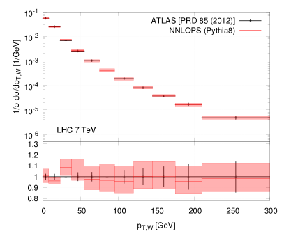
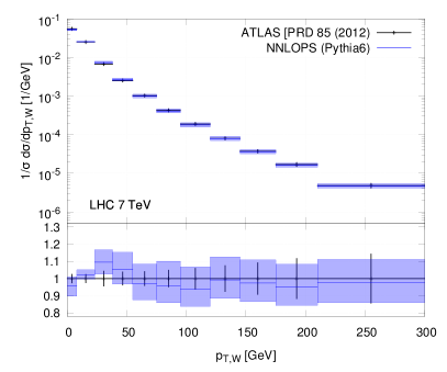
Figure 4.14: Comparison of NNLOPS prediction (red) to data (black) from Reference [219] for the $W$ boson $p_{\scriptscriptstyle\mathrm{T,W}}$ distribution, using PYTHIA8 (left) and PYTHIA6 (right).

We also compared our predictions with the analysis performed by the ATLAS collaboration in Reference [220]. We show results for $k_{\scriptscriptstyle\mathrm{T}}$-splitting scales in $W+$jets events. These observables are defined as the smallest distances found by the (inclusive) $k_{\scriptscriptstyle\mathrm{T}}$-algorithm at each step in the clustering sequence. The splitting scale $d_{k}$ is the smallest among all distances found by the algorithm when going from $(k+1)$ to $k$ objects. Therefore $\sqrt{d_{0}}$ corresponds to the transverse momentum of the leading jet, whereas $\sqrt{d_{1}}$ is the smallest distance among pseudo-jets when clustering from $2$ to $1$ jet:

$$d_{1}=\min(d_{1B},d_{2B},d_{12})\,,$$ (4.39)

where

$$d_{iB} = p^{2}_{\scriptscriptstyle\mathrm{T,i}}\,,$$

$$d_{ij} = \min(p^{2}_{\scriptscriptstyle\mathrm{T,i}},p^{2}_{\scriptscriptstyle\mathrm{T,j}})\frac{(\Delta R_{ij})^{2}}{R^{2}}\,,$$ (4.40)

are the usual distances used in the $k_{\scriptscriptstyle\mathrm{T}}$-algorithm. Among other reasons, these observables are interesting because they can be used as a probe of the details of matching and merging schemes. Due to the underlying Zj-MiNLO simulation, our NNLOPS prediction is NLO accurate for large values of $p_{\scriptscriptstyle\mathrm{T,j_{1}}}$, and it is at least LL accurate in describing the $1\to 0$ jet transition, which is measured in the $d_{0}$ distribution. The second jet spectrum and the $2\to 1$ jet transition (which is encapsulated in $d_{1}$) are instead described at LO+LL, due to the underlying POWHEG simulation. Since the definition of $d_{1}$ contains $d_{12}$, this observable is a measure of the internal structure of the first jet, and not only of the second jet transverse momentum.

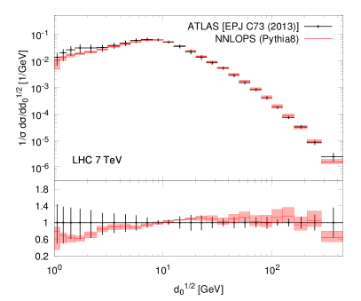
Figure 4.15: Comparison of NNLOPS prediction (red) to 7 TeV LHC data (black) from Reference [220] for the $W$ boson $k_{\scriptscriptstyle\mathrm{T}}$ splitting scale $\sqrt{d_{0}}$ as defined in the text using PYTHIA8 (left) and PYTHIA6 (right).

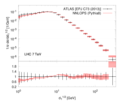
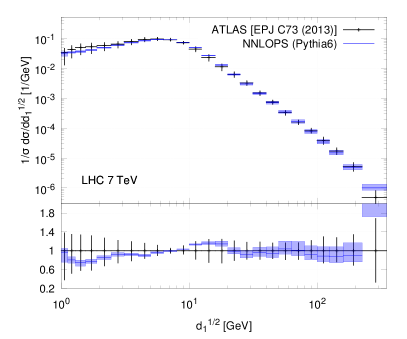
Figure 4.16: Comparison to 7 TeV LHC data from Reference [220] for the $W$ boson $k_{\scriptscriptstyle\mathrm{T}}$ splitting scale $\sqrt{d_{1}}$ as defined in Equation 4.39 using PYTHIA8 (left) and PYTHIA6 (right).

In Figures 4.15 and 4.16 we show our NNLOPS predictions against ATLAS data, using as jet radius $R=0.6$. We find good agreement, especially when $\sqrt{d_{i}}>10\;\mathrm{GeV}$. Below this value, we are still compatible with the experimental uncertainty bands, although we are systematically lower than data. Once more, one should consider that the region below $5-10\;\mathrm{GeV}$ will be affected also by non-perturbative effects. For large values of $d_{i}$ we are instead sensitive to the level of accuracy that we reach in describing hard emissions. In this respect, it is no surprise that we have a better agreement with data than the POWHEG results shown in Reference [220], where $d_{1}$ is poorly described since the second emission is only described in the shower approximation. NLO corrections to the $W+1$ jet region are included in the NNLOPS simulation, and are very likely the reason why we have a description of $d_{0}$ that is better than what was observed in Reference [220].

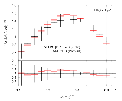
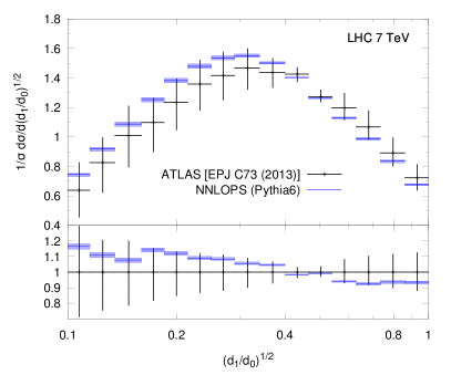
Figure 4.17: Comparison to 7 TeV LHC data from Reference [220] for the $W$ boson ratio of the $k_{\scriptscriptstyle\mathrm{T}}$ splitting scales $\sqrt{d_{0}}$ and $\sqrt{d_{1}}$ using PYTHIA8 (left) and PYTHIA6 (right).

Finally in Figure 4.17 we show the distribution for the ratio $d_{1}/d_{0}$, for events with $\sqrt{d_{0}}>20\;\mathrm{GeV}$. Due to the ratio nature of this quantity, a simultaneous over- or underestimation in predicting $d_{1}$ and $d_{0}$ should be partially compensated when plotting $d_{1}/d_{0}$. It is therefore no surprise that the agreement with data is better than in Figures 4.15 and 4.16.

4.3.3.3 $W$ and $Z$ Polarisation

Recently both ATLAS [221] and CMS [222] have published results on the polarisation of the $W$ boson at 7 TeV confirming the Standard Model prediction that $W$ bosons are mostly left-handed in $pp$ collisions at large transverse momenta [223]. Knowledge about the $W$ boson polarisation is important, as it provides a discriminant in searches for new physics.

We first very briefly review how to measure the polarisation in terms of angular coefficients but refer the reader to the literature for a complete description of the topic [223, 224, 225, 226, 227, 228, 229, 230]. Here we will follow the derivation of [223]. We then continue to compare ATLAS data [221] to our NNLOPS results for the $W$ boson polarisation and present predictions for the angular coefficients for the $Z$ boson at 8 TeV.

The vector boson cross-section can be expanded in terms of $\cos{\theta^{*}}$ and $\phi^{*}$ as

$$\frac{1}{\sigma}\frac{d\sigma}{d(\cos{\theta^{*}})d\phi^{*}}= \frac{3}{16\pi}\Bigl{[}(1+\cos^{2}\theta^{*})+A_{0}\frac{1}{2}(1-3\cos^{2}{\theta^{*}})+A_{1}\sin 2\theta^{*}\cos\phi^{*}$$

$$+A_{2}\frac{1}{2}\sin^{2}\theta^{*}\cos 2\phi^{*}+A_{3}\sin\theta^{*}\cos\phi^{*}+A_{4}\cos\theta^{*}$$

$$+A_{5}\sin\theta^{*}\sin\phi^{*}+A_{6}\sin 2\theta^{*}\sin\phi^{*}+A_{7}\sin^{2}\theta^{*}\sin 2\phi^{*}\Bigr{]}\,,$$ (4.41)

where the polar angle $\theta^{*}$ and the azimuthal angle $\phi^{*}$ are defined in some particular rest frame of the dilepton system. Here we will make use of two different frames, the Collins-Soper frame [224] for the $Z$ boson and the helicity frame for the $W$ boson defined as the dilepton rest frame with the z-axis pointing along the direction of flight of the $W$ boson in the lab frame. The cross-section can be differential in any quantity that does not depend on the individual lepton kinematics. The angular coefficients can then be expressed in terms of expectation values defined as

$$<f(\theta^{*},\phi^{*})>=\int_{-1}^{1}d(\cos\theta^{*})\int_{0}^{2\pi}d\phi^{*}\frac{1}{\sigma}\frac{d\sigma}{d(\cos{\theta^{*}})d\phi^{*}}f(\theta^{*},\phi^{*})$$ (4.42)

by

$$A_{0} =4-<10\cos^{2}\theta^{*}>, \quad A_{1}= <5\sin 2\theta^{*}\cos\phi^{*}>, \quad A_{2}= <10\sin^{2}\theta^{*}\cos 2\phi^{*}>\,,$$

$$A_{3} =<4\sin\theta^{*}\cos\phi^{*}>, A_{4}= <4\cos\theta^{*}>,\phantom{\sin\theta^{*}} A_{5}= <5\sin^{2}\theta^{*}\sin 2\phi^{*}>\,,$$

$$A_{6} =<5\sin 2\theta^{*}\sin\phi^{*}>, A_{7}= <4\sin\theta^{*}\sin\phi^{*}>.$$ (4.43)

For both $W$ and $Z$ production it is known that at $\mathcal{O}(\alpha_{s})$ $A_{5}=A_{6}=A_{7}=0$. Here we have checked that with 20 million $Z$ events at 8 TeV, and using only a cut on the invariant mass of $66\;\mathrm{GeV}<m_{ll}<116\;\mathrm{GeV}$, the coefficients do not deviate significantly from zero and we have therefore chosen not to show them. It is also interesting to notice that as a consequence of the spin-1 structure of the gluon, the Lam-Tung relation $A_{0}=A_{2}$ holds at LO [231]. As we will see, the deviations from this lowest-order result can become quite large, $\mathcal{O}(20\%)$, in the $p_{\scriptscriptstyle\mathrm{T,Z}}>10\;\mathrm{GeV}$ region. From the angular coefficients we then define the left, $f_{L}$, right, $f_{R}$, and longitudinal, $f_{0}$, polarisation fractions of the $W^{\pm}$ as

$$f_{L}=\frac{1}{4}(2-A_{0}\mp A_{4}),\quad f_{R}=\frac{1}{4}(2-A_{0}\pm A_{4}),\quad f_{0}=\frac{1}{2}A_{0}\,.$$ (4.44)

It is clear from these equations that the polarisation fractions are normalised such that $f_{L}+f_{R}+f_{0}=1$ and it is therefore sufficient to show results for $f_{L}-f_{R}$ and $f_{0}$. In this way we also separate the $A_{0}$ and $A_{4}$ dependence. In Table 4.1 we show our prediction for $f_{L}-f_{R}$ and $f_{0}$ for combined $W^{+}$ and $W^{-}$ production at 7 TeV compared with ATLAS data [221] for two different $p_{\scriptscriptstyle\mathrm{T}}$ regions. We find good agreement between the data and predictions - three of them at the $1\sigma$ level and at the $2\sigma$ level for $f_{L}-f_{R}$ in the low $p_{\scriptscriptstyle\mathrm{T}}$ range. It should be noted that the measurements are dominated by systematic uncertainties.

	$35\;\mathrm{GeV}<p_{\scriptscriptstyle\mathrm{T,W}}<50\;\mathrm{GeV}$		$p_{\scriptscriptstyle\mathrm{T,W}}>50\;\mathrm{GeV}$
	$f_{L}-f_{R}$	$f_{0}$	$f_{L}-f_{R}$	$f_{0}$
Data	$0.238\pm 0.02\pm 0.034$	$0.219\pm 0.033\pm 0.134$	$0.252\pm 0.017\pm 0.034$	$0.127\pm 0.03\pm 0.108$
NNLOPS	$0.317\pm 0.002$	$0.198\pm 0.004$	$0.289\pm 0.004$	$0.214\pm 0.009$

Table 4.1: A comparison between combined $W^{+}$ and $W^{-}$ at 7 TeV ATLAS data [221] and our NNLOPS prediction for $f_{L}-f_{R}$ and $f_{0}$ as defined in Equation 4.44 and. For data the first uncertainty is statistical and the second one systematic. For the theoretical prediction the error is purely statistical. Except for the $p_{\scriptscriptstyle\mathrm{T,W}}$ cut the only cut imposed on the theoretical prediction is a transverse mass cut of $m_{\scriptscriptstyle\mathrm{T,W}}>40\;\mathrm{GeV}$. The data and predictions are in good agreement.

When this work was carried out, there was no public measurement for the angular coefficients for the $Z$ boson in $pp$ collisions. Previously measurements of $A_{0},A_{2},A_{3}$ and $A_{4}$ in $p\bar{p}$ collisions had been published by the CDF collaboration [232] and very recently an analysis was published by ATLAS [211] of the angular coefficients in $Z$-boson events at $8\;\mathrm{TeV}$. This analysis finds significant deviations in $A_{0}-A_{2}$ from theoretical predictions obtained with the Zj-MiNLO generator. We here present our predictions for the angular coefficients as defined in Equation 4.43, as a function of the boson transverse momentum at $8\;\mathrm{TeV}$. We impose an invariant mass cut of $66\;\mathrm{GeV}<m_{ll}<116\;\mathrm{GeV}$, but beyond that no other cuts are imposed. In the left panel of Figure 4.18 we plot $A_{0}$ (red) and $A_{2}$ (blue) along with the difference $A_{0}-A_{2}$, while in the right panel we plot $A_{1},A_{3}$ and $A_{4}$.

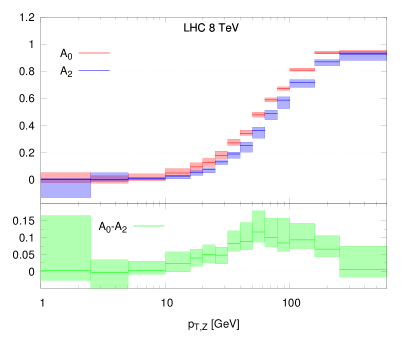
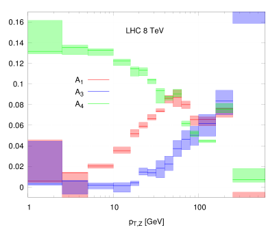
Figure 4.18: Predictions for angular coefficients Equation 4.43 in the Collins-Soper frame for $Z$ production at 8 TeV. In the left panel we show $A_{0}$ (red) and $A_{2}$ (blue) along with the difference $A_{0}-A_{2}$ (green) and in the right panel we plot $A_{1}$ (red), $A_{3}$ (blue) and $A_{4}$ (green). The only cut imposed is on the invariant mass of the dilepton system, $66\;\mathrm{GeV}<m_{ll}<116\;\mathrm{GeV}$.

For the two coefficients $A_{0}$ and $A_{2}$ we find that they are in very good agreement for low transverse momentum, $p_{\scriptscriptstyle\mathrm{T,Z}}<10\;\mathrm{GeV}$. For higher transverse momenta deviations start to appear peaking around $60\;\mathrm{GeV}$. For the three other coefficients, we observe that the $p_{\scriptscriptstyle\mathrm{T}}$ dependence is strongest for larger transverse momenta. We can define polarisation fractions for the $Z$ boson analogously to those defined in Equation 4.44 by [233]

$$f_{L}=\frac{1}{4}(2-A_{0}-\alpha A_{4})\,,\quad f_{R}=\frac{1}{4}(2-A_{0}+\alpha A_{4})\,,\quad f_{0}=\frac{1}{2}A_{0}\,,$$ (4.45)

where $\alpha=\frac{c_{L}^{2}-c_{R}^{2}}{c_{L}^{2}+c_{R}^{2}}$, $c_{L}$ is the coupling to the left-handed lepton and $c_{R}$ is the coupling to the right-handed lepton. As for the $W$ boson these are normalised such that $f_{L}+f_{R}+f_{0}=1$ and we have in this case that $f_{L}-f_{R}=-\frac{1}{2}\alpha A_{4}$. Using $c_{L}=\sin^{2}\theta_{W}-\frac{1}{2}$ and $c_{R}=\sin^{2}\theta_{W}$ we get $\alpha\approx 0.032$. Comparing with Figure 4.18 we see that at low $p_{\scriptscriptstyle\mathrm{T}}$ the longitudinal polarisation of the $Z$ boson, $f_{0}$, is highly suppressed and it is produced almost equally between the left- and right-handed polarisation. For high $p_{\scriptscriptstyle\mathrm{T}}$ the longitudinal polarisation starts to dominate.

4.4 Conclusions

In this chapter we reviewed the MiNLO procedure and described how a Vj-MiNLO generator can be upgraded through a reweighting procedure to exhibit NNLO⁽⁰⁾ accuracy. At the core of this method lies the fact that the Zj-MiNLO and Wj-MiNLO simulations achieve NLO accuracy also for fully inclusive distributions, i.e. once the jet is integrated out. In the case of Higgs production considered recently in Reference [113], it was enough to rescale the NLOPS results to reproduce the NNLO Higgs rapidity spectrum, thereby achieving NNLOPS accuracy. In the present case instead, to properly take into account the decay of the boson to leptons, NNLOPS accuracy is reached by performing a three-dimensional rescaling of the events generated by Zj-MiNLO and Wj-MiNLO using NNLO distributions as computed, for instance, with DYNNLO. This implies that the calculation is numerically more intensive.

We have validated our procedure by considering observables typically used to study Drell-Yan processes. We have found extremely good agreement with NNLO results for observables fully inclusive over QCD radiation, and all the features expected in a computation matched with parton showers for more exclusive observables. We have also compared our NNLOPS predictions to state-of-the-art analytic resummation for observables sensitive to soft-collinear QCD radiation, which are not described accurately by a fixed-order NNLO calculation. Despite the fact that the logarithmic accuracy of our simulation cannot be claimed to reach the same precision as these analytic resummations, we have found reasonably good agreement for the vector boson transverse momentum. Slightly more pronounced discrepancies were observed for $\phi^{*}$ and for the jet-veto efficiency for large values of the jet radius $R$.

We have also compared with a number of available experimental results, not only for fully inclusive observables but also for $\phi^{*}$, the transverse momentum of the vector boson, as well as $k_{\scriptscriptstyle\mathrm{T}}$ splitting scales. The successful outcome of these comparisons is an indication that our computation can be used as a state of the art prediction for future studies where a simultaneous inclusion of NNLO corrections and parton shower effects are needed. We have also illustrated how our generator can be used to study the polarisation of $W$ and $Z$ bosons produced in Drell-Yan events.

We finally remark that we did not include in this work electroweak corrections. These corrections are known exactly at one loop [186, 189] and can be included, at ${\mathcal{O}}(\alpha_{ew})$ either additively or multiplicative on top of the QCD corrections included here. Version 3 of the program FEWZ [193] includes directly both EW and QCD corrections, however we could not use it to generate the three dimensional distributions needed here.

Chapter 5 Final Remarks

In this thesis we have presented a number of recent results in precision QCD, spanning from fixed-order differential NNLO and inclusive N³LO calculations to the matching of NLO and NNLO calculations with parton showers. Given the vast amount of data which the LHC is currently gathering, these types of calculations will soon become crucial in determining the fate of the Standard Model. In the absence of any new resonances or clear indications of physics beyond the Standard Model, our ability to disentangle the truth from data will be limited by the accuracy of our theoretical predictions. Several complementary techniques exist to improve the reliability of these predictions of which we have investigated a few here.

Except for the POWHEG method presented in Chapter 3, which is extremely versatile, the methods we have studied here all have their limitations. The MiNLO procedure can in principle be applied to any final state, but the reweighting procedure that we introduced in Chapter 4 becomes numerically unfeasible quickly as the number of external legs grow. However, the success of the method indicates that we are on the right track, and that we may expect to formulate a more general NNLOPS method along the lines of POWHEG in the future. The calculation of N³LO accurate inclusive VBF Higgs production presented in Chapter 1, was based on an old observation that the VBF process factorises and can be described by the proton structure functions. Although this point-of-view is not exact beyond NLO, it is accurate to the percent level, and most of the contributions neglected by the approximation have been calculated fully and could in principle be included. These are definitely needed as soon as one goes beyond NNLO, as the N³LO corrections and associated scale uncertainties are at the permille level. Although permille corrections are not phenomenologically interesting (yet), their smallness demonstrate the excellent convergence exhibited by perturbative QCD. In addition to that, our knowledge of processes at N³LO will in turn feed into the determination of PDFs, thereby improving our modelling of the proton. Besides the inherent approximation of the structure function approach, it has the further limitation of not being able to describe the full final state due to the implicit integration over hadronic final states. This limitation we eliminated in Chapter 2 by introducing the “projection-to-Born” method, effectively undoing the aforementioned integration. The “projection-to-Born” method is very general in the sense that it can be applied at any perturbative order. However, it only applies to processes for which one can assign Born-like kinematics, and therefore it will be interesting to see how applicable the method is in the future. At this point it has already been used in the calculation of NNLO t-channel single top-quark production [234] in addition to the calculation presented here.

Although QCD has been around for almost half a century, and its phenomenology is well established, we are still far from being done investigating the consequences of the strong interactions in particle collisions. Even state of the art calculations can at best claim an accuracy of a few percent when one takes into account the effects of physics from PDFs, parton showering, non-perturbative QCD, and EW effect. It is therefore not a bold claim to say that the era of precision QCD has only just begun, and that it will be around for a very long time to come.

References

- Cacciari et al. [2015] Matteo Cacciari, Frédéric A. Dreyer, Alexander Karlberg, Gavin P. Salam, and Giulia Zanderighi. Fully Differential Vector-Boson-Fusion Higgs Production at Next-to-Next-to-Leading Order. Phys. Rev. Lett., 115(8):082002, 2015. 10.1103/PhysRevLett.115.082002.
- Dreyer and Karlberg [2016] Frédéric A. Dreyer and Alexander Karlberg. Vector-Boson Fusion Higgs Production at Three Loops in QCD. Phys. Rev. Lett., 117(7):072001, 2016. 10.1103/PhysRevLett.117.072001.
- Contino et al. [2016] R. Contino et al. Physics at a 100 TeV pp collider: Higgs and EW symmetry breaking studies. 2016. URL http://cds.cern.ch/record/2195530.
- LHC Higgs Cross Section Working Group and et al [Eds.] LHC Higgs Cross Section Working Group and Anastasiou C. et al (Eds.). Handbook of LHC Higgs Cross Sections: 4. Deciphering the nature of the Higgs sector. (Forthcoming), CERN, Geneva, 2016.
- Jäger et al. [2014a] Barbara Jäger, Alexander Karlberg, and Giulia Zanderighi. Electroweak production in the Standard Model and beyond in the POWHEG-BOX V2. JHEP, 03:141, 2014a. 10.1007/JHEP03(2014)141.
- Karlberg et al. [2014] Alexander Karlberg, Emanuele Re, and Giulia Zanderighi. NNLOPS accurate Drell-Yan production. JHEP, 09:134, 2014. 10.1007/JHEP09(2014)134.
- Alioli et al. [2016] S. Alioli et al. Precision Studies of Observables in pp->W->l nu and pp->gamma,Z->l+l- processes at the LHC. 2016. URL http://cds.cern.ch/record/2159869.
- Aad et al. [2012a] Georges Aad et al. Observation of a new particle in the search for the Standard Model Higgs boson with the ATLAS detector at the LHC. Phys.Lett., B716:1–29, 2012a. 10.1016/j.physletb.2012.08.020.
- Chatrchyan et al. [2012] Serguei Chatrchyan et al. Observation of a new boson at a mass of 125 GeV with the CMS experiment at the LHC. Phys.Lett., B716:30–61, 2012. 10.1016/j.physletb.2012.08.021.
- Khachatryan et al. [2015a] Vardan Khachatryan et al. Search for the standard model Higgs boson produced through vector boson fusion and decaying to . Phys. Rev., D92(3):032008, 2015a. 10.1103/PhysRevD.92.032008.
- LHC Higgs Cross Section Working Group et al. [CERN, Geneva, 2011] LHC Higgs Cross Section Working Group, S. Dittmaier, C. Mariotti, G. Passarino, and R. Tanaka (Eds.). Handbook of LHC Higgs Cross Sections: 1. Inclusive Observables. CERN-2011-002, CERN, Geneva, 2011. 10.5170/CERN-2011-002.
- Jones and Petcov [1979] D. R. T. Jones and S. T. Petcov. Heavy Higgs Bosons at LEP. Phys. Lett., B84:440–444, 1979. 10.1016/0370-2693(79)91234-6.
- LHC Higgs Cross Section Working Group et al. [CERN, Geneva, 2012] LHC Higgs Cross Section Working Group, S. Dittmaier, C. Mariotti, G. Passarino, and R. Tanaka (Eds.). Handbook of LHC Higgs Cross Sections: 2. Differential Distributions. CERN-2012-002, CERN, Geneva, 2012. 10.5170/CERN-2012-002.
- LHC Higgs Cross Section Working Group et al. [CERN, Geneva, 2013] LHC Higgs Cross Section Working Group, S. Heinemeyer, C. Mariotti, G. Passarino, and R. Tanaka (Eds.). Handbook of LHC Higgs Cross Sections: 3. Higgs Properties. CERN-2013-004, CERN, Geneva, 2013. 10.5170/CERN-2013-004.
- collaboration [2015] The ATLAS collaboration. Search for an Invisibly Decaying Higgs Boson Produced via Vector Boson Fusion in Collisions at TeV using the ATLAS Detector at the LHC. 2015. URL http://cds.cern.ch/record/2002121.
- Collaboration [2015] CMS Collaboration. Search for invisible decays of Higgs bosons in the vector boson fusion production mode. 2015. URL http://cds.cern.ch/record/2007270.
- Plehn et al. [2002] Tilman Plehn, David L. Rainwater, and Dieter Zeppenfeld. Determining the structure of Higgs couplings at the LHC. Phys. Rev. Lett., 88:051801, 2002. 10.1103/PhysRevLett.88.051801.
- Zeppenfeld et al. [2000] D. Zeppenfeld, R. Kinnunen, A. Nikitenko, and E. Richter-Was. Measuring Higgs boson couplings at the CERN LHC. Phys. Rev., D62:013009, 2000. 10.1103/PhysRevD.62.013009.
- Aad et al. [2016a] Georges Aad et al. Measurements of the Higgs boson production and decay rates and constraints on its couplings from a combined ATLAS and CMS analysis of the LHC pp collision data at and 8 TeV. JHEP, 08:045, 2016a. 10.1007/JHEP08(2016)045.
- Han et al. [1992] Tao Han, G. Valencia, and S. Willenbrock. Structure function approach to vector boson scattering in p p collisions. Phys. Rev. Lett., 69:3274–3277, 1992. 10.1103/PhysRevLett.69.3274.
- Bolzoni et al. [2010] Paolo Bolzoni, Fabio Maltoni, Sven-Olaf Moch, and Marco Zaro. Higgs production via vector-boson fusion at NNLO in QCD. Phys. Rev. Lett., 105:011801, 2010. 10.1103/PhysRevLett.105.011801.
- Bolzoni et al. [2012] Paolo Bolzoni, Fabio Maltoni, Sven-Olaf Moch, and Marco Zaro. Vector boson fusion at NNLO in QCD: SM Higgs and beyond. Phys. Rev., D85:035002, 2012. 10.1103/PhysRevD.85.035002.
- Zaro [2013] Marco Zaro. Accurate predictions for Higgs production at the LHC : the VBF channel. PhD thesis, Louvain U., CP3, 2013. URL http://hdl.handle.net/2078.1/133425.
- Anastasiou et al. [2015] Charalampos Anastasiou, Claude Duhr, Falko Dulat, Franz Herzog, and Bernhard Mistlberger. Higgs Boson Gluon-Fusion Production in QCD at Three Loops. Phys. Rev. Lett., 114:212001, 2015. 10.1103/PhysRevLett.114.212001.
- Anastasiou et al. [2016] Charalampos Anastasiou, Claude Duhr, Falko Dulat, Elisabetta Furlan, Thomas Gehrmann, Franz Herzog, Achilleas Lazopoulos, and Bernhard Mistlberger. High precision determination of the gluon fusion Higgs boson cross-section at the LHC. JHEP, 05:058, 2016. 10.1007/JHEP05(2016)058.
- Forte et al. [2014] Stefano Forte, Andrea Isgrò, and Gherardo Vita. Do we need N3LO Parton Distributions? Phys. Lett., B731:136–140, 2014. 10.1016/j.physletb.2014.02.027.
- Ellis et al. [1996] R. Keith Ellis, W. James Stirling, and B. R. Webber. QCD and collider physics. Camb. Monogr. Part. Phys. Nucl. Phys. Cosmol., 8:1–435, 1996. URL http://www-spires.fnal.gov/spires/find/books/www?cl=QC793.3.Q35E44::1996.
- Moch et al. [2008] S. Moch, M. Rogal, and A. Vogt. Differences between charged-current coefficient functions. Nucl. Phys., B790:317–335, 2008. 10.1016/j.nuclphysb.2007.09.022.
- Davies et al. [2016] J. Davies, A. Vogt, S. Moch, and J. A. M. Vermaseren. Non-singlet coefficient functions for charged-current deep-inelastic scattering to the third order in QCD. In Proceedings, 24th International Workshop on Deep-Inelastic Scattering and Related Subjects (DIS 2016), 2016. URL http://inspirehep.net/record/1472971/files/arXiv:1606.08907.pdf.
- Ruijl et al. [2016] B. Ruijl, T. Ueda, J. A. M. Vermaseren, J. Davies, and A. Vogt. First Forcer results on deep-inelastic scattering and related quantities. In 13th DESY Workshop on Elementary Particle Physics: Loops and Legs in Quantum Field Theory (LL2016) Leipzig, Germany, April 24-29, 2016, 2016. URL http://inspirehep.net/record/1465859/files/arXiv:1605.08408.pdf.
- Vermaseren et al. [2005] J. A. M. Vermaseren, A. Vogt, and S. Moch. The Third-order QCD corrections to deep-inelastic scattering by photon exchange. Nucl. Phys., B724:3–182, 2005. 10.1016/j.nuclphysb.2005.06.020.
- Furmanski and Petronzio [1982] W. Furmanski and R. Petronzio. Lepton - Hadron Processes Beyond Leading Order in Quantum Chromodynamics. Z. Phys., C11:293, 1982. 10.1007/BF01578280.
- van Neerven and Vogt [2000a] W. L. van Neerven and A. Vogt. NNLO evolution of deep inelastic structure functions: The Singlet case. Nucl. Phys., B588:345–373, 2000a. 10.1016/S0550-3213(00)00480-6.
- Buehler and Lazopoulos [2013] Stephan Buehler and Achilleas Lazopoulos. Scale dependence and collinear subtraction terms for Higgs production in gluon fusion at N3LO. JHEP, 10:096, 2013. 10.1007/JHEP10(2013)096.
- Politzer [1973] H. David Politzer. Reliable Perturbative Results for Strong Interactions? Phys. Rev. Lett., 30:1346–1349, 1973. 10.1103/PhysRevLett.30.1346.
- Gross and Wilczek [1973] David J. Gross and Frank Wilczek. Ultraviolet Behavior of Nonabelian Gauge Theories. Phys. Rev. Lett., 30:1343–1346, 1973. 10.1103/PhysRevLett.30.1343.
- Caswell [1974] William E. Caswell. Asymptotic Behavior of Nonabelian Gauge Theories to Two Loop Order. Phys. Rev. Lett., 33:244, 1974. 10.1103/PhysRevLett.33.244.
- Tarasov et al. [1980] O. V. Tarasov, A. A. Vladimirov, and A. Yu. Zharkov. The Gell-Mann-Low Function of QCD in the Three Loop Approximation. Phys. Lett., B93:429–432, 1980. 10.1016/0370-2693(80)90358-5.
- Larin and Vermaseren [1993] S. A. Larin and J. A. M. Vermaseren. The Three loop QCD Beta function and anomalous dimensions. Phys. Lett., B303:334–336, 1993. 10.1016/0370-2693(93)91441-O.
- Lipatov [1975] L. N. Lipatov. The parton model and perturbation theory. Sov. J. Nucl. Phys., 20:94–102, 1975. [Yad. Fiz.20,181(1974)].
- Gribov and Lipatov [1972] V. N. Gribov and L. N. Lipatov. Deep inelastic e p scattering in perturbation theory. Sov. J. Nucl. Phys., 15:438–450, 1972. [Yad. Fiz.15,781(1972)].
- Altarelli and Parisi [1977] Guido Altarelli and G. Parisi. Asymptotic Freedom in Parton Language. Nucl. Phys., B126:298–318, 1977. 10.1016/0550-3213(77)90384-4.
- Dokshitzer [1977] Yuri L. Dokshitzer. Calculation of the Structure Functions for Deep Inelastic Scattering and e+ e- Annihilation by Perturbation Theory in Quantum Chromodynamics. Sov. Phys. JETP, 46:641–653, 1977. [Zh. Eksp. Teor. Fiz.73,1216(1977)].
- Vogt et al. [2004] A. Vogt, S. Moch, and J. A. M. Vermaseren. The Three-loop splitting functions in QCD: The Singlet case. Nucl. Phys., B691:129–181, 2004. 10.1016/j.nuclphysb.2004.04.024.
- Moch et al. [2004] S. Moch, J.A.M. Vermaseren, and A. Vogt. The Three loop splitting functions in QCD: The Nonsinglet case. Nucl.Phys., B688:101–134, 2004. 10.1016/j.nuclphysb.2004.03.030.
- Butterworth et al. [2016] Jon Butterworth et al. PDF4LHC recommendations for LHC Run II. J. Phys., G43:023001, 2016. 10.1088/0954-3899/43/2/023001.
- Nason and Oleari [2010] Paolo Nason and Carlo Oleari. NLO Higgs boson production via vector-boson fusion matched with shower in POWHEG. JHEP, 02:037, 2010. 10.1007/JHEP02(2010)037.
- Sanchez Guillen et al. [1991] J. Sanchez Guillen, J. Miramontes, M. Miramontes, G. Parente, and O. A. Sampayo. Next-to-leading order analysis of the deep inelastic R = sigma-L / sigma-total. Nucl. Phys., B353:337–345, 1991. 10.1016/0550-3213(91)90340-4.
- van Neerven and Zijlstra [1991] W. L. van Neerven and E. B. Zijlstra. Order alpha-s**2 contributions to the deep inelastic Wilson coefficient. Phys. Lett., B272:127–133, 1991. 10.1016/0370-2693(91)91024-P.
- Zijlstra and van Neerven [1992a] E. B. Zijlstra and W. L. van Neerven. Order alpha-s**2 QCD corrections to the deep inelastic proton structure functions F2 and F(L). Nucl. Phys., B383:525–574, 1992a. 10.1016/0550-3213(92)90087-R.
- Zijlstra and van Neerven [1992b] E. B. Zijlstra and W. L. van Neerven. Order alpha-s**2 correction to the structure function F3 (x, Q**2) in deep inelastic neutrino - hadron scattering. Phys. Lett., B297:377–384, 1992b. 10.1016/0370-2693(92)91277-G.
- van Neerven and Vogt [2000b] W. L. van Neerven and A. Vogt. NNLO evolution of deep inelastic structure functions: The Nonsinglet case. Nucl. Phys., B568:263–286, 2000b. 10.1016/S0550-3213(99)00668-9.
- Moch et al. [2005] S. Moch, J. A. M. Vermaseren, and A. Vogt. The Longitudinal structure function at the third order. Phys. Lett., B606:123–129, 2005. 10.1016/j.physletb.2004.11.063.
- Vogt et al. [2006] Andreas Vogt, Sven Moch, and Jos Vermaseren. Third-order QCD results on form factors and coefficient functions. Nucl. Phys. Proc. Suppl., 160:44–50, 2006. 10.1016/j.nuclphysbps.2006.09.101. [,44(2006)].
- Salam and Rojo [2009] Gavin P. Salam and Juan Rojo. A Higher Order Perturbative Parton Evolution Toolkit (HOPPET). Comput. Phys. Commun., 180:120–156, 2009. 10.1016/j.cpc.2008.08.010.
- Bertone et al. [2014] Valerio Bertone, Stefano Carrazza, and Juan Rojo. APFEL: A PDF Evolution Library with QED corrections. Comput. Phys. Commun., 185:1647–1668, 2014. 10.1016/j.cpc.2014.03.007.
- Dulat et al. [2016] Sayipjamal Dulat, Tie-Jiun Hou, Jun Gao, Marco Guzzi, Joey Huston, Pavel Nadolsky, Jon Pumplin, Carl Schmidt, Daniel Stump, and C. P. Yuan. New parton distribution functions from a global analysis of quantum chromodynamics. Phys. Rev., D93(3):033006, 2016. 10.1103/PhysRevD.93.033006.
- Harland-Lang et al. [2015] L. A. Harland-Lang, A. D. Martin, P. Motylinski, and R. S. Thorne. Parton distributions in the LHC era: MMHT 2014 PDFs. Eur. Phys. J., C75(5):204, 2015. 10.1140/epjc/s10052-015-3397-6.
- Ball et al. [2015] Richard D. Ball et al. Parton distributions for the LHC Run II. JHEP, 04:040, 2015. 10.1007/JHEP04(2015)040.
- van Ritbergen et al. [1997] T. van Ritbergen, J. A. M. Vermaseren, and S. A. Larin. The Four loop beta function in quantum chromodynamics. Phys. Lett., B400:379–384, 1997. 10.1016/S0370-2693(97)00370-5.
- Aad et al. [2015a] Georges Aad et al. Combined Measurement of the Higgs Boson Mass in Collisions at and 8 TeV with the ATLAS and CMS Experiments. Phys. Rev. Lett., 114:191803, 2015a. 10.1103/PhysRevLett.114.191803.
- Olive et al. [2014] K. A. Olive et al. Review of Particle Physics. Chin. Phys., C38:090001, 2014. 10.1088/1674-1137/38/9/090001.
- Ciccolini et al. [2008] Mariano Ciccolini, Ansgar Denner, and Stefan Dittmaier. Electroweak and QCD corrections to Higgs production via vector-boson fusion at the LHC. Phys. Rev., D77:013002, 2008. 10.1103/PhysRevD.77.013002.
- Harlander et al. [2008] Robert V. Harlander, Jens Vollinga, and Marcus Max Weber. Gluon-Induced Weak Boson Fusion. Phys. Rev., D77:053010, 2008. 10.1103/PhysRevD.77.053010.
- Andersen et al. [2008] J. R. Andersen, T. Binoth, G. Heinrich, and J. M. Smillie. Loop induced interference effects in Higgs Boson plus two jet production at the LHC. JHEP, 02:057, 2008. 10.1088/1126-6708/2008/02/057.
- Gehrmann and Glover [2009] T. Gehrmann and E. W. N. Glover. Two-Loop QCD Helicity Amplitudes for (2+1)-Jet Production in Deep Inelastic Scattering. Phys. Lett., B676:146–151, 2009. 10.1016/j.physletb.2009.04.083.
- Currie et al. [2016] James Currie, Thomas Gehrmann, and Jan Niehues. Precise QCD predictions for the production of dijet final states in deep inelastic scattering. Phys. Rev. Lett., 117(4):042001, 2016. 10.1103/PhysRevLett.117.042001.
- Figy et al. [2003] T. Figy, C. Oleari, and D. Zeppenfeld. Next-to-leading order jet distributions for Higgs boson production via weak boson fusion. Phys. Rev., D68:073005, 2003. 10.1103/PhysRevD.68.073005.
- Figy et al. [2008] Terrance Figy, Vera Hankele, and Dieter Zeppenfeld. Next-to-leading order QCD corrections to Higgs plus three jet production in vector-boson fusion. JHEP, 02:076, 2008. 10.1088/1126-6708/2008/02/076.
- Jäger et al. [2014b] Barbara Jäger, F. Schissler, and D. Zeppenfeld. Parton-shower effects on Higgs boson production via vector-boson fusion in association with three jets. JHEP, 07:125, 2014b. 10.1007/JHEP07(2014)125.
- Campanario et al. [2013] Francisco Campanario, Terrance M. Figy, Simon Plätzer, and Malin Sjödahl. Electroweak Higgs Boson Plus Three Jet Production at Next-to-Leading-Order QCD. Phys. Rev. Lett., 111(21):211802, 2013. 10.1103/PhysRevLett.111.211802.
- Alwall et al. [2007] Johan Alwall, Pavel Demin, Simon de Visscher, Rikkert Frederix, Michel Herquet, Fabio Maltoni, Tilman Plehn, David L. Rainwater, and Tim Stelzer. MadGraph/MadEvent v4: The New Web Generation. JHEP, 09:028, 2007. 10.1088/1126-6708/2007/09/028.
- Nason [2004] Paolo Nason. A New method for combining NLO QCD with shower Monte Carlo algorithms. JHEP, 0411:040, 2004. 10.1088/1126-6708/2004/11/040.
- Alioli et al. [2010] Simone Alioli, Paolo Nason, Carlo Oleari, and Emanuele Re. A general framework for implementing NLO calculations in shower Monte Carlo programs: the POWHEG BOX. JHEP, 1006:043, 2010. 10.1007/JHEP06(2010)043.
- Cacciari et al. [2008] Matteo Cacciari, Gavin P. Salam, and Gregory Soyez. The Anti-k(t) jet clustering algorithm. JHEP, 0804:063, 2008. 10.1088/1126-6708/2008/04/063.
- Cacciari et al. [2012] Matteo Cacciari, Gavin P. Salam, and Gregory Soyez. FastJet User Manual. Eur.Phys.J., C72:1896, 2012. 10.1140/epjc/s10052-012-1896-2.
- Skands [2010] Peter Zeiler Skands. Tuning Monte Carlo Generators: The Perugia Tunes. Phys.Rev., D82:074018, 2010. 10.1103/PhysRevD.82.074018.
- Frixione et al. [2013] Stefano Frixione, Paolo Torrielli, and Marco Zaro. Higgs production through vector-boson fusion at the NLO matched with parton showers. Phys. Lett., B726:273–282, 2013. 10.1016/j.physletb.2013.08.030.
- Frixione and Webber [2002] Stefano Frixione and Bryan R. Webber. Matching NLO QCD computations and parton shower simulations. JHEP, 06:029, 2002. 10.1088/1126-6708/2002/06/029.
- Denner et al. [2015] Ansgar Denner, Stefan Dittmaier, Stefan Kallweit, and Alexander Mück. HAWK 2.0: A Monte Carlo program for Higgs production in vector-boson fusion and Higgs strahlung at hadron colliders. Comput. Phys. Commun., 195:161–171, 2015. 10.1016/j.cpc.2015.04.021.
- Denner et al. [2010] Ansgar Denner, Stefan Dittmaier, and Alexander Mück. HAWK: A Monte Carlo generator for the production of Higgs bosons Attached to WeaK bosons at hadron colliders. http://omnibus.uni-freiburg.de/~sd565/programs/hawk/hawk.html, 2010.
- Ciccolini et al. [2007] M. Ciccolini, Ansgar Denner, and S. Dittmaier. Strong and electroweak corrections to the production of Higgs + 2jets via weak interactions at the LHC. Phys. Rev. Lett., 99:161803, 2007. 10.1103/PhysRevLett.99.161803.
- Denner et al. [2012a] Ansgar Denner, Stefan Dittmaier, Stefan Kallweit, and Alexander Muck. Electroweak corrections to Higgs-strahlung off W/Z bosons at the Tevatron and the LHC with HAWK. JHEP, 03:075, 2012a. 10.1007/JHEP03(2012)075.
- Ball et al. [2013] Richard D. Ball et al. Parton distributions with QED corrections. Nucl.Phys., B877(2):290–320, 2013. 10.1016/j.nuclphysb.2013.10.010.
- Manohar et al. [2016] Aneesh Manohar, Paolo Nason, Gavin P. Salam, and Giulia Zanderighi. How bright is the proton? A precise determination of the photon PDF. 2016. URL http://arxiv.org/abs/arXiv:1607.04266.
- Frixione et al. [2007] Stefano Frixione, Paolo Nason, and Carlo Oleari. Matching NLO QCD computations with Parton Shower simulations: the POWHEG method. JHEP, 0711:070, 2007. 10.1088/1126-6708/2007/11/070.
- Sjostrand et al. [2006] Torbjorn Sjostrand, Stephen Mrenna, and Peter Z. Skands. PYTHIA 6.4 Physics and Manual. JHEP, 05:026, 2006. 10.1088/1126-6708/2006/05/026.
- Campbell et al. [2012] John M. Campbell, R. Keith Ellis, Rikkert Frederix, Paolo Nason, Carlo Oleari, et al. NLO Higgs Boson Production Plus One and Two Jets Using the POWHEG BOX, MadGraph4 and MCFM. JHEP, 1207:092, 2012. 10.1007/JHEP07(2012)092.
- Greiner et al. [2016] Nicolas Greiner, Stefan Höche, Gionata Luisoni, Marek Schönherr, Jan-Christopher Winter, and Valery Yundin. Phenomenological analysis of Higgs boson production through gluon fusion in association with jets. JHEP, 01:169, 2016. 10.1007/JHEP01(2016)169.
- Cullen et al. [2012] Gavin Cullen, Nicolas Greiner, Gudrun Heinrich, Gionata Luisoni, Pierpaolo Mastrolia, Giovanni Ossola, Thomas Reiter, and Francesco Tramontano. Automated One-Loop Calculations with GoSam. Eur. Phys. J., C72:1889, 2012. 10.1140/epjc/s10052-012-1889-1.
- Cullen et al. [2014] Gavin Cullen et al. GS-2.0: a tool for automated one-loop calculations within the Standard Model and beyond. Eur. Phys. J., C74(8):3001, 2014. 10.1140/epjc/s10052-014-3001-5.
- Gleisberg et al. [2009] T. Gleisberg, Stefan. Hoeche, F. Krauss, M. Schonherr, S. Schumann, F. Siegert, and J. Winter. Event generation with SHERPA 1.1. JHEP, 02:007, 2009. 10.1088/1126-6708/2009/02/007.
- Binoth et al. [2010] T. Binoth et al. A Proposal for a standard interface between Monte Carlo tools and one-loop programs. Comput. Phys. Commun., 181:1612–1622, 2010. 10.1016/j.cpc.2010.05.016. [,1(2010)].
- Alioli et al. [2014a] S. Alioli et al. Update of the Binoth Les Houches Accord for a standard interface between Monte Carlo tools and one-loop programs. Comput. Phys. Commun., 185:560–571, 2014a. 10.1016/j.cpc.2013.10.020.
- Nogueira [1993] Paulo Nogueira. Automatic Feynman graph generation. J. Comput. Phys., 105:279–289, 1993. 10.1006/jcph.1993.1074.
- Vermaseren [2000] J. A. M. Vermaseren. New features of FORM. 2000. URL http://arxiv.org/abs/math-ph/0010025.
- Kuipers et al. [2013] J. Kuipers, T. Ueda, J. A. M. Vermaseren, and J. Vollinga. FORM version 4.0. Comput. Phys. Commun., 184:1453–1467, 2013. 10.1016/j.cpc.2012.12.028.
- Cullen et al. [2011a] Gavin Cullen, Maciej Koch-Janusz, and Thomas Reiter. Spinney: A Form Library for Helicity Spinors. Comput. Phys. Commun., 182:2368–2387, 2011a. 10.1016/j.cpc.2011.06.007.
- van Deurzen et al. [2014] Hans van Deurzen, Gionata Luisoni, Pierpaolo Mastrolia, Edoardo Mirabella, Giovanni Ossola, and Tiziano Peraro. Multi-leg One-loop Massive Amplitudes from Integrand Reduction via Laurent Expansion. JHEP, 03:115, 2014. 10.1007/JHEP03(2014)115.
- Peraro [2014] Tiziano Peraro. Ninja: Automated Integrand Reduction via Laurent Expansion for One-Loop Amplitudes. Comput. Phys. Commun., 185:2771–2797, 2014. 10.1016/j.cpc.2014.06.017.
- Mastrolia et al. [2012] Pierpaolo Mastrolia, Edoardo Mirabella, and Tiziano Peraro. Integrand reduction of one-loop scattering amplitudes through Laurent series expansion. JHEP, 06:095, 2012. 10.1007/JHEP11(2012)128, 10.1007/JHEP06(2012)095. [Erratum: JHEP11,128(2012)].
- van Hameren [2011] A. van Hameren. OneLOop: For the evaluation of one-loop scalar functions. Comput. Phys. Commun., 182:2427–2438, 2011. 10.1016/j.cpc.2011.06.011.
- Heinrich et al. [2010] G. Heinrich, G. Ossola, T. Reiter, and F. Tramontano. Tensorial Reconstruction at the Integrand Level. JHEP, 10:105, 2010. 10.1007/JHEP10(2010)105.
- Binoth et al. [2009] T. Binoth, J. Ph. Guillet, G. Heinrich, E. Pilon, and T. Reiter. Golem95: A Numerical program to calculate one-loop tensor integrals with up to six external legs. Comput. Phys. Commun., 180:2317–2330, 2009. 10.1016/j.cpc.2009.06.024.
- Cullen et al. [2011b] G. Cullen, J. Ph. Guillet, G. Heinrich, T. Kleinschmidt, E. Pilon, T. Reiter, and M. Rodgers. Golem95C: A library for one-loop integrals with complex masses. Comput. Phys. Commun., 182:2276–2284, 2011b. 10.1016/j.cpc.2011.05.015.
- Catani and Seymour [1997] S. Catani and M.H. Seymour. A General algorithm for calculating jet cross-sections in NLO QCD. Nucl.Phys., B485:291–419, 1997. 10.1016/S0550-3213(96)00589-5.
- Gleisberg and Hoeche [2008] Tanju Gleisberg and Stefan Hoeche. Comix, a new matrix element generator. JHEP, 12:039, 2008. 10.1088/1126-6708/2008/12/039.
- Bern et al. [2014] Z. Bern, L. J. Dixon, F. Febres Cordero, S. Höche, H. Ita, D. A. Kosower, and D. Maitre. Ntuples for NLO Events at Hadron Colliders. Comput. Phys. Commun., 185:1443–1460, 2014. 10.1016/j.cpc.2014.01.011.
- Buckley et al. [2015] Andy Buckley, James Ferrando, Stephen Lloyd, Karl Nordström, Ben Page, Martin Rüfenacht, Marek Schönherr, and Graeme Watt. LHAPDF6: parton density access in the LHC precision era. Eur. Phys. J., C75:132, 2015. 10.1140/epjc/s10052-015-3318-8.
- Catani and Grazzini [2007] Stefano Catani and Massimiliano Grazzini. An NNLO subtraction formalism in hadron collisions and its application to Higgs boson production at the LHC. Phys.Rev.Lett., 98:222002, 2007. 10.1103/PhysRevLett.98.222002.
- Anastasiou et al. [2004] Charalampos Anastasiou, Kirill Melnikov, and Frank Petriello. Higgs boson production at hadron colliders: Differential cross sections through next-to-next-to-leading order. Phys.Rev.Lett., 93:262002, 2004. 10.1103/PhysRevLett.93.262002.
- Ferrera et al. [2011] Giancarlo Ferrera, Massimiliano Grazzini, and Francesco Tramontano. Associated WH production at hadron colliders: a fully exclusive QCD calculation at NNLO. Phys. Rev. Lett., 107:152003, 2011. 10.1103/PhysRevLett.107.152003.
- Hamilton et al. [2013a] Keith Hamilton, Paolo Nason, Emanuele Re, and Giulia Zanderighi. NNLOPS simulation of Higgs boson production. JHEP, 1310:222, 2013a. 10.1007/JHEP10(2013)222.
- Höche et al. [2014] Stefan Höche, Ye Li, and Stefan Prestel. Higgs-boson production through gluon fusion at NNLO QCD with parton showers. Phys. Rev., D90(5):054011, 2014. 10.1103/PhysRevD.90.054011.
- Dobbs [2001] Matt Dobbs. Incorporating next-to-leading order matrix elements for hadronic diboson production in showering event generators. Phys. Rev., D64:034016, 2001. 10.1103/PhysRevD.64.034016.
- Chen et al. [2002] Yu-jun Chen, John Collins, and Xiao-min Zu. NLO corrections in MC event generator for angular distribution of Drell-Yan lepton pair production. JHEP, 04:041, 2002. 10.1088/1126-6708/2002/04/041.
- Kurihara et al. [2003] Y. Kurihara, J. Fujimoto, T. Ishikawa, K. Kato, S. Kawabata, T. Munehisa, and H. Tanaka. QCD event generators with next-to-leading order matrix elements and parton showers. Nucl. Phys., B654:301–319, 2003. 10.1016/S0550-3213(03)00057-9.
- Nagy and Soper [2005] Zoltan Nagy and Davison E. Soper. Matching parton showers to NLO computations. JHEP, 10:024, 2005. 10.1088/1126-6708/2005/10/024.
- Bauer and Schwartz [2007] Christian W. Bauer and Matthew D. Schwartz. Event Generation from Effective Field Theory. Phys. Rev., D76:074004, 2007. 10.1103/PhysRevD.76.074004.
- Nagy and Soper [2007] Zoltan Nagy and Davison E. Soper. Parton showers with quantum interference. JHEP, 09:114, 2007. 10.1088/1126-6708/2007/09/114.
- Giele et al. [2008] Walter T. Giele, David A. Kosower, and Peter Z. Skands. A simple shower and matching algorithm. Phys. Rev., D78:014026, 2008. 10.1103/PhysRevD.78.014026.
- Bauer et al. [2008] Christian W. Bauer, Frank J. Tackmann, and Jesse Thaler. GenEvA. I. A New framework for event generation. JHEP, 12:010, 2008. 10.1088/1126-6708/2008/12/010.
- Hoeche et al. [2012] Stefan Hoeche, Frank Krauss, Marek Schonherr, and Frank Siegert. A critical appraisal of NLO+PS matching methods. JHEP, 09:049, 2012. 10.1007/JHEP09(2012)049.
- Marchesini and Webber [1984] G. Marchesini and B. R. Webber. Simulation of QCD Jets Including Soft Gluon Interference. Nucl. Phys., B238:1–29, 1984. 10.1016/0550-3213(84)90463-2.
- Marchesini and Webber [1988] G. Marchesini and B. R. Webber. Monte Carlo Simulation of General Hard Processes with Coherent QCD Radiation. Nucl. Phys., B310:461–526, 1988. 10.1016/0550-3213(88)90089-2.
- Aad et al. [2013a] Georges Aad et al. Evidence for the spin-0 nature of the Higgs boson using ATLAS data. Phys. Lett., B726:120–144, 2013a. 10.1016/j.physletb.2013.08.026.
- Chatrchyan et al. [2013] Serguei Chatrchyan et al. Study of the Mass and Spin-Parity of the Higgs Boson Candidate Via Its Decays to Z Boson Pairs. Phys. Rev. Lett., 110(8):081803, 2013. 10.1103/PhysRevLett.110.081803.
- Aad et al. [2015b] Georges Aad et al. Determination of spin and parity of the Higgs boson in the decay channel with the ATLAS detector. Eur. Phys. J., C75(5):231, 2015b. 10.1140/epjc/s10052-015-3436-3.
- Aad et al. [2015c] Georges Aad et al. Study of the spin and parity of the Higgs boson in diboson decays with the ATLAS detector. Eur. Phys. J., C75(10):476, 2015c. 10.1140/epjc/s10052-015-3685-1, 10.1140/epjc/s10052-016-3934-y. [Erratum: Eur. Phys. J.C76,no.3,152(2016)].
- Khachatryan et al. [2014] Vardan Khachatryan et al. Observation of the diphoton decay of the Higgs boson and measurement of its properties. Eur. Phys. J., C74(10):3076, 2014. 10.1140/epjc/s10052-014-3076-z.
- Khachatryan et al. [2015b] Vardan Khachatryan et al. Constraints on the spin-parity and anomalous HVV couplings of the Higgs boson in proton collisions at 7 and 8 TeV. Phys. Rev., D92(1):012004, 2015b. 10.1103/PhysRevD.92.012004.
- Khachatryan et al. [2015c] Vardan Khachatryan et al. Precise determination of the mass of the Higgs boson and tests of compatibility of its couplings with the standard model predictions using proton collisions at 7 and 8 TeV. Eur. Phys. J., C75(5):212, 2015c. 10.1140/epjc/s10052-015-3351-7.
- Khachatryan et al. [2016a] Vardan Khachatryan et al. Combined search for anomalous pseudoscalar HVV couplings in VH(H ) production and H VV decay. Phys. Lett., B759:672–696, 2016a. 10.1016/j.physletb.2016.06.004.
- Duhrssen et al. [2004] M. Duhrssen, S. Heinemeyer, H. Logan, D. Rainwater, G. Weiglein, and D. Zeppenfeld. Extracting Higgs boson couplings from CERN LHC data. Phys. Rev., D70:113009, 2004. 10.1103/PhysRevD.70.113009.
- David et al. [2012] A. David, A. Denner, M. Duehrssen, M. Grazzini, C. Grojean, G. Passarino, M. Schumacher, M. Spira, G. Weiglein, and M. Zanetti. LHC HXSWG interim recommendations to explore the coupling structure of a Higgs-like particle. 2012. URL http://cds.cern.ch/record/1475887.
- Jager et al. [2006] Barbara Jager, Carlo Oleari, and Dieter Zeppenfeld. Next-to-leading order QCD corrections to Z boson pair production via vector-boson fusion. Phys. Rev., D73:113006, 2006. 10.1103/PhysRevD.73.113006.
- Arnold et al. [2009] K. Arnold et al. VBFNLO: A Parton level Monte Carlo for processes with electroweak bosons. Comput. Phys. Commun., 180:1661–1670, 2009. 10.1016/j.cpc.2009.03.006.
- Campbell et al. [2013a] John M. Campbell, R. Keith Ellis, Paolo Nason, and Giulia Zanderighi. W and Z bosons in association with two jets using the POWHEG method. JHEP, 1308:005, 2013a. 10.1007/JHEP08(2013)005.
- Jager et al. [2012] Barbara Jager, Steven Schneider, and Giulia Zanderighi. Next-to-leading order QCD corrections to electroweak Zjj production in the POWHEG BOX. JHEP, 09:083, 2012. 10.1007/JHEP09(2012)083.
- Jager and Zanderighi [2011] Barbara Jager and Giulia Zanderighi. NLO corrections to electroweak and QCD production of W+W+ plus two jets in the POWHEGBOX. JHEP, 11:055, 2011. 10.1007/JHEP11(2011)055.
- Jager and Zanderighi [2013] Barbara Jager and Giulia Zanderighi. Electroweak W+W-jj prodution at NLO in QCD matched with parton shower in the POWHEG-BOX. JHEP, 04:024, 2013. 10.1007/JHEP04(2013)024.
- Degrande et al. [2013a] Celine Degrande, Nicolas Greiner, Wolfgang Kilian, Olivier Mattelaer, Harrison Mebane, Tim Stelzer, Scott Willenbrock, and Cen Zhang. Effective Field Theory: A Modern Approach to Anomalous Couplings. Annals Phys., 335:21–32, 2013a. 10.1016/j.aop.2013.04.016.
- Alwall et al. [2011] Johan Alwall, Michel Herquet, Fabio Maltoni, Olivier Mattelaer, and Tim Stelzer. MadGraph 5 : Going Beyond. JHEP, 06:128, 2011. 10.1007/JHEP06(2011)128.
- Denner et al. [2012b] A. Denner, L. Hosekova, and S. Kallweit. NLO QCD corrections to W+ W+ jj production in vector-boson fusion at the LHC. Phys. Rev., D86:114014, 2012b. 10.1103/PhysRevD.86.114014.
- Melia et al. [2011] Tom Melia, Paolo Nason, Raoul Rontsch, and Giulia Zanderighi. W+W-, WZ and ZZ production in the POWHEG BOX. JHEP, 11:078, 2011. 10.1007/JHEP11(2011)078.
- Alioli et al. [2011a] Simone Alioli, Paolo Nason, Carlo Oleari, and Emanuele Re. Vector boson plus one jet production in POWHEG. JHEP, 1101:095, 2011a. 10.1007/JHEP01(2011)095.
- Altheimer et al. [2014] A. Altheimer et al. Boosted objects and jet substructure at the LHC. Report of BOOST2012, held at IFIC Valencia, 23rd-27th of July 2012. Eur. Phys. J., C74(3):2792, 2014. 10.1140/epjc/s10052-014-2792-8.
- Martin et al. [2009] A.D. Martin, W.J. Stirling, R.S. Thorne, and G. Watt. Parton distributions for the LHC. Eur.Phys.J., C63:189–285, 2009. 10.1140/epjc/s10052-009-1072-5.
- Whalley et al. [2005] M. R. Whalley, D. Bourilkov, and R. C. Group. The Les Houches accord PDFs (LHAPDF) and LHAGLUE. In HERA and the LHC: A Workshop on the implications of HERA for LHC physics. Proceedings, Part B, 2005. URL http://cds.cern.ch/record/876159.
- Cacciari and Salam [2006] Matteo Cacciari and Gavin P. Salam. Dispelling the myth for the jet-finder. Phys.Lett., B641:57–61, 2006. 10.1016/j.physletb.2006.08.037.
- Aad et al. [2013b] Georges Aad et al. Measurement of production in collisions at TeV and limits on anomalous and couplings with the ATLAS detector. JHEP, 03:128, 2013b. 10.1007/JHEP03(2013)128.
- Rainwater et al. [1996] David L. Rainwater, R. Szalapski, and D. Zeppenfeld. Probing color singlet exchange in + two jet events at the CERN LHC. Phys. Rev., D54:6680–6689, 1996. 10.1103/PhysRevD.54.6680.
- Rainwater and Zeppenfeld [1999] David L. Rainwater and D. Zeppenfeld. Observing in weak boson fusion with dual forward jet tagging at the CERN LHC. Phys. Rev., D60:113004, 1999. 10.1103/PhysRevD.61.099901, 10.1103/PhysRevD.60.113004. [Erratum: Phys. Rev.D61,099901(2000)].
- Hagiwara et al. [1993] Kaoru Hagiwara, S. Ishihara, R. Szalapski, and D. Zeppenfeld. Low-energy effects of new interactions in the electroweak boson sector. Phys. Rev., D48:2182–2203, 1993. 10.1103/PhysRevD.48.2182.
- Degrande et al. [2013b] Celine Degrande, Oscar Eboli, Bastian Feigl, Barbara Jäger, Wolfgang Kilian, Olivier Mattelaer, Michael Rauch, Jürgen Reuter, Marco Sekulla, and Doreen Wackeroth. Monte Carlo tools for studies of non-standard electroweak gauge boson interactions in multi-boson processes: A Snowmass White Paper. In Community Summer Study 2013: Snowmass on the Mississippi (CSS2013) Minneapolis, MN, USA, July 29-August 6, 2013, 2013b. URL http://inspirehep.net/record/1256129/files/arXiv:1309.7890.pdf.
- Wudka [1994] Jose Wudka. Electroweak effective Lagrangians. Int. J. Mod. Phys., A9:2301–2362, 1994. 10.1142/S0217751X94000959.
- Beringer et al. [2012] J. Beringer et al. Review of Particle Physics (RPP). Phys. Rev., D86:010001, 2012. 10.1103/PhysRevD.86.010001.
- Hamilton et al. [2012] Keith Hamilton, Paolo Nason, and Giulia Zanderighi. MINLO: Multi-Scale Improved NLO. JHEP, 1210:155, 2012. 10.1007/JHEP10(2012)155.
- Hamilton et al. [2013b] Keith Hamilton, Paolo Nason, Carlo Oleari, and Giulia Zanderighi. Merging H/W/Z + 0 and 1 jet at NLO with no merging scale: a path to parton shower + NNLO matching. JHEP, 1305:082, 2013b. 10.1007/JHEP05(2013)082.
- Alioli et al. [2011b] Simone Alioli, Keith Hamilton, and Emanuele Re. Practical improvements and merging of POWHEG simulations for vector boson production. JHEP, 09:104, 2011b. 10.1007/JHEP09(2011)104.
- Lavesson and Lonnblad [2008] Nils Lavesson and Leif Lonnblad. Extending CKKW-merging to One-Loop Matrix Elements. JHEP, 12:070, 2008. 10.1088/1126-6708/2008/12/070.
- Hoeche et al. [2013] Stefan Hoeche, Frank Krauss, Marek Schonherr, and Frank Siegert. QCD matrix elements + parton showers: The NLO case. JHEP, 04:027, 2013. 10.1007/JHEP04(2013)027.
- Gehrmann et al. [2013] Thomas Gehrmann, Stefan Hoche, Frank Krauss, Marek Schonherr, and Frank Siegert. NLO QCD matrix elements + parton showers in —> hadrons. JHEP, 01:144, 2013. 10.1007/JHEP01(2013)144.
- Frederix and Frixione [2012] Rikkert Frederix and Stefano Frixione. Merging meets matching in MCNLO. JHEP, 12:061, 2012. 10.1007/JHEP12(2012)061.
- Alioli et al. [2013] Simone Alioli, Christian W. Bauer, Calvin J. Berggren, Andrew Hornig, Frank J. Tackmann, Christopher K. Vermilion, Jonathan R. Walsh, and Saba Zuberi. Combining Higher-Order Resummation with Multiple NLO Calculations and Parton Showers in GENEVA. JHEP, 09:120, 2013. 10.1007/JHEP09(2013)120.
- Plätzer [2013] Simon Plätzer. Controlling inclusive cross sections in parton shower + matrix element merging. JHEP, 08:114, 2013. 10.1007/JHEP08(2013)114.
- Lonnblad and Prestel [2013] Leif Lonnblad and Stefan Prestel. Merging Multi-leg NLO Matrix Elements with Parton Showers. JHEP, 1303:166, 2013. 10.1007/JHEP03(2013)166.
- Astill et al. [2016] William Astill, Wojciech Bizon, Emanuele Re, and Giulia Zanderighi. NNLOPS accurate associated HW production. JHEP, 06:154, 2016. 10.1007/JHEP06(2016)154.
- Hamilton et al. [2016] Keith Hamilton, Tom Melia, Pier Francesco Monni, Emanuele Re, and Giulia Zanderighi. Merging WW and WW+jet with MINLO. JHEP, 09:057, 2016. 10.1007/JHEP09(2016)057.
- Alioli et al. [2014b] Simone Alioli, Christian W. Bauer, Calvin Berggren, Frank J. Tackmann, Jonathan R. Walsh, and Saba Zuberi. Matching Fully Differential NNLO Calculations and Parton Showers. JHEP, 06:089, 2014b. 10.1007/JHEP06(2014)089.
- Höche et al. [2015] Stefan Höche, Ye Li, and Stefan Prestel. Drell-Yan lepton pair production at NNLO QCD with parton showers. Phys. Rev., D91(7):074015, 2015. 10.1103/PhysRevD.91.074015.
- Catani et al. [2001] S. Catani, F. Krauss, R. Kuhn, and B. R. Webber. QCD matrix elements + parton showers. JHEP, 11:063, 2001. 10.1088/1126-6708/2001/11/063.
- Krauss [2002] F. Krauss. Matrix elements and parton showers in hadronic interactions. JHEP, 08:015, 2002. 10.1088/1126-6708/2002/08/015.
- Mrenna and Richardson [2004] Stephen Mrenna and Peter Richardson. Matching matrix elements and parton showers with HERWIG and PYTHIA. JHEP, 05:040, 2004. 10.1088/1126-6708/2004/05/040.
- Catani et al. [1988] S. Catani, E. D’Emilio, and L. Trentadue. The Gluon Form-factor to Higher Orders: Gluon Gluon Annihilation at Small transverse. Phys. Lett., B211:335–342, 1988. 10.1016/0370-2693(88)90912-4.
- Kodaira and Trentadue [1982] Jiro Kodaira and Luca Trentadue. Summing Soft Emission in QCD. Phys. Lett., B112:66, 1982. 10.1016/0370-2693(82)90907-8.
- Davies et al. [1985] C. T. H. Davies, B. R. Webber, and W. James Stirling. Drell-Yan Cross-Sections at Small Transverse Momentum. Nucl. Phys., B256:413, 1985. 10.1016/0550-3213(85)90402-X. [1,I.95(1984)].
- Davies and Stirling [1984] C. T. H. Davies and W. James Stirling. Nonleading Corrections to the Drell-Yan Cross-Section at Small Transverse Momentum. Nucl. Phys., B244:337–348, 1984. 10.1016/0550-3213(84)90316-X.
- Aad et al. [2016b] Georges Aad et al. Measurement of and -boson production cross sections in collisions at TeV with the ATLAS detector. Phys. Lett., B759:601–621, 2016b. 10.1016/j.physletb.2016.06.023.
- Anastasiou et al. [2003] Charalampos Anastasiou, Lance J. Dixon, Kirill Melnikov, and Frank Petriello. Dilepton rapidity distribution in the Drell-Yan process at NNLO in QCD. Phys.Rev.Lett., 91:182002, 2003. 10.1103/PhysRevLett.91.182002.
- Melnikov and Petriello [2006] Kirill Melnikov and Frank Petriello. Electroweak gauge boson production at hadron colliders through O(alpha(s)**2). Phys.Rev., D74:114017, 2006. 10.1103/PhysRevD.74.114017.
- Catani et al. [2009] Stefano Catani, Leandro Cieri, Giancarlo Ferrera, Daniel de Florian, and Massimiliano Grazzini. Vector boson production at hadron colliders: A Fully exclusive QCD calculation at NNLO. Phys.Rev.Lett., 103:082001, 2009. 10.1103/PhysRevLett.103.082001.
- Gavin et al. [2011] Ryan Gavin, Ye Li, Frank Petriello, and Seth Quackenbush. FEWZ 2.0: A code for hadronic Z production at next-to-next-to-leading order. Comput.Phys.Commun., 182:2388–2403, 2011. 10.1016/j.cpc.2011.06.008.
- Baur et al. [1998] U. Baur, S. Keller, and W.K. Sakumoto. QED radiative corrections to boson production and the forward backward asymmetry at hadron colliders. Phys.Rev., D57:199–215, 1998. 10.1103/PhysRevD.57.199.
- Baur et al. [2002] U. Baur, O. Brein, W. Hollik, C. Schappacher, and D. Wackeroth. Electroweak radiative corrections to neutral current Drell-Yan processes at hadron colliders. Phys.Rev., D65:033007, 2002. 10.1103/PhysRevD.65.033007.
- Dittmaier and Kramer [2002] Stefan Dittmaier and 1 Kramer, Michael. Electroweak radiative corrections to W boson production at hadron colliders. Phys.Rev., D65:073007, 2002. 10.1103/PhysRevD.65.073007.
- Carloni Calame et al. [2007] C.M. Carloni Calame, G. Montagna, O. Nicrosini, and A. Vicini. Precision electroweak calculation of the production of a high transverse-momentum lepton pair at hadron colliders. JHEP, 0710:109, 2007. 10.1088/1126-6708/2007/10/109.
- Arbuzov et al. [2008] A. Arbuzov, D. Bardin, S. Bondarenko, P. Christova, L. Kalinovskaya, et al. One-loop corrections to the Drell–Yan process in SANC. (II). The Neutral current case. Eur.Phys.J., C54:451–460, 2008. 10.1140/epjc/s10052-008-0531-8.
- Dittmaier and Huber [2010] Stefan Dittmaier and Max Huber. Radiative corrections to the neutral-current Drell-Yan process in the Standard Model and its minimal supersymmetric extension. JHEP, 1001:060, 2010. 10.1007/JHEP01(2010)060.
- Denner and Pozzorini [2001] Ansgar Denner and Stefano Pozzorini. One loop leading logarithms in electroweak radiative corrections. 1. Results. Eur.Phys.J., C18:461–480, 2001. 10.1007/s100520100551.
- Kuhn et al. [2001] Johann H. Kuhn, S. Moch, A.A. Penin, and Vladimir A. Smirnov. Next-to-next-to-leading logarithms in four fermion electroweak processes at high-energy. Nucl.Phys., B616:286–306, 2001. 10.1016/S0550-3213(01)00454-0.
- Campbell et al. [2013b] J. M. Campbell et al. Working Group Report: Quantum Chromodynamics. In Community Summer Study 2013: Snowmass on the Mississippi (CSS2013) Minneapolis, MN, USA, July 29-August 6, 2013, 2013b. URL http://inspirehep.net/record/1261432/files/arXiv:1310.5189.pdf.
- Li and Petriello [2012] Ye Li and Frank Petriello. Combining QCD and electroweak corrections to dilepton production in FEWZ. Phys.Rev., D86:094034, 2012. 10.1103/PhysRevD.86.094034.
- Dittmaier et al. [2014] Stefan Dittmaier, Alexander Huss, and Christian Schwinn. Mixed QCD-electroweak corrections to Drell-Yan processes in the resonance region: pole approximation and non-factorizable corrections. Nucl. Phys., B885:318–372, 2014. 10.1016/j.nuclphysb.2014.05.027.
- Dittmaier et al. [2016] Stefan Dittmaier, Alexander Huss, and Christian Schwinn. Dominant mixed QCD-electroweak O(s) corrections to Drell–Yan processes in the resonance region. Nucl. Phys., B904:216–252, 2016. 10.1016/j.nuclphysb.2016.01.006.
- Nason and Webber [2012] Paolo Nason and Bryan Webber. Next-to-Leading-Order Event Generators. Ann.Rev.Nucl.Part.Sci., 62:187–213, 2012. 10.1146/annurev-nucl-102711-094928.
- Bozzi et al. [2011] Giuseppe Bozzi, Stefano Catani, Giancarlo Ferrera, Daniel de Florian, and Massimiliano Grazzini. Production of Drell-Yan lepton pairs in hadron collisions: Transverse-momentum resummation at next-to-next-to-leading logarithmic accuracy. Phys.Lett., B696:207–213, 2011. 10.1016/j.physletb.2010.12.024.
- Banfi et al. [2011a] Andrea Banfi, Mrinal Dasgupta, and Simone Marzani. QCD predictions for new variables to study dilepton transverse momenta at hadron colliders. Phys.Lett., B701:75–81, 2011a. 10.1016/j.physletb.2011.05.028.
- Banfi et al. [2012a] Andrea Banfi, Pier Francesco Monni, Gavin P. Salam, and Giulia Zanderighi. Higgs and Z-boson production with a jet veto. Phys.Rev.Lett., 109:202001, 2012a. 10.1103/PhysRevLett.109.202001.
- Alioli et al. [2015] Simone Alioli, Christian W. Bauer, Calvin Berggren, Frank J. Tackmann, and Jonathan R. Walsh. Drell-Yan production at NNLL’+NNLO matched to parton showers. Phys. Rev., D92(9):094020, 2015. 10.1103/PhysRevD.92.094020.
- Banfi et al. [2012b] Andrea Banfi, Gavin P. Salam, and Giulia Zanderighi. NLL+NNLO predictions for jet-veto efficiencies in Higgs-boson and Drell-Yan production. JHEP, 1206:159, 2012b. 10.1007/JHEP06(2012)159.
- Catani et al. [1993] S. Catani, Yuri L. Dokshitzer, M.H. Seymour, and B.R. Webber. Longitudinally invariant clustering algorithms for hadron hadron collisions. Nucl.Phys., B406:187–224, 1993. 10.1016/0550-3213(93)90166-M.
- Ellis and Soper [1993] Stephen D. Ellis and Davison E. Soper. Successive combination jet algorithm for hadron collisions. Phys.Rev., D48:3160–3166, 1993. 10.1103/PhysRevD.48.3160.
- Sjostrand et al. [2008] Torbjorn Sjostrand, Stephen Mrenna, and Peter Z. Skands. A Brief Introduction to PYTHIA 8.1. Comput.Phys.Commun., 178:852–867, 2008. 10.1016/j.cpc.2008.01.036.
- Skands et al. [2014] Peter Skands, Stefano Carrazza, and Juan Rojo. Tuning PYTHIA 8.1: the Monash 2013 Tune. Eur. Phys. J., C74(8):3024, 2014. 10.1140/epjc/s10052-014-3024-y.
- Nason and Oleari [2013] Paolo Nason and Carlo Oleari. Generation cuts and Born suppression in POWHEG. 2013. URL https://arxiv.org/abs/1303.3922.
- Becher and Neubert [2011] Thomas Becher and Matthias Neubert. Drell-Yan production at small , transverse parton distributions and the collinear anomaly. Eur.Phys.J., C71:1665, 2011. 10.1140/epjc/s10052-011-1665-7.
- Banfi et al. [2012c] Andrea Banfi, Mrinal Dasgupta, Simone Marzani, and Lee Tomlinson. Predictions for Drell-Yan and observables at the LHC. Phys.Lett., B715:152–156, 2012c. 10.1016/j.physletb.2012.07.035.
- Banfi et al. [2011b] A. Banfi, S. Redford, M. Vesterinen, P. Waller, and T.R. Wyatt. Optimisation of variables for studying dilepton transverse momentum distributions at hadron colliders. Eur.Phys.J., C71:1600, 2011b. 10.1140/epjc/s10052-011-1600-y.
- Aad et al. [2016c] Georges Aad et al. Measurement of the transverse momentum and distributions of Drell–Yan lepton pairs in proton–proton collisions at TeV with the ATLAS detector. Eur. Phys. J., C76(5):291, 2016c. 10.1140/epjc/s10052-016-4070-4.
- Aad et al. [2016d] Georges Aad et al. Measurement of the angular coefficients in -boson events using electron and muon pairs from data taken at TeV with the ATLAS detector. JHEP, 08:159, 2016d. 10.1007/JHEP08(2016)159.
- Khachatryan et al. [2015d] Vardan Khachatryan et al. Measurements of differential and double-differential Drell-Yan cross sections in proton-proton collisions at 8 TeV. Eur. Phys. J., C75(4):147, 2015d. 10.1140/epjc/s10052-015-3364-2.
- Khachatryan et al. [2016b] Vardan Khachatryan et al. Forward–backward asymmetry of Drell–Yan lepton pairs in pp collisions at . Eur. Phys. J., C76(6):325, 2016b. 10.1140/epjc/s10052-016-4156-z.
- Aad et al. [2012b] Georges Aad et al. Measurement of the inclusive and Z/gamma cross sections in the electron and muon decay channels in collisions at TeV with the ATLAS detector. Phys.Rev., D85:072004, 2012b. 10.1103/PhysRevD.85.072004.
- Aad et al. [2011] Georges Aad et al. Measurement of the transverse momentum distribution of Z/gamma* bosons in proton-proton collisions at TeV with the ATLAS detector. Phys.Lett., B705:415–434, 2011. 10.1016/j.physletb.2011.10.018.
- Aad et al. [2013c] Georges Aad et al. Measurement of angular correlations in Drell-Yan lepton pairs to probe Z/gamma* boson transverse momentum at sqrt(s)=7 TeV with the ATLAS detector. Phys.Lett., B720:32–51, 2013c. 10.1016/j.physletb.2013.01.054.
- Aad et al. [2014] Georges Aad et al. Measurement of the boson transverse momentum distribution in collisions at = 7 TeV with the ATLAS detector. JHEP, 09:145, 2014. 10.1007/JHEP09(2014)145.
- Balazs and Yuan [1997] C. Balazs and C.P. Yuan. Soft gluon effects on lepton pairs at hadron colliders. Phys.Rev., D56:5558–5583, 1997. 10.1103/PhysRevD.56.5558.
- Aad et al. [2012c] Georges Aad et al. Measurement of the Transverse Momentum Distribution of Bosons in Collisions at TeV with the ATLAS Detector. Phys.Rev., D85:012005, 2012c. 10.1103/PhysRevD.85.012005.
- Aad et al. [2013d] Georges Aad et al. Measurement of kT splitting scales in W->lv events at sqrt(s)=7 TeV with the ATLAS detector. Eur.Phys.J., C73:2432, 2013d. 10.1140/epjc/s10052-013-2432-8.
- Aad et al. [2012d] Georges Aad et al. Measurement of the polarisation of bosons produced with large transverse momentum in collisions at TeV with the ATLAS experiment. Eur.Phys.J., C72:2001, 2012d. 10.1140/epjc/s10052-012-2001-6.
- Chatrchyan et al. [2011] Serguei Chatrchyan et al. Measurement of the Polarization of W Bosons with Large Transverse Momenta in W+Jets Events at the LHC. Phys.Rev.Lett., 107:021802, 2011. 10.1103/PhysRevLett.107.021802.
- Bern et al. [2011] Z. Bern, G. Diana, L.J. Dixon, F. Febres Cordero, D. Forde, et al. Left-Handed W Bosons at the LHC. Phys.Rev., D84:034008, 2011. 10.1103/PhysRevD.84.034008.
- Collins and Soper [1977] John C. Collins and Davison E. Soper. Angular Distribution of Dileptons in High-Energy Hadron Collisions. Phys.Rev., D16:2219, 1977. 10.1103/PhysRevD.16.2219.
- Lam and Tung [1980] C.S. Lam and Wu-Ki Tung. A Parton Model Relation Sans QCD Modifications in Lepton Pair Productions. Phys.Rev., D21:2712, 1980. 10.1103/PhysRevD.21.2712.
- Hagiwara et al. [1984] Kaoru Hagiwara, Ken-ichi Hikasa, and Naoyuki Kai. Parity Odd Asymmetries in Jet Events at Hadron Colliders. Phys.Rev.Lett., 52:1076, 1984. 10.1103/PhysRevLett.52.1076.
- Mirkes [1992] E. Mirkes. Angular decay distribution of leptons from W bosons at NLO in hadronic collisions. Nucl.Phys., B387:3–85, 1992. 10.1016/0550-3213(92)90046-E.
- Mirkes and Ohnemus [1994] E. Mirkes and J. Ohnemus. and polarization effects in hadronic collisions. Phys.Rev., D50:5692–5703, 1994. 10.1103/PhysRevD.50.5692.
- Mirkes and Ohnemus [1995] E. Mirkes and J. Ohnemus. Angular distributions of Drell-Yan lepton pairs at the Tevatron: Order corrections and Monte Carlo studies. Phys.Rev., D51:4891–4904, 1995. 10.1103/PhysRevD.51.4891.
- Hagiwara et al. [2006] Kaoru Hagiwara, Ken-ichi Hikasa, and Hiroshi Yokoya. Parity-Odd Asymmetries in Jet Events at the Tevatron. Phys.Rev.Lett., 97:221802, 2006. 10.1103/PhysRevLett.97.221802.
- Lam and Tung [1979] C.S. Lam and Wu-Ki Tung. Structure Function Relations at Large Transverse Momenta in Lepton Pair Production Processes. Phys.Lett., B80:228, 1979. 10.1016/0370-2693(79)90204-1.
- Aaltonen et al. [2011] T. Aaltonen et al. First Measurement of the Angular Coefficients of Drell-Yan pairs in the Z Mass Region from Collisions at = 1.96 TeV. Phys.Rev.Lett., 106:241801, 2011. 10.1103/PhysRevLett.106.241801.
- Stirling and Vryonidou [2012] W.J. Stirling and E. Vryonidou. Electroweak gauge boson polarisation at the LHC. JHEP, 1207:124, 2012. 10.1007/JHEP07(2012)124.
- Berger et al. [2016] Edmond L. Berger, Jun Gao, C. P. Yuan, and Hua Xing Zhu. NNLO QCD Corrections to t-channel Single Top-Quark Production and Decay. 2016. URL http://arxiv.org/abs/arXiv:1606.08463.