Elliptic Polylogarithms and Basic Hypergeometric Functions

Abstract

Multiple elliptic polylogarithms can be written as (multiple) integrals of products of basic hypergeometric functions. The latter are computable, to arbitrary precision, using a $q\,$-difference equation and $q\,$-contiguous relations.

1 Introduction

There is a wide class of Feynman integrals, mainly related to massless theories, which can be expressed in terms of multiple polylogarithms. More challenging are Feynman integrals, which cannot be expressed in terms of multiple polylogarithms. Evaluating this integrals one encounters elliptic generalizations of (multiple) polylogarithms (EP); examples can be found in Refs. [1, 2, 3] and in Refs. [4, 5]. From a more abstract point of view on (multiple) elliptic polylogarithms, in particular on their analytic structure, see Refs. [6, 7] and Refs. [8, 9, 10, 11]. An interesting problem is to find a suitable integral representation and the analytic continuation of EPs and an efficient algorithm for their numerical evaluation.

2 Elliptic polylogarithms

In Refs. [1, 2, 3] the following functions, of depth two, are defined:

$${\mathrm{ELi}}_{n\,;\,m}\left(x\,,\,y\,;\,q\right)=\sum_{j=1}^{\infty}\,\sum_{k=1}^{\infty}\,\frac{x^{j}\,y^{k}}{j^{n}\,k^{m}}\,q^{jk}\,\,.$$ (1)

For the sake of simplicity we shall assume that $\mathrm{arg}(q)=0$. The results derived can be extended by using analytic continuation. Following Ref. [7] we prefer to start from

$${\mathrm{ELi}}_{n\,;\,m}\left(x\,,\,y\,;\,q\right)=\sum_{j=1}^{\infty}\,\frac{x^{j}}{j^{n}}\,\mathrm{Li}_{m}\left(\displaystyle{y\,q^{j}}\right)\,,$$ (2)

where $\mathrm{Li}_{m}\left(\displaystyle{{\mathrm{z}}}\right)$ is a generalized polylogarithm [12]. Furthermore, $q\in\mathbb{C}^{x}$ with $|q|<1$ and $y\in\mathbb{C}$ with $1\notin q^{\mathbb{R}}\,y$. Thus, for $x<|q|^{-1}$ the series converges absolutely. It is immediately seen that ${\mathrm{ELi}}_{0\,;\,0}\left(x\,,\,y\,;\,q\right)$ has a pole at $x=1$.

Note that Ref. [7] defines functions whose simplest example is given by

$${\mathrm{E}}(x\,,\,y\,;\,q)=\sum_{j\in\mathbb{Z}}\,x^{j}\,\mathrm{Li}_{1}\left(\displaystyle{y\,q^{j}}\right)\,,$$ (3)

requiring $1<x<|q|^{-1}$. The elliptic dilogarithm is defined in Ref. [5] as

$${\hat{{\mathrm{E}}}}_{2}(x)=\sum_{n=0}^{\infty}\,\Bigl{[}\mathrm{Li}_{2}\left(\displaystyle{q^{n}\,x}\right)-\mathrm{Li}_{2}\left(\displaystyle{-q^{n}\,x}\right)\Bigr{]}-\sum_{n=1}^{\infty}\,\Bigl{[}\mathrm{Li}_{2}\left(\displaystyle{\frac{q^{n}}{x}}\right)-\mathrm{Li}_{2}\left(\displaystyle{-\frac{q^{n}}{x}}\right)\Bigr{]}\,,$$ (4)

and we have the following relations:

$$\sum_{n=1}^{\infty}\,\mathrm{Li}_{2}\left(\displaystyle{q^{n}\,{\mathrm{z}}}\right) = {\mathrm{ELi}}_{0\,;\,2}\left(1\,,\,{\mathrm{z}}\,;\,q\right)\,,$$

$$\Lambda_{2}(-i\,{\mathrm{z}}) = \frac{1}{2\,i}\,\Bigl{[}\mathrm{Li}_{2}\left(\displaystyle{{\mathrm{z}}}\right)-\mathrm{Li}_{2}\left(\displaystyle{-{\mathrm{z}}}\right)\Bigr{]}=\sum_{n=0}^{\infty}\,\frac{(-1)^{n}}{(2\,n+1)^{2}}\,(-i\,{\mathrm{z}})^{2\,n+1}\,,$$ (5)

where the last relation holds for $|{\mathrm{z}}|<1$.

Next, generalizations of higher depth of Eq.(2) are also defined in Ref. [3]. They are defined by

$$\mathrm{ELi}_{[n]_{l}\,;\,[m]_{l}\,;\,[2\,\sigma]_{l-1}}\left([x]_{l}\,;\,[y]_{l}\,;\,q\right) = \sum_{j_{1}=1}^{\infty}\,\dots\,\sum_{j_{l}=1}^{\infty}\,\sum_{k_{1}=1}^{\infty}\,\dots\,\sum_{k_{l}=1}^{\infty}\,\frac{x^{j_{1}}}{j^{n_{1}}_{1}}\,\dots\,\frac{x^{j_{l}}}{j^{n_{l}}_{l}}\;\frac{y^{k_{1}}}{k^{m_{1}}_{1}}\,\dots\,\frac{y^{k_{l}}}{k^{m_{l}}_{l}}$$ (6)

$$\times \frac{q^{j_{1}\,k_{1}+\,\dots\,+j_{l}\,k_{l}}}{\prod_{i=1}^{l-1}\,\left(j_{i}\,k_{i}+\,\dots\,+j_{l}\,k_{l}\right)^{\sigma_{i}}}\,,$$

which are elliptic polylogarithms of depth $2\,l$. We have introduced the abbreviation

$$[n]_{l}=n_{1}\,,\,\dots\,,\,n_{l}$$ (7)

etc. The following relation holds:

$${\mathrm{ELi}}_{n\,;\,m}\left(x\,,\,y\,;\,q\right)=\int\frac{d{\mathrm{z}}}{{\mathrm{z}}}\,{\mathrm{ELi}}_{n-1\,;\,m}\left({\mathrm{z}}\,x\,,\,y\,;\,q\right)=\int\frac{d{\mathrm{z}}}{{\mathrm{z}}}\,{\mathrm{ELi}}_{n\,;\,m-1}\left(x\,,\,{\mathrm{z}}\,y\,;\,q\right)\,\,.$$ (8)

Furthermore, for $l>1$, we can use

$$\int_{0}^{1}\frac{d{\mathrm{z}}}{{\mathrm{z}}}\,\mathrm{ELi}_{[n]_{l}\,;\,[m]_{l}\,;\,[2\,\sigma]_{l-1}}\left([x]_{l}\,;\,[y]_{l}\,;\,{\mathrm{z}}\,q\right) = \mathrm{ELi}_{[n]_{l}\,;\,[m]_{l}\,;\,2\,(\sigma_{1}+1)\,\dots\,2\,\sigma_{l-1}}\left([x]_{l}\,;\,[y]_{l}\,;\,q\right)\,,$$

$$\mathrm{ELi}_{[n]_{l}\,;\,[m]_{l}\,;\,0\,\dots\,2\,\sigma_{l-1}}\left([x]_{l}\,;\,[y]_{l}\,;\,q\right) = {\mathrm{ELi}}_{n_{1}\,;\,m_{1}}\left(x_{1}\,,\,y_{1}\,;\,q\right)\,\mathrm{ELi}_{n_{2}\,\dots\,n_{l}\,;\,m_{2}\,\dots\,m_{l}\,;\,2\,\sigma_{2}\,\dots\,2\,\sigma_{l-1}}\left(x_{2}\,\dots\,x_{l}\,;\,y_{2}\,\dots\,y_{l}\,;\,q\right)\,\,.$$

In Eqs.(8)–(2) we find recurrence relations where the starting point is always ${\mathrm{ELi}}_{0\,;\,0}\left(x\,,\,y\,;\,q\right)$, e.g.

$$\mathrm{ELi}_{n_{1}\,,\,n_{2}\,;\,m_{1}\,,\,m_{2}\,;\,2}\left(x_{1}\,,\,x_{2}\,;\,y_{1}\,,\,y_{2}\,;\,q\right)=\int_{0}^{1}\frac{d{\mathrm{z}}}{{\mathrm{z}}}\,{\mathrm{ELi}}_{n_{1}\,;\,m_{1}}\left(x_{1}\,,\,y_{1}\,;\,{\mathrm{z}}\,q\right)\,{\mathrm{ELi}}_{n_{2}\,;\,m_{2}}\left(x_{2}\,,\,y_{2}\,;\,{\mathrm{z}}\,q\right)\,,$$ (11)

followed by repeated applications of Eq.(8). In the next Section we will define basic hypergeometric series and establish the connection with elliptic polylogarithms.

3 Basic hypergeometric functions

It is easy to show that ${\mathrm{ELi}}_{0\,;\,0}\left(x\,,\,y\,;\,q\right)$ can be written in terms of a basic hypergeometric function. Indeed,

$${\mathrm{ELi}}_{0\,;\,0}\left(x\,,\,y\,;\,q\right) = \sum_{j=1}^{\infty}\,x^{j}\,\frac{y\,q^{j}}{1-y\,q^{j}}=\frac{xyq}{1-y\,q}\,{}_{2}\,{}_{1}\left(q\,,\,yq\,;\,yq^{2}\,;\,q\,,\,xq\right)$$ (12)

$$= \sum_{j=1}^{\infty}\,y^{j}\,\frac{x\,q^{j}}{1-x\,q^{j}}=\frac{xyq}{1-x\,q}\,{}_{2}\,{}_{1}\left(q\,,\,xq\,;\,xq^{2}\,;\,q\,,\,yq\right)\,,$$

where the basic hypergeometric series is defined as

$${}_{r}{}_{s}\left[\begin{array}[]{c}\alpha_{1},\,\dots\,\alpha_{r}\,;\,{\mathrm{z}}\\ \beta_{1}\,\dots\,\beta_{s}\end{array}\right]=\sum_{n=0}^{\infty}\,\frac{(\alpha_{1}\,;\,q)_{n}\,\dots\,(\alpha_{r}\,;\,q)_{n}}{(\beta_{1}\,;\,q)_{n}\,\dots\,(\beta_{s+1}\,;\,q)_{n}}\,\Bigl{[}(-1)^{n}\,q^{n\,(n-1)/2}\Bigr{]}^{1+s-r}{\mathrm{z}}^{n}\,,$$

whit $\beta_{s+1}=q$ and the $q\,$-shifted factorial defined by

$$(\alpha\,;,q)_{n}=\prod_{k=0}^{n-1}\,\left(1-\alpha\,q^{k}\right)\,\,.$$ (13)

The basic hypergeometric series was first introduced by Heine and was later generalized by Ramanujan. For the case of interest we will use the shorthand notation

$$\upphi\left(a\,,\,b\,;\,c\,;\,q\,,\,{\mathrm{z}}\right)={}_{2}{}_{1}\left[\begin{array}[]{c}a\,,\,b\,;\,{\mathrm{z}}\\ c\end{array}\right]\,\,.$$

Furthermore, we introduce

$$\Phi\left(x\,,\,y\,;\,q\right)=\upphi\left(q\,,\,y\,q\,;\,y\,q^{2}\,;\,q\,,\,x\,q\right)\,\,.$$ (14)

If $|q|<1$ the series converges absolutely for $|z|<1$. The series also converges absolutely if $|q|>1$ and $|{\mathrm{z}}|<|c\,q|/|a\,b|$. With $a=q,b=y\,q,c=y\,q^{2}$ and ${\mathrm{z}}=x\,q$ we have that the basic hypergeometric series converges absolutely if

• $|q|<1$ and $|x\,q|<1$,

• $|q|>1$ and $|x|<1$, which is a special case of $|{\mathrm{z}}|<|c\,q|/|a\,b|$.

In the following we will always assume that $|q|<1$. Indeed, using $p=1/q$ and

$$(a\,;\,q)_{n}=(a^{-1}\,;\,p)_{n}\,(-a)^{n}\,p^{n\,(n-1)/2}\,,$$ (15)

one obtains the following relation,

$$\upphi\left(a\,,\,b\,;\,c\,;\,q\,,\,{\mathrm{z}}\right)=\upphi\left(\frac{1}{a}\,,\,\frac{1}{b}\,;\,\frac{1}{c}\,;\,p\,,\,\frac{a\,b}{c}\,p\,{\mathrm{z}}\right)\,\,.$$ (16)

Using Eq.(16) we obtain

$${\mathrm{ELi}}_{0\,;\,0}\left(x\,,\,y\,;\,q\right)=\frac{x\,y}{p-y}\,\upphi\left(p\,,\,\frac{p}{y}\,;\,\frac{p^{2}}{y}\,;\,p\,,\,x\right)\,,\quad p=\frac{1}{q}\,,$$ (17)

and the inversion formula

$${\mathrm{ELi}}_{0\,;\,0}\left(\frac{1}{x}\,,\,\frac{1}{y}\,;\,q\right)=\frac{1}{x\,(y\,p-1)}\,\Phi\left(\frac{1}{x\,p}\,,\,y\,;\,p\right)=-\frac{1}{y}\,{\mathrm{ELi}}_{0\,;\,0}\left(\frac{1}{x\,p}\,,\,y\,;\,p\right)\,,\quad p=\frac{1}{q}\,\,.$$ (18)

The next problem is the continuation of the series into the complex ${\mathrm{z}}$ plane and the extension to complex $q$ inside the unit disc. We have two alternatives, analytic continuation and recursion relations. First we present an auxiliary relation that will be useful in the continuation of

3.1 q-contiguous relations

There are several $q\,$-contiguous relations for and one will be used extensively in the rest of this work, see Eq. (A.10) of Ref. [13] (see also $1.10$ of Ref. [14] ); using a shorthand notation, i.e.

$$\upphi={}_{2}{}_{1}\left(a\,,\,b\,;\,c\,;\,q\,,\,{\mathrm{z}}\right)\qquad\upphi\left(c_{\pm n}\right)={}_{2}{}_{1}\left(a\,,\,b\,;\,c\,q^{\pm n}\,;\,q\,,\,{\mathrm{z}}\right)\,,$$ (19)

one derives

$$q\,(1-c\,q)\,(1-c)\,(c\,q-a\,b\,{\mathrm{z}})\,\upphi = (1-c\,q)\,\Bigl{\{}(q^{2}\,c\,(1-c)+\Bigl{[}(c\,q\,(b+a)-(1+q)\,a\,b\Bigr{]}\,{\mathrm{z}}\Bigr{\}}\,\upphi\left(c_{+1}\right)$$ (20)

$$+ (c\,q-a)\,(c\,q-b)\,{\mathrm{z}}\,\upphi\left(c_{+2}\right)\,\,.$$

3.2 Analytic continuation

A detailed discussion of the analytic continuation of basic hypergeometric series can be found in Ref. [14] (Sects. 4.2-4.10) and in Ref. [16] (Theorem 4.1). From Ref. [14] we can use the following analytic continuation

$${}_{2}{}_{1}\left(a\,,\,b\,;\,c\,;\,q\,,\,{\mathrm{z}}\right) = \frac{(b\,,\,c/a\,;\,q)_{\infty}\;(a{\mathrm{z}}\,,\,q/a{\mathrm{z}}\,;\,q)_{\infty}}{(c\,,\,b/a\,;\,q)_{\infty}\;({\mathrm{z}}\,,\,q/{\mathrm{z}}\,;\,q)_{\infty}}\;{}_{2}{}_{1}\left(a\,,\,a\,q/c\,;\,a\,q/b\,;\,q\,,\,c\,q/a\,b\,{\mathrm{z}}\right)$$ (21)

$$+ \frac{(a\,,\,c/b\,;\,q)_{\infty}\;(b{\mathrm{z}}\,,\,q/b{\mathrm{z}}\,;\,q)_{\infty}}{(c\,,\,a/b\,;\,q)_{\infty}\;({\mathrm{z}}\,,\,q/{\mathrm{z}}\,;\,q)_{\infty}}\;{}_{2}{}_{1}\left(b\,,\,b\,q/c\,;\,b\,q/a\,;\,q\,,\,c\,q/a\,b\,{\mathrm{z}}\right)\,,$$

where $|\mathrm{arg}(-{\mathrm{z}})|<\pi$, $c$ and $a/b$ are not integer powers of $q$ and $a,b,{\mathrm{z}}\not=0$. Furthermore,

$$\left(a_{1}\,,\,a_{2}\,;\,q\right)_{\infty}=\left(a_{1}\,;\,q\right)_{\infty}\,\left(a_{2}\,;\,q\right)_{\infty}\,,\qquad\left(a\,;\,q\right)_{\infty}=\prod_{k=0}^{\infty}\,\left(1-a\,q^{k}\right)\,\,.$$ (22)

It is worth noting that the coefficients in Eq.(21) are reducible to ${}_{1}{}_{0}$ functions, e.g.

$$\frac{(c/a\,;\,q)_{\infty}}{(c\,;\,q)_{\infty}}=\prod_{k=0}^{\infty}\,\frac{1-c/a\,q^{k}}{1-c\,q^{k}}={}_{1}{}_{0}\left(\frac{1}{a}\,;\,q\,,\,c\right)\,,$$ (23)

etc. A more convenient way to compute the $q\,$-shifted factorial is given by

$$(z\,:\,q)_{\infty}=\sum_{n=0}^{\infty}\,\frac{q^{n\,{n-1}/2}}{(q\,;\,q)_{n}}\,\left(-z\right)^{n}\,,\qquad|z|<\infty\,\,.$$ (24)

The condition $|\mathrm{arg}(-{\mathrm{z}})|<\pi$ must be understood as follows: The Mellin transform of (for ${\mathrm{z}}\in\mathbb{R},z>0$) is a Cauchy Principal Value. With $|q|<1$ the two series in Eq.(21) can be used for $|{\mathrm{z}}|>{\mathrm{z}}_{0}$ with ${\mathrm{z}}_{0}=|c/(a\,b)\,q|$. If $|{\mathrm{z}}|<{\mathrm{z}}_{0}$ we can use Eq.(20); repeated applications transform $c$ into $|q^{n}\,c|$ until a value of $n$ is reached for which ${\mathrm{z}}_{n}=|q^{n+1}\,c/(a\,b)|$ is such that $|{\mathrm{z}}|>{\mathrm{z}}_{n}$.

In Sect. (4.8) of Ref. [14] it is shown that extension to complex $q$ inside the unit disk is possible, provided that

$$|\mbox{arg}(-{\mathrm{z}})-\frac{\omega_{2}}{\omega_{1}}\,\ln|{\mathrm{z}}|\,|<\pi\,,$$ (25)

where $\ln q=-\omega_{1}-i\,\omega 2$. As seen in the complex $mrz$ plane the condition is represented by a spiral of equation

$$r=\exp\{\frac{\omega_{1}}{\omega_{2}}\,\theta\}\,,\qquad{\mathrm{z}}=r\,e^{\theta}\,\,.$$ (26)

It remains to study the convergence for $|q|=1$. In Ref. [17] a condition is presented so that the radius of convergence is positive; furthermore, the numbers $q$ with positive radius are densely distributed on the unit circle. Obviously, in our case ($a=q$, $b=y\,q$ and $c=y\,q^{2}$), $q=1$ reduces any $\mathrm{ELi}$ function to a product of polylogarithms.

3.3 Basic hypergeometric equation

In the context of functional equations the basic hypergeometric series provides a solution to a second order $q\,$-difference equation, called the basic hypergeometric equation, see Refs. [18, 16].

We will now show how can be computed to arbitrary precision, using a theorem proved in Ref. [19].

Theorem 3.1 (Chen, Hou, Mu)

Let $f({\mathrm{z}})$ be a continuous function defined for $|{\mathrm{z}}|<r$ and $d\geq 2$ an integer. Suppose that

$$f({\mathrm{z}})=\sum_{n=1}^{d}\,a_{n}({\mathrm{z}})\,f({\mathrm{z}}\,q^{n})\,,$$ (27)

with $a_{n}(0)={\mathrm{w}}_{n}$. Suppose that exists a real number ${\mathrm{M}}>0$ such that

$$|a_{n}({\mathrm{z}})-{\mathrm{w}}_{n}|\leq{\mathrm{M}}\,|{\mathrm{z}}|,\quad 1\leq n\leq d\,,$$ (28)

and

$$|{\mathrm{w}}_{d}|+|{\mathrm{w}}_{d-1}+{\mathrm{w}}_{d}|+\,\dots\,|{\mathrm{w}}_{2}+\,\dots\,{\mathrm{w}}_{d}|<1\,,\qquad{\mathrm{w}}_{1}+\,\dots\,+{\mathrm{w}}_{d}=1\,\,.$$ (29)

The $f({\mathrm{z}})$ is uniquely determined by $f(0)$ and the functions $a_{n}({\mathrm{z}})$.

With

$${\mathrm{F}}({\mathrm{z}})={}_{2}{}_{1}\left(a\,,\,b\,;\,c\,;\,q\,,\,{\mathrm{z}}\right)$$ (30)

we have

$${\mathrm{F}}({\mathrm{z}})=\frac{(a+b)\,q\,{\mathrm{z}}-c-q}{q\,({\mathrm{z}}-1)}\,{\mathrm{F}}({\mathrm{z}}\,q)+\frac{c-q\,a\,b\,{\mathrm{z}}}{q\,({\mathrm{z}}-1)}\,{\mathrm{F}}({\mathrm{z}}\,q^{2})\,,$$ (31)

thus, by the theorem and for $|q|<1$ and $|c/q|<1$ (from Eq.(29)) we can determine uniquely ${\mathrm{F}}({\mathrm{z}})$ by ${\mathrm{F}}(0)$ and the $q\,$-difference equation (Eq.(31)), i.e. we define

$$\left\{\begin{array}[]{l}{\mathrm{A}}^{(i)}_{n+1}=a_{i}({\mathrm{z}}\,q^{n+1})\,{\mathrm{A}}^{(1)}_{n}+{\mathrm{A}}^{(i+1)}_{n}\,,\quad 1\leq i<2\\ {\mathrm{A}}^{(2)}_{n+1}=a_{2}({\mathrm{z}}\,q^{n+1})\,{\mathrm{A}}^{(1)}_{n}\end{array}\right.$$

with ${\mathrm{A}}^{(i)}_{0}=a_{i}({\mathrm{z}})$ and obtain

$${\mathrm{F}}({\mathrm{z}})={\mathrm{F}}(0)\,\sum_{i=1}^{2}\,\lim_{n\to\infty}\,{\mathrm{A}}^{(i)}_{n}\,\,.$$ (32)

High accuracy can be obtained by computing

$${\mathrm{F}}_{{\mathrm{N}}}({\mathrm{z}})={\mathrm{F}}(0)\,\sum_{i=1}^{2}\,{\mathrm{A}}^{(i)}_{{\mathrm{N}}}\,,$$ (33)

for ${\mathrm{N}}$ high enough. Application to ${}_{2}{}_{1}\left(q\,,\,y\,q\,;\,y\,q^{2}\,;\,q\,,\,x\,q\right)$ requires $|y\,q|<1$.

If $|q|>1$ we can use the $q\,$-difference equation downword. In this case

$${\mathrm{F}}({\mathrm{z}})=\frac{(c+q)\,q-(a+b)\,{\mathrm{z}}}{c\,q-a\,b\,{\mathrm{z}}}\,{\mathrm{F}}(q^{-1}\,{\mathrm{z}})+\frac{{\mathrm{z}}-q^{2}}{c\,q-a\,b\,{\mathrm{z}}}\,{\mathrm{F}}(q^{-2}\,{\mathrm{z}})\,,$$ (34)

and

$$\left\{\begin{array}[]{l}{\mathrm{A}}^{(i)}_{n+1}=a_{i}({\mathrm{z}}\,q^{-n-1})\,{\mathrm{A}}^{(1)}_{n}+{\mathrm{A}}^{(i+1)}_{n}\,,\quad 1\leq i<2\\ {\mathrm{A}}^{(2)}_{n+1}=a_{2}({\mathrm{z}}\,q^{-n-1})\,{\mathrm{A}}^{(1)}_{n}\end{array}\right.$$

which requires $|q/c|<1$. In both cases the $q\,$-difference equation determines ${\mathrm{F}}$ without limitations in the ${\mathrm{z}}$ complex plane.

To summarize, we can compute by using the sum of the series inside the circle of convergence (and their analytic continuation) or by using the $q\,$-difference equation. The advantage in using the latter is no limitation on ${\mathrm{z}}$ but

$$|q|<1\;\;\mathrm{and}\;\;|c/q|<1\quad\mathrm{or}\quad|q|>1\;\;\mathrm{and}\;\;|q/c|<1\,\,.$$ (35)

To be precise, the function defined by Eqs.(31)–(35) is a meromorphic continuation of with simple poles located at ${\mathrm{z}}=q^{-n},\;\;n\in\mathbb{Z}^{*}$. Seen as a function of $\alpha=\ln(z)/(2\,i\,\pi)$ the continuation shows poles at $2\,i\,\pi\,\alpha=n\,\omega$ where $\omega=-\ln q$. What to do when we are outside the two regions of applicability? Instead of using analytic continuation we can do the following: assume that $|q|<1$ but $|c/q|>1$. We can use Eq.(20); repeated applications transform $|c/q|$ into $|q^{n}\,c|$ until a value of $n$ is reached for which $|q^{n}\,c|<1$. Similar situation when $|q|>1$ and $|q/c|>1$ where repeated applications transform $|q/c|$ into $|q^{-n}\,c|$ until a value of $n$ is reached for which $|q^{-n}\,c|<1$.

It is worth noting that the $\Phi$ function satisfies

$$\Phi\left(x\,,\,y\,;\,q\right)=\Bigl{[}\frac{1-q^{2}\,x}{1-q\,x}+q\,y\Bigr{]}\,\Phi\left(x\,q\,,\,y\,;\,q\right)-q\,y\frac{1-q^{2}\,x}{1-q\,x}\,\Phi\left(x\,q^{2}\,,\,y\,;\,q\right)=x\,q\,\frac{1-q\,y}{1-q^{2}\,y}\,\Phi\left(x\,,\,y\,q\,;\,q\right)+1\,,$$ (36)

which are the $q\,$-shift along $x$ and $y$.

3.4 Poles

Using Eq.(12) and Eq.(31) we conclude that ${\mathrm{ELi}}_{0\,;\,0}\left(x\,,\,y\,;\,q\right)$ has simple poles located at

$$x\,q=q^{-n}\,,\quad y\,q=q^{-n}\,,\qquad n\in\mathbb{Z}^{*}\,\,.$$ (37)

Poles in the complex $y\,$-plane can also be analyzed by using Eq.(12) and Eq.(20). Indeed, from Eq.(20) we obtain

$$\Phi\left(x\,,\,y\,;\,q\right) = \frac{1}{1-x}\,\Bigl{[}\frac{1+y}{1-q^{2}\,y}\,x\,q-\frac{1+q}{q}\,x+1\Bigr{]}\,\upphi\left(q\,,\,y\,q\,;\,y\,q^{3}\,;\,q\,,\,x\,q\right)$$ (38)

$$+ \frac{x}{1-x}\,\frac{1-q^{2}}{1-q^{3}\,y}\,\frac{1}{q}\,\upphi\left(q\,,\,y\,q\,;\,y\,q^{4}\,;\,q\,,\,x\,q\right)\,\,.$$

Using $\Phi\left(x\,,\,\frac{1}{q}\,;\,q\right)=1$ we have a simple pole of ${\mathrm{ELi}}_{0\,;\,0}\left(x\,,\,y\,;\,q\right)$ at $y=1/q$ with residue $-x/q$ (the pole at $x=1/q$ has residue $-y/q$). Repeated applications of the $q\,$-contiguous relation exhibit the poles at $y\,q=q^{-n},n\in\mathbb{Z}^{*}$.

Residues can be computed according to the following chain

$$\Phi\left(x\,,\,y\,;\,q\right)=\frac{{\mathrm{R}}_{1}}{x-\frac{1}{q}}+\mathrm{Reg}_{1}\left(x\,,\,y\,;\,q\right)=\frac{{\mathrm{R}}_{2}}{x-\frac{1}{q^{2}}}+\mathrm{Reg}_{2}\left(x\,,\,y\,;\,q\right)=\mbox{etc.\@}\,,$$ (39)

where the “regular” part admits a Taylor expansion around $x=1/q$, $x=1/q^{2}$ etc.

$${\mathrm{R}}_{1} = \left(1-\frac{1}{q}\right)\,\Phi\left(1\,,\,y\,;\,q\right)+y\,\left(1-q\right)\,\Phi\left(q\,,\,y\,;\,q\right)\,,$$

$${\mathrm{R}}_{2} = y\,\left(1-\frac{1}{q}\right)\,\Phi\left(1\,,\,y\,;\,q\right)+y^{2}\,\left(1-q\right)\,\Phi\left(q\,,\,y\,;\,q\right)\,,$$ (40)

$$=$$ etc.

Using the series

$$\Phi\left(q^{k}\,,\,y\,;\,q\right)=(1-y\,q)\,\sum_{n=0}^{\infty}\,\frac{q^{n\,(k+1)}}{1-y\,q^{n+1}}\,,$$ (41)

we obtain

$${\mathrm{R}}_{1}=(y\,q-1)\,\frac{1}{q}\,,\qquad{\mathrm{R}}_{1}=(y\,q-1)\,\frac{y}{q}\,,\qquad\mbox{etc.\@}$$ (42)

showing the following residues for ${\mathrm{ELi}}_{0\,;\,0}\left(x\,,\,y\,;\,q\right)$:

$$\mathrm{Res}_{x=1/q^{n}}\,{\mathrm{ELi}}_{0\,;\,0}\left(x\,,\,y\,;\,q\right)=-\frac{y}{q}\;,\;-\frac{y^{2}}{q^{2}}\;,\;-\frac{y^{3}}{q^{3}}\;,\;\dots\qquad\mbox{for}\quad n=1\,,\,2\,,\,3\,,\,\dots$$ (43)

The isolation of simple poles in ${\mathrm{ELi}}_{0\,;\,0}\left(x\,,\,y\,;\,q\right)$ is crucial in order to compute Elliptic polylogarithms of higher depth.

4 Elliptic polylogarithms of higher depth

In this Section we show how to compute arbitrary elliptic polylogarithms, in particular how to identify their branch points (their multi-valued component).

The procedure is facilitated by the fact that both the basic hypergeometric equation and the $q\,$-contiguous relation allows to isolate the (simple) poles of ${\mathrm{ELi}}_{0\,;\,0}\left(x\,,\,y\,;\,q\right)$ with a remainder given by a “+” distribution.

Introducing the usual $i\,\varepsilon$ prescription we obtain a general recipe for computing elliptic polylogarithms “on the cuts” ($x$ and or $y$ real and greater than $1/q$). In the following we discuss few explicit examples.

$\underline{\bf{{\mathrm{ELi}}_{1\,;\,0}\left(x\,,\,y\,;\,q\right)}}$

From Eq.(8) we obtain

$${\mathrm{ELi}}_{1\,;\,0}\left(x\,,\,y\,;\,q\right)=\frac{xyq}{1-y\,q}\,\int_{0}^{1}\,d{\mathrm{z}}\,\Phi\left({\mathrm{z}}\,x\,,\,y\,;\,q\right)\,\,.$$ (44)

For $x\,q\in\mathbb{R}$ the integral is defined when $x<1/q$, otherwise it is understood that $x\to x\pm i\,\varepsilon$ where $\varepsilon\to 0_{+}$. Consider the case

$$\frac{1}{q}<x<\frac{1}{q^{2}}\,\,.$$ (45)

From Eq.(31) we derive

$$\Phi\left({\mathrm{z}}\,x\,,\,y\,;\,q\right)=\sum_{i=1,2}\,\frac{{\mathrm{t}}_{i}({\mathrm{z}})}{{\mathrm{z}}\,x\,q-1}\,\Phi\left({\mathrm{z}}\,x\,\,q^{i}\,,\,y\,;\,q\right)\,,$$ (46)

From Eq.(45) it follows that no pole of the two functions in Eq.(46) appears for $z\in[0,1]$; therefore the two in the r.h.s of Eq.(46) can be evaluated according to the strategy outlined in the previous Sections. Using

$$t_{1}\left(\frac{1}{x\,q}\right)=q-1\,,\qquad t_{2}\left(\frac{1}{x\,q}\right)=y\,q\,\left(1-q\right)\,,$$ (47)

we can write

$$\int_{0}^{1}\,d{\mathrm{z}}\,\Phi\left({\mathrm{z}}\,x\,,\,y\,;\,q\right)=\frac{q-1}{x\,q}\,\ln\left(1-x\,q\right)\,\Bigl{[}\Phi\left(1\,,\,y\,;\,q\right)-y\,q\,\Phi\left(q\,,\,y\,;\,q\right)\Bigr{]}+{\mathrm{S}}\,,$$ (48)

where the “subtraction” term is

$${\mathrm{S}}=\int_{0}^{1}\,\frac{d{\mathrm{z}}}{{\mathrm{z}}\,x\,q-1}\,\sum_{i=1,2}\,\Bigl{[}{\mathrm{t}}_{i}({\mathrm{z}})\,\Phi\left({\mathrm{z}}\,x\,q^{i}\,,\,y\,;\,q\right)-{\mathrm{t}}_{i}(\frac{1}{x\,q})\,\Phi\left(q^{i-1}\,,\,y\,;\,q\right)\Bigr{]}\,,$$ (49)

and $x=x\pm i\,\varepsilon$. Note that

$$\Phi\left(1\,,\,y\,;\,q\right)-y\,q\,\Phi\left(q\,,\,y\,;\,q\right)=\frac{1-y\,q}{1-q}\,\,.$$ (50)

If $q^{-2}<x<q^{-3}$ we can iterate once more obtaining an additional $\ln(1-x\,q^{2})$ etc. The function ${\mathrm{S}}$ defined in Eq.(49) is a “+” distribution which has simple poles in the $y\,$-plane. The explicit result is as follows:

$${\mathrm{ELi}}_{1\,;\,0}\left(x\,,\,y\,;\,q\right)={\mathrm{ELic}^{{}^{1}}}_{\!\!\!1\,;\,0}\left(x\,,\,y\,;\,q\right)+{\mathrm{ELir}^{{}^{1}}}_{\!\!\!1\,;\,0}\left(x\,,\,y\,;\,q\right)\,,\qquad\frac{1}{q}<x<\frac{1}{q^{2}}\,,$$ (51)

where the “cut” part is

$${\mathrm{ELic}^{{}^{1}}}_{\!\!\!1\,;\,0}\left(x\,,\,y\,;\,q\right)=-y\,\ln(1-x\,q)\,,$$ (52)

while the “restr” is

$${\mathrm{ELir}^{{}^{1}}}_{\!\!\!1\,;\,0}\left(x\,,\,y\,;\,q\right) = \frac{x\,y\,q}{1-y\,q}\,\int_{0}^{1}\,d{\mathrm{u}}\,\Bigl{[}\frac{{\mathrm{F}}_{1}(u)-1+y\,q}{1-x\,q\,u}+y\,q\,\Phi\left(x\,q\,u\,,\,y\,;\,q\right)\Bigr{]}\,,$$

$${\mathrm{F}}_{1}(u) = \left(1-x\,q^{2}\,u\right)\,\Bigl{[}\Phi\left(x\,q\,u\,,\,y\,;\,q\right)-y\,q\,\Phi\left(x\,q^{2}\,u\,,\,y\,;\,q\right)\Bigr{]}\,\,.$$ (53)

The second iteration gives

$${\mathrm{ELi}}_{1\,;\,0}\left(x\,,\,y\,;\,q\right)={\mathrm{ELic}^{{}^{2}}}_{\!\!\!1\,;\,0}\left(x\,,\,y\,;\,q\right)+{\mathrm{ELir}^{{}^{2}}}_{\!\!\!1\,;\,0}\left(x\,,\,y\,;\,q\right)\,,\qquad\frac{1}{q^{2}}<x<\frac{1}{q^{3}}\,,$$ (54)

$${\mathrm{ELic}^{{}^{2}}}_{\!\!\!1\,;\,0}\left(x\,,\,y\,;\,q\right)=-y\,\ln(1-x\,q)-y^{2}\,\ln(1-x\,q^{2})\,,$$ (55)

$${\mathrm{ELir}^{{}^{2}}}_{\!\!\!1\,;\,0}\left(x\,,\,y\,;\,q\right) = \frac{x\,y\,q}{1-y\,q}\,\int_{0}^{1}\,d{\mathrm{u}}\,\Bigl{[}\frac{{\mathrm{F}}_{21}({\mathrm{u}})-{\mathrm{F}}_{21}(\frac{1}{xq})}{x\,{\mathrm{u}}-\frac{1}{q}}+\frac{{\mathrm{F}}_{22}({\mathrm{u}})-{\mathrm{F}}_{22}(\frac{1}{xq^{2}})}{x\,{\mathrm{u}}-\frac{1}{q^{2}}}+{\mathrm{R}}_{2}({\mathrm{u}})\Bigr{]}\,,$$ (56)

$${\mathrm{F}}_{21}(u) = \Bigl{[}1+q\,\left(1+y\right)\Bigr{]}\,\frac{q-1}{q}\,\Phi\left(x\,q^{2}\,,\,y\,;\,q\right)-y\,\Bigl{\{}\Bigl{[}1+q\,\left(q+1\right)\,\left(1+y\right)\Bigr{]}\,\frac{q-1}{q+1}+\left(q^{2}-1\right)\Bigr{\}}\,\Phi\left(x\,q^{3}\,,\,y\,;\,q\right)$$

$$+ \left(1+q+q^{2}\right)\,q\,y^{2}\,\frac{q-1}{q+1}\,\Phi\left(x\,q^{4}\,,\,y\,;\,q\right)\,,$$

$${\mathrm{F}}_{22}(u) = y\,\left(q-1\right)\,\Bigl{[}\frac{1}{q}\,\Phi\left(x\,q^{2}\,,\,y\,;\,q\right)-y\,\Phi\left(x\,q^{3}\,,\,y\,;\,q\right)\Bigr{]}\,,$$

$${\mathrm{R}}_{2}(u) = +q^{2}\,\left(1+y\right)^{2}\,\Phi\left(x\,q^{2}\,,\,y\,;\,q\right)-y\,\Bigl{[}\frac{1}{q}\,\frac{q-1}{q+1}\,\frac{1}{x\,u-\frac{1}{q^{3}}}+2\,q^{3}\,\left(1+y\right)\Bigr{]}\,\Phi\left(x\,q^{3}\,,\,y\,;\,q\right)$$ (57)

$$+ y^{2}\,\left(\frac{q-1}{q+1}\,\frac{1}{x\,u-\frac{1}{q^{3}}}+q^{4}\right)\,\Phi\left(x\,q^{4}\,,\,y\,;\,q\right)\,\,.$$

We continue with other examples.

$\underline{\bf{{\mathrm{ELi}}_{0\,;\,1}\left(x\,,\,y\,;\,q\right)}}$

Similar results follow from Eq.(12), i.e. by using the $x\,,\,y$ symmetry of ${\mathrm{ELi}}_{0\,;\,0}\left(x\,,\,y\,;\,q\right)$.

$\underline{\bf{{\mathrm{ELi}}_{2\,;\,0}\left(x\,,\,y\,;\,q\right)}}$

We can use the same derivation as before obtaining a result similar to the one in Eq.(48) where we replace

$$\ln\left(1-x\,q\right)\to-\,\mathrm{Li}_{2}\left(x\,q\right)\,,$$ (58)

where $\mathrm{Li}_{2}\left(\displaystyle{z}\right)$ is the dilogarithm; for ${\mathrm{ELi}}_{n\,;\,0}\left(x\,,\,y\,;\,q\right)$ with $n>2$ we obtain polylogarithms. The explicit result is as follows:

$${\mathrm{ELi}}_{2\,;\,0}\left(x\,,\,y\,;\,q\right)={\mathrm{ELic}^{{}^{1}}}_{\!\!\!2\,;\,0}\left(x\,,\,y\,;\,q\right)+{\mathrm{ELir}^{{}^{1}}}_{\!\!\!2\,;\,0}\left(x\,,\,y\,;\,q\right)\,,\qquad\frac{1}{q}<x<\frac{1}{q^{2}}\,,$$ (59)

where the “cut” part is

$${\mathrm{ELic}^{{}^{1}}}_{\!\!\!2\,;\,0}\left(x\,,\,y\,;\,q\right)=y\,\mathrm{Li}_{2}\left(\displaystyle{x\,q}\right)\,,$$ (60)

while the “rest” part is

$${\mathrm{ELir}^{{}^{1}}}_{\!\!\!2\,;\,0}\left(x\,,\,y\,;\,q\right) = \frac{x\,y\,q}{1-y\,q}\,\int_{0}^{1}\,\frac{d{\mathrm{v}}}{{\mathrm{v}}}\,\int_{0}^{{\mathrm{v}}}\,d{\mathrm{u}}\,\Bigl{[}\frac{{\mathrm{F}}_{1}(u)-1+y\,q}{1-x\,q\,u}+y\,q\,\Phi\left(x\,q\,u\,,\,y\,;\,q\right)\Bigr{]}\,,$$

$${\mathrm{F}}_{1}(u) = \left(1-x\,q^{2}\,u\right)\,\Bigl{[}\Phi\left(x\,q\,u\,,\,y\,;\,q\right)-y\,q\,\Phi\left(x\,q^{2}\,u\,,\,y\,;\,q\right)\Bigr{]}\,,$$ (61)

When both $n$ and $m$ are different from zero the derivation requires isolating $x\,$-poles and $y\,$-poles.

$\underline{\bf{{\mathrm{ELi}}_{1\,;\,1}\left(x\,,\,y\,;\,q\right)}}$

This case requires additional work. Consider the integral

$$\int_{0}^{1}\,d{\mathrm{z}}_{1}d{\mathrm{z}}_{2}\,\frac{1}{1-{\mathrm{z}}_{2}\,y\,q}\,\Phi\left({\mathrm{z}}_{1}\,x\,,\,{\mathrm{z}}_{2}\,y\,q\,;\,q\right)\,\,.$$ (62)

When $y\,,\,q\in\mathbb{R}$ the integral is defined for $y<1/q$, otherwise it is understood that $y\to y\pm o\,\varepsilon$ with $\varepsilon\to 0_{+}$. By using Eq.(20) we obtain

$$\upphi(c) = \Bigl{[}q\,(1-c\,q)\,(1-c)\,(c\,q-a\,b\,u)\Bigr{]}^{-1}\,\Bigl{\{}(1-c\,q)\,\Bigl{[}+(b+a)\,c\,q\,u-(1+q)\,a\,b\,u+(1-c)\,c\,q^{2}\Bigr{]}\,\upphi(c\,q)$$ (63)

$$+ (c\,q-a)\,(c\,q-b)\,u\,\upphi(c\,q^{2})\Bigr{\}}\,,$$

where $\upphi(c)=\upphi\left(a\,,\,b\,;\,c\,;\,q\,,\,u\right)$. Next we replace $a=q$, $b={\mathrm{z}}_{2}\,y\,q$, $c={\mathrm{z}}_{2}\,y\,q^{2}$ and $u={\mathrm{z}}_{1}\,x\,q$. If $1/q<y<1/q^{2}$ we replace ${\mathrm{z}}_{2}=1/(y\,q)$ in the function of Eq.(62) and obtain a logarithmic part

$$-\,\frac{1}{y\,q}\,\ln\left(1-y\,q\right)\,,$$ (64)

as well as a “subtraction” part. Note that $b=1$ gives a terminating series, i.e.

$$\upphi\left(q\,,\,1\,;\,q^{3}\,;\,q\,,\,{\mathrm{z}}_{1}\,x\,q\right)=1\,\,.$$ (65)

$\underline{\bf{\mathrm{ELi}_{0\,,\,0\,;\,0\,,\,0\,;\,2}}}$ This function is defined through

$$\mathrm{ELi}_{0\,,\,0\,;\,0\,,\,0\,;\,2}\left(x_{1}\,,\,x_{2}\,;\,y_{1}\,,\,y_{2}\,;\,q\right)=\int_{0}^{1}\frac{d{\mathrm{z}}}{{\mathrm{z}}}\,{\mathrm{ELi}}_{0\,;\,0}\left(x_{1}\,,\,y_{1}\,;\,{\mathrm{z}}\,q\right)\,{\mathrm{ELi}}_{0\,;\,0}\left(x_{2}\,,\,y_{2}\,;\,{\mathrm{z}}\,q\right)\,\,.$$ (66)

The integrand has poles in the complex ${\mathrm{z}}\,$-plane located at

$${\mathrm{z}}=\left\{\begin{array}[]{l}\frac{1}{x_{i}\,q^{n+1}}\\ \\ \frac{1}{y_{i}\,q^{m+1}}\end{array}\qquad i=1,2\quad n,m\in\mathbb{Z}^{*}\right.$$

Poles of the first series are isolated by using the $q\,$-difference equation while those in the second series are isolated by using the $q\,$-contiguous relation. All poles are simple as long as none of the ratios $x_{i}/x_{j},y_{i}/y_{j}$ and $x_{i}/y_{j}$ is equal to an integer power of $q$.

4.1 Mixed hypergeometric series

When $|q|<1$ and $x<1/q$ we can write ${\mathrm{ELi}}_{n\,;\,0}\left(x\,,\,y\,;\,q\right)$ (or $y<1/q$ and ${\mathrm{ELi}}_{0\,;\,n}\left(x\,,\,y\,;\,q\right)$) as mixed hypergeometric series, e.g.

$${\mathrm{ELi}}_{1\,;\,0}\left(x\,,\,y\,;\,q\right)={}_{2\,,\,2}{}_{1\,,\,1}\left(q\,,\,y\,q\,;\,1\,,\,1\,;\,y\,q^{2}\,,\,2\,;\,x\,q\right)=\sum_{n=0}^{\infty}\,\frac{(y\,q\,;\,q)_{n}\,(1)_{n}\,(1)_{n}}{(y\,q^{2}\,;\,q)_{n}\,(2)_{n}}\,\frac{(x\,q)^{n}}{n\,!}\,,$$ (67)

where $(a)_{n}=\Gamma(a+n)/\Gamma(a)$ is the Pochhammer symbol. For a previous definition of mixed hypergeometric series see Ref. [20].

4.2 Barnes contour integrals

For $0<q<1$ we can write

$${\mathrm{ELi}}_{1\,;\,0}\left(x\,,\,y\,;\,q\right)=-\frac{x\,y\,q}{2\,\pi\,i}\int_{\Gamma}\,d{\mathrm{s}}\frac{\pi}{\sin\,\pi s}\,\frac{(-x\,q)^{s}}{s+1}\,\frac{1}{1-y\,q^{s+1}}\,,$$ (68)

where $|x\,q|<1$ and $|\mathrm{arg}(-x\,q)|<\pi$. The contour of integration, denoted by $\Gamma$, runs from $-\,i\,\infty$ to $+\,i\,\infty$ so that the poles at $s\in\mathbb{Z}^{*}$ lie to the right of the contour and the other poles, at $s\in\mathbb{Z}^{-}$ and $s=-1+(\ln y+2\,m\,\pi\,i)/omega$ with $\omega=-\ln q$ and $m\in\mathbb{Z}$, lie to the left and the latter are at least some $\varepsilon$ ($\varepsilon\to 0_{+}$) distance away from the contour. The r.h.s. of Eq.(68) defines an analytic function of ${\mathrm{z}}=x\,q$ in $|\mathrm{arg}(-z)|<\pi$. Note that Eq.(68) can be generalized to define the analytic continuation of ${\mathrm{ELi}}_{n\,;\,0}\left(x\,,\,y\,;\,q\right)$ and can be extended to complex $q$ inside the unit disc (see Eq.(26)).

4.3 Eisenstein-Kronecker series

The construction of elliptic multiple polylogarithms in Ref. [7] is largely based on the Eisenstein-Kronecker series ${\mathrm{F}}(\xi\,,\,\alpha\,,\,\tau)$ defined in their Sect. 3.4; with

$${\mathrm{z}}=e(\xi)\,,\quad q=e(\tau)\,,\quad\alpha=e(u)\,,$$ (69)

where $e(\xi)=\exp\{2\,\pi\,i\,\xi\}$ we obtain the following relation with $\Phi$, the basic hypergeometric series of Eq.(14):

$$\frac{1}{2\,\pi\,i}\,{\mathrm{F}}(\xi\,,\,\alpha\,,\,\tau)=\frac{{\mathrm{z}}}{{\mathrm{z}}-1}-\frac{u\,{\mathrm{z}}\,q}{1-{\mathrm{z}}\,q}\,\Phi\left(u\,,\,{\mathrm{z}}\,;\,q\right)+\frac{{\mathrm{z}}}{u\,({\mathrm{z}}-q)}\,\Phi\left(\frac{1}{u}\,,\,{\mathrm{z}}\,;\,\frac{1}{q}\right)\,\,.$$ (70)

The function ${\mathrm{F}}$ satisfies

$${\mathrm{F}}(\xi+1\,,\,\alpha\,,\,\tau)={\mathrm{F}}(\xi\,,\,\alpha\,,\,\tau)\,,\qquad{\mathrm{F}}(\xi+\tau\,,\,\alpha\,,\,\tau)=\frac{1}{\alpha}\,{\mathrm{F}}(\xi\,,\,\alpha\,,\,\tau)\,,$$ (71)

i.e. quasi-periodicity.

5 Conclusions

We have established a connection between elliptic polylogarithms and basic hypergeometric functions, providing a framework for high-precision numerical evaluation of the $\mathrm{Eli}$ functions. Outside the region of convergence of the series the numerical evaluation uses analytic continuation via Watson’s contour integral representation, basic hypergeometric equation and $q\,$-contiguous relations. As an example we show in Fig. 1 the behavior of $\Phi\left(x\,,\,y\,;\,q\right)$, Eq.(14), around the poles at $x=1/q$ (blue curve) and $x=1/q^{2}$ (red curve) for $y=0.1$ and $q=0.9$. In Fig. 2 we show the real and the imaginary parts of $\Phi\left(x\,,\,y\,;\,q\right)$ for $y=0.1$ and $q=0.9+i\,0.04$. In Fig.3 we show $\mathrm{eli}_{1\,;\,0}$, defined by

$${\mathrm{ELir}^{{}^{1}}}_{\!\!\!1\,;\,0}\left(x\,,\,y\,;\,q\right)=\frac{x\,y\,q}{1-y\,q}\,\mathrm{eli}_{1\,;\,0}\left(x\,,\,y\,;\,q\right)\,,$$ (72)

for different values of $y$ and $q$ and $1/q_{{\mathrm{r}}}<x<1/q^{2}_{{\mathrm{r}}}$, $q_{{\mathrm{r}}}=\mathop{\mathrm{Re}}\nolimits\,q$.

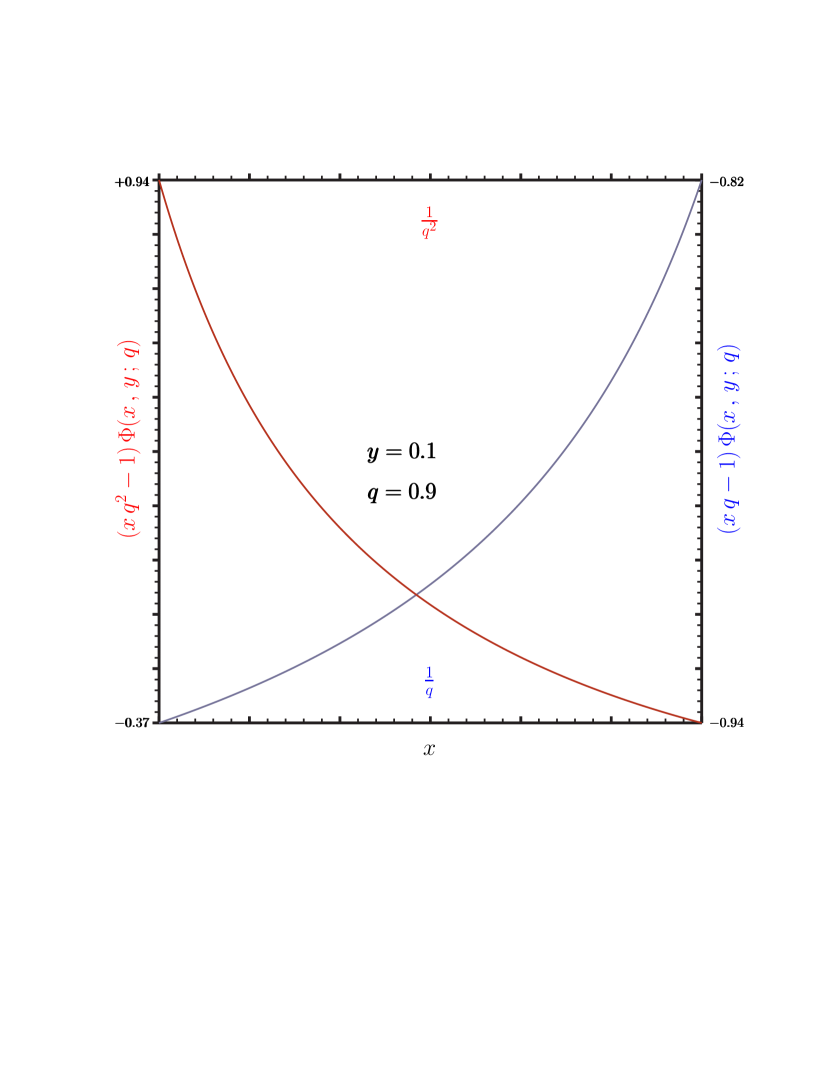
Figure 1: Behavior of $\Phi\left(x\,,\,y\,;\,q\right)$, defined in Eq.(14), around the poles at $x=1/q$ (blue curve) and $x=1/q^{2}$ (red curve).

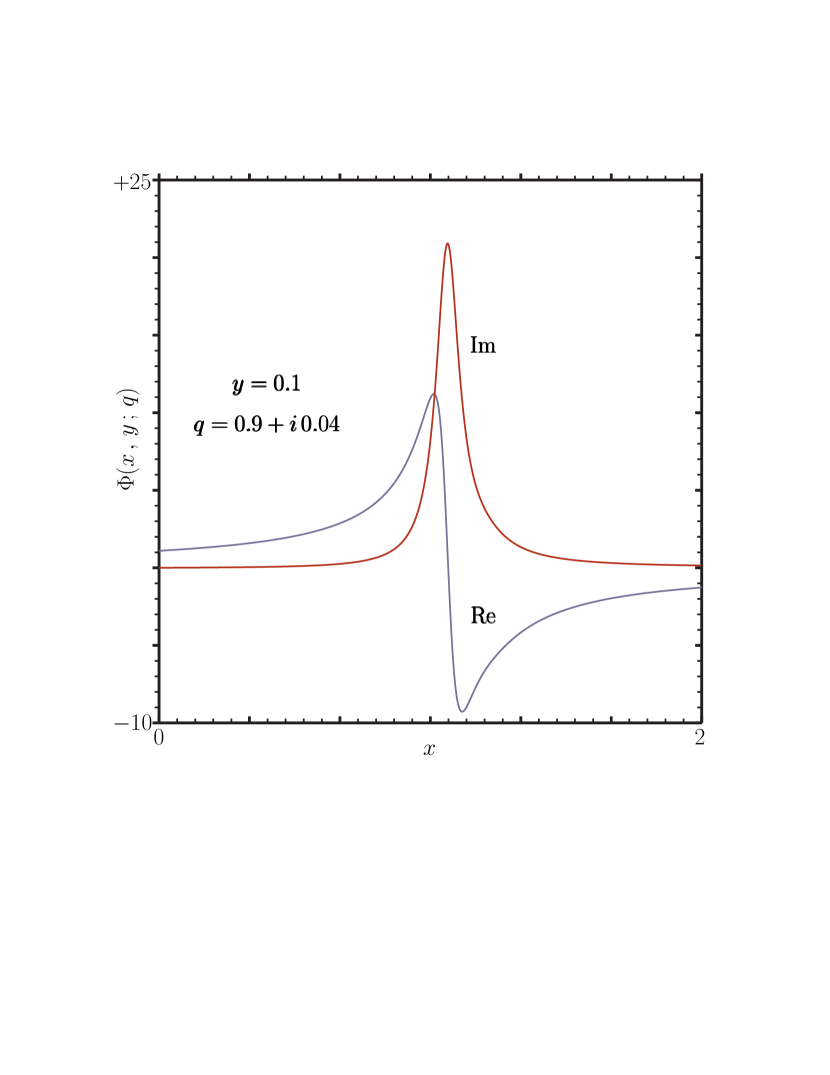
Figure 2: Behavior of $\Phi\left(x\,,\,y\,;\,q\right)$, defined in Eq.(14), as a function of $x$ for $y=0.1$ and $q=0.9+i\,0.04$.

Figure 3: The function $\mathrm{eli}_{1\,;\,0}(x\,,\,y\,;\,q)$, Eq.(72), for different values of $y$ and $q$ and $1/q_{{\mathrm{r}}}<x<1/q^{2}_{{\mathrm{r}}}$, $q_{{\mathrm{r}}}=\mathop{\mathrm{Re}}\nolimits\,q$.