Measuring neutron star tidal deformability with Advanced LIGO: a Bayesian analysis of neutron star - black hole binary observations
Abstract
The pioneering discovery of gravitational waves (GW) by Advanced LIGO has ushered us into an era of observational GW astrophysics. Compact binaries remain the primary target sources for GW observation, of which neutron star - black hole (NSBH) binaries form an important subset. GWs from NSBH sources carry signatures of (a) the tidal distortion of the neutron star by its companion black hole during inspiral, and (b) its potential tidal disruption near merger. In this paper, we present a Bayesian study of the measurability of neutron star tidal deformability using observation(s) of inspiral-merger GW signals from disruptive NSBH coalescences, taking into account the crucial effect of black hole spins. First, we find that if non-tidal templates are used to estimate source parameters for an NSBH signal, the bias introduced in the estimation of non-tidal physical parameters will only be significant for loud signals with signal-to-noise ratios greater than . For similarly loud signals, we also find that we can begin to put interesting constraints on (factor of ) with individual observations. Next, we study how a population of realistic NSBH detections will improve our measurement of neutron star tidal deformability. For an astrophysically likely population of disruptive NSBH coalescences, we find that events are sufficient to constrain within , depending on the neutron star equation of state. For these calculations we assume that LIGO will detect black holes with masses within the astrophysical mass-gap. In case the mass-gap remains preserved in NSBHs detected by LIGO, we estimate that approximately additional detections will furnish comparable measurement accuracy. In both cases, we find that it is the loudest events that provide most of the tidal information, and not the combination of tens of low-SNR events, thereby facilitating targeted numerical-GR follow-ups of NSBHs. We find these results encouraging, and recommend that an effort to measure be planned for upcoming NSBH observations with the LIGO-Virgo instruments.
I Introduction
The Advanced LIGO (aLIGO) observatories completed their first observing run “O1” early-2016, operating at a factor of higher gravitational-wave (GW) strain sensitivity than their first-generation counterparts Shoemaker (2010). During O1, they made the first direct observation of gravitational waves Abbott et al. (2016a). Emitted by a pair of coalescing black holes, these waves heralded an era of observational GW astrophysics as they traveled through Earth. Towards the end of this decade, we expect aLIGO to reach its design sensitivity. In addition to the US-based efforts, we also expect the French-Italian detector Advanced Virgo The Virgo Collaboration (2009); Acernese et al. (2015), Japanese detctor KAGRA Aso et al. (2013); Somiya (2012), and LIGO-India Unnikrishnan (2013) to begin observing at comparable sensitivities within a few years. With a global network of sensitive GW observatories, we can expect GW astronomy to face significant developments over the coming years.
Coalescing compact binaries of stellar-mass black holes (BH) and/or neutron stars (NS) are the primary targets for the second generation GW detectors Timmes et al. (1996); Fryer (1999); Woosley et al. (2002); Belczynski et al. (2010a, b); Dominik et al. (2015); Belczynski et al. (2007); Fryer et al. (2012); Wex and Kopeikin (1999); Narayan et al. (1991); Mandel et al. (2015); Abbott et al. (2016b). A binary system of black holes was recently observed by aLIGO Abbott et al. (2016a). Previously, stellar-mass black holes had only been observed by inference in mixed binaries with stellar companion (through electromagnetic observations of the companion) Psaltis et al. (2010); Remillard and McClintock (2006); Fragos et al. (2010). Neutron stars, on the other hand, have had numerous sightings. Thousands of electromagnetically emitting neutron stars, or pulsars, have been documented Manchester et al. (2005), in varied situations: as radio pulsars Lattimer (2012); Manchester et al. (2005), in binary systems with a stellar companion Margon et al. (1971); Bond et al. (2002); Lattimer (2012); Manchester et al. (2005), and in binary neutron stars (BNS) Hulse and Taylor (1975); Taylor and Weisberg (1982); Weisberg et al. (2010); Lattimer (2012); Manchester et al. (2005). Mixed binaries of black holes and neutron stars, is an astrophysically interesting class of systems Wex and Kopeikin (1999); Narayan et al. (1991); Janka et al. (1999); Fryer et al. (2015), that has not yet been detected. We expect to observe mixed binaries per year with aLIGO Abadie et al. (2010).
NSBH binaries are of interest for multiple reasons. For instance, they have been long associated with (as possible progenitors of) short Gamma-ray Bursts (SGRBs) Eichler et al. (1989); Narayan et al. (1992); Mochkovitch et al. (1993); Barthelmy et al. (2005); Fox et al. (2005); Gehrels et al. (2005); Shibata et al. (2006); Paschalidis et al. (2015); Tanvir et al. (2013). Depending on their equation of state (EoS), NSs can get disrupted by the tidal field of their companion BHs. Once disrupted, most of the NS material falls into the hole over an ms time-scale, with the rest partly getting ejected as unbound material and partly forming an accretion disk around the BH. This short lived () disk-BH system is hypothesized to drive SGRBs through the production of relativistic jets Foucart et al. (2015); Lovelace et al. (2013); Deaton et al. (2013); Foucart (2012); Shibata et al. (2006); Paschalidis et al. (2015). However, whether or not such a system forms depends also on the nature of the BH. Massive BHs (with ), as well as BHs with large retrograde spins, tend to swallow the NS whole without forming a disk Foucart et al. (2013a). On the other hand, low-mass BHs with 111 The upper limit on BH mass that allows for NS disruption may very well be higher, depending strongly on the magnitude of BH spin Foucart et al. (2014)., can disrupt their companion NSs much before merger, forming long-sustained disks that are required to sustain SGRBs Shibata and Taniguchi (2008); Ferrari et al. (2010); Lovelace et al. (2013); Foucart et al. (2014); Kawaguchi et al. (2015). A coincident detection of both GWs and gamma-rays from an NSBH merger, will provide us with a unique opportunity to confirm this hypothesized link between NSBH mergers and GRBs Abbott et al. (2016c).
Another question that compact object mergers can help answer is ‘what is the nature of matter at nuclear densities supported by NSs’? A large fraction of past work aimed at measuring NS matter effects from GW signals has consisted of inquiries about BNSs Lee and Kluzniak (1999a, b); Lee (2000); Oechslin et al. (2007); Read et al. (2009); Markakis et al. (2010, 2009); Stergioulas et al. (2011); East et al. (2012); Lackey and Wade (2015); Wade et al. (2014); Bauswein et al. (2014). In this paper, we will instead focus on NSBHs. During the course of early inspiral, the tidal field of the BH produces a deformation in its companion NS. The quadrupolar moment of the star associated with this deformation also depends on its material properties, through an EoS-dependent tidal deformability parameter . This induced quadrupolar moment changes over the orbital time-scale, resulting in the emission of GWs in coherence with the orbital waves. These waves draw more energy from the orbit and increase the inspiral rate (as compared to an equivalent BBH) Flanagan and Hinderer (2008). Closer to merger, the strong tidal field of the BH can disrupt the NS. The quadrupolar moment of the disrupted binary system falls monotonically over a millisecond time-scale Kyutoku et al. (2010); Lackey et al. (2014); Lovelace et al. (2013); Foucart et al. (2015); Pannarale et al. (2015a), resulting in the damping of GW amplitude. This penultimate stage also depends strongly on the internal structure and energy transport mechanism of the NS, and carries the strongest tidal signature in the GW spectrum Foucart et al. (2014); Deaton et al. (2013).
Gravitational waves emitted by coalescing NSBH binaries carry subtle hints of the NS EoS from inspiral through to merger. During early inspiral, the tidal dephasing is relatively weak and has a frequency dependence equivalent to a Post-Newtonian (PN) order effect Vines et al. (2011). Closer to merger, a disruptive fate of the NS can result in a strong suppression of GW emission above a cut-off frequency Pannarale et al. (2015a). Some past studies of tidal measurements with NSBH binaries have used PN inspiral-only waveforms Maselli et al. (2013). In doing so, however, they ignore (i) the merger signal which could contain significant information for NSBHs, and (ii) the errors due to unknown vaccum terms in PN waveforms, which could dominate over the tidal terms themselves Barkett et al. (2016); Yagi and Yunes (2014). Some other studies that account for merger effects via the use of complete numerical simulations Foucart et al. (2013a), are limited in the binary parameter space they sample. Others, that do the same through the use of phenomenological waveform models Lackey et al. (2012, 2014) use the Fisher matrix to estimate measurement errors. Fisher matrix estimates may become unreliable at realistic signal-to-noise ratios (SNR) Vallisneri (2008), such as those as we might expect in the upcoming observing runs of GW detectors Abadie et al. (2010), and we improve such studies with a fully Bayesian treatment of the problem here.
In this paper we study the measurability of neutron star’s tidal deformability from realistic binaries of low-mass BHs and NSs by aLIGO. We also probe how tidal effects affect the estimation of other binary parameters for the same class of systems. This study improves upon previous work in the following ways. First, we include tidal effects during inspiral and merger in a consistent way, by using the waveform model of Lackey et al. Lackey et al. (2014) (abbreviated henceforth to “LEA”). Second, we include the effect of black hole spin on tidal GW signals, in addition to the effect of BH mass, tidal deformability of the NS, and the SNR. Third, we perform a complete Bayesian analysis, instead of using the Fisher matrix approximation. And fourth, we explore how our measurement errors decrease as we gain information from multiple (realistic) events.
We now outline the main questions and results discussed in this paper. First, we probe the effect of ignoring tidal effects in the recovery of non-tidal binary parameters, such as component masses and spins. This is the case for current and planned aLIGO efforts. To do so, we first use the enhanced-LEA (or “LEA+”, see Sec. II.1) model to generate a set of realistic signals; and then use non-tidal (BBH) waveform filters to estimate the underlying binary masses and spins with a Markov-chain Monte Carlo. Here and throughout, we use the zero-detuning high-power design sensitivity curve Shoemaker (2010) to characterize the expected detector noise. We find that, for individual events, ignoring tidal effects will affect mass and spin-estimation only marginally; only for very loud signals (SNRs ) will the systematic biases be large enough to exceed the underlying statistical uncertainty. Furthermore, detection searches can ignore tidal effects without loss of sensitivity.
Second, we study the ability of aLIGO to constrain neutron star tidal deformability with a single observation of an NSBH merger. For this, we use the same setup for signal waveforms as before, but replace the filter template model with one that includes tidal effects from inspiral through to merger (i.e. LEA+) Lackey et al. (2014). For most binaries with BH masses outside of the mass-gap Bailyn et al. (1998); Kalogera and Baym (1996); Kreidberg et al. (2012); Littenberg et al. (2015) and/or realistic signal-to-noise ratios (SNR), we find it difficult to put better than a factor of bound on with a single observation. As we can see from Fig. 6, it is only at SNRs (under otherwise favorable circumstances, such as a stiff equation of state) that we are able to bring this down to a bound on . For signals louder than , we can constrain to a much more meaningful degree (within of its true value). While this is discouraging at first, we turn to ask: what if we combine information from a population of low-SNR observations?
The EoS of matter at nuclear densities is believed to be universal among all neutron stars. The Tolman-Oppenheimer-Volkoff equation Tolman (1939); Oppenheimer and Volkoff (1939); Tolman (1934) would then predict that NS properties satisfy a universal relationship between and . As the final part of this paper, we combine information from multiple observations of realistic NSBH systems and perform a fully-Bayesian analysis of how our estimation of changes as we accumulate detections. This is similar to an earlier study Del Pozzo et al. (2013) aimed at binary neutron stars. We restrict ourselves to a population of NSs with masses clustered very tightly around (with a negligible variance), and negligible spins. We sample different nuclear EoSs by sampling entire populations fixing different values for the NS tidal deformability. For all populations, we take source locations to be uniformly distributed in spatial volume, and source orientations to be uniform on the sphere. To summarize, we find the following: (a) Our median estimate for starts out prior dominated, but converges to within of the true value within detections. (b) Measurement uncertainties for , on the other hand, depend on itself. We find that for hard equations of state (with ), observations are sufficient to constrain within . For softer equations of state, the same level of certainty would require substantially more () observations. (c) Further, if the astrophysical “mass-gap” Bailyn et al. (1998); Kalogera and Baym (1996); Kreidberg et al. (2012); Littenberg et al. (2015) is real, we find that additional observations would be required to attain the same measurement accuracy as above. (d) Putting tighter constraints on the of a population would require NSBH observations, in any scenario. And, (e) it is the loudest events that will furnish the bulk of tidal information, and not the combination of a large number of low-SNR events. All of the above is possible within a few years of design aLIGO operation Abadie et al. (2010).
In this paper, we restrict our parameter space to span mass-ratios , dimensionless BH spin (aligned with orbit) , and dimensionless NS tidal deformability . These ranges are governed by the calibration of the LEA+ model which we use as filters. Most of the disruptive NSBH simulations that LEA+ has been calibrated to involve NSs, and it is unclear how reliable the model is for different NS masses Lackey et al. (2014); Pannarale et al. (2015b). This motivates us to conservatively fix NS masses to in our simulated signals (not templates). But, since the domain of calibration of LEA+ excludes NS spin completely, we fix in both signals as well as filter templates. We expect the effect of ignoring NS mass and spin variations in our NSBH populations to be less severe than for BNSs Agathos et al. (2015), considering the higher mass-ratios of NSBHs. The accuracy of our quantitative results depends on the reliability of LEA+, which is the only model of its kind in current literature. A more recent work Pannarale et al. (2015b) improves upon the amplitude description of LEA+, but needs to be augmented with a compatible phase model. Overall, we expect our broad conclusions here to hold despite modeling inaccuracies (with errors not exceeding Pannarale et al. (2015b)). Finally, our results apply to LIGO instruments at design sensitivity, which they are projected to attain by Shoemaker (2010); Abbott et al. (2016c).
The remainder of the paper is organized as follows. Sec. II discusses data analysis techniques and resources used in this paper, such as the waveform model, and parameter estimation algorithm. Sec. III discusses the consequences of ignoring tidal effects in parameter estimation waveform models. Sec. IV discusses the measurability for the leading order tidal parameter at plausible SNR values. Sec. V discusses the improvement in our measurement of with successive (multiple) observations of NSBH mergers. Finally, in Sec. VI we summarize our results and discuss future prospects with Advanced LIGO.
II Techniques

II.1 Waveform Models
Lackey et al. (LEA) Lackey et al. (2014) developed a complete inspiral-merger waveform model for disrupting NSBHs. Theirs is a frequency-domain phenomenological model that includes the effect of BH and NS masses and spins and NS tidal deformability . It was calibrated to a suite of numerical relativity (NR) simulations of NSs inspiraling into spinning BHs, with NS masses ranging between , mass-ratios , and BH spins . They also sample a total of two-parameter nuclear EoSs to cover the spectrum of NS deformability. The GW strain per the LEA model can be written as
| (1) |
with NS spin identically. Here, is an underlying BBH waveform model. In the original LEA model, this was taken to be the SEOBNRv1 model Taracchini et al. (2012) of the Effective-one-body (EOB) family Buonanno and Damour (1999). The factor adjusts the amplitude of the BBH model to match that of an NSBH merger of otherwise identical parameters, with NS-matter effects parametrized by . During early inspiral this term is set to unity, but is a sensitive function of close to merger. The term with corrects the waveform phasing. During inspiral, is set to the PN tidal phasing corrections, at the leading and next-to-leading orders Vines et al. (2011); close to merger, additional phenomenological terms are needed. Both and are calibrated to all available NR simulations.
In this paper we use LEA for our signal and template modeling, but switch the underlying BBH model to SEOBNRv2 (and refer to it as enhanced-LEA or “LEA+”) Taracchini et al. (2014). We using the reduced-order frequency-domain version of SEOBNRv2, which has the additional benefit of reducing computational cost Pürrer (2015). We expect this enhancement from LEALEA+ to make our conclusions more robust because: (a) the SEOBNRv2 model is more accurate Kumar et al. (2015, 2016), and (b) the differences between the two EOB models are caused by the inaccuracies of SEOBNRv1 during the inspiral phase, many orbits before merger Kumar et al. (2015). Since LEA only augments inspiral phasing with PN tidal terms, our change in the underlying BBH model does not change LEA’s construction, and increases the overall model accuracy during inspiral. Finally, we note that we approximate the full GW signal with its dominant modes, that are modeled by LEA+. For use in future LIGO science efforts, we have implemented the LEA+ model in the LIGO Algorithms Library Collaboration .
II.2 Bayesian methods
The process of measuring systematic and statistical measurement errors involves simulating many artificial GW signals, and inferring source binary parameters from them using Bayesian statistics. We start with generating a signal waveform, using the model LEA+, and injecting it in zero noise to obtain a stretch of data . Source intrinsic parameters are reconstructed from this injected signal. Extrinsic parameters representing the time of and phase at the arrival of signal are marginalized over numerically and analytically (respectively), while source location and orientation parameters such as its luminosity distance, sky location, inclination and polarization angles are absorbed into a normalization, as describe later, and subsequently maximized over. This is justified because in this paper we consider the single-detector case. Using Bayes’ theorem, the joint inferred probability distribution of can be evaluated as
| (2) |
Here, is the a priori probability of binary parameters taking particular values, given - which denotes all our collective knowledge, except for expectations on binary parameters that enter our calculations explicitly. Throughout this paper, we impose priors that are uniform in individual component masses, BH spin, and the tidal deformability of the NS. In addition, we restrict mass-ratios to , as LEA+ is not calibrated for . is the likelihood of obtaining the given stretch of data if we assume that a signal parameterized by is buried in it, and is given by
| (3) |
where is a filter template with parameters , is a suitably defined detector-noise weighted inner-product222The inner product is defined as (4) where is the Fourier transform of the finite time series , and is the one-sided amplitude spectrum of detector noise. In this work, we use the zero-detuning high-power design sensitivity curve Shoemaker (2010) for Advanced LIGO, with Hz as the lower frequency cutoff., and is the normalization constant that absorbs source distance, orientation and sky location parameters. As in Ref. Pürrer et al. (2015) we use a likelihood that is maximized over the template norm, allowing us to ignore the extrinsic parameters that only enter in the template norm through . As a result, we only need to sample over (or in the case of non-tidal templates). The denominator in Eq. 2 is the a priori probability of finding the particular signal in and we assume that each injected signal is as likely as any other. From the joint probability distribution so constructed, extracting the measured probability distribution for a single parameter (say ) involves integrating
| (5) |
where is the set of remaining parameters, i.e. .
We use the ensemble sampler Markov-chain Monte-Carlo algorithm implemented in the emcee package Foreman-Mackey et al. (2013), to sample the probability distribution . We run 100 independent chains, each of which is allowed to collect 100, 000 samples and combine samples from chains that have a Gelman-Rubin statistic Gelman and Rubin (1992) close to unity. This procedure yields about 10,000 independent samples. One simplification we make to mitigate computational cost is to set the frequency sampling interval to Hz, which we find to be sufficient for robust likelihoods calculations in zero noise Pürrer et al. (2015). We integrate Eq. 5 to obtain marginalized probability distributions for the NS tidal deformability parameter: . We will quote the median value of this distribution as our measured value for , and the credible intervals associated with the distribution as the statistical error-bars.
III How is PE affected if we ignore NS matter effects?
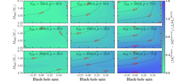
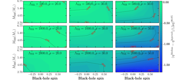
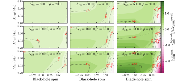

Past (and future) efforts with Advanced LIGO have used (or plan to use) BBH waveform templates to search for and characterize NSBH sources. In doing so, they ignore the signature of NS tidal effects on the emitted GWs. In this section we present a fully Bayesian analysis of the effect of this simplification on the recovery of non-tidal parameters from NSBH signals.
We inject LEA+ NSBH signals into zero noise, and run an MCMC sampler on them using equivalent BBH templates (same model, tidal terms ). We fix and , and explore a range of NS equations of state via the single tidal deformability parameter . Our injections also span a rectangular grid in the BH parameter space, with vertices at , i.e. , and BH spins . Finally, we sample all other source-related parameters, that determine the signal strength but not character333For aligned-spin signals and aligned-spin templates both, we only consider the contribution of the dominant waveform multipoles. This approximation has the additional benefit of combining the dependence of the waveforms on inclination, polarization and sky location angles, as well as on distance, into the luminosity or effective distance. This quantity only appears as an overall scaling factor, and therefore only affects signal strength Sathyaprakash and Schutz (2009). , by sampling the SNR . Our choice of injection parameters here is motivated by two factors: (i) previous studies of the signatures of NS tidal effects on gravitational waves Foucart et al. (2012, 2013a, 2014) (which suggest that necessary conditions for the observation of tidal effects with aLIGO include high SNRs and a low-mass spinning companion BH); and (ii) technical constraints of our chosen LEA+ model Lackey et al. (2014). At design sensitivity, if we expect NSBH detections a year Abadie et al. (2010), we can expect to see disruptive444We assume here that BH mass values are uniformly likely from to Abbott et al. (2016a), but NSs are disrupted in NSBH mergers only if and Foucart et al. (2014, 2013a). NSBH mergers a year, of which we will have observations with , and a year with . Therefore, our injection parameters span a physically interesting subset of NSBH binaries, that is also likely observable in the near future. For our Bayesian priors, we choose uniform distributions for both component masses and black hole spin: ; ; and .
The effect of ignoring tidal corrections in templates will manifest as a systematic shift of recovered median parameter values away from what they would be if we had used tidal templates with identical priors. In zero noise, we expect the probability distributions recovered using tidal templates to be multi-dimensional Gaussians with the maximum likelihood parameter values approaching their true values. If the priors are not restrictive, we expect the recovered median to also converge to the true value. However, the LEA model imposes significantly more restrictive priors (both mass-ratio and spin) than SEOBNRv2 Taracchini et al. (2014); Lackey et al. (2014), which shifts the median value of parameters recovered using our tidal templates away from their true value. If we use LEA+ priors for our non-tidal templates, it would add a caveat to our original question ’can we estimate non-tidal NSBH parameters with equivalent BBH templates’. Instead, we approximate the median tidally recovered parameters by their true injected values, as one would expect to recover with an ideal model for tidally disruptive NSBH mergers. With this caveat, we estimate systematic measurement bias/errors as the differences between median and injected parameter values. As an illustration, in Fig. 1 we show the recovered probability distributions for binary mass ratio for three NSBH injections, with (left), (middle), and (right), and other parameters held fixed (, , , and ). In each panel, both the true and median values of are marked, and we use the shift between the red and green vertical lines as our estimate of systematic measurement errors. Darker shading in all panels marks credible intervals, whose width we use as a direct measure of our statistical measurement uncertainty/error555We generalize the notation to mean the credible interval width for any measured source parameter .. For the illustrated binary, we see clearly that even when the signal is moderately loud, with , statistical errors dominate over systematics for . As we turn up the SNR further, the two error sources become comparable at , and systematic errors dominate finally when .
Credible intervals showing the precision with which can be measured, are presented in Appendix A. We remind ourselves that this precision is only meaningful so long as the measurement is accurate to begin with. Therefore, we define as the ratio between systematic and statistical errors associated with the measurement of parameter ,
| (6) |
in order to compare the relative magnitude of both. Only when can we ignore tidal effects in our templates without hampering the measurement of non-tidal parameters from NSBH signals. When approaches a few tens of percent of unity, we can begin to favor tidal templates for NSBH studies.
We start with calculating as a function of various source parameters and show it in Fig. 2. is the leading order mass combination that affects the GW strain emitted by compact binaries as they spiral in, and is therefore determined the most precisely. We notice immediately that for the systematics are well under control and we can obtain reliable chirp mass estimates for NSBH signals using BBH templates. For louder and less likely SNRs (), we find that can become comparable to unity, but only if the BH has prograde spin , and the true NS tidal deformability is large enough, s.t. . We therefore conclude that only for very loud signals, with , will the inclusion of tidal terms in template models improve estimation. For lower SNRs, inclusion of new physical content in templates will instead get washed out by detector noise. In addition, we also note that always, i.e. is always being over-estimated. This is to be expected since the tidal deformation of the NS drains energy faster from the orbit during inspiral (as compared to the BBH case), and its disruption close to merger reduces GW signal power at high frequencies. Both of these effects make the resulting signal resemble a BBH signal of higher chirp (or total) mass, although we expect the latter effect to be dominant Pannarale et al. (2011).
Next, in Fig. 3, we show the ratio of measurement errors for the symmetric mass-ratio. Going through the figure from left to right, we find that for realistic SNRs () the systematics remain below statistical errors for measurement. The worst case is of the most deformable NSs (), but even for them systematics in are smaller than the statistical measurement errors. Moving to louder signals with , we find that for binaries of fairly deformable NSs () and low-mass BHs () that have prograde spins (), our measurement of mass-ratio can be seriously compromised by ignoring tidal physics in template models. This pattern is continued at even higher SNRs, as we can see from Fig. 3. We therefore conclude that, even if under moderate restrictions on BH and NS parameters, is loud enough to motivate the use of tidal templates in aLIGO data analyses. In addition, we also notice that, unlike for , the median value of is always lower than its true value, which is what we expect if we want BBH templates to fit NSBHs that disrupt and merge at lower frequencies.
Moving on from mass to spin parameters, we now consider the measurement of BH spin angular momentum . The ratio of systematic and statistical errors for are shown in Fig. 4. The presentation of information in this figure is identical to that of Fig. 2 and 3. A diverging colormap is used so that both extremes of the colorbar range point to large systematic biases, while its zero (or small) value lies in the middle. For the lowest SNR considered (), bias is about smaller than its statistical measurement uncertainty, and is therefore mostly negligible. Both do become somewhat comparable, but only when we have the most deformable NSs in orbit around low-mass BHs. At higher SNRs , we find that the systematics in measurement can dominate completely, especially for binaries containing mass-gap violating BHs and/or deformable NSs with . From Fig. 4 we additionally note that when the source spin magnitudes approach the highest allowed, i.e. at both extremes of the -axes, . This is to be expected because the median of the recovered posterior distributions for can only get pushed inwards from the boundaries.
Summarizing these results, we find that irrespective of system parameters, below a signal-to-noise ratio of , our measurements of mass and spin parameters of astrophysical NSBH binaries will remain limited by the intrinsic uncertainty due to instrument noise, and do not depend on whether we include tidal effects in template models. However, when the signal-to-noise ratio exceeds the systematic bias in binary mass and spin measurements become comparable to and can exceed the uncertainty due to noise. Of the different non-tidal parameters considered, we find that the measurement of degrades worst (in a relative-error sense) due to the use of BBH templates in deciphering an NSBH signal. Of all the sub-categories, we find that tidal templates could especially help with the parameter estimation of astrophysical mass-gap violating NSBH binaries,
IV What do we gain by using templates that include NS matter effects?
In the previous section, we showed that the effects of the tidal deformation of NSs by their companion BHs become discernible in the GW spectrum under certain favorable conditions, including (a) BH mass is sufficiently small, (b) BH spin is positive aligned, i.e. , (c) the NS is not very compact, with , and (d) the source location and orientation are such that its GW SNR . Both condition (a) and (b) enhance the tidal distortion of the star and increase the number of orbits the system goes through at small separation, where the differences between NSBH and BBH signals are maximal. Conditions (a)-(c) also reduce the onset frequency of the disruption of the NS, allowing for it to happen earlier in the orbit. We expect that these conditions are also the ones which should maximize the likelihood of measuring tidal effects in NSBH signals. Here, we turn the question around to ask: under similarly favorable circumstances, can we gain insights about the internal structure of neutron stars from GW observations?
In this section, we calculate the accuracy with which we measure from single GW observations. We sample the same set of disruptive NSBH mergers as in the previous section, i.e. those with , , and ; fixing the NS mass and . For each unique combination of these parameters, we inject LEA+ signals into zero noise and perform a fully Bayesian parameter estimation analysis of each with LEA+ templates. Our priors on component masses and spins remain as in the previous section, with mass-ratio additionally restricted to , and sampled uniformly from . As an illustration of individual injections, we show the recovered probability distribution for for three specific configurations in Fig. 5. We fix , with , and vary over between the three panels. The SNR is fixed at . The darker shaded regions mark the credible interval on . We note that is estimated to within of its true value at this SNR. Another interesting thing to note is that while slowly grows with , the fractional uncertainty
| (7) |
decreases instead. Further illustrations, showing the correlation between tidal and non-tidal parameters, are presented in Appendix B. We will continue here to focus on the measurement of itself.
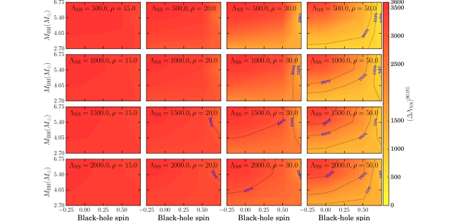
In Fig. 6 we show the main results of this section. In each panel, as a function of black hole mass and spin, we show the measured credible interval widths . These correspond to the full width of the dark shaded regions in the illustrative Fig. 5. The effect of increasing signal strength can be seen as we go from left to right in each row. The effect of the NS tidal deformability parameter on its own measurability can be seen by comparing panels within each column, with the NS becoming more deformable from top to bottom. A uniform pattern emerges in the left-most column, which corresponds to . We find that at this signal strength, our measurement of is dominated by the width of our prior on it. The credible intervals span the entire allowed range for , making a reasonable estimation of at difficult. Increasing the signal strength to gives marginally better results, bringing down the statistical uncertainties to within of the true value 666The symmetric error-bars of correspond to .. It is not until we reach an SNR as high as , can we put meaningful (i.e. ) constraints on . For e.g., with a single observation of a binary with and 777For an optimally oriented source with , an SNR of corresponds to a luminosity distance of Mpc., we would be able to estimate to within of its true value (which is equivalent to measuring the ratio of NS radius to mass with an uncertainty of about ). These results agree well with Sec. III, and are consistent with Fisher matrix estimates at high SNRs Lackey et al. (2014).
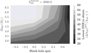
Amongst other source parameters, BH mass and spin play a dominant role. A smaller BH with a larger spin always allows for a more precise measurement on . We can see this in the bottom right corner of each panel in Fig. 6, which corresponds to low-mass BHs with large spins, and is simultaneously the region of smallest measurement errors on . The actual deformability of the NS also plays an important role on its own measurability. For e.g., when , it is fairly difficult to meaningfully constrain without requiring the source to be close (Mpc) with a GW SNR . Quantifying this further, in Fig. 7 we show the minimum signal strength required to attain a certain level of credibility in our measurement, as a function of BH properties. The NS is allowed the most favorable (hardest) EoS considered, with . We first note that, even with the most favorable BH and NS properties, achieving a measurement certainty on will require a GW SNR . If we additionally restrict BH masses to lie outside of the so-called astrophysical mass-gap Bailyn et al. (1998); Kalogera and Baym (1996); Kreidberg et al. (2012); Littenberg et al. (2015), we will simultaneously need to restrict BH spins to to obtain the same measurement credibility at the same source location.
It is interesting to note that the parameter ranges most favorable to the measurability of are also those which produce relatively more massive post-merger disks Foucart (2012). That is, the subset of NSBHs that potentially produce SGRBs (using a sufficiently-large disk mass as an indicator) would be the same subset most favorable for measurement of tidal effects. Therefore the rate of SGRBs in the local universe (allowing for the fraction that are produced by NSBHs versus BNSs) would be an indicator of the rate of events most favorable for nuclear equation of state measurements.
In summary, with a single moderately loud () GW signal from a disruptive BHNS coalescence, we can constrain the NS compactness parameter within of its true value. To measure better with one observation, we will need a more fine-tuned source, with and high BH spins, or . Finally, we note that these results are conservative, and BHs with spins will prove to be even more favorable laboratories for measurement. However, we are presently unable to explore this case in quantitative detail due to waveform model restrictions Lackey et al. (2014), which will also restrict our analyses of GW signals during the upcoming LIGO observing runs.
V Combining observations: looking forward with Advanced LIGO
In the previous section, we showed that single observations of NSBH coalescences at moderate SNRs have little information about the internal structure of neutron stars that will be accessible to Advanced LIGO at its design sensitivity. We expect all neutron stars to share the same equation of state, and hence the same . In addition, we know that the mass distribution of (most) NSs that have not been spun up to millisecond periods (which are the ones we focus on in this paper, by setting ) is narrowly peaked around Kiziltan et al. (2013). Therefore, information from multiple NSBH observations can be combined to improve our estimation of . We explore the same in this section within a fully Bayesian framework. We refer the reader to Ref. Mandel (2010); Lackey and Wade (2015); Wade et al. (2014) for similar analyses of BNS inspirals.
An intuitive understanding of the problem is gained by considering first multiple identical sources with realistic but different SNRs. Let us consider the case of a population of optimally oriented binaries 888An optimally oriented binary is one which is located directly overhead the detector, with the orbital angular momentum parallel to the line joining the detector to the source. Such a configuration maximizes the observed GW signal strength in the detector., distributed uniformly in spatial volume out to a maximum effective distance 999effective distance is a combination of distance to the source, its orientation, and its sky location angles; and has a one-to-one correspondence with SNR for non-precessing sources. This is so because for such sources, their location and orientation remain constant over the timescales within which they sweep through aLIGO’s sensitive frequency band.. . is set by the minimum SNR threshold at which a source is considered detectable 101010which we take as throughout.. Next, we divide this volume into concentric shells, with radii . If we have a measurement error for , associated with a source located at , the same error for the same source located within the th shell would be . Ref. Markakis et al. (2010) calculated that the combined error from independent measurements of in such a setting to be
| (8) | ||||
where is the number of sources within the th shell (s.t. ), and is the number density of sources in volume. The root-mean-square (RMS) averaged measurement error from sources is then Markakis et al. (2010)
| (9) |
given a fiducial pair . It is straightforward to deduce from Eq. 9 that measurement uncertainty scales as , and the uncertainty afforded by a single observation with a high SNR can be attained with realistic observations that have . E.g., to get to the level of certainty afforded by a single observation with , we would need realistic (low SNR) detections.
While we discussed Eq. 9 for a population of optimally oriented sources, it is valid for a more general population distributed uniformly in effective volume Markakis et al. (2010) (). However, it still only applies to sources with identical masses and spins, and we overcome this limitation by performing a fully Bayesian analysis next.
Astrophysical source population: Imagine that we have stretches of data, , each containing a single signal emitted by an NSBH binary. Each of these signals can be characterized by the non-tidal source parameters , and , where contains extrinsic parameters, such as source distance, inclination, and sky location angles. As before, let denote all of our collective prior knowledge; for instance, includes our assumption that all NSs in a single population have the same deformability parameter , and that its cumulative measurement is therefore possible. The probability distribution for , given unique and independent events, is
| (10) | |||||
| (11) | |||||
| (12) |
where Eq. 10 and Eq. 12 are application of Bayes’ theorem, while Eq. 11 comes from the mutual independence of all events. Assuming in addition that all events are equally likely: , we get
| (13) | |||||
where the prior probability is written for brevity. A priori, we assume that no particular value of is preferred over another within the range , i.e.
| (14) |
With a uniform prior, the first two factors in Eq. 13 can be absorbed into a normalization factor , simplifying it to
| (15) |
In the second set of terms in Eq. 15 (of the form ), each is the probability distribution for inferred a posteriori from the i-th observation by marginalizing
| (16) |
where is the inferred joint probability distribution of all source parameters for the -th event, as given by Eq. 2. We note that Fig. 5 illustrates for three individual events. By substituting Eq. 14-16 into Eq. 15, we calculate the probability distribution for as measured using independent events.
Our goal is to understand the improvement in our measurement of with the number of recorded events. To do so, we simulate a population 111111A population here is an ordered set of events, and an event itself is the set of parameters describing one astrophysical NSBH binary. of events, and quantify what we learn from each successive observation using Eq. 15. This allows us to quantify how rapidly our median estimate for converges to the true value, and how rapidly our credible intervals for the same shrink, with increasing . Finally, we generate and analyze an ensemble of populations in order to average over the stochastic process of population generation itself.
In order to generate each population, the first step is to fix the NS properties: (i) NS mass , (ii) NS spin and (iii) NS tidal deformability fixed value chosen from . Next, we generate events, by sampling BH mass (uniformly) from , BH spin (uniformly) from , orbital inclination from , and source location uniform in spatial volume121212with a minimum SNR . We restrict ourselves to positive aligned BH spins, since binaries with anti-aligned spins have very little information to add at realistic SNRs, as demonstrated in Fig. 6. This is to be taken into account when the number of observations is related to detector operation time. We repeat this process till we have an ordered set of events. Since we want to analyze not just a single realization of an astrophysical population, but an ensemble of them, we make an additional approximation to mitigate computational cost. Complete Bayesian parameter estimation is performed for a set of simulated signals whose parameters are the vertices of a regular hyper-cubic grid (henceforth “G”) in the space of , with each sampled at , , and . All events in each population draw are substituted by their respective nearest neighbours on the grid G. Our chosen signal parameter distribution is different from some other studies in literature, which often sample from more astrophysically motivated population distribution functions Mandel (2010). We chose one that is sufficiently agnostic in absence of actual known NSBHs, and pragmatic enough for generating population ensembles.
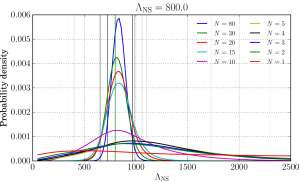
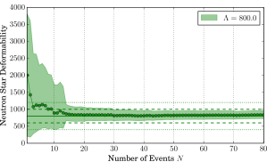
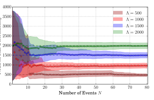
In Fig. 8 we show illustrative results for a single population with neutron star deformability . In the top panel, each curve shows the probability distributions for as inferred from events, with ranging from . We also mark the credible intervals associated with each of the probability distribution curves. The first few observations do not have enough information to bound much more than our prior from Eq. 14 does. In the bottom panel, we present information derived from the top panel. The line-circle curve shows the measured median value from observations. The pair of dashed (dotted) horizontal lines mark () error bars. At each , the range spanned by the filled region is the credible interval deduced from the same events. This figure somewhat quantifies the qualitative deductions we made from the left panel. We find that the median does track the true value quickly, reaching within its with observations. This is as one expects of injections in zero noise where random fluctuations are unable to shift the median away from the true value, so long as the measurement is not restricted by the prior. With the same information, our credible intervals also shrink to . In Fig. 9 we show further results from four independent populations for . As in the right panel of Fig. 8, the line-circle curves track the median , while the filled regions show the associated credible intervals. From the figure, we observe the following: (i) the shrinkage of credible interval widths with increasing happens in a similar manner for each , and (ii) it takes approximately events to distinguish definitively (with credibility) between deformable NSs with and compact NSs with , or equivalently to distinguish between hard, moderate and soft nuclear equations of state. This is comparable to what has been found for binary neutron stars Del Pozzo et al. (2013); Chatziioannou et al. (2015); Agathos et al. (2015).
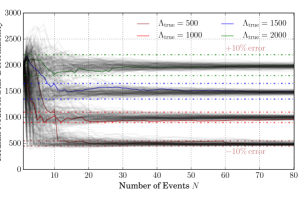
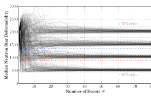
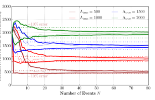
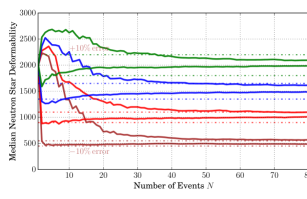
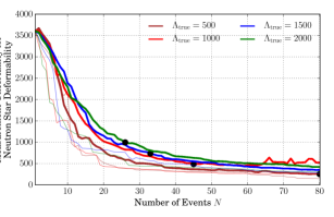
So far we have discussed individual realizations of NSBH populations. The underlying stochasticity of the population generation process makes it difficult to draw generalized inferences (from a single realization of an NSBH population) about the measurability of . In order to mitigate this, we discuss ensembles of population draws next. In Fig. 10 we show the median as a function of the number of observed events, for four population ensembles, with a hundred population draws in each ensemble. Lets focus on the top left panel first. In it, we show the median for all populations in four ensembles, with true from top to bottom. Populations highlighted in color are simply those that we discussed in Fig. 9. Dash-dotted horizontal lines demarcate error intervals around the true values. The panel just below it shows the range of that encloses the median for of the populations in each ensemble. In other words, this panel shows the range of within which the median value for of NSBH populations is expected to lie. From these panels, we observe that our median values will be within of the true value after detections of less deformable neutron stars (), or after as few as detections of more deformable neutron stars (). This is not surprising because we inject simulated signals in zero noise, which ensures that the median not be shifted away from the true value. That it takes events for the median to approach the true value is a manifestation of the fact that the measurement is limited by the prior on when we have fewer than events. The results discussed in Fig. 8, 9 and the left two panels of Fig. 10 apply to the parameter distribution spanned by the grid G. This distribution allows for as low as (i.e. ). Given that disruptive signatures are strongest for small , we now investigate an alternate paradigm in which no black hole masses fall within the mass gap suggested by astronomical observations Bailyn et al. (1998); Kalogera and Baym (1996); Kreidberg et al. (2012); Littenberg et al. (2015). We will henceforth denote our standard paradigm, which does not respect the mass-gap, as paradigm A; with paradigm B being this alternate scenario. Both right panels of the figure are identical to their corresponding left panels, but drawn under population paradigm B. Under this paradigm, we expectedly find that information accumulation is much slower. It would take detections with under this paradigm, for our median to converge within of its true value.
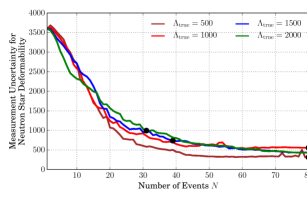
Finally, we investigate the statistical uncertainties associated with measurements. We use credible intervals as our measure of the same. First, we draw an ensemble of a hundred populations each for . For each population in each ensemble, we construct its credible interval . Next, we construct the interval that contains for of the populations in each ensemble; and similarly for . Finally, in the left panel of Fig. 11, we show the conservative width that contains the credible intervals for of all populations in each ensemble 131313Drawn under paradigm A (mass-gap not respected).. From top to bottom, the population decreases from , corresponding to decreasingly deformable NSs with softer equations of state. We observe the following: (i) for moderately-hard to hard equations of state with , we can constrain within using only events, and within (marked by black circles) with events; (ii) for softer equations of state with , we will achieve the same accuracy with and events, respectively; and (iii) for the first or so observations, our measurement spans the entire prior allowed range: , as shown by the plateauing of the credible intervals towards the left edge to of , i.e. . The right panel in Fig. 11 is identical to the left one, with the difference that populations are drawn under paradigm B, which does not allow for BH masses to fall within the mass-gap. We find that for NSs with , it would take events to constrain within and events to constrain it within . This is somewhat slower than paradigm A, as is to be expected since here we preclude the lowest mass-ratios, which correspond to signals with largest tidal signatures. For we find that we can constrain within with a similar number of events as for paradigm A, but will need more (, as compared to ) events to further constrain it to within of the true value. Under either paradigms, we find that measuring better than will require observations of disruptive NSBH mergers. These results demonstrate that our probed set of disruptive NSBH mergers is as informative of NS tidal properties as are BNS populations, if we assume a uniform mass distribution for NSs and zero NS spins, and possibly more if NS masses are not distributed uniformly Agathos et al. (2015). However, being a subset of all NSBH binaries, the accumulation of information from NSBH signals in general may be slower than from binary neutron stars, depending on the distribution of BH masses in coalescing NSBH binaries.
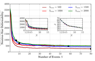
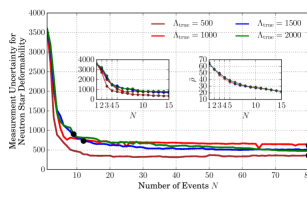
Do all events matter? In Ref. Lackey and Wade (2015) the authors demonstrate that the overwhelming majority of information about the NS equation of state comes from the loudest events in the case of binary neutron star detections, and not from the combined effect of a large number of low-SNR systems. The question naturally arises if the same is true for NSBH sources as well. Therefore, in Fig. 12 we re-evaluate the accumulation of information with each successive NSBH detection, sorting the events in each population by their SNR instead of simulated chronology. We find the same qualitative behavior as in the case of BNSs Lackey and Wade (2015). Whether or not there is an astrophysical mass gap, we find that the bulk of tidal information will be furnished by the loudest NSBH detections of aLIGO detectors. This result is especially encouraging to NR follow-up efforts for GW detections, as we now know that only a handful of loudest NSBH events (with SNRs ) are the ones that may merit full numerical-GR + magnetohydrodynamical follow-up simulations.
To summarize, in this section we study the improvement in our measurement of NS deformability parameter with an increasing number of events. We do so by simulating plausible populations of disrupting NSBH binaries (with ). We find that: (i) for more deformable neutron stars (harder equation of states), the median value of comes within of the true value with as few as events, while achieving the same accuracy for softer equations of state will take source detections; (ii) the statistical uncertainty associated with measurement shrinks to within with events, and to within with events, when source ; (iii) for softer equations of state, the same could take and events, respectively for the two uncertainty thresholds; and (iv) if BHs really do observe the astrophysical mass-gap, the information accumulation is somewhat slower than if they do not. We conclude that within observations, aLIGO would begin to place very interesting bounds on the NS deformability, which would allow us to rule out or rank different equations of state for neutron star matter. Within this population, we also find that it will be the loudest events that will furnish most of the tidal information. Our key findings are summarized in Fig. 10 - 12.
VI Discussion
The pioneering observation of gravitational waves by Advanced LIGO harbingers the dawn of an era of gravitational-wave astronomy where observations would finally drive scientific discovery Abbott et al. (2016d). As confirmed by the first observations Abbott et al. (2016d, e, b), stellar-mass compact binary mergers emit GWs right in the sensitive frequency band of the LIGO observatories, and are their primary targets. Neutron star black hole binaries form a physically distinct sub-class of compact binaries. We expect to detect the first of them in the upcoming observing runs Abbott et al. (2016f), and subsequently at a healthy rate of mergers a year when aLIGO detectors reach design sensitivity Abadie et al. (2010).
NSBH binaries are interesting for various reasons. Unlike BBHs, the presence of matter allows for richer phenomena to occur alongside the strong-field gravitational dynamics. The quadrupolar moment of the NS changes during the course of inspiral, which increases the inspiral rate of the binary and alters the form of the emitted gravitational waves. Close to merger, under restricted but plausible conditions, the neutron star is disrupted by the tidal field of its companion black hole and forms an accretion disk around it. This disruption reduces the quadrupolar moment of the system, and decreases the amplitude of the emitted GWs from the time of disruption through to the end of ringdown. Both of these phenomena are discernible in their gravitational-wave signatures alone. In addition, if the neutron star matter is magnetized, the magnetic winding above the remnant black hole poles can build up magnetic fields sufficiently to power short gamma-ray bursts (SGRB) Foucart et al. (2015); Lovelace et al. (2013); Deaton et al. (2013); Foucart (2012); Shibata et al. (2006); Paschalidis et al. (2015). Therefore a coincident observation of gravitational waves from an NSBH merger and a SGRB can potentially confirm the hypothesis that the former is a progenitor of the latter Eichler et al. (1989); Narayan et al. (1992); Mochkovitch et al. (1993); Barthelmy et al. (2005); Fox et al. (2005); Gehrels et al. (2005); Shibata et al. (2006); Tanvir et al. (2013); Paschalidis et al. (2015).
In this paper we study the observability of tidal signatures in the gravitational-wave spectrum of NSBH binaries. More specifically, we investigate three questions. First, what is the effect of not including tidal effects in templates while characterizing NSBH signals? Second, if we do include tidal effects, how well can we measure the tidal deformability of the NS (parameterized by ) from individual NSBH signals? And third, as we observe more and more signals, how does our knowledge of improve? In the following, we summarize our main findings.
First, we study the effects of not including tidal terms in our search templates while characterizing NSBH signals. We expect that the waveform template that best fits the signal would compensate for the reduced number of degrees of freedom in the template model by moving away from the true parameters of the binary. This should result in a systematic bias in the recovered values of non-tidal source parameters, such as its masses and spins. In order to quantify it, we inject tidal signals into zero noise, and perform a Bayesian parameter estimation analysis on them using templates without tidal terms. We use the LEA+ model (c.f. Sec. II.1) to produce tidal waveforms that incorporate the effect of NS distortion during inspiral, and of its disruption close to merger. Our injected signals sample the region of NSBH parameter space where NS disruption prior to binary merger is likely and can be modeled using LEA+. Their parameters are given by combinations of and . Other parameters, such as source location and orientation, that factor out of as amplitude scaling are co-sampled by varying .
At low to moderate SNRs (), we find that using BBH templates does not significantly hamper our estimation of non-tidal parameters for NSBH signals. In the worst case, when the BH mass is within the astrophysical mass-gap Bailyn et al. (1998); Kalogera and Baym (1996); Kreidberg et al. (2012); Littenberg et al. (2015) and its spin is positive aligned, the systematic biases in and measurements do become somewhat comparable to statistical errors (ratio ) under very restrictive conditions 141414requiring a companion BH with mass (i.e. in the astrophysical mass-gap), and the hardest NS EoS considered (with )., but never exceed them. At high SNRs (), systematic biases in become larger than the statistical uncertainties. For and the difference is more drastic with the systematics reaching up to the statistical errors. We therefore conclude that is loud enough to motivate the use of tidal templates for even the estimation of non-tidal parameters from NSBH signals. We also conclude that low-latency parameter estimation algorithms, designed to classify GW signals into electromagnetically active (NSBH and NSNS) and inactive (BBH) sources, can use BBH templates to trigger GRB alerts Abadie et al. (2012); Singer et al. (2014); Singer and Price (2016); Pankow et al. (2015); Abbott et al. (2016c, g) for NSBH signals with low to moderate SNRs (). This is so because the primary requirement of identifying NS-X binaries (X = {NS, BH}) can be achieved just as easily with BBH templates, on the basis of the smaller component’s mass151515The smaller component mass is unlikely to be significantly biased by missing tidal effects in filter templates below , as we show above.. We also speculate that NSBH detection searches are unlikely to be affected by the choice of ignoring tidal effects in matched-filtering templates, if these effects are too subtle to manifest in parameter estimation below .
Second, we turn the question around to ask: can we measure the tidal effects if our template models did account for them? Tidal effects in our waveform model are parameterized using a single deformability parameter . In order to quantify the measurability of , we inject the same tidal signals as before, and this time perform a Bayesian analysis on them using tidal templates. The results are detailed in Sec. IV. At low SNRs (), we find that the best we can do is to constrain within of its true value at credible level. This too only if the BH is spinning sufficiently rapidly, with , and the NS has . At moderate SNRs (), we can constrain a little better, i.e. within of its true value. This level of accuracy, however, again requires that BH spin and . Binaries with smaller BH spins and/or softer NS EoSs will furnish worse than errors for . This trend continues as we increase the SNR from . It is not before we reach an SNRs as high as that we can shrink errors substantially with a single observation (i.e. within of its true value). In summary, we find that with a single but moderately loud NSBH signal, Advanced LIGO can begin to put a factor of constraints on NS tidal deformability parameter. These constraints can subsequently be used to assess the likelihood of various candidate equations of state for nuclear matter, and possibly to narrow the range they span.
Third, knowing that single observations can furnish only so much information about the NS equation of state, we move on to investigate how well we do with multiple signals. In order to quantify how measurement improves with the number of observed events , we generate populations of NSBH signals and combine the information extracted from each event. The population generation procedure is as follows. The neutron star mass is held fixed at , its spin at , and its tidal deformability is fixed to each of . Black hole mass is sampled uniformly from the range , and spin from . As before, our parameter choice here is given by the intersection set of the mass range that allows for neutron star disruption and the range supported by LEA+ Foucart (2012); Foucart et al. (2013b); Lackey et al. (2014). In order to keep the computational cost reasonable, we make an additional approximation. For every population generated, we replace the parameters of each event by their nearest neighbor on the uniform grid G, which has vertices at: . This way, we only have to run full Bayesian parameter estimation analysis on this fixed set of signals. There are two sources of error that enter the deductions we make from a single population generated in the manner described above. First, since the injection parameters are pushed to their nearest neighbor on a grid, we find discrete jumps in errors as a function of . And second, an individual population is one particular realization of a stochastic process and could have excursions that may never be found in another population. To account for both of these limitations, we generate an ensemble of populations, and conservatively combine information from all of them161616See Sec. V for further details..
We probe two astrophysical paradigms, one that allows for BH masses to lie within the astrophysical mass-gap (paradigm A), and one that does not (paradigm B). For paradigm A, we find the following: (i) for the softer equations of state that result in less deformable neutron stars, detections bring the measured probability distribution for entirely within the prior, which ensures that the median tracks the true value to within . (ii) For NSBH populations with more deformable NSs (), the same is achievable within as few as (or at most) realistic observations. (iii) The statistical uncertainty associated with measurement can be restricted to be within using observations when ), and using observations for softer equations of state. All of the above is possible within a few years of design aLIGO operation Abadie et al. (2010), if astrophysical BHs are allowed masses (i.e. in the mass-gap). However, further restricting will require NSBH observations. For paradigm B, we find the information accumulation to be somewhat slower. While the quantitative inferences for populations with are not affected significantly, we find that populations require more events to attain the same measurement accuracy as under paradigm A. In either case, the accumulation of information from the general NSBH population will likely be slower than from BNS inspirals Mandel (2010); Lackey and Wade (2015); Wade et al. (2014); Agathos et al. (2015), depending on the mass distribution of stellar-mass black holes. Though, template models for the latter may be more uncertain due to missing point-particle PN terms at orders comparable to tidal terms Lackey and Wade (2015). We conclude that within as few as observations of disruptive NSBH mergers, aLIGO will begin to place interesting bounds on NS deformability. This, amongst other things, will allow us to rank different equations of state for neutron star matter from most to least likely, within a few years’ detector operation. We also find that, within this population, the loudest events (with SNRs ) will provide us with most of the tidal information, and will therefore merit full NR follow-up. Our methods and results are detailed in Sec. V.
Finally, we note that the underlying numerical simulations used to calibrate the waveform model used here have not been verified against independent codes so far. It is therefore difficult to assess the combined modeling error of LEA+ and its effect on our results. Our results here are, therefore, limited by the limitations of our waveform model, and presented with this caveat. However, we do expect the combined effect of modeling errors to not affect our qualitative conclusions, especially since the underlying point-particle component of LEA+ includes all high-order terms, unlike past BNS studies Lackey and Wade (2015); Wade et al. (2014) In future, we plan to further the results presented here by using more recent tidal models Pannarale et al. (2015b); Hinderer et al. (2016), that may improve upon LEA+171717One of them Pannarale et al. (2015b) is only an amplitude model though, which has to be augmented with a compatible phase model first..
Acknowledgements.
We thank Benjamin Lackey, Francesco Pannarale, Francois Foucart, and Duncan Brown for helpful discussions. We gratefully acknowledge support for this research at CITA from NSERC of Canada, the Ontario Early Researcher Awards Program, the Canada Research Chairs Program, and the Canadian Institute for Advanced Research. Calculations were performed at the Vulcan supercomputer at the Albert Einstein Institute; H.P. and P.K. thank the Albert-Einstein Institute, Potsdam, for hospitality during part of the time where this research was completed. M.P. thanks CITA for hospitality where part of the work was carried out.Appendix A Statistical uncertainty in measuring non-tidal parameters
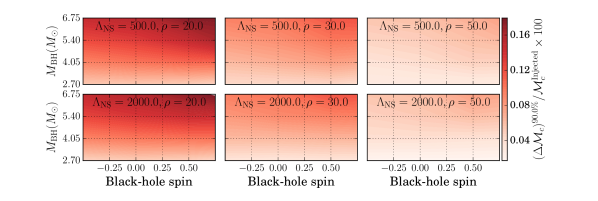
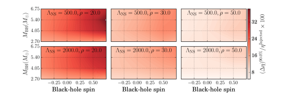
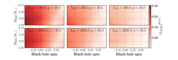
In Fig. 13, we show how precisely can we measure non-tidal NSBH parameters using BBH templates. The three panels correspond to (top), (middle), and (bottom), and show the width of these credible intervals as a function of BH mass/spin (within each sub-panel), and NS properties, i.e. (downwards in each column) 181818We restrict NS mass to and its spin to zero. Varying its tidal deformability does not significantly change the measurement uncertainties for non-tidal binary parameters, as is evident from comparing the two rows in each panel of Fig. 13.. From the left-most column, we find that: (i) at the chirp mass is measured remarkably well - to a precision of of its true value, and (ii) so is . (iii) The dimensionless mass-ratio is determined more loosely, with uncertainty. If the signal is even louder (), all three measurements gain further precision, especially , for which the relative errors shrink down to single-digit percents. We remind ourselves that these results do not tell the full story since the precision of a measurement is only meaningful if the measurement is accurate to begin with. In our case there are tidal effects that have not been incorporated into our search (BBH) templates, which can lead to a systematic bias in parameter recovery. We refer the reader to Sec. III for a comparative study of both systematic and statistical errors.
Appendix B Illustrations of Bayesian posteriors
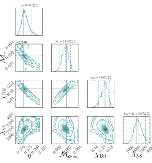
In Fig. 14 we show the correlation of mass, spin, and tidal parameter measurements. We keep the binary parameters as in Fig. 5, with , and set (left panel) or (right panel). We find that the measurement of is weakly degenerate with other parameters, and at realistic SNRs it would improve by a few tens of percent if we knew non-tidal parameters to better accuracy. The predominant factor that would enhance the measurement accuracy for is nevertheless the signal strength. Only when can we expect measurement to be limited by its degeneracy with non-tidal parameters (at a factor of few level), as also reported by previous studies Lackey et al. (2014).
Appendix C Phenomenology of measurement errors
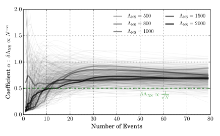
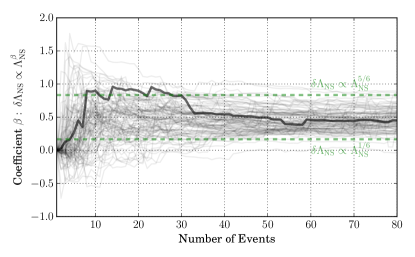
Here, we quantitatively explore the dependence of our statistical uncertainties for on the number of events, as well as on the true NS deformability itself. First, we will focus on the dependence on . We assume a power-law dependence of the form . For each of the populations for each of , we compute the exponent as a function of the number of observed events , and show it in Fig. 15. There are curves on the figure, with one highlighted for each value of population’s . These highlighted values are only special in the sense that they correspond to populations discussed earlier in this section (c.f. Fig. 8-9). We immediately observe two things, (i) there is a globally similar dependence on for all populations, and (ii) information accumulates faster than . In fact, we find that if , lines in the range . Next, we focus on the dependence of on of the population itself. As suggested by Fisher-matrix studies Lackey et al. (2014), and as for , we assume the form . From each set of populations with a given value, we draw one at random, and form a set of similarly drawn populations, one for each of . With each set, we determine for different number of observed events . In all, we make independent population sets and show the value of measured from each in Fig. 16. We find that the assumed relation gets fairly robust for larger values of , with converging to . The fact that implies that the relative error decreases with increasing , while the absolute error increases. From these results, we conclude that the measurement uncertainty for after observations is
| (17) |
We also find that while these results are inferred from paradigm A populations, paradigm B gives very similar results.
Appendix D Choice of underlying BBH model in LEA
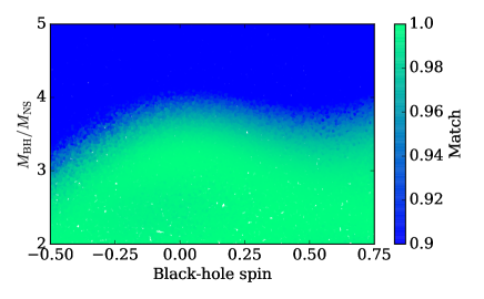
The waveform model used in this paper is a variant of those calibrated in Ref Lackey et al. (2014). In that work, the authors also calibrate a tidal prescription with the phenomenological model IMRPhenomC Santamaría et al. (2010) as the base BBH model. Previous work Kumar et al. (2015, 2016) has shown that IMRPhenomC can exhibit pathological behavior for mass-ratios and/or non-zero black hole spins. We compute noise-weighted inner-products between the two variants for points sampled over the NSBH parameter space, and show the results in Fig. 17. We restrict the comparison to frequencies that are affected by the tidal disruption of the NS, by integrating the inner-products from Hz (where is expressed in seconds (S, see Eq. (32-34) of Lackey et al. (2014)). We find that the differences between the two variants of LEA+ have mismatches of a few percent, while the tidal corrections contribute at a sub-percent level. We conclude that the differences of the underlying BBH model in LEA+ dominate over its tidal calibration, and since SEOBNRv2 has been shown to be more reliable than IMRPhenomC Kumar et al. (2015, 2016), we recommend the use of SEOBNRv2-based LEA+ in upcoming LIGO-Virgo analyses.
References
References
- Shoemaker (2010) D. Shoemaker (LIGO Collaboration), “Advanced LIGO anticipated sensitivity curves,” (2010), LIGO Document T0900288-v3.
- Abbott et al. (2016a) B. P. Abbott et al. (LIGO Scientific Collaboration, Virgo Collaboration), Phys. Rev. Lett. 116, 061102 (2016a), arXiv:1602.03837 [gr-qc] .
- The Virgo Collaboration (2009) The Virgo Collaboration, “Advanced Virgo Baseline Design,” (2009), [VIR-0027A-09].
- Acernese et al. (2015) F. Acernese et al. (Virgo Collaboration), Class. Quantum Grav. 32, 024001 (2015), arXiv:1408.3978 [gr-qc] .
- Aso et al. (2013) Y. Aso, Y. Michimura, K. Somiya, M. Ando, O. Miyakawa, T. Sekiguchi, D. Tatsumi, and H. Yamamoto (The KAGRA Collaboration), Phys. Rev. D 88, 043007 (2013), arXiv:1306.6747 [gr-qc] .
- Somiya (2012) K. Somiya (KAGRA Collaboration), Class. Quantum Grav. 29, 124007 (2012), arXiv:1111.7185 [gr-qc] .
- Unnikrishnan (2013) C. S. Unnikrishnan, International Journal of Modern Physics D 22, 1341010 (2013).
- Timmes et al. (1996) F. X. Timmes, S. E. Woosley, and T. A. Weaver, Astrophys. J. 457, 834 (1996), arXiv:astro-ph/9510136 [astro-ph] .
- Fryer (1999) C. L. Fryer, Astrophys. J. 522, 413 (1999), arXiv:astro-ph/9902315 [astro-ph] .
- Woosley et al. (2002) S. E. Woosley, A. Heger, and T. A. Weaver, Rev. Mod. Phys. 74, 1015 (2002).
- Belczynski et al. (2010a) K. Belczynski, T. Bulik, C. L. Fryer, A. Ruiter, F. Valsecchi, J. S. Vink, and J. R. Hurley, apj 714, 1217 (2010a), arXiv:0904.2784 [astro-ph.SR] .
- Belczynski et al. (2010b) K. Belczynski, M. Dominik, T. Bulik, R. O’Shaughnessy, C. Fryer, and D. E. Holz, Astrophys. J. Lett. 715, L138 (2010b), arXiv:1004.0386 [astro-ph.HE] .
- Dominik et al. (2015) M. Dominik, E. Berti, R. O’Shaughnessy, I. Mandel, K. Belczynski, C. Fryer, D. Holz, T. Bulik, and F. Pannarale, Astrophys. J. 806, 263 (2015), arXiv:1405.7016 [astro-ph.HE] .
- Belczynski et al. (2007) K. Belczynski, V. Kalogera, F. A. Rasio, R. E. Taam, and T. Bulik, Astrophys.J. 662, 504 (2007), arXiv:astro-ph/0612032 [astro-ph] .
- Fryer et al. (2012) C. L. Fryer, K. Belczynski, G. Wiktorowicz, M. Dominik, V. Kalogera, and D. E. Holz, Astrophys. J. 749, 91 (2012), arXiv:1110.1726 [astro-ph.SR] .
- Wex and Kopeikin (1999) N. Wex and S. Kopeikin, Astrophys. J. 514, 388 (1999), arXiv:astro-ph/9811052 [astro-ph] .
- Narayan et al. (1991) R. Narayan, T. Piran, and A. Shemi, Astrophys. J. 379, L17 (1991).
- Mandel et al. (2015) I. Mandel, C.-J. Haster, M. Dominik, and K. Belczynsk, (2015), 10.1093/mnrasl/slv054, arXiv:1503.03172 [astro-ph.HE] .
- Abbott et al. (2016b) B. P. Abbott et al. (Virgo, LIGO Scientific), (2016b), arXiv:1602.03842 [astro-ph.HE] .
- Psaltis et al. (2010) D. Psaltis, M. van der Klis, T. Strohmayer, L. Bildsten, J. McClintock, R. Remillard, P. Charles, M. Coe, J. Heise, J. in ’t Zand, V. Kaspi, M. Roberts, A. Harding, F. Verbunt, W. Lewin, R. Fender, E. Kuulkers, A. Norton, A. Schwope, B. Warner, P. Kahabka, E. van den Heuvel, G. Fabbiano, N. White, A. King, P. Woods, C. Thompson, K. Hurley, R. Sari, S. Djorgovski, and T. Tauris, in Compact Stellar X-ray Sources, edited by M. v. d. K. Walter Lewin (Cambridge University Press, 2010) p. 708.
- Remillard and McClintock (2006) R. A. Remillard and J. E. McClintock, Ann. Rev. Astron. Astrophys. 44, 49 (2006), arXiv:astro-ph/0606352 [astro-ph] .
- Fragos et al. (2010) T. Fragos, M. Tremmel, E. Rantsiou, and K. Belczynski, (2010), arXiv:1001.1107 [astro-ph.HE] .
- Manchester et al. (2005) R. N. Manchester, G. B. Hobbs, A. Teoh, and M. Hobbs, Astron. J. 129, 1993 (2005), arXiv:astro-ph/0412641 [astro-ph] .
- Lattimer (2012) J. M. Lattimer, Ann.Rev.Nucl.Part.Sci. 62, 485 (2012), arXiv:1305.3510 [nucl-th] .
- Margon et al. (1971) B. Margon, M. Lampton, S. Bowyer, and R. Cruddace, Astrophys. J. Lett. 169, L23 (1971).
- Bond et al. (2002) H. E. Bond, R. L. White, R. H. Becker, and M. S. O’Brien, Publ. Astron. Soc. Pac. 114, 1359 (2002), arXiv:astro-ph/0208383 [astro-ph] .
- Hulse and Taylor (1975) R. A. Hulse and J. H. Taylor, Astrophys. J. 195, L51 (1975).
- Taylor and Weisberg (1982) J. H. Taylor and J. M. Weisberg, Astrophys. J. 253, 908 (1982).
- Weisberg et al. (2010) J. Weisberg, D. Nice, and J. Taylor, Astrophys.J. 722, 1030 (2010), arXiv:1011.0718 [astro-ph.GA] .
- Janka et al. (1999) H.-T. Janka, T. Eberl, M. Ruffert, and C. L. Fryer, Astrophys. J. 527, L39 (1999), astro-ph/9908290 .
- Fryer et al. (2015) C. L. Fryer, F. G. Oliveira, J. A. Rueda, and R. Ruffini, Phys. Rev. Lett. 115, 231102 (2015), arXiv:1505.02809 [astro-ph.HE] .
- Abadie et al. (2010) J. Abadie, B. P. Abbott, R. Abbott, M. Abernathy, T. Accadia, F. Acernese, C. Adams, R. Adhikari, P. Ajith, B. Allen, and et al. (LIGO Scientific Collaboration, Virgo Collaboration), Class. Quantum Grav. 27, 173001 (2010), arXiv:1003.2480 [astro-ph.HE] .
- Eichler et al. (1989) D. Eichler, M. Livio, T. Piran, and D. N. Schramm, Nature 340, 126 (1989).
- Narayan et al. (1992) R. Narayan, B. Paczynski, and T. Piran, Astrophys. J. Lett. 395, L83 (1992), astro-ph/9204001 .
- Mochkovitch et al. (1993) R. Mochkovitch, M. Hernanz, J. Isern, and X. Martin, Nature 361, 236 (1993).
- Barthelmy et al. (2005) S. D. Barthelmy et al., Nature 438, 994 (2005), arXiv:astro-ph/0511579 [astro-ph] .
- Fox et al. (2005) D. B. Fox, D. A. Frail, P. A. Price, S. R. Kulkarni, E. Berger, T. Piran, A. M. Soderberg, S. B. Cenko, P. B. Cameron, A. Gal-Yam, M. M. Kasliwal, D.-S. Moon, F. A. Harrison, E. Nakar, B. P. Schmidt, B. Penprase, R. A. Chevalier, P. Kumar, K. Roth, D. Watson, B. L. Lee, S. Shectman, M. M. Phillips, M. Roth, P. J. McCarthy, M. Rauch, L. Cowie, B. A. Peterson, J. Rich, N. Kawai, K. Aoki, G. Kosugi, T. Totani, H.-S. Park, A. MacFadyen, and K. C. Hurley, Nature 437, 845 (2005), astro-ph/0510110 .
- Gehrels et al. (2005) N. Gehrels, C. L. Sarazin, P. T. O’Brien, B. Zhang, L. Barbier, S. D. Barthelmy, A. Blustin, D. N. Burrows, J. Cannizzo, J. R. Cummings, M. Goad, S. T. Holland, C. P. Hurkett, J. A. Kennea, A. Levan, C. B. Markwardt, K. O. Mason, P. Meszaros, M. Page, D. M. Palmer, E. Rol, T. Sakamoto, R. Willingale, L. Angelini, A. Beardmore, P. T. Boyd, A. Breeveld, S. Campana, M. M. Chester, G. Chincarini, L. R. Cominsky, G. Cusumano, M. de Pasquale, E. E. Fenimore, P. Giommi, C. Gronwall, D. Grupe, J. E. Hill, D. Hinshaw, J. Hjorth, D. Hullinger, K. C. Hurley, S. Klose, S. Kobayashi, C. Kouveliotou, H. A. Krimm, V. Mangano, F. E. Marshall, K. McGowan, A. Moretti, R. F. Mushotzky, K. Nakazawa, J. P. Norris, J. A. Nousek, J. P. Osborne, K. Page, A. M. Parsons, S. Patel, M. Perri, T. Poole, P. Romano, P. W. A. Roming, S. Rosen, G. Sato, P. Schady, A. P. Smale, J. Sollerman, R. Starling, M. Still, M. Suzuki, G. Tagliaferri, T. Takahashi, M. Tashiro, J. Tueller, A. A. Wells, N. E. White, and R. A. M. J. Wijers, Nature 437, 851 (2005), astro-ph/0505630 .
- Shibata et al. (2006) M. Shibata, M. D. Duez, Y. T. Liu, S. L. Shapiro, and B. C. Stephens, Phys. Rev. Lett. 96, 031102 (2006), arXiv:astro-ph/0511142 [astro-ph] .
- Paschalidis et al. (2015) V. Paschalidis, M. Ruiz, and S. L. Shapiro, Astrophys. J. 806, L14 (2015), arXiv:1410.7392 [astro-ph.HE] .
- Tanvir et al. (2013) N. R. Tanvir, A. J. Levan, A. S. Fruchter, J. Hjorth, R. A. Hounsell, K. Wiersema, and R. L. Tunnicliffe, Nature 500, 547 (2013), arXiv:1306.4971 [astro-ph.HE] .
- Foucart et al. (2015) F. Foucart, E. O’Connor, L. Roberts, M. D. Duez, R. Haas, L. E. Kidder, C. D. Ott, H. P. Pfeiffer, M. A. Scheel, and B. Szilagyi, Phys. Rev. D 91, 124021 (2015), arXiv:1502.04146 [astro-ph.HE] .
- Lovelace et al. (2013) G. Lovelace, M. D. Duez, F. Foucart, L. E. Kidder, H. P. Pfeiffer, M. A. Scheel, and B. Szilágyi, Class. Quantum Grav. 30, 135004 (2013), arXiv:1302.6297 [gr-qc] .
- Deaton et al. (2013) M. B. Deaton, M. D. Duez, F. Foucart, E. O’Connor, C. D. Ott, L. E. Kidder, C. D. Muhlberger, M. A. Scheel, and B. Szilagyi, Astrophys. J. 776, 47 (2013), arXiv:1304.3384 [astro-ph.HE] .
- Foucart (2012) F. Foucart, Phys. Rev. D 86, 124007 (2012), arXiv:1207.6304 [astro-ph.HE] .
- Foucart et al. (2013a) F. Foucart, L. Buchman, M. D. Duez, M. Grudich, L. E. Kidder, I. MacDonald, A. Mroue, H. P. Pfeiffer, M. A. Scheel, and B. Szilagyi, Phys. Rev. D 88, 064017 (2013a), arXiv:1307.7685 [gr-qc] .
- Foucart et al. (2014) F. Foucart, M. B. Deaton, M. D. Duez, E. O’Connor, C. D. Ott, R. Haas, L. E. Kidder, H. P. Pfeiffer, M. A. Scheel, and B. Szilagyi, Phys. Rev. D 90, 024026 (2014), arXiv:1405.1121 [astro-ph.HE] .
- Shibata and Taniguchi (2008) M. Shibata and K. Taniguchi, Phys. Rev. D77, 084015 (2008), arXiv:0711.1410 [gr-qc] .
- Ferrari et al. (2010) V. Ferrari, L. Gualtieri, and F. Pannarale, Phys. Rev. D 81, 064026 (2010), arXiv:0912.3692 [gr-qc] .
- Kawaguchi et al. (2015) K. Kawaguchi, K. Kyutoku, H. Nakano, H. Okawa, M. Shibata, and K. Taniguchi, Phys. Rev. D 92, 024014 (2015), arXiv:1506.05473 [astro-ph.HE] .
- Abbott et al. (2016c) B. P. Abbott et al. (LIGO Scientific Collaboration, Virgo Collaboration), Living Rev. Rel. 19 (2016c), 10.1007/lrr-2016-1, arXiv:1304.0670v3 [gr-qc] .
- Lee and Kluzniak (1999a) W. H. Lee and W. L. Kluzniak, Astroph. J. 526, 178 (1999a).
- Lee and Kluzniak (1999b) W. H. Lee and W. L. Kluzniak, Mon. Not. Roy. Astr. Soc. 308, 780 (1999b).
- Lee (2000) W. H. Lee, Mon. Not. Roy. Astr. Soc. 318, 606 (2000).
- Oechslin et al. (2007) R. Oechslin, H. T. Janka, and A. Marek, Astron. Astrophys. 467, 395 (2007), arXiv:astro-ph/0611047 .
- Read et al. (2009) J. S. Read, B. D. Lackey, B. J. Owen, and J. L. Friedman, Phys. Rev. D79, 124032 (2009), arXiv:0812.2163 [astro-ph] .
- Markakis et al. (2010) C. Markakis, J. S. Read, M. Shibata, K. Uryu, J. D. E. Creighton, and J. L. Friedman, in On recent developments in theoretical and experimental general relativity, astrophysics and relativistic field theories. Proceedings, 12th Marcel Grossmann Meeting on General Relativity, Paris, France, July 12-18, 2009. Vol. 1-3 (2010) pp. 743–745, arXiv:1008.1822 [gr-qc] .
- Markakis et al. (2009) C. Markakis, J. S. Read, M. Shibata, K. Uryu, J. D. Creighton, et al., J. Phys. Conf. Ser. 189, 012024 (2009), arXiv:1110.3759 [gr-qc] .
- Stergioulas et al. (2011) N. Stergioulas, A. Bauswein, K. Zagkouris, and H.-T. Janka, Mon. Not. Roy. Astr. Soc. 418, 427 (2011), arXiv:1105.0368 [gr-qc] .
- East et al. (2012) W. E. East, F. Pretorius, and B. C. Stephens, Phys. Rev. D 85, 124009 (2012), arXiv:1111.3055 [astro-ph.HE] .
- Lackey and Wade (2015) B. D. Lackey and L. Wade, Phys. Rev. D 91, 043002 (2015), arXiv:1410.8866 [gr-qc] .
- Wade et al. (2014) L. Wade, J. D. E. Creighton, E. Ochsner, B. D. Lackey, B. F. Farr, et al., Phys. Rev. D 89, 103012 (2014), arXiv:1402.5156 [gr-qc] .
- Bauswein et al. (2014) A. Bauswein, N. Stergioulas, and H.-T. Janka, Phys. Rev. D 90, 023002 (2014), arXiv:1403.5301 [astro-ph.SR] .
- Flanagan and Hinderer (2008) É. É. Flanagan and T. Hinderer, Phys. Rev. D 77, 021502 (2008), arXiv:0709.1915 .
- Kyutoku et al. (2010) K. Kyutoku, M. Shibata, and K. Taniguchi, Phys. Rev. D 82, 044049 (2010), arXiv:1008.1460 [astro-ph.HE] .
- Lackey et al. (2014) B. D. Lackey, K. Kyutoku, M. Shibata, P. R. Brady, and J. L. Friedman, Phys. Rev. D 89, 043009 (2014), arXiv:1303.6298 [gr-qc] .
- Pannarale et al. (2015a) F. Pannarale, E. Berti, K. Kyutoku, B. D. Lackey, and M. Shibata, (2015a), arXiv:1509.06209 [gr-qc] .
- Vines et al. (2011) J. Vines, É. É. Flanagan, and T. Hinderer, Phys. Rev. D 83, 084051 (2011), arXiv:1101.1673 [gr-qc] .
- Maselli et al. (2013) A. Maselli, L. Gualtieri, and V. Ferrari, Phys. Rev. D 88, 104040 (2013), arXiv:1310.5381 [gr-qc] .
- Barkett et al. (2016) K. Barkett, M. A. Scheel, R. Haas, C. D. Ott, S. Bernuzzi, D. A. Brown, B. Szilágyi, J. D. Kaplan, J. Lippuner, C. D. Muhlberger, F. Foucart, and M. D. Duez, Phys. Rev. D 93, 044064 (2016), arXiv:1509.05782 [gr-qc] .
- Yagi and Yunes (2014) K. Yagi and N. Yunes, Phys. Rev. D 89, 021303 (2014), arXiv:1310.8358 [gr-qc] .
- Lackey et al. (2012) B. D. Lackey, K. Kyutoku, M. Shibata, P. R. Brady, and J. L. Friedman, Phys. Rev. D 85, 044061 (2012), arXiv:1109.3402 [astro-ph.HE] .
- Vallisneri (2008) M. Vallisneri, Phys. Rev. D77, 042001 (2008), arXiv:gr-qc/0703086 [GR-QC] .
- Bailyn et al. (1998) C. D. Bailyn, R. K. Jain, P. Coppi, and J. A. Orosz, Astrophys. J. 499, 367 (1998), arXiv:astro-ph/9708032 [astro-ph] .
- Kalogera and Baym (1996) V. Kalogera and G. Baym, Astrophys. J. 470, L61 (1996), arXiv:astro-ph/9608059 [astro-ph] .
- Kreidberg et al. (2012) L. Kreidberg, C. D. Bailyn, W. M. Farr, and V. Kalogera, Astroph.J. 757, 36 (2012), arXiv:1205.1805 [astro-ph.HE] .
- Littenberg et al. (2015) T. B. Littenberg, B. Farr, S. Coughlin, V. Kalogera, and D. E. Holz, (2015), arXiv:1503.03179 [astro-ph.HE] .
- Tolman (1939) R. C. Tolman, Phys. Rev. 55, 364 (1939).
- Oppenheimer and Volkoff (1939) J. R. Oppenheimer and G. M. Volkoff, Phys. Rev. 55, 374 (1939).
- Tolman (1934) R. C. Tolman, Proceedings of the National Academy of Science 20, 169 (1934).
- Del Pozzo et al. (2013) W. Del Pozzo, T. G. F. Li, M. Agathos, C. Van Den Broeck, and S. Vitale, Phys. Rev. Lett. 111, 071101 (2013), arXiv:1307.8338 [gr-qc] .
- Abadie et al. (2010) J. Abadie et al. (LIGO Scientific Collaboration), Class. Quantum Grav. 27, 173001 (2010), arXiv:1003.2480 [gr-qc] .
- Pannarale et al. (2015b) F. Pannarale, E. Berti, K. Kyutoku, B. D. Lackey, and M. Shibata, Phys. Rev. D 92, 084050 (2015b), arXiv:1509.00512 [gr-qc] .
- Agathos et al. (2015) M. Agathos, J. Meidan, W. D. Pozzo, T. G. F. Li, M. Tompitak, J. Veitch, S. Vitale, and C. V. D. Broeck, Phys. Rev. D 92, 023012 (2015), arXiv:1503.05405 [gr-qc] .
- Taracchini et al. (2012) A. Taracchini, Y. Pan, A. Buonanno, E. Barausse, M. Boyle, T. Chu, G. Lovelace, H. P. Pfeiffer, and M. A. Scheel, Phys. Rev. D 86, 024011 (2012), arXiv:1202.0790 [gr-qc] .
- Buonanno and Damour (1999) A. Buonanno and T. Damour, Phys. Rev. D 59, 084006 (1999), arXiv:gr-qc/9811091 [gr-qc] .
- Taracchini et al. (2014) A. Taracchini, A. Buonanno, Y. Pan, T. Hinderer, M. Boyle, D. A. Hemberger, L. E. Kidder, G. Lovelace, A. H. Mroue, H. P. Pfeiffer, M. A. Scheel, B. Szilagyi, N. W. Taylor, and A. Zenginoglu, Phys. Rev. D 89 (R), 061502 (2014), arXiv:1311.2544 [gr-qc] .
- Pürrer (2015) M. Pürrer, (2015), arXiv:1512.02248 [gr-qc] .
- Kumar et al. (2015) P. Kumar, K. Barkett, S. Bhagwat, N. Afshari, D. A. Brown, G. Lovelace, M. A. Scheel, and B. Szilágyi, Phys. Rev. D 92, 102001 (2015), arXiv:1507.00103 [gr-qc] .
- Kumar et al. (2016) P. Kumar, T. Chu, H. Fong, H. P. Pfeiffer, M. Boyle, D. A. Hemberger, L. E. Kidder, M. A. Scheel, and B. Szilagyi, Phys. Rev. D93, 104050 (2016), arXiv:1601.05396 [gr-qc] .
- (91) L. S. Collaboration, “LSC Algorithm Library software packages lal, lalwrapper, and lalapps,” .
- Pürrer et al. (2015) M. Pürrer, M. Hannam, and F. Ohme, (2015), arXiv:1512.04955 [gr-qc] .
- Foreman-Mackey et al. (2013) D. Foreman-Mackey, D. W. Hogg, D. Lang, and J. Goodman, arXiv 125, 306 (2013), arXiv:1202.3665 [astro-ph.IM] .
- Gelman and Rubin (1992) A. Gelman and D. B. Rubin, Statist. Sci. 7, 457 (1992).
- Puerrer et al. (2016) M. Puerrer et al., (2016), in preparation.
- Sathyaprakash and Schutz (2009) B. S. Sathyaprakash and B. F. Schutz, Living Rev. Rel. 12, 2 (2009), arXiv:0903.0338 [gr-qc] .
- Foucart et al. (2012) F. Foucart, M. D. Duez, L. E. Kidder, M. A. Scheel, B. Szilágyi, and S. A. Teukolsky, Phys. Rev. D 85, 044015 (2012), arXiv:1111.1677 [gr-qc] .
- Pannarale et al. (2011) F. Pannarale, L. Rezzolla, F. Ohme, and J. S. Read, Phys. Rev. D 84, 104017 (2011), arXiv:1103.3526 [astro-ph.HE] .
- Kiziltan et al. (2013) B. Kiziltan, A. Kottas, M. De Yoreo, and S. E. Thorsett, Astrophys. J. 778, 66 (2013).
- Mandel (2010) I. Mandel, Phys. Rev. D81, 084029 (2010), arXiv:0912.5531 [astro-ph.HE] .
- Chatziioannou et al. (2015) K. Chatziioannou, K. Yagi, A. Klein, N. Cornish, and N. Yunes, Phys. Rev. D 92, 104008 (2015), arXiv:1508.02062 [gr-qc] .
- Abbott et al. (2016d) B. P. Abbott et al. (Virgo, LIGO Scientific), Phys. Rev. Lett. 116, 061102 (2016d), arXiv:1602.03837 [gr-qc] .
- Abbott et al. (2016e) B. P. Abbott et al. (Virgo, LIGO Scientific), Phys. Rev. Lett. 116, 241103 (2016e), arXiv:1606.04855 [gr-qc] .
- Abbott et al. (2016f) B. P. Abbott et al. (Virgo, LIGO Scientific), (2016f), arXiv:1607.07456 [astro-ph.HE] .
- Abadie et al. (2012) J. Abadie, B. P. Abbott, R. Abbott, T. D. Abbott, M. Abernathy, T. Accadia, F. Acernese, C. Adams, R. Adhikari, C. Affeldt, and et al., Astron. Astrophys. 541, A155 (2012), arXiv:1112.6005 .
- Singer et al. (2014) L. P. Singer et al., Astrophys. J. 795, 105 (2014), arXiv:1404.5623 [astro-ph.HE] .
- Singer and Price (2016) L. P. Singer and L. R. Price, Phys. Rev. D93, 024013 (2016), arXiv:1508.03634 [gr-qc] .
- Pankow et al. (2015) C. Pankow, P. Brady, E. Ochsner, and R. O’Shaughnessy, Phys. Rev. D92, 023002 (2015), arXiv:1502.04370 [gr-qc] .
- Abbott et al. (2016g) B. P. Abbott et al. (InterPlanetary Network, DES, INTEGRAL, La Silla-QUEST Survey, MWA, Fermi-LAT, J-GEM, DEC, GRAWITA, Pi of the Sky, Fermi GBM, MASTER, Swift, iPTF, VISTA, ASKAP, SkyMapper, PESSTO, TOROS, Pan-STARRS, Virgo, Liverpool Telescope, BOOTES, LIGO Scientific, LOFAR, C2PU, MAXI), Astrophys. J. 826, L13 (2016g), arXiv:1602.08492 [astro-ph.HE] .
- Foucart et al. (2013b) F. Foucart, M. B. Deaton, M. D. Duez, L. E. Kidder, I. MacDonald, C. D. Ott, H. P. Pfeiffer, M. A. Scheel, B. Szilagyi, and S. A. Teukolsky, Phys. Rev. D 87, 084006 (2013b), arXiv:1212.4810 [gr-qc] .
- Hinderer et al. (2016) T. Hinderer et al., Phys. Rev. Lett. 116, 181101 (2016), arXiv:1602.00599 [gr-qc] .
- Santamaría et al. (2010) L. Santamaría, F. Ohme, P. Ajith, B. Brügmann, N. Dorband, M. Hannam, S. Husa, P. Mösta, D. Pollney, C. Reisswig, E. L. Robinson, J. Seiler, and B. Krishnan, Phys. Rev. D 82, 064016 (2010), arXiv:1005.3306 [gr-qc] .