Large-Scale Cosmic-Ray Anisotropy as a Probe of Interstellar Turbulence

Abstract

We calculate the large-scale cosmic-ray (CR) anisotropies predicted for a range of Goldreich-Sridhar (GS) and isotropic models of interstellar turbulence, and compare them with IceTop data. In general, the predicted CR anisotropy is not a pure dipole; the cold spots reported at $400$ TeV and $2\,$PeV are consistent with a GS model that contains a smooth deficit of parallel-propagating waves and a broad resonance function, though some other possibilities cannot, as yet, be ruled out. In particular, isotropic fast magnetosonic wave turbulence can match the observations at high energy, but cannot accommodate an energy dependence in the shape of the CR anisotropy. Our findings suggest that improved data on the large-scale CR anisotropy could provide a valuable probe of the properties — notably the power-spectrum — of the interstellar turbulence within a few tens of parsecs from Earth.

1. Introduction

In this paper, we focus on the possible role of turbulence in the local interstellar medium, within about a cosmic-ray (CR) mean free path from Earth, in shaping the large-scale or global anisotropy of CRs of energy between 100 TeV and a few PeV, i.e., on features in their angular distribution that are larger than several tens of degrees in size. Aside from a small distortion attributable to the draping of magnetic field lines around the heliosphere, Schwadron et al. (2014) find that the direction of the global anisotropy of TeV CR is compatible with that of the magnetic field as deduced both from the IBEX ribbon, and from polarization of optical starlight from stars within a few tens of parsecs (Frisch et al., 2012, 2015). In principle, this could be due to a coincidental alignment of the CR density gradient and the field direction, but we interpret it as supporting the view that CRs diffuse mainly along field lines, rather than across them, in which case the density gradient is not strongly constrained. Although explanations have been advanced for small-scale anisotropies that can arise from the configuration of the interstellar magnetic field (Giacinti & Sigl, 2012; Battaner et al., 2015; López-Barquero et al., 2016), both the amplitude and the shape of the global anisotropy remain unexplained. Until now, the amplitude has attracted most of the attention (Blasi & Amato, 2012; Pohl & Eichler, 2013; Kumar & Eichler, 2014; Mertsch & Funk, 2015). Here we are primarily concerned with the shape and its potential to provide information on the turbulent component of the local field.

Anisotropies in the arrival directions of TeV–PeV CRs have been detected in both hemispheres and at multiple angular scales by several observatories (a review of experimental results is presented in Di Sciascio & Iuppa, 2014). However, the most useful data sets for our purposes are those published by the IceCube/IceTop collaboration (Aartsen et al., 2013, 2016) for high-energy ($\gtrsim 100$ TeV) CRs, because these data are free from features caused by heliospheric fields, which demand a different explanation (Desiati & Lazarian, 2013; Drury, 2013).

A dipole anisotropy, such as would be expected from the Compton-Getting effect if the Solar System were drifting through an isotropic distribution of CRs, is clearly ruled out by the data (Aartsen et al., 2013, 2016), at least for CRs of energy $\gtrsim 100$ TeV. Instead, IceTop has detected a relatively small cold spot in its field of view, whereas the CR flux in the rest of the observed sky is much more isotropic. The typical size of the cold spot is $\approx 30^{\circ}$ for the data set with 400 TeV median energy, and $\approx 40^{\circ}$ at 2 PeV (Aartsen et al., 2013). A dipole anisotropy would produce a larger cold spot, as well as an undetected maximum in the CR flux in the observed part of the sky at the opposite value of the cold spot’s right ascension.

Although the partial sky coverage of IceTop/IceCube can give rise to artefacts (e.g. Ahlers et al., 2016), we take these data at face value and address the question of how they can be used to constrain the nature of the turbulence underlying CR transport. Although attempts to go beyond the pure dipole description have been made — e.g., by Zhang et al. (2014), who represented the large-scale anisotropy phenomenologically as a sum of Legendre polynomials — a quantitative approach to the question that specifically relates it to turbulence models has, so far, not been attempted.

In this paper, we compute the anisotropies that arise from an anisotropic spectrum of Alfvén waves of Goldreich-Sridhar type (Sridhar & Goldreich, 1994; Goldreich & Sridhar, 1995), as well as from an isotropic distribution of fast magnetosonic modes with a power-spectrum compatible with that found in the MHD simulations of Cho & Lazarian (2002). The pitch-angle scattering rates for these models have been calculated previously by, for example, Chandran (2000) and Yan & Lazarian (2002, 2004, 2008), but these authors did not use them to predict the CR anisotropy. Each hypothesis necessarily contains input of a phenomenological nature concerning the precise functional form of the anisotropy, as well as the so-called “resonance function”. We find that the data yield constraints on these inputs, as well as on quantities such as the Alfvén speed and the outer length scale of the turbulent spectrum. Our approach is similar in spirit to that of Malkov et al. (2010), who addressed the problem of anisotropies on small angular scales. The main methodological differences are that we use the full general solution of the equation for CR pitch-angle diffusion, compute the angular diffusion coefficients numerically, and use more recent data on the direction of the local magnetic field.

In Section 2 the general expression for the CR anisotropy as a function of the CR pitch-angle is derived. Section 3 presents calculations of this anisotropy, both for Alfvénic turbulence with an anisotropic Goldreich-Sridhar power-spectrum, and for compressible turbulence with isotropic fast magnetosonic modes. We then discuss the implications of our findings and the validity of our assumptions in Section 4, and summarize our main results in Section 5.

2. CR anisotropy and pitch-angle diffusion

The CR anisotropy at Earth is shaped by our local environment, which, according to studies of the polarization of optical light from nearby stars (Frisch et al., 2012, 2015), contains a magnetic field that is coherent in direction over a few tens of parsecs — see Section 4 for a discussion on the nature and direction of this field. Since the Larmor radius of TeV–PeV CRs, $r_{\rm L}\sim(10^{-4}-1)$ pc, is relatively small, this field is viewed by them as a quasi-homogeneous field, that dominates their propagation in the vicinity of the Solar System. As noted above, this is confirmed by the fact that the observed CR anisotropy direction is compatible with the direction of the local field. Therefore, in the following, we adopt a model in which CRs propagate in a magnetic flux tube of length between $\sim 10$ and a few times $10$ parsecs. Schwadron et al. (2014) find that the energy density in turbulence on scales of the Larmor radii of TeV–PeV CRs is quite small compared to that in the coherent field, and, moreover, note that cross-field diffusion is not expected to influence the global anisotropy. Therefore, we assume that the transport of CRs is described by pitch-angle diffusion along a local, uniform flux tube, and look for a stationary solution of the transport equation governing the pitch-angle distribution $f(x,\mu)$ of CRs (e.g., Vedenov et al., 1962; Malkov et al., 2010; Malkov & Sagdeev, 2015):

$$\mu v\frac{\partial f}{\partial x}=\frac{\partial}{\partial\mu}\left(D_{\mu\mu}\frac{\partial f}{\partial\mu}\right)\;,$$ (1)

where $\mu$ is the cosine of the CR pitch-angle $\vartheta$, $v$ the CR velocity (assumed here to equal the speed of light), $x$ the spatial coordinate along the flux tube, and $D_{\mu\mu}$ is the pitch-angle diffusion coefficient, which vanishes at $\mu=\pm 1$ and is positive definite in the range $-1<\mu<1$.

2.1. CR anisotropy

A standard approach to equations of the form of (1) is to separate the variables and expand in eigenfunctions (e.g., Bethe et al., 1938):

$$f(x,\mu)=\sum_{\rm i}a_{\rm i}e^{\Lambda_{\rm i}x/v}Q_{\rm i}(\mu)\;,$$ (2)

where the eigenvalues $\Lambda_{\rm i}$ and eigenfunctions $Q_{\rm i}(\mu)$ obey

$$\Lambda_{\rm i}\mu Q_{\rm i}=\frac{\partial}{\partial\mu}D_{\mu\mu}\frac{\partial}{\partial\mu}Q_{\rm i}\;,$$ (3)

together with boundary conditions on $Q_{\rm i}$ that ensure regularity and single-valuedness, i.e., $\pm\Lambda_{\rm i}Q_{\rm i}=-D^{\prime}_{\mu\mu}Q^{\prime}_{\rm i}$ at $\mu=\pm 1$ (where ^′ means differentiation with respect to $\mu$). However, this method is not guaranteed to work, because the weighting function, $\mu$, on the left-hand side of Eq. (3) has a zero within the relevant range. The problem then arises that that the $Q_{\rm i}$ do not form a complete set of functions on the range $-1\leq\mu\leq 1$. Fortunately, this can be remedied simply by adding a special solution, the diffusion solution, to the expansion in Eq. (2) (Fisch & Kruskal, 1980):

$$f_{\rm diff}=a_{\rm diff}\left[x+g(\mu)\right]\;,$$ (4)

where $a_{\rm diff}$ is a constant and $g(\mu)$ is a solution of

$$\frac{\partial}{\partial\mu}D_{\mu\mu}\frac{\partial}{\partial\mu}g=v\mu\;,$$ (5)

that satisfies the regularity conditions at $\mu=\pm 1$. The general solution can then be written as:

$$f(x,\mu)=\sum_{\rm i}a_{\rm i}e^{\Lambda_{\rm i}x/v}Q_{\rm i}(\mu)+a_{\rm diff}\left[x+g(\mu)\right]\;,$$ (6)

and, because $g$ is defined to within an arbitrary, additive constant, we can impose the additional condition

$$\int_{-1}^{1}{\rm d}\mu\,g(\mu)=0\;.$$ (7)

Note that the $Q_{\rm i}$ are orthogonal with the weighting function $\mu$:

$$\int_{-1}^{1}{\rm d}\mu\,Q_{\rm i}\mu Q_{\rm j}=0\;,$$ (8)

for $\Lambda_{\rm i}\neq\Lambda_{\rm j}$, and $g$ is orthogonal to all the $Q_{\rm i}$ except for the isotropic eigenfunction $Q_{0}=1$ with eigenvalue $\Lambda_{0}=0$:

$$\int_{-1}^{1}{\rm d}\mu\,Q_{\rm i}\mu g=0\;,$$ (9)

for $\Lambda_{\rm i}\neq 0$. The eigenvalues themselves can be ordered such that $\Lambda_{\rm i+1}>\Lambda_{\rm i}$, and occur in pairs with opposite signs: $\Lambda_{\rm i}=-\Lambda_{\rm-i}$.

The energy $E$ of the CR enters this problem as a parameter: if the diffusion coefficient is a function of $E$, then so are $\Lambda_{\rm i}$, $Q_{\rm i}$, and $g$.

Let us assume that the Earth is located at $x=0$. We wish to impose boundary conditions “far” from the Earth and examine the anisotropy expected at Earth. First, note that the CR flux $\mathcal{S}$ is a conserved quantity: $d\mathcal{S}/dx=0$, since it is assumed that there are no sources of CR within the flux tube. Then, using (5), (6) and (8):

$$\mathcal{S}=\frac{v}{2}\int_{-1}^{1}{\rm d}\mu\,\mu f=-\frac{a_{\rm diff}}{2}\int_{-1}^{1}{\rm d}\mu\,D_{\mu\mu}\left(g^{\prime}\right)^{2}\;.$$ (10)

Now consider boundaries at $x=\pm d$ ($d>0$), and impose a positive flux, so that $a_{\rm diff}<0$. This procedure is valid as long as there is a non-zero component of the global CR density gradient when projected onto the $x$-axis, whatever its origin — see Section 4 for a more detailed discussion of this point. In principle, the solution at the boundaries can contain the diffusive solution plus an arbitrary isotropic component, plus components that will either decay or grow exponentially as one moves from the boundary towards Earth. If $d$ is large, in the sense that

$$\textrm{exp}\left(-\Lambda_{\rm 1}d/v\right)\ll 1\,,$$ (11)

then it is clear from Eq. (6) that the terms with $\Lambda_{\rm i}>0$ are important only in a boundary layer close to $x=-d$, and those with $\Lambda_{\rm i}<0$ are important only in the corresponding layer close to $x=d$. In this case, within most of the flux tube, including the position of the Earth, the solution is accurately represented by

$$f(x,\mu)=a_{0}+a_{\rm diff}\left[x+g(\mu)\right]\;.$$ (12)

The CR anisotropy in this region is proportional to $g$, and equals $a_{\rm diff}\,g(\mu)/a_{0}$ at Earth. A spatial diffusion coefficient, $\kappa_{\parallel}$ and its associated mean free path $\lambda_{\parallel}$ can be defined via Fick’s Law:

$$\kappa_{\parallel} =-\frac{\mathcal{S}}{\partial f/\partial x}$$

$$=\frac{1}{2}\int_{-1}^{1}{\rm d}\mu D_{\mu\mu}\left(g^{\prime}\right)^{2}$$ (13)

$$\lambda_{\parallel} =\frac{3}{v}\kappa_{\parallel}\,.$$ (14)

Equation (5) with the condition (7) can be solved to give

$$g(\mu) =-\frac{v}{2}\int_{0}^{\mu}{\rm d}\mu^{\prime}\,\frac{1-\mu^{\prime 2}}{D_{\mu^{\prime}\mu^{\prime}}}\,,$$ (15)

so that

$$\kappa_{\parallel} =\frac{v^{2}}{4}\int_{0}^{1}{\rm d}\mu\frac{\left(1-\mu^{2}\right)^{2}}{D_{\mu\mu}}$$ (16)

(cf. Hasselmann & Wibberenz, 1970).

Note that Eq. (11) is a sufficient condition for the accuracy of (12), which is usually called the “diffusion approximation”. There is, in particular, no formal restriction on the size of the mean free path $\lambda_{\parallel}$, which can substantially exceed the length $2d$ of the flux tube without jeopardising the applicability of the diffusion approximation. The relationship between $\lambda_{\parallel}$ and $\Lambda_{1}$ depends on the functional form of the pitch-angle diffusion coefficient $D_{\mu\mu}$. In the following, we evaluate these quantities using the method outlined in Kirk et al. (2000). Since we consider only $D_{\mu\mu}$ which are even functions of $\mu$, the anisotropy is an odd function. Furthermore, the properties of the local turbulence constrain only the shape of the anisotropy, whereas its amplitude depends on the externally imposed flux. Therefore, we work with the normalized quantity

$$\hat{g}(\mu) =g(\mu)/g(1)$$ (17)

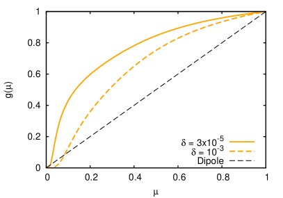
on the range $0\leq\mu\leq 1$, and, in order to simplify the notation, will drop the circumflex from here onwards. In the special case of isotropic pitch-angle diffusion, $D_{\mu\mu}\propto 1-\mu^{2}$, one finds $\Lambda_{1}/v=7.26/\lambda_{\parallel}$. This is also the only case in which the anisotropy has exactly the form of a dipole: $g(\mu)=\mu$.

2.2. Pitch-angle diffusion

In the so-called “quasi-linear” approach, the pitch-angle diffusion coefficient is computed from the expression (e.g. Kulsrud & Pearce, 1969; Völk, 1973, 1975):

$$D_{\mu\mu} =\Omega^{2}\left(1-\mu^{2}\right)\int{\rm d}^{3}k\int_{0}^{\infty}{\rm d}\tau$$

$$\sum_{n=-\infty}^{\infty}\bigg{(}\frac{n^{2}J_{\rm n}^{2}(z)}{z^{2}}M_{\rm A}({\bf k},\tau)+\frac{k_{\parallel}^{2}J_{\rm n}^{\prime 2}(z)}{k^{2}}M_{\rm P}({\bf k},\tau)\bigg{)}\;,$$ (18)

where $\Omega$ is the Larmor frequency, $k_{\parallel}$ and $k_{\perp}$ are the components of k parallel and perpendicular to the local field lines, respectively, $z=k_{\perp}l\varepsilon\sqrt{1-\mu^{2}}$, where $l$ is the outer scale of the turbulence and $\varepsilon=v/(l\Omega)=r_{\rm L}/l$, and $J_{\rm n}(z)$ is a Bessel function of the first kind (^′ denotes a derivative with respect to the argument $z$).

The quantities $M_{\rm A}$ and $M_{\rm P}$ represent normalized wave power spectra. Following Chandran (2000), they can be derived from the spatial Fourier transform of the turbulent magnetic field ${\bf B}_{1,{\rm w}}({\bf k},t)$, where ${\bf k}$ is the wave-vector and $t$ the time:

$$M_{\rm w}({\bf k},\tau)=\langle{\bf B}_{\rm 1,w}({\bf k},t)\cdot{\bf B}_{\rm 1,w}^{\ast}({\bf k},t+\tau)\rangle/B_{0}^{2}\;.$$ (19)

Here, $B_{0}$ is the regular part of the local (within a few tens of parsecs) magnetic field, ${\rm w}\in\{{\rm A,P}\}$ denotes the wave mode, and $\langle\dots\rangle$ represents an ensemble-average. These quantities can also be defined in terms of time-averages over a single realisation of stationary turbulence, but the distinction is unimportant for our investigation, since they enter our calculations only in the normalized energy spectra and resonance functions defined in section 2.2.1, for which we adopt phenomenological descriptions. Again following Chandran (2000), we assume equipartition between the magnetic and kinetic energy densities, and equal energy densities in each wave mode, and chose the normalization of the fluctuations such that the total magnetic energy in turbulence of wavelength shorter than that of the outer scale, $l$, equals that in the ambient field $B_{0}$. Shear Alfvén waves, which are described by $M_{\rm A}$, do not possess a fluctuating component of the magnetic field in the direction parallel to the ambient field and, therefore, do not contribute to the $n=0$ term in the summation. On the other hand, the slow and fast modes in compressible MHD, as well as the pseudo-Alfvén mode in the model of incompressible MHD do have such a component, and a corresponding contribution to this term. Their power spectra are described by $M_{\rm P}$. Below, we consider a compressible turbulence model in which the fast mode dominates over the slow mode, in which case we replace the suffix “P” by “F”. We also consider an incompressible model in which only the pseudo-Alfvén mode contributes to this term. In this case, because this mode can be considered as the analog of a slow mode, we replace “P” by “S”.

2.2.1 Resonance functions

In the following, $v_{\parallel}=v\mu$ and $v_{\perp}=v\sqrt{1-\mu^{2}}$ denote the components of the CR velocity parallel and perpendicular to the ambient magnetic field, and $\omega$ is the angular frequency of the waves. Expression (18) for $D_{\mu\mu}$ can be written in terms of a resonance function $R_{\rm n}(k_{\parallel}v_{\parallel}-\omega+n\Omega)$ that incorporates the integral over $\tau$:

$$D_{\mu\mu}=\Omega^{2}\left(1-\mu^{2}\right)\int{\rm d}^{3}k\sum_{n=-\infty}^{\infty}\bigg{(}\frac{n^{2}J_{\rm n}^{2}(z)}{z^{2}}\mathcal{I}_{\rm A}({\bf k})$$ (20)

$$+\frac{k_{\parallel}^{2}J_{\rm n}^{\prime 2}(z)}{k^{2}}\mathcal{I}_{\rm S,F}({\bf k})\bigg{)}\times R_{\rm n}(k_{\parallel}v_{\parallel}-\omega+n\Omega)\,,$$

where $\mathcal{I}_{\rm A,S,F}$ are the normalized energy spectra corresponding to the power spectra $M_{\rm A,S,F}$.

In quasi-linear theory (e.g., Jokipii, 1966), the resonance function $R_{\rm n}$ is a delta function. The shortcomings of this theory, such as the $90^{\circ}$-scattering problem (Jones et al., 1978) are well known. We note that this theory cannot account for the CR anisotropy data: as we show in Section 3, a broad peak in $D_{\mu\mu}/(1-\mu^{2})$ around $\mu=0$ is essential to reproduce the flattening observed in the CR anisotropy data by IceTop and IceCube for CRs with pitch-angles around $\vartheta=90^{\circ}$. Therefore, in this study, we consider two generic, phenomenological resonance functions.

For the first type of resonance function, we choose a Breit-Wigner distribution:

$$R_{\rm n,1}(k_{\parallel}v_{\parallel}-\omega+n\Omega)$$

$$=\mathcal{R}e\left(\int_{0}^{\infty}{\rm d}\tau\,\textrm{e}^{-i(k_{\parallel}v_{\parallel}-\omega+n\Omega)\tau-\tau/\tau_{\rm w}}\right)$$

$$=\frac{\tau_{\rm w}^{-1}}{(k_{\parallel}v_{\parallel}-\omega+n\Omega)^{2}+\tau_{\rm w}^{-2}}\;$$ (21)

where the broadening of the resonance, described by $\tau_{\rm w}$ with $w\in{A,F}$, is assumed to be dominated by the Lagrangian correlation time for the turbulence. For Alfvén and slow (or pseudo-Alfvén) modes, $\tau_{\rm A}=l^{1/3}/(v_{\rm A}k_{\perp}^{2/3})$ (Goldreich & Sridhar, 1995), where $v_{\rm A}$ is the Alfvén velocity. This function corresponds to that used by Chandran (2000). In the case of fast modes, Cho & Lazarian (2002) found cascading on a time scale $l^{1/2}v_{\rm A}/(k^{1/2}v_{\rm l}^{2})$, where $v_{\rm l}$ is the turbulent velocity (at the injection scale). We take $v_{\rm l}\approx v_{\rm A}$, because the turbulence in the interstellar medium is thought to have an Alfvén Mach number $\mathcal{M}_{\rm A}\sim 1$. Therefore, $\tau_{\rm F}=l/(v_{\rm A}\tilde{k}^{1/2})$, where $\tilde{k}=kl$.

For the second type of resonance function, we choose the function proposed by Yan & Lazarian (2008). The magnetic field strength experienced by a cosmic ray depends on its location in space, both due to the fluctuations of the small-scale magnetic field B₁, and to the fluctuation of the local large-scale field B₀ within our local flux tube. The latter effect therefore includes focussing (or defocussing) of local magnetic field lines, which is not taken into account by $R_{\rm n,1}$. Since the adiabatic invariant $v_{\perp}^{2}/B$ is conserved under large-scale fluctuations, the CR pitch-angle varies, which leads to a broadening of the resonance. It can be shown that variations induced in $v_{\parallel}$ are dominated by the variations $\delta B_{\parallel}$ in the parallel magnetic field (Völk, 1975; Yan & Lazarian, 2008), in terms of which, it can be written as:

$$R_{\rm n,2}(k_{\parallel}v_{\parallel}-\omega+n\Omega)$$

$$=\mathcal{R}e\Bigg{(}\int_{0}^{\infty}{\rm d}\tau\,\textrm{e}^{-i(k_{\parallel}v_{\parallel}-\omega+n\Omega)\tau-k_{\parallel}^{2}v_{\perp}^{2}\delta\mathcal{M}_{\rm A}\tau^{2}/4}\Bigg{)}$$

$$=\frac{\sqrt{\pi}}{\left|k_{\parallel}\right|v_{\perp}\delta\mathcal{M}_{\rm A}^{1/2}}\exp\left(-\frac{(k_{\parallel}v_{\parallel}-\omega+n\Omega)^{2}}{k_{\parallel}^{2}v_{\perp}^{2}\delta\mathcal{M}_{\rm A}}\right)$$ (22)

where $\delta\mathcal{M}_{\rm A}=2\sqrt{\langle\delta B_{\parallel}^{2}\rangle/B_{0}^{2}}$ . Yan & Lazarian (2008) identified $\delta\mathcal{M}_{\rm A}$ with the Alfvén Mach number $\mathcal{M}_{\rm A}$ of the turbulence. However, in our case, the fluctuations of relevance for the shape of the CR anisotropy are those experienced by CRs within our local magnetic flux tube, which, for consistency, are assumed to be smaller than the Alfvén Mach number of the turbulence. In order to exhibit the sensitivity of our results to the unknown local value of $\delta\mathcal{M}_{\rm A}$, we perform calculations for five different values: $\delta\mathcal{M}_{\rm A}=0.01$, $0.033$, $0.1$, $0.33$, and 1.

2.2.2 Turbulence models

Table 1Properties of the turbulence models

Model	Type	Spectrum		Resonance function	Section	Figures
A	GS (incompressible)	Anisotropic	Heaviside ($\mathcal{I}_{\rm A,S,1}$)	Narrow – $R_{\rm n,1}(\delta=v_{\rm A}/v)$	3.1.1	3
B	GS (incompressible)	Anisotropic	Exponential ($\mathcal{I}_{\rm A,S,2}$)	Narrow – $R_{\rm n,1}(\delta=v_{\rm A}/v)$	3.1.2	4
C	GS (incompressible)	Anisotropic	Heaviside ($\mathcal{I}_{\rm A,S,1}$)	Broad – $R_{\rm n,2}(\delta\mathcal{M}_{\rm A})$	3.1.3	5
D	GS (incompressible)	Anisotropic	Exponential ($\mathcal{I}_{\rm A,S,2}$)	Broad – $R_{\rm n,2}(\delta\mathcal{M}_{\rm A})$	3.1.4	6, 7
E	Fast modes (compressible)	Isotropic	$\mathcal{I}_{\rm F}\propto k^{-3/2}$	Narrow – $R_{\rm n,1}(\delta=v_{\rm A}/v)$	3.2.1	8
F	Fast modes (compressible)	Isotropic	$\mathcal{I}_{\rm F}\propto k^{-3/2}$	Broad – $R_{\rm n,2}(\delta\mathcal{M}_{\rm A})$	3.2.2	9

One of the leading theories of incompressible MHD turbulence is that of Goldreich & Sridhar (1995), which predicts an anisotropic power-spectrum for both Alfvén and pseudo-Alfvén modes. Fluctuations with $|k_{\parallel}|\gtrsim|k_{\perp}|^{2/3}l^{-1/3}$ are expected to be strongly suppressed, in agreement with MHD simulations of Cho et al. (2002). Below, we investigate the effects on the CR anisotropy, using two phenomenological prescriptions for the suppression taken from the literature: $\mathcal{I}_{\rm A,S}=\mathcal{I}_{\rm A,S,1}\propto k_{\perp}^{-10/3}h(k_{\parallel}l^{1/3}/k_{\perp}^{2/3})$ where $h(y)=1$ if $|y|<1$, and $h=0$ otherwise (see Chandran (2000)), and $\mathcal{I}_{\rm A,S}=\mathcal{I}_{\rm A,S,2}\propto k_{\perp}^{-10/3}\exp(-k_{\parallel}l^{1/3}/k_{\perp}^{2/3})$ (see Cho et al. (2002), Yan & Lazarian (2002)). The latter presents a less abrupt cutoff in $k_{\parallel}$ than the former, which influences the resulting shape of the CR anisotropy, and the CR mean free path — see Section 3.

In the case of compressible turbulence, we keep the same expressions for Alfvén and slow modes. We assume that fast magnetosonic modes have an isotropic energy spectrum, following $\mathcal{I}_{\rm F}({\bf k})\propto k^{-3/2}$, as was found in Cho & Lazarian (2002)’s simulations of compressible MHD turbulence.

To summarize, we consider the anisotropies generated by six distinct turbulence models, whose properties are listed in Table 1.

3. Results

For each of the models listed in Table 1, we first calculate the (dimensionless) pitch-angle scattering frequency $\nu(\mu)=2D_{\mu\mu}/(1-\mu^{2})\times(l/v)$ using Eq. (20). Then, we derive the smallest positive eigenvalue $\Lambda_{1}$, by applying the method described in Kirk et al. (2000) to Eq. (3), and the normalized anisotropy $g(\mu)$, using Eqs. (15) and (17). (Note that isotropic CR scattering corresponds to $\nu(\mu)={\rm constant}$ and $g(\mu)=\mu$.)

In terms of an outer turbulence scale $l=l_{100\,{\rm pc}}\times 100\,$pc and a magnetic field $B_{0}=B_{6\,\mu{\rm G}}\times 6\,\mu$G, one has $\varepsilon=1.8\times 10^{-3}\,E_{\rm CR,\,PeV}\,l_{100\,{\rm pc}}^{-1}\,B_{6\,\mu{\rm G}}^{-1}$, where $E_{\rm CR,\,PeV}$ is the CR energy in units of 1 PeV. Therefore, assuming an outer scale-length between $1$ and $100\,$pc (see Sect. 4), the relevant range of the parameter $\varepsilon$ is $\sim 10^{-1}-10^{-3}$, for PeV CRs, and an order of magnitude smaller for $100\,$TeV CRs. For $\delta=v_{\rm A}/v$, an interstellar Alfvén speed between $10$ and $300\,\textrm{km\,s}^{-1}$ implies values between $3\times 10^{-5}$ and $10^{-3}$, and for the rather uncertain parameter $\delta\mathcal{M}_{\rm A}$, we adopt the range $10^{-2}$–$1$.

We use analytical expressions for $D_{\mu\mu}$ only in model A; in the other five models, we calculate $D_{\mu\mu}$ by integrating Eq. (20) numerically; details are given in Appendix A. For Goldreich-Sridhar (GS) turbulence, we compute both the $n=\pm 1$ term of the contribution from Alfvén modes, and the $n=0$ term for pseudo-Alfvén modes —see formulae in Appendix A. As a safety check, we have also calculated the $n=\pm 1$ term for pseudo-Alfvén modes for models B, C, and D — see Eqs. (A5), (A8), and (A11) — and find that the impact of these terms on $\nu$ and $g$ is negligible.

Our predictions rely on the assumption that the boundary layers at the ends of the flux tube containing the Earth are narrow. Specifically, we interpret Eq. (11) as the requirement $\exp(-\Lambda_{\rm 1}d/v)<0.10$, which implies

$$v/(\Lambda_{1}l) <0.43\,d/l$$

$$=0.43\,(\varepsilon/(3.6\times 10^{-3}))\,(d/50\,{\rm pc})\,E_{\rm CR,\,PeV}^{-1}\,B_{6\,\mu{\rm G}}$$ (23)

Note that if $\varepsilon$ is sufficiently large, one can fit several times the length of the outer scale within $d$, which allows for $v/(\Lambda_{1}l)>0.43$. In this case, our computation of $D_{\mu\mu}$ implicitly assumes that the energy density in fluctuations of wavelength between $l$ and $d$ is negligible. On the other hand, if $l$ exceeds the chosen value for $d$, condition (23) is too strict, since most of the turbulence power is in modes with $1/|{\bf k}|\sim l$, and the field lines are expected to remain coherent on scales of a fraction of $l$, which implies an effective flux tube length $\lesssim l/2$. Choosing $B_{6\,\mu{\rm G}}=1$, and $d=50$ pc, we therefore adopt

$$\frac{v}{\Lambda_{1}l}\leq 0.43\,\max\left(\frac{1}{2},\,\frac{\varepsilon}{3.6\times 10^{-3}}\right)\;,$$ (24)

as the criterion for acceptability of a turbulence model.

Figure 1.— $(v/\Lambda_{1})/l$ versus $\varepsilon$, where $\Lambda_{1}$ is the first eigenvalue (see Eq. (3)), for GS turbulence with $\mathcal{I}_{\rm A,S}=\mathcal{I}_{\rm A,S,1}$ (red lines) or $\mathcal{I}_{\rm A,S,2}$ (orange lines), and for isotropic fast modes (blue lines or area). Left panel: $R_{\rm n}=R_{\rm n,1}$ (models A, B & E); Right panel: $R_{\rm n}=R_{\rm n,2}$ (models C, D & F). See keys for values of $\delta$ and $\delta\mathcal{M}_{\rm A}$. Blue area on the right panel for $\delta\mathcal{M}_{\rm A}\in[0.01,1]$. The area which is not shaded in grey satisfies Eq. (24), see text for parameters. It corresponds to the region where the CR anisotropy at Earth for PeV CRs is described by Eq. (15). The area shaded in grey is the excluded region where the observer is within the boundary layers as defined in Sect. 2.1 (see Eq. (11)). The region above the dashed grey line corresponds to the excluded region for 100 TeV CRs.

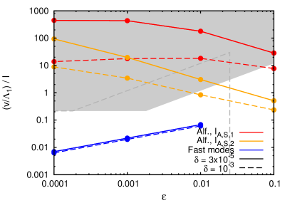
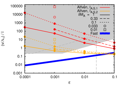
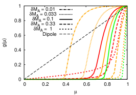
For a range of the parameters $\delta$ and $\delta\mathcal{M}_{\rm A}$, Fig. 1 plots $v/\left(\Lambda_{1}l\right)$ as a function of $\varepsilon$ for all six models listed in Table 1: A, B and E in the left panel, and C, D and F in the right panel. Models that fail to meet criterion (24) fall in the grey shaded region (for CRs of energy $1\,$PeV), or above the dashed grey line (for CRs of $100\,$TeV). In the latter case, the additional constraint $\varepsilon<0.025$ is included, which is an approximate implementation of the requirement that $r_{\rm L}<l$ also for CRs of several PeV. Model A is the most strongly affected by this criterion: out of the eight cases chosen, only $\{\varepsilon,\delta\}=\{10^{-1},10^{-3}\}$ is outside the shaded area. The fact that the observer is in the boundary layers (see Sect. 2.1) for such a large fraction of the parameter space is due to the fact that $\nu\ll 1$ over a large range of $\mu$. The CR mean free path $\lambda_{\parallel}$ is also quite large ($\lambda_{\parallel}/l$ versus $\varepsilon$ is plotted in Fig. 11 —left panel, in Appendix B), ranging from $\simeq 70\,l$ to $\simeq 2.0\times 10^{3}\,l$, substantially larger than the outer scale of the turbulence. In most cases, $\Lambda_{1}\lambda_{\parallel}/v\sim 10$, which implies that the distance between Earth and the boundaries of the flux tube must be $\approx{\rm a~{}few}\times\lambda_{\parallel}/10$ for criterion Eq. (11) to be satisfied.

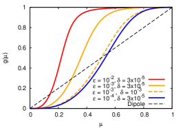
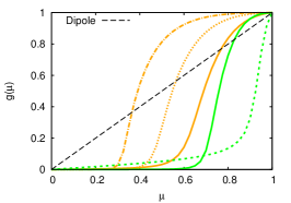
Our results on the anisotropy are presented in several ways. First, we quantify the ability of each model to give rise to a “hole” in the CR flux — which in our treatment can only occur axisymmetrically, i.e., around a direction parallel or antiparallel to the magnetic field — by plotting angular half-width, $\vartheta_{1/2}$, defined such that:

$$g\left(\cos\vartheta_{1/2}\right)=1/2\;.$$ (25)

Figure 2.— Half-width of the anisotropy, $\vartheta_{1/2}$, for GS turbulence and isotropic fast modes, using $R_{\rm n}=R_{\rm n,1}$ (upper row) or $R_{\rm n,2}$ (lower row). For a dipole anisotropy, $\vartheta_{1/2}=60^{\circ}$ (thin black dotted lines). Upper left panel: GS turbulence with $\mathcal{I}_{\rm A,S}=\mathcal{I}_{\rm A,S,1}$ (model A) and $\delta\in[10^{-8},10^{-1}]$ (see key), using the analytical formulae of Chandran (2000) for $D_{\mu\mu}$. Upper right panel and lower panels: $D_{\mu\mu}$ is calculated numerically. Red lines for GS turbulence with $\mathcal{I}_{\rm A,S,1}$ (models A and C), orange lines for $\mathcal{I}_{\rm A,S,2}$ (models B and D), and blue lines or areas for isotropic fast modes (models E and F). Filled circles correspond to calculations with parameter values outside the area shaded in grey, triangles correspond to those below the grey dashed line in Fig. 1. Otherwise, no symbols are plotted. Thick lines correspond to lines that are partially outside the shaded area in Fig. 1. Upper right panel: solid (dashed) lines for $\delta=3\times 10^{-5}$ ($\delta=10^{-3}$). Lower row: $\vartheta_{1/2}$ as a function of $\varepsilon$ (left), and as a function of $\delta\mathcal{M}_{\rm A}$ (right). See key in the lower left (resp. right) panel for the dependence of $\vartheta_{1/2}$ on $\delta\mathcal{M}_{\rm A}$ (resp. $\varepsilon$).

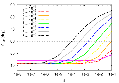
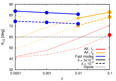
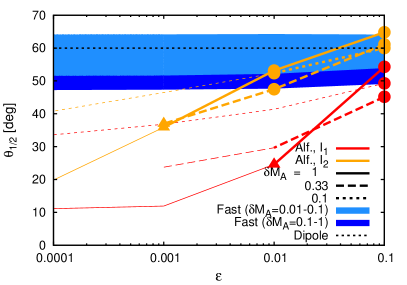
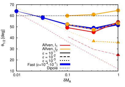
This quantity is plotted in Fig. 2. In the upper left panel, the analytic formulae given by Chandran (2000) for model A, are exploited to present the half-width as a function of $\varepsilon$ for a very wide range of $\delta$. The upper right panel (for models A, B and E) and lower left panel (for models C, D and F) also show $\vartheta_{1/2}$ as a function of $\varepsilon$, but for a more limited range of $\delta$ and $\delta\mathcal{M}_{\rm A}$. Finally, the lower right panel illustrates the functional dependence of $\vartheta_{1/2}$ on $\delta\mathcal{M}_{\rm A}$ for models C, D and F, for various values of $\varepsilon$. In each plot, we also show the result for a dipole anisotropy ($\vartheta_{1/2}=60^{\circ}$), and highlight those models that lie in the allowed region in Fig. 1.

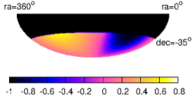
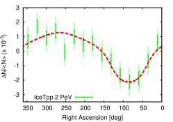
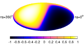
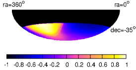
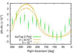
Each of the following seven figures presents panels containing details of the predicted anisotropy for the models in Table 1. Along with plots of the dimensionless scattering frequency $\nu(\mu)$ and the normalized anisotropy $g(\mu)$ against $\mu$, we also present 2D sky maps of the anisotropy and comparisons with the IceTop measurements. To construct these, we assume the interstellar magnetic field (which is measured with a precision of $\approx 20^{\circ}-30^{\circ}$) lies in the direction $(l_{\rm Gal}=47^{\circ},\,b_{\rm Gal}=25^{\circ})$, as given in Table 1 of Frisch et al. (2012). This choice leads to a minimum of the anisotropy at the same right ascension as that observed. A more sophisticated fit to the data would take into account the uncertainty in the magnetic field direction explicitly, see Sect. 4. At 400 TeV and 2 PeV median energy, IceTop provides the variation $\Delta N/\langle N\rangle$ of the CR flux as a function of right ascension, averaged over declinations between $-75^{\circ}$ and $-35^{\circ}$ (Aartsen et al., 2013). To compare these data with our predictions, we integrate our (axisymmetric) anisotropy over the range of phase and $\mu$ corresponding to IceTop’s range of declination, add a constant to ensure that the average over right ascension vanishes, and normalize the minimum value to coincide with the IceTop data.

3.1. Goldreich-Sridhar turbulence

Let us first consider incompressible Alfvénic turbulence with a GS power-spectrum.

3.1.1 Model A ($\mathcal{I}_{\rm A,S}=\mathcal{I}_{\rm A,S,1}$ and $R_{\rm n}=R_{\rm n,1}$)

Figure 3.— Model A, GS turbulence with $\mathcal{I}_{\rm A,S}=\mathcal{I}_{\rm A,S,1}$, and using $R_{\rm n,1}$. Upper left panel: $\nu$ as a function of $\mu$, for $\{\varepsilon,\delta\}=\{10^{-1},3\times 10^{-5}\}$ (thick red dotted line), $\{10^{-2},3\times 10^{-5}\}$ (black dotted), $\{10^{-3},3\times 10^{-5}\}$ (green dotted), $\{10^{-5},3\times 10^{-5}\}$ (black dashed-dotted), $\{10^{-1},10^{-2}\}$ (black solid), and $\{10^{-1},10^{-3}\}$ (thick red solid). Upper right panel: $g(\mu)$, using the same line types. Lower left and middle panels: $g(\mu)$ in equatorial coordinates for $\delta=3\times 10^{-5}$, and $\varepsilon=10^{-1}$ (left) or $\varepsilon=10^{-3}$ (middle). Lower right panel: relative CR intensity $\Delta N/\langle N\rangle$ at $-75^{\circ}\leq{\rm dec}\leq-35^{\circ}$, as a function of right ascension, compared with IceTop 2 PeV data set (Aartsen et al., 2013).

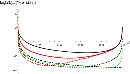
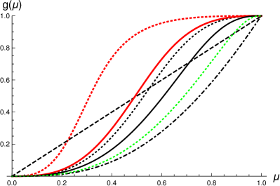
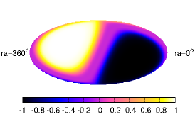
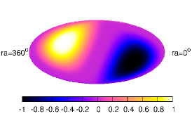
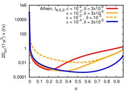
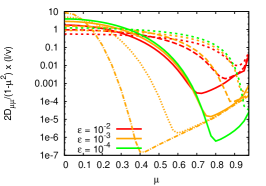
In Fig. 3, we plot $\nu$ and $g$ versus $\mu$ in the upper panels for $\delta=3\times 10^{-5}$, using red, black, and green dotted lines, for $\varepsilon=10^{-1}$, $\varepsilon=10^{-2}$, and $\varepsilon=10^{-3}$, respectively. The transition from the minimum of $\nu$ being located at small $\mu$ to it being located at $\mu\rightarrow 1$ corresponds to a transition in the shape of $g(\mu)$: it changes from a function with $\vartheta_{1/2}$ larger than for a dipole to a function with small cold spots $\vartheta_{1/2}\approx 40^{\circ}$. The value of $\mu$ where $\nu$ reaches its minimum is important, because it defines the region where $g^{\prime}(\mu)\propto 1/\nu$ reaches its maximum value. At any $\mu$ where $\nu$ is much greater than its minimum value, $g(\mu)$ looks flat. As can be seen in the upper right panel of Fig. 3, for the red dotted line (i.e. at large $\varepsilon=10^{-1}$) $g$ is close to 1 in a broad region $\mu\gtrsim 0.6$. If this case happens to be in a region of parameter space where the CR anisotropy is given by $g$ (i.e. Eq. (11) is satisfied), the anisotropy would consist of a large hot spot and a large cold spot, along the direction of magnetic field lines. When the CR energy decreases, the size of the hot and cold spots decreases, due to the aforementioned shift in of the minimum of $\nu$ to $\mu\rightarrow 1$ (see the black dotted and green dotted lines in the upper right panel). The black dashed-dotted line corresponds to an even lower CR energy, $\varepsilon=10^{-5}$, for the same $\delta$. $\vartheta_{1/2}$ is smaller than for $\varepsilon=10^{-3}$. We find that decreasing $\varepsilon$ to values smaller than $10^{-5}$ does not appreciably change the shape of $g$. Correspondingly, $\vartheta_{1/2}$ remains at its minimum in this region. In summary, the hot and cold spots become very wide and flat when $\varepsilon$ is large. The half width of the hot and cold spots reaches a minimum value of about $40^{\circ}$ when $\varepsilon$ is small. This behaviour of $\vartheta_{1/2}$ with $\varepsilon$ can be clearly seen in Fig. 2 (upper left panel), where we plot $\vartheta_{1/2}$ as a function of $\varepsilon$, for eight values of $\delta\in[10^{-1},10^{-8}]$. The larger $\delta$ is, the larger is the value of $\varepsilon$ above which $\vartheta_{1/2}$ significantly departs from its minimum value. At $\varepsilon$ fixed, increasing $\delta$ has qualitatively the same effect as decreasing $\varepsilon$ at $\delta$ fixed. The thick red solid (resp. black solid) line in the upper panels of Fig. 3 corresponds to $\delta=10^{-3}$ (resp. $\delta=10^{-2}$) and $\varepsilon=10^{-1}$. By comparing the red dashed, red solid, and black solid lines, one can see that $\vartheta_{1/2}$ decreases and tends towards the limiting behaviour found above for small $\varepsilon$.

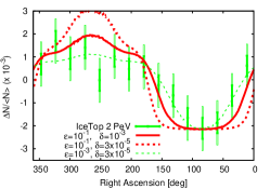
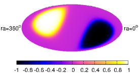
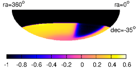
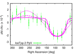
We now consider two rather “extreme” cases, $\{\varepsilon,\delta\}=\{10^{-1},3\times 10^{-5}\}$ and $\{10^{-3},3\times 10^{-5}\}$ and plot the corresponding anisotropy in equatorial coordinates in the lower left and centre panels of Fig. 3, respectively. In the first case, $\vartheta_{1/2}>60^{\circ}$, whereas in the second $\vartheta_{1/2}<60^{\circ}$, as can be seen in the upper right panel of Fig. 2. Both cases lie in the forbidden region of Fig. 1, i.e., the actual anisotropy at Earth is determined by the (unknown) boundary conditions at the ends of our flux tube, and not by $g$. Nevertheless, it is useful to study them, because they exhibit particularly clear features that are also present in the more realistic cases. In each panel, a large magenta region where $g$ is nearly constant and $\simeq 0$ is visible. It corresponds to directions on the sky that are almost perpendicular to the local field lines ($\mu\approx 0$). For a dipole, the magenta region would cover a much smaller area, and be barely visible with this color key. In the lower centre panel, the cold and hot spots are quite small. If the CR anisotropy were given by such a function, an experiment such as IceTop/IceCube, which observes part of the Southern hemisphere, would see only a single tight cold spot ($\simeq 40^{\circ}$ in size), surrounded by a region of approximately constant flux covering the rest of the visible sky. In the lower right panel of Fig. 3 we show the relative CR intensity $\Delta N/\langle N\rangle$ as a function of right ascension, at declinations $-75^{\circ}\leq{\rm dec}\leq-35^{\circ}$, as would be observed if the anisotropy were given by $g$, for three cases: $\{\varepsilon,\delta\}=\{10^{-1},3\times 10^{-5}\}$, $\{10^{-1},10^{-3}\}$, and $\{10^{-3},3\times 10^{-5}\}$. We keep the same line types and colors as in the two upper panels. Superimposed on this, we plot the 2 PeV data from IceTop (Aartsen et al., 2013) using green errorbars. For the case shown in the lower centre panel, the hot spot is almost completely out of sight in the Northern hemisphere: $\Delta N/\langle N\rangle$ displays a small cold spot and is rather flat elsewhere (see the thin green dotted line in the lower right panel). Although the model is ruled out by the criteria of Fig. 1, this line nevertheless provides a good fit to the 2 PeV data, whereas for both cases with $\varepsilon=10^{-1}$, the size of the cold spot is too large to fit the data. For $\varepsilon=10^{-1}$, $\delta=3\times 10^{-5}$, the half-width of the hot spot is so large that it would spill over into the Southern hemisphere and be visible to IceTop as a big bump in $\Delta N/\langle N\rangle$ at ${\rm RA}\approx 240^{\circ}-280^{\circ}$. This case is also ruled out by Fig. 1.

In summary, there is not enough freedom to permit $v/\Lambda_{1}$ to be sufficiently small, whilst, at the same time, keeping $\vartheta_{1/2}$ small. Indeed, $\varepsilon$ cannot be increased to values much larger than $10^{-1}$ because the CR gyroradius should remain smaller than the outer scale of the turbulence. Also, $\delta$ cannot be increased further: $\delta=10^{-3}$ already corresponds to a rather large value of $v_{\rm A}\simeq 300$ km s^-1, compared to that expected in our local interstellar medium. We show with red lines in Fig. 2 (upper right panel) the values of $\vartheta_{1/2}$ for these 8 cases. The red dot corresponds to the only case outside the shaded area in Fig. 1. Its $\vartheta_{1/2}$ is close to $60^{\circ}$. However, $v/\Lambda_{1}$ is strongly dependent on $\mathcal{I}_{\rm A,S}$, and may be substantially smaller, see below.

3.1.2 Model B ($\mathcal{I}_{\rm A,S}=\mathcal{I}_{\rm A,S,2}$ and $R_{\rm n}=R_{\rm n,1}$)

Figure 4.— Model B, GS turbulence with $\mathcal{I}_{\rm A,S}=\mathcal{I}_{\rm A,S,2}$, and using $R_{\rm n,1}$. Upper middle panel: $\nu$ as a function of $\mu$, for $\{\varepsilon,\delta\}=\{10^{-1},3\times 10^{-5}\}$, $\{10^{-1},10^{-3}\}$, $\{10^{-2},10^{-3}\}$, and $\{10^{-4},10^{-3}\}$ — see key. (The same line types are used in the upper right and lower right panels). Upper right panel: $g$ as a function of $\mu$. Lower left panel: anisotropy $g(\mu)$ in equatorial coordinates, for $\{10^{-2},10^{-3}\}$. Lower middle panel: predicted CR anisotropy, with extremum amplitude renormalized to $\pm 1$, in the field of view of IceTop, for $\{10^{-2},10^{-3}\}$. The anisotropy is calculated here with respect to the averaged flux in each declination band. Lower right panel: relative CR intensity $\Delta N/\langle N\rangle$ at $-75^{\circ}\leq{\rm dec}\leq-35^{\circ}$, as a function of right ascension, and compared with IceTop 2 PeV data (Aartsen et al., 2013). Upper left panel: comparison of the contributions from Alfvén modes (orange lines) and pseudo-Alfvén modes (blue lines) to $\nu$, for GS turbulence with $\mathcal{I}_{\rm A,S}=\mathcal{I}_{\rm A,S,2}$ (solid lines) and with $\mathcal{I}_{\rm A,S,1}$ (dashed lines), both for $R_{\rm n}=R_{\rm n,1}$ (models A & B) and $\{\varepsilon,\delta\}=\{10^{-3},10^{-3}\}$.

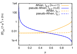
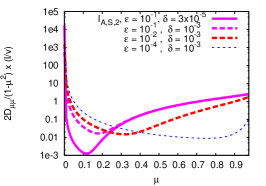
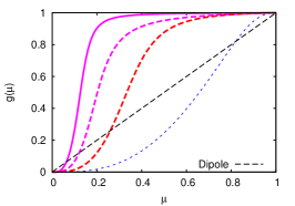
We now consider GS turbulence with a more gradual (exponential) form of anisotropy $\mathcal{I}_{\rm A,S}=\mathcal{I}_{\rm A,S,2}$ (model B) and calculate $D_{\mu\mu}$ numerically (see Eqs. (A3) and (A4)) for eight cases: $\varepsilon=10^{-1},10^{-2},10^{-3},10^{-4}$, with $\delta=3\times 10^{-5}$ and $\delta=10^{-3}$. As can be seen in Fig. 1 and Fig. 11 (left panels), this model more easily satisfies the constraint on $\Lambda_{1}$, signalling an increased CR scattering rate. This arises from a larger contribution to $\nu$ by Alfvén modes at medium and large values of $|\mu|$. In Fig. 4 (upper left panel), we compare the contributions from Alfvén (orange lines) and pseudo-Alfvén (blue lines) modes to $\nu$, in models A (dashed lines) and B (solid lines), using $\{\varepsilon,\delta\}=\{10^{-3},10^{-3}\}$. The blue dashed and blue solid lines are nearly coincident, i.e., the contribution from pseudo-Alfvén modes is the same in each model. In contrast, the contribution from Alfvén modes in model B is larger by up to two orders of magnitude, in the range $0.5\lesssim\mu\leq 1$. Therefore, taking an exponential cutoff in $k_{\parallel}$ instead of a step function makes a significant difference for CR scattering off Alfvén waves; the small but finite power present in modes with “large” $k_{\parallel}$, when an exponential cutoff is used instead of a sharp Heaviside function has a marked impact.

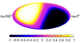
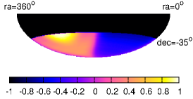
According to Fig. 1 (left panel), three out of the eight cases calculated for model B are outside the shaded area: $\{\varepsilon,\delta\}=\{10^{-1},3\times 10^{-5}\}$, $\{10^{-1},10^{-3}\}$, and $\{10^{-2},10^{-3}\}$. We plot $\nu$ and $g(\mu)$ in the upper centre and upper right panels of Fig. 4, using thick magenta solid lines, thick magenta dashed lines, and thick red dashed lines, for $\{10^{-1},3\times 10^{-5}\}$, $\{10^{-1},10^{-3}\}$, and $\{10^{-2},10^{-3}\}$, respectively. The scattering frequency $\nu$ has a large peak at $\mu=0$, followed by a minimum in the range $\mu=0.1-0.3$, after which it recovers at larger $\mu$. This leads to an anisotropy $g(\mu)$ that is rather flat in a small range of $\mu\lesssim 0.1$, and then rapidly increases towards unity. As can be seen in Fig. 2 (upper right panel), the size of the hot (and cold) spot is quite large for these three cases (indicated by large orange dots in the upper right panel), even larger than for model A (red lines) at the same value of $\varepsilon$ and for the dipole anisotropy. We calculate in Fig. 4 (lower right panel) the resulting $\Delta N/\langle N\rangle$ as a function of right ascension, at $-75^{\circ}\leq{\rm dec}\leq-35^{\circ}$, and compare it with IceTop 2 PeV data. The cold spot size and shape are incompatible with the data, as is also the presence of a large maximum around RA $\approx 250^{\circ}$. Sky maps for the anisotropy in the “least bad” case, $\{10^{-2},10^{-3}\}$, are shown in the lower left and lower centre panels of Fig. 4: full sky (left) and Southern sky in the field of view of IceTop (centre). Model B is clearly ruled out by the data.

We point out that, although the size of the cold spot decreases with $\varepsilon$ (see the orange lines in the upper right panel of Fig. 2), all cases with $\vartheta_{1/2}<60^{\circ}$ are located well inside the forbidden region shaded in grey in Fig. 1. For cases inside this region, we use thinner lines and do not show results with large dots in Fig 2. The orange triangle in this figure corresponds to the case that lies both inside the shaded region and below the grey dashed line in Fig. 1. In the upper centre, upper right, and lower right panels of Fig. 4, we plot the case $\{10^{-4},10^{-3}\}$ with thin blue dotted lines. Here again, the cold spot is small enough to fit the 2 PeV data, but only where the anisotropy is not given by $g$, i.e., in where condition (11) is not satisfied.

3.1.3 Model C ($\mathcal{I}_{\rm A,S}=\mathcal{I}_{\rm A,S,1}$ and $R_{\rm n}=R_{\rm n,2}$)

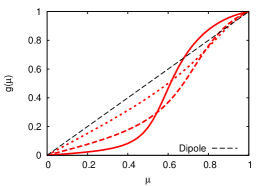
We now turn to the broad resonance function, $R_{\rm n,2}$, and start with $\mathcal{I}_{\rm A,S,1}$ (model C). We calculate $D_{\mu\mu}$ from Eqs. (A6) and (A7), for 13 combinations of $\varepsilon\in\{10^{-1},10^{-2},10^{-3},10^{-4}\}$ and $\delta\mathcal{M}_{\rm A}\in\{1,0.33,0.1,0.033,0.01\}$ (see the red symbols in the right panel of Fig. 1).

Figure 5.— Model C, GS turbulence with $\mathcal{I}_{\rm A,S}=\mathcal{I}_{\rm A,S,1}$, and using $R_{\rm n,2}$. $\varepsilon=10^{-1}$ in all panels, except in the upper left one. Upper middle panel: $\nu$ as a function of $\mu$, for $\delta\mathcal{M}_{\rm A}\in\{0.1,0.33,1\}$, see key. (Same line types used in the upper right and lower right panels.) Upper right panel: $g$ as a function of $\mu$. Lower left panel: anisotropy $g(\mu)$ in equatorial coordinates, for $\delta\mathcal{M}_{\rm A}=0.1$. Lower middle panel: predicted CR anisotropy, with extremum amplitude renormalized to $\pm 1$, in the field of view of IceTop, for $\delta\mathcal{M}_{\rm A}=0.1$. The anisotropy is calculated here with respect to the averaged flux in each declination band. Lower right panel: relative CR intensity $\Delta N/\langle N\rangle$ at $-75^{\circ}\leq{\rm dec}\leq-35^{\circ}$, as a function of right ascension, and compared with IceTop 2 PeV data (Aartsen et al., 2013). Upper left panel: comparison of the contributions from Alfvén modes (orange lines for $n=\pm 1$) and pseudo-Alfvén modes (blue lines for $n=0$, and magenta lines for $n=\pm 1$) to $\nu$, for GS turbulence with $\mathcal{I}_{\rm A,S}=\mathcal{I}_{\rm A,S,1}$ (dashed lines) and with $\mathcal{I}_{\rm A,S,2}$ (solid lines), both for $R_{\rm n}=R_{\rm n,2}$ (models C & D) and $\{\varepsilon,\delta\mathcal{M}_{\rm A}\}=\{10^{-3},0.1\}$.

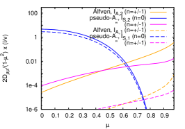
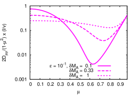
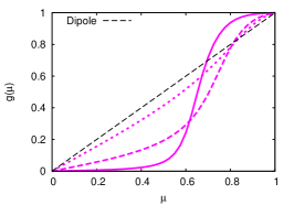
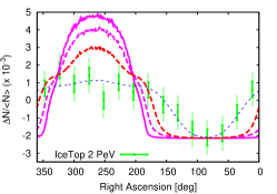
In Fig. 5 (upper left panel), we plot the contribution to the scattering frequency $\nu$ of the $n=0$ term for pseudo-Alfvén waves using a blue, dashed line, and that of the $n=\pm 1$ terms for Alfvén waves using an orange dashed line (the solid lines will be explained in the next subsection). The magenta dashed line corresponds to the $n=\pm 1$ contribution from pseudo-Alfvén modes (Eq. (A8)), which is found to be subdominant at all $\mu$ when $\delta\mathcal{M}_{\rm A}\gtrsim 0.1$. As in model A, scattering around $\mu=0$ is predominantly provided by pseudo-Alfvén waves, and scattering at large $|\mu|$ is dominated by scattering off Alfvén waves. The height of the peak at $\mu=0$ is smaller, but this is of little relevance for the shape of the CR anisotropy. A more important difference between the broad and narrow resonance functions $R_{\rm n,1}$ (A) and $R_{\rm n,2}$ (C) is that the width of the peak is larger in the latter, unless $\delta\mathcal{M}_{\rm A}\ll 0.01$. This has the important consequences of both reducing the size of the hot/cold spots and reducing $v/\Lambda_{1}$, as can be seen in Figs. 1 and 2.

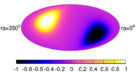
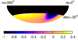
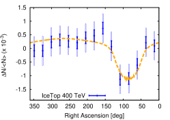
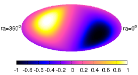
Out of the 13 cases, three are in the allowed, non-shaded area of Fig. 1: $\varepsilon=10^{-1}$ with $\delta\mathcal{M}_{\rm A}=1,0.33,0.1$. In the upper centre, upper right, and lower right panels of Fig. 5, we plot, for these three cases, $\nu(\mu)$, $g(\mu)$, and $\Delta N/\langle N\rangle$ (see the line types in the key of the upper centre panel). With $\delta\mathcal{M}_{\rm A}=1$ (dotted magenta line), the contribution from pseudo-Alfvén modes around $\mu=0$ is so wide that $\nu$ is rather flat on $0\leq\mu\leq 1$. The corresponding anisotropy is then not far from being a dipole — see the upper right panel, and it does not fit the small cold spot in IceTop data — see the lower right panel. On the other hand, both $\delta\mathcal{M}_{\rm A}=0.1$ and $\delta\mathcal{M}_{\rm A}=0.33$ provide a good fit to the 2 PeV data: they have a moderately low minimum in $\nu$ at sufficiently large values of $\mu\simeq 0.6-0.75$ (see upper centre panel), around the transition from scattering off pseudo-Alfvén modes to scattering off Alfvén modes. This leads to a rather flat $g$ at $\mu\lesssim 0.5$–$0.6$, and to smaller hot and cold spots around $\mu=\pm 1$, in good agreement with the IceTop 2 PeV data (see the solid and dashed magenta lines in the lower right panel). We show in the lower left and centre panels the full-sky anisotropy (left) and the anisotropy in the field of view of IceTop (middle) for one of these two good cases, $\{\varepsilon,\delta\mathcal{M}_{\rm A}\}=\{10^{-1},0.1\}$. The presence of a flat CR flux in a broad region in $\mu$ outside the cold and hot spots is visible in both panels. This conceals the hot spot in the Northern hemisphere, while providing a rather flat CR flux outside a tight cold spot, see the lower middle panel.

In the lower panels of Fig. 2, $\vartheta_{1/2}$ is plotted with red lines, as a function of $\varepsilon$ (left), and as a function of $\delta\mathcal{M}_{\rm A}$ (right). Although a good fit to the 2 PeV data, the values of $\vartheta_{1/2}\approx 45^{\circ}-50^{\circ}$ at $\varepsilon=10^{-1}$ are not small enough to account for the smaller cold spot in the 400 TeV data. Decreasing $\varepsilon$ causes $\vartheta_{1/2}$ to drop to values much lower than $40^{\circ}$. As a result, $\{10^{-2},1\}$ is the only point with $\varepsilon<10^{-1}$ that satisfies Eq. (11) for 100 TeV, i.e., which is below the grey dashed line in Fig. 1 (right panel), whilst, at the same time providing an acceptable fit to the 400 TeV data. However, $\varepsilon=10^{-1}$, $\delta\mathcal{M}_{\rm A}=1$ does not provide a good fit to the higher-energy data set.

3.1.4 Model D ($\mathcal{I}_{\rm A,S}=\mathcal{I}_{\rm A,S,2}$ and $R_{\rm n}=R_{\rm n,2}$)

Figure 6.— Model D, GS turbulence with $\mathcal{I}_{\rm A,S}=\mathcal{I}_{\rm A,S,2}$, and using $R_{\rm n,2}$: $\nu(\mu)$ (left column), $g(\mu)$ (middle column), and relative CR intensity $\Delta N/\langle N\rangle$ in the declination band $-75^{\circ}$ to $-35^{\circ}$, as a function of right ascension, and compared with IceTop 2 PeV or 400 TeV data sets from Aartsen et al. (2013) (right column). Upper row: $\varepsilon=10^{-1}$; Middle row: $\varepsilon=10^{-2}$; Lower row: $\varepsilon=10^{-3}$. Each line type corresponds to a different value of $\delta\mathcal{M}_{\rm A}\in\{0.1,0.33,1\}$. Identical line types in each row, see keys in the left panels.

Figure 7.— Large-scale CR anisotropy for model D, GS turbulence with $\mathcal{I}_{\rm A,S}=\mathcal{I}_{\rm A,S,2}$, and using $R_{\rm n,2}$ with $\delta\mathcal{M}_{\rm A}=0.33$. Upper row: $\varepsilon=10^{-3}$. Lower row: $\varepsilon=10^{-2}$, i.e. the CR energy is 10 times larger than in the upper row. Left column: anisotropy $g(\mu)$ in equatorial coordinates. Middle column: predicted CR anisotropy, with extremum amplitude renormalized to $\pm 1$, in the field of view of IceTop. The anisotropy is calculated here with respect to the averaged flux in each declination band. Right column: relative CR intensity $\Delta N/\langle N\rangle$ at $-75^{\circ}\leq{\rm dec}\leq-35^{\circ}$, as a function of right ascension, compared with IceTop data (Aartsen et al., 2013) at 400 TeV (upper row) and 2 PeV (lower row).

We now calculate $D_{\mu\mu}$, using Eqs. (A9) and (A10), for the same 13 combinations of $\varepsilon$ and $\delta\mathcal{M}_{\rm A}$ as in Sect. 3.1.3.

In the upper left panel of Fig. 5, we plot for $\{\varepsilon,\delta\mathcal{M}_{\rm A}\}=\{10^{-3},0.1\}$ the $n=\pm 1$ contribution to $\nu$ from Alfvén modes and the $n=0$ contribution from pseudo-Alfvén modes using orange and blue solid lines, respectively. We also show the $n=\pm 1$ contribution from pseudo-Alfvén modes (Eq. (A11)) using a magenta solid line. At $\delta\mathcal{M}_{\rm A}\geq 0.1$, the magenta line is below the orange and blue solid lines at all $\mu$, as was also found for model C. At $\delta\mathcal{M}_{\rm A}=0.01,0.033$, the $n=\pm 1$ contribution from pseudo-Alfvén modes dominates in only a small range of $\mu$, and its impact on $g$ is weak. By comparing the solid orange and blue lines to the dashed orange and blue ones, we note that using $\mathcal{I}_{\rm A,S,2}$ (model D) instead of $\mathcal{I}_{\rm A,S,1}$ (model C) again strongly increases the CR scattering off Alfvén waves, as was the case with the narrow resonance function $R_{\rm n,1}$ (models A and B): at all $\mu$, the solid orange line is two to three orders of magnitude above the dashed orange one. Scattering off pseudo-Alfvén waves is only slightly increased by this change (see the blue lines).

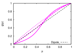
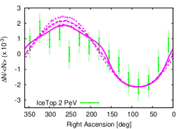
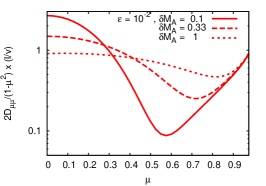
This increased scattering is manifested in Fig. 1 (right panel) by a reduction in $v/\Lambda_{1}$ of one to four orders of magnitude, so that larger portions of the orange lines and six out of the computed 13 cases are in the permitted region: $\varepsilon=10^{-1}$ or $10^{-2}$, with $\delta\mathcal{M}_{\rm A}=1,\,0.33$ or 0.1. Two cases, namely $\varepsilon=10^{-3}$ with $\delta\mathcal{M}_{\rm A}=0.33$ or 1, are in the allowed region for 100 TeV CR (see the grey dashed line in Fig.1), and thence can be compared with the 400 TeV data set. The allowed region for 400 TeV CRs is somewhat smaller than for 100 TeV CRs. However, it is still interesting to consider these two points at $\varepsilon=10^{-3}$, because our coarse resolution in $\varepsilon$ (one point per decade) does not allow us to test more favourable points at larger $\varepsilon$ (e.g. $\varepsilon=2\times 10^{-3}$), on the same lines with $\delta\mathcal{M}_{\rm A}=0.33$ or 1.

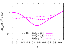
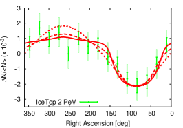
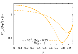
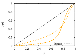
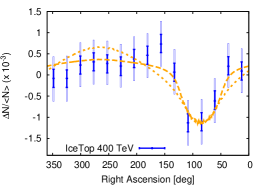
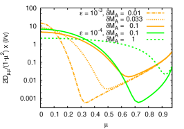
In Fig. 6, we plot for these eight cases: $\nu$ (left column), $g$ (centre column), and $\Delta N/\langle N\rangle$ compared with IceTop 2 PeV or 400 TeV data (right column). Each $\delta\mathcal{M}_{\rm A}$ has its own line type, see keys in the left column plots. In the first row, $\varepsilon=10^{-1}$: for $\delta\mathcal{M}_{\rm A}=1$ and 0.33, the scattering rate is about the same at all $\mu$ (left), and the anisotropy is close to a dipole (centre). The case $\delta\mathcal{M}_{\rm A}=0.1$ is also close to a dipole, so that none of these three cases fits IceTop data (see the three orange dots on the orange solid line in Fig. 2, lower right panel). For smaller $\varepsilon$, $\vartheta_{1/2}$ decreases significantly: in the second row of Fig. 6, $\varepsilon=10^{-2}$, and both $\delta\mathcal{M}_{\rm A}=0.33$ and 0.1 fit the IceTop 2 PeV data. On the other hand, $\delta\mathcal{M}_{\rm A}=1$ remains close to being a dipole. In the third row, $\varepsilon=10^{-3}$, and the case $\delta\mathcal{M}_{\rm A}=0.33$ provides a sufficiently small cold spot to fit the 400 TeV data reasonably well. For $\delta\mathcal{M}_{\rm A}=1$, the predicted cold spot is too wide.

In Fig. 7, we study the dependence of the anisotropy on CR energy for a fixed set of parameters of the turbulence and resonance function. We set $\delta\mathcal{M}_{\rm A}$ to $0.33$. Since $l$ is fixed, a ten-fold increase in CR energy corresponds to a ten-fold increase of $\varepsilon$. Accordingly, we set $\varepsilon=10^{-3}$ in the upper row, and $\varepsilon=10^{-2}$ in the lower row. The left column contains all-sky plots of $g(\mu)$, the centre column the anisotropy within IceTop field of view at ${\rm dec}\leq-35^{\circ}$, and the right column, $\Delta N/\langle N\rangle$. The IceTop data, and their energy-dependence are well reproduced for these values of $\varepsilon$ and the turbulence parameters: at $\varepsilon=10^{-3}$, the 400 TeV data fits well both the small cold spot and the large flatter region. On increasing the CR energy by a factor of 10 (close to the nominal factor five difference between the “400 TeV” and “2 PeV” data sets) the size of the cold spot increases and the higher-energy data is then also well fitted (see lower row).

Calculations of $\nu$ and $g$ for all cases located in the shaded areas in Figure 1, which were not presented in Sections 3.1.2–3.1.4, can be found in Appendix C, Figure 12.

3.2. Fast magnetosonic modes

We now treat the case in which the turbulent fluctuations are dominated by fast magnetosonic waves, which have an isotropic spectrum with intensity $\propto k^{-3/2}$.

3.2.1 Model E ($R_{\rm n}=R_{\rm n,1}$)

Figure 8.— Model E, isotropic fast modes, using $R_{\rm n,1}$. Upper left panel: $\nu$ as a function of $\mu$. Red lines for $\varepsilon=10^{-2}$, orange for $\varepsilon=10^{-3}$, and green for $\varepsilon=10^{-4}$. Solid (dashed) lines for $\delta=3\times 10^{-5}$ ($\delta=10^{-3}$). Upper right panel: $g$ versus $\mu$. Lower left panel: anisotropy $g(\mu)$ in equatorial coordinates, for $\delta=3\times 10^{-5}$ (and $\varepsilon=10^{-3}$). Lower middle panel: predicted CR anisotropy, with extremum amplitude renormalized to $\pm 1$, in the field of view of IceTop. Same values of $\varepsilon$ and $\delta$. The anisotropy is calculated here with respect to the averaged flux in each declination band. Lower right panel: relative CR intensity $\Delta N/\langle N\rangle$ at $-75^{\circ}\leq{\rm dec}\leq-35^{\circ}$, as a function of right ascension, and compared with IceTop 2 PeV data (Aartsen et al., 2013). $\delta\in\{3\times 10^{-5},10^{-3}\}$, see key.

Using the narrow resonance function $R_{n,1}$, we calculate numerically the $n=0,\pm 1$ contributions of fast modes to $D_{\mu\mu}$ – see Eqs. (A12) and (A13), for 6 cases: $\varepsilon\in\{10^{-2},10^{-3},10^{-4}\}$, with $\delta=3\times 10^{-5}$ or $10^{-3}$.

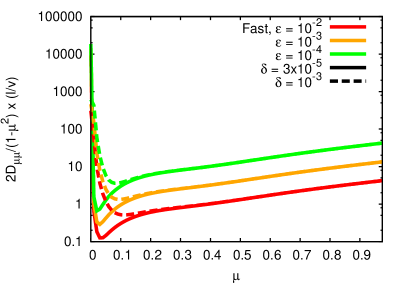
The scattering rate $\nu$ is shown in Fig. 8 (upper left panel). There is a large, narrow peak at $\mu=0$, as in the previous models of GS turbulence (A and B) with this resonance function, which is due here to the $n=0$ contribution from fast modes. As in GS turbulence, the peak broadens when $\delta$ is increased, as can be seen by comparing the solid and dashed lines in the upper left panel. The minimum is located at the value of $|\mu|$ above which the $n=\pm 1$ term starts to dominate over the $n=0$ term. An important difference compared to the corresponding models of GS turbulence is that the $n=\pm 1$ contribution of fast modes is typically a few orders of magnitude larger than that of the Alfvén modes of GS turbulence, leading to values of $v/\Lambda_{1}$ that are about two to four orders of magnitude smaller than those for GS turbulence, as shown in the left panel of Fig. 1, where we plot $(v/\Lambda_{1})/l$ versus $\varepsilon$ with blue lines. For all the parameters chosen, this quantity lies in the permitted region, outside the shaded area. The shape of the function $\nu(\mu)$ does not change significantly with energy (Fig. 8, upper left panel). Its absolute value is larger for smaller $\varepsilon$, as expected. Consequently, $g(\mu)$ also does not change significantly with energy within the energy range studied. We plot $g$ in the upper right panel: both lines, for $\delta=3\times 10^{-5}$ and $\delta=10^{-3}$, are well above the black dashed line for a dipole. This implies that the hot and cold spots are much wider than those for a dipole, see also the blue lines in upper right panel of Fig. 2. This is in clear contradiction with existing observations. We plot in the lower row of Fig. 8 a full-sky map for $\delta=3\times 10^{-5}$ (left panel), the anisotropy within IceTop field of view for the same value of $\delta$ (centre), and a comparison of $\Delta N/\langle N\rangle$ with IceTop 2 PeV data for both values of $\delta$ (right). These maps show no resemblance to the observed anisotropy, which rules out this model.

3.2.2 Model F ($R_{\rm n}=R_{\rm n,2}$)

Figure 9.— Model F, isotropic fast modes, using $R_{\rm n,2}$. $\varepsilon=10^{-3}$ in all panels, and each line type corresponds to a different value of $\delta\mathcal{M}_{\rm A}\in\{0.01,0.033,0.1,0.33,1\}$, see keys. Upper left panel: $\nu$ as a function of $\mu$. Upper middle panel: $g$ as a function of $\mu$. Upper right panel: relative CR intensity $\Delta N/\langle N\rangle$ at $-75^{\circ}\leq{\rm dec}\leq-35^{\circ}$, as a function of right ascension, and compared with IceTop 2 PeV data (Aartsen et al., 2013) for $\delta\mathcal{M}_{\rm A}\in\{0.01,0.033,1\}$. Lower left panel: predicted CR anisotropy, with extremum amplitude renormalized to $\pm 1$, in the field of view of IceTop for $\delta\mathcal{M}_{\rm A}=0.1$. The anisotropy is calculated here with respect to the averaged flux in each declination band. Lower middle and lower right panels: $\Delta N/\langle N\rangle$ for $\delta\mathcal{M}_{\rm A}\in\{0.1,0.33\}$, compared with IceTop 2 PeV (middle) and 400 TeV (right) data.

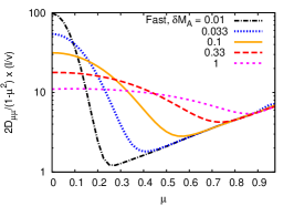
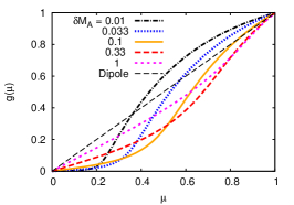
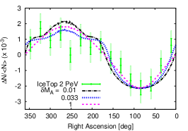
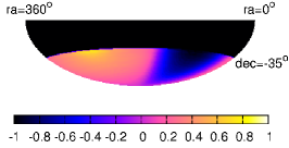
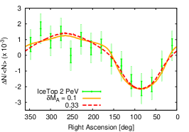
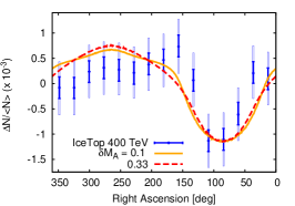
Taking now the broad resonance function, $R_{n,2}$, we calculate numerically the $n=0,\pm 1$ contributions of fast modes to $D_{\mu\mu}$ –see Eqs. (A14) and (A15), for 20 combinations of $\varepsilon$ and $\delta$: $\varepsilon\in\{10^{-1},10^{-2},10^{-3},10^{-4}\}$, $\delta\mathcal{M}_{\rm A}\in\{1,0.33,0.1,0.033,0.01\}$. In Fig. 1, $(v/\Lambda_{1})/l$ is shown as a function of $\varepsilon$ as a broad, blue band in the right panel, which illustrates the range of values we find for $0.01\leq\delta\mathcal{M}_{\rm A}\leq 1$. All values of $(v/\Lambda_{1})/l$ are outside the area shaded in grey, and, therefore, viable in the sense that the boundary layers of the flux tube are thin, so that the observed anisotropy should correspond to the predicted one.

In this energy range, we find no noticeable dependence of $g(\mu)$ on $\varepsilon$. Results for $\nu$ are presented at $\varepsilon=10^{-3}$, as an example. We plot in Fig. 9 (upper left panel) $\nu$ versus $\mu$ for all five tested values of $\delta\mathcal{M}_{\rm A}$. As in Sect. 3.2.1, the minimum corresponds to the separation between the low-$\mu$ region, where the $n=0$ term dominates, and the high-$\mu$ region, where the $n=\pm 1$ term dominates. The width of the peak around $\mu=0$ increases with increasing $\delta\mathcal{M}_{\rm A}$. This is reminiscent of the behaviour of the contribution of pseudo-Alfvén modes in GS turbulence (models C and D). Results for $g(\mu)$ are shown in the upper centre panel. The size of the hot/cold spot decreases with increasing $\delta\mathcal{M}_{\rm A}$ in the range $0.01-0.33$, but at $\delta\mathcal{M}_{\rm A}=1$, where $\nu$ is almost independent of $\mu$, the anisotropy moves closer to the result for a dipole — see the magenta dotted line and red dashed line in the upper centre panel. This behaviour with $\delta\mathcal{M}_{\rm A}$ is also visible in the lower right panel of Fig. 2. The minimum $\vartheta_{1/2}$ ($\simeq 47^{\circ}$) is reached at $\delta\mathcal{M}_{\rm A}=0.33$, although the value of $\vartheta_{1/2}$ at $\delta\mathcal{M}_{\rm A}=0.1$ is not much larger. We plot our predictions for $\Delta N/\langle N\rangle$ and compare them with the 2 PeV data set in the upper right and lower centre panels of Fig. 9. The cold spot is too large for $\delta\mathcal{M}_{\rm A}=0.01$, $0.033$, and $1$. On the other hand, $\delta\mathcal{M}_{\rm A}=0.1$ and $\delta\mathcal{M}_{\rm A}=0.33$ provide a satisfactory fit to the data. Although $\vartheta_{1/2}$ is slightly smaller for 0.33 than for 0.1, the shape of the anisotropy appears to be slightly better at $\delta\mathcal{M}_{\rm A}=0.1$ — in the latter case, $\Delta N/\langle N\rangle$ is flatter in the region around $160^{\circ}\leq{\rm RA}\leq 360^{\circ}$, see lower centre panel. In the lower left panel, we plot a sky map for $\delta\mathcal{M}_{\rm A}=0.1$, as would be observed within the field of view of IceTop, at ${\rm dec}\leq-35^{\circ}$. The qualitative agreement with the IceTop sky map at 2 PeV is good. However, none of the values of $\delta\mathcal{M}_{\rm A}\in[0.01,1]$ provide an acceptable fit to the smaller cold spot in the 400 TeV data. We show this in the lower right panel which compares the two cases with the smallest cold spots ($\delta\mathcal{M}_{\rm A}=0.1$ and 0.33) to IceTop 400 TeV data set. If such a small cold spot at 400 TeV were to be confirmed in the future, this could have important implications, as we discuss below.

4. Discussion and perspectives

The model developed in Sect. 2 assumes that CRs propagate in magnetic turbulence with a strong background field. Our approach requires the CR Larmor radius and mean free path to remain smaller than the coherence length of the interstellar magnetic field. We enforce these conditions by keeping $\varepsilon\ll 1$, and restricting our study to the non-shaded area of Fig. 1. Also, we take the anisotropy to be parallel to the regular field. In a 3D model, the perpendicular component of the CR density gradient would give rise to a perpendicular component in the anisotropy, but we neglect it here, in line with the observations of Schwadron et al. (2014). We further assume the turbulence to be homogeneous, i.e. to have properties that do not vary significantly within the $\sim 10$ pc flux tube in which we solve Eq. (1). In general, the coefficient $D_{\mu\mu}$ could vary within the flux tube, and the pitch-angle scattering rate could also depend on the gyrophase. However, these effects would make the problem intractable analytically. Finally, we note that imbalanced turbulence would lead to an asymmetry in the large-scale anisotropy within our model. Such an asymmetry is absent from the examples we have chosen to test in this paper, but it would be straightforward to include it.

Within the confines of this simplified model, the results of the previous section demonstrate explicitly that the large-scale anisotropy can take on a variety of forms, depending on the turbulence model and its parameters. In some cases (e.g., models C, D and F from Table 1, with an unrealistically large $\delta\mathcal{M}_{\rm A}=1$), this can resemble a simple dipole anisotropy. However, this is not the generic form and is also not predicted for any reasonable scenario, including that of isotropic fast-mode turbulence. In fact, only the physically unfounded assumption of isotropic pitch-angle scattering, $D_{\mu\mu}\propto 1-\mu^{2}$, leads to a pure dipole anisotropy. It is, therefore, not only unsurprising, but also reassuring that measurements of the large-scale anisotropy (e.g., Aartsen et al., 2013) cannot be reconciled with a pure dipole anisotropy.

A generic feature of the models we study is that the scattering frequency $\nu$ has a peak around $\mu=0$. This corresponds to the “transit-time damping” mentioned, for example, by Yan & Lazarian (2008). We argue that this leads to a flattening of the large-scale CR anisotropy in directions approximately perpendicular to the local magnetic field, which is compatible with IceCube (Abbasi et al., 2012) and IceTop (Aartsen et al., 2013) data at energies $\gtrsim 100$ TeV. This feature may also exist in the low-energy ($\sim 10$ TeV) data of IceCube, see Fig. 9 in Aartsen et al. (2016): the measured relative intensity is rather flat on ${\rm RA}\approx 0^{\circ}-100^{\circ}$, i.e. in the direction opposite to the minimum at ${\rm RA}\approx 200^{\circ}-250^{\circ}$. It is worth noting that such a feature naturally appears in all cases of turbulence we studied, without any fine-tuning of the theory. In the case of GS turbulence, the peak of $\nu$ around $\mu=0$ is due to pseudo-Alfvén waves. In the case of compressible turbulence, the peak is due to the $n=0$ term for fast modes in Eq. (20). In physical terms, this flattening can be understood as follows. In Eq. (12), the CR density is $\propto x$. If $\nu$ is large on $-\Delta\mu\leq\mu\leq+\Delta\mu$, the “last scattering surface” for CRs arriving from these directions is relatively close to Earth. Thence, they come from closeby regions of the local interstellar medium with small $x$ values, where the CR densities and distribution functions are similar. This leads to an anisotropy, $g$, that is approximately constant on $-\Delta\mu\leq\mu\leq+\Delta\mu$.

The peak at $\mu\approx 0$ may appear either narrow or broad depending on the type of resonance function and on the level of scattering at larger values of $|\mu|$. The dominant contribution to CR scattering at large $|\mu|$ is shear Alfvén modes for GS turbulence, and the $n=\pm 1$ term for fast modes. The minimum in $\nu$ occurs around the value of $\mu$ where the dominant contribution to scattering changes.

An important difference between the two resonance functions we used is that $R_{\rm n,2}$ tends to produce broader peaks around $\mu=0$ than $R_{\rm n,1}$, unless $\delta\mathcal{M}_{\rm A}$ is very small ($\ll 0.01$). As a consequence, the half-width of the anisotropy, which characterises the size of the spots at $\mu=\pm 1$, is usually smaller for $R_{\rm n,2}$ than for $R_{\rm n,1}$. We note that this is not systematically the case: for example, when the contribution to $\nu$ from shear Alfvén waves at large $|\mu|$ is at about the same level as the contribution from pseudo-Alfvén waves at smaller $|\mu|$, the anisotropy tends towards a dipole and $\vartheta_{1/2}\rightarrow 60^{\circ}$, see, for example, model D for GS turbulence with $\mathcal{I}_{\rm A,S}=\mathcal{I}_{\rm A,S,2}$, $R_{\rm n}=R_{\rm n,2}$, $\varepsilon=10^{-1}$, and $\delta\mathcal{M}_{\rm A}=1$ in Fig. 6 (upper row). Nonetheless, in most tested cases that lie in the allowed region in Fig. 1, i.e., where condition (11) is satisfied, $\vartheta_{1/2}\lesssim 60^{\circ}$ (resp. $>60^{\circ}$) with $R_{\rm n,2}$ (resp. $R_{\rm n,1}$), as can be seen by comparing the values of $\vartheta_{1/2}$ for the filled circles and triangles in the two panels in Fig. 2. Thus, $R_{\rm n,2}$ can produce cold and hot spots in the direction of field lines ($\mu=\pm 1$) that are narrower than those expected for a dipole anisotropy. In general, $R_{\rm n,2}$ provides a better fit to IceTop data than $R_{\rm n,1}$, and the existing TeV–PeV CR anisotropy data tends to favour moderately broad resonance functions.

In all the cases studied in which condition (11) is satisfied, $R_{\rm n,1}$ provides anisotropies whose $\vartheta_{1/2}$ are too large to be compatible with IceTop observations. The model of isotropic fast modes with $R_{\rm n}=R_{\rm n,1}$ can be safely ruled out: all cases lie in the allowed region of Fig. 1, but the shape of the anisotropy is clearly incompatible with observations. GS turbulence with $R_{\rm n,1}$ (models A and B) can also be ruled out for high-energy CRs when condition (11) is satisfied. Strictly speaking, however, GS turbulence with $R_{\rm n,1}$ cannot be ruled out altogether, because we cannot exclude the possibility that we live in a region of space where $v/\Lambda_{1}$ is too large for condition (11) to be satisfied. In this case, the anisotropy is not given by Eq. (15), but is, instead, completely determined by the unknown conditions at the boundary of our flux tube, which would make it essentially impossible ever to infer constraints on the turbulence from measurements of the CR anisotropy.

Using $R_{\rm n,2}$, we find that both GS turbulence and isotropic fast modes can fit IceTop 2 PeV data. GS turbulence with $\delta\mathcal{M}_{\rm A}=0.1-0.33$, and power-spectrum $\mathcal{I}_{\rm A,S,1}$ ($\mathcal{I}_{\rm A,S,2}$), provides a good fit for $\varepsilon=10^{-1}$ ($\varepsilon=10^{-2}$). For isotropic fast modes, the 2 PeV data is fitted with the same range of $\delta\mathcal{M}_{\rm A}$. Slight changes in the spectrum $\mathcal{I}_{\rm A,S}$ for GS turbulence have a sizeable impact on the CR anisotropy: $\mathcal{I}_{\rm A,S,2}$ leads to a larger value of $\vartheta_{1/2}$ than $\mathcal{I}_{\rm A,S,1}$, at the same value of $\varepsilon$ and other parameters. The function $\mathcal{I}_{\rm A,S}$ is not explicitly specified by the theory of Goldreich & Sridhar (1995). Cho et al. (2002) claim that an exponential function ($\mathcal{I}_{\rm A,S,2}$) for the shape of the cutoff in $k_{\parallel}$ provides a better fit to their simulations for Alfvén modes, than the Heavside function ($\mathcal{I}_{\rm A,S,1}$) used by Chandran (2000). We note that a strong dependence of $\nu$ and $g$ on the shape of $\mathcal{I}_{\rm A,S}$ implies that the CR anisotropy data can be used as a way to measure $\mathcal{I}_{\rm A,S}$, if, locally, CRs scatter on GS turbulence.

It is interesting to note that $\vartheta_{1/2}$ increases with CR energy for GS turbulence (for both resonance functions), at $\delta$ or $\delta\mathcal{M}_{\rm A}$ fixed. An increase of the size of the deficit in IceTop data was reported in Aartsen et al. (2013), between the 400 TeV and 2 PeV sets. We find that GS turbulence with $\mathcal{I}_{\rm A,S}=\mathcal{I}_{\rm A,S,2}$, $R_{\rm n}=R_{\rm n,2}$, and $\delta\mathcal{M}_{\rm A}=0.33$ provides a good fit: around $\varepsilon\simeq 10^{-3}$, model D fits the 400 TeV data well, reproducing its deficit at $\simeq 30^{\circ}$. Increasing the CR energy by a factor similar to that between the two data sets, model D also fits the 2 TeV data, with the same turbulence parameters. The level of anisotropy in the fluctuations in a GS power-spectrum depends on $|{\bf k}|$, being more isotropic at longer wavelengths: low-energy CRs “see” a more anisotropic spectrum than those with higher energy, and, therefore, $\vartheta_{1/2}$ varies with CR energy. On the other hand, $\vartheta_{1/2}$ does not vary noticeably with energy for isotropic fast modes. Here, CRs with different energies “see” the same angular distribution of modes with which they can resonate. Only the normalisation is different, with more power being present at smaller $|{\bf k}|$.

If one takes the energy-dependence in IceTop data at face value, the absence of changes in the shape of the CR anisotropy with $\varepsilon$ for isotropic fast modes is an argument against them, i.e., against either fast modes being isotropic, or fast modes providing scattering. Aartsen et al. (2016) show only one data set for IceTop (1.6 PeV), and the angular size of the deficit in the $\sim 10$ TeV data from IceCube does not appear to be noticeably smaller than that in IceTop 2 PeV data. Nevertheless, the observation of an energy-dependence in the half-width of the anisotropy could suggest a GS-like, $|{\bf k}|$-dependent anisotropy in the turbulence power-spectrum. Given that fast modes may suffer anisotropic damping (e.g., Yan & Lazarian, 2008), it is not entirely implausible that also their spectrum is anisotropic, and we speculate that this would produce a qualitatively similar effect. However, more detailed numerical simulations, taking into account effects such as the potential energy dependence of the width of the resonance function, would be needed to clarify such an interpretation of the data.

The applicability of our model, i.e., of the diffusion approximation in the vicinity of the Earth, is determined by the magnitude of the smallest positive eigenvalue $\Lambda_{1}$, and not, as commonly assumed, the CR mean free path (MFP), $\lambda_{\parallel}$, defined by Eq. (14). Nevertheless, these quantities are related, and, for completeness, we plot $\lambda_{\parallel}$ for the six turbulence models in Appendix B. From Figs. 1 and 11, it is clear that a small variation in the shape of $\mathcal{I}_{\rm A,S}$ for GS turbulence has a substantial impact, with $\mathcal{I}_{\rm A,S,2}$ providing a larger $\Lambda_{1}$ and a smaller MFP than $\mathcal{I}_{\rm A,S,1}$, in line with the findings of Yan & Lazarian (2002). Most of this difference can be attributed to the contribution from (shear) Alfvén modes. A sharp cutoff in $k_{\parallel}$ in the power-spectrum, such as that in $\mathcal{I}_{\rm A,S,1}$, leads to a complete absence of these modes at large $k_{\parallel}$ ($k_{\parallel}>k_{\perp}^{2/3}l^{-1/3}$), and, consequently, to a relatively low scattering rate for CRs with large $|\mu|$. In contrast, an exponential cutoff in $k_{\parallel}$, such as that in $\mathcal{I}_{\rm A,S,2}$, leaves some power in modes with $k_{\parallel}>k_{\perp}^{2/3}l^{-1/3}$, even though most of it is concentrated in modes with wave vectors perpendicular to field lines. It is this small increase in power at larger $k_{\parallel}$ that produces the strong increase in $\Lambda_{1}$ and the corresponding decrease in $\lambda_{\parallel}$.

Our results also show that $\Lambda_{1}$ increases (and $\lambda_{\parallel}$ decreases) when increasing $\delta$ or $\delta\mathcal{M}_{\rm A}$. Both for GS turbulence and isotropic fast modes, and for a physically-relevant $\delta\sim 3\times 10^{-5}$, scattering is more effective with the resonance function $R_{\rm n,2}$ than with $R_{\rm n,1}$, unless $\delta\mathcal{M}_{\rm A}\ll 0.1$.

In the majority of cases studied, Figs. 1 and 11 confirm the claim of Yan & Lazarian (2002) that the MFP is significantly smaller for isotropic fast modes than for GS turbulence. If fast modes are present to a non-negligible level in the local interstellar medium, they should then provide the dominant contribution to CR scattering. Nevertheless, $\lambda_{\parallel}$ in GS turbulence with $\mathcal{I}_{\rm A,S,2}$ and $R_{\rm n,2}$ is smaller than in isotropic fast modes at $\varepsilon\sim 10^{-2}-10^{-1}$. While the problem raised by Chandran (2000) concerning CR confinement in the Galaxy and the large value of $\lambda_{\parallel}$ in GS turbulence remains in most cases, we note that using $\mathcal{I}_{\rm A,S,2}$ and $R_{\rm n,2}$ with large $\delta\mathcal{M}_{\rm A}$ decreases the tension. In this connection, it is important to note that CR diffusion coefficients deduced from the boron-to-carbon ratio reflect CR propagation on kiloparsec scales, and do not rule out a much larger value of $\lambda_{\parallel}$ within our local flux tube. Provided CRs are well confined in the halo, where the physical conditions are different, $\lambda_{\parallel}$ could be large in the entire disk without compromising their confinement in the Galaxy on the correct time scale.

Finally, we point out that for anisotropic turbulence, scattering can be more effective with increasing CR energy. In GS turbulence, this trend is seen in Fig. 1, and is reflected in the decrease of $\lambda_{\parallel}$ with $\varepsilon$ in Fig 11, at relatively large $\varepsilon$. This is due to the fact that the power-spectrum of GS turbulence becomes more isotropic at small $|{\bf k}|$, providing more scattering. In the literature, the CR diffusion coefficient, and, therefore, $\lambda_{\parallel}$, are usually assumed to grow with energy as a power law. While the CR spectrum favours such a dependence on energy on the scale of the Galaxy, this does not rule out the proposed local energy dependence, a subtlety that is worth keeping in mind when analysing observables such as the amplitude of the CR anisotropy, that depend on the local value of $\lambda_{\parallel}$.

In the absence of a CR flux along $x$, the effects we describe cannot be responsible for the observed anisotropy. However, this is an unlikely scenario, because CR density gradients, which would drive a flux, are expected to exist for three different reasons. Firstly, CRs are injected into the Galaxy at different positions in the disk, so that those from nearby, recent sources necessarily create a gradient (e.g. Erlykin & Wolfendale, 2006; Blasi & Amato, 2012). Secondly, the dependence of CR density on galactocentric radius also induces a gradient, and, thirdly, CR escape in the halo may do this too. Which of these effects dominates in the vicinity of Earth is not clear, but is also unimportant for our work. Above $\approx 100$ TeV, the anisotropy flips by $\approx 180^{\circ}$ with respect to its direction at $\sim 1-10$ TeV (Aartsen et al., 2016), most likely because of a reversal of the local gradient when projected onto the field lines in our local flux tube. This can be naturally explained by a change in the dominant source of the gradient (e.g. Ahlers, 2016). Whether the anisotropy points in one direction along the field lines, or the opposite, does not affect our predictions for $g(\mu)$, and our theory can be applied both above and below 100 TeV.

Haverkorn et al. (2008) measured the outer scale of the interstellar magnetic turbulence in the disk between $\sim 1$ and 100 pc depending on location. Within $\sim 10$ pc from Earth, the direction of the field lies out of the Galactic plane, and does not coincide with that of the kiloparsec-scale “regular Galactic magnetic field”, which approximately follows the spiral arms (Heiles, 1996; Han et al., 2006). This is consistent with our assumption of local turbulence with an outer scale of a few tens of parsecs, whose orientation within a coherence length determines the orientation of our “flux tube”. This turbulence may be driven by supernovae, which can stir the interstellar medium on scales up to $\approx 100$ pc. However, interstellar turbulence may also be driven on a much smaller scale, without affecting our study. The relevant $l$ corresponds to that of the turbulence in the flux tube on which CR effectively scatter, which can also be driven, for example, by CR streaming. For $400\,{\rm TeV}-2\,{\rm PeV}$ CR in a few $\mu$G field, the range $\varepsilon=10^{-4}-10^{-1}$ used in our study corresponds to $l\sim 1-100$ pc.

The polarization of optical light from nearby stars (Frisch et al., 2012) probes the magnetic field direction within ten to a few tens of parsecs from Earth, while the direction inferred from IBEX data (Zirnstein et al., 2016) corresponds to that of the magnetic field just outside the heliopause. (See also Burlaga & Ness (2016) for in-situ measurements from Voyager.) The direction of the field within $\sim 10$ pc from Earth is known with an accuracy of $20^{\circ}$–$30^{\circ}$. For example, the direction deduced from the IBEX ribbon has varied by $\approx 10^{\circ}$ over the years (see Funsten et al., 2009, 2013; Schwadron et al., 2009). In Sect. 3, our predictions for $\Delta N/\langle N\rangle$ are presented for a fixed direction of the magnetic field. A more elaborate fitting procedure could also take into account the uncertainty in the directions of the interstellar field and of the gradient of CR density, at the expense of introducing additional degrees of freedom. However, the available observational database does not, as yet, require such an approach.

We point out that IceTop data (Aartsen et al., 2013) already sets interesting constraints on the properties of both the turbulence and CR transport, even if the 2 PeV data alone cannot, as yet, distinguish between GS turbulence and isotropic fast modes. It is also possible that a $|{\bf k}|$-dependent anisotropy in the power-spectrum of fast modes would lead to an energy-dependence of the size of the cold spot, similar to that in GS turbulence. We expect that more stringent constraints could be set by conducting a systematic analysis of all existing measurements of the large-scale anisotropy, including those at $\sim(1-10)$ TeV energies, and those in the Northern hemisphere, provided that the distortions arising from heliospheric fields can be reliably identified and removed.

The opposite approach is also possible: by constraining $g(\mu)$ from observations, one can infer the shape of $D_{\mu\mu}$ versus $\mu$ from Eq. (15), without knowing the turbulence properties, or making any assumption about the resonance function.

IceCube and HAWC Collaborations have measured the CR anisotropy and presented it in the form of an angular power spectrum (Díaz-Vélez et al., 2015; Aartsen et al., 2016). Assuming the large-scale anisotropy has the form of a dipole, Ahlers (2014) and Ahlers & Mertsch (2015) argued that the $C_{\ell}$’s with $\ell\geq 2$ can be understood as arising from deviations of the anisotropy from its ensemble-average, due to the given realisation of the turbulence within a CR mean free path from Earth. Our study raises the possibility of an alternative interpretation. Since the large-scale anisotropy predicted in our turbulence models is not a dipole, it can a priori contribute to the $C_{\ell}$’s, at any $\ell$, and may dominate the contribution from fluctuations about the ensemble average. A directional analysis of the higher-order multipoles in the data may help to disentangle these two contributions, since multipoles arising from the large-scale anisotropy are directed along the local magnetic field.

5. Summary and conclusions

Our results demonstrate that the large-scale CR anisotropy is not expected to be a dipole, even for isotropic turbulence, but instead encodes valuable information on the statistical properties of the local interstellar magnetic turbulence.

We present predictions of this anisotropy for both Goldreich-Sridhar (GS) turbulence (Sect. 3.1), and for isotropic fast modes (Sect. 3.2), using two types of resonance function, and two parameterisations of the fluctuation spectrum. Our main findings are:

• The angle-dependent CR scattering frequency exhibits a peak perpendicular to the local field lines ($\mu=0$). In the case of incompressible turbulence, this peak is due to pseudo-Alfvén modes. At larger values of $|\mu|$, scattering is provided by (shear) Alfvén modes. (See the blue and orange lines in the upper left panels of Figs. 4 and 5.)

• Under most conditions, a broad resonance function produces a broader peak, leading to cold/hot spots in the CR anisotropy in the direction of the field lines that are smaller than those expected for a dipole. The available data seem to favour moderately broad resonance functions. For example, the lower right panel of Fig. 8 shows that IceTop data is not compatible with fast modes with a narrow resonance function.

• For GS turbulence, the half width of the anisotropy $\vartheta_{1/2}$ (size of the cold/hot spot) tends to increase with increasing CR energy (see the red and orange lines in the upper right and lower left panels of Fig. 2), and we identify parameters that simultaneously give a good fit both to the 400 TeV data set and to the 2 PeV data set of IceTop (Aartsen et al., 2013), as shown in the upper right (400 TeV) and lower right (2 PeV) panels of Fig. 7.

• In contrast, isotropic fast mode turbulence does not produce the observed change in spot size with energy. The lower right and lower middle panels of Fig. 9 compare, respectively, the 400 TeV and 2 PeV data with our predictions for fast modes with a moderately broad resonance function. We speculate that introducing a $|{\bf k}|$-dependent anisotropy in the power spectrum of fast modes might alleviate this problem.

• We confirm that the CR mean free path is, in most cases, significantly smaller for isotropic fast modes than for GS turbulence (see Fig. 11). If fast modes are present at a non-negligible level in the local interstellar medium, CR should mostly scatter on them. For GS turbulence, a small change in the function used for the cutoff in $k_{\parallel}$ of the GS power-spectrum has important consequences.

Observations of the shape of the CR anisotropy can be used as a new way to probe the still poorly known statistical properties of the turbulence. Published IceTop data sets already place interesting constraints on the interstellar turbulence and CR transport properties, and it is to be expected that more stringent constraints would follow from a more detailed and systematic study of all existing CR anisotropy data, using data from experiments in both the Northern and the Southern hemispheres, and at different median CR energies, down to TeV energies.

Appendix A Appendix A: Formulae for $D_{\mu\mu}$

We calculate $D_{\mu\mu}$ numerically, using the following formulae ($\tilde{k}_{\perp}=k_{\perp}l$, $\tilde{k}_{\parallel}=k_{\parallel}l$, $\tilde{k}=kl$, and $\xi$ denotes the cosine of the wave pitch-angle with respect to the direction of local magnetic field lines):

• Model A, Goldreich-Sridhar (GS) turbulence with $\mathcal{I}_{\rm A,S}=\mathcal{I}_{\rm A,S,1}$ and $R_{\rm n}=R_{\rm n,1}$ (Section 3.1.1):

  $n=\pm 1$ terms of the contribution of Alfvén modes:

  $$D_{\mu\mu}^{A,-1}+D_{\mu\mu}^{A,+1}=\frac{4v^{2}(1-\mu^{2})}{3l\varepsilon^{2}}\iint{\rm d}\tilde{k}_{\parallel}{\rm d}\tilde{k}_{\perp}h\left(\frac{\tilde{k}_{\parallel}}{\tilde{k}_{\perp}^{2/3}}\right)\,\frac{J_{1}^{2}(z)}{z^{2}}\,\frac{v_{\rm A}\tilde{k}_{\perp}^{-5/3}}{v^{2}(\tilde{k}_{\parallel}\mu-\varepsilon^{-1})^{2}+v_{\rm A}^{2}\tilde{k}_{\perp}^{4/3}}\;,$$ (A1)

  and $n=0$ term of the contribution of pseudo-Alfvén modes:

  $$D_{\mu\mu}^{S,0}=\frac{2v^{2}(1-\mu^{2})}{3l\varepsilon^{2}}\iint{\rm d}\tilde{k}_{\parallel}{\rm d}\tilde{k}_{\perp}h\left(\frac{\tilde{k}_{\parallel}}{\tilde{k}_{\perp}^{2/3}}\right)\,\frac{\tilde{k}_{\parallel}^{2}}{\tilde{k}_{\parallel}^{2}+\tilde{k}_{\perp}^{2}}\,J_{1}^{2}(z)\,\frac{v_{\rm A}\tilde{k}_{\perp}^{-5/3}}{v^{2}(\tilde{k}_{\parallel}\mu)^{2}+v_{\rm A}^{2}\tilde{k}_{\perp}^{4/3}}\;.$$ (A2)

• Model B, GS turbulence with $\mathcal{I}_{\rm A,S}=\mathcal{I}_{\rm A,S,2}$ and $R_{\rm n}=R_{\rm n,1}$ (Section 3.1.2):

  $$D_{\mu\mu}^{A,-1}+D_{\mu\mu}^{A,+1}=\frac{4v^{2}(1-\mu^{2})}{3l\varepsilon^{2}}\iint{\rm d}\tilde{k}_{\parallel}{\rm d}\tilde{k}_{\perp}\,\exp\left(-\frac{\tilde{k}_{\parallel}}{\tilde{k}_{\perp}^{2/3}}\right)\frac{J_{1}^{2}(z)}{z^{2}}\,\frac{v_{\rm A}\tilde{k}_{\perp}^{-5/3}}{v^{2}(\tilde{k}_{\parallel}\mu-\varepsilon^{-1})^{2}+v_{\rm A}^{2}\tilde{k}_{\perp}^{4/3}}\;,$$ (A3)

  and

  $$D_{\mu\mu}^{S,0}=\frac{2v^{2}(1-\mu^{2})}{3l\varepsilon^{2}}\iint{\rm d}\tilde{k}_{\parallel}{\rm d}\tilde{k}_{\perp}\,\exp\left(-\frac{\tilde{k}_{\parallel}}{\tilde{k}_{\perp}^{2/3}}\right)\,\frac{\tilde{k}_{\parallel}^{2}}{\tilde{k}_{\parallel}^{2}+\tilde{k}_{\perp}^{2}}\,J_{1}^{2}(z)\,\frac{v_{\rm A}\tilde{k}_{\perp}^{-5/3}}{v^{2}(\tilde{k}_{\parallel}\mu)^{2}+v_{\rm A}^{2}\tilde{k}_{\perp}^{4/3}}\;.$$ (A4)

  We also calculate the contribution of pseudo-Alfvén modes with $n=\pm 1$:

  $$D_{\mu\mu}^{S,-1}+D_{\mu\mu}^{S,+1}=\frac{v^{2}(1-\mu^{2})}{3l\varepsilon^{2}}\iint{\rm d}\tilde{k}_{\parallel}{\rm d}\tilde{k}_{\perp}\,\exp\left(-\frac{\tilde{k}_{\parallel}}{\tilde{k}_{\perp}^{2/3}}\right)\,\frac{\tilde{k}_{\parallel}^{2}}{\tilde{k}_{\parallel}^{2}+\tilde{k}_{\perp}^{2}}\,{\left(J_{0}(z)-J_{2}(z)\right)^{2}}\,\frac{v_{\rm A}\tilde{k}_{\perp}^{-5/3}}{v^{2}(\tilde{k}_{\parallel}\mu-\varepsilon^{-1})^{2}+v_{\rm A}^{2}\tilde{k}_{\perp}^{4/3}}\;.$$ (A5)

• Model C, GS turbulence with $\mathcal{I}_{\rm A,S}=\mathcal{I}_{\rm A,S,1}$ and $R_{\rm n}=R_{\rm n,2}$ (Section 3.1.3):

  $$D_{\mu\mu}^{A,-1}+D_{\mu\mu}^{A,+1}=\frac{2\sqrt{\pi}v\sqrt{1-\mu^{2}}}{3l\varepsilon^{2}\sqrt{\delta\mathcal{M}_{\rm A}}}\iint{\rm d}\tilde{k}_{\parallel}{\rm d}\tilde{k}_{\perp}\frac{\tilde{k}_{\perp}^{-7/3}h\left(\tilde{k}_{\parallel}/\tilde{k}_{\perp}^{2/3}\right)}{\tilde{k}_{\parallel}}\,\frac{J_{1}^{2}(z)}{z^{2}}\,\exp\left(-\frac{\left(\mu-(\tilde{k}_{\parallel}\varepsilon)^{-1}\right)^{2}}{(1-\mu^{2})\,\delta\mathcal{M}_{\rm A}}\right)\;,$$ (A6)

  $$D_{\mu\mu}^{S,0}=\frac{\sqrt{\pi}v\sqrt{1-\mu^{2}}}{3l\varepsilon^{2}\sqrt{\delta\mathcal{M}_{\rm A}}}\iint{\rm d}\tilde{k}_{\parallel}{\rm d}\tilde{k}_{\perp}\frac{\tilde{k}_{\parallel}\tilde{k}_{\perp}^{-7/3}h\left(\tilde{k}_{\parallel}/\tilde{k}_{\perp}^{2/3}\right)}{\tilde{k}_{\perp}^{2}+\tilde{k}_{\parallel}^{2}}\,J_{1}^{2}(z)\,\exp\left(-\frac{\left(\mu-v_{\rm A}/v\right)^{2}}{(1-\mu^{2})\,\delta\mathcal{M}_{\rm A}}\right)\;,$$ (A7)

  and

  $$D_{\mu\mu}^{S,-1}+D_{\mu\mu}^{S,+1}=\frac{\sqrt{\pi}v\sqrt{1-\mu^{2}}}{6l\varepsilon^{2}\sqrt{\delta\mathcal{M}_{\rm A}}}\iint{\rm d}\tilde{k}_{\parallel}{\rm d}\tilde{k}_{\perp}\frac{\tilde{k}_{\parallel}\tilde{k}_{\perp}^{-7/3}h\left(\tilde{k}_{\parallel}/\tilde{k}_{\perp}^{2/3}\right)}{\tilde{k}_{\perp}^{2}+\tilde{k}_{\parallel}^{2}}\,{\left(J_{0}(z)-J_{2}(z)\right)^{2}}\,\exp\left(-\frac{\left(\mu-(\tilde{k}_{\parallel}\varepsilon)^{-1}\right)^{2}}{(1-\mu^{2})\,\delta\mathcal{M}_{\rm A}}\right)\;.$$ (A8)

• Model D, GS turbulence with $\mathcal{I}_{\rm A,S}=\mathcal{I}_{\rm A,S,2}$ and $R_{\rm n}=R_{\rm n,2}$ (Section 3.1.4):

  $$D_{\mu\mu}^{A,-1}+D_{\mu\mu}^{A,+1}=\frac{2\sqrt{\pi}v\sqrt{1-\mu^{2}}}{3l\varepsilon^{2}\sqrt{\delta\mathcal{M}_{\rm A}}}\iint{\rm d}\tilde{k}_{\parallel}{\rm d}\tilde{k}_{\perp}\frac{\tilde{k}_{\perp}^{-7/3}}{\tilde{k}_{\parallel}}\,\frac{J_{1}^{2}(z)}{z^{2}}\,\exp\left(-\frac{\tilde{k}_{\parallel}}{\tilde{k}_{\perp}^{2/3}}-\frac{\left(\mu-(\tilde{k}_{\parallel}\varepsilon)^{-1}\right)^{2}}{(1-\mu^{2})\,\delta\mathcal{M}_{\rm A}}\right)\;,$$ (A9)

  $$D_{\mu\mu}^{S,0}=\frac{\sqrt{\pi}v\sqrt{1-\mu^{2}}}{3l\varepsilon^{2}\sqrt{\delta\mathcal{M}_{\rm A}}}\iint{\rm d}\tilde{k}_{\parallel}{\rm d}\tilde{k}_{\perp}\frac{\tilde{k}_{\parallel}\tilde{k}_{\perp}^{-7/3}}{\tilde{k}_{\perp}^{2}+\tilde{k}_{\parallel}^{2}}\,J_{1}^{2}(z)\,\exp\left(-\frac{\tilde{k}_{\parallel}}{\tilde{k}_{\perp}^{2/3}}-\frac{\left(\mu-v_{\rm A}/v\right)^{2}}{(1-\mu^{2})\,\delta\mathcal{M}_{\rm A}}\right)\;,$$ (A10)

  and

  $$D_{\mu\mu}^{S,-1}+D_{\mu\mu}^{S,+1}=\frac{\sqrt{\pi}v\sqrt{1-\mu^{2}}}{6l\varepsilon^{2}\sqrt{\delta\mathcal{M}_{\rm A}}}\iint{\rm d}\tilde{k}_{\parallel}{\rm d}\tilde{k}_{\perp}\frac{\tilde{k}_{\parallel}\tilde{k}_{\perp}^{-7/3}}{\tilde{k}_{\perp}^{2}+\tilde{k}_{\parallel}^{2}}\,{\left(J_{0}(z)-J_{2}(z)\right)^{2}}\,\exp\left(-\frac{\tilde{k}_{\parallel}}{\tilde{k}_{\perp}^{2/3}}-\frac{\left(\mu-(\tilde{k}_{\parallel}\varepsilon)^{-1}\right)^{2}}{(1-\mu^{2})\,\delta\mathcal{M}_{\rm A}}\right)\;.$$ (A11)

• Model E, isotropic fast modes with $R_{\rm n}=R_{\rm n,1}$ (Section 3.2.1):

  $n=0$ term for fast modes:

  $$D_{\mu\mu}^{F,0}=\frac{v^{2}(1-\mu^{2})}{l\varepsilon^{2}}\int{\rm d}\tilde{k}\tilde{k}^{-1}\int_{0}^{1}{\rm d}\xi\,\xi^{2}\,J_{1}^{2}(z)\,\frac{v_{\rm A}}{\left(v\xi\tilde{k}\mu-v_{\rm A}\tilde{k}\right)^{2}+v_{\rm A}^{2}\tilde{k}}\;,$$ (A12)

  and $n=\pm 1$ term for fast modes:

  $$D_{\mu\mu}^{F,-1}+D_{\mu\mu}^{F,+1}=\frac{v^{2}(1-\mu^{2})}{4l\varepsilon^{2}}\int{\rm d}\tilde{k}\tilde{k}^{-1}\int_{0}^{1}{\rm d}\xi\,\xi^{2}\,{\left(J_{0}(z)-J_{2}(z)\right)^{2}}\,\frac{v_{\rm A}}{v^{2}\left(\xi\tilde{k}\mu-\varepsilon^{-1}\right)^{2}+v_{\rm A}^{2}\tilde{k}}\;.$$ (A13)

• Model F, isotropic fast modes with $R_{\rm n}=R_{\rm n,2}$ (Section 3.2.2):

  $$D_{\mu\mu}^{F,0}=\frac{\sqrt{\pi}v\sqrt{1-\mu^{2}}}{2l\varepsilon^{2}\sqrt{\delta\mathcal{M}_{\rm A}}}\int{\rm d}\tilde{k}\int_{0}^{1}{\rm d}\xi\,{\tilde{k}^{-5/2}\xi}\,J_{1}^{2}(z)\,\exp\left(-\frac{(\mu-v_{\rm A}/(v\xi))^{2}}{(1-\mu^{2})\delta\mathcal{M}_{\rm A}}\right)\;,$$ (A14)

  and

  $$D_{\mu\mu}^{F,-1}+D_{\mu\mu}^{F,+1}=\frac{\sqrt{\pi}v\sqrt{1-\mu^{2}}}{8l\varepsilon^{2}\sqrt{\delta\mathcal{M}_{\rm A}}}\int{\rm d}\tilde{k}\int_{0}^{1}{\rm d}\xi\,{\tilde{k}^{-5/2}\xi}\,{\left(J_{0}(z)-J_{2}(z)\right)^{2}}\,\exp\left(-\frac{(\mu-(\tilde{k}\xi\varepsilon)^{-1})^{2}}{(1-\mu^{2})\delta\mathcal{M}_{\rm A}}\right)\;.$$ (A15)

Appendix B Appendix B: CR mean free paths

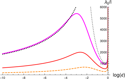
We calculate the scattering mean free path $\lambda_{\parallel}$ using Eqs. (14) and (16). We plot $\lambda_{\parallel}/l$ versus $\log(\varepsilon)$ in Fig. 10 for GS turbulence with $\mathcal{I}_{\rm A,S}=\mathcal{I}_{\rm A,S,1}$ and $R_{\rm n}=R_{\rm n,1}$. We use here the fitting formulae for $D_{\mu\mu}$ provided by Chandran (2000). The thick magenta solid line corresponds to $\delta=10^{-5}$, the red solid one to $\delta=3\times 10^{-5}$, and the orange dashed one to $\delta=10^{-4}$. $\lambda_{\parallel}/l$ grows with $\varepsilon$ at small $\varepsilon$. At such “small” values of $\delta$, $\lambda_{\parallel}/l$ reaches a peak and then decreases with $\varepsilon$. Chandran (2000) provided two formulae for the limiting behaviours of $\lambda_{\parallel}$ at small and large $\varepsilon$:

• For $\varepsilon^{3/2}\ll-\delta\ln\varepsilon$, i.e. at “small” $\varepsilon$ (black dotted line in Fig. 10),

  $$\frac{\lambda_{\parallel}}{l}\approx\frac{3\,(5/2-3\pi/4)}{-\delta\ln\varepsilon}\approx\frac{0.43}{-\delta\ln\varepsilon}\;.$$ (B1)

• For $\varepsilon^{3/2}\gg-\delta\ln\varepsilon$, i.e. at “large” $\varepsilon$ (grey dotted line in Fig. 10),

  $$\frac{\lambda_{\parallel}}{l}\approx 2.64\,(-\delta\ln\varepsilon)^{-5/11}\varepsilon^{-9/11}\;.$$ (B2)

Figure 10.— $\lambda_{\parallel}/l$ as a function of $\log(\varepsilon)$, for GS turbulence with $\mathcal{I}_{\rm A,S}=\mathcal{I}_{\rm A,S,1}$, $R_{\rm n}=R_{\rm n,1}$ (model A), and for 3 values of $\delta$: $\delta=10^{-5}$ (thick magenta solid line), $3\times 10^{-5}$ (red solid line), and $10^{-4}$ (orange dashed line). Dotted lines for the behaviours of $\lambda_{\parallel}/l$ at $\delta=10^{-5}$ in the limit of small or large $\varepsilon$, according to Chandran (2000): Eq. (B1) for $\varepsilon\ll-\delta\ln\varepsilon$ (black), and Eq. (B2) for $\varepsilon\gg-\delta\ln\varepsilon$ (grey).

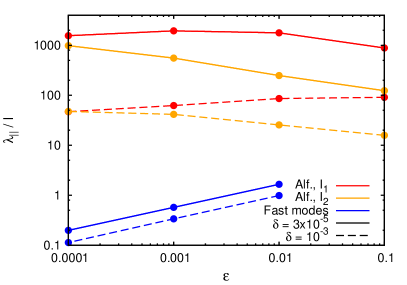
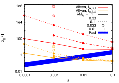
In Fig. 11, we plot $\lambda_{\parallel}/l$ versus $\varepsilon$, both for GS turbulence (red lines or symbols for $\mathcal{I}_{\rm A,S,1}$, orange for $\mathcal{I}_{\rm A,S,2}$) and for isotropic fast modes (blue lines or area). The left panel is for calculations made with the resonance function $R_{\rm n}=R_{\rm n,1}$, and the right panel is for $R_{\rm n}=R_{\rm n,2}$. Each line or symbol type corresponds to a different value of $\delta$ or $\delta\mathcal{M}_{\rm A}$, see keys.

Figure 11.— $\lambda_{\parallel}/l$ as a function of $\varepsilon$, for GS turbulence and for isotropic fast modes. Left panel: resonance function $R_{\rm n}=R_{\rm n,1}$ (models A, B & E). Right panel: $R_{\rm n}=R_{\rm n,2}$ (models C, D & F).

Appendix C Appendix C: Additional calculations of the scattering rate and anisotropy

We present in Fig. 12 calculations of $\nu=2D_{\mu\mu}/(1-\mu^{2})\times(l/v)$ (upper row) and $g(\mu)$ (lower row), for the cases whose parameters are within the shaded areas in Fig. 1 —except two points for GS turbulence with $\mathcal{I}_{\rm A,S}=\mathcal{I}_{\rm A,S,2}$ and $R_{\rm n}=R_{\rm n,2}$, which were studied in Sect. 3.1.4 ($\{\varepsilon,\delta\mathcal{M}_{\rm A}\}=\{10^{-3},0.33\}$ and $\{10^{-3},1\}$).

The left column in Fig. 12 is for GS turbulence with $\mathcal{I}_{\rm A,S}=\mathcal{I}_{\rm A,S,2}$ and $R_{\rm n}=R_{\rm n,1}$, the middle one for $\mathcal{I}_{\rm A,S,1}$ and $R_{\rm n,2}$, and the right one for $\mathcal{I}_{\rm A,S,2}$ and $R_{\rm n,2}$. Each column has its own set of line types and colors, sey keys for values of $\varepsilon$, $\delta$, or $\delta\mathcal{M}_{\rm A}$.

Figure 12.— $\nu$ (upper row) and $g$ (lower row) as functions of $\mu$, for the cases whose parameters are within the shaded areas in Fig. 1. GS turbulence with: $\mathcal{I}_{\rm A,S}=\mathcal{I}_{\rm A,S,2}$ and $R_{\rm n}=R_{\rm n,1}$ (left column), $\mathcal{I}_{\rm A,S,1}$ and $R_{\rm n,2}$ (middle column), and $\mathcal{I}_{\rm A,S,2}$ and $R_{\rm n,2}$ (right column). See keys for parameters: each column has its own set of line types and colors.

References

- Aartsen et al. (2013) Aartsen, M. G. et al. 2013, ApJ, 765, 55, arXiv:1210.5278
- Aartsen et al. (2016) ——. 2016, ApJ, 826, 220, arXiv:1603.01227
- Abbasi et al. (2012) Abbasi, R. et al. 2012, ApJ, 746, 33, arXiv:1109.1017
- Ahlers (2014) Ahlers, M. 2014, Physical Review Letters, 112, 021101, arXiv:1310.5712
- Ahlers (2016) ——. 2016, Physical Review Letters, 117, 151103, arXiv:1605.06446
- Ahlers et al. (2016) Ahlers, M., BenZvi, S. Y., Desiati, P., Díaz-Vélez, J. C., Fiorino, D. W., & Westerhoff, S. 2016, ApJ, 823, 10, arXiv:1601.07877
- Ahlers & Mertsch (2015) Ahlers, M., & Mertsch, P. 2015, ApJ, 815, L2, arXiv:1506.05488
- Battaner et al. (2015) Battaner, E., Castellano, J., & Masip, M. 2015, ApJ, 799, 157, arXiv:1407.0850
- Bethe et al. (1938) Bethe, H. A., Rose, M. E., & Smith, L. P. 1938, Proceedings of the American Philosophical Society, 78, 573
- Blasi & Amato (2012) Blasi, P., & Amato, E. 2012, JCAP, 1, 011, arXiv:1105.4529
- Burlaga & Ness (2016) Burlaga, L. F., & Ness, N. F. 2016, ApJ, 829, 134
- Chandran (2000) Chandran, B. D. G. 2000, Physical Review Letters, 85, 4656, arXiv:astro-ph/0008498
- Cho & Lazarian (2002) Cho, J., & Lazarian, A. 2002, Physical Review Letters, 88, 245001, arXiv:astro-ph/0205282
- Cho et al. (2002) Cho, J., Lazarian, A., & Vishniac, E. T. 2002, ApJ, 564, 291, arXiv:astro-ph/0105235
- Desiati & Lazarian (2013) Desiati, P., & Lazarian, A. 2013, ApJ, 762, 44, arXiv:1111.3075
- Di Sciascio & Iuppa (2014) Di Sciascio, G., & Iuppa, R. 2014, ArXiv e-prints, arXiv:1407.2144
- Díaz-Vélez et al. (2015) Díaz-Vélez, J. C., Fiorino, D., Desiati, P., Westerhoff, S., De la Fuente, E., The HAWC Collaboration, & The IceCube Collaboration. 2015, ArXiv e-prints, arXiv:1510.04134
- Drury (2013) Drury, L. 2013, ArXiv e-prints, arXiv:1305.6752
- Erlykin & Wolfendale (2006) Erlykin, A. D., & Wolfendale, A. W. 2006, Astroparticle Physics, 25, 183, arXiv:astro-ph/0601290
- Fisch & Kruskal (1980) Fisch, N. J., & Kruskal, M. D. 1980, J. Math. Phys., 21, 740
- Frisch et al. (2012) Frisch, P. C. et al. 2012, ApJ, 760, 106, arXiv:1206.1273
- Frisch et al. (2015) ——. 2015, ApJ, 814, 112, arXiv:1510.04679
- Funsten et al. (2009) Funsten, H. O. et al. 2009, Science, 326, 964
- Funsten et al. (2013) ——. 2013, ApJ, 776, 30
- Giacinti & Sigl (2012) Giacinti, G., & Sigl, G. 2012, Physical Review Letters, 109, 071101, arXiv:1111.2536
- Goldreich & Sridhar (1995) Goldreich, P., & Sridhar, S. 1995, ApJ, 438, 763
- Han et al. (2006) Han, J. L., Manchester, R. N., Lyne, A. G., Qiao, G. J., & van Straten, W. 2006, ApJ, 642, 868, arXiv:astro-ph/0601357
- Hasselmann & Wibberenz (1970) Hasselmann, K., & Wibberenz, G. 1970, ApJ, 162, 1049
- Haverkorn et al. (2008) Haverkorn, M., Brown, J. C., Gaensler, B. M., & McClure-Griffiths, N. M. 2008, ApJ, 680, 362, arXiv:0802.2740
- Heiles (1996) Heiles, C. 1996, ApJ, 462, 316
- Jokipii (1966) Jokipii, J. R. 1966, ApJ, 146, 480
- Jones et al. (1978) Jones, F. C., Birmingham, T. J., & Kaiser, T. B. 1978, Physics of Fluids, 21, 347
- Kirk et al. (2000) Kirk, J. G., Guthmann, A. W., Gallant, Y. A., & Achterberg, A. 2000, ApJ, 542, 235, arXiv:astro-ph/0005222
- Kulsrud & Pearce (1969) Kulsrud, R., & Pearce, W. P. 1969, ApJ, 156, 445
- Kumar & Eichler (2014) Kumar, R., & Eichler, D. 2014, ApJ, 785, 129
- López-Barquero et al. (2016) López-Barquero, V., Farber, R., Xu, S., Desiati, P., & Lazarian, A. 2016, ApJ, 830, 19, arXiv:1509.00892
- Malkov et al. (2010) Malkov, M. A., Diamond, P. H., O’C. Drury, L., & Sagdeev, R. Z. 2010, ApJ, 721, 750, arXiv:1005.1312
- Malkov & Sagdeev (2015) Malkov, M. A., & Sagdeev, R. Z. 2015, ApJ, 808, 157, arXiv:1502.01799
- Mertsch & Funk (2015) Mertsch, P., & Funk, S. 2015, Physical Review Letters, 114, 021101, arXiv:1408.3630
- Pohl & Eichler (2013) Pohl, M., & Eichler, D. 2013, ApJ, 766, 4, arXiv:1208.5338
- Schwadron et al. (2014) Schwadron, N. A. et al. 2014, Science, 343, 988
- Schwadron et al. (2009) ——. 2009, Science, 326, 966
- Sridhar & Goldreich (1994) Sridhar, S., & Goldreich, P. 1994, ApJ, 432, 612
- Vedenov et al. (1962) Vedenov, A. A., Velikhov, E. P., & Sagdeev, R. Z. 1962, Nuclear Fusion, 2, 465
- Völk (1973) Völk, H. J. 1973, Ap&SS, 25, 471
- Völk (1975) ——. 1975, Reviews of Geophysics and Space Physics, 13, 547
- Yan & Lazarian (2002) Yan, H., & Lazarian, A. 2002, Physical Review Letters, 89, 281102, arXiv:astro-ph/0205285
- Yan & Lazarian (2004) ——. 2004, ApJ, 614, 757, arXiv:astro-ph/0408172
- Yan & Lazarian (2008) ——. 2008, ApJ, 673, 942, arXiv:0710.2617
- Zhang et al. (2014) Zhang, M., Zuo, P., & Pogorelov, N. 2014, ApJ, 790, 5
- Zirnstein et al. (2016) Zirnstein, E. J., Heerikhuisen, J., Funsten, H. O., Livadiotis, G., McComas, D. J., & Pogorelov, N. V. 2016, ApJ, 818, L18