aainstitutetext: Department of Mathematics, Quaid-i-Azam University, Islamabad, Pakistanbbinstitutetext: Center for the Fundamental Laws of Nature, Harvard University, Cambridge, MA 02138, USA
institutetext: Electronic Address: jahmed@student.qau.edu.pk; ksaifullah@fas.harvard.edu

Greybody factor of scalar field from Reissner-Nordström-de Sitter black hole

Jamil Ahmed a,b    and K. Saifullah
Abstract

In this work we derive a general expression for the greybody factor of non-minimally coupled scalar fields in Reissner-Nordström-de Sitter spacetime in low frequency approximation. Greybody factor as a characteristic of effective potential barrier, will be presented. We discuss the role of cosmological constant both, in the absence as well as in the presence of non-minimal coupling. Considering non-minimal coupling as a mass term, its effect on the greybody factor will be discussed. We also elaborate the significance of the results by giving formulae of differential energy rate and general absorption cross section. The greybody factor gives insight into the spectrum of Hawking radiations.

1 Introduction

The study of asymptotically non-flat spacetime geometries received a lot of attention after it was discovered that our Universe has entered into a new phase of accelerated expansion S . Among these non-flat geometries de Sitter spacetime is of great interest due to its rich symmetries and also because it could incorporate the accelerated expansion of the Universe due to the presence of non-zero cosmological constant in the Einstein field equations. As predicted, the Universe is in continous expansion, so in far future it will pass through a de Sitter phase. Further, de Sitter geometry could also approximate the inflationary phase of our Universe A . The fact that all black hole spacetimes of Kerr-Newman family can be generalized to include a cosmological constant makes black hole de Sitter spacetimes an interesting field of investigation. De Sitter spacetime is the maximally symmetric Lorentzian space having positive curvature. In four dimensions the symmetry group is SO(1,4)𝑆𝑂14SO(1,4) and topology is R×S𝑅𝑆R\times S. Due to the structure of de Sitter spacetime inertial observers are surrounded by cosmological horizons, which are a characteristic of spacetimes having positive cosmological constant. Also dS/CFT correspondence enhances the interest in the study of de Sitter spacetimes as they provide connection with conformal field theories. The absorption and emission spectra of a Schwarzschild black hole was studied in Ref. NS . There has been a considerable interest in the study of greybody factor of scalar and fermionic radiations from asymptotically flat spacetimes and black strings C ; SD ; LSE ; YH ; SJ ; M ; JA ; SI ; IS ; MF ; WJ ; ahmed2017greybody .

Black hole emission and absorption phenomena is related to this important quantity known as greybody factor. It is this quantity that makes it different from emission and absorption of black body. The question is, how this quantity originated? It is generated by an effective potential barrier by black hole spacetimes. This potential quantum mechanically allows some of the radiation to transmit and remaining to reflect back. This leads to the frequency dependent greybody factor. Due to this factor black hole thermal radiation formula is different from the black body radiation formula. Greybody factor not only alters the thermal radiation formula but is also important to compute the partial absorption cross section of black holes B ; D ; W . In the literature there are investigations for greybody factor of scalar fields for Schwarzschild-de Sitter black hole. These include the cases of lowest partial modes in low energy regimes PJA ; TJR ; LAE ; PTN .

In this paper we use the simple matching technique to solve the radial equation resulting from the Klein Gordon equation in the background of the Riessner-Nordström-de Sitter black hole. In this method we divide the space into two regimes, namely near the black hole horizon and near the cosmological horizon and find solutions for radial equations in both the regimes separately. Then we stretch these solutions to an intermediate point rmsubscript𝑟𝑚r_{m}. The choice of rmsubscript𝑟𝑚r_{m} is such that

rh<rm, rc>rm and ωrm1,formulae-sequencesubscript𝑟subscript𝑟𝑚 subscript𝑟𝑐subscript𝑟𝑚 and 𝜔subscript𝑟𝑚much-less-than1r_{h}<r_{m},\text{ \ \ }r_{c}>r_{m}\text{ \ \ and }\omega r_{m}\ll 1, (1)

where rhsubscript𝑟r_{h} and rcsubscript𝑟𝑐r_{c} correspond to black hole and cosmological horizons respectively and ω𝜔\omega is the frequency.

The rest of the paper is organized as follows. In Section 2 we will discuss the Klein Gordon equation and the profile of effective potential in the background of Reissner-Nordström-de Sitter black hole. In Section 3 we compute the greybody factor, starting from near black hole horizon solution, near cosmological horizon solution, and then matching them at an intermediate point. This yields expressions for greybody factor and spectrum of Hawking radiations. At the end we make some concluding remarks.

2 Klein Gordon equation and profile of effective potential

The spacetime metric for Reissner-Nordström-de Sitter black hole is given by,

ds2=g(r)dt21g(r)dr2r2(dθ2+sin2θdφ2),𝑑superscript𝑠2𝑔𝑟𝑑superscript𝑡21𝑔𝑟𝑑superscript𝑟2superscript𝑟2𝑑superscript𝜃2superscript2𝜃𝑑superscript𝜑2ds^{2}=g(r)dt^{2}-\frac{1}{g(r)}dr^{2}-r^{2}\left(d\theta^{2}+\sin^{2}\theta d\varphi^{2}\right), (2)

where

g(r)=12Mr+Q2r2Λr23.𝑔𝑟12𝑀𝑟superscript𝑄2superscript𝑟2Λsuperscript𝑟23g(r)=1-\frac{2M}{r}+\frac{Q^{2}}{r^{2}}-\frac{\Lambda r^{2}}{3}. (3)

and related electromagnetic field is given by the four-potential

Aμ=Qrδμt.subscript𝐴𝜇𝑄𝑟superscriptsubscript𝛿𝜇𝑡A_{\mu}=\frac{Q}{r}\delta_{\mu}^{t}. (4)

Here M𝑀M is mass and Q𝑄Q is charge of the black hole. Introducing a dimensionless cosmological parameter λ=13ΛM2𝜆13Λsuperscript𝑀2\lambda=\frac{1}{3}\Lambda M^{2}, a dimensionless charge e=QM𝑒𝑄𝑀e=\frac{Q}{M} and dimensionless coordinates tt/M𝑡𝑡𝑀t\longrightarrow t/M, rr/M𝑟𝑟𝑀r\longrightarrow r/M. It is equivalent to putting M=1𝑀1M=1 ZS11 . The horizons are determined by the condition

12r+e2r2λr2=0.12𝑟superscript𝑒2superscript𝑟2𝜆superscript𝑟201-\frac{2}{r}+\frac{e^{2}}{r^{2}}-\lambda r^{2}=0. (5)

It is clear from above equation that in the special case of e=0𝑒0e=0, the black hole spacetimes exist for all λ0𝜆0\lambda\leqslant 0 and for 0<λ1270𝜆1270<\lambda\leqslant\frac{1}{27}.

Before going into detailed calculations of analytic result of greybody factor we comment about its validity. It is interesting to note that it is valid for arbitrary quantum number l𝑙l and coupling ξ𝜉\xi. On the other hand the accuracy of the result is guaranteed only if the two asymptotic regions overlap, which implies that it is only valid for small frequencies. Also the approximation which we have used is justified for “small” black holes (compared with characteristic dS scale) that is λ<<1much-less-than𝜆1\lambda<<1. Therefore the result of greybody factor is valid only in complementary regions of parameter space.

We consider a scalar field theory in which the field is either minimally or non-minimally coupled to gravity and described by the following action

𝒮=d4xg[RξRΦ2μΦμΦ].𝒮superscript𝑑4𝑥𝑔delimited-[]𝑅𝜉𝑅superscriptΦ2subscript𝜇Φsuperscript𝜇Φ\mathcal{S}=\int{d^{4}x\sqrt{-g}[R-\xi R\Phi^{2}-\partial_{\mu}\Phi\partial^{\mu}\Phi].} (6)

The equation of motion for the above theory can be written as

1gμ[ggμννΦ(t,r,θ,φ)]=4ξΛΦ.1𝑔subscript𝜇delimited-[]𝑔superscript𝑔𝜇𝜈subscript𝜈Φ𝑡𝑟𝜃𝜑4𝜉ΛΦ\frac{1}{\sqrt{-g}}\partial_{\mu}\left[\sqrt{-g}g^{\mu\nu}\partial_{\nu}\Phi(t,r,\theta,\varphi)\right]=-4\xi\Lambda\Phi. (7)

In above, we have used R=4Λ𝑅4ΛR=-4\Lambda and ξ𝜉\xi is a coupling constant determining the magnitude of coupling between the scalar and gravitational field, with ξ=0𝜉0\xi=0 corresponding to the minimal coupling. In matrix form the above line element can be written as

gμν=(g(r)00001g(r)0000r20000r2sin2θ).subscript𝑔𝜇𝜈𝑔𝑟00001𝑔𝑟0000superscript𝑟20000superscript𝑟2superscript2𝜃g_{\mu\nu}=\left(\begin{array}[]{cccc}g(r)&0&0&0\\ 0&-\frac{1}{g(r)}&0&0\\ 0&0&-r^{2}&0\\ 0&0&0&-r^{2}\sin^{2}\theta\end{array}\right). (8)

Also,

g=r2sinθ.𝑔superscript𝑟2𝜃\sqrt{-g}=r^{2}\sin\theta. (9)

Using these values in equation (7)7\left(\ref{3}\right), it takes the form

1r2sinθt(r2sinθg(r)tΦ)+1r2sinθr(r2sinθ(g(r))rΦ)+1r2sinθθ(sinθθΦ)1superscript𝑟2𝜃subscript𝑡superscript𝑟2𝜃𝑔𝑟subscript𝑡Φ1superscript𝑟2𝜃subscript𝑟superscript𝑟2𝜃𝑔𝑟subscript𝑟Φ1superscript𝑟2𝜃subscript𝜃𝜃subscript𝜃Φ\frac{1}{r^{2}\sin\theta}\partial_{t}\left(\frac{r^{2}\sin\theta}{g(r)}\partial_{t}\Phi\right)+\frac{1}{r^{2}\sin\theta}\partial_{r}\left(r^{2}\sin\theta\left(-g(r)\right)\partial_{r}\Phi\right)+\frac{1}{r^{2}\sin\theta}\partial_{\theta}\left(-\sin\theta\partial_{\theta}\Phi\right)
+1r2sinθφ(φΦ)=4ξΛΦ.1superscript𝑟2𝜃subscript𝜑subscript𝜑Φ4𝜉ΛΦ+\frac{1}{r^{2}\sin\theta}\partial_{\varphi}\left(\partial_{\varphi}\Phi\right)=-4\xi\Lambda\Phi. (10)

Let

Φ(t,r,θ,φ)=eιωtR(r)Y(θ,φ),Φ𝑡𝑟𝜃𝜑superscript𝑒𝜄𝜔𝑡𝑅𝑟𝑌𝜃𝜑\Phi(t,r,\theta,\varphi)=e^{-\iota\omega t}R(r)Y(\theta,\varphi), (11)

therefore, the radial part of equation (10)10\left(\ref{7}\right) is

1r2ddr(r2g(r))dR(r)dr+[ω2g(r)l(l+1)r2+4ξΛ]R(r)=0,1superscript𝑟2𝑑𝑑𝑟superscript𝑟2𝑔𝑟𝑑𝑅𝑟𝑑𝑟delimited-[]superscript𝜔2𝑔𝑟𝑙𝑙1superscript𝑟24𝜉Λ𝑅𝑟0\frac{1}{r^{2}}\frac{d}{dr}\left(r^{2}g(r)\right)\frac{dR(r)}{dr}+\left[\frac{\omega^{2}}{g(r)}-\frac{l(l+1)}{r^{2}}+4\xi\Lambda\right]R(r)=0, (12)

where l(l+1)𝑙𝑙1l(l+1) are the eigenvalues coming from the (θ,φ)𝜃𝜑(\theta,\varphi) part.

Before solving equation (12)12\left(\ref{9}\right) we will discuss the profile of effective potential due to which greybody factor originates. We employ the following transformation on equation (12)12\left(\ref{9}\right)

R(r)=U(r)r𝑅𝑟𝑈𝑟𝑟R\left(r\right)=\frac{U\left(r\right)}{r} (13)

and the tortoise coordinate

xdrg,𝑥𝑑𝑟𝑔x\equiv\int\frac{dr}{g}, (14)

such that

ddx=gddr,d2dx2=g2d2dr2+ggddr.formulae-sequence𝑑𝑑𝑥𝑔𝑑𝑑𝑟superscript𝑑2𝑑superscript𝑥2superscript𝑔2superscript𝑑2𝑑superscript𝑟2𝑔superscript𝑔𝑑𝑑𝑟\frac{d}{dx}=g\frac{d}{dr},\frac{d^{2}}{dx^{2}}=g^{2}\frac{d^{2}}{dr^{2}}+gg^{\prime}\frac{d}{dr}.

Thus equation (12)12\left(\ref{9}\right) takes the form

(d2dx2+ω2Veff(r))U(r)=0,superscript𝑑2𝑑superscript𝑥2superscript𝜔2subscript𝑉𝑒𝑓𝑓𝑟𝑈𝑟0\left(\frac{d^{2}}{dx^{2}}+\omega^{2}-V_{eff}\left(r\right)\right)U\left(r\right)=0, (15)

with

Veff(r)=g(r)(l(l+1)r24ξΛ+gr).subscript𝑉𝑒𝑓𝑓𝑟𝑔𝑟𝑙𝑙1superscript𝑟24𝜉Λsuperscript𝑔𝑟V_{eff}\left(r\right)=g\left(r\right)\left(\frac{l\left(l+1\right)}{r^{2}}-4\xi\Lambda+\frac{g^{\prime}}{r}\right). (16)
Refer to caption
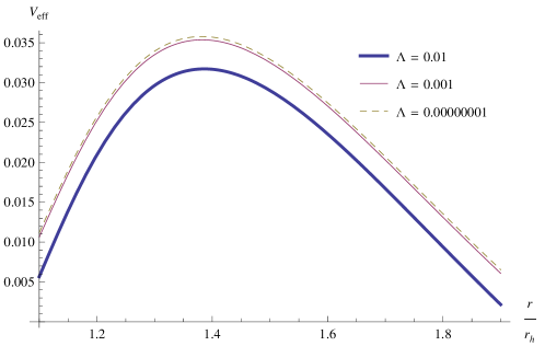
Figure 1: Profile of effective potential for different values of the cosmological constant for ξ=0.01𝜉0.01\xi=0.01, q=1𝑞1q=1 and l=0𝑙0l=0
Refer to caption
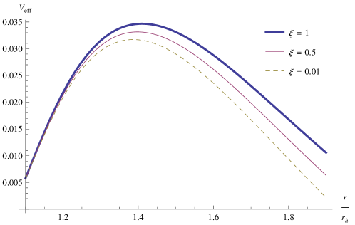
Figure 2: Profile of effective potential for different values of the coupling constant for Λ=0.01Λ0.01\Lambda=0.01, q=1𝑞1q=1 and l=0𝑙0l=0

In Fig. 1, we draw the profile of effective potential for different values of the cosmological constant for ξ=0.01𝜉0.01\xi=0.01, q=1𝑞1q=1 and l=0𝑙0l=0. It is observed that an increase in the value of cosmological constant, decreases the height of gravitational barrier and thus enhances the greybody factor. In Fig. 2, the effective potential is depicted for different values of the coupling constant and Λ=0.01Λ0.01\Lambda=0.01, q=1𝑞1q=1 and l=0𝑙0l=0. It is observed that increase in the value of the coupling constant leads to the increase in gravitational barrier, which subsequently suppresses the emission of scalar fields.

3 Greybody factor computation

3.1 Near black hole horizon solution

Equation (12)12\left(\ref{9}\right) is the master equation of our interest. We will solve this equation in two regions separately, namely, near the black hole horizon and the cosmological horizon by using a semi-classical approach known as simple matching technique. Then we will match both the solutions to an intermediate region to get the analytical expression for the greybody factor.

For the near horizon region rrhsimilar-to𝑟subscript𝑟r\sim r_{h}, we will perform the following transformation to simplify the radial equation PTN

rf=g(r)1Ξr2,𝑟𝑓𝑔𝑟1Ξsuperscript𝑟2r\rightarrow f=\frac{g\left(r\right)}{1-\Xi r^{2}}, (17)

where

Ξ=Λ3.ΞΛ3\Xi=\frac{\Lambda}{3}.

Thus we get

dfdr=(1f)B(rh)rh(1Ξrh2),\frac{df}{dr}=\left(1-f\right)\frac{B(r_{h)}}{r_{h}\left(1-\Xi r_{h}^{2}\right)}, (18)

where, in the above

B(rh)=(6ΛMrh3+4ΛQ2rh2+6Mrh6Q26Mrh3Q2).B(r_{h)}=\left(\frac{-6\Lambda Mr_{h}^{3}+4\Lambda Q^{2}r_{h}^{2}+6Mr_{h}-6Q^{2}}{6Mr_{h}-3Q^{2}}\right). (19)

Using equations (17)17\left(\ref{14}\right) and (18)18\left(\ref{15}\right) in (12)12\left(\ref{9}\right), we obtain

f(1f)d2R(f)df2+(1Cf)dR(f)df+[F2B2(rh)(1f)fλh(1Ξrh2)B2(rh)(1f)]R(f)=0.f(1-f)\frac{d^{2}R(f)}{df^{2}}+\left(1-C_{\ast}f\right)\frac{dR(f)}{df}+\left[\frac{F_{\ast}^{2}}{B^{2}(r_{h)}\left(1-f\right)f}-\frac{\lambda_{h}\left(1-\Xi r^{2}_{h}\right)}{B^{2}(r_{h)}\left(1-f\right)}\right]R(f)=0. (20)

Here

F=ωrh,subscript𝐹𝜔subscript𝑟F_{\ast}=\omega r_{h}, (21)
C=rh(1Ξrh2)(1f)2B(rh)2rh2Ξ(1Ξrh2)(1f)B(rh),subscript𝐶subscript𝑟1Ξsubscriptsuperscript𝑟2superscript1𝑓2𝐵subscript𝑟2superscriptsubscript𝑟2Ξ1Ξsubscriptsuperscript𝑟21𝑓𝐵subscript𝑟C_{\ast}=\frac{r_{h}\left(1-\Xi r^{2}_{h}\right)}{\left(1-f\right)^{2}B\left(r_{h}\right)}-\frac{2r_{h}^{2}\Xi\left(1-\Xi r^{2}_{h}\right)}{\left(1-f\right)B\left(r_{h}\right)}, (22)

and

λh=[l(l+1)4ξΛ]rh2.subscript𝜆delimited-[]𝑙𝑙14𝜉Λsuperscriptsubscript𝑟2\lambda_{h}=\left[l\left(l+1\right)-4\xi\Lambda\right]r_{h}^{2}. (23)

In order to further simplify the above equation we use field redefinition

R(f)=fμ1(1f)ν1F(f).𝑅𝑓superscript𝑓subscript𝜇1superscript1𝑓subscript𝜈1𝐹𝑓R(f)=f^{\mu_{1}}\left(1-f\right)^{\nu_{1}}F(f). (24)

In equation (20)20\left(\ref{17}\right) we use this definition of R(f)𝑅𝑓R(f) to get

f(1f)d2F(f)df2+[1+2μ1(2μ1+2ν1+C)f]dFdf+(μ12fμ12+μ12μ1ν1+ν121fν122ν11ff\left(1-f\right)\frac{d^{2}F(f)}{df^{2}}+\left[1+2\mu_{1}-\left(2\mu_{1}+2\nu_{1}+C_{\ast}\right)f\right]\frac{dF}{df}+(\frac{\mu_{1}^{2}}{f}-\mu_{1}^{2}+\mu_{1}-2\mu_{1}\nu_{1}+\frac{\nu_{1}^{2}}{1-f}-\nu_{1}^{2}-\frac{2\nu_{1}}{1-f}
+ν1μ1C+ν1C1fν1C+F2B2(rh)f+F2B2(rh)(1f)λh(1Ξrh2)B2(rh)(1f))F(f)=0+\nu_{1}-\mu_{1}C_{\ast}+\frac{\nu_{1}C_{\ast}}{1-f}-\nu_{1}C_{\ast}+\frac{F_{\ast}^{2}}{B^{2}(r_{h})f}+\frac{F_{\ast}^{2}}{B^{2}(r_{h})\left(1-f\right)}-\frac{\lambda_{h}\left(1-\Xi r^{2}_{h}\right)}{B^{2}(r_{h)}\left(1-f\right)})F(f)=0 (25)

Now, define

a1=μ1+ν1+C1,subscript𝑎1subscript𝜇1subscript𝜈1subscript𝐶1a_{1}=\mu_{1}+\nu_{1}+C_{\ast}-1, (26)
b1=μ1+ν1,subscript𝑏1subscript𝜇1subscript𝜈1b_{1}=\mu_{1}+\nu_{1}, (27)
c1=1+2μ1.subscript𝑐112subscript𝜇1c_{1}=1+2\mu_{1}. (28)

Also constraints coming from the coefficients of F(f)𝐹𝑓F(f) give

μ12+F2B2(rh)=0,superscriptsubscript𝜇12superscriptsubscript𝐹2superscript𝐵2subscript𝑟0\mu_{1}^{2}+\frac{F_{\ast}^{2}}{B^{2}(r_{h})}=0, (29)

and

ν12+ν1(C2)+F2B2(rh)λh(1Ξrh2)B2(rh)=0.\nu_{1}^{2}+\nu_{1}(C_{\ast}-2)+\frac{F_{\ast}^{2}}{B^{2}(r_{h})}-\frac{\lambda_{h}\left(1-\Xi r^{2}_{h}\right)}{B^{2}(r_{h)}}=0. (30)

From here we find the values of μ1subscript𝜇1\mu_{1} and ν1subscript𝜈1\nu_{1} as

μ1=±ιFB(rh),subscript𝜇1plus-or-minus𝜄subscript𝐹𝐵subscript𝑟\mu_{1}=\pm\iota\frac{F_{\ast}}{B(r_{h})}, (31)

and

ν1=12[(2C)±(2C)24(F2B2(rh)4λh(1Ξrh2)λhB2(rh))].\nu_{1}=\frac{1}{2}\left[\left(2-C_{\ast}\right)\pm\sqrt{\left(2-C_{\ast}\right)^{2}-4\left(\frac{F_{\ast}^{2}}{B^{2}(r_{h})}-\frac{4\lambda_{h}\left(1-\Xi r^{2}_{h}\right)\lambda_{h}}{B^{2}(r_{h)}}\right)}\right]. (32)

Thus equation (25)25\left(\ref{22}\right) by virtue of equations (26,27,28)262728\left(\ref{23},\ref{23a},\ref{23b}\right) and constraints (29,30)2930\left(\ref{24},\ref{25}\right) becomes

f(1f)d2F(f)df2+[c1(1+a1+b1)f]dF(f)dfa1b1F(f)=0.𝑓1𝑓superscript𝑑2𝐹𝑓𝑑superscript𝑓2delimited-[]subscript𝑐11subscript𝑎1subscript𝑏1𝑓𝑑𝐹𝑓𝑑𝑓subscript𝑎1subscript𝑏1𝐹𝑓0f\left(1-f\right)\frac{d^{2}F(f)}{df^{2}}+\left[c_{1}-\left(1+a_{1}+b_{1}\right)f\right]\frac{dF(f)}{df}-a_{1}b_{1}F(f)=0. (33)

In the near horizon region the solution can be written in the form of general hypergeometric function, which has the form

R(f)NH=A1fμ1(1f)ν1F(a,b,c;f)+A2fμ1(1f)ν1F(ac+1,bc+1,2c;f)𝑅subscript𝑓𝑁𝐻subscript𝐴1superscript𝑓subscript𝜇1superscript1𝑓subscript𝜈1𝐹𝑎𝑏𝑐𝑓subscript𝐴2superscript𝑓subscript𝜇1superscript1𝑓subscript𝜈1𝐹𝑎𝑐1𝑏𝑐12𝑐𝑓R(f)_{NH}=A_{1}f^{\mu_{1}}(1-f)^{\nu_{1}}F\left(a,b,c;f\right)+A_{2}f^{-\mu_{1}}(1-f)^{\nu_{1}}F\left(a-c+1,b-c+1,2-c;f\right) (34)

where A1 subscript𝐴1 A_{1\text{ }}and A2subscript𝐴2A_{2} are arbitrary constants. For the near horizon case there exists no outgoing mode, we choose A2=0subscript𝐴20A_{2}=0, thus we get

R(f)NH=A1fμ1(1f)ν1F(a,b,c;f).𝑅subscript𝑓𝑁𝐻subscript𝐴1superscript𝑓subscript𝜇1superscript1𝑓subscript𝜈1𝐹𝑎𝑏𝑐𝑓R(f)_{NH}=A_{1}f^{\mu_{1}}(1-f)^{\nu_{1}}F\left(a,b,c;f\right). (35)

3.2 Near cosmological horizon solution

We now solve the radial equation (12)12\left(\ref{9}\right) close to the cosmological horizon rcsubscript𝑟𝑐r_{c}. In this case we choose the radial function h(r)𝑟h\left(r\right), in place of g(r)𝑔𝑟g\left(r\right), which is defined as

h(r)=1Ξr2.𝑟1Ξsuperscript𝑟2h\left(r\right)=1-\Xi r^{2}. (36)

We employ the following transformation on equation (12)12\left(\ref{9}\right)

rh(r),𝑟𝑟r\rightarrow h\left(r\right), (37)

so that


dhdr=(1h)r(2).𝑑𝑑𝑟1𝑟2\frac{dh}{dr}=\frac{\left(1-h\right)}{r}\left(-2\right). (38)

Using this, equation (12)12\left(\ref{9}\right) becomes

h(1h)d2R(h)dh2+(12h)dR(h)dh+[Fc2Bc2(1h)hλc(1h)Bc2]R(h)=0,1superscript𝑑2𝑅𝑑superscript212𝑑𝑅𝑑delimited-[]superscriptsubscript𝐹𝑐2superscriptsubscript𝐵𝑐21subscript𝜆𝑐1superscriptsubscript𝐵𝑐2𝑅0h(1-h)\frac{d^{2}R(h)}{dh^{2}}+\left(1-2h\right)\frac{dR(h)}{dh}+\left[\frac{F_{c}^{2}}{B_{c}^{2}\left(1-h\right)h}-\frac{\lambda_{c}}{\left(1-h\right)B_{c}^{2}}\right]R(h)=0, (39)

where, Fc=ωrc2subscript𝐹𝑐𝜔superscriptsubscript𝑟𝑐2F_{c}=\omega r_{c}^{2}, Bc=2subscript𝐵𝑐2B_{c}=-2 and λc=[l(l+1)4ξΛ]rc2subscript𝜆𝑐delimited-[]𝑙𝑙14𝜉Λsuperscriptsubscript𝑟𝑐2\lambda_{c}=\left[l\left(l+1\right)-4\xi\Lambda\right]r_{c}^{2}. We redefine the radial function as

R(h)=hμ2(1h)ν2X(h).𝑅superscriptsubscript𝜇2superscript1subscript𝜈2𝑋R(h)=h^{\mu_{2}}\left(1-h\right)^{\nu_{2}}X\left(h\right). (40)

Using equation (40)40\left(\ref{34a}\right) in (39)39\left(\ref{33a}\right) it takes the form

h(1h)d2X(h)dh2+[c2(1+a2+b2)f]dX(h)dha2b2X(h)=0.1superscript𝑑2𝑋𝑑superscript2delimited-[]subscript𝑐21subscript𝑎2subscript𝑏2𝑓𝑑𝑋𝑑subscript𝑎2subscript𝑏2𝑋0h\left(1-h\right)\frac{d^{2}X(h)}{dh^{2}}+\left[c_{2}-\left(1+a_{2}+b_{2}\right)f\right]\frac{dX(h)}{dh}-a_{2}b_{2}X(h)=0. (41)

In the above we defined

a2=μ2+ν2+1,subscript𝑎2subscript𝜇2subscript𝜈21a_{2}=\mu_{2}+\nu_{2}+1, (42)
b2=μ2+ν2,subscript𝑏2subscript𝜇2subscript𝜈2b_{2}=\mu_{2}+\nu_{2}, (43)
c2=1+2μ2.subscript𝑐212subscript𝜇2c_{2}=1+2\mu_{2}. (44)

Also the constraints coming from the coefficients of X(h)𝑋X\left(h\right) are

μ22+Fc2Bc2=0superscriptsubscript𝜇22superscriptsubscript𝐹𝑐2superscriptsubscript𝐵𝑐20\mu_{2}^{2}+\frac{F_{c}^{2}}{B_{c}^{2}}=0 (45)

and

ν22+Fc2Bc2λcBc2=0.superscriptsubscript𝜈22superscriptsubscript𝐹𝑐2superscriptsubscript𝐵𝑐2subscript𝜆𝑐superscriptsubscript𝐵𝑐20\nu_{2}^{2}+\frac{F_{c}^{2}}{B_{c}^{2}}-\frac{\lambda_{c}}{B_{c}^{2}}=0. (46)

From the above two equations we obtain the values of power coefficients as

μ2±=±ιFcBc,ν2±=±Fc2Bc2λcBc2.formulae-sequencesubscript𝜇limit-from2plus-or-minusplus-or-minus𝜄subscript𝐹𝑐subscript𝐵𝑐subscript𝜈limit-from2plus-or-minusplus-or-minussuperscriptsubscript𝐹𝑐2superscriptsubscript𝐵𝑐2subscript𝜆𝑐superscriptsubscript𝐵𝑐2\mu_{2\pm}=\pm\iota\frac{F_{c}}{B_{c}},\nu_{2\pm}=\pm\sqrt{\frac{F_{c}^{2}}{B_{c}^{2}}-\frac{\lambda_{c}}{B_{c}^{2}}}. (47)

Equation (41)41\left(\ref{35a}\right) is again a hypergeometric equation and in order to ensure the convergence of the hypergeometric function, we choose negative sign of ν2subscript𝜈2\nu_{2}. Near the cosmological constant both the modes, incoming and outgoing exist, so the general solution can be written as

R(h)CH=B1hμ2(1h)ν2F(a2,b2,c2;h)+B2hμ2(1h)ν2F(a2c2+1,b2c2+1,2c2;h).𝑅subscript𝐶𝐻subscript𝐵1superscriptsubscript𝜇2superscript1subscript𝜈2𝐹subscript𝑎2subscript𝑏2subscript𝑐2subscript𝐵2superscriptsubscript𝜇2superscript1subscript𝜈2𝐹subscript𝑎2subscript𝑐21subscript𝑏2subscript𝑐212subscript𝑐2R(h)_{CH}=B_{1}h^{\mu_{2}}(1-h)^{\nu_{2}}F\left(a_{2},b_{2},c_{2};h\right)+B_{2}h^{-\mu_{2}}(1-h)^{\nu_{2}}F\left(a_{2}-c_{2}+1,b_{2}-c_{2}+1,2-c_{2};h\right). (48)

3.3 Matching to an intermediate region

In order to match the above two solutions of the radial equation i.e., near horizon and near cosmological horizon solutions, to an intermediate region we use matching technique. We first shift the near horizon solution given in equation (35)35\left(\ref{30}\right) to an intermediate region, for which we change the argument of the hypergeometric function from f𝑓f to 1f1𝑓1-f . This gives the following SJ ; MI .

R(f)NH=A1fμ1(1f)ν1{Γ(c1)Γ(c1a1b1)Γ(ca)Γ(cb)F(a1,b1,a1+b1c1+1;1f)R(f)_{NH}=A_{1}f^{\mu_{1}}\left(1-f\right)^{\nu_{1}}{\Huge\{}\frac{\Gamma(c_{1})\Gamma(c_{1}-a_{1}-b_{1})}{\Gamma(c-a)\Gamma(c-b)}F\left(a_{1},b_{1},a_{1}+b_{1}-c_{1}+1;1-f\right)
+(1f)c1a1b1Γ(c1)Γ(a1+b1c1)Γ(a1)Γ(b1)F(c1a1,c1b1,c1a1b1+1;1f)}.+\left(1-f\right)^{c_{1}-a_{1}-b_{1}}\frac{\Gamma(c_{1})\Gamma(a_{1}+b_{1}-c_{1})}{\Gamma(a_{1})\Gamma(b_{1})}F\left(c_{1}-a_{1},c_{1}-b_{1},c_{1}-a_{1}-b_{1}+1;1-f\right){\Huge\}}. (49)

In the limit rrhmuch-greater-than𝑟subscript𝑟r\gg r_{h}, f1𝑓1f\rightarrow 1 and we can use

(1f)ν1(rhr)ν1(rrh)l,similar-to-or-equalssuperscript1𝑓subscript𝜈1superscriptsubscript𝑟𝑟subscript𝜈1similar-to-or-equalssuperscript𝑟subscript𝑟𝑙\left(1-f\right)^{\nu_{1}}\simeq\left(\frac{r_{h}}{r}\right)^{\nu_{1}}\simeq\left(\frac{r}{r_{h}}\right)^{l}, (50)

and

(1f)ν1+c1a1b1(rhr)2Bhν1(rrh)(l+1).similar-to-or-equalssuperscript1𝑓subscript𝜈1subscript𝑐1subscript𝑎1subscript𝑏1superscriptsubscript𝑟𝑟2subscript𝐵subscript𝜈1similar-to-or-equalssuperscript𝑟subscript𝑟𝑙1\left(1-f\right)^{\nu_{1}+c_{1}-a_{1}-b_{1}}\simeq\left(\frac{r_{h}}{r}\right)^{2-B_{h}-\nu_{1}}\simeq\left(\frac{r}{r_{h}}\right)^{-\left(l+1\right)}. (51)

So, in an intermediate region the solution will take the following form

R(r)BH=A1Γ(c1)Γ(c1a1b1)Γ(c1a1)Γ(c1b1)(rrh)l+A1Γ(c1)Γ(a1+b1c1)Γ(a1)Γ(b1)(rrh)(l+1),𝑅subscript𝑟𝐵𝐻subscript𝐴1Γsubscript𝑐1Γsubscript𝑐1subscript𝑎1subscript𝑏1Γsubscript𝑐1subscript𝑎1Γsubscript𝑐1subscript𝑏1superscript𝑟subscript𝑟𝑙subscript𝐴1Γsubscript𝑐1Γsubscript𝑎1subscript𝑏1subscript𝑐1Γsubscript𝑎1Γsubscript𝑏1superscript𝑟subscript𝑟𝑙1R(r)_{BH}=A_{1}\frac{\Gamma(c_{1})\Gamma(c_{1}-a_{1}-b_{1})}{\Gamma(c_{1}-a_{1})\Gamma(c_{1}-b_{1})}\left(\frac{r}{r_{h}}\right)^{l}+A_{1}\frac{\Gamma(c_{1})\Gamma(a_{1}+b_{1}-c_{1})}{\Gamma(a_{1})\Gamma(b_{1})}\left(\frac{r}{r_{h}}\right)^{-\left(l+1\right)}, (52)

or

R(r)BH=ϝ1r(l+1)+ϝ2rl.𝑅subscript𝑟𝐵𝐻subscriptitalic-ϝ1superscript𝑟𝑙1subscriptitalic-ϝ2superscript𝑟𝑙R(r)_{BH}=\digamma_{1}r^{-\left(l+1\right)}+\digamma_{2}r^{l}. (53)

In the above we have used

ϝ1=A1Γ(c1)Γ(a1+b1c1)Γ(a1)Γ(b1),subscriptitalic-ϝ1subscript𝐴1Γsubscript𝑐1Γsubscript𝑎1subscript𝑏1subscript𝑐1Γsubscript𝑎1Γsubscript𝑏1\digamma_{1}=A_{1}\frac{\Gamma(c_{1})\Gamma(a_{1}+b_{1}-c_{1})}{\Gamma(a_{1})\Gamma(b_{1})}, (54)
ϝ2=A1Γ(c1)Γ(c1a1b1)Γ(c1a1)Γ(c1b1).subscriptitalic-ϝ2subscript𝐴1Γsubscript𝑐1Γsubscript𝑐1subscript𝑎1subscript𝑏1Γsubscript𝑐1subscript𝑎1Γsubscript𝑐1subscript𝑏1\digamma_{2}=A_{1}\frac{\Gamma(c_{1})\Gamma(c_{1}-a_{1}-b_{1})}{\Gamma(c_{1}-a_{1})\Gamma(c_{1}-b_{1})}. (55)

Now we turn to equation (48)48\left(\ref{40a}\right) and shift its argument of hypergeometric function from hh to 1h.11-h. Thus near cosmological horizon, we have h(rc)0subscript𝑟𝑐0h(r_{c})\rightarrow 0, therefore

(1h)ν2(rrc)ν2(rrc)(l+1),similar-to-or-equalssuperscript1subscript𝜈2superscript𝑟subscript𝑟𝑐subscript𝜈2similar-to-or-equalssuperscript𝑟subscript𝑟𝑐𝑙1\left(1-h\right)^{\nu_{2}}\simeq\left(\frac{r}{r_{c}}\right)^{\nu_{2}}\simeq\left(\frac{r}{r_{c}}\right)^{-\left(l+1\right)}, (56)

and

(1h)ν2+c2a2b2(rrc)(1+2ν2)(rrc)l.similar-to-or-equalssuperscript1subscript𝜈2subscript𝑐2subscript𝑎2subscript𝑏2superscript𝑟subscript𝑟𝑐12subscript𝜈2similar-to-or-equalssuperscript𝑟subscript𝑟𝑐𝑙\left(1-h\right)^{\nu_{2}+c_{2}-a_{2}-b_{2}}\simeq\left(\frac{r}{r_{c}}\right)^{-\left(1+2\nu_{2}\right)}\simeq\left(\frac{r}{r_{c}}\right)^{l}. (57)

By using the above approximations and properties of hypergeometric functions MI we can write equation (53)53(\ref{45a}) as

R(r)C=[B1Γ(c2)Γ(c2a2b2)Γ(c2a2)Γ(c2b2)+B2Γ(2c2)Γ(c2a2b2)Γ(1a2)Γ(1b2)](rrc)(l+1)𝑅subscript𝑟𝐶delimited-[]subscript𝐵1Γsubscript𝑐2Γsubscript𝑐2subscript𝑎2subscript𝑏2Γsubscript𝑐2subscript𝑎2Γsubscript𝑐2subscript𝑏2subscript𝐵2Γ2subscript𝑐2Γsubscript𝑐2subscript𝑎2subscript𝑏2Γ1subscript𝑎2Γ1subscript𝑏2superscript𝑟subscript𝑟𝑐𝑙1R(r)_{C}=\left[B_{1}\frac{\Gamma(c_{2})\Gamma(c_{2}-a_{2}-b_{2})}{\Gamma(c_{2}-a_{2})\Gamma(c_{2}-b_{2})}+B_{2}\frac{\Gamma(2-c_{2})\Gamma(c_{2}-a_{2}-b_{2})}{\Gamma(1-a_{2})\Gamma(1-b_{2})}\right]\left(\frac{r}{r_{c}}\right)^{-\left(l+1\right)}
[B1Γ(c2)Γ(a2+b2c2)Γ(a2)Γ(b2)+B2Γ(2c2)Γ(a2b2c2)Γ(a2+1c2)Γ(b2+1c2)](rrc)l,delimited-[]subscript𝐵1Γsubscript𝑐2Γsubscript𝑎2subscript𝑏2subscript𝑐2Γsubscript𝑎2Γsubscript𝑏2subscript𝐵2Γ2subscript𝑐2Γsubscript𝑎2subscript𝑏2subscript𝑐2Γsubscript𝑎21subscript𝑐2Γsubscript𝑏21subscript𝑐2superscript𝑟subscript𝑟𝑐𝑙\left[B_{1}\frac{\Gamma(c_{2})\Gamma(a_{2}+b_{2}-c_{2})}{\Gamma(a_{2})\Gamma(b_{2})}+B_{2}\frac{\Gamma(2-c_{2})\Gamma(a_{2}-b_{2}-c_{2})}{\Gamma(a_{2}+1-c_{2})\Gamma(b_{2}+1-c_{2})}\right]\left(\frac{r}{r_{c}}\right)^{l}, (58)

or

R(r)C=(ϝ3B1+ϝ4B2)(rrc)(l+1)+(ϝ5B1+ϝ6B2)(rrc)l.𝑅subscript𝑟𝐶subscriptitalic-ϝ3subscript𝐵1subscriptitalic-ϝ4subscript𝐵2superscript𝑟subscript𝑟𝑐𝑙1subscriptitalic-ϝ5subscript𝐵1subscriptitalic-ϝ6subscript𝐵2superscript𝑟subscript𝑟𝑐𝑙R(r)_{C}=\left(\digamma_{3}B_{1}+\digamma_{4}B_{2}\right)\left(\frac{r}{r_{c}}\right)^{-\left(l+1\right)}+\left(\digamma_{5}B_{1}+\digamma_{6}B_{2}\right)\left(\frac{r}{r_{c}}\right)^{l}. (59)

Here we have used

ϝ3=Γ(c2)Γ(c2a2b2)Γ(c2a2)Γ(c2b2),ϝ4=Γ(2c2)Γ(c2a2b2)Γ(1a2)Γ(1b2),formulae-sequencesubscriptitalic-ϝ3Γsubscript𝑐2Γsubscript𝑐2subscript𝑎2subscript𝑏2Γsubscript𝑐2subscript𝑎2Γsubscript𝑐2subscript𝑏2subscriptitalic-ϝ4Γ2subscript𝑐2Γsubscript𝑐2subscript𝑎2subscript𝑏2Γ1subscript𝑎2Γ1subscript𝑏2\digamma_{3}=\frac{\Gamma(c_{2})\Gamma(c_{2}-a_{2}-b_{2})}{\Gamma(c_{2}-a_{2})\Gamma(c_{2}-b_{2})},\digamma_{4}=\frac{\Gamma(2-c_{2})\Gamma(c_{2}-a_{2}-b_{2})}{\Gamma(1-a_{2})\Gamma(1-b_{2})}, (60)
ϝ5=Γ(c2)Γ(a2+b2c2)Γ(a2)Γ(b2),ϝ6=Γ(2c2)Γ(a2b2c2)Γ(a2+1c2)Γ(b2+1c2).formulae-sequencesubscriptitalic-ϝ5Γsubscript𝑐2Γsubscript𝑎2subscript𝑏2subscript𝑐2Γsubscript𝑎2Γsubscript𝑏2subscriptitalic-ϝ6Γ2subscript𝑐2Γsubscript𝑎2subscript𝑏2subscript𝑐2Γsubscript𝑎21subscript𝑐2Γsubscript𝑏21subscript𝑐2\digamma_{5}=\frac{\Gamma(c_{2})\Gamma(a_{2}+b_{2}-c_{2})}{\Gamma(a_{2})\Gamma(b_{2})},\digamma_{6}=\frac{\Gamma(2-c_{2})\Gamma(a_{2}-b_{2}-c_{2})}{\Gamma(a_{2}+1-c_{2})\Gamma(b_{2}+1-c_{2})}. (61)

3.4 Greybody factor

Greybody factor for the emission of scalar fields can be defined by the amplitudes of the waves at the stretched cosmological horizon solution PTN that is

|Al|2=1|B2B1|2.superscriptsubscript𝐴𝑙21superscriptsubscript𝐵2subscript𝐵12\left|A_{l}\right|^{2}=1-\left|\frac{B_{2}}{B_{1}}\right|^{2}. (62)

As the power law in (53)53\left(\ref{45a}\right) and (59)59\left(\ref{51a}\right) is same, we match these two solutions to get the values of B1subscript𝐵1B_{1} and B2subscript𝐵2B_{2} as

B1=ϝ1ϝ6ϝ2ϝ4ϝ3ϝ6ϝ4ϝ5,subscript𝐵1subscriptitalic-ϝ1subscriptitalic-ϝ6subscriptitalic-ϝ2subscriptitalic-ϝ4subscriptitalic-ϝ3subscriptitalic-ϝ6subscriptitalic-ϝ4subscriptitalic-ϝ5B_{1}=\frac{\digamma_{1}\digamma_{6}-\digamma_{2}\digamma_{4}}{\digamma_{3}\digamma_{6}-\digamma_{4}\digamma_{5}}, (63)
B2=ϝ2ϝ3ϝ1ϝ5ϝ3ϝ6ϝ4ϝ5.subscript𝐵2subscriptitalic-ϝ2subscriptitalic-ϝ3subscriptitalic-ϝ1subscriptitalic-ϝ5subscriptitalic-ϝ3subscriptitalic-ϝ6subscriptitalic-ϝ4subscriptitalic-ϝ5B_{2}=\frac{\digamma_{2}\digamma_{3}-\digamma_{1}\digamma_{5}}{\digamma_{3}\digamma_{6}-\digamma_{4}\digamma_{5}}. (64)

Using values from equations (63)63\left(\ref{55a}\right) and (64)64\left(\ref{56a}\right) in (62)62\left(\ref{54a}\right), we get the analytic formula for greybody factor for arbitrary model𝑙\ l as

|Al|2=1|ϝ2ϝ3ϝ1ϝ5ϝ1ϝ6ϝ2ϝ4|2.superscriptsubscript𝐴𝑙21superscriptsubscriptitalic-ϝ2subscriptitalic-ϝ3subscriptitalic-ϝ1subscriptitalic-ϝ5subscriptitalic-ϝ1subscriptitalic-ϝ6subscriptitalic-ϝ2subscriptitalic-ϝ42\left|A_{l}\right|^{2}=1-\left|\frac{\digamma_{2}\digamma_{3}-\digamma_{1}\digamma_{5}}{\digamma_{1}\digamma_{6}-\digamma_{2}\digamma_{4}}\right|^{2}. (65)

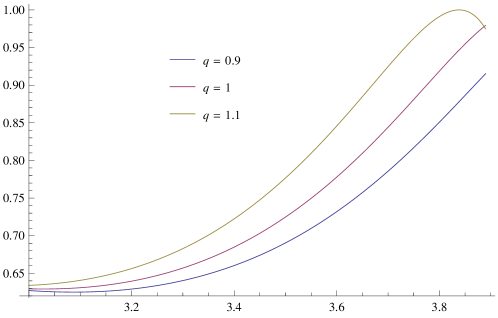
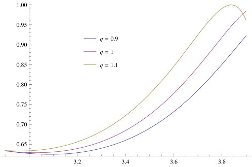
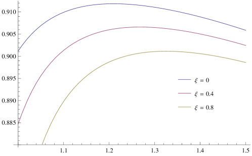
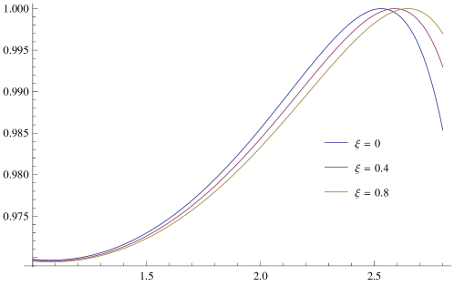
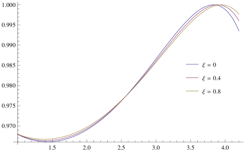
In the following plots we depict the greybody factor |Al|2superscriptsubscript𝐴𝑙2\left|A_{l}\right|^{2} as a function of ωrh𝜔subscript𝑟\omega r_{h}. In Fig. 3, we take Λ=0.001Λ0.001\Lambda=0.001, q=3.5𝑞3.5q=3.5, l=0𝑙0l=0, for different values of ξ𝜉\xi; in Fig. 4 Λ=0.05Λ0.05\Lambda=0.05, q=3.5𝑞3.5q=3.5, l=0𝑙0l=0, for different values of ξ𝜉\xi; in Fig. 5 Λ=0.01Λ0.01\Lambda=0.01, q=3.5𝑞3.5q=3.5 and l=0𝑙0l=0, for different values of ξ𝜉\xi; in Fig. 6 ξ=0.2𝜉0.2\xi=0.2, Λ=0.001Λ0.001\Lambda=0.001 and l=0𝑙0l=0, for different values of q𝑞q; in Fig. 7 ξ=1𝜉1\xi=1, Λ=0.001Λ0.001\Lambda=0.001, l=0𝑙0l=0, for different values of q𝑞q. An increase in value of the coupling parameter, decreases the greybody factor. This is due to the fact that non-minimal coupling plays the role of an effective mass and hence suppresses the greybody factor.
Refer to caption
Figure 3: Greybody factor as a function of ωrh𝜔subscript𝑟\omega r_{h} for different values of ξ𝜉\xi, when Λ=0.001Λ0.001\Lambda=0.001, q=3.5𝑞3.5q=3.5 and l=0𝑙0l=0.
Refer to caption
Figure 4: Greybody factor as a function of ωrh𝜔subscript𝑟\omega r_{h} for different values of ξ𝜉\xi , when Λ=0.05Λ0.05\Lambda=0.05, q=3.5𝑞3.5q=3.5 and l=0𝑙0l=0.
Refer to caption
Figure 5: Greybody factor as a function of ωrh𝜔subscript𝑟\omega r_{h} for different values of ξ𝜉\xi , when Λ=0.01Λ0.01\Lambda=0.01, q=3.5𝑞3.5q=3.5 and l=0𝑙0l=0.
Refer to caption
Figure 6: Greybody factor as a function of ωrh𝜔subscript𝑟\omega r_{h} for different values of q𝑞q, when ξ=0.2𝜉0.2\xi=0.2, Λ=0.001Λ0.001\Lambda=0.001 and l=0𝑙0l=0.
Refer to caption
Figure 7: Greybody factor as a function of ωrh𝜔subscript𝑟\omega r_{h} for different values of q𝑞q, when ξ=1𝜉1\xi=1, Λ=0.001Λ0.001\Lambda=0.001 and l=0𝑙0l=0.

3.5 Energy emission

The flux spectrum, that is, the number of massless scalar particles emitted by the black hole per unit time is given by LAE

dN(ω)dt=dω2π1eωTH1l=0(2l+1)Al(ω).𝑑𝑁𝜔𝑑𝑡𝑑𝜔2𝜋1superscript𝑒𝜔subscript𝑇𝐻1superscriptsubscript𝑙02𝑙1subscript𝐴𝑙𝜔\frac{dN\left(\omega\right)}{dt}=\frac{d\omega}{2\pi}\frac{1}{e^{\frac{\omega}{T_{H}}}-1}\sum_{l=0}^{\infty}\left(2l+1\right)A_{l}\left(\omega\right). (66)

By using the value from equation (65)65\left(\ref{57a}\right) into (66)66\left(\ref{58a}\right) we get

dN(ω)dt=dω2π1eωTH1l=0(2l+1)(1|ϝ2ϝ3ϝ1ϝ5ϝ1ϝ6ϝ2ϝ4|2).𝑑𝑁𝜔𝑑𝑡𝑑𝜔2𝜋1superscript𝑒𝜔subscript𝑇𝐻1superscriptsubscript𝑙02𝑙11superscriptsubscriptitalic-ϝ2subscriptitalic-ϝ3subscriptitalic-ϝ1subscriptitalic-ϝ5subscriptitalic-ϝ1subscriptitalic-ϝ6subscriptitalic-ϝ2subscriptitalic-ϝ42\frac{dN\left(\omega\right)}{dt}=\frac{d\omega}{2\pi}\frac{1}{e^{\frac{\omega}{T_{H}}}-1}\sum_{l=0}^{\infty}\left(2l+1\right)\sqrt{\left(1-\left|\frac{\digamma_{2}\digamma_{3}-\digamma_{1}\digamma_{5}}{\digamma_{1}\digamma_{6}-\digamma_{2}\digamma_{4}}\right|^{2}\right)}. (67)

Also, the differential energy rate is given by LAE

d2E(ω)dtdω=12πωeωTH1l=0(2l+1)Al(ω).superscript𝑑2𝐸𝜔𝑑𝑡𝑑𝜔12𝜋𝜔superscript𝑒𝜔subscript𝑇𝐻1superscriptsubscript𝑙02𝑙1subscript𝐴𝑙𝜔\frac{d^{2}E\left(\omega\right)}{dtd\omega}=\frac{1}{2\pi}\frac{\omega}{e^{\frac{\omega}{T_{H}}}-1}\sum_{l=0}^{\infty}\left(2l+1\right)A_{l}\left(\omega\right). (68)

On using the value of the greybody factor we get

d2E(ω)dtdω=12πωeωTH1l=0(2l+1)(1|ϝ2ϝ3ϝ1ϝ5ϝ1ϝ6ϝ2ϝ4|2).superscript𝑑2𝐸𝜔𝑑𝑡𝑑𝜔12𝜋𝜔superscript𝑒𝜔subscript𝑇𝐻1superscriptsubscript𝑙02𝑙11superscriptsubscriptitalic-ϝ2subscriptitalic-ϝ3subscriptitalic-ϝ1subscriptitalic-ϝ5subscriptitalic-ϝ1subscriptitalic-ϝ6subscriptitalic-ϝ2subscriptitalic-ϝ42\frac{d^{2}E\left(\omega\right)}{dtd\omega}=\frac{1}{2\pi}\frac{\omega}{e^{\frac{\omega}{T_{H}}}-1}\sum_{l=0}^{\infty}\left(2l+1\right)\sqrt{\left(1-\left|\frac{\digamma_{2}\digamma_{3}-\digamma_{1}\digamma_{5}}{\digamma_{1}\digamma_{6}-\digamma_{2}\digamma_{4}}\right|^{2}\right)}. (69)

The relevance of the low frequency limit is evident from the above results, that the coupling is only significant in this regime. As the coupling to scalar field is irrelevant in high frequency limits, the enhancement in emission rate occurs only at low frequencies.

3.6 Generalized absorption cross section

The definition of absorption cross section for asymptotically flat spacetimes is not valid for asymptotically non-flat spacetimes. For these cases the general formula for absorption cross section is given by LEG ; CBF

σ=l=0σl=πω2l=0(2l+1)Al(ω).𝜎superscriptsubscript𝑙0subscript𝜎𝑙𝜋superscript𝜔2superscriptsubscript𝑙02𝑙1subscript𝐴𝑙𝜔\sigma=\sum_{l=0}^{\infty}\sigma_{l}=\frac{\pi}{\omega^{2}}\sum_{l=0}^{\infty}\left(2l+1\right)A_{l}\left(\omega\right). (70)

Using the value from equation (65)65\left(\ref{57a}\right) we get

σ=l=0σl=πω2l=0(2l+1)(1|ϝ2ϝ3ϝ1ϝ5ϝ1ϝ6ϝ2ϝ4|2).𝜎superscriptsubscript𝑙0subscript𝜎𝑙𝜋superscript𝜔2superscriptsubscript𝑙02𝑙11superscriptsubscriptitalic-ϝ2subscriptitalic-ϝ3subscriptitalic-ϝ1subscriptitalic-ϝ5subscriptitalic-ϝ1subscriptitalic-ϝ6subscriptitalic-ϝ2subscriptitalic-ϝ42\sigma=\sum_{l=0}^{\infty}\sigma_{l}=\frac{\pi}{\omega^{2}}\sum_{l=0}^{\infty}\left(2l+1\right)\sqrt{\left(1-\left|\frac{\digamma_{2}\digamma_{3}-\digamma_{1}\digamma_{5}}{\digamma_{1}\digamma_{6}-\digamma_{2}\digamma_{4}}\right|^{2}\right)}.

4 Conclusion

In this paper, we have derived the analytic expression of greybody factor for non-minimally coupled scalar fields from Reissner-Nordström-de Sitter black hole in low energy approximation. This expression is valid for general partial modes. For coupling to scalar curvature, which can be regarded as mass or charge terms, greybody factor tend to zero like ω2superscript𝜔2\omega^{2}, irrespective of the values of the coupling parameter. A non-zero greybody factor in low frequency regime means that there is non-zero emission rate of Hawking radiations. The matching technique is used in deriving the formula for greybody factor. The significance of the results is elaborated by giving formulae for differential rate of energy and generalized absorption cross section from greybody factor.

The results of the present study reduce to those of Ref. PTN in appropriate limiting case, that is, if we put charge Q=0𝑄0Q=0 we recover the previously reported results. The effective potential and greybody factor are also analyzed graphically. We observe that the height of gravitational barrier increases with the increase of ξ𝜉\xi, the coupling parameter, whereas in the absence of this parameter it is decreased by increasing values of the cosmological constant. Also from the plot of greybody factor it is observed that an increase in the value of coupling parameter, decreases the greybody factor. This is due to the fact that non-minimal coupling plays the role of an effective mass and hence suppresses the greybody factor. Greybody factor is analyzed for different values of charge in the presence of non-minimal coupling.
Acknowledgement

KS acknowledges the support provided by the Center for the Fundamental Laws of Nature, Harvard University, during his visit while this work was underway. A research grant from the Higher Education Commission of Pakistan under its Project No. 20-2087 is gratefully acknowledged.

References

  • (1) S. Perlmutter et al., Astrophys. J. 517 (1999) 565.
  • (2) A. H. Guth, Phys. Rev. D 23 (1981) 347.
  • (3) N. Sanchez, Phys. Rev. D 18 (1978) 1030.
  • (4) C. Doran, A. Lasenby, S. Dolan and I. Hinder, Phys. Rev. D 71 (2002) 124020.
  • (5) S. Dolan, C. Doran and A. Lasenby, Phys. Rev. D 74 (2006) 064005.
  • (6) L. C. B. Crispino, S. R. Dolan and E. S. Oliveira, Phys. Rev. Lett 102 (2009) 231103.
  • (7) Y. S. Myung and H. W. Lee, Class. Quantum Grav. 20 (2003) 3533.
  • (8) S. Chen and J. Jing, Phys. Lett. B 691 (2010) 254.
  • (9) M. Liu, B. Yu, R. Wang and L. Xu, Mod. Phys. Lett. 25 (2010) 2431.
  • (10) J. M. Maldacena and A. Strominger, Phys. Rev. D 55 (1997) 861.
  • (11) S. S. Gubserv and I. R. Klebanov, Phys. Rev. Lett. 77 (1996) 4491.
  • (12) I. R. Klebanov and S. D. Mathur, Nucl. Phys. B 500 (1997) 115.
  • (13) M. Cvetic and F. Larsen, Phys. Rev. D 56 (1997) 4994.
  • (14) W. T. Kim and J. J. Oh, Phys. Lett. B 461 (1999) 189.
  • (15) J. Ahmed and K. Saifullah, Eur. Phys. J. C 77 (2017) 885.
  • (16) B. Carter, Phys. Rev. Lett. 33 (1974) 558.
  • (17) D. N. Page, Phys. Rev. D 14 (1976) 3260.
  • (18) W. G. Unruh, Phys. Rev. D 14 (1976) 3251.
  • (19) P. Kanti, J. Grain and A. Barrau, Phys. Rev. D 71 (2005) 104002.
  • (20) T. Harmark, J. Natario and R. Schiappa, Adv. Theor. Math. Phys 14 (2010) 727.
  • (21) L. C. B. Crispino, A. Higuchi, E. S. Oliveira and J. V. Rocha, Phys. Rev. D 87 (2013) 104034.
  • (22) P. Kanti, T. Pappas and N. Pappas, Phys. Rev. D 90 (2014) 124077.
  • (23) Z. Stuchlik and S. Hledík, Acta Physica Slovaca 52 (2002) 363.
  • (24) M. Abramowitz and I. Stegun, Handbook of Mathematical functions (Acedamic, New York, 1996).
  • (25) L. C. B. Crispino, E. S. Oliveira and G. E. A. Matsas, Phys. Rev. D 76 (2007) 107502.
  • (26) C. Cohen-Tannoudji, B. Diu and F. Laloe, Quantum Mechanics, Vol II John Wiley & Sons, New York (1977).