Minimum Sparsity of Unobservable
Power Network Attacks

Abstract

Physical security of power networks under power injection attacks that alter generation and loads is studied. The system operator employs Phasor Measurement Units (PMUs) for detecting such attacks, while attackers devise attacks that are unobservable by such PMU networks. It is shown that, given the PMU locations, the solution to finding the sparsest unobservable attacks has a simple form with probability one, namely, $\kappa(\mathcal{G^{M}})+1$, where $\kappa(\mathcal{G^{M}})$ is defined as the vulnerable vertex connectivity of an augmented graph. The constructive proof allows one to find the entire set of the sparsest unobservable attacks in polynomial time. Furthermore, a notion of the potential impact of unobservable attacks is introduced. With optimized PMU deployment, the sparsest unobservable attacks and their potential impact as functions of the number of PMUs are evaluated numerically for the IEEE 30, 57, 118 and 300-bus systems and the Polish 2383, 2737 and 3012-bus systems. It is observed that, as more PMUs are added, the maximum potential impact among all the sparsest unobservable attacks drops quickly until it reaches the minimum sparsity.

I Introduction

Modern power networks are increasingly dependent on information technology in order to achieve higher efficiency, flexibility and adaptability [1]. The development of more advanced sensing, communications and control capabilities for power grids enables better situational awareness and smarter control. However, security issues also arise as more complex information systems become prominent targets of cyber-physical attacks: not only can there be data attacks on measurements that disrupt situation awareness [2], but also control signals of power grid components including generation and loads can be hijacked, leading to immediate physical misbehavior of power systems [3]. Furthermore, in addition to hacking control messages, a powerful attacker can also implement physical attacks by directly intruding upon power grid components. Therefore, to achieve reliable and secure operation of a smart power grid, it is essential for the system operator to minimize (if not eliminate) the feasibility and impact of physical attacks.

There are many closely related techniques that can help achieve secure power systems. Firstly, coding and encryption can better secure control messages and communication links [4], and hence raise the level of difficulty of cyber attacks. To prevent physical attacks, grid hardening is another design choice [5]. However, grid hardening can be very costly, and hence may only apply to a small fraction of the components in large power systems. Secondly, power systems are subject to many kinds of faults and outages [6, 7, 8], which are in a sense unintentional physical attacks. As such outages are not inflicted by attackers, they are typically modeled as random events, and detecting outages is often modeled as a hypothesis testing problem [9]. However, this event and detection model is not necessarily accurate for intentional physical attacks, which are the focus of this paper. Indeed, an intelligent attacker would often like to strategically optimize its attack, such that it is not only hard to detect, but also the most viable to implement (e.g., with low execution complexity as well as high impact).

Recently, there has been considerable research concerning data injection attacks on sensor measurements from supervisory control and data acquisition (SCADA) systems. A common and important goal among these works is to pursue the integrity of network state estimation, that is, to successfully detect the injected data attack and recover the correct system states. The feasibility of constructing data injection attacks to pass bad data detection schemes and alter estimated system states was first shown in [2]. There, a natural question arises as to how to find the sparsest unobservable data injection attack, as sparsity is used to model the complexity of an attack, as well as the resources needed for an attacker to implement it. However, finding such an optimal attack requires solving an NP-hard $l_{0}$ minimization problem. While efficiently finding the sparsest unobservable attacks in general remains an open problem, interesting and exact solutions under some special problem settings have been developed in [10] [11] [12]. Another important aspect of a data injection attack is its impact on the power system. As state estimates are used to guide system and market operation of the grid, several interesting studies have investigated the impact of data attacks on optimal power flow recommendation [13] and location marginal prices in a deregulated power market [14] [15]. Furthermore, as Phasor Measurement Units (PMUs) become increasingly deployed in power systems, network situational awareness for grid operators is significantly improved compared to using legacy SCADA systems only. However, while PMUs provide accurate and secure sampling of the system states, their high installation costs prohibit ubiquitous deployment. Thus, the problem of how to economically deploy PMUs such that the state estimator can best detect data injection attacks is an interesting problem that many studies have addressed (see, e.g. [16, 17, 18] among others.)

Compared to data attacks that target state estimators, physical attacks that directly disrupt power network physical processes can have a much faster impact on power grids. In addition to physical attacks by hacking control signals or directly intruding upon grid components, several types of load altering attacks have been shown to be practically implementable via Internet-based message attacks [3]. Topological attacks are another type of physical attack which have been considered in [19]. Dynamic power injection attacks have also been analyzed in several studies. For example, in [20], conditions for the existence of undetectable and unidentifiable attacks were provided, and the sizes of the sets of such attacks were shown to be bounded by graph-theoretic quantities. Alternatively, in [21] and [22], state estimation is considered in the presence of both power injection attacks and data attacks. Specifically, in these works, the maximum number of attacked nodes that still results in correct estimation was characterized, and effective heuristics for state recovery under sparse attacks were provided.

In this paper, we investigate a specific type of physical attack in power systems called power injection attacks, that alter generation and loads in the network. A linearized power network model - the DC power flow model - is employed for simplifying the analysis of the problem and obtaining a simple solution that yields considerable insight. We consider a grid operator that employs PMUs to (partially) monitor the network for detecting power injection attacks. Since power injection attacks disrupt the power system states immediately, the timeliness of PMU measurement feedback is essential. Furthermore, our model allows for the power injections at some buses to be “unalterable”. This captures the cases of “zero injection buses” with no generation and load, and buses that are protected by the system operator. Under this model we study the open $l_{0}$ minimization problem of finding the sparsest unobservable attacks given any set of PMU locations. We start with a feasibility problem for unobservable attacks. We prove that the existence of an unobservable power injection attack restricted to any given set of buses can be determined with probability one by computing a quantity called the structural rank. Next, we prove that the NP-hard problem of finding the sparsest unobservable attacks has a simple solution with probability one. Specifically, the sparsity of the optimal solution is $\kappa(\mathcal{G^{M}})+1$, where $\kappa(\mathcal{G^{M}})$ is the “vulnerable vertex connectivity” that we define for an augmented graph of the original power network. Meanwhile, the entire set of globally optimal solutions (there can be many of them) is found in polynomial time. We further introduce a notion of potential impacts of unobservable attacks. Accordingly, among all the sparsest unobservable attacks, an attacker can easily find the one with the greatest potential impact. Finally, given optimized PMU placement, we evaluate the sparsest unobservable attacks in terms of their sparsity and potential impact in the IEEE 30, 57, 118 and 300-bus, and the Polish 2383, 2737 and 3012-bus systems.

The remainder of the paper is organized as follows. In Section II, models of the power network, power injection attacks, PMUs and unalterable buses are established. In addition, the minimum sparsity problem of unobservable attacks is formulated. In Section III we provide the feasibility condition for unobservable attacks restricted to any subset of the buses. In Section IV we prove that the minimum sparsity of unobservable attacks can be found in polynomial time with probability one. In Section V, a PMU placement algorithm for countering power injection attacks is developed, and numerical evaluation of the sparsest unobservable attacks in IEEE benchmark test cases and large-scale Polish power systems are provided. Conclusions are drawn in Section VI.

II Problem formulation

II-A Power network model

We consider a power network with $N$ buses, and denote the set of buses and the set of transmission lines by $\mathcal{N}=\{1,2,\ldots,N\}$ and $\mathcal{L}=\{1,2,\ldots,L\}$ respectively. For a line $\l\in\mathcal{L}$ that connects buses $n$ and $m$, denote its reactance by $x_{l}$ as well as $x_{nm}$, and define its incidence vector $\bm{m}_{l}$ as follows:

$$\bm{m}_{l}(i)=\left\{\begin{array}[]{lll}1,&\text{if }i=n,\\ -1,&\text{if }i=m,\\ 0,&\text{otherwise}.\end{array}\right.$$ (4)

Based on the power network topology and line reactances, we construct a weighted graph $\mathcal{G}=\{\mathcal{N},\mathcal{L},\bm{w}\}$ where the edge weight $w_{l}\triangleq\frac{1}{x_{l}},\forall l=1,\ldots,L$. The power system is generally modeled by nonlinear AC power flow equations [23]. In this paper, a linearized model - the DC power flow model - is employed as an approximation of the AC model, which allows us to find a simple closed-form solution to the problem from which we glean significant insights. Under the DC model, the real power injections $\bm{P}\in\mathbb{R}^{N}$ and the voltage phase angles $\bm{\theta}\in\mathbb{R}^{N}$ satisfy $\bm{P}=\bm{B}\bm{\theta}$, where $\bm{B}=\sum_{l=1}^{L}\frac{1}{x_{l}}\bm{m}_{l}\bm{m}_{l}^{T}\in\mathbb{R}^{N\times N}$ is the Laplacian of the weighted graph $\mathcal{G}$. We assume that $x_{l}$ is positive which is typically true for transmission lines (cf. Chapter 4 of [23]). Furthermore, the power flow on line $l$ from bus $n$ to bus $m$ equals $P_{nm}=\frac{1}{x_{nm}}(\theta_{n}-\theta_{m})$.

We consider attackers inflicting power injection attacks that alter the generation and loads in the power network. We denote the power injections in normal conditions by $\bm{P}$, and denote a power injection attack by $\Delta\bm{P}\in\mathbb{R}^{N}$. Thus the post-attack power injections are $\bm{P}+\Delta\bm{P}$.

II-B Sensor model and unobservable attacks

We consider the use of PMUs by the system operator for monitoring the power network in order to detect power injection attacks. With PMUs installed at the buses, we consider the following two different sensor models:

1. A PMU securely measures the voltage phasor of the bus at which it is installed.

2. A PMU securely measures the voltage phasor of the bus at which it is installed, as well as the current phasors on all the lines connected to this bus.

We denote the set of buses with PMUs by $\mathcal{M}~{}(\subseteq\mathcal{N})$, and let $M\triangleq|\mathcal{M}|$ be the total number of PMUs, where $|\cdot|$ denotes the cardinality of a set. Without loss of generality (WLOG), we choose one of the buses in $\mathcal{M}$ to be the angle reference bus. We say that a power injection attack $\Delta\bm{P}$ is unobservable if it leads to zero changes in all the quantities measured by the PMUs. With the first PMU model described above, we have the following definition:

Definition 1 (Unobservability condition).

An attack $\Delta\bm{P}\neq 0$ is unobservable if and only if

$$\exists\Delta\bm{\theta},~{}\text{such that}~{}\Delta\bm{P}=\bm{B}\Delta\bm{\theta}\text{ and }\Delta\bm{\theta}_{\mathcal{M}}=\bm{0},$$ (5)

where $\Delta\bm{\theta}_{\mathcal{\mathcal{M}}}$ denotes the $M\times 1$ sub-vector of $\Delta\bm{\theta}$ obtained by keeping its $M$ entries whose indices are in $\mathcal{M}$.

With the second PMU model described above, for any bus $n\in\mathcal{N}$, it is immediate to verify that the following three conditions are equivalent:

1. There are no changes of the voltage phasor at $n$ and of the current phasors on all the lines connected to $n$.

2. There are no changes of the voltage phasor at $n$ and of the power flows on all the lines connected to $n$.

3. $\forall n^{\prime}\in N[n]$, there is no change of the voltage phasor at $n^{\prime}$, where $N[n]$ is the closed neighborhood of $n$ which includes $n$ and its neighboring buses $N(n)$.

Thus, for forming unobservable attacks, the following two situations are equivalent to the attacker:

• The system operator monitors the set of buses $\mathcal{M}$ with the second PMU model;

• The system operator monitors the set of buses $N[\mathcal{M}]$ with the first PMU model,

where $N[\mathcal{M}]$ is the closed neighborhood of $\mathcal{M}$ which includes all the buses in $\mathcal{M}$ and their neighboring buses $N(\mathcal{M})$. Thus, the unobservability condition with the second PMU model is obtained by replacing $\mathcal{M}$ with $N[\mathcal{M}]$ in (5). WLOG, we employ the first PMU model in the following analysis, and based on the discussion above all the results can be directly translated to the second PMU model.

II-C Sparsest unobservable attacks

In forming an unobservable attack, an attacker generally has two objectives: minimize execution complexity and maximize its impact on the grid. Note that these two objectives can be competing interests that are not simultaneously achievable. We will first focus on finding the minimum execution complexity for an attack to be unobservable, which constitutes the main part of this work. Among attacks with the minimum complexity, we then find the one with the maximum impact.

For an attack vector $\Delta\bm{P}$, we use its zero norm $\|\Delta\bm{P}\|_{0}$ to model its execution complexity. This is because attackers are typically resource-constrained, and can choose only a limited number of buses to implement attacks. For minimizing attack complexity, an attacker is interested in finding the sparsest attacks that satisfy the unobservability condition (5):

$$\min_{\Delta\bm{\theta}}~{} \|\Delta\bm{P}\|_{0}$$ (6)

$$s.t.~{} \Delta\bm{P}=\bm{B\Delta\theta},~{}\Delta\bm{\theta}_{\mathcal{M}}=\bm{0},~{}\Delta\bm{\theta}\neq\bm{0}.$$

Since $\Delta\bm{\theta}_{\mathcal{M}}=\bm{0},~{}\Delta\bm{\theta}\neq\bm{0}\Rightarrow\bm{B\Delta\theta}=\bm{B}_{\mathcal{N}\mathcal{M}^{c}}\Delta\bm{\theta}_{\mathcal{M}^{c}},\Delta\bm{\theta}_{\mathcal{M}^{c}}\neq\bm{0}$, a more compact form of (6) is as follows:

$$\eqref{l0min}~{}\Leftrightarrow~{} \min_{\Delta\bm{\theta}_{\mathcal{M}^{c}}\neq\bm{0}}~{}\|\bm{B}_{\mathcal{N}\mathcal{M}^{c}}\Delta\bm{\theta}_{\mathcal{M}^{c}}\|_{0},$$ (7)

where $\mathcal{M}^{c}=\mathcal{N}\backslash\mathcal{M}$ denotes the complement of $M$, and $\bm{B}_{\mathcal{N}\mathcal{M}^{c}}$ is the submatrix of $\bm{B}$ formed by choosing all its rows and a set of columns $\mathcal{M}^{c}$.

We now note that problem (7) is NP-hard: Specifically, as a special case of the cospark problem of a matrix [24] problem (7) resembles a security index problem discussed in [12], which has been proven to be NP-hard. Under some special problem settings for data injection attacks, problems of this type have been shown to be solvable exactly in polynomial time [10] [11] [12]. In general, low complexity heuristics have been developed for solving $l_{0}$ minimization problems (e.g., $l_{1}$ relaxation).

We now generalize our model to allow a subset of buses to be “unalterable buses”, meaning that their nodal power injection cannot be changed by attackers. This allows us to model the following scenarios:

• A “zero injection” bus that simply connects multiple lines without nodal generation or load, and hence its power injection is always zero and cannot be changed.

• A “protected” bus by the system operator, and its power injection is not accessible by the attacker.

We denote the set of unalterable buses by $\mathcal{U}$. The other buses $\mathcal{U}^{c}$ are termed “alterable” buses. Generalizing (6), the sparsest unobservable attack problem is established as follows:

$$\min_{\Delta\bm{\theta}}~{} \|\Delta\bm{P}\|_{0}$$ (8)

$$s.t.~{} \Delta\bm{P}=\bm{B\Delta\theta},~{}\Delta\bm{\theta}_{\mathcal{M}}=\bm{0},~{}\Delta\bm{P}_{\mathcal{U}}=\bm{0},~{}\Delta\bm{\theta}\neq\bm{0}.$$

When $\mathcal{U}=\emptyset$, (8) reduces to (6). Generalizing (7), Eq. (8) has the following equivalent form:

$$\eqref{l0min_g}~{}\Leftrightarrow~{} \min_{\begin{subarray}{c}\Delta\bm{\theta}_{\mathcal{M}^{c}}\neq\bm{0},\\ \left(\bm{B}_{\mathcal{N}\mathcal{M}^{c}}\Delta\bm{\theta}_{\mathcal{M}^{c}}\right)_{\mathcal{U}}=0\end{subarray}}~{}\|\bm{B}_{\mathcal{N}\mathcal{M}^{c}}\Delta\bm{\theta}_{\mathcal{M}^{c}}\|_{0}.$$ (9)

II-D Graph augmentation

Given the locations of the sensors $\mathcal{M}$, we now introduce a variation of the graph $\mathcal{G}$ that will prove key to developing the main results later.

Definition 2.

Given a set of buses $\mathcal{M}\subseteq\mathcal{N}$, $\mathcal{G^{M}}$ is defined to be the following augmented graph based on $\mathcal{G}$:

1. $\mathcal{G^{M}}$ includes all the buses in $\mathcal{G}$, and has one additional unalterable dummy bus.

2. Define an augmented set $\bar{\mathcal{M}}$ that contains $\mathcal{M}$ and the unalterable dummy bus.

3. $\mathcal{G^{M}}$ includes all the edges of $\mathcal{G}$, and an edge is added between every pair of buses in $\bar{\mathcal{M}}$, and its weight can be chosen arbitrarily as any positive number.

We note that the dummy bus is only connected to the set of sensors $\mathcal{M}$. We observe the following key facts. First, an unobservable attack in the original graph $\mathcal{G}$ leads to zero changes in all the voltage phase angles in $\mathcal{M}$. Thus, any line between a pair of buses in $\mathcal{M}$ would see a zero change of the power flow on it. It is then clear that the added dummy bus and lines in $\mathcal{G^{M}}$ do not lead to any power flow changes in the network under any unobservable attack. We thus have the following lemma:

Lemma 1.

An attack is unobservable by $\mathcal{M}$ in $\mathcal{G}$ if and only if it is unobservable by $\mathcal{M}$ in $\mathcal{G^{M}}$.

This allows us to work with the augmented graph $\mathcal{G^{M}}$ instead of $\mathcal{G}$. It is clear that the weights of the added edges in $\mathcal{G^{M}}$ do not matter for Lemma 1 to hold.

III Feasibility condition of unobservable attacks

In this section, we address the following question whose solutions will be useful in solving the minimum sparsity problem (9): Assuming that the attacker can only alter the power injections at a subset of the buses, denoted by $\mathcal{A}\subseteq\mathcal{U}^{c}$, does there exist an attack that is unobservable by a set of PMUs $\mathcal{M}$? For any given $\mathcal{A}$, a feasible non-zero attack $\Delta\bm{P}~{}(\neq\bm{0})$ must satisfy $\Delta\bm{P}_{\mathcal{A}^{c}}=\bm{0}$. In other words, it must not alter the power injections at the buses in $\mathcal{A}^{c}$.

From (5), there exists an unobservable non-zero attack if and only if

$$\exists\Delta\bm{P},\Delta\bm{\theta}\neq\bm{0},~{}s.t.$$

$$~{}~{}~{}~{}\Delta\bm{P}=\bm{B}\Delta\bm{\theta},~{}\Delta\bm{P}_{\mathcal{A}^{c}}=\bm{0},~{}\Delta\bm{\theta}_{\mathcal{M}}=\bm{0}.$$ (10)

Since $\left\{\begin{array}[]{lll}\Delta\bm{\theta}_{\mathcal{M}}=\bm{0}\\ \Delta\bm{\theta}\neq\bm{0}\end{array}\right.\Rightarrow\Delta\bm{\theta}_{\mathcal{M}^{c}}\neq\bm{0},\Delta\bm{P}\neq\bm{0}$, we have that (10) is equivalent to

$$\exists\Delta\bm{\theta}_{\mathcal{M}^{c}}\neq\bm{0},~{}s.t.~{}(\Delta\bm{P}_{\mathcal{A}^{c}}=)~{}\bm{B}_{\mathcal{A}^{c}\mathcal{M}^{c}}\Delta\bm{\theta}_{\mathcal{M}^{c}}=\bm{0},$$ (11)

where $\bm{B}_{\mathcal{A}^{c}\mathcal{M}^{c}}$ is the submatrix of $\bm{B}$ formed by its rows $\mathcal{A}^{c}$ and columns $\mathcal{M}^{c}$. An illustration of (11) is depicted in Figure 1, where the submatrix formed by the shaded blocks represents $\bm{B}_{\mathcal{A}^{c}\mathcal{M}^{c}}$. From (11), we have the following lemma on the feasibility condition of unobservable attacks.

Lemma 2.

Given $\mathcal{A}$ and $\mathcal{M}$, there exists an unobservable non-zero attack if and only if $\bm{B}_{\mathcal{A}^{c}\mathcal{M}^{c}}$ is column rank deficient.

Figure 1: An illustration of (11) where the submatrix formed by the shaded blocks represents $\bm{B}_{\mathcal{A}^{c}\mathcal{M}^{c}}$.

To analyze when this column rank deficiency condition, $\operatorname{rank}\left(\bm{B}_{\mathcal{A}^{c}\mathcal{M}^{c}}\right)<|\mathcal{M}^{c}|$, is satisfied, we start with the following observations based on the fact that $\bm{B}$ is the Laplacian of the weighted graph $\mathcal{G}$.

1. The signs ($+1$, $-1$, or $0$) of the entries of $\bm{B}$ are fully determined by the network topology:

   $$\bm{B}_{ij}>0, \text{ if }i=j,$$

   $$\bm{B}_{ij}<0, i j~{}(i\neq j)$$ if node (bus) and node

   are $$\text{connected by an edge (transmission line)},$$

   $$\bm{B}_{ij}=0, i j~{}(i\neq j)$$ if node (bus) and node are

   not $$\text{connected}.$$

2. The values of the non-zero entries of $\bm{B}$ are determined by the line reactances $\{x_{ij}\}$:

   $$\bm{B}_{ii} =\sum_{j\neq i}w_{ij}=\sum_{j\neq i}\frac{1}{x_{ij}},$$

   $$\bm{B}_{ij} =-w_{ij}=-\frac{1}{x_{ij}},\text{ if }i\neq j\text{ and }\bm{B}_{ij}\neq 0.$$

When all the line reactances in the power network are known, so are the entries of the submatrix $\bm{B}_{\mathcal{A}^{c}\mathcal{M}^{c}}$, and it is immediate to compute whether $\operatorname{rank}\left(\bm{B}_{\mathcal{A}^{c}\mathcal{M}^{c}}\right)<|\mathcal{M}^{c}|$. Without knowing the exact values of any line reactances, we will show that whether $\operatorname{rank}\left(\bm{B}_{\mathcal{A}^{c}\mathcal{M}^{c}}\right)<|\mathcal{M}^{c}|$ can be determined almost surely by computing the structural rank of $\bm{B}_{\mathcal{A}^{c}\mathcal{M}^{c}}$, defined as follows [25].

Definition 3 (Set of independent entries).

A set of independent entries of a matrix $\bm{H}$ is a set of nonzero entries, no two of which lie on the same line (row or column).

Definition 4 (Structural rank).

The structural rank of a matrix $\bm{H}$, denoted by $\operatorname{sprank}(\bm{H})$, is the maximum number of elements contained in at least one set of independent entries.

A basic relation between the structural rank and the rank of a matrix is the following [25],

$$\operatorname{sprank}(\bm{B}_{\mathcal{A}^{c}\mathcal{M}^{c}})\geq\operatorname{rank}(\bm{B}_{\mathcal{A}^{c}\mathcal{M}^{c}}).$$ (12)

In the literature, structural rank is also termed “generic rank” [26].

Specifically, we consider generic power grid parameters, i.e., we assume that the line reactances $x_{l}~{}(l=1,2,\ldots,L)$ are independent, but not necessarily identical random variables drawn from continuous probability distributions. We assume that the reactances are bounded away from zero from below (as lines do not have zero reactances in practice). As such, the analysis in this work is along the line of structural properties as in [25] and [26], and we will develop results that hold with probability one. We believe the independence (but not identically distributed) assumption is sufficiently general in practice. In particular, there are uncertainties in factors that influence the reactance of a line (e.g. the distance that a line travels, the degradation of a line over time). These uncertainties can be modeled as independent (but not identically distributed) random variables, leading to the model employed in this paper.

Clearly, $\bm{B}_{\mathcal{A}^{c}\mathcal{M}^{c}}$ is always column rank deficient when $|\mathcal{A}^{c}|<|\mathcal{M}^{c}|$. Next, we discuss the case of $|\mathcal{A}^{c}|\geq|\mathcal{M}^{c}|$. We begin with the special case $\mathcal{A}=\mathcal{M}$, for which we have the following lemma whose proof is relegated to Appendix A:

Lemma 3.

Let $\bm{B}\in\mathbb{R}^{N\times N}$ be the Laplacian of a connected graph $\mathcal{G}$ with strictly positive edge weights. For any set of node indices $\mathcal{I}\subset\{1,2,\ldots,N\}$, denote by $\bm{B}_{\mathcal{II}}$ the submatrix of $\bm{B}$ formed by its rows $\mathcal{I}$ and columns $\mathcal{I}$. Then $\forall\mathcal{I},|\mathcal{I}|\leq N-1$, $\bm{B}_{\mathcal{II}}$ is of full rank.

Note that Lemma 3 holds deterministically without assuming generic edge weights of the graph. For the case of $\mathcal{A}=\mathcal{M}$, we let $\mathcal{I}=\mathcal{A}^{c}=\mathcal{M}^{c}$, and Lemma 3 proves that $\operatorname{rank}\left(\bm{B}_{\mathcal{A}^{c}\mathcal{M}^{c}}\right)=|\mathcal{M}^{c}|$. This implies the intuitive fact that there exists no attack restricted to $\mathcal{A}$ that is unobservable by a set of PMUs $\mathcal{M}=\mathcal{A}$.

Now, we address the general case of arbitrary $\mathcal{A}$ and $\mathcal{M}$. We have the following theorem demonstrating that having $\operatorname{sprank}(\bm{B}_{\mathcal{A}^{c}\mathcal{M}^{c}})=|\mathcal{M}^{c}|$ almost surely guarantees $\operatorname{rank}(\bm{B}_{\mathcal{A}^{c}\mathcal{M}^{c}})=|\mathcal{M}^{c}|$. The proof is relegated to Appendix B.

Theorem 1.

For a connected weighted graph $\mathcal{G}=\{\mathcal{N},\mathcal{L},\bm{w}\}$, assume that the edge weights are independent continuous random variables strictly bounded away from zero from below, and denote the Laplacian of $\mathcal{G}$ by $\bm{B}\in\mathbb{R}^{N\times N}$. Then, any $N^{\prime}\times N^{\prime\prime}$ submatrix of $\bm{B}$, with $\min(N^{\prime},N^{\prime\prime})\leq N-1$, has a rank of $\min(N^{\prime},N^{\prime\prime})$ with probability one if it has a structural rank of $\min(N^{\prime},N^{\prime\prime})$.

From Theorem 1, with $|\mathcal{A}^{c}|\geq|\mathcal{M}^{c}|$, if $\operatorname{sprank}(\bm{B}_{\mathcal{A}^{c}\mathcal{M}^{c}})=|\mathcal{M}^{c}|\leq N-1$, we have with probability one that $\operatorname{rank}(\bm{B}_{\mathcal{A}^{c}\mathcal{M}^{c}})=|\mathcal{M}^{c}|$, and there exists no attack restricted to $\mathcal{A}$ that is unobservable by a set of PMUs $\mathcal{M}$.

Remark 1.

It has been known in the literature that (see e.g., [25]), a full structural rank of a matrix leads to a full rank matrix with probability one, as long as the nonzero entries in the matrix are drawn independently from continuous probability distributions. However, it is worth noting that this is not sufficient for proving Theorem 1. This is because, as in Theorem 1, we are interested in matrices that are submatrices of a graph Laplacian: even with the edge weights of the graph drawn independently, the entries in these submatrices are correlated due to the special structure of a graph Laplacian. Such correlation leads to technical difficulties for the proof, which can be overcome as shown in Appendix B.

We note that the structural rank of a matrix can be computed in polynomial time by finding the maximum bipartite matching in a graph [25]. Since whether an entry of $\bm{B}$ is non-zero is solely determined by the topology of the network, we have the following corollary.

Corollary 1.

Given $\mathcal{A}$ and $\mathcal{M}$, whether a non-zero unobservable attack exists can be determined with probability one based solely on the knowledge of the grid topology.

IV Solving the sparsest unobservable attacks

In this section, we study the problem of finding the sparsest unobservable attacks given any set of PMUs $\mathcal{M}$ (cf. (9)). As remarked in Section II-C, $l_{0}$ minimization such as (9) is NP-hard. We will show that the sparsest unobservable attack can in fact be found in polynomial time with probability one. We first introduce a key concept — a vulnerable vertex cut. We then state our main theorem that yields an explicit solution for the sparsest unobservable attack problem (9). We prove that this solution both upper and lower bounds the optimum of (9), hence proving the theorem.

IV-A Vulnerable vertex cut and vulnerable vertex connectivity

We start with the following basic definitions:

Definition 5 (Vertex cut).

A vertex cut of a connected graph $\mathcal{G}$ is a set of vertices whose removal renders $\mathcal{G}$ disconnected.

Definition 6 (Vertex connectivity).

The vertex connectivity of a graph $\mathcal{G}$, denoted by $\kappa(\mathcal{G})$, is the size of the minimum vertex cut of $\mathcal{G}$, i.e., it is the minimum number of vertices that need to be removed to make the remaining graph disconnected.

From the definition of the augmented graph $\mathcal{G^{M}}$ in Section II-D, since all the buses in $\bar{\mathcal{M}}$ (containing $\mathcal{M}$ and the dummy bus) are pair-wise connected, we have the following lemma:

Lemma 4.

For any vertex cut of the augmented graph $\mathcal{G^{M}}$, there is no pair of the buses in $\bar{\mathcal{M}}$ that are disconnected by this cut.

Accordingly, we introduce the following notations which will be used later on:

Notation 1.

Given a vertex cut of $\mathcal{G^{M}}$, we denote the set of buses disconnected from $\bar{\mathcal{M}}$ after removing the cut set by $\mathcal{S}$. The cut set itself is denoted by $N(\mathcal{S})$.

With the vertex cut $N(\mathcal{S})$, $\mathcal{G^{M}}$ is partitioned into three subgraphs:

1. $\mathcal{S}$, which does not contain any bus in $\bar{\mathcal{M}}$, i.e., $\mathcal{S}\subseteq\bar{\mathcal{M}}^{c}$.

2. $N(\mathcal{S})$, which is the vertex cut set itself, and may contain buses in $\bar{\mathcal{M}}$.

3. $\mathcal{N}\backslash N[\mathcal{S}]$, which contains (not necessarily exclusively) all the remaining buses in $\bar{\mathcal{M}}$ after removing the cut set.

An illustrative example with a cut $N(\mathcal{S})$ of size 2 is depicted in Figure 2(b) in Section IV-C. We note that there is a slight abuse of notation in $N(S)$: In general, a cut set does not necessarily consist of exactly all the neighboring nodes of $S$. Nonetheless, as will be shown in the remainder of the paper, we need only care about the minimum cut set, which indeed consists of exactly all the neighboring nodes of $S$, namely, $N(S)$. Leveraging the above notation, we now introduce a key type of vertex cut on $\mathcal{G^{M}}$.

Definition 7 (Vulnerable vertex cut).

A vulnerable vertex cut of a connected augmented graph $\mathcal{G^{M}}$ is a vertex cut $N(\mathcal{S})$ for which $|\mathcal{U}^{c}\cap N[\mathcal{S}]|\geq|N(\mathcal{S})|+1$.

In other words, the number of alterable buses in $N[\mathcal{S}]$ is no less than the cut size plus one. The reason for calling such a vertex cut “vulnerable” will be made exact later in Section IV-C. The basic intuition is the following. In order to have $\Delta\bm{\theta}_{\mathcal{M}}=0$ (unobservability), the key is to have the phase angle changes on the cut $N(\mathcal{S})$ be zero, with power injection changes (which can only happen on the alterable buses) restricted in $N[\mathcal{S}]$. As will be shown later, this can be achieved if a cut $N(\mathcal{S})$ is “vulnerable” as defined above. We note that it is possible that no vulnerable vertex cut exists (e.g., in the extreme case that all buses are unalterable).

Accordingly, we define the following variation on the vertex connectivity.

Definition 8 (Vulnerable vertex connectivity).

The vulnerable vertex connectivity of an augmented graph $\mathcal{G^{M}}$, denoted by $\bar{\kappa}(\mathcal{G^{M}})$, is the size of the minimum vulnerable vertex cut of $\mathcal{G^{M}}$. If no vulnerable vertex cut exists, $\bar{\kappa}(\mathcal{G^{M}})$ is defined to be $\infty$.

We note that the concepts of vulnerable vertex cut and vulnerable vertex connectivity do not apply to the original graph $\mathcal{G}$. We immediately have the following lemma:

Lemma 5.

If a vulnerable vertex cut exists, then $\bar{\kappa}(\mathcal{G^{M}})\leq M=|\mathcal{M}|$.

Proof.

Suppose a vulnerable vertex cut exists, and $\bar{\kappa}(\mathcal{G^{M}})\geq M+1$. Denote the minimum vulnerable vertex cut by $N(\mathcal{S})$ (cf. Notation 1). Now consider the set $\mathcal{M}$: it is a vertex cut of $\mathcal{G^{M}}$ that separates the dummy bus and $\bar{\mathcal{M}}^{c}$. Because there are at least $\bar{\kappa}(\mathcal{G^{M}})+1\geq M+2$ alterable buses in $N[\mathcal{S}]\subseteq N[\bar{M}^{c}]$, $\mathcal{M}$ is also a vulnerable vertex cut. This contradicts the minimum vulnerable vertex cut having size at least $M+1$. ∎

IV-B Main result

We now state the following theorem that gives an explicit solution of the sparsest unobservable attack problem in terms of the vulnerable vertex connectivity $\bar{\kappa}(\mathcal{G^{M}})$.

Theorem 2.

For a connected grid $\mathcal{G=\{N,L},\bm{w}\}$, assume that the line reactances $x_{l}~{}(l\in\mathcal{L})$ are independent continuous random variables strictly bounded away from zero from below. Given any $\mathcal{M}$ and $\mathcal{U}$, the minimum sparsity of unobservable attacks, i.e., the global optimum of (9), equals $\bar{\kappa}(\mathcal{G^{M}})+1$ with probability one.

We note that finding the minimum vulnerable vertex connectivity of a graph is computationally efficient. For polynomial time algorithms we refer the readers to [27] and [28]. In particular, vertex cuts are enumerated [28] starting from the minimum and with increasing sizes, until a minimum vulnerable vertex cut is identified. We now prove Theorem 2 by upper and lower bounding the minimum sparsity of unobservable attacks in the following two subsections.

IV-C Upper bounding the minimum sparsity of unobservable attacks

We show that any vulnerable vertex cut $N(\mathcal{S})$ provides an upper bound on the optimum of (9) as follows.

Theorem 3.

For a connected grid $\mathcal{G}$ and a set of PMUs $\mathcal{M}$, for any vulnerable vertex cut of $\mathcal{G^{M}}$ denoted by $N(\mathcal{S})$ (cf. Notation 1), there exists an unobservable attack of sparsity no higher than $|N(\mathcal{S})|+1$.

Proof.

A vulnerable vertex cut $N(\mathcal{S})$ partitions $\mathcal{G^{M}}$ into $\mathcal{S}$, $N(\mathcal{S})$ and $\mathcal{N}\backslash\mathcal{N[S]}$, with $\mathcal{S}\subseteq\mathcal{M}^{c}$. Similarly to the range space interpretation of the sparsest unobservable attack (9), it is sufficient to show that there exists a non-zero vector in the range space of $\bm{B}_{\mathcal{N}\mathcal{S}}$ such that i) it has a sparsity no higher than $|N(\mathcal{S})|+1$, and ii) non-zero power injections occur only at the alterable buses.

By re-indexing the buses, WLOG, i) let $\mathcal{S}=\{1,2,\ldots,|\mathcal{S}|\}$, and ii) let $\bm{B}_{\mathcal{N}\mathcal{S}}$ have the following partition as depicted in Figure 2(a):

1. The top submatrix $\bm{B}_{\mathcal{S}\mathcal{S}}$ is an $|\mathcal{S}|\times|\mathcal{S}|$ matrix.

2. The middle submatrix (which will be shown to be $\bm{B}_{N(\mathcal{S})\mathcal{S}}$) consists of all the remaining rows, each of which has at least one non-zero entry.

3. The bottom submatrix is an all-zero matrix.

In particular, from the definition of the Laplacian, the middle submatrix of $\bm{B}_{\mathcal{N}\mathcal{S}}$, as described above, is exactly $\bm{B}_{N(\mathcal{S})\mathcal{S}}$ because its row indices correspond to those buses not in $\mathcal{S}$ but connected to at least one bus in $\mathcal{S}$.

From the definition of the vulnerable vertex cut, $|\mathcal{U}^{c}\cap N[\mathcal{S}]|\geq|N(\mathcal{S})|+1$. Now, pick any set of $|N(\mathcal{S})|+1$ alterable buses in $\mathcal{U}^{c}\cap N[\mathcal{S}]$, denote this set by $\mathcal{A}$, and denote the other buses in $N[\mathcal{S}]$ by $\tilde{U}\triangleq N[\mathcal{S}]\backslash\mathcal{A}$. Clearly, $|\tilde{U}|=|S|-1$. Therefore, $\bm{B}_{\tilde{\mathcal{U}}\mathcal{S}}$ (which is a submatrix of $\bm{B}_{N[\mathcal{S}]\mathcal{S}}$) has $|S|$ columns but only $|S|-1$ rows, and is hence column rank deficient.

Now, we let $\Delta\bm{\theta}_{\mathcal{S}}$ be a non-zero vector in the null space of $\bm{B}_{\tilde{\mathcal{U}}\mathcal{S}}$:

$$\bm{B}_{\tilde{\mathcal{U}}\mathcal{S}}\Delta\bm{\theta}_{\mathcal{S}}=\bm{0}.$$ (13)

Then, we construct an attack vector $\Delta\bm{P}=\bm{B}_{\mathcal{N}\mathcal{S}}\Delta\bm{\theta}_{\mathcal{S}}$: it has some possibly non-zero values at the indices that correspond to $\mathcal{A}$, and has zero values at all other indices. Thus,

$$\|\Delta\bm{P}\|_{0}\leq|\mathcal{A}|=|N(\mathcal{S})|+1.$$ (14)

∎

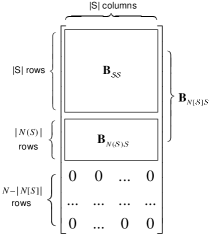
(a) Block representation of $\bm{B}_{\mathcal{N}\mathcal{S}}$.

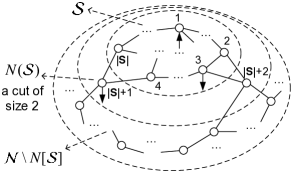
(b) A 3-sparse unobservable power injection attack.

Figure 2: Sparse attacks with voltage phase angle changes restricted to buses $1,2,\ldots|\mathcal{S}|$.

Theorem 3 explains our terminology of a “vulnerable vertex cut”, since if a vertex cut is vulnerable, it leads to an unobservable attack. If a vulnerable vertex cut of $\mathcal{G^{M}}$ exists, applying Theorem 3 to the minimum one, we have that the optimum of (9) is upper bounded by $\bar{\kappa}(\mathcal{G^{M}})+1$. If no vulnerable vertex cut exists, $\bar{\kappa}(\mathcal{G^{M}})+1=\infty$ is a trivial upper bound.

We now provide a graph-theoretic interpretation of Theorem 3. As shown in Figure 2(a) and 2(b), all the buses can be partitioned into three subsets $\mathcal{S},N(\mathcal{S})$ and $\mathcal{N}\backslash N[\mathcal{S}]$, corresponding to the row indices of the top, middle and bottom submatrices of $\bm{B}_{\mathcal{N}\mathcal{S}}$, respectively. $N(\mathcal{S})$ is a vulnerable vertex cut of $\mathcal{G^{M}}$ that separates $\mathcal{S}$ from $\mathcal{N}\backslash N[\mathcal{S}]$. The sparse attack $\Delta\bm{P}$ (cf. (14)) is formed by injecting/extracting power at $|N(\mathcal{S})|+1$ alterable buses in $N[\mathcal{S}]$, such that the phase angle changes at $\mathcal{N}\backslash\mathcal{S}$ are all zero. Note that $(\mathcal{N}\backslash\mathcal{S})\supseteq\mathcal{M}$. The example with $|N(\mathcal{S})|=2$ in Figure 2(b) illustrates a $3$-sparse attack with power injection/extractions at (assumed alterable) buses $1,3$ and $|\mathcal{S}|+1$, such that the phase angle changes at $\mathcal{N}\backslash\mathcal{S}$ are all zero.

We end this subsection by introducing a notion of “potential impact” of unobservable attacks. We make the following observation: As long as an attacker takes control of all the power injections in a vulnerable vertex cut $N(\mathcal{S})$ (assuming they are alterable), it can always cancel out the effects of anything that happens within $N[\mathcal{S}]$ on the measurements taken in $\mathcal{M}~{}(\subseteq\mathcal{N}\backslash\mathcal{S})$. Thus, by taking control of all the buses in $N(\mathcal{S})$, an attacker can successfully hide from the system operator a power injection attack with a zero norm as large as

$$|N[\mathcal{S}]|=|N(\mathcal{S})|+|\mathcal{S}|~{}(\gg|N(\mathcal{S})|+1).$$ (15)

Accordingly, we introduce the following definition.

Definition 9.

The potential impact of unobservable attacks associated with a vulnerable vertex cut $N(\mathcal{S})$ is defined as $|N[\mathcal{S}]|$.

Remark 2.

Definition 9 is one characterization of attack impact based solely on graph theoretic properties. In practice, there are many different notions of attack impact depending on, e.g., the interpretation of the attacks and the operating objective of the system.

Employing Definition 9, we can differentiate the potential impacts of multiple sparsest unobservable attacks with the same sparsity. An illustration is depicted in Figure 3. In this example, two vulnerable vertex cuts both of size two, $N(\mathcal{S}_{1})=\{V_{1A},V_{1B}\}$ and $N(\mathcal{S}_{2})=\{V_{2A},V_{2B}\}$, are enclosed by solid ovals. Accordingly, both cuts enable 3-sparse unobservable attacks. However, their potential impacts are significantly different. Cut $N(\mathcal{S}_{2})$ only disconnects one other bus, namely $\mathcal{S}_{2}=\{V_{2C}\}$ from the set of PMUs $\mathcal{M}$, and hence its potential impact equals $|N[\mathcal{S}_{2}]|=3$. In comparison, cut $N(\mathcal{S}_{1})$ disconnects all the vertices above $N(\mathcal{S}_{1})$ from $\mathcal{M}$, and hence its potential impact equals $|N[\mathcal{S}_{1}]|\gg 3$. With this definition of potential impact, it is then natural for an attacker to seek the sparsest unobservable attack with the greatest potential impact.

As an immediate byproduct of the analysis of potential impact, by letting $\mathcal{S}=\mathcal{M}^{c}$, we obtain the maximum potential impact of all unobservable attacks in a power network:

Corollary 2.

For a connected power grid $\mathcal{G=\{N,L},\bm{w}\}$, given any $\mathcal{M}$ denoting the PMU locations, the maximum potential impact among all the unobservable attacks equals $|N[\mathcal{M}^{c}]|$.

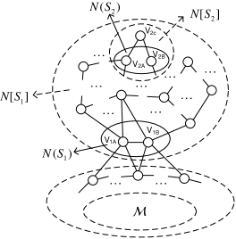
Figure 3: An illustration of two vulnerable vertex cuts with the same size but different potential impacts.

IV-D Lower bounding the sparsity of unobservable attacks

We first define the following property of a matrix $\bm{H}\in\mathbb{R}^{N\times N}$, which will be shown to be equivalent to having $\operatorname{sprank}(\bm{H})=N$.

Property 1 (An equivalent condition for having a full structural rank).

$$\forall n=1,2,\ldots,N,\text{ and for any }n\times N\text{ submatrix of }\bm{H},$$

the submatrix has at least $$n$$ columns each with at least

one non-zero entry.

We have the following lemma whose proof is relegated to Appendix C:

Lemma 6.

Property 1 is equivalent to having $\operatorname{sprank}(\bm{H})=N$.

We now prove the lower bounding part of Theorem 2, namely, with probability one, all unobservable power injection attacks $\Delta\bm{P}$ must have $\|\Delta\bm{P}\|_{0}\geq\bar{\kappa}(\mathcal{G^{M}})+1$. The key idea is in showing that the equivalence between Property 1 and a full structural rank (cf. Lemma 6) implies a connection between the vulnerable vertex connectivity and the feasibility condition of unobservable attacks (cf. Lemma 2).

Proof of $\|\Delta\bm{P}\|_{0}\geq\bar{\kappa}(\mathcal{G^{M}})+1$ for unobservable $\Delta\bm{P}$, w.p.1.

We focus on $\mathcal{G^{M}}$ and consider its corresponding Laplacian $\bm{B}$. Suppose there exists a power injection attack $\Delta\bm{P}\neq\bm{0}$ such that

$$\Delta\bm{\theta}_{\mathcal{M}}=\bm{0}\text{ and }\|\Delta\bm{P}\|_{0}\leq{\bar{\kappa}(\mathcal{G^{M}})}.$$ (16)

Denote the buses with non-zero power injection changes by $\mathcal{A}\subseteq\mathcal{U}^{c}$, and hence $\Delta\bm{P}_{\mathcal{A}^{c}}=\bm{0}$. From (16), $|\mathcal{A}|\leq\bar{\kappa}(\mathcal{G^{M}}),\Delta\bm{\theta}_{\mathcal{M}^{c}}\!\neq\!\bm{0}$, and $\bm{0}\!=\!\Delta\bm{P}_{\mathcal{A}^{c}}\!=\!\bm{B}_{\mathcal{A}^{c}\mathcal{M}^{c}}\Delta\bm{\theta}_{\mathcal{M}^{c}}$, implying that $\bm{B}_{\mathcal{A}^{c}\mathcal{M}^{c}}$ is column rank deficient. We first consider the case that a vulnerable vertex cut exists, i.e., $\bar{\kappa}(\mathcal{G^{M}})<\infty$. The proof for the case of $\bar{\kappa}(\mathcal{G^{M}})=\infty$ follows similarly. For notational simplicity, we will use $\bar{\kappa}$ instead of $\bar{\kappa}(\mathcal{G^{M}})$ in the remainder of the proof.

If a vulnerable vertex cut exists, i.e., $\bar{\kappa}<\infty$

We will prove that, for all $\mathcal{A}\subseteq\mathcal{U}^{c}$ with $|\mathcal{A}|\leq\bar{\kappa}$, $\bm{B}_{\mathcal{A}^{c}\mathcal{M}^{c}}$ is of full column rank with probability one, i.e., (16) can only happen with probability zero. From Lemma 5, $\bar{\kappa}\leq M$. It is then sufficient to prove for the “worst cases” with $|\mathcal{A}|=\bar{\kappa}=M$, i.e., $|\mathcal{A}^{c}|=|\mathcal{M}^{c}|=N-\bar{\kappa}$ and $\bm{B}_{\mathcal{A}^{c}\mathcal{M}^{c}}$ is a square matrix. From Theorem 1 and Lemma 6, it is sufficient to show that $\bm{B}_{\mathcal{A}^{c}\mathcal{M}^{c}}$ satisfies Property 1, and hence is of full rank with probability one. Recall from the definition of the Laplacian $\bm{B}$ that, for any column (or row) of $\bm{B}$, $\bm{b}_{i},(i=1,\ldots,N)$, its non-zero entries correspond to bus $i$ and those buses that are connected to bus $i$. With this, we now prove that $\bm{B}_{\mathcal{A}^{c}\mathcal{M}^{c}}$ satisfies Property 1.

Consider any set of $n$ ($\leq N-\bar{\kappa}$) buses in $\mathcal{A}^{c}$, denoted by $\tilde{\mathcal{N}}$.

i) If $\tilde{\mathcal{N}}\subseteq\mathcal{M}^{c}$: Based on the definition of the Laplacian $\bm{B}$, the $n$ columns of $\bm{B}_{\tilde{\mathcal{N}}\mathcal{M}^{c}}$ that correspond to the buses $\tilde{\mathcal{N}}$ themselves each has at least one non-zero entry.

ii) If $\tilde{\mathcal{N}}\cap\mathcal{M}\neq\emptyset$: We prove that $N(\tilde{\mathcal{N}})$ must contain at least $\bar{\kappa}$ buses. This is because, otherwise, $|N(\tilde{\mathcal{N}})|\leq\bar{\kappa}-1$, contradicting that $\bar{\kappa}$ is the minimum size of vulnerable vertex cuts for the following reasons:

1. $\mathcal{A}\subseteq\tilde{\mathcal{N}}^{c}$, and thus $\tilde{\mathcal{N}}^{c}$ has at least $|\mathcal{A}|=\bar{\kappa}$ alterable buses.

2. $|N(\tilde{\mathcal{N}})|\leq\bar{\kappa}-1$ implies that $\tilde{\mathcal{N}}^{c}\backslash N(\tilde{\mathcal{N}})\neq\emptyset$, and thus $N(\tilde{\mathcal{N}})$ is a vertex cut that separates $\tilde{\mathcal{N}}$ and $\tilde{\mathcal{N}}^{c}\backslash N(\tilde{\mathcal{N}})$.

3. Because $\tilde{\mathcal{N}}\cap\mathcal{M}\neq\emptyset$ and $\mathcal{M}$ are pairwise connected in $\mathcal{G^{M}}$, $\mathcal{M}\subseteq N[\tilde{\mathcal{N}}]$. Thus, $\tilde{\mathcal{N}}^{c}\backslash N(\tilde{\mathcal{N}})$ and $\mathcal{M}$ are disjoint.

From 1), 3), and the fact that $|N(\tilde{\mathcal{N}})|\leq\bar{\kappa}-1$, we observe that $N(\tilde{\mathcal{N}})$ is a vulnerable vertex cut of size $\bar{\kappa}-1$, contradicting $\bar{\kappa}$ being the vulnerable vertex connectivity.

Now, based on the definition of the Laplacian $\bm{B}$, the $n\times N$ submatrix $\bm{B}_{\tilde{\mathcal{N}}\mathcal{N}}$ must have at least $n+\bar{\kappa}$ columns each of which has at least one non-zero entry for the following reasons:

• The $n$ columns of $\bm{B}_{\tilde{\mathcal{N}}\mathcal{N}}$ that correspond to the buses $\tilde{\mathcal{N}}$ themselves each has at least one non-zero entry.

• As $\tilde{\mathcal{N}}$ are connected to at least $\bar{\kappa}$ other buses, each one of these $\bar{\kappa}$ neighbors of $\tilde{\mathcal{N}}$ corresponds to one column of $\bm{B}_{\tilde{\mathcal{N}}\mathcal{N}}$ that has at least one non-zero entry.

Accordingly, the $n\times(N-{\bar{\kappa}})$ submatrix $\bm{B}_{\tilde{\mathcal{N}}\mathcal{M}^{c}}$ has at least $n$ columns each of which has at least one non-zero entry.

Summarizing i) and ii), $\bm{B}_{\mathcal{A}^{c}\mathcal{M}^{c}}$ satisfies Property 1, and is thus of full column rank with probability one. Therefore, (16) can only happen with probability zero.

If no vulnerable vertex cut exists, i.e., $\bar{\kappa}=\infty$

If $\mathcal{M}=\mathcal{N}$, i.e., all buses have PMUs, then clearly no unobservable attack exists. We now focus on $M\leq N-1$. Suppose $|\mathcal{A}|\geq M+1$. Consider the set $\bar{M}$ containing $\mathcal{M}$ and the dummy bus. $\Delta\bm{\theta}_{\mathcal{M}}=\bm{0}$ (cf. (16)) implies that $\mathcal{A}\subseteq N[\bar{\mathcal{M}}^{c}]$, and thus $N[\bar{\mathcal{M}}^{c}]$ has at least $|\mathcal{A}|\geq M+1$ alterable buses. Since $\mathcal{M}~{}(=N(\bar{\mathcal{M}}^{c}))$ separates the dummy node and $\mathcal{N}\backslash\mathcal{M}$, $\mathcal{M}$ is a vulnerable vertex cut. This contradicts the nonexistence of a vulnerable vertex cut. Therefore, $|\mathcal{A}|\leq M$. In this case, the same proof as in the above case i) when a vulnerable vertex cut exists applies, and (16) can only happen with probability zero. ∎

With the proofs of upper and lower bounds, we have now proved Theorem 2. In addition, from the proof of Theorem 3, we have a constructive solution of the sparsest unobservable attack in polynomial time. We conclude this section by noting the following fact similar to that in Section III: the minimum sparsity of unobservable attacks is fully determined with probability one by the network topology, the locations of the alterable buses, and the locations of the PMUs.

TABLE I: Algorithm 1

Greedy algorithm for PMU placement for countering power injection attacks
Place the $1^{st}$ PMU at bus 1.
Repeat
	If no unobservable attack exists given the current set of PMUs $\mathcal{M}$, stop.
	Step 1: Find all the minimum vulnerable vertex cuts of $\mathcal{G}^{N[\mathcal{M}]}$;
	among them, find the cut with the greatest potential impact,
	denoted by $C(\mathcal{G}^{N[\mathcal{M}]})$.
	Step 2: Among all the buses disconnected from $N[\mathcal{M}]$ by $C(\mathcal{G}^{N[\mathcal{M}]})$
	as well as those in the cut set $C(\mathcal{G}^{N[\mathcal{M}]})$, place the next PMU
	at the one such that the resulting maximum potential impact
	among all the remaining unobservable attacks is minimized.

V Numerical evaluation

In this section, we evaluate the sparsest unobservable attacks and their potential impacts when the system operator deploys PMUs at optimized locations. We first provide an efficient algorithm for optimizing PMU placement by the system operator. Next, we provide comprehensive evaluation of our analysis and algorithms in multiple IEEE power system test cases as well as large-scale Polish power systems. Our MATLAB codes are openly available for download.

V-A Optimization of PMU placement for attack detection

We have seen in Section IV that the minimum sparsity and potential impacts of unobservable attacks are determined fully by the network topology, the locations of the alterable buses, and the PMU placement. Note that, unlike network states and parameters which can vary over short and medium time scales, the transmission network topology and the alterable buses typically stay the same over relatively long time scales. This motivates the system operator to optimize the PMU placement according to this information.

For the best performance in countering power injection attacks, the system operator wants to raise the minimum sparsity of unobservable attacks, as well as mitigate the maximum potential impact of unobservable attacks. Algorithm 1 (cf. Table I) is developed for the system operator to greedily place PMUs to pursue both objectives. In this algorithm, we have assumed that the second PMU model in Section II-B is employed, and the algorithm can be adapted to the first PMU model by replacing $N[\mathcal{M}]$ with $\mathcal{M}$.

Algorithm 1 is essentially a successive cut/attack elimination procedure. The purpose of Step 1 is to identify the sparsest unobservable attack with the greatest potential impact. Specifically, Step 1 can be performed as follows:

1. Assign arbitrarily one of the buses in $\mathcal{M}$ as the source node;

2. For each of the buses in $\mathcal{N}\backslash N[\mathcal{M}]$, assign it as the destination node, and compute all the minimum vulnerable vertex cuts that separate such a source-destination pair.

3. Among all the computed source-destination vertex cuts that have the same minimum size, compute their corresponding potential impacts, and select the minimum vertex cut with the greatest potential impact, denoted by $C(\mathcal{G}^{N[\mathcal{M}]})$.

We note that all the minimum vulnerable vertex cuts can be enumerated in polynomial time (c.f. [28]). In our numerical evaluation using MATLAB on a laptop with Intel Core i7 3.1-GHz CPU and 8 GB of RAM, it takes less than $0.2$ seconds on average for every PMU placed for the IEEE 300 bus systems. This per-PMU time increases to about 50 seconds for the Polish 3012 bus system. In Step 2, our primary goal is to ensure that the cut set $C(\mathcal{G}^{N[\mathcal{M}]})$ found in Step 1 does not remain a legitimate vertex cut after placing the next PMU. This can be achieved by placing the next PMU among the buses disconnected from $N[\mathcal{M}]$ by $C(\mathcal{G}^{N[\mathcal{M}]})$ as well as those in $C(\mathcal{G}^{N[\mathcal{M}]})$. Among such candidate buses, we choose the one that renders the minimum maximum potential impact among all the remaining unobservable attacks (cf. Corollary 2) had the next PMU been placed at it.

V-B Numerical evaluation of unobservable attacks vs. number of PMUs

We evaluate our results in the IEEE 30-bus, IEEE 57-bus, IEEE 118-bus, IEEE 300-bus, Polish 2383-bus, Polish 2737-bus, and Polish 3012-bus systems. The evaluation is performed based on the software toolbox MATPOWER [29]. In each of these systems, we apply Algorithm 1 to generate a set of PMU locations greedily, with the number of PMUs $M$ increasing from one until all attacks become observable. Moreover, from Algorithm 1, for all $M$, the minimum sparsity of unobservable attacks as well as the maximum potential impact among the sparsest unobservable attacks are found (cf. Step 1 in Algorithm 1). We assume that all buses are alterable in the test cases.

In general, for a given set of PMUs, one can also search for the maximum potential impact among all $s$-sparse unobservable attacks for any given sparsity $s$, (as opposed to evaluate that among the sparsest attacks only as in Algorithm 1). However, this problem is NP-hard in $s$. In light of this, we selectively focused on some level of sparsity of unobservable attacks that is not minimally sparse, and evaluated their maximum potential impacts.

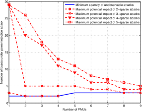
Figure 4: Minimum sparsity of unobservable attacks and maximum potential impacts of 2, 3, 4, 5-sparse attacks as functions of $M$, IEEE 30-bus system.

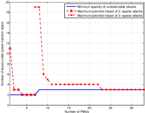
Figure 5: Minimum sparsity of unobservable attacks and the maximum potential impacts of the sparsest attacks as functions of $M$, IEEE 118-bus system.

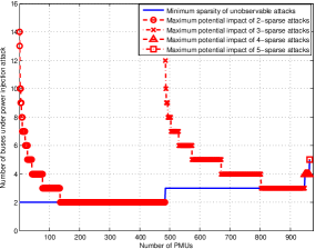
Figure 6: Minimum sparsity of unobservable attacks and the maximum potential impacts of the sparsest attacks as functions of $M$, Polish 3012-bus system.

Specifically, the minimum sparsity of unobservable attacks and the maximum potential impact among these sparsest attacks both as functions of the number of PMUs $M$ are plotted for the IEEE 30 and 118-bus power systems and the Polish 3012-bus system, in Figures 4, 5 and 6 respectively. In addition,

• For the IEEE 30-bus system, the maximum potential impact among all 2-sparse, 3-sparse, 4-sparse and 5-sparse unobservable attacks for the entire range of $M$ are plotted. (Note that the minimum sparsity of unobservable attacks does not exceed 3 for all $M$).

• For the IEEE 118-bus system, the maximum potential impact among all 3-sparse attacks when $M\geq 7$ is plotted. (Note that for $M=7$ the minimum sparsity of unobservable attacks is 2).

We make the following observations which appear in all seven of the evaluated systems:

• In all seven systems, all the attacks become observable with less than a third of the buses installed with PMUs (assuming the second PMU model). The average percentage of the number of PMUs needed to have full network observability equals $31.1\%$. While this number resembles a well-known estimate of such percentage to be one third [30], it also demonstrates the efficacy of Algorithm 1 in PMU placement.

• The topologies of the tested power systems tend to allow sparse power injection attacks. In other words, the vertex connectivity of these power networks is often small. Furthermore, there are often many unobservable attacks with the same minimum sparsity: this is why even after adding a lot more PMUs into the network, with each addition eliminating the previous sparsest attack, the minimum sparsity of an unobservable attack can still remain the same.

• While there are many unobservable attacks with the same sparsity, the potential impacts among them can vary significantly. Moreover, as more PMUs are added, the maximum potential impact among all the sparsest unobservable attacks drops quickly until it reaches the minimum sparsity. Similar behavior is demonstrated for all the $s$-sparse unobservable attacks ($s=2,3,4,5$) for the IEEE 30-bus system as shown in Figure 4.

VI Conclusion

We have studied physical attacks that alter power generation and loads in power networks while remaining unobservable under the surveillance of system operators using PMUs. Given a set of PMUs, we have first shown that the existence of an unobservable attack that is restricted to any given subset of the buses can be determined with probability one by computing the structural rank of a submatrix of the network Laplacian $\bm{B}$. Next, we have provided an explicit solution to the open problem of finding the sparsest unobservable attacks: the minimum sparsity among all unobservable attacks equals $\kappa(\mathcal{G^{M}})+1$ with probability one. The constructive solution allows us to find all the sparsest unobservable attacks in polynomial time. As a result, $\kappa(\mathcal{G^{M}})+1$ is a fundamental limit of this minimum sparsity that is not only explicitly attainable, but also unbeatable by all possible unobservable attacks. We have then introduced a notion of potential impacts of unobservable attacks. For the system operator to raise the minimum sparsity while simultaneously mitigating the maximum potential impact of all unobservable attacks, we have devised an efficient algorithm of greedily placing the PMUs. With optimized PMU deployment, we have evaluated the sparsest unobservable attacks and their potential impacts in the IEEE 30, 57, 118, 300-bus systems and the Polish 2383, 2737, 3012-bus systems. Finally, while this work has studied a static system model and power injection attacks, extension to dynamic systems, measurements and power injection attacks remains an interesting future direction, for which we expect that similar insights will apply.

Appendix A Proof of Lemma 3

Proof of Lemma 3.

First, we denote the Laplacian of the induced subgraph $\mathcal{G}[\mathcal{I}]$ by $\bm{L}_{\mathcal{I}}$. Denote the number of connected components of the induced subgraph $\mathcal{G}[\mathcal{I}]$ by $c$. By properly re-indexing the nodes, we have

$$\bm{B}_{\mathcal{II}}=\bm{L}_{\mathcal{I}}+\bm{D}_{\mathcal{I}},$$ (17)

where $\bm{L}_{\mathcal{I}}$ is a block-diagonal matrix whose each block $\bm{L}_{\mathcal{I}}^{j}~{}(1\leq j\leq c)$ is positive semidefinite and corresponds to one connected component of $\mathcal{G}[\mathcal{I}]$,

$$\bm{L}_{\mathcal{I}}=\begin{bmatrix}\bm{L}_{\mathcal{I}}^{1}&&&\\ &\bm{L}_{\mathcal{I}}^{2}&&\\ &&\cdots&\\ &&&\bm{L}_{\mathcal{I}}^{c}\end{bmatrix},$$ (18)

and $\bm{D}_{\mathcal{I}}$ is diagonal, which we write in a block diagonal form whose each block $\bm{D}_{\mathcal{I}}^{j}~{}(1\leq j\leq c)$ is itself a diagonal matrix with non-negative entries,

$$\bm{D}_{\mathcal{I}}=\begin{bmatrix}\bm{D}_{\mathcal{I}}^{1}&&&\\ &\bm{D}_{\mathcal{I}}^{2}&&\\ &&\cdots&\\ &&&\bm{D}_{\mathcal{I}}^{c}\end{bmatrix}.$$ (19)

Since the original graph $\mathcal{G}$ is connected, each connected component of the induced subgraph $\mathcal{G}[\mathcal{I}]$ must be connected to at least one node in $\mathcal{N}\backslash\mathcal{I}$. This implies the following fact:

Fact 1.

Each diagonal submatrix $\bm{D}_{\mathcal{I}}^{j}~{}(1\leq j\leq c)$ has at least one strictly positive diagonal entry.

Now, for any non-zero vector $\bm{x}_{\mathcal{I}}\in\mathbb{R}^{I}$, we write it as a concatenation of $c$ sub-vectors:

$$\bm{x}_{\mathcal{I}}=[[\bm{x}_{\mathcal{I}}^{1}]^{T}~{}[\bm{x}_{\mathcal{I}}^{2}]^{T}\ldots[\bm{x}_{\mathcal{I}}^{c}]^{T}]^{T},$$ (20)

where the length of each sub-vector $\bm{x}_{\mathcal{I}}^{j}~{}(1\leq j\leq c)$ follows the size of the sub-matrix $\bm{L}_{\mathcal{I}}^{j}$.

As $\bm{L}_{\mathcal{I}}$ is positive semidefinite, $\bm{x}_{\mathcal{I}}^{T}\bm{L}_{\mathcal{I}}\bm{x}_{\mathcal{I}}\geq 0$:

1. If $\bm{x}_{\mathcal{I}}^{T}\bm{L}_{\mathcal{I}}\bm{x}_{\mathcal{I}}>0$, then immediately $\bm{x}_{\mathcal{I}}^{T}\bm{B}_{\mathcal{II}}\bm{x}_{\mathcal{I}}>0$.

2. If $\bm{x}_{\mathcal{I}}^{T}\bm{L}_{\mathcal{I}}\bm{x}_{\mathcal{I}}=0$, then $\bm{L}_{\mathcal{I}}\bm{x}_{\mathcal{I}}=0$, which implies

   $$\bm{L}_{\mathcal{I}}^{j}\bm{x}_{\mathcal{I}}^{j}=0,~{}\forall j=1,2,\ldots,c.$$ (21)

   Namely, $\bm{x}_{\mathcal{I}}^{j}$ is in the null space of $\bm{L}_{\mathcal{I}}^{j}$. Note that as $\bm{L}_{\mathcal{I}}^{j}$ corresponds to a single connected component of $\mathcal{G}[\mathcal{I}]$, the dimension of the null space of $\bm{L}_{\mathcal{I}}^{j}$ is one, and is spanned by the all one vector $\bm{1}=[1,1,\ldots,1]^{T}$ with the appropriate length. Thus, $\bm{x}_{\mathcal{I}}^{j}$ must be in the form of $\alpha_{j}\cdot\bm{1}$, for some $\alpha_{j}>0$. From Fact 1, $\bm{D}_{\mathcal{I}}^{j}$ has non-negative diagonal entries with at least one of them strictly positive, and we have $[\bm{x}_{\mathcal{I}}^{j}]^{T}\bm{D}_{\mathcal{I}}^{j}\bm{x}_{\mathcal{I}}^{j}>0$, and hence $\bm{x}_{\mathcal{I}}^{T}(\bm{B}_{\mathcal{II}})\bm{x}_{\mathcal{I}}=\bm{x}_{\mathcal{I}}^{T}(\bm{L}_{\mathcal{I}}+\bm{D}_{\mathcal{I}})\bm{x}_{\mathcal{I}}>0$.

Therefore, $\bm{B}_{\mathcal{II}}$ is positive definite, and hence of full rank. ∎

Appendix B Proof of Theorem 1

First, for a matrix $\bm{H}\in\mathbb{R}^{N_{1}\times N_{2}}$ with a full structural rank, we define an equivalent term, “a non-zero permuted diagonal”, for a set of $\min(N_{1},N_{2})$ independent entries (cf. Definition 3). This term is based on the following intuition: For example, for $\bm{H}\in\mathbb{R}^{N\times N}$, a non-zero permuted diagonal (i.e., a set of $N$ independent entries) corresponds to a permutation function $\pi(i),i=1,2,\ldots,N$, such that $\bm{H}_{i,\pi(i)}\neq 0,\forall i=1,2,\ldots,N$.

Proof of Theorem 1.

It is sufficient to prove for the case of $N^{\prime}=N^{\prime\prime}\leq N-1$. We use induction as follows.

i) Clearly, any non-zero $1\times 1$ submatrix of $\bm{B}$ is of full rank.

ii) Assume that all $t\times t~{}(t\leq N-2)$ submatrices of $\bm{B}$ with a non-zero permuted diagonal are of full rank with probability one.

For a $(t+1)\times(t+1)$ submatrix of $\bm{B}$ with a non-zero permuted diagonal, we denote it by $\bm{B}^{\prime}$. We denote the set of row indices of $\bm{B}$ that are selected in forming $\bm{B}^{\prime}$ by $\mathcal{R}=\{r(1),r(2),\ldots,r(t+1)\}$, and similarly the set of selected column indices by $\mathcal{C}=\{c(1),c(2),\ldots,c(t+1)\}$: $\bm{B}^{\prime}_{i,j}=\bm{B}_{r(i),c(j)},\forall 1\leq i,j\leq t+1.$ Clearly, if $\mathcal{R}=\mathcal{C}$, $\bm{B}^{\prime}$ is of full rank from Lemma 3.

(a) Partition of the matrix $\bm{B}^{\prime}$.

(b) Case 1, $\bm{B}^{\prime}_{t+1,t+1}\in\bm{B}_{\mathcal{JK}}$ is on a non-zero permuted diagonal of $\bm{B}^{\prime}$.

Figure 7: Proof of Theorem 1.

Now, consider the case that $\mathcal{R}=\mathcal{I}\cup\mathcal{J},~{}\mathcal{C}=\mathcal{I}\cup\mathcal{K}$, where $\mathcal{I}\cap\mathcal{J}=\mathcal{I}\cap\mathcal{K}=\emptyset,~{}\mathcal{J}\cap\mathcal{K}=\emptyset,~{}\mathcal{J},\mathcal{K}\neq\emptyset$. In other words, $\mathcal{I}$ denotes the common indices that appear in both the row indices $\mathcal{R}$ and the column indices $\mathcal{C}$, $\mathcal{J}$ denotes the indices that appear in $\mathcal{R}$ but not in $\mathcal{C}$, and $\mathcal{K}$ denotes the indices that appear in $\mathcal{C}$ but not in $\mathcal{R}$. WLOG, $\bm{B}^{\prime}$ has the form as in Figure 7(a), in which the common row and column indices $\mathcal{I}$ are located in the upper left part of $\bm{B}^{\prime}$, and $\bm{B}^{\prime}$ consists of four blocks $\bm{B}_{\mathcal{II}},\bm{B}_{\mathcal{JI}},\bm{B}_{\mathcal{IK}},\bm{B}_{\mathcal{JK}}$.

Since $\bm{B}^{\prime}$ has a non-zero permuted diagonal, there exists a permutation function $\pi(i),i=1,2,\ldots,t+1$, such that $\bm{B}^{\prime}_{i,\pi(i)}>0,\forall i=1,\ldots,t+1$. In other words, the mapping $r(i)\rightarrow c(\pi(i)),i=1,2,\ldots,t+1$ forms a bijection between $\mathcal{I}\cup\mathcal{J}$ and $\mathcal{I}\cup\mathcal{K}$, such that $\bm{B}_{r(i),c(\pi(i))}>0,\forall i=1,2,\ldots,t+1.$ We now consider the following two cases:

Case 1: $\exists r(i)\in\mathcal{J},~{}s.t.~{}c(\pi(i))\in\mathcal{K}.$ In other words, one of the entries in $\bm{B}_{\mathcal{JK}}$ is on a non-zero permuted diagonal of $\bm{B}^{\prime}$.

WLOG, assume that the entry $\bm{B}^{\prime}_{t+1,t+1}$ in $\bm{B}_{\mathcal{JK}}$ is on a non-zero permuted diagonal of $\bm{B}^{\prime}$, i.e., $\pi(t+1)=t+1$. As in Figure 7(b), we partition $\bm{B}^{\prime}$ into $\bm{B}^{\prime}_{[1:t],[1:t]},\bm{B}^{\prime}_{t+1,[1:t]},\bm{B}^{\prime}_{[1:t],t+1}$ and $\bm{B}^{\prime}_{t+1,t+1}$. Because $\bm{B}^{\prime}_{t+1,t+1}$ is on a non-zero permuted diagonal of $\bm{B}^{\prime}$, the $t\times t$ submatrix $\bm{B}^{\prime}_{[1:t],[1:t]}$ has a non-zero permuted diagonal.

From the induction assumption, $\bm{B}^{\prime}_{[1:t],[1:t]}$ is of full rank with probability one. When $\bm{B}^{\prime}_{[1:t],[1:t]}$ is of full rank, let

$$\bm{\alpha}={\bm{B}^{\prime}}^{-1}_{[1:t],[1:t]}\bm{B}^{\prime}_{[1:t],t+1}.$$ (22)

Thus, $\bm{B}^{\prime}_{[1:t],t+1}=\bm{B}^{\prime}_{[1:t],[1:t]}\bm{\alpha}$. Then, $\bm{B}^{\prime}$ is rank-deficient if and only if

$$\bm{B}^{\prime}_{t+1,t+1}=\bm{B}^{\prime}_{t+1,[1:t]}\bm{\alpha}$$ (23)

Note that, except for $\bm{B}_{r(t+1),c(t+1)}=\bm{B}^{\prime}_{t+1,t+1}$ itself, there are only three other entries in the Laplacian $\bm{B}$ that are correlated with $\bm{B}^{\prime}_{t+1,t+1}$:

$$\bm{B}_{c(t+1),r(t+1)}=\bm{B}_{r(t+1),c(t+1)}=\bm{B}^{\prime}_{t+1,t+1},$$ (24)

$$\bm{B}_{r(t+1),r(t+1)}=-\sum_{j\neq r(t+1)}\bm{B}_{r(t+1),j},$$ (25)

$$\bm{B}_{c(t+1),c(t+1)}=-\sum_{i\neq c(t+1)}\bm{B}_{i,c(t+1)}.$$ (26)

However, as $r(t+1)\in\mathcal{J}\Rightarrow r(t+1)\notin\mathcal{I}\cup\mathcal{K},~{}c(t+1)\in\mathcal{K}\Rightarrow c(t+1)\notin\mathcal{I}\cup\mathcal{J}$, none of the above three entries is selected into the submatrix $\bm{B}^{\prime}$. Therefore, $\bm{B}^{\prime}_{t+1,t+1}$ is independent to all other entries in $\bm{B}^{\prime}$, and is hence independent to $\bm{B}^{\prime}_{t+1,[1:t]}\bm{\alpha}$. Because $\bm{B}^{\prime}_{t+1,t+1}$ is drawn from a continuous distribution, the probability that (23) is satisfied is zero. As a result, $\bm{B}^{\prime}$ is of full rank with probability one.

Case 2: $\forall r(i)\in\mathcal{J},~{}c(\pi(i))\notin\mathcal{K}.$ Thus, $\exists r(i)\in\mathcal{I},~{}s.t.~{}c(\pi(i))\in\mathcal{K}$. In other words, one of the entries in $\bm{B}_{\mathcal{IK}}$ is on a non-zero permuted diagonal of $\bm{B}^{\prime}$.

(a) Case 2, $\bm{B}^{\prime}_{1,t+1}\in\bm{B}_{\mathcal{IK}}$ is on a non-zero permuted diagonal of $\bm{B}^{\prime}$.

(b) Case 2, $\bm{B}^{\prime}_{i,i}$ depends on $\bm{B}^{\prime}_{i,1},\bm{B}^{\prime}_{i,t+1}$ only via the sum $\bm{B}^{\prime}_{i,1}+\bm{B}^{\prime}_{i,t+1}$.

Figure 8: Proof of Theorem 1.

WLOG, assume that the entry $\bm{B}^{\prime}_{1,t+1}$ in $\bm{B}_{\mathcal{IK}}$ is on a non-zero permuted diagonal of $\bm{B}^{\prime}$, i.e., $\pi(1)=t+1$. As in Figure 8(a), we partition $\bm{B}^{\prime}$ into $\bm{B}^{\prime}_{1,[1:t]},\bm{B}^{\prime}_{[2:t+1],[1:t]},\bm{B}^{\prime}_{1,t+1}$ and $\bm{B}^{\prime}_{[2:t+1],t+1}$. Because $\bm{B}^{\prime}_{1,t+1}$ is on a non-zero permuted diagonal of $\bm{B}^{\prime}$, the $t\times t$ submatrix $\bm{B}^{\prime}_{[2:t+1],[1:t]}$ has a non-zero permuted diagonal.

From the induction assumption, $\bm{B}^{\prime}_{[2:t+1],[1:t]}$ is of full rank with probability one. When $\bm{B}^{\prime}_{[2:t+1],[1:t]}$ is of full rank, let

$$\bm{\alpha}={\bm{B}^{\prime}}^{-1}_{[2:t+1],[1:t]}\bm{B}^{\prime}_{[2:t+1],t+1}.$$ (27)

Thus, $\bm{B}^{\prime}_{[2:t+1],t+1}=\bm{B}^{\prime}_{[2:t+1],[1:t]}\bm{\alpha}$. Then, $\bm{B}^{\prime}$ is rank-deficient if and only if

$$\bm{B}^{\prime}_{1,t+1}=\bm{B}^{\prime}_{1,[1:t]}\bm{\alpha}$$ (28)

Note that $r(1)=c(1)\in\mathcal{I}$. We have

$$\bm{B}^{\prime}_{1,1} =\bm{B}_{r(1),c(1)}=\bm{B}_{r(1),r(1)}=-\sum_{j\neq r(1)}\bm{B}_{r(1),j}$$

$$=-\bm{B}^{\prime}_{1,t+1}-C_{1},$$ (29)

where $\bm{B}^{\prime}_{1,t+1}=\bm{B}_{r(1),c(t+1)}$, and $C_{1}=\sum_{j\neq r(1),j\neq c(t+1)}\bm{B}_{r(1),j}$ is independent to $\bm{B}^{\prime}_{1,t+1}$. Substitute (29) for $\bm{B}^{\prime}_{1,1}$ in (28), we have

$$\bm{B}^{\prime}_{1,t+1}=\alpha_{1}\bm{B}^{\prime}_{1,1}+\sum_{j=2}^{t}\alpha_{j}\bm{B}^{\prime}_{1,j}$$

$$~{}~{}~{}~{}~{}~{}~{}~{}=-\alpha_{1}\bm{B}^{\prime}_{1,t+1}+\left(-\alpha_{1}C_{1}+\sum_{j=2}^{t}\alpha_{j}\bm{B}^{\prime}_{1,j}\right).$$

$$\Leftrightarrow~{} (1+\alpha_{1})\bm{B}^{\prime}_{1,t+1}=-\alpha_{1}C_{1}+\sum_{j=2}^{t}\alpha_{j}\bm{B}^{\prime}_{1,j}.$$ (30)

Note that $\bm{B}^{\prime}_{1,t+1}$ is independent to $\alpha_{1}$, and independent to the right hand side of (30). Because $\bm{B}^{\prime}_{1,t+1}$ is drawn from a continuous distribution, if $\alpha_{1}\neq-1$, the probability (conditioned on $\alpha_{1}\neq-1$) that (30) is satisfied is zero.

Next, we prove that the probability of $\alpha_{1}=-1$ is zero. From (27), if $\alpha_{1}=-1$,

$$\bm{B}^{\prime}_{[2:t+1],t+1}=\sum_{j=1}^{t}\alpha_{j}\bm{B}^{\prime}_{[2:t+1],j}$$

$$\Leftrightarrow~{} \bm{B}^{\prime}_{[2:t+1],1}+\bm{B}^{\prime}_{[2:t+1],t+1}=\sum_{j=2}^{t}\alpha_{j}\bm{B}^{\prime}_{[2:t+1],j}.$$ (31)

Thus, $\alpha_{1}=-1$ implies that $\bm{B}^{\prime}_{[2:t+1],1}+\bm{B}^{\prime}_{[2:t+1],t+1}$ is in the range space of $\bm{B}^{\prime}_{[2:t+1],[2:t]}$. Note that, all the entries in the two vectors $\bm{B}^{\prime}_{[2:t+1],1}$ and $\bm{B}^{\prime}_{[2:t+1],t+1}$ are mutually independent non-diagonal entries of $\bm{B}$.

Now, consider that we make the following change of distributions of certain entries in $\bm{B}^{\prime}$ (and also $\bm{B}$ correspondingly):

1. $\forall i=2,\ldots,t+1$, let $\bm{B}^{\prime}_{i,1}(=\bm{B}_{r(i),c(1)})$ be drawn from the distribution of the sum $\bm{B}^{\prime}_{i,1}+\bm{B}^{\prime}_{i,t+1}$.

2. Let every entry of $\bm{B}^{\prime}_{[2:t+1],t+1}$ to be a deterministic zero, i.e., $\forall i=2,\ldots,t+1,~{}\bm{B}^{\prime}_{i,t+1}(=\bm{B}_{r(i),c(t+1)})=0.$

Observe that,

• As in Figure 8(b), $\forall i,~{}s.t.~{}r(i)\in\mathcal{I}$, the only entry in $\bm{B}^{\prime}_{[2:t+1],[2:t]}$ that is correlated with $\bm{B}^{\prime}_{i,1}$ and $\bm{B}^{\prime}_{i,t+1}$ is

  $$\bm{B}^{\prime}_{i,i}=-(\bm{B}^{\prime}_{i,1}+\bm{B}^{\prime}_{i,t+1})-C_{2},$$ (32)

  where $C_{2}=\sum_{j\neq c(1),j\neq c(t+1)}\bm{B}_{r(i),j}$. Note that $\bm{B}^{\prime}_{i,i}$ depends on $\bm{B}^{\prime}_{i,1},\bm{B}^{\prime}_{i,t+1}$ only via the sum $\bm{B}^{\prime}_{i,1}+\bm{B}^{\prime}_{i,t+1}$.

• $\forall i,~{}s.t.~{}r(i)\in\mathcal{J}$, $\bm{B}^{\prime}_{i,1}$ and $\bm{B}^{\prime}_{i,t+1}$ are independent to all the entries in $\bm{B}^{\prime}_{[2:t+1],[2:t]}$.

This implies the following fact:

Fact 2.

The joint distribution of $\bm{B}^{\prime}_{[2:t+1],1}$ and $\bm{B}^{\prime}_{[2:t+1],[2:t]}$ after the change of distributions is equal to the joint distribution of $\bm{B}^{\prime}_{[2:t+1],1}+\bm{B}^{\prime}_{[2:t+1],t+1}$ and $\bm{B}^{\prime}_{[2:t+1],[2:t]}$ before the change.

We now note that, after the change of distributions, the $t\times t$ matrix $\bm{B}^{\prime}_{[2:t+1],[1:t]}=[\bm{B}^{\prime}_{[2:t+1],1}~{}\bm{B}^{\prime}_{[2:t+1],[2:t]}]$ still satisfies the induction assumption, and is hence of full rank with probability one. Thus, before the change of distributions, $\bm{B}^{\prime}_{[2:t+1],1}+\bm{B}^{\prime}_{[2:t+1],t+1}$ falls in the range space of $\bm{B}^{\prime}_{[2:t+1],[2:t]}$ with probability zero. Therefore, $\alpha_{1}=-1$ with probability zero, hence the probability that (28) is satisfied is zero. As a result, $\bm{B}^{\prime}$ is of full rank with probability one. ∎

Appendix C Proof of Lemma 6

We first prove the following lemma in preparation for proving Lemma 6:

Lemma 7.

For a matrix $\bm{H}\in\mathbb{R}^{N\times N}$, if the following conditions are satisfied,

$$\bm{H}_{1,1}\neq 0,$$ (33)

$$\forall i=2,\ldots,N,\bm{H}_{i,i-1}\neq 0,$$ (34)

$$\forall i=2,\ldots,N,\text{ the sub-column }\bm{H}_{[1,i],i}\text{ has at least one}$$

non-zero entry, (35)

then $\bm{H}$ satisfies Property 1.

A depiction of a matrix satisfying (33), (34) and (35) is given in Figure 9, in which the entries with an “x” are known to be non-zero, and the shaded sub-columns each has at least one non-zero entry.

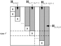
Figure 9: A matrix that satisfies (33), (34) and (35) as in Lemma 7.

Proof.

We use induction as follows.

i) The lemma is true for $N=1$.

ii) Assume that the lemma is true for all $N=1,\ldots,t$. For $N=t+1$:

First, because the upper left $(N-1)\times(N-1)$ submatrix of $\bm{H}$ satisfies the induction assumption, each of $\bm{H}$’s first left $N-1$ columns must contain at least one non-zero entry. From (35), the last column of $\bm{H}$ has at least one non-zero entry. Thus, the case of $n=N$ in Property 1 holds for $\bm{H}$.

Next, $\forall 1\leq n\leq N-1$, for any $n\times N$ submatrix of $\bm{H}$, denote it by $\bm{H}^{\prime}$, and its corresponding row indices in $\bm{H}$ by $r(1)<r(2)<\ldots<r(n)$.

• If the last $n$ rows of $\bm{H}$ are selected to form $\bm{H}^{\prime}$, (i.e. $r(i)=i+N-n,~{}i=1,\ldots,n$), from (34), the columns $N-n,\ldots,N-1$ each has one non-zero entry, namely, $\bm{H}_{N-n+1,N-n},\ldots,\bm{H}_{N,N-1}$.

• Otherwise, there exists a row $r^{*}$, $r^{*}\geq N-n+1$, which is not selected in $\bm{H}^{\prime}$ (cf. Figure 9). In this case, the row indices of $\bm{H}^{\prime}$ can be partitioned into two subsets: $\exists i(\in\{1,2,\ldots,n\}),r(1)<\ldots<r(i)\leq r^{*}-1$ and $r^{*}+1\leq r(i+1)<\ldots\leq r(n)$. On the one hand, note that the upper left $(r^{*}-1)\times(r^{*}-1)$ submatrix of $\bm{H}$ satisfies the induction assumption. Thus, among the first $r^{*}-1$ columns of the rows $r(1),\ldots,r(i)$, there exists $i$ columns each of which has one non-zero entry. On the other hand, from (34), $\bm{H}_{r(i+1),r(i+1)-1},\ldots,\bm{H}_{r(n),r(n)-1}$ are all non-zero, and none of these non-zero entries appears in the first $r^{*}-1$ columns. Therefore, there exist $n$ columns of $\bm{H}^{\prime}$ such that each of them has at least one non-zero entry.

∎

We now prove Lemma 6.

Proof of Lemma 6.

Clearly, Property 1 is implied by the non-zero diagonal property.

To prove that the non-zero diagonal property is also implied by Property 1, we use induction on $\bm{N}$ as follows.

i) For $N=1$, the non-zero diagonal property is implied by Property 1.

ii) Assume that $\forall N\leq t,(t\geq 1,)$ the non-zero diagonal property is implied by Property 1.

For $N=t+1$, we use another induction on the number of rows $n$ of submatrices of $\bm{H}$ in proving a non-zero permuted diagonal property.

a) For $n=1$, directly from Property 1, any $n\times N$ submatrix of $\bm{H}$ (i.e., any row of $\bm{H}$) has at least one non-zero entry.

b) Assume that $\forall n\leq t<N$, $\forall n\times N$ submatrix of $\bm{H}$, denoted by $\bm{H}^{\prime}$, it has the following property:

$$\exists\pi(i)~{}(i=1,\ldots,n)\text{ that satisfies }\pi(i)\neq\pi(j),\forall i\neq j,$$

$$s.t.~{}\bm{H}^{\prime}_{i,\pi(i)}\neq 0.$$ (36)

Figure 10: The matrix $\bm{H}^{\prime}$ in the proof of Lemma 6.

For $n=t+1$, from the induction assumption b), there exists a non-zero permutated diagonal for the $(n-1)\times N$ submatrix $\bm{H}^{\prime}_{[2:n],[1:N]}$: WLOG, assume that it corresponds to $\forall i=2,\ldots,n,\bm{H}^{\prime}_{i,i-1}\neq 0$ (cf. Figure 10.)

Now, we use proof by contradiction, and assume that $\bm{H}^{\prime}$ does not have a non-zero permuted diagonal. Then, the sub-row $\bm{H}^{\prime}_{1,[n,N]}$ must be all zero, because otherwise any non-zero entry within $\bm{H}^{\prime}_{1,[n,N]}$ will form a non-zero permuted diagonal of $\bm{H}^{\prime}$ with $\bm{H}^{\prime}_{i,i-1}(i=2,\ldots,n)$. From Property 1, the $1^{st}$ row of $\bm{H}^{\prime}$ must have at least one non-zero entry. WLOG, assume that $\bm{H}^{\prime}_{1,1}$ is non-zero. Then, the sub-row $\bm{H}^{\prime}_{2,[n,N]}$ must be all-zero, because otherwise any non-zero entry within $\bm{H}^{\prime}_{2,[n,N]}$ will form a non-zero permuted diagonal of $\bm{H}^{\prime}$ with $\bm{H}^{\prime}_{1,1}$ and $\bm{H}^{\prime}_{i,i-1}(i=3,\ldots,n)$. From Property 1, the first two rows of $\bm{H}^{\prime}$ must have at least two columns each of which has at least one non-zero entry. Since $\bm{H}^{\prime}_{2,1}\neq 0$, there is at least one more column of $\bm{H}^{\prime}_{[1,2],[1,N]}$ that has at least one non-zero entry. WLOG, assume that the sub-column $\bm{H}^{\prime}_{[1,2],2}$ has at least one non-zero entry, (cf. the shaded area in Figure 10).

Similarly, consider the $r^{th}$ row of $\bm{H}^{\prime}$. Note that the submatrix $\bm{H}^{\prime}_{[1:r-1],[1:r-1]}$ satisfies (33), (34) and (35), and hence satisfies Property 1 by Lemma 7. From the induction assumption ii), $\bm{H}^{\prime}_{[1:r-1],[1:r-1]}$ has a non-zero permuted diagonal. Then, the sub-row $\bm{H}^{\prime}_{r,[n,N]}$ must be all-zero, because otherwise any non-zero entry within $\bm{H}^{\prime}_{r,[n,N]}$ will form a non-zero permuted diagonal of $\bm{H}^{\prime}$ with the non-zero permuted diagonal of $\bm{H}^{\prime}_{[1:r-1],[1:r-1]}$ and $\bm{H}^{\prime}_{i,i-1}(i=r+1,\ldots,n)$.

Therefore, the submatrix $\bm{H}^{\prime}_{[1,N],[n,N]}$ must be all-zero. This implies that there are only $n-1$ (instead of $n$) columns of $\bm{H}^{\prime}$ each of which has at least one non-zero entry, and hence contradicts with Property 1. ∎

YUE ZHAO (S’06, M’11) is an assistant professor of Electrical and Computer Engineering at Stony Brook University. He received the B.E. degree in Electronic Engineering from Tsinghua University, Beijing, China in 2006, and the M.S. and Ph.D. degrees in Electrical Engineering from the University of California, Los Angeles (UCLA), Los Angeles in 2007 and 2011, respectively. His current research interests include smart grid, renewable energy integration, optimization theory, stochastic control, and statistical signal processing.

Andrea Goldsmith (S’90, M’93, SM’99, F’05) is the Stephen Harris professor in the School of Engineering and a professor of Electrical Engineering at Stanford University. She was previously on the faculty of Electrical Engineering at Caltech. Dr. Goldsmith co-founded and served as CTO for two wireless companies: Wildfire.Exchange, which develops software-defined wireless network technology for cloud-based management of WiFi systems, and Quantenna Communications, Inc., which develops high-performance WiFi chipsets. She has previously held industry positions at Maxim Technologies, Memorylink Corporation, and AT&T Bell Laboratories. She is a Fellow of the IEEE and of Stanford, and has received several awards for her work, including the IEEE ComSoc Edwin H. Armstrong Achievement Award as well as Technical Achievement Awards in Communications Theory and in Wireless Communications, the National Academy of Engineering Gilbreth Lecture Award, the IEEE ComSoc and Information Theory Society Joint Paper Award, the IEEE ComSoc Best Tutorial Paper Award, the Alfred P. Sloan Fellowship, the WICE Outstanding Achievement Award, and the Silicon Valley/San Jose Business Journal’s Women of Influence Award. She is author of the book “Wireless Communications” and co-author of the books “MIMO Wireless Communications” and “Principles of Cognitive Radio,” all published by Cambridge University Press, as well as an inventor on 28 patents. She received the B.S., M.S. and Ph.D. degrees in Electrical Engineering from U.C. Berkeley. Dr. Goldsmith has served as editor for the IEEE Transactions on Information Theory, the Journal on Foundations and Trends in Communications and Information Theory and in Networks, the IEEE Transactions on Communications, and the IEEE Wireless Communications Magazine as well as on the Steering Committee for the IEEE Transactions on Wireless Communications. She participates actively in committees and conference organization for the IEEE Information Theory and Communications Societies and has served on the Board of Governors for both societies. She has also been a Distinguished Lecturer for both societies, served as President of the IEEE Information Theory Society in 2009, founded and chaired the Student Committee of the IEEE Information Theory Society, and chaired the Emerging Technology Committee of the IEEE Communications Society. At Stanford she received the inaugural University Postdoc Mentoring Award, served as Chair of Stanford’s Faculty Senate in 2009, and currently serves on its Faculty Senate, Budget Group, and Task Force on Women and Leadership.

H. Vincent Poor (S’72, M’77, SM’82, F’87) received the Ph.D. degree in electrical engineering and computer science from Princeton University in 1977. From 1977 until 1990, he was on the faculty of the University of Illinois at Urbana-Champaign. Since 1990 he has been on the faculty at Princeton, where he is the Dean of Engineering and Applied Science, and the Michael Henry Strater University Professor of Electrical Engineering. He has also held visiting appointments at several other institutions, most recently at Imperial College and Stanford. His research interests are in the areas of information theory, stochastic analysis and statistical signal processing, and their applications in wireless networks and related fields such as smart grid. Among his publications in these areas is the recent book Mechanisms and Games for Dynamic Spectrum Allocation (Cambridge University Press, 2014). Dr. Poor is a member of the National Academy of Engineering and the National Academy of Sciences, and is a foreign member of the Royal Society. He is also a fellow of the American Academy of Arts and Sciences and of other national and international academies. He received a Guggenheim Fellowship in 2002 and the IEEE Education Medal in 2005. Recent recognition of his work includes the 2014 URSI Booker Gold Medal, the 2015 EURASIP Athanasios Papoulis Award, the 2016 John Fritz Medal, and honorary doctorates from Aalborg University, Aalto University, HKUST, and the University of Edinburgh.

References

- [1] H. Gharavi and R. Ghafurian, “Smart grid: the electric energy system of the future,” Proc. IEEE, vol. 99, no. 6, pp. 917 – 921, June 2011.
- [2] Y. Liu, P. Ning, and M. Reiter, “False data injection attacks against state estimation in electric power grids,” ACM Transactions on Information and System Security, vol. 14, no. 1, Article 13, May 2011.
- [3] A.-H. Mohsenian-Rad and A. Leon-Garcia, “Distributed internet-based load altering attacks against smart power grids,” IEEE Transactions on Smart Grid, vol. 2, no. 4, pp. 667–674, December 2011.
- [4] Y. Liang, H. V. Poor, and S. Shamai, “Information theoretic security,” Found. Trends Commun. Inf. Theory, vol. 5, no. 4, pp. 355–580, April 2009.
- [5] J. Salmeron, K. Wood, and R. Baldick, “Analysis of electric grid security under terrorist threat,” IEEE Transactions on Power Systems, vol. 19, no. 2, pp. 905 – 912, May 2004.
- [6] M. Kezunovic, “Smart fault location for smart grids,” IEEE Transactions on Smart Grid, vol. 2, no. 1, pp. 11–22, March 2011.
- [7] Y. Zhao, A. Goldsmith, and H. V. Poor, “On PMU location selection for line outage detection in wide-area transmission networks,” Proc. of IEEE Power and Energy Society General Meeting, pp. 1–8, July 2012.
- [8] Y. Zhao, R. Sevlian, R. Rajagopal, A. Goldsmith, and H. V. Poor, “Outage detection in power distribution networks with optimally-deployed power flow sensors,” in Proc. of IEEE Power and Energy Society General Meeting, 2013.
- [9] A. Tajer, S. Kar, H. V. Poor, and S. Cui, “Distributed joint cyber attack detection and state recovery in smart grids,” Proc. of IEEE International Conference on Smart Grid Communications (SmartGridComm), pp. 202 –207, October 2011.
- [10] O. Kosut, L. Jia, R. J. Thomas, and L. Tong, “Malicious data attacks on the smart grid,” IEEE Transactions on Smart Grid, vol. 2, pp. 645 – 658, Oct. 2011.
- [11] K. C. Sou, H. Sandberg, and K. H. Johansson, “On the Exact Solution to a Smart Grid Cyber-Security Analysis Problem,” IEEE Transactions on Smart Grid, vol. 4, no. 2, pp. 856 – 865, Jun. 2013.
- [12] J. Hendrickx, K. H. Johansson, R. Jungers, H. Sandberg, and K. C. Sou, “Efficient computations of a security index for false data attacks in power networks,” eprint arXiv:1204.6174.
- [13] A. Teixeira, H. Sandberg, G. Dan, and K. H. Johansson, “Optimal power flow: closing the loop over corrupted data,” Proc. American Control Conference, pp. 3534 – 3540, Jun. 2012.
- [14] L. Jia, J. Kim, R. J. Thomas, and L. Tong, “Impact of Data Quality on Real-Time Locational Marginal Price,” IEEE Transactions on Power Systems, vol. 29, no. 2, pp. 627 – 636, Mar. 2014.
- [15] J. Kim and L. Tong, “On Topology Attack of a Smart Grid: Undetectable Attacks and Countermeasures,” IEEE Journal on Selected Areas in Communications, vol. 31, no. 7, pp. 1294 – 1305, Jul. 2013.
- [16] A. Giani, E. Bitar, M. Garcia, M. McQueen, P. Khargonekar, and K. Poolla, “Smart grid data integrity attacks: characterizations and countermeasures,” Proc. IEEE International Conference on Smart Grid Communications (SmartGridComm), pp. 232–237, October 2011.
- [17] T. T. Kim and H. V. Poor, “Strategic protection against data injection attacks on power grids,” IEEE Transactions on Smart Grid, vol. 2, no. 2, pp. 326–333, June 2011.
- [18] R. B. Bobba, K. M. Rogers, Q. Wang, H. Khurana, K. Nahrstedt, and T. J. Overbye, “Detecting false data injection attacks on dc state estimation,” Proc. Workshop on Secure Control Systems, Apr. 2010.
- [19] J. Weimer, S. Kar, and K. H. Johansson, “Distributed detection and isolation of topology attacks in power networks,” Proc. 1st international conference on High Confidence Networked Systems, pp. 65–72, July 2012.
- [20] F. Pasqualetti, F. Dorfler, and F. Bullo, “Attack detection and identification in cyber-physical systems,” IEEE Transactions on Automatic Control, vol. 58, no. 11, pp. 2715–2729, 2013.
- [21] H. Fawzi, P. Tabuada, and S. Diggavi, “Secure estimation and control for cyber-physical systems under adversarial attacks,” eprint arXiv:1205.5073.
- [22] ——, “Security for control systems under sensor and actuator attacks,” Proc. IEEE 51st Annual Conference on Decision and Control (CDC), pp. 3412–3417, December 2012.
- [23] A. J. Wood and B. F. Wollenberg, Power Generation, Operation, and Control, 2nd ed. John Wiley and Sons, 1996.
- [24] E. J. Candes and T. Tao, “Decoding by linear programming,” IEEE Transactions on Information Theory, vol. 51, no. 12, pp. 4203 – 4215, Dec. 2005.
- [25] K. Reinschke, Multivariable Control - A Graph-Theoretic Approach. New York: Springer-Verlag, Lecture Notes in Control and Information Sciences, vol. 108, 1988.
- [26] R. Johnston, G. Barton, and M. Brisk, “Determination of the generic rank of structural matrices,” Int. J. Control, vol. 40, pp. 257 – 264, 1984.
- [27] M. R. Henzingera, S. Raob, and H. N. Gabow, “Computing vertex connectivity: new bounds from old techniques,” Journal of Algorithms, vol. 34, no. 2, pp. 222 – 250, February 2000.
- [28] V. Vazirani and M. Yannakakis, “Suboptimal cuts: Their enumeration, weight and number,” Automata, Languages and Programming, pp. 366–377, 1992.
- [29] R. D. Zimmerman, C. E. Murillo-Sanchez, and R. J. Thomas, “MATPOWER steady-state operations, planning and analysis tools for power systems research and education,” IEEE Transactions on Power Systems, vol. 26, no. 1, pp. 12 – 19, Feb. 2011.
- [30] T. Baldwin, L. Mili, J. M.B. Boisen, and R. Adapa, “Power system observability with minimal phasor measurement placement,” IEEE Transactions on Power Systems, vol. 8, no. 2, pp. 707 – 715, May 1993.