Analytic Materials

Abstract

The theory of inhomogeneous analytic materials is developed. These are materials where the coefficients entering the equations involve analytic functions. Three types of analytic materials are identified. The first two types involve an integer $p$. If $p$ takes its maximum value then we have a complete analytic material. Otherwise it is incomplete analytic material of rank $p$. For two-dimensional materials further progress can be made in the identification of analytic materials by using the well-known fact that a $90^{\circ}$ rotation applied to a divergence free field in a simply connected domain yields a curl-free field, and this can then be expressed as the gradient of a potential. Other exact results for the fields in inhomogeneous media are reviewed. Also reviewed is the subject of metamaterials, as these materials provide a way of realizing desirable coefficients in the equations.

1 Introduction

Nearly all linear equations of physics (including static equations, heat and diffusion equations, and wave equations) can be written in the form of a system of second order partial differential equations.

$$\nabla\cdot\left[{\bf L}({\bf x})\nabla{\bf u}({\bf x})\right]+{\bf B}({\bf x})\cdot\nabla{\bf u}({\bf x})+{\bf A}({\bf x}){\bf u}({\bf x})={\bf r}({\bf x}),$$ (1.1)

or in component form

$$\frac{\partial}{\partial x_{j}}\left[L_{j\alpha i\beta}({\bf x})\frac{\partial u_{\beta}({\bf x})}{\partial x_{i}}\right]+B_{\alpha i\beta}({\bf x})\frac{\partial u_{\beta}({\bf x})}{\partial x_{i}}+A_{\alpha\beta}({\bf x})u_{\beta}({\bf x})=r_{\alpha}({\bf x}),$$ (1.2)

where $i$ and $j$ are “space indices” taking values from $1$ to $d$, while $\alpha$ and $\beta$ are field indices taking values from $1$ to $m$, and where sums over repeated indices are assumed. It could be the case that $m=1$, in which case the field ${\bf u}({\bf x})=u({\bf x})$ is a scalar field and we can drop the field indices. Here we regard ${\bf L}({\bf x})$, ${\bf B}({\bf x})$, and ${\bf A}({\bf x})$ as the material parameters, ${\bf u}({\bf x})$ and its derivatives as the fields, and ${\bf r}({\bf x})$ as the source term. One can write the equations of electromagnetism, acoustics, elastodynamics, heat conduction, diffusion, and quantum physics in this form. One point to emphasize is that ${\bf x}$ need not represent just spatial variables: we could have $d=4$ where $x_{4}$ represents time and $(x_{1},x_{2},x_{3})$ represents a point in three-dimensional space. Because analytic functions are involved, in the analysis presented here, the coefficients and fields have both real and imaginary parts. However, by taking the real and imaginary parts of (1.2) and expressing them in terms of the real and imaginary parts of ${\bf u}({\bf x})$, it is clear that our analysis also directly applies to certain systems of linear equations with both real coefficients and real potentials. The parameters $x_{i}$ need not represent cartesian coordinates, but instead could represent curvilinear coordinates. Our results apply to partial differential equations of the form (1.2) irrespective of what physical interpretation they may have. In fact the analysis here easily extends to higher order partial differential equations as appropriate, for example, to the treatment of vibrating plates. In multiparticle quantum systems of $n$ particles we may choose $d=3n$ and then ${\bf x}$ represents the coordinates of all $n$ particles.

In our treatment we are considering the equation (1.1) very generally. We do not demand that the material parameters ${\bf L}({\bf x})$, ${\bf B}({\bf x})$, and ${\bf A}({\bf x})$ be real, as they can be complex at constant frequency for the wave equations of electromagnetism, acoustics, elastodynamics if there is loss, or if the frequency is complex, corresponding to growing fields. We do not demand that they have any symmetry properties such as $L_{j\alpha i\beta}({\bf x})=L_{i\beta j\alpha}({\bf x})$ that generally are a consequence of Onsager’s principle and which need not hold if there is some breaking of time-reversal symmetry, such as happens when there is a magnetic field. An example is conductivity in the presence of a magnetic field where the conductivity tensor is not symmetric due to the presence of a magnetic field. Finally we do not demand that say the imaginary part of $L_{i\beta j\alpha}({\bf x})$ be positive semidefinite, in the sense that the quadratic form,

$$f({\bf E})=E_{i\beta}[\mathop{\rm Im}\nolimits(L_{i\beta j\alpha})]E_{j\alpha},$$ (1.3)

is non-negative for all matrices ${\bf E}$ with elements $E_{i\alpha}$, $i=1,2,\ldots,d$, $\alpha=1,2,\ldots,m$, as may happen at constant frequency if there is only loss in the system, as there could be gain.

It is also to be stressed that there is typically a lot of flexibility in writing down the equations that describe a physical system. Of course, a second order equation, like (1.1), always can be written as a system of first order equations by introducing extra variables. For example, by introducing ${\bf F}=\nabla{\bf u}$ (1.1) can be written as

$$\underbrace{\begin{pmatrix}{\bf L}({\bf x})\\ {\bf I}\end{pmatrix}}_{\widetilde{{\bf B}}({\bf x})}\cdot\nabla\underbrace{\begin{pmatrix}{\bf F}({\bf x})\\ {\bf u}({\bf x})\end{pmatrix}}_{\widetilde{{\bf u}}({\bf x})}+\underbrace{\begin{pmatrix}{\bf B}({\bf x})+(\nabla\cdot{\bf L}({\bf x}))&{\bf A}({\bf x})\\ -{\bf I}&0\end{pmatrix}}_{\widetilde{{\bf A}}({\bf x})}\underbrace{\begin{pmatrix}{\bf F}({\bf x})\\ {\bf u}({\bf x})\end{pmatrix}}_{\widetilde{{\bf u}}({\bf x})}=\underbrace{\begin{pmatrix}{\bf r}({\bf x})\\ 0\end{pmatrix}}_{\widetilde{{\bf r}}({\bf x})},$$ (1.4)

that is still of the form (1.1), but without the second order term.

Analytic materials are materials where the material parameters ${\bf L}({\bf x})$, ${\bf B}({\bf x})$, and ${\bf A}({\bf x})$ involve analytic functions, respectively. We will see that they provide a wealth of examples where solutions to the partial differential equations (1.1) can be easily found. These then can serve as benchmarks for numerical calculations, and to gain insight into what manipulations of fields are possible. An early example for the Schrödinger equation was discovered by Berry [10]. He realized that with a potential $V({\bf x})=iV_{0}(e^{iKx_{1}}-1)$ (that is obviously an analytic function of $x_{1}$) one could explicitly work out the strengths of all the diffracted beams. Independently, Milton [95] (see also Sections 14.4 and 14.5 of [94]) considered the scalar wave equation

$$-\nabla\cdot[a_{0}+\delta q({\bf x})]\nabla u({\bf x})=\lambda u({\bf x}),$$ (1.5)

in a periodic medium with $\delta$ being a small constant and with $q({\bf x})$ having Fourier components $\widehat{q}({\bf k})$ vanishing in half of Fourier space, say with $\widehat{q}({\bf k})=0$ if $k_{1}\leq 0$. He showed that the periodic component of the Bloch solution for $u({\bf x})$ shares the property of vanishing in half of Fourier space, and moreover the band structure is exactly the same as for a homogeneous medium, with coefficient $a_{0}$, except possibly for the highest bands. An example was given of a medium with a coefficient

$$q({\bf x})=[\cos(x_{1})+i\sin(x_{1})]r(x_{2},x_{3}),$$ (1.6)

that is clearly an analytic function of $x_{1}$. (Here $r(x_{2},x_{3})$ is an arbitrary bounded function of $x_{1}$ and $x_{2}$.) Perhaps closely related to this (as a dilute array of scatterers can be considered as a periodic medium) is the result of Horsley, Artoni, and La Rocca [54] that an inclusion will not scatter if its moduli only depend on $x_{1}$ and have Fourier components that vanish in half of Fourier space.

In a significant advance, Horsley, King, and Philbin [55] found that a solution of an ordinary differential equation (ODE) as a function of a real valued parameter $z$ could be analytically continued to complex $z$. Then, one could consider a real valued parameter $\gamma$ that is a function of ${\bf x}$, and from an associated trajectory $z(\gamma)$ obtain a solution to the wave equation in the ${\bf x}$ coordinates.

In this paper we show that the range of analytic materials can be vastly expanded. It is to be emphasized that an analytic material need not have any periodicity and may be only defined inside some body $\Omega$ as the analytic continuation of the analytic functions could have singularities outside $\Omega$. This paper concentrates on the general theory. Applications to specific physical equations will be considered elsewhere.

2 A review of some other exact solutions

2.1 Equivalent media using Translations

Suppose we can find tensor fields ${\bf T}({\bf x})$ and ${\bf S}({\bf x})$ such that the equation

$$\nabla\cdot\left[{\bf T}({\bf x})\nabla{\bf u}({\bf x})\right]+{\bf S}({\bf x})\cdot\nabla{\bf u}({\bf x})=0$$ (2.1)

holds for all fields ${\bf u}({\bf x})$. Then, assuming (1.1) has been solved for ${\bf u}({\bf x})$ and subtracting (2.1) from it, we see that ${\bf u}({\bf x})$ solves the equations

$$\nabla\cdot\underline{{\bf L}}({\bf x})\nabla{\bf u}({\bf x})+\underline{{\bf B}}({\bf x})\cdot\nabla{\bf u}({\bf x})+\underline{{\bf A}}({\bf x}){\bf u}({\bf x})={\bf r}({\bf x}),$$ (2.2)

in a translated medium with moduli

$$\underline{{\bf L}}({\bf x})={\bf L}({\bf x})-{\bf T}({\bf x}),\quad\underline{{\bf B}}({\bf x})={\bf B}({\bf x})-{\bf S}({\bf x}),\quad\underline{{\bf A}}({\bf x})={\bf A}({\bf x}).$$ (2.3)

The medium is called a translated medium because (2.3) corresponds to a translation of the moduli in tensor space, at each point ${\bf x}$.

Writing out (2.1) in components we obtain

$$T_{j\alpha i\beta}({\bf x})\frac{\partial^{2}u_{\beta}({\bf x})}{\partial x_{i}\partial x_{j}}+\frac{T_{j\alpha i\beta}({\bf x})}{\partial x_{j}}\frac{\partial u_{\beta}({\bf x})}{\partial x_{i}}+S_{\alpha i\beta}({\bf x})\frac{\partial u_{\beta}({\bf x})}{\partial x_{i}}=0.$$ (2.4)

Clearly, this is satisfied for all fields ${\bf u}({\bf x})$ if and only if

$$T_{j\alpha i\beta}({\bf x})=-T_{i\alpha j\beta}({\bf x}),\quad S_{\alpha i\beta}({\bf x})=-\frac{\partial T_{j\alpha i\beta}({\bf x})}{\partial x_{j}}.$$ (2.5)

Note, in particular, that we could choose ${\bf S}({\bf x})={\bf B}({\bf x})$ and then use (2.5) to determine (non-uniquely) ${\bf T}({\bf x})$. In the setting of (1.1), it is apparent that we can assume ${\bf B}({\bf x})=0$, by, if necessary, translating to an equivalent medium where this holds. This observation is what allowed Norris and Shuvalov [132] (see also [53]) to eliminate such couplings when considering transformation elastodynamics.

It may be the case that the moduli ${\bf L}$, ${\bf B}$, and ${\bf A}$ are independent of ${\bf x}$, and that consequently (1.1) is easily solved for the field ${\bf u}({\bf x})$ when the source term ${\bf r}({\bf x})$ and the boundary conditions are specified. Then, using translations, we obtain solutions for the field ${\bf u}({\bf x})$ in a wide variety of inhomogeneous media.

Translations and equivalent media have played an important role in the theory of composites. See, in particular, Chapters 3, 4, 24, and 25 of [94] and references therein. Notably, Lurie and Cherkaev [85, 86] and Murat and Tartar [115, 155] found that elementary bounds on the effective tensor of the "translated medium" could produce useful, and in many cases sharp, bounds on the effective tensor of the original medium.

In the case where the equations (1.1) are the Euler–Lagrange equations of an associated "energy function", the quadratic form associated with a relevant translation usually corresponds to a null-Lagrangian: a functional whose associated Euler-Lagrange equation vanishes identically. There is a large literature on null-Lagrangians–see, for example, [112, 113, 114, 8, 137].

2.2 Equivalent media using coordinate transformations

There is of course an enormous literature on the exact solution of these equations in various coordinate systems when the coefficients ${\bf L}({\bf x})$, ${\bf B}({\bf x})$, and ${\bf A}({\bf x})$ are constant. The simplest are “plane-wave” solutions where ${\bf u}({\bf x})={\bf u}({\bf k}\cdot{\bf x})$ and the wave vector ${\bf k}$, which is not necessarily real, has to be chosen appropriately. One may also try using separation of variables in different co-ordinate systems. In two dimensions there are many exact solutions that involve analytic functions, notably those of Muskhelishvili [116] and Lekhnitskii [74]. Even in three dimensions one can express any solution to Laplace’s equation in a convex body in terms of analytic functions as shown in Section 6.9 of [94]. Green functions with sources in complex space (i.e. with singularities at points ${\bf x}={\bf x}_{0}$ where the elements of ${\bf x}_{0}$ are complex) give useful representations of fields that can sometimes be more suitable than standard representations using, for example, spherical harmonics [38, 131].

Here we are interested in exact solutions where the coefficients ${\bf L}({\bf x})$, ${\bf B}({\bf x})$, and ${\bf A}({\bf x})$ are not constant, which is of course of great practical interest. Many exact solutions can be obtained by mapping over the ideas presented in chapters 3, 4, 5, 6, 7, 8, 9, 14 and 17 in the book of Milton [94] for periodic materials, to materials that are not periodic. These ideas are due to many people, besides myself, so rather than give a very lengthy list, the reader is referred to the many references in my book.

A vast array of solutions to the equations (1.1) can be obtained by a change of variable ${\bf y}={\bf f}({\bf x})$, mapping a solution, or set of solutions, we know (perhaps in a homogeneous medium) into a solution or set of solutions, with new coefficients ${\bf L}^{\prime}({\bf y})$, ${\bf B}^{\prime}({\bf y})$, and ${\bf A}^{\prime}({\bf y})$, and a new source ${\bf r}^{\prime}({\bf y})$. For electromagnetism the major realization of Dolin [39] was that one could interpret this new equation as solving the equations in a new medium with a new anisotropic permittivity $\mbox{\boldmath${\varepsilon}$}({\bf y})$ and a new anisotropic permeabilty $\mbox{\boldmath${\mu}$}({\bf y})$: transformation optics, or equivalently transformation electromagnetism, was born. (An english translation of his paper is available at http://www.math.utah.edu/~milton/DolinTrans2.pdf) Among other things, Dolin realized that by making this transformation in empty space one could obtain an inclusion that was invisible to all applied fields. Transformation ideas were also used in [37, 29] to map doubly periodic gratings onto flat gratings. Nicorovici, McPhedran, and Milton [124] found that annular regions with a dielectric constant of $-1$ surrounded by a medium of dielectric constant $1$ should be invisible to (almost) all applied quasistatic fields. Alú and Engheta [1] found that coated spheres at certain frequencies could be invisible to incident plane waves. Inclusions were found [84, 159] that are invisible to plane waves in one direction and that in fact can cloak objects inside them, as experimentally confirmed by Landy and Smith [73]. An earlier paper by Kerker [61] had established that confocal coated ellipsoids could be invisible to long wavelength waves: these are called neutral inclusions and there is a large literature concerning them: see, for example, Section 7.11 in [94], and more recent citations of these papers.

Transformation conductivity was discovered by Luc Tartar, who remarked upon it to Kohn and Vogelius [67]. In section 8.5 of my book [94] I showed how transformation conductivity could be used to obtain a vast array of periodic materials for which one could exactly solve the “cell problem”, i.e., obtain periodic solutions for the current and electric field that have nonzero averages over the unit cell, and consequently obtain exact formulae for the effective conductivity tensor. By making the singular transformation

$${\bf y}={\bf f}({\bf x})=\left(\frac{|{\bf x}|}{2}+1\right)\frac{{\bf x}}{|{\bf x}|}\quad{\rm if}\leavevmode\nobreak\ \leavevmode\nobreak\ 2>|{\bf x}|>0,$$ (2.6)

that maps a punctured ball of radius $2$ to a hollow shell of outer radius $2$ and inner radius $1$, Greenleaf, Lassas, and Uhlmann [44, 45] realized one could cloak objects: not make them visible to any external probing current fields (see also [66]). In the transformed geometry conducting objects within the unit ball $|{\bf y}|=1$ feel no probing current field, and therefore are invisible. This marked the discovery of transformation based cloaking. Transformation ideas also extend to geometric optics [76, 75, 77, 79, 78]; to elasticity [101, 18, 132, 53]; to acoustics [36, 31, 40, 128, 43, 32]; to water waves [40]; to matter waves [161, 43, 42]; to plasmonics [58]; to thermal conduction [47, 142] and to flexural waves [41, 35, 154]. In some sense the transformation idea, that began with the transformation optics work of Dolin [39], is a generalization of the idea of using conformal transformations for preserving solutions to the two-dimensional Laplace’s equation that is so well known.

Besides the exact transformations for the moduli, approximate transformations for the moduli have been developed too. Often these work quite well: see, for example, [24, 25, 30]. Additionally, transformations using complex coordinates have proved useful [138, 28].

Curiously, stimulated by a remark of Alexei Efros (private communication, 2005), Nicolae Nicorovici and myself found in 2005 that anomalous resonance creates cloaking where the cloaking device is outside the cloaking region, although it was not until 2006 that our work was published [104]. (I think, though am not certain, that we were the first to use the word “cloaking” as a scientific term in the published literature, outside computer science, for hiding an object). Anomalous localized resonance was discovered by Nicorovici, McPhedran, and myself [124] and as proved in this 1994 paper provides the mechanism for creating “ghost sources”, that on one side of which the field converges to a smooth field having a singularity at the point of the “ghost source” while on the other side of which the field has enormous oscillations. The discovery of ghost sources and anomalous resonance is most clear from Figure 2 in that paper, reproduced here as Figure 1, - see also equation (12) in the 1994 paper and the text below it. See also the rough unpublished draft [93], written prior to May 1996, that emphasizes the observations made in our published paper, and see also [107] where some errors in [124] are corrected. [Additionally, see the introduction in [103]]. An account of the history of the discovery of anomalous resonance, and of “ghost sources”, that are apparent singularities caused by anomalous resonance, can be found in http://www.maths.dur.ac.uk/lms/104/talks/1072milt.pdf. Anomalous resonance provides one of the most striking examples of unusual behavior in linear inhomogeneous systems. It has the curious property that the boundaries of the resonant regions (where the field blows up as the loss tends to zero) move as the source moves. Whereas normal resonances are associated with poles, anomalous resonance seems to be associated with essential singularities [123, 3].

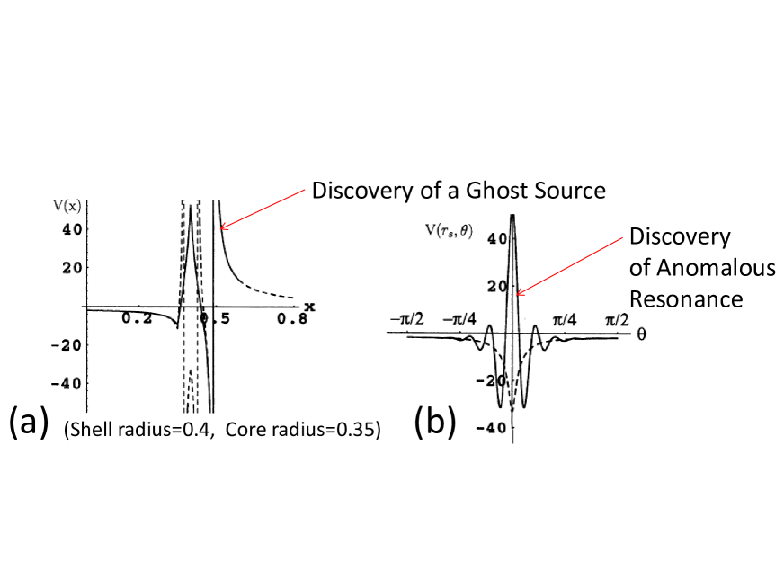
Figure 1: Reproduction, with permission, of Figure 2 of [124] highlighting our discoveries of ghost sources and anomalous resonance. The red arrows and accompaning text are new and are inserted to empasize our findings. Note the apparent divergence in the potential at a radius of $0.52$ in Figure (a) which is outside the shell radius of 0.40. Also in Figure (b) note the large oscillations of the potential showing the anomalous resonance.

Amazingly when the loss is small, or even when there is no loss, anomalous resonance has the incredible feature that although energy produced by a suitably placed constant power source when it is turned on propagates in all directions, at very long times essentially all the energy gets funnelled to the anomalously resonant fields, where it continues to build up with growing fields if there is no loss, or is dissipated into heat if there is a small amount of loss [104]–see in particular figures 4 and 5, and the proof in section 3, also see [105, 160]). The beautiful subsquent numerical simulations made by Nicolae Nicorovici were downloaded so many times that our paper [127]) was in 2007 the most downloaded paper in the journals of the Optical Society of America, with about 13,000 downloads. There is now a substantial body of work that has explored cloaking due to anomalous resonance resonance: see [106, 126, 125, 2], and the references below.

It is to be emphasized that while the original proofs were for a finite but arbitrary number of dipole sources, or polarizable particles in two-dimensional quasistatics, or a single dipole source or polarizable particle in three-dimensional quasistatics, or for a single dipole source or polarizable particle at finite frequency in two dimensions [104]), the cloaking extends to particles that are small compared to the wavelength of the anomalous resonance [11], and to sources of finite size [3, 65, 4, 118, 90, 80]. Sometimes the cloaking is only partial [19] or nonexistent [104, 3, 65, 135]; and it also extends to more general sources and polarizable particles at finite wavelength [126, 63, 135, 120]. Most significantly, Nguyen has recently rigorously proved that for two-dimensional quasistatics, arbitrarily shaped passive objects of small but finite size that are near the annulus are completely cloaked in the limit as the loss in the system tends to zero [119].

Also it is to be emphasized that anomalous resonance and the associated cloaking holds also for magnetoelectric and thermoelectric systems (see section 6 in [107]) and for elasticity [5, 81], which is why I prefer the term cloaking due to anomalous resonance rather than plasmonic cloaking [126, 89]. While in electromagnetism the anomalous resonance is caused by surface plasmons, surface plasmons do not in general have the characteristic feature of anomalous resonant fields that (in theory) they are increasingly confined to a localized region dependent of the position of the sources as the loss in the system goes to zero (or as the time goes to infinity in a loss-less system, with almost time harmonic sources whose amplitude is zero or extremely close to zero in the far distant past). Cloaking due to complementary media, discovered by Lai, Chen, Zhang, and Chan [69], is also caused by anomalous resonance: note the highly oscillating fields near the cloaked inclusions in their numerical simulations. I must admit I was a bit skeptical of this type of cloaking when it first appeared, but Nguyen and Nguyen [122, 121] have now given a rigorous proof of this type of cloaking under certain circumstances.

In 2009 I remembered that the anomalous resonant fields must be caused by polarization charges, and therefore that one should be able to get the same effect by active sources in a homogeneous medium. This gave birth to the subject of active exterior cloaking for conductivity [48, 52], for acoustics in two-dimensions and three-dimensions [48, 49, 51, 53, 129] and for elastodynamics [130]. In a beautiful twist of the idea, O’Neill, Selsil, McPhedran, Movchan, Movchan, and Moggach [133, 134] found that for the plate equation one could get excellent exterior cloaking without enormous fields if one relaxed the requirement that the cloak create a quiet zone and instead require only that it cloak a given object. The main reason that enormous fields are not needed is that the plate equation has the desirable property that the Green’s function is bounded.

3 Metamaterials

Metamaterials are basically composite materials, with properties not normally found in nature. They allow a wide range of parameters ${\bf L}({\bf x})$, ${\bf B}({\bf x})$, and ${\bf A}({\bf x})$ to be realized, thus enabling one to approximately realize many exact solutions. An excellent, though not completely comprehensive, survey of electromagnetic metamaterials can be found in the slides of Sergei Tretyakov (https://users.aalto.fi/~sergei/Tretyakov_slides_Metamaterials2015.pdf). As he mentions, they have been studied since at least 1898. In particular, Brown [17] realized that media with short wires could give rise to effective refractive indices less than one. Maz’ya and Hänler [87] realized that one could obtain asymptotic solutions when part of the domain is cut into tubes that transport the current. Schelkunoff and Friis [141] and Lagarkov et.al. [68] realized one could get artificial magnetism with arrays of split rings (see also [157]). Experiments showing negative magnetic permeabilty were performed by Lagarkov et.al. [68]. Materials with simultaneous negative permittivity and permeability, and hence a negative refractive index, that were studied by Veselago [156], were experimentally realized by Shelby, Smith, and Schultz [146]. These materials have the curious property that the wave crests move opposite to the group velocity, i.e., opposite to the direction of energy flow. Waves with such properties were studied as early as 1904 in the works of Lamb [72] and Schuster [144].

In fact, in theory, at constant frequency, one can get any desired pair $(\mbox{\boldmath${\varepsilon}$},\mbox{\boldmath${\mu}$})$, of permittivity tensor ${\varepsilon}$ and permeability tensor ${\mu}$ provided they are both almost real [97]. Of particular interest are materials where at a given frequency the dielectric constant is close to zero: these epsilon near zero (ENZ) materials have remarkable properties [152] and can be used to design new types of theoretical "electromagnetic circuits" [108, 109] that operate at a single frequency. By laminating a material having a negative dielectric constant over a range of frequencies, with a material having a positive dielectric constant one can get hyperbolic materials where, over a range of frequencies, the dielectric tensor has both positive and negative eigenvalues, and these can be used as hyperlenses [56, 140, 139, 83]. In the infrared and optical regime the building blocks for constructing metamaterials have been plasmonic materials like silver, gold, and silicon carbide that have a negative real part to the permittivity, and a comparatively small imaginary part, though at best it is still about one tenth of the magnitude of the real part. Now, new better performing plasmonic materials are available [117].

Interestingly, in three dimensions, but not in two-dimensions, one can combine materials with positive Hall-coefficient to obtain a composite with negative Hall-coefficient [15, 59]: see also [16], thereby destroying the argument that in classical physics it is the sign of the Hall coefficient which tells one the sign of the charge carrier. A fantastic experimental confirmation of this result has been obtained in [62].

My own interest in metamaterials was sparked by some brilliant experiments of Roderic Lakes [70], that showed it was possible to get isotropic foams with a negative Poisson’s ratio that widen as they stretched. Subsequently I obtained the first rigorous proof [92] that negative Poisson ratio (Auxetic) materials exist within the framework of continuum elasticity, without voids or sliding surfaces. Although I did not draw attention to it at the time, one model that I came up with, having hexagonal spoked wheels linked by deformable parallelogram structures, had the interesting property that when the spoken wheels and linkages were almost rigid then its only easy mode of deformation is a dilation over some (not infinitesimal) window of strains. Another astoundingly simple two-dimensional dilational material consisting of rotating squares, was discovered by Grima and Evans [46]. It was related to some models that Sigmund [149] had found earlier, both in two and three dimensions, but which had sliding surfaces. In fact, the rotating square model was known to Pauling [136], although he does not appear to have made a connection with Auxeticity.

Three dimensional dilational materials without sliding surfaces have been discovered more recently [98, 99], and approximations of such structures have been built and tested [21]. Amazingly, any fourth-order tensor that is positive definite and has the symmetries of elasticity tensors, can be realized as the effective elasticity tensor of a mixture of a sufficiently compliant phase and a sufficiently stiff phase [102]. The building blocks for the construction are pentamode materials: elastic materials that essentially can only support one stress, but that stress can be any given matrix. In an incredible feat of three-dimensional lithography, these have actually been built [57] and used to construct an “unfeelability cloak” [23]. More generally it is theoretically possible to design materials whose macroscopically affine deformations are constrained to lie on any desired trajectory in the 6-dimensional deformation space, excluding deformations where the structure collapses to a lower dimension [98]). Also a lot of progress has been made on the characterization of the possible effective elasticity tensors of three-dimensional printed materials when the elastic moduli, and volume fraction, of the constituent material are known, assuming there is just one constituent material plus void [100].

It is also possible to combine three materials (or two plus void) all of which by themselves expand when heated to obtain a composite which contracts when heated, or alternatively which expands more than the constituent materials [71, 150, 151].

One can combine materials with positive mass density to obtain composites with negative effective mass density [147, 82]; and one can obtain materials with, at a given frequency, anisotropic and even complex effective mass density [143, 101, 20]. In fact, it follows directly from the work of Movchan and Guenneau [111] that there is a close link between negative effective mass density in antiplane elasticity and negative magnetic permeability: in cylindrical geometries the Helmholtz equation is common to both physical phenomena. Moreover, as pointed out by Milton and Willis [110], in metamaterials Newton’s law $F=ma$ should be replaced by a law where the force depends on the acceleration at at previous times, and not just at the present time since it takes some time for the constituents to move: they do not necessarily move together in lock step motion.

However, with respect to the results in the previous paragraph, attention should be drawn to the pioneering work of Auriault and Bonnet [7, 6] who studied homogenization in high contrast elastic media and found that the effective density could be anisotropic and frequency dependent. To quote them "The monochromatic macroscopic behavior is elastic, but with an effective density $\varrho^{\rm eff}$ of tensorial character and depending on the pulsation". Moreover they realized that the effective density could be negative. Referring to a figure they say "hatched areas correspond to negative densities $\varrho^{\rm eff}$, i.e., to stopping bands." A more rigorous approach to the same problem was developed by Zhikov [162]. Smyshlyaev [153] extended the analysis to elastic waves propagating in extremely anisotropic media. The extension to Maxwell’s equations was done by Bouchitte and Schweizer [12] and Cherednichenko and Cooper [33].

Noteworthy is that in 1982, McPhedran, Botten, Craig, Nevière and Maystre [88] had realized that conventional homogenization was not appropriate for high contrast lossy lamellar gratings, even in the long wavelength limit. Also, in 1985, in his ensemble average framework for studying waves in composites, Willis [158] proved that his “effective density” operator is a second order tensor.

What is especially remarkable is that Camar-Eddine and Seppecher [26, 27]) have been able to completely characterize, in a certain sense, all possible homogenized behaviors, including non-local ones, in mixtures of high contrast conducting materials and high contrast linear elastic materials. The key elements are dumbbell shaped inclusions, on many scales. The highly conducting dumbbells, or almost rigid dumbbells, provide a non-local interaction between the balls at the ends when the radius of the bar joining the balls shrinks to zero. The material near the bar is affected by the potential or displacement of the bar, but this scales away as the radius of the bar shrinks to zero. So one can treat it as if the bar is absent, but with a non-local interaction between the balls.

At the discrete level, all possible dynamic behaviors of linear mass-spring networks have been completely characterized [50]. This gives hope that a simllar characterization may be possible in the continuum case. Whether such a characterization will have any practical significance is not at all clear. In the case of the paper of Camar-Eddine and Seppecher [27] at any finite deformation non-linear effects are important in the delicate structures that are needed to achieve some of the exotic linear behaviors.

Specific examples of exotic behaviors in high contrast elastic systems have been given by Seppecher, Alibert, and dell’Isola [145]. Other exotic behaviors of high contrast composites have been found and explored [64, 13, 14, 9, 34, 148, 96, 60]. The architect/artist Boris Stuchebryukov has constructed incredible metamaterials made from parallelogram mechanisms using razor blades (see the beautiful videos https://www.youtube.com/watch?v=l8wrT2YB5s8 and https://www.youtube.com/watch?v=AkUn8nFd8mk).

We mention too, that part of the reason for the surge of interest in these metamaterials arises because precision three-dimensional lithography and printing techniques [57, 22, 21, 91] now allow one to tailor beautiful structures with desired properties. Still there are limitations: usually one wants the cell size to be small and this restricts the size of the overall sample, since in three dimensions the number of cells scales as the cube of the sample side. For this reason metasurfaces and planar lattice materials may hold more promise for practical applications.

4 Analytic Materials of Type One

Suppose ${\bf x}\in\mathbb{R}^{d}$ and one has a basis of $d$-complex wavevectors ${\bf k}^{(\ell)}$, $\ell=1,2,\ldots,d$. Suppose further that

$$L_{j\alpha i\beta}({\bf x})k^{(\ell)}_{i}=P^{(\ell)}_{\alpha j\beta}({\bf x}\cdot{\bf k}^{(\ell)}),\quad B_{\alpha i\beta}({\bf x})k^{(\ell)}_{i}=Q^{(\ell)}_{\alpha\beta}({\bf x}\cdot{\bf k}^{(\ell)}),\quad A_{\alpha\beta}({\bf x})=A_{\alpha\beta},\quad r_{\alpha}({\bf x})=\sum_{\ell}S_{\alpha\ell}({\bf x}\cdot{\bf k}^{(\ell)}),$$ (4.1)

where the coefficients $A_{\alpha\beta}$ are independent of ${\bf x}$, and $P^{(\ell)}_{i\alpha\beta}(z)$, $Q^{(\ell)}_{\alpha\beta}(z)$ and $S_{\beta\ell}(z)$ are analytic functions of $z$. Note that since the ${\bf k}^{(\ell)}$ are a basis, (4.1) completely determines all elements of ${\bf L}({\bf x})$ and ${\bf B}({\bf x})$.

We look for a solution ${\bf u}({\bf x})$ with elements $u_{\beta}$ of the form

$$u_{\beta}({\bf x})=\sum_{\ell}f_{\beta\ell}({\bf x}\cdot{\bf k}^{(\ell)}),$$ (4.2)

where the $f_{\beta\ell}(z)$ are analytic functions of $z$. Then we have

$$\frac{\partial u_{\beta}({\bf x})}{\partial x_{i}}=\sum_{\ell}k_{i}^{(\ell)}f^{\prime}_{\beta\ell}({\bf x}\cdot{\bf k}^{(\ell)}),$$ (4.3)

and consequently

$$L_{j\alpha i\beta}({\bf x})\frac{\partial u_{\beta}({\bf x})}{\partial x_{i}}=\sum_{\ell}L_{j\alpha i\beta}({\bf x})k_{i}^{(\ell)}f^{\prime}_{\beta\ell}({\bf x}\cdot{\bf k}^{(\ell)})=\sum_{\ell}P^{(\ell)}_{\alpha j\beta}({\bf x}\cdot{\bf k}^{(\ell)})f^{\prime}_{\beta\ell}({\bf x}\cdot{\bf k}^{(\ell)}),$$ (4.4)

which implies

$$\frac{\partial}{\partial x_{j}}\left[L_{j\alpha i\beta}({\bf x})\frac{\partial u_{\beta}({\bf x})}{\partial x_{i}}\right]=\sum_{\ell}k_{j}^{(\ell)}\left[P^{(\ell)}_{\alpha j\beta}(z)f^{\prime}_{\beta\ell}(z)\right]^{\prime}\biggr{\rvert}_{z={\bf x}\cdot{\bf k}^{(\ell)}}.$$ (4.5)

We also have

$$B_{\alpha i\beta}({\bf x})\frac{\partial u_{\beta}({\bf x})}{\partial x_{i}}=\sum_{\ell}Q^{(\ell)}_{\alpha\beta}({\bf x}\cdot{\bf k}^{(\ell)})f^{\prime}_{\beta\ell}({\bf x}\cdot{\bf k}^{(\ell)}).$$ (4.6)

By substituting these expressions back in our main equation (1.2) we arrive at

$$\sum_{\ell}k_{j}^{(\ell)}\left[P^{(\ell)}_{\alpha j\beta}(z)f^{\prime}_{\beta\ell}(z)\right]^{\prime}+Q^{(\ell)}_{\alpha\beta}(z)f^{\prime}_{\beta\ell}(z)+A_{\alpha\beta}f_{\beta\ell}(z)-S_{\alpha\ell}(z)\biggr{\rvert}_{z={\bf x}\cdot{\bf k}^{(\ell)}}=0.$$ (4.7)

So the $f_{\beta\ell}(z)$ should satisfy

$$k_{j}^{(\ell)}\left[P^{(\ell)}_{\alpha j\beta}(z)\right]^{\prime}f^{\prime}_{\beta\ell}(z)+k_{j}^{(\ell)}P^{(\ell)}_{\alpha j\beta}(z)f^{\prime\prime}_{\beta\ell}(z)+Q^{(\ell)}_{\alpha\beta}f^{\prime}_{\beta\ell}(z)+A_{\alpha\beta}f_{\beta\ell}(z)-S_{\alpha\ell}(z)=0,$$ (4.8)

for $\alpha=1,2,\ldots,m$, where sums over the repeated indices $j$ and $\beta$ are implied. For fixed $\ell$ this provides $m$ ordinary differential equations for the $m$ unknowns $f_{\beta\ell}(z)$, $\beta=1,2,\ldots,m$. We can rewrite (4.8) in matrix form as

$$\left[{\bf k}^{(\ell)}\cdot{\bf P}^{(\ell)}(z)\right]^{\prime}\left[{\bf f}^{(\ell)}(z)\right]^{\prime}+{\bf k}^{(\ell)}\cdot{\bf P}^{(\ell)}(z)\left[{\bf f}^{(\ell)}(z)\right]^{\prime\prime}+{\bf Q}^{(\ell)}(z)\left[{\bf f}^{(\ell)}(z)\right]^{\prime}+{\bf A}{\bf f}^{(\ell)}(z)={\bf s}^{(\ell)}(z),$$ (4.9)

where for a given $\ell$, ${\bf f}^{(\ell)}(z)$ and ${\bf s}^{(\ell)}(z)$ are at each point $z$, $m$-component vectors with elements $f_{\beta\ell}(z)$ and $S_{\beta\ell}(z)$, $\beta=1,2,\ldots,m$; ${\bf Q}^{(\ell)}(z)$ and ${\bf A}$ are $m\times m$ matrices with elements $Q^{(\ell)}_{\alpha\beta}(z)$ and $A_{\alpha\beta}$; ${\bf P}^{(\ell)}(z)$ is a 3-index object with one space index and two field indices– the $d$-dimensional vector ${\bf k}^{(\ell)}$ acts on the space index of ${\bf P}^{(\ell)}(z)$ leaving a $m\times m$ matrix ${\bf k}^{(\ell)}\cdot{\bf P}^{(\ell)}(z)$ with elements $k_{j}^{(\ell)}P^{(\ell)}_{\alpha j\beta}(z)$.

Note that it could be the case that (4.1), or equivalently (4.9) only holds for $\ell=1,2,\ldots,p$ where $p<d$. In that case we call the material an “incomplete analytic material of type 1, and rank $p$. In the case where $p=d$ we have a “complete analytic material of type 1”, or just simply, an “analytic material of type 1”.

Analytic materials are easily generated from (4.9). The simplest way to do this is just to arbitrarily pick $d^{2}m^{2}$ analytic functions $P^{(\ell)}_{\alpha j\beta}(z)$, $dm^{2}$ analytic functions $Q^{(\ell)}_{\alpha\beta}(z)$, $m^{2}$ constants $A_{\alpha\beta}$ and $md$ analytic functions $f_{\beta\ell}(z)$, taking care to ensure that the resultant singularities in spatial coordinates lie inside the body $\Omega$. Then choosing the $d^{2}$ constants $k_{j}^{(\ell)}$ so that the vectors ${\bf k}^{(\ell)}$, $\ell=1,2,\ldots,d$ form a basis, we can ensure that (4.9) is satisfied by choosing the left hand side to be our source ${\bf s}^{(\ell)}(z)$ that is then analytic in $z$. Moreover if the given analytic functions are polynomials, then the matrix elements $S_{\alpha\ell}(z)$ will also be polynomials. Such a material would then be a polynomial material – defined as one for which the coefficients and sources are entirely expressed in terms of polynomials, and are such that there is at least one solution for ${\bf u}({\bf x})$ involving polynomials $f_{\beta\ell}(z)$.

Even when there are no sources, i.e., when ${\bf s}^{(\ell)}(z)=0$ for all $\ell$, we could, for example, ensure that (4.9) is satisfied by picking a set of $dm$ analytic functions $e_{\gamma\ell}(z)$, $\ell=1,\ldots,d$, $\gamma=1,\ldots,m$ and choosing the matrix elements $Q^{(\ell)}_{\alpha\beta}(z)$ to be given by

$$Q^{(\ell)}_{\alpha\beta}=-\frac{e_{\beta\ell}(z)}{e_{\gamma\ell}(z)f^{\prime}_{\gamma\ell}(z)}\left\{k_{j}^{(\ell)}[P^{(\ell)}_{\alpha j\eta}(z)]^{\prime}f^{\prime}_{\eta\ell}(z)+k_{j}^{(\ell)}P^{(\ell)}_{\alpha j\eta}(z)f^{\prime\prime}_{\eta\ell}(z)+A_{\alpha\eta}f_{\eta\ell}(z)\right\},$$ (4.10)

where summation over the repeated indices $\gamma$, $j$, and $\eta$ is implied, but no sum is taken over $\ell$.

Undoubtedly, there are many more ways of generating analytic materials. The preceding examples just serve to demonstrate that there exist a wide class of analytic materials.

5 Analytic Materials of Type Two

Suppose one has a basis ${\bf e}^{\ell}$, $\ell=1,2,\ldots,md$ of $d\times m$ matrices such that each ${\bf e}^{\ell}$ is a rank one matrix:

$$e^{\ell}_{i\beta}=k^{(\ell)}_{i}v^{(\ell)}_{\beta},$$ (5.1)

where the $k^{(\ell)}_{i}$ and $v^{(\ell)}_{\beta}$ are complex and do not depend on ${\bf x}$. Assume further that

$$L_{j\alpha i\beta}({\bf x})e^{(\ell)}_{i\beta} = P^{(\ell)}_{j\alpha}({\bf x}\cdot{\bf k}^{(\ell)}),\quad B_{\alpha i\beta}({\bf x})e^{(\ell)}_{i\beta}=Q^{(\ell)}_{\alpha}({\bf x}\cdot{\bf k}^{(\ell)}),$$

$$A_{\alpha\beta}({\bf x})v^{(\ell)}_{\beta} = H_{\alpha}^{(\ell)}({\bf x}\cdot{\bf k}^{(\ell)}),\quad r_{\alpha}({\bf x})=\sum_{\ell}S_{\alpha}^{(\ell)}({\bf x}\cdot{\bf k}^{(\ell)}),$$ (5.2)

where the $P^{(\ell)}_{j\alpha}(z)$, $Q^{(\ell)}_{\alpha}(z)$, $H_{\alpha}^{(\ell)}(z)$ and $S_{\alpha\ell}(z)$ are analytic functions of $z$ but should not be confused with the functions in the previous section.

Now we look for a solution

$$u_{\beta}=\sum_{\ell}v^{(\ell)}_{\beta}f_{\ell}({\bf x}\cdot{\bf k}^{(\ell)}).$$ (5.3)

We get

$$\sum_{\ell}k_{j}^{(\ell)}\left[P^{(\ell)}_{j\alpha}(z)f_{\ell}^{\prime}(z)\right]^{\prime}+Q^{(\ell)}_{\alpha}(z)f_{\ell}^{\prime}(z)+H^{(\ell)}_{\alpha}(z)f_{\ell}(z)-S_{\alpha}^{(\ell)}(z)\biggr{\rvert}_{z={\bf x}\cdot{\bf k}^{(\ell)}}=0.$$ (5.4)

So each function $f_{\ell}(z)$ should solve the $m$ second-order differential equations,

$$k_{j}^{(\ell)}\left[P^{(\ell)}_{\alpha j}(z)\right]^{\prime}f^{\prime}_{\ell}(z)+k_{j}^{(\ell)}P^{(\ell)}_{\alpha j}(z)f^{\prime\prime}_{\ell}(z)+Q^{(\ell)}_{\alpha}(z)f^{\prime}_{\ell}(z)+H^{(\ell)}_{\alpha}(z)f_{\ell}(z)=S_{\alpha}^{(\ell)}(z),$$ (5.5)

for $\alpha=1,2,\ldots,m$. This is generally an overdetermined system of equations, as we have $m$ equations to be satisfied by a single function $f_{\ell}(z)$. So let us make the additional assumption that there exist real or complex constants $c_{\alpha}$ and analytic functions $p^{(\ell)}_{j}(z)$, $q^{(\ell)}(z)$, $h^{(\ell)}(z)$, and $s^{(\ell)}(z)$ such that

$$P^{(\ell)}_{\alpha j}(z)=c_{\alpha}p^{(\ell)}_{j}(z),\quad Q^{(\ell)}_{\alpha}(z)=c_{\alpha}q^{(\ell)}(z),\quad H^{(\ell)}_{\alpha}=c_{\alpha}h^{(\ell)}(z),\quad S_{\alpha}^{(\ell)}(z)=c_{\alpha}s^{(\ell)}(z).$$ (5.6)

Then the fundamental equations (5.5) reduce to

$$k_{j}^{(\ell)}\left[p^{(\ell)}_{j}(z)\right]^{\prime}f^{\prime}_{\ell}(z)+k_{j}^{(\ell)}p^{(\ell)}_{j}(z)f^{\prime\prime}_{\ell}(z)+q^{(\ell)}(z)f^{\prime}_{\ell}(z)+h^{(\ell)}(z)f_{\ell}(z)=s^{(\ell)}(z).$$ (5.7)

Again it could be the case that (5.2) and (5.6) only holds for $\ell=1,2,\ldots,p$ where $p<md$. In that case we call the material an “incomplete analytic material of type 2, and rank $p$. In the case where $p=md$ we have a “complete analytic material of type 2”, or just simply, an “analytic material of type 2”.

As for analytic materials of type one, solutions to (5.7) are easily generated. For example, one could just simply arbitrarily choose all the analytic functions aside from those functions $s^{(\ell)}(z)$ determining the sources (making sure the resultant singularities in spatial coordinates lie the body $\Omega$) and then let the left hand side of (5.7) determine these sources. In the absence of sources one could arbitrarily choose the analytic functions $p^{(\ell)}_{j}(z)$, $q^{(\ell)}(z)$, and $f_{\ell}(z)$ and then to satisfy (5.7) choose

$$h^{(\ell)}(z)=-\left\{k_{j}^{(\ell)}[p^{(\ell)}_{j}(z)]^{\prime}f^{\prime}_{\ell}(z)+k_{j}^{(\ell)}p^{(\ell)}_{j}(z)f^{\prime\prime}_{\ell}(z)+q^{(\ell)}(z)f^{\prime}_{\ell}(z)\right\}/f_{\ell}(z),$$ (5.8)

where the sum over $j$ is implied, but not over $\ell$. Alternatively, if $h^{(\ell)}(z)$ is given, but not $q^{(\ell)}(z)$, then we can divide (5.7) by $f^{\prime}_{\ell}(z)$ to obtain a formula for $q^{(\ell)}(z)$ in terms of the other analytic functions.

6 Analytic Materials of Type Three

Let us again begin with the equations

$$\frac{\partial}{\partial x_{j}}\left[L_{j\alpha i\beta}({\bf x})\frac{\partial u_{\beta}({\bf x})}{\partial x_{i}}\right]+B_{\alpha i\beta}({\bf x})\frac{\partial u_{\beta}({\bf x})}{\partial x_{i}}+A_{\alpha\beta}({\bf x})u_{\beta}({\bf x})=r_{\beta}({\bf x}),$$ (6.1)

and look for solutions of the form

$$u_{\beta}({\bf x})=f_{\beta}(t({\bf x})),$$ (6.2)

where $f_{\beta}(z)$ is an analytic function of $z$, and $t({\bf z})$ is some twice differentiable function mapping $\Omega$ onto a region $\Upsilon$ of the complex plane. We have

$$\frac{\partial u_{\beta}({\bf x})}{\partial x_{i}} = \frac{\partial t({\bf x})}{\partial x_{i}}f^{\prime}_{\beta}(t({\bf x})),$$

$$\frac{\partial^{2}u_{\beta}({\bf x})}{\partial x_{i}\partial x_{j}} = \frac{\partial t({\bf x})}{\partial x_{i}}\frac{\partial t({\bf x})}{\partial x_{j}}f^{\prime\prime}_{\beta}(t({\bf x})+\frac{\partial^{2}t({\bf x})}{\partial x_{i}\partial x_{j}}f^{\prime}_{\beta}(t({\bf x})).$$ (6.3)

Then by simple differentiation,

$$\frac{\partial}{\partial x_{j}}\left[L_{j\alpha i\beta}({\bf x})\frac{\partial u_{\beta}({\bf x})}{\partial x_{i}}\right]=\left[\frac{\partial}{\partial x_{j}}L_{j\alpha i\beta}({\bf x})\right]\frac{\partial u_{\beta}({\bf x})}{\partial x_{i}}+L_{j\alpha i\beta}({\bf x})\frac{\partial^{2}u_{\beta}({\bf x})}{\partial x_{i}\partial x_{j}}$$ (6.4)

$$=\left[\frac{\partial}{\partial x_{j}}L_{j\alpha i\beta}({\bf x})\right]\frac{\partial t({\bf x})}{\partial x_{i}}f^{\prime}_{\beta}(t({\bf x}))+L_{j\alpha i\beta}({\bf x})\frac{\partial t({\bf x})}{\partial x_{i}}\frac{\partial t({\bf x})}{\partial x_{j}}f^{\prime\prime}_{\beta}(t({\bf x})+L_{j\alpha i\beta}({\bf x})\frac{\partial^{2}t({\bf x})}{\partial x_{i}\partial x_{j}}f^{\prime}_{\beta}(t({\bf x})),$$

and

$$B_{\alpha i\beta}({\bf x})\frac{\partial u_{\beta}({\bf x})}{\partial x_{i}}=B_{\alpha i\beta}({\bf x})\frac{\partial t({\bf x})}{\partial x_{i}}f^{\prime}_{\beta}(t({\bf x})),$$ (6.5)

Introducing a set of $m$ functions $h_{\alpha}({\bf x})$ that multiply the equations, the equations that interest us now take the form,

$$\left[h_{\alpha}({\bf x})L_{j\alpha i\beta}({\bf x})\frac{\partial t({\bf x})}{\partial x_{i}}\frac{\partial t({\bf x})}{\partial x_{j}}\right]f^{\prime\prime}_{\beta}(t({\bf x}))$$ (6.6)

$$+\left[h_{\alpha}({\bf x})\frac{\partial}{\partial x_{j}}L_{j\alpha i\beta}({\bf x})\frac{\partial t({\bf x})}{\partial x_{i}}+h_{\alpha}({\bf x})L_{j\alpha i\beta}({\bf x})\frac{\partial^{2}t({\bf x})}{\partial x_{i}\partial x_{j}}+h_{\alpha}({\bf x})B_{\alpha i\beta}({\bf x})\frac{\partial t({\bf x})}{\partial x_{i}}\right]f^{\prime}_{\beta}(t({\bf x}))$$

$$+h_{\alpha}({\bf x})A_{\alpha\beta}({\bf x})f_{\beta}(t({\bf x}))=h_{\alpha}({\bf x})r_{\alpha}({\bf x}),$$

for $\alpha=1,2,\ldots,m$, where there is no sum over $\alpha$, even though it is a repeated index. Now suppose the coefficients in the equations are such that for some analytic functions $G^{L}_{\alpha\beta}(z)$, $G^{L}_{\alpha\beta}(z)$, $G^{B}_{\alpha\beta}(z)$, $G^{A}_{\alpha\beta}(z)$, $g^{r}_{\alpha}(z)$ we have

$$\left[h_{\alpha}({\bf x})L_{j\alpha i\beta}({\bf x})\frac{\partial t({\bf x})}{\partial x_{i}}\frac{\partial t({\bf x})}{\partial x_{j}}\right] = G^{L}_{\alpha\beta}(t({\bf x})),$$

$$\left[h_{\alpha}({\bf x})\frac{\partial}{\partial x_{j}}L_{j\alpha i\beta}({\bf x})\frac{\partial t({\bf x})}{\partial x_{i}}+h_{\alpha}({\bf x})L_{j\alpha i\beta}({\bf x})\frac{\partial^{2}t({\bf x})}{\partial x_{i}\partial x_{j}}+h_{\alpha}({\bf x})B_{\alpha i\beta}({\bf x})\frac{\partial t({\bf x})}{\partial x_{i}}\right] = G^{B}_{\alpha\beta}(t({\bf x})),$$

$$h_{\alpha}({\bf x})A_{\alpha\beta}({\bf x}) = G^{A}_{\alpha\beta}(t({\bf x})),$$

$$h_{\alpha}({\bf x})r_{\alpha}({\bf x}) = g^{r}_{\alpha}(t_{\alpha}({\bf x})),$$ (6.7)

where again there is no sum over the repeated index $\alpha$. Then the equations (6.6) reduce to

$$G^{L}_{\alpha\beta}(z)f^{\prime\prime}_{\beta}(z)+G^{B}_{\alpha\beta}(z)f^{\prime}_{\beta}(z)+G^{A}_{\alpha\beta}(z)f_{\beta}(z)=g^{r}_{\alpha}(z),$$ (6.8)

with $z=t({\bf x})$. We can rewrite (6.8) in the more compact form

$${\bf G}^{L}(z){\bf f}^{\prime\prime}(z)+{\bf G}^{B}(z){\bf f}^{\prime}(z)+{\bf G}^{A}(z){\bf f}(z)={\bf g}^{r}(z),$$ (6.9)

where ${\bf G}^{L}(z)$, ${\bf G}^{B}(z)$, and ${\bf G}^{A}(z)$ are $m\times m$ matrix-valued analytic functions of $z$, by which we mean that their elements $G^{L}_{\alpha\beta}(z)$, $G^{B}_{\alpha\beta}(z)$, and $G^{A}_{\alpha\beta}(z)$ are analytic functions of $z$, and ${\bf g}^{r}({\bf z})$ and ${\bf f}(z)$ are $m$-dimensional vector valued analytic functions of $z$, by which we mean that their elements $g^{r}_{\alpha}({\bf z})$ and $f_{\alpha}(z)$ are analytic functions of $z$. If we have solutions to the system of ordinary differential equations (6.8), say for real values of $z$, and if these solutions can be extended to the region $\Upsilon$ of the complex-plane without any singularities in $\Upsilon$, then automatically by substituting ${\bf z}=t({\bf x})$ we have a solututions to the original inhomogeneous partial differential equation.

Once again, analytic functions that satisfy (6.8) are easily generated: sources could be chosen with $g^{r}_{\alpha}(z)$ determined by the left hand side of (6.8). Or, if the sources are zero, one could pick $m$ analytic functions $e_{\beta}(z)$, $\beta=1,2,\ldots,m$, and set

$$G^{A}_{\alpha\beta}(z)=-\frac{e_{\beta}(z)}{e_{\gamma}(z)f_{\gamma}(z)}\left[G^{L}_{\alpha\eta}(z)f^{\prime\prime}_{\eta}(z)+G^{B}_{\alpha\eta}(z)f^{\prime}_{\eta}(z)\right],$$ (6.10)

in which sums over $\gamma$ and $\eta$ are implied, and the $f_{\alpha}(z)$, $G^{L}_{\alpha\eta}(z)$, and $G^{B}_{\alpha\eta}(z)$ are given analytic functions. Having determined these analytic functions there is a lot of flexibility in choosing coefficients $L_{j\alpha i\beta}({\bf x})$, $B_{\alpha i\beta}$ and $A_{\alpha\beta}({\bf x})$ so that (6.7) is satisfied.

7 Analytic Materials in Two-Dimensions

Two-dimensions is rather special in that if for some vector field ${\bf j}({\bf x})$, $\nabla\cdot{\bf j}({\bf x})=0$ in a region $\Omega$, then we have $\nabla\times{\bf e}=0$, where

$${\bf e}={\bf R}^{\perp}{\bf j},\quad{\rm and}\quad{\bf R}^{\perp}=\begin{pmatrix}0&1\\ -1&0\end{pmatrix}$$ (7.1)

is the matrix for a $90^{\circ}$ pointwise rotation of the vector fields, and in two-dimensions $\nabla\times{\bf e}$ is defined to be scalar field

$$\nabla\times{\bf e}\equiv\frac{\partial e_{2}}{\partial x_{1}}-\frac{\partial e_{1}}{\partial x_{2}}.$$ (7.2)

This is rather easy to see: it follows directly from (7.1) that $e_{1}({\bf x})=j_{2}({\bf x})$, and $e_{2}({\bf x})=-j_{1}({\bf x})$, and by substition in (7.2) we see that $\nabla\cdot{\bf j}({\bf x})=0$ implies $\nabla\times{\bf e}=0$. If the region $\Omega$ is simply connected it then follows that ${\bf e}=-\nabla w$, or equivalently that ${\bf j}={\bf R}^{\perp}\nabla w$.

So consider the equation

$$\nabla\cdot{\bf L}({\bf x})\nabla{\bf V}({\bf x})+{\bf B}({\bf x})\cdot\nabla{\bf V}({\bf x})+{\bf A}({\bf x}){\bf V}({\bf x})={\bf r}({\bf x}),$$ (7.3)

where ${\bf V}({\bf x})$ is an $m$-component potential. Suppose further that ${\bf B}({\bf x})$, ${\bf A}({\bf x})$, and ${\bf r}({\bf x})$ are such that

$${\bf B}({\bf x})\cdot\nabla{\bf V}({\bf x})-{\bf A}({\bf x}){\bf V}({\bf x})-{\bf r}({\bf x})=\nabla\cdot[{\bf D}({\bf x}){\bf V}({\bf x})-{\bf t}({\bf x})],$$ (7.4)

or in components,

$$B_{\alpha i\beta}({\bf x})\frac{\partial V_{\beta}({\bf x})}{\partial x_{i}}+A_{\alpha\beta}({\bf x})V_{\beta}({\bf x})-r_{\beta}({\bf x}) = \frac{\partial}{\partial x_{i}}[D_{i\alpha\beta}({\bf x})V_{\beta}({\bf x})-t_{i\alpha}({\bf x})]$$ (7.5)

$$= D_{i\alpha\beta}({\bf x})\frac{\partial V_{\beta}({\bf x})}{\partial x_{i}}\left[\frac{\partial}{\partial x_{i}}D_{i\alpha\beta}({\bf x})\right]V_{\beta}({\bf x})-\frac{\partial t_{i\alpha}({\bf x})}{\partial x_{i}}.$$

Clearly this is satisfied when

$$B_{\alpha i\beta}({\bf x})=D_{i\alpha\beta}({\bf x}),\quad A_{\alpha\beta}({\bf x})=\frac{\partial}{\partial x_{i}}D_{i\alpha\beta}({\bf x}),\quad r_{\beta}({\bf x})=\frac{\partial t_{i\alpha}({\bf x})}{\partial x_{i}}.$$ (7.6)

Of course the coefficients ${\bf D}({\bf x})$ and ${\bf t}({\bf x})$ are not uniquely determined given ${\bf B}({\bf x})$, ${\bf A}({\bf x})$, and ${\bf r}({\bf x})$ such that (7.6) holds. The easiest way to ensure that (7.6) holds is of course to choose ${\bf D}({\bf x})$ and ${\bf t}({\bf x})$ and then let (7.6) determine ${\bf B}({\bf x})$, ${\bf A}({\bf x})$, and ${\bf r}({\bf x})$. We are then left with the equation

$$\nabla\cdot\left[{\bf L}({\bf x})\nabla{\bf V}({\bf x})+{\bf D}({\bf x}){\bf V}({\bf x})-{\bf t}({\bf x})\right]=0,$$ (7.7)

that if $\Omega$ is simply connected can be rewritten as

$${\bf L}({\bf x})\nabla{\bf V}({\bf x})+{\bf D}({\bf x}){\bf V}({\bf x})-{\bf t}({\bf x})={\bf R}^{\perp}\nabla{\bf W}({\bf x}),$$ (7.8)

where ${\bf W}({\bf x})$ is an $m$-component vector potential. Multiplying this by ${\bf E}({\bf x})$ where ${\bf E}({\bf x})$ is a fourth order tensor with elements $E_{k\gamma j\alpha}$, $k,j=1,\ldots,d$, $\gamma,\alpha=1,\ldots,m$ gives

$$E_{k\gamma j\alpha}({\bf x})L_{j\alpha i\beta}({\bf x})\frac{\partial V_{\beta}({\bf x})}{\partial x_{i}}+E_{k\gamma j\alpha}({\bf x})D_{j\alpha\beta}({\bf x})V_{\beta}({\bf x})-E_{k\gamma i\alpha}({\bf x})t_{i\alpha}({\bf x})=E_{k\gamma j\alpha}R^{\perp}_{ji}\frac{\partial W_{\alpha}({\bf x})}{\partial x_{i}}.$$ (7.9)

This can be rewritten more concisely as

$${\bf E}({\bf x}){\bf L}({\bf x})\nabla{\bf V}({\bf x})+{\bf E}({\bf x}){\bf D}({\bf x}){\bf V}({\bf x})-{\bf E}({\bf x}){\bf t}({\bf x})={\bf E}({\bf x}){\bf R}^{\perp}\nabla{\bf W}({\bf x}),$$ (7.10)

or alternatively as

$$\widetilde{{\bf B}}({\bf x})\cdot\nabla{\bf u}({\bf x})+\widetilde{{\bf A}}({\bf x}){\bf u}({\bf x})=\widetilde{{\bf r}}({\bf x}),$$ (7.11)

where

$$\widetilde{{\bf B}}({\bf x})=\begin{pmatrix}{\bf E}({\bf x}){\bf L}({\bf x})\\ -{\bf E}({\bf x}){\bf R}^{\perp}\end{pmatrix},\quad\widetilde{{\bf A}}({\bf x})=\begin{pmatrix}{\bf E}({\bf x}){\bf D}({\bf x})\\ 0\end{pmatrix},\quad\widetilde{{\bf r}}({\bf x})={\bf E}({\bf x}){\bf t}({\bf x}),\quad{\bf u}({\bf x})=\begin{pmatrix}{\bf V}({\bf x})\\ {\bf W}({\bf x})\end{pmatrix}.$$ (7.12)

In this form the analysis of the previous sections can be applied.

References

- 1 A. Alú and N. Engheta, Achieving transparency with plasmonic and metamaterial coatings, Physical Review E (Statistical physics, plasmas, fluids, and related interdisciplinary topics), 72 (2005), p. 0166623, .
- 2 H. Ammari, G. Ciraolo, H. Kang, H. Lee, and G. W. Milton, Anomalous localized resonance using a folded geometry in three dimensions, Proceedings of the Royal Society A: Mathematical, Physical, & Engineering Sciences, 469 (2013), p. 20130048, doi:http://dx.doi.org/10.1098/rspa.2013.0048. Also available as arXiv:1301.5712 [math-ph].
- 3 H. Ammari, G. Ciraolo, H. Kang, H. Lee, and G. W. Milton, Spectral theory of a Neumann–Poincaré-type operator and analysis of cloaking due to anomalous localized resonance, Archive for Rational Mechanics and Analysis, 208 (2013), pp. 667–692, doi:http://dx.doi.org/10.1007/s00205-012-0605-5. See also arXiv:1109.0479 [math.AP].
- 4 H. Ammari, G. Ciraolo, H. Kang, H. Lee, and G. W. Milton, Spectral theory of a Neumann–Poincaré-type operator and analysis of cloaking due to anomalous localized resonance II, Contemporary Mathematics, 615 (2014), pp. 1–14, doi:http://dx.doi.org/10.1090/conm/615.
- 5 K. Ando, Y.-G. Ji, H. Kang, K. Kim, and S. Yu, Spectral properties of the neumann-poincaré operator and cloaking by anomalous localized resonance for the elasto-static system, (2015). Submitted. Available as arXiv:1510.00989 [math.AP].
- 6 J.-L. Auriault, Acoustics of heterogeneous media: Macroscopic behavior by homogenization, Current Topics in Acoustics Research, 1 (1994), pp. 63–90.
- 7 J.-L. Auriault and G. Bonnet, Dynamique des composites elastiques periodiques, Archives of Mechanics = Archiwum Mechaniki Stosowanej, 37 (1995), pp. 269–284.
- 8 J. M. Ball, J. C. Currie, and P. J. Olver, Null Lagrangians, weak continuity, and variational problems of arbitrary order, Journal of Functional Analysis, 41 (1981), pp. 135–174, doi:http://dx.doi.org/10.1016/0022-1236(81)90085-9.
- 9 P. A. Belov, R. Marqués, S. I. Maslovski, I. S. Nefedov, M. Silveirinha, C. R. Simovski, and S. A. Tretyakov, Strong spatial dispersion in wire media in the very large wavelength limit, Physical Review B: Condensed Matter and Materials Physics, 67 (2003), p. 113103, doi:http://dx.doi.org/10.1103/PhysRevB.67.113103.
- 10 M. V. Berry, Lop-sided diffraction by absorbing crystals, Journal of Physics A: Mathematical and General, 31 (1998), p. 3493, doi:http://dx.doi.org/10.1088/0305-4470/31/15/014.
- 11 G. Bouchitté and B. Schweizer, Cloaking of small objects by anomalous localized resonance, Quarterly Journal of Mechanics and Applied Mathematics, 63 (2010), pp. 437–463, doi:http://dx.doi.org/10.1093/qjmam/hbq008.
- 12 G. Bouchitté and B. Schweizer, Homogenization of Maxwell’s equations in a split ring geometry, Multiscale Modeling & Simulation, 8 (2010), pp. 717–750, doi:http://dx.doi.org/10.1137/09074557X.
- 13 M. Briane, Homogenization in some weakly connected domains, Ricerche di Matematica (Napoli), 47 (1998), pp. 51–94.
- 14 M. Briane and L. Mazliak, Homogenization of two randomly weakly connected materials, Portugaliae Mathematica, 55 (1998), pp. 187–207, http://www.emis.ams.org/journals/PM/55f2/4.html.
- 15 M. Briane and G. W. Milton, Homogenization of the three-dimensional Hall effect and change of sign of the Hall coefficient, Archive for Rational Mechanics and Analysis, 193 (2009), pp. 715–736, doi:http://dx.doi.org/10.1007/s00205-008-0200-y.
- 16 M. Briane, G. W. Milton, and V. Nesi, Change of sign of the corrector’s determinant for homogenization in three-dimensional conductivity, Archive for Rational Mechanics and Analysis, 173 (2004), pp. 133–150, doi:http://dx.doi.org/10.1007/s00205-004-0315-8.
- 17 J. Brown, Artificial dielectrics having refractive indices less than unity, Proceedings of the Institution of Electrical Engineers – Part IV: Institution Monographs, 100 (1953), pp. 51–62, doi:http://dx.doi.org/10.1049/pi-4.1953.0009.
- 18 M. Brun, S. Guenneau, and A. B. Movchan, Achieving control of in-plane elastic waves, Applied Physics Letters, 94 (2009), p. 061903, doi:http://dx.doi.org/10.1063/1.3068491.
- 19 O. P. Bruno and S. Lintner, Superlens-cloaking of small dielectric bodies in the quasistatic regime, Journal of Applied Physics, 102 (2007), p. 124502, doi:http://dx.doi.org/10.1063/1.2821759.
- 20 T. Bückmann, M. Kadic, R. Schittny, and M. Wegener, Mechanical metamaterials with anisotropic and negative effective mass-density tensor made from one constituent material, Physica Status Solidi. B, Basic Solid State Physics, 252 (2015), pp. 1671–1674, doi:http://dx.doi.org/10.1002/pssb.201451698.
- 21 T. Bückmann, R. Schittny, M. Thiel, M. Kadic, G. W. Milton, and M. Wegener, On three-dimensional dilational elastic metamaterials, New Journal of Physics, 16 (2014), p. 033032, doi:http://dx.doi.org/10.1088/1367-2630/16/3/033032.
- 22 T. Bückmann, N. Stenger, M. Kadic, J. Kaschke, A. Frölich, T. Kennerknecht, C. Eberl, M. Thiel, and M. Wegener, Tailored D mechanical metamaterials made by dip-in direct-laser-writing optical lithography, Advanced Materials, 24 (2012), pp. 2710–2714, doi:http://dx.doi.org/10.1002/adma.201200584.
- 23 T. Bückmann, M. Thiel, M. Kadic, R. Schittny, and M. Wegener, An elasto-mechanical unfeelability cloak made of pentamode metamaterials, Nature Communications, 5 (2014), p. 4130, doi:http://dx.doi.org/10.1038/ncomms5130.
- 24 W. Cai, U. K. Chettiar, A. V. Kildishev, and V. M. Shalaev, Optical cloaking with metamaterials, Nature Photonics, 1 (2007), pp. 224–227, doi:http://dx.doi.org/10.1038/nphoton.2007.28.
- 25 W. Cai, U. K. Chettiar, A. V. Kildishev, V. M. Shalaev, and G. W. Milton, Nonmagnetic cloak with minimized scattering, Applied Physics Letters, 91 (2007), p. 111105, doi:http://dx.doi.org/10.1063/1.2783266.
- 26 M. Camar-Eddine and P. Seppecher, Closure of the set of diffusion functionals with respect to the Mosco-convergence, Mathematical Models and Methods in Applied Sciences, 12 (2002), pp. 1153–1176, doi:http://dx.doi.org/10.1142/S0218202502002069.
- 27 M. Camar-Eddine and P. Seppecher, Determination of the closure of the set of elasticity functionals, Archive for Rational Mechanics and Analysis, 170 (2003), pp. 211–245, doi:http://dx.doi.org/10.1007/s00205-003-0272-7.
- 28 G. Castaldi, S. Savoia, V. Galdi, A. Alú, and N. Engheta, PT metamaterials via complex-coordinate transformation optics, Physical Review Letters, 110 (2013), p. 173901, doi:http://dx.doi.org/10.1103/PhysRevLett.110.173901.
- 29 J. Chandezon, G. Raoult, and D. Maystre, A new theoretical method for diffraction gratings and its numerical application, Journal of Optics, 11 (1980), pp. 235–241, doi:http://dx.doi.org/10.1088/0150-536X/11/4/005.
- 30 Z. Chang, J. Hu, G. Hu, R. Tao, and Y. Wang, Controlling elastic waves with isotropic materials, Applied Physics Letters, 98 (2011), p. 121904, doi:http://dx.doi.org/10.1063/1.3569598.
- 31 H. Chen and C. T. Chan, Acoustic cloaking in three dimensions using acoustic metamaterials, Applied Physics Letters, 91 (2007), p. 183518, doi:http://dx.doi.org/10.1063/1.2803315.
- 32 H. Chen and C. T. Chan, Acoustic cloaking and transformation acoustics, Journal of Physics D: Applied Physics, 43 (2010), p. 113001, doi:http://dx.doi.org/10.1088/0022-3727/43/11/113001.
- 33 K. D. Cherednichenko and S. Cooper, Homogenization of the system of high-contrast Maxwell’s equations, Mathematika, 61 (2015), pp. 475–500, doi:http://dx.doi.org/10.1112/S0025579314000424.
- 34 K. D. Cherednichenko, V. P. Smyshlyaev, and V. V. Zhikov, Non-local homogenized limits for composite media with highly anisotropic periodic fibres, Proceedings of the Royal Society of Edinburgh. Section A, Mathematical and Physical Sciences, 136A (2006), pp. 87–114, doi:http://dx.doi.org/10.1017/S0308210500004455.
- 35 D. J. Colquitt, M. Brun, M. Gei, A. B. Movchan, N. V. Movchan, and I. S. Jones, Transformation elastodynamics and cloaking for flexural waves, Journal of the Mechanics and Physics of Solids, 72 (2014), pp. 131–143, doi:http://dx.doi.org/10.1016/j.jmps.2014.07.014.
- 36 S. A. Cummer and D. Schurig, One path to acoustic cloaking, New Journal of Physics, 9 (2007), p. 45, doi:http://dx.doi.org/10.1088/1367-2630/9/3/045.
- 37 G. H. Derrick, R. C. McPhedran, D. Maystre, and M. Neviere, Crossed gratings: A theory and its applications, Applied Physics, 18 (1979), pp. 39–52, doi:http://dx.doi.org/10.1007/BF00935902.
- 38 G. A. Deschamps, Gaussian beam as a bundle of complex rays, Electronics Letters, 7 (1971), pp. 684–685, doi:http://dx.doi.org/10.1049/el:19710467.
- 39 L. S. Dolin, To the possibility of comparison of three-dimensional electromagnetic systems with nonuniform anisotropic filling, Izvestiya Vysshikh Uchebnykh Zavedeniĭ. Radiofizika, 4 (1961), pp. 964–967.
- 40 M. Farhat, S. Enoch, S. Guenneau, and A. B. Movchan, Broadband cylindrical acoustic cloak for linear surface waves in a fluid, Physical Review Letters, 101 (2008), p. 134501, doi:http://dx.doi.org/10.1103/PhysRevLett.101.134501.
- 41 M. Farhat, S. Guenneau, and S. Enoch, Ultrabroadband elastic cloaking in thin plates, Physical Review Letters, 103 (2009), p. 024301, doi:http://dx.doi.org/10.1103/PhysRevLett.101.134501.
- 42 A. Greenleaf, Y. Kurylev, M. Lassas, U. Leonhardt, and G. Uhlmann, Cloaked electromagnetic, acoustic, and quantum amplifiers via transformation optics, Proceedings of the National Academy of Sciences of the United States of America, 109 (2012), pp. 10169–10174, doi:http://dx.doi.org/10.1073/pnas.1116864109.
- 43 A. Greenleaf, Y. Kurylev, M. Lassas, and G. Uhlmann, Isotropic transformation optics: approximate acoustic and quantum cloaking, New Journal of Physics, 10 (2008), pp. 115024–115051., doi:http://dx.doi.org/10.1088/1367-2630/10/11/115024.
- 44 A. Greenleaf, M. Lassas, and G. Uhlmann, Anisotropic conductivities that cannot be detected by EIT, Physiological Measurement, 24 (2003), pp. 413–419, http://iopscience.iop.org/0967-3334/24/2/353.
- 45 A. Greenleaf, M. Lassas, and G. Uhlmann, On non-uniqueness for Calderón’s inverse problem, Mathematical Research Letters, 10 (2003), pp. 685–693, doi:http://dx.doi.org/10.4310/MRL.2003.v10.n5.a11.
- 46 J. N. Grima and K. E. Evans, Auxetic behaviour from rotating squares, Journal of Materials Science Letters, 19 (2000), pp. 1563–1565.
- 47 S. Guenneau, C. Amra, and D. Veynante, Transformation thermodynamics: cloaking and concentrating heat flux, Optics Express, 20 (2012), pp. 8207–8218, doi:http://dx.doi.org/10.1364/OE.20.008207.
- 48 F. Guevara Vasquez, G. W. Milton, and D. Onofrei, Active exterior cloaking for the D Laplace and Helmholtz equations, Physical Review Letters, 103 (2009), p. 073901, doi:http://dx.doi.org/10.1103/PhysRevLett.103.073901.
- 49 F. Guevara Vasquez, G. W. Milton, and D. Onofrei, Broadband exterior cloaking, Optics Express, 17 (2009), pp. 14800–14805, doi:http://dx.doi.org/10.1364/OE.17.014800.
- 50 F. Guevara Vasquez, G. W. Milton, and D. Onofrei, Complete characterization and synthesis of the response function of elastodynamic networks, Journal of Elasticity, 102 (2011), pp. 31–54, doi:http://dx.doi.org/10.1007/s10659-010-9260-y.
- 51 F. Guevara Vasquez, G. W. Milton, and D. Onofrei, Exterior cloaking with active sources in two dimensional acoustics, Wave Motion, 48 (2011), pp. 515–524, doi:http://dx.doi.org/10.1016/j.wavemoti.2011.03.005.
- 52 F. Guevara Vasquez, G. W. Milton, and D. Onofrei, Mathematical analysis of the two dimensional active exterior cloaking in the quasistatic regime, Analysis and Mathematical Physics, 2 (2012), pp. 231–246, doi:http://dx.doi.org/10.1007/s13324-012-0031-8.
- 53 F. Guevara Vasquez, G. W. Milton, D. Onofrei, and P. Seppecher, Transformation elastodynamics and active exterior acoustic cloaking, in Acoustic Metamaterials: Negative Refraction, Imaging, Lensing and Cloaking, R. V. Craster and S. Guenneau, eds., vol. 166 of Springer Series in Materials Science, Berlin, Germany / Heidelberg, Germany / London, UK / etc., 2013, Springer-Verlag, pp. 289–318, doi:http://dx.doi.org/10.1007/978-94-007-4813-2.
- 54 S. A. R. Horsley, M. Artoni, and G. C. La Rocca, Spatial Kramers–Kronig relations and the reflection of waves, Nature Photonics, 9 (2015), pp. 436–439, doi:http://dx.doi.org/10.1038/nphoton.2015.106.
- 55 S. A. R. Horsley, C. G. King, and T. G. Philbin, Wave propagation in complex coordinates, Journal of Optics, 18 (2016), p. 044016, doi:http://dx.doi.org/10.1088/2040-8978/18/4/044016.
- 56 Z. Jacob, L. V. Alekseyev, and E. Narimanov, Optical hyperlens: Far-field imaging beyond the diffraction limit, Optics Express, 14 (2006), pp. 8247–8256, doi:http://dx.doi.org/10.1364/OE.14.008247.
- 57 M. Kadic, T. Bückmann, N. Stenger, M. Thiel, and M. Wegener, On the practicability of pentamode mechanical metamaterials, Applied Physics Letters, 100 (2012), p. 191901, doi:http://dx.doi.org/10.1063/1.4709436.
- 58 M. Kadic, S. Guenneau, and S. Enoch, Transformational plasmonics: cloak, concentrator and rotator for SPPs, Optics Express, 18 (2010), pp. 12027–12032, doi:http://dx.doi.org/10.1364/OE.18.012027.
- 59 M. Kadic, R. Schittny, T. Bückmann, C. Kern, and M. Wegener, Hall-effect sign inversion in a realizable D metamaterial, Physical Review X, 5 (2015), p. 021030, doi:http://dx.doi.org/10.1103/PhysRevX.5.021030.
- 60 T. Kaelberer, V. A. Fedotov, N. Papasimakis, D. P. Tsai, and N. I. Zheludev, Toroidal dipolar response in a metamaterial, Science, 330 (2010), pp. 1510–1512, doi:http://dx.doi.org/10.1126/science.1197172.
- 61 M. Kerker, Invisible bodies, Journal of the Optical Society of America, 65 (1975), pp. 376–379, doi:http://dx.doi.org/10.1364/JOSA.65.000376.
- 62 C. Kern, M. Kadic, and M. Wegener, Experimental evidence for sign reversal of the Hall coefficient in three-dimensional chainmail-like metamaterials, (2016). Submitted.
- 63 H. Kettunen, M. Lassas, and P. Ola, On absence and existence of the anomalous localized resonance without the quasi-static approximation, (2014). Submitted. Available as arXiv:1406.6224 [math-ph].
- 64 E. Y. Khruslov, The asymptotic behavior of solutions of the second boundary value problem under fragmentation of the boundary of the domain, Matematicheskii sbornik, 106 (1978), pp. 604–621, http://stacks.iop.org/0025-5734/35/i=2/a=A08. English translation in Math. USSR Sbornik 35: 266–282 (1979).
- 65 R. V. Kohn, J. Lu, B. Schweizer, and M. I. Weinstein, A variational perspective on cloaking by anomalous localized resonance, Communications in Mathematical Physics, 328 (2014), pp. 1–27, doi:http://dx.doi.org/10.1007/s00220-014-1943-y. Available as arXiv:1210.4823 [math.AP].
- 66 R. V. Kohn, H. Shen, M. S. Vogelius, and M. I. Weinstein, Cloaking via change of variables in electric impedance tomography, Inverse Problems, 24 (2008), p. 015016, http://iopscience.iop.org/0266-5611/24/1/015016.
- 67 R. V. Kohn and M. S. Vogelius, Inverse problems, in Proceedings of the Symposium in Applied Mathematics of the American Mathematical Society and the Society for Industrial and Applied Mathematics, New York, April 12–13, 1983, D. W. McLaughlin, ed., vol. 14 of SIAM AMS Proceedings, Providence, RI, USA, 1984, American Mathematical Society, pp. 113–123.
- 68 A. Lagarkov, V. N. Semenenko, V. A. Chistyaev, D. E. Ryabov, S. A. Tretyakov, and C. R. Simovski, Resonance properties of bi-helix media at microwaves, Electromagnetics, 17 (1997), pp. 213–237, doi:http://dx.doi.org/10.1080/02726349708908533.
- 69 Y. Lai, H. Chen, Z.-Q. Zhang, and C. T. Chan, Complementary media invisibility cloak that cloaks objects at a distance outside the cloaking shell, Physical Review Letters, 102 (2009), p. 093901, doi:http://dx.doi.org/10.1103/PhysRevLett.102.093901.
- 70 R. S. Lakes, Foam structures with a negative Poisson’s ratio, Science, 235 (1987), pp. 1038–1040, doi:http://dx.doi.org/10.1126/science.235.4792.1038.
- 71 R. S. Lakes, Cellular solid structures with unbounded thermal expansion, Journal of Materials Science Letters, 15 (1996), pp. 475–477, doi:http://dx.doi.org/10.1007/BF00275406.
- 72 H. Lamb, On group-velocity, Proceedings of the London Mathematical Society, s2-1 (1904), pp. 473–479, doi:http://dx.doi.org/10.1112/plms/s2-1.1.473.
- 73 N. Landy and D. R. Smith, A full-parameter unidirectional metamaterial cloak for microwaves, Nature Materials, 12 (2013), pp. 25–28, doi:http://dx.doi.org/10.1038/nmat3476.
- 74 S. G. Lekhnitskii, Anisotropic Plates, Gordon and Breach, Langhorne, Pennsylvania, 1968.
- 75 U. Leonhardt, Notes on conformal invisibility devices, New Journal of Physics, 8 (2006), p. 118, doi:http://dx.doi.org/10.1088/1367-2630/8/7/118.
- 76 U. Leonhardt, Optical conformal mapping, Science, 312 (2006), pp. 1777–1780, doi:http://dx.doi.org/10.1126/science.1126493.
- 77 U. Leonhardt and T. G. Philbin, General relativity in electrical engineering, New Journal of Physics, 8 (2006), p. 247, doi:http://dx.doi.org/10.1088/1367-2630/8/10/247.
- 78 U. Leonhardt and D. R. Smith, Focus on cloaking and transformation optics, New Journal of Physics, 10 (2008), p. 115019, doi:http://dx.doi.org/10.1088/1367-2630/10/11/115019.
- 79 U. Leonhardt and T. Tyc, Broadband invisibility by non-Euclidean cloaking, Science, 323 (2009), pp. 110–112, doi:http://dx.doi.org/10.1126/science.1166332.
- 80 H. Li, J. Li, and H. Liu, On quasi-static cloaking due to anomalous localized resonance in , SIAM Journal on Applied Mathematics, 75 (2016), pp. 1245–1260, doi:http://dx.doi.org/10.1137/15M1009974.
- 81 H. Li and H. Liu, On anomalous localized resonance for the elastostatic system, (2016), http://arxiv.org/abs/1601.07744. Available as arXiv:1601.07744 [math.AP].
- 82 Z. Liu, C. T. Chan, and P. Sheng, Analytic model of phononic crystals with local resonances, Physical Review B: Condensed Matter and Materials Physics, 71 (2005), p. 014103, doi:http://dx.doi.org/10.1103/PhysRevB.71.014103.
- 83 D. Lu and Z. Liu, Hyperlenses and metalenses for far-field super-resolution imaging, Nature Communications, 3 (2012), p. 1205, doi:http://dx.doi.org/10.1038/ncomms2176.
- 84 Y. Luo, J. Zhang, H. Chen, L. Ran, B.-I. Wu, and J. A. Kong, A rigorous analysis of plane-transformed invisibility cloaks, IEEE Transactions on Antennas and Propagation, 57 (2009), pp. 3926–3933, doi:http://dx.doi.org/10.1109/TAP.2009.2027824.
- 85 K. A. Lurie and A. V. Cherkaev, Accurate estimates of the conductivity of mixtures formed of two materials in a given proportion (two-dimensional problem), Doklady Akademii Nauk SSSR, 264 (1982), pp. 1128–1130. English translation in Soviet Phys. Dokl. 27: 461–462 (1982).
- 86 K. A. Lurie and A. V. Cherkaev, Exact estimates of conductivity of composites formed by two isotropically conducting media taken in prescribed proportion, Proceedings of the Royal Society of Edinburgh. Section A, Mathematical and Physical Sciences, 99 (1984), pp. 71–87, doi:http://dx.doi.org/10.1017/S030821050002597X.
- 87 V. Maz’ya and M. Hänler, Approximation of solutions of the neumann problem in disintegrating domains, Mathematische Nachrichten, 162 (1993), pp. 261–278, doi:http://doi.org/10.1002/mana.19931620120.
- 88 R. C. McPhedran, L. C. Botten, M. S. Craig, M. Nevière, and D. Maystre, Lossy lamellar gratings in the quasistatic limit, Optica Acta: International Journal of Optics, 29 (1982), pp. 289–312, doi:http://dx.doi.org/10.1080/713820844.
- 89 R. C. McPhedran, N.-A. P. Nicorovici, L. C. Botten, and G. W. Milton, Cloaking by plasmonic resonance among systems of particles: cooperation or combat?, Comptes Rendus Physique, 10 (2009), pp. 391–399, doi:http://dx.doi.org/10.1016/j.crhy.2009.03.007.
- 90 T. Meklachi, G. W. Milton, D. Onofrei, A. E. Thaler, and G. Funchess, Sensitivity of anomalous localized resonance phenomena with respect to dissipation, Quarterly of Applied Mathematics, 74 (2016), pp. 201–234.
- 91 L. R. Meza, S. Das, and J. R. Greer, Strong, lightweight, and recoverable three-dimensional ceramic nanolattices, Science, 345 (2014), pp. 1322–1326, doi:http://dx.doi.org/10.1126/science.1255908.
- 92 G. W. Milton, Composite materials with Poisson’s ratios close to , Journal of the Mechanics and Physics of Solids, 40 (1992), pp. 1105–1137, doi:http://dx.doi.org/10.1016/0022-5096(92)90063-8.
- 93 G. W. Milton, Unusual resonant phenomena where ghost image charges appear in the matrix, unpublished report, Courant Institute, New York, N.Y, U.S.A., 1993-1996, doi:http://dx.doi.org/10.13140/RG.2.1.1477.5283. Availble on ResearchGate. Timestamp: May13th 1996.
- 94 G. W. Milton, The Theory of Composites, vol. 6 of Cambridge Monographs on Applied and Computational Mathematics, Cambridge University Press, Cambridge, UK, 2002, doi:http://dx.doi.org/10.1017/CBO9780511613357. Series editors: P. G. Ciarlet, A. Iserles, Robert V. Kohn, and M. H. Wright.
- 95 G. W. Milton, The exact photonic band structure for a class of media with periodic complex moduli, Methods and Applications of Analysis, 11 (2004), pp. 413–422, doi:http://dx.doi.org/10.4310/MAA.2004.v11.n3.a11.
- 96 G. W. Milton, New metamaterials with macroscopic behavior outside that of continuum elastodynamics, New Journal of Physics, 9 (2007), p. 359, doi:http://dx.doi.org/10.1088/1367-2630/9/10/359.
- 97 G. W. Milton, Realizability of metamaterials with prescribed electric permittivity and magnetic permeability tensors, New Journal of Physics, 12 (2010), p. 033035, doi:http://dx.doi.org/10.1088/1367-2630/12/3/033035/.
- 98 G. W. Milton, Complete characterization of the macroscopic deformations of periodic unimode metamaterials of rigid bars and pivots, Journal of the Mechanics and Physics of Solids, 61 (2013), pp. 1543–1560, doi:http://dx.doi.org/10.1016/j.jmps.2012.08.011.
- 99 G. W. Milton, New examples of three-dimensional dilational materials, Physica Status Solidi. B, Basic Solid State Physics, 252 (2015), pp. 1426–1430, doi:http://dx.doi.org/10.1002/pssb.201552297.
- 100 G. W. Milton, M. Briane, and D. Harutyunyan, On the possible effective elasticity tensors of 2-dimensional and 3-dimensional printed materials, Mathematics and Mechanics of Complex Systems, (2016). Submitted. Available as arXiv:1606.03305 [cond-mat.mtrl-sci].
- 101 G. W. Milton, M. Briane, and J. R. Willis, On cloaking for elasticity and physical equations with a transformation invariant form, New Journal of Physics, 8 (2006), p. 248, doi:http://dx.doi.org/10.1088/1367-2630/8/10/248.
- 102 G. W. Milton and A. V. Cherkaev, Which elasticity tensors are realizable?, ASME Journal of Engineering Materials and Technology, 117 (1995), pp. 483–493, doi:http://dx.doi.org/10.1115/1.2804743.
- 103 G. W. Milton, R. C. McPhedran, and A. Sihvola, The searchlight effect in hyperbolic materials, Optics Express, 21 (2013), pp. 14926–14942, doi:http://dx.doi.org/10.1364/OE.21.014926.
- 104 G. W. Milton and N.-A. P. Nicorovici, On the cloaking effects associated with anomalous localized resonance, Proceedings of the Royal Society A: Mathematical, Physical, & Engineering Sciences, 462 (2006), pp. 3027–3059, doi:http://dx.doi.org/10.1098/rspa.2006.1715.
- 105 G. W. Milton, N.-A. P. Nicorovici, and R. C. McPhedran, Opaque perfect lenses, Physica. B, Condensed Matter, 394 (2007), pp. 171–175, doi:http://dx.doi.org/10.1016/j.physb.2006.12.010.
- 106 G. W. Milton, N.-A. P. Nicorovici, R. C. McPhedran, K. Cherednichenko, and Z. Jacob, Solutions in folded geometries, and associated cloaking due to anomalous resonance, New Journal of Physics, 10 (2008), p. 115021, doi:http://dx.doi.org/10.1088/1367-2630/10/11/115021.
- 107 G. W. Milton, N.-A. P. Nicorovici, R. C. McPhedran, and V. A. Podolskiy, A proof of superlensing in the quasistatic regime, and limitations of superlenses in this regime due to anomalous localized resonance, Proceedings of the Royal Society A: Mathematical, Physical, & Engineering Sciences, 461 (2005), pp. 3999–4034, doi:http://dx.doi.org/10.1098/rspa.2005.1570.
- 108 G. W. Milton and P. Seppecher, Electromagnetic circuits, Networks and Heterogeneous Media (NHM), 5 (2010), pp. 335–360, doi:http://dx.doi.org/10.3934/nhm.2010.5.335.
- 109 G. W. Milton and P. Seppecher, Hybrid electromagnetic circuits, Physica. B, Condensed Matter, 405 (2010), pp. 2935–2937, doi:http://dx.doi.org/10.1016/j.physb.2010.01.007.
- 110 G. W. Milton and J. R. Willis, On modifications of Newton’s second law and linear continuum elastodynamics, Proceedings of the Royal Society A: Mathematical, Physical, & Engineering Sciences, 463 (2007), pp. 855–880, doi:http://dx.doi.org/10.1098/rspa.2006.1795.
- 111 A. B. Movchan and S. Guenneau, Split-ring resonators and localized modes, Physical Review B: Condensed Matter and Materials Physics, 70 (2004), p. 125116, doi:http://dx.doi.org/10.1103/PhysRevB.70.125116.
- 112 F. Murat, Compacité par compensation. (French) [Compactness through compensation], Annali della Scuola normale superiore di Pisa, Classe di scienze. Serie IV, 5 (1978), pp. 489–507, http://www.numdam.org/item?id=ASNSP_1978_4_5_3_489_0.
- 113 F. Murat, Compacité par compensation: Condition nécessaire et suffisante de continuité faible sous une hypothèse de rang constant. (French) [Compensated compactness: Necessary and sufficient conditions for weak continuity under a constant-rank hypothesis], Annali della Scuola normale superiore di Pisa, Classe di scienze. Serie IV, 8 (1981), pp. 69–102, http://www.numdam.org/item?id=ASNSP_1981_4_8_1_69_0.
- 114 F. Murat, A survey on compensated compactness, in Contributions to Modern Calculus of Variations, L. Cesari, ed., vol. 148 of Pitman Research Notes in Mathematics Series, Harlow, Essex, UK, 1987, Longman Scientific and Technical, pp. 145–183. Papers from the symposium marking the centenary of the birth of Leonida Tonelli held in Bologna, May 13–14, 1985.
- 115 F. Murat and L. Tartar, Calcul des variations et homogénísation. (French) [Calculus of variation and homogenization], in Les méthodes de l’homogénéisation: théorie et applications en physique, vol. 57 of Collection de la Direction des études et recherches d’Électricité de France, Paris, 1985, Eyrolles, pp. 319–369. English translation in Topics in the Mathematical Modelling of Composite Materials, pp. 139–173, ed. by A. Cherkaev and R. Kohn, ISBN 0-8176-3662-5.
- 116 N. I. Muskhelishvili, Some Basic Problems of the Mathematical Theory of Elasticity: Fundamental Equations, Plane Theory of Elasticity, Torsion, and Bending, P. Noordhoff, Groningen, The Netherlands, 1963.
- 117 G. V. Naik, V. M. Shalaev, and A. Boltasseva, Alternative plasmonic materials: Beyond gold and silver, Advanced Materials, 25 (2013), pp. 3264–3294, doi:http://dx.doi.org/10.1002/adma.201205076.
- 118 H.-M. Nguyên, Cloaking via anomalous localized resonance for doubly complementary media in the quasistatic regime, Journal of the European Mathematical Society, 17 (2015), pp. 1327–1365, doi:http://dx.doi.org/10.4171/JEMS/532.
- 119 H.-M. Nguyên, Cloaking an arbitrary object via anomalous localized resonance: the cloak is independent of the object., (2016). Available as arXiv:1607.06492 [math-ph].
- 120 H.-M. Nguyên, Cloaking via anomalous localized resonance for doubly complementary media in the finite frequency regime, (2016). Available as arXiv:1511.08053 [math.AP].
- 121 H.-M. Nguyên and L. H. Nguyên, Cloaking using complementary media for the Helmholtz equation and a three spheres inequality for second order elliptic equations, Transactions of the American Mathematical Society, Series B, 2 (2015), pp. 93–112, doi:http://dx.doi.org/10.1090/btran/7.
- 122 L. H. Nguyên, Cloaking using complementary media in the quasistatic regime, Annales de l’Institut Henri Poincaré. Analyse non linéaire, (2016), doi:http://dx.doi.org/10.1016/j.anihpc.2015.06.004, In press. Available online.
- 123 N. A. Nicorovici, R. C. McPhedran, and G. W. Milton, Transport properties of a three-phase composite material: The square array of coated cylinders, Proceedings of the Royal Society of London. Series A, Mathematical and Physical Sciences, 442 (1993), pp. 599–620, doi:http://dx.doi.org/10.1098/rspa.1993.0124.
- 124 N. A. Nicorovici, R. C. McPhedran, and G. W. Milton, Optical and dielectric properties of partially resonant composites, Physical Review B: Condensed Matter and Materials Physics, 49 (1994), pp. 8479–8482, doi:http://dx.doi.org/10.1103/PhysRevB.49.8479.
- 125 N.-A. P. Nicorovici, R. C. McPhedran, and L. C. Botten, Relative local density of states and cloaking in finite clusters of coated cylinders, Waves in Random and Complex Media. Propagation, Scattering and Imaging, 21 (2011), pp. 248–277, doi:http://dx.doi.org/10.1080/17455030.2010.547885.
- 126 N.-A. P. Nicorovici, R. C. McPhedran, S. Enoch, and G. Tayeb, Finite wavelength cloaking by plasmonic resonance, New Journal of Physics, 10 (2008), p. 115020, doi:http://dx.doi.org/10.1088/1367-2630/10/11/115020.
- 127 N.-A. P. Nicorovici, G. W. Milton, R. C. McPhedran, and L. C. Botten, Quasistatic cloaking of two-dimensional polarizable discrete systems by anomalous resonance, Optics Express, 15 (2007), pp. 6314–6323, doi:http://dx.doi.org/10.1364/OE.15.006314.
- 128 A. N. Norris, Acoustic cloaking theory, Proceedings of the Royal Society A: Mathematical, Physical, & Engineering Sciences, 464 (2008), pp. 2411–2434, doi:http://dx.doi.org/10.1098/rspa.2008.0076.
- 129 A. N. Norris, F. A. Amirkulova, and W. J. Parnel, Source amplitudes for active exterior cloaking, Inverse Problems, 28 (2012), p. 105002, http://stacks.iop.org/0266-5611/28/i=10/a=105002.
- 130 A. N. Norris, F. A. Amirkulova, and W. J. Parnell, Active elastodynamic cloaking, Mathematics and Mechanics of Solids : MMS, 19 (2014), pp. 603–625, doi:http://dx.doi.org/10.1177/1081286513479962.
- 131 A. N. Norris and T. B. Hansen, Exact complex source representation of time-harmonic radiation, Wave Motion, 25 (1997), pp. 127–141, doi:http://dx.doi.org/10.1016/S0165-2125(96)00036-4.
- 132 A. N. Norris and A. L. Shuvalov, Elastic cloaking theory, Wave Motion, 48 (2011), pp. 525–538, doi:http://dx.doi.org/10.1016/j.wavemoti.2011.03.002.
- 133 J. O’Neill, Ö. Selsil, R. C. McPhedran, A. B. Movchan, and N. V. Movchan, Active cloaking of inclusions for flexural waves in thin elastic plates, Quarterly Journal of Mechanics and Applied Mathematics, 68 (2015), pp. 263–288, doi:http://dx.doi.org/10.1093/qjmam/hbv007.
- 134 J. O’Neill, Ö. Selsil, R. C. McPhedran, A. B. Movchan, N. V. Movchan, and C. H. Moggach, Active cloaking of resonant coated inclusions for waves in membranes and Kirchhoff plates, Quarterly Journal of Mechanics and Applied Mathematics, 69 (2016), pp. 115–159, doi:http://dx.doi.org/10.1093/qjmam/hbw001.
- 135 D. Onofrei and A. E. Thaler, Anomalous localized resonance phenomena in the nonmagnetic, finite-frequency regime, (2016). Submitted. Available as arXiv:1605.08954 [math-ph].
- 136 L. Pauling, The structure of some sodium and calcium aluminosilicates, Proceedings of the National Academy of Sciences of the United States of America, 16 (1930), pp. 453–459, http://www.pnas.org/content/16/7/453.citation.
- 137 P. Pedregal, Weak continuity and weak lower semicontinuity for some compensation operators, Proceedings of the Royal Society of Edinburgh. Section A, Mathematical and Physical Sciences, 113 (1989), pp. 267–279, doi:http://dx.doi.org/10.1017/S0308210500024136.
- 138 B.-I. Popa and S. A. Cummer, Complex coordinates in transformation optics, Physical Review A (Atomic, Molecular, and Optical Physics), 84 (2012), p. 023848, doi:http://dx.doi.org/10.1103/PhysRevA.84.063837.
- 139 J. Rho, Z. Ye, Y. Xiong, X. Yin, Z. Liu, H. Choi, G. Bartal, and X. Zhang, Spherical hyperlens for two-dimensional sub-diffractional imaging at visible frequencies, Nature Communications, 1 (2010), p. 143, doi:http://dx.doi.org/10.1038/ncomms1148.
- 140 A. Salandrino and N. Engheta, Far-field subdiffraction optical microscopy using metamaterial crystals: Theory and simulations, Physical Review B: Condensed Matter and Materials Physics, 74 (2006), p. 075103, doi:http://dx.doi.org/10.1103/PhysRevB.74.075103.
- 141 S. A. Schelkunoff and H. T. Friis, Antennas: the theory and practice, John Wiley and Sons, New York / London / Sydney, Australia, 1952, pp. 584–585.
- 142 R. Schittny, M. Kadic, S. Guenneau, and M. Wegener, Experiments on transformation thermodynamics: Molding the flow of heat, Physical Review Letters, 110 (2013), p. 195901, doi:http://dx.doi.org/10.1103/PhysRevLett.110.195901.
- 143 M. Schoenberg and P. N. Sen, Properties of a periodically stratified acoustic half-space and its relation to a Biot fluid, Journal of the Acoustical Society of America, 73 (1983), pp. 61–67, doi:http://dx.doi.org/10.1121/1.388724.
- 144 A. Schuster, An Introduction To The Theory Of Optics, Edward Arnold, London, first ed., 1904, pp. 317–318, particularly Fig. 179. Article 180. Also available through Kessinger Publishing, 2007, as ISBN 0-54-822672-5 and ISBN-13 978-0-54-822672-8.
- 145 P. Seppecher, J.-J. Alibert, and F. dell’Isola, Linear elastic trusses leading to continua with exotic mechanical interactions, Journal of Physics: Conference Series, 319 (2011), p. 012018, doi:http://dx.doi.org/10.1088/1742-6596/319/1/012018.
- 146 R. A. Shelby, D. R. Smith, and S. Schultz, Experimental verification of a negative index of refraction, Science, 292 (2001), pp. 77–79, doi:http://dx.doi.org/10.1126/science.1058847.
- 147 P. Sheng, X. X. Zhang, Z. Liu, and C. T. Chan, Locally resonant sonic materials, Physica. B, Condensed Matter, 338 (2003), pp. 201–205, doi:http://dx.doi.org/10.1016/S0921-4526(03)00487-3.
- 148 J. Shin, J.-T. Shen, and S. Fan, Three-dimensional electromagnetic metamaterials that homogenize to uniform non-Maxwellian media, Physical Review B: Condensed Matter and Materials Physics, 76 (2007), p. 113101, doi:http://dx.doi.org/10.1103/PhysRevB.76.113101.
- 149 O. Sigmund, Tailoring materials with prescribed elastic properties, Mechanics of Materials: An International Journal, 20 (1995), pp. 351–368, doi:http://dx.doi.org/10.1016/0167-6636(94)00069-7.
- 150 O. Sigmund and S. Torquato, Composites with extremal thermal expansion coefficients, Applied Physics Letters, 69 (1996), pp. 3203–3205, doi:http://dx.doi.org/10.1063/1.117961.
- 151 O. Sigmund and S. Torquato, Design of materials with extreme thermal expansion using a three-phase topology optimization method, Journal of the Mechanics and Physics of Solids, 45 (1997), pp. 1037–1067, doi:http://dx.doi.org/10.1016/S0022-5096(96)00114-7.
- 152 M. Silveirinha and N. Engheta, Tunneling of electromagnetic energy through subwavelength channels and bends using -near-zero materials, Physical Review Letters, 97 (2006), p. 157403, doi:http://dx.doi.org/10.1103/PhysRevLett.97.157403.
- 153 V. P. Smyshlyaev, Propagation and localization of elastic waves in highly anisotropic periodic composites via two-scale homogenization, Mechanics of Materials: an International Journal, 41 (2009), pp. 434–447, doi:http://dx.doi.org/10.1016/j.mechmat.2009.01.009.
- 154 N. Stenger, M. Wilhelm, and M. Wegener, Experiments on elastic cloaking in thin plates, Physical Review Letters, 108 (2012), p. 014301, doi:http://dx.doi.org/10.1103/PhysRevLett.108.014301.
- 155 L. Tartar, Estimations fines des coefficients homogénéisés. (French) [Fine estimations of homogenized coefficients], in Ennio de Giorgi Colloquium: Papers Presented at a Colloquium Held at the H. Poincaré Institute in November 1983, P. Krée, ed., vol. 125 of Pitman Research Notes in Mathematics, London, 1985, Pitman Publishing Ltd., pp. 168–187.
- 156 V. G. Veselago, The electrodynamics of substances with simultaneously negative values of and , Uspekhi Fizicheskikh Nauk, 92 (1967), pp. 517–526, doi:http://dx.doi.org/10.1070/PU1968v010n04ABEH003699. English translation in Soviet Physics Uspekhi 10(4): 509–514 (1968).
- 157 A. P. Vinogradov, A. N. Lagarkov, and V. E. Romanenko, Some peculiarities in the resonant behavior of the bi-helix microstructure, Electromagnetics, 17 (1997), pp. 239–249, doi:http://dx.doi.org/10.1080/02726349708908534.
- 158 J. R. Willis, The non-local influence of density variations in a composite, International Journal of Solids and Structures, 21 (1985), pp. 805–817, doi:http://dx.doi.org/10.1016/0020-7683(85)90084-8.
- 159 S. Xi, H. Chen, B.-I. Wu, and J. A. Kong, One-directional perfect cloak created with homogeneous material, IEEE Microwave and Wireless Components Letters, 19 (2009), pp. 576–578, doi:http://dx.doi.org/10.1109/LMWC.2009.201367.
- 160 A. D. Yaghjian and T. B. Hansen, Plane-wave solutions to frequency-domain and time-domain scattering from magnetodielectric slabs, Physical Review E (Statistical physics, plasmas, fluids, and related interdisciplinary topics), 73 (2006), p. 046608, doi:http://dx.doi.org/10.1103/PhysRevE.73.046608.
- 161 S. Zhang, D. A. Genov, C. Sun, and X. Zhang, Cloaking of matter waves, Physical Review Letters, 100 (2008), p. 123002, doi:http://dx.doi.org/10.1103/PhysRevLett.100.123002.
- 162 V. V. Zhikov, On spectrum gaps of some divergent elliptic operators with periodic coefficients, Algebra i Analiz, 16 (2004), pp. 34–58, doi:http://dx.doi.org/10.1090/S1061-0022-05-00878-2. English translation in St. Petersburg Mathematical Journal, 16 (5), 773–790 (2005).