Optimization of the ionization time of an atom with tailored laser pulses: a theoretical study

Abstract

How fast can a laser pulse ionize an atom? We address this question by considering pulses that carry a fixed time-integrated energy per-area, and finding those that achieve the double requirement of maximizing the ionization that they induce, while having the shortest duration. We formulate this double-objective quantum optimal control problem by making use of the Pareto approach to multi-objetive optimization, and the differential evolution genetic algorithm. The goal is to find out how much a precise time-profiling of ultra-fast, large-bandwidth pulses may speed up the ionization process with respect to simple-shape pulses. We work on a simple one-dimensional model of hydrogen-like atoms (the Pöschl-Teller potential), that allows to tune the number of bound states that play a role in the ionization dynamics. We show how the detailed shape of the pulse accelerates the ionization process, and how the presence or absence of bound states influences the velocity of the process.

I Introduction

The time that it takes for an electron to abandon its parent ion when excited into the continuum by light has been a long-debated issue almost since the discovery of the photoelectric effect in the early days of quantum mechanics, when the “tunnelling” time problem was first examined MacColl (1932). This question is even difficult to pose Landauer and Martin (1994) – the deepest underlying problem is probably that time is not a quantum mechanical operator. In consequence, different definitions of time have been proposed, and the theoretical discussion lingers even today Landsman and Keller (2015).

In fact, the topic has been enlivened in recent years by the advances in attosecond science Krausz and Ivanov (2009); Kling and Vrakking (2007); Scrinzi et al. (2006), and the appearance of attosecond metrology Krausz and Stockman (2014). These developments have enabled to look in real time into the ionization process, thereby shedding light on the previously theoretical-only considerations Pazourek et al. (2015). Attosecond streaking Kitzler et al. (2002); Itatani et al. (2002) is the basic technique behind the chronoscopy of ionization: a weak attosecond pulse ionizes the target, and an overlaying longer and intense pulse accelerates the produced electron, that acquires a final momentum that will depend on the driving field and on when it was excited into the continuum.

A particularly successfull attosecond streaking setup is the attoclock Eckle et al. (2008); Pfeiffer et al. (2011, 2013); Landsman and Keller (2014, 2015), in which the time reference is given by a close-to-circularly polarized laser field. With this tool, it was possible to measure the “tunneling delay time” (interval between the maximum of the electric field and the maximum of the ionization rate, which was found to be zero within experimental uncertainty), or the “electron release time” (or simply “ionization time”), a concept based on a semiclassical picture, defined as the time when the classical electron trajectory starts in the continuum. Those are but some of the various times that can be defined around the ionization process. Theoretically, some of the most invoked concepts are perhaps the Keldysh time Keldysh (1965), the Buttiker-Landauer “traversal” time Büttiker and Landauer (1982), or the Eisenbud-Wigner-Smith time-delay operator Eisenbud (1948); Wigner (1955); Smith (1960).

In this work, however, we adopt a pragmatic, operational definition of “ionization time”, based on the time at which the occupation of the continuum states surpasses a certain threshold (close to one). This can be seen as the time required to ionize completely an ensemble of identical atoms. This definition is theoretically intuitive, and is quite useful for our purpose, which is to analyze the possible variation of the ionization time as a function of the length and shape of the light pulse. In particular, we employ an optimization algorithm to find the shape that induces the fastest possible ionization. Or, put differently, we investigate what is the minimum time required to ionize one electron for a given laser fluence. We are particularly interested in regimes where there are competing mechanisms for ionization, and on the influence of the details of the electronic system on the process. The interest is not specifically on the characteristics of the optimal laser pulse, but on the physical mechanisms that lead to the fastest possible ionization.

The optimization of quantum processes can be studied theoretically by quantum optimal control theory Brif et al. (2010); Werschnik and Gross (2007). Within this framework, it is also possible to formalize problems where the target is the duration of the process Carlini et al. (2007); Khaneja et al. (2001); Moore Tibbetts et al. (2012). In fact, these methods have already been used to study the optimization of ionization processes in, e.g., Refs. Castro et al. (2009); Hellgren et al. (2013). Here, however, we are dealing with a multi-objective problem: we try to determine the shape of the laser field that maximizes ionization and minimizes the total time required for the ionization for a fixed laser fluence.

There are two different ways to tackle these multi-objective problems. The simplest one is to write down a single target function, as a weighted sum of both objectives. The weights, fixed a priori, determine how relevant is one target versus the other one. Clearly, that weighting decision introduces a bias into the objective functional and therefore into the solution. In optimization theory, however, there is a fully un-biased procedure to tackle with multi-objective targets: the Pareto optimization Censor (1977); Bonacina et al. (2007). This will be described in the next Sec. II, along with the description of the our model system, and the underlying optimization scheme used to construct the Pareto front (a differential evolutionary algorithm). Section III will describe the main findings. Atomic units, i.e. $e=\hbar=m_{e}=1$, will be used throughout, unless stated otherwise.

II Method

We have chosen to work on a model system, defined by the Pöschl-Teller potential Pöschl and Teller (1933):

$$U_{\text{PT}}(x)=-\alpha_{m}\frac{(2m+1)^{2}-1}{8\cosh^{2}{[\sqrt{\alpha_{m}}x]}}\,,$$ (1)

with $\alpha_{m}=2|E_{\text{GS}}|/m^{2}$, where $E_{\text{GS}}$ is the ground state energy, for some integer $m$. This model has previously been used to study strong-field photo-ionization Boucke et al. (1997); Wassaf et al. (2003); Moiseyev and Korsch (1991), because it allows to set a fixed number of bound states (BS) – given by the integer $m$, and it is regularly behaved at the origin. The energy of the $n$-th bound state is given by:

$$E_{n}^{m}=-|E_{\text{GS}}|(m-n)^{2}/m^{2}\,,$$ (2)

for $n\in\{0,1,\dots,m-1\}$ Infeld and Hull (1951). In this work we will consider both the case with two bound states, and with only one. We will set, in analogy with the hydrogen atom, $E_{\rm GS}=-0.5$ Ha.

We will consider the evolution of these systems when irradiated with laser pulses of duration $T$; as main observable, we use the probability of ionization at time $T$, when the laser is switched off, as:

$$\mathcal{I}(T)=1-\sum_{n=0}^{m-1}\bigg{|}\langle\psi_{n}|\psi(T)\rangle\bigg{|}^{2},$$ (3)

where $\psi_{n}$ is the $n$-th bound state, and $\psi(T)$ the evolving state at time $T$. The physical meaning of this equation is clear: we measure the occupation of the continuum states, by substracting from one all occupations of the bound states.

The system is propagated according to the time-dependent Schrödinger’s equation:

$$i\frac{\partial}{\partial t}\psi(x,t)=\bigg{[}-\frac{1}{2}\frac{\partial^{2}}{\partial x^{2}}+U_{\text{PT}}(x)-\epsilon(t)x\bigg{]}\psi(x,t)\,,$$ (4)

starting from the ground state. The function $\epsilon(t)$ is the amplitude of the electric field of the laser pulse. Here, we used the length gauge, and assumed the dipole approximation, neglecting magnetic effects and considering a space homogeneous electric field.

The electric field $\epsilon(t)$ must be given some functional form, determined by a set of parameters that define the optimization search space. In our case, we first set the following form for the vector potential:

$$A(t)=-c\epsilon_{0}\exp{\bigg{[}-\frac{(t-T/2)^{2}}{2\sigma^{2}}\bigg{]}}\times\\ \left\{\sin{(\omega t+\phi)}/\omega+\sum_{n=2}^{N}d_{n}\sin{(n\omega t+\phi)}/(n\omega)\right\}.$$ (5)

from which the electric field is obtained as:

$$\epsilon(t)=-\frac{1}{c}\frac{\partial}{\partial t}A(t)\,.$$ (6)

In these equations: $c$ is the speed of light in vacuum; $\epsilon_{0}$ is a parameter that fixes the overall pulse amplitude; $\omega$ is a base frequency; $\phi$ is a carrier-envelope-phase parameter that allows to rigidly shift the pulse phase within its envelope; $d_{n}$ ($n=2,\dots,N$) form a set of coefficients for the Fourier expansion in the multiples of $\omega$; $\sigma=T/8$ is the width of a Gaussian “envelope”, which is centered at $t=T/2$. This Gaussian envelope guarantees that $\epsilon(0)\approx\epsilon(T)\approx 0$, and a smooth increase of the amplitude. Likewise, the fact that $A(0)\approx A(T)\approx 0$ ensures that the electric field integrates to zero $\int_{0}^{T}\!\!{\rm d}t\;\epsilon(t)\approx 0$.

The free parameters of the laser, to be explored in the optimization process, are: its duration $T$, its base frequency $\omega$, the carrier-envelope phase $\phi$ that determines the position of the field maximum with respect to the maximum of the envelope, and the coefficients $d_{n}$ of a Fourier expansion in the harmonics of $\omega$ up to the $N$th order (in the results presented below, we used 9 coefficients). These parameters have to be chosen such that the system is maximally ionized within minimum laser duration $T$, using a fixed amount of energy, obtained by integrating its intensity per area:

$$\tilde{I}=\frac{c}{8\pi}\int_{0}^{T}|\epsilon(t)|^{2}dt.$$ (7)

This condition is enforced by adjusting the $\epsilon_{0}$ parameter, which is not free, but fixed once all the others are set. Therefore, the optimizations are carried out within a space of pulses that carry equal energy per unit area $a$, $E_{\text{L}}=a\tilde{I}$ .

The time-dependent Schrödinger equation was solved with the Crank-Nicolson propagator, as implemented in the freely available real-space software suite octopus Marques et al. (2003); Castro et al. (2006); Andrade et al. (2012). The time steps were chosen between $0.002$ a.u. and $0.05$ a.u., depending in each case on the maximal electric field amplitude. The wave function is discretized in a real-space grid of 0.6 a.u. spacing, enclosed in large simulation box ($x\in[-110,110]$ a.u.), enough to exclude spurious boundary effects.

We now describe the optimization technique, based on the combination of the Pareto multi-objective process, and the differential evolution algorithm of Storn and Price Storn and Price (1997). The optimization search space is formed, as discussed above, by the $D=N+2$ parameters $T,\omega,\phi,\{d_{n}\}_{n=2}^{N}$, that we group into a $D$-dimensional vector $p\equiv(p_{1},\dots,p_{D}).$ Each vector or parameter set determines a laser pulse; the algorithm does not proceed by iterating or improving one single vector, but many of them. The success of each pulse is determined by propagating the Schrödinger equation with it, and evaluating the objectives $T$ and $\mathcal{I}(T)$ (evidently, $T$ does not need to be computed, as it is directly given by the choice of laser parameters).

Given a set of pulses and their associated objective values, one may then construct the so-called “Pareto front”. It is based on the concept of dominance: A pulse is said to be dominated by another laser if it does not perform better in any of the objectives and performs strictly worse in at least one. The non-dominated pulses form the Pareto front in the objective space, spanned by the ionization probability $\mathcal{I}(T)$ and the laser duration $T$.

The task of finding the Pareto front, by iterating sets of pulse parameters, is undertaken by the differential evolution algorithm, which belongs to the genetic family: it starts from a pool of trial pulses, and evolves it, improving their performance with respect to the objectives, according to rules inspired on biological evolution Fraser (1957); Mitchell (1996). The process starts with a set of random parent pulses (represented by their corresponding parameter vectors $p$). Their objective function value is computed, and then a new generation of pulses is created, by using mutation (i.e. random variation of the parameters) and crossover (i.e. exchange of parameters between desirable pulses). The evolution algorithm decides how to perform those operations and generate a new offspring of pulses 

Once a generation and its offspring has been generated, the selection must be performed to choose the survivors, in order to proceed with the algorihm. We have adopted a two-fold selection strategy Babu et al. (2005); Mezura-Montes et al. (2008): First, on the individual level, a trial pulse with more desirable values of ionization and laser duration than its direct predecessor substitutes it. Second, on a global level, the principle of dominance is applied: Dominated lasers are excluded from the pool of successful lasers and consequently re-initialized before being allowed to spawn again. The nondominated lasers form the Pareto front in the objective space spanned by ionization and laser duration. Together with the set of re-initialized random lasers the Pareto front lasers represent the next generation.

A convergence criterion must be set to finish the process: in the calculations shown below, the process is stopped when either the Pareto front stabilizes for 200 consecutive iterations, or after a maximum number of 10 000 differential evolution iterations. The procedure is repeated for each laser energy $E_{\text{L}}$ several times to rule out a bias due to the initial random configuration.

III Results

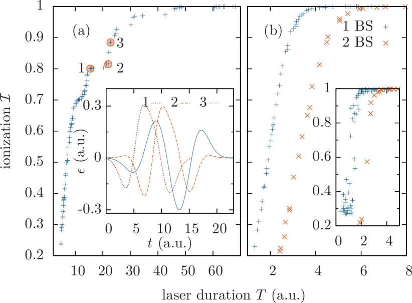
Figure 1: (Color online) (a) Ionization of the system with one bound electron as a function of laser duration for the optimal lasers with $E_{\text{L}}=2$ Ha. The inset shows the lasers amplitudes $\epsilon(t)$ for the marked points. (b) Ionization at $E_{\text{L}}=60$ Ha., for the system with only one bound state (blue), and with two bound states (red). The inset shows $\mathcal{I}$ as a function $T$ for the same lasers using a classical model.

Figure 1 shows the Pareto fronts for two sample laser energies: $E_{\text{L}}=2$ Ha (a) and $E_{\text{L}}=60$ Ha (b). For fixed laser fluence, the total ionization increases monotonically with the total duration of the laser. Also, as expected, more energetic lasers can ionize faster the electron.

In the left panel (a) the front is not smooth, exhibiting a series of steps. They are observable up to $E_{\text{L}}=10$ Ha. The inset proves how these steps are due to a qualitative change in the laser shapes, such as the addition of one half-cycle by which the lasers labeled 2 and 3 differ. Such abrupt changes in the ionization behaviour, due to subcycle dynamics, has also been observed experimentally Uiberacker et al. (2007) in the regime of nonadiabatic tunneling . The steps can be alternatively understood in terms of changes of the carrier envelope phase $\phi$, and this fact underlines the importance of this phase in this ionization regime, as lasers 2 and 3 have essentially the same duration $T\approx 23$ a.u. and the same frequency $\omega\approx 0.67$ Ha, differing only by $\phi$.

For higher laser energies, as in the case shown in the right panel (b), a complete ionization is obtained in one cycle, and the Pareto front becomes smoother. For $E_{\text{L}}=60$ Ha a simple classical model even suggests over-the-barrier ionization instead of nonadiabatic tunneling ionization: the laser deforms the atomic field $U_{\text{PT}}$, such that the electron density is spilled out. Using a simple classical model, we initialized a distribution of point-like, noninteracting classical particles according to the ground-state density of the potential given by Eq. (1). By following their trajectories in the combined potential $U_{\text{PT}}(x)-\epsilon(t)x$, we could determine if, and when, they cross this barrier. Despite its simplicity (most notably, the quantized bound states are missing), this model reproduces well the differences in ionization times for the two different $U_{\text{PT}}$ (with 1 BS and 2 BS): $\sim\!2$ a.u. (cf. the inset in Fig. 1b).

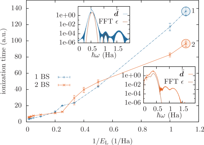
Figure 2: (Color online) Ionization time as a function of inverse laser energy. The insets show the dipole acceleration of the electron system, and the Fourier transform (FFT) of the laser at the marked points of the main panel (top inset for point 1, bottom inset for point 2).

The analysis of the Pareto fronts permits to define a total “ionization time” for each laser energy $E_{\text{L}}$ by intersecting the front at a given ionization probability. In the following we will take this threshold to be $\mathcal{I}(T)=0.98\pm 0.005$, i.e., the almost complete ionization of the electron. In Fig. 2 we report the dependence of these total ionization times on the inverse laser energy for the 1 BS system and the 2 BS system (the presence of the error bars is due to the use of an uncertainty of $\pm 0.005$ in the above definition). The range of $1/E_{\text{L}}$ covers all ionization regimes: the above mentioned over-the-barrier ionization, nonadiabatic tunneling and multiphoton ionization. Note that the average intensity of the lasers under consideration in SI units is between $3\times 10^{13}$ and $10^{17}$ W/cm². We prefer not to make use of cycle-averaged quantities, as the Keldysh parameter Keldysh (1964), to distinguish the regimes, due to the very short duration of the pulses.

At high laser energies (left part of the graph in Fig. 2), one full cycle is sufficient to ionize both the 1 BS and the 2 BS systems; the 1 BS system ionizes first. The situation is changed at around $1/E_{\text{L}}=0.25$ Ha^-1: at those energies, the second bound state of the 2 BS system serves as an intermediate state for the electron, before leaving the atom – the so-called shake-up-and-ionize mechanism Uiberacker et al. (2007). As a consequence, for the 2 BS system a single full cycle suffices to ionize the atom, while for the 1 BS system the shortest ionizing laser consists of three half-cycles. The situation is reversed between $1/E_{\text{L}}=0.4$ and 0.6 Ha^-1, but the shake-up-and-ionize mechanism produces an even faster ionization at the lowest energies (highest inverse $E_{\text{L}}$). In fact, at those energies, the process for the 2 BS system is better understood by considering it in the nonadiabatic tunneling regime, while for the 1 BS system the process is best understood in the multiphoton absorption regime.

The insets in Fig. 2 may help to understand this. They show the Fourier transform (in fact, the power spectrum) of the field and of the acceleration of the dipole moment, for the 1 BS system (top) and for the 2 BS system (bottom), for the circled points, tagged 1 and 2 respectively. According to the dipole acceleration $\ddot{\bm{d}}$, i.e. the optical absorption/emission of the electron system, the 1 BS system mainly absorbs at the ionization potential $0.5$ Ha, while the 2 BS system absorbs at lower energies, i.e. at the frequency of the bound-bound transition ($0.38$ Ha), and at the ionization energy from the excited-state ($0.12$ Ha). Consequently, at low laser energy, the electron is excited to the excited-state (shake-up), and subsequently tunnels out. This route is faster than single- or multiphoton absorption of the 1 BS system.

The upper inset also shows the power spectrum of the laser, for the 1 BS system. Indeed, the first two peaks ($0.5$ and $1.1$ Ha) of the power spectrum of the dipole acceleration are also present in the power spectrum of the laser. The third peak at $1.6$ Ha in the power spectrum of the dipole acceleration can then be interpreted as the absorption of two distinct photons of the former energies. In the lower inset, corresponding to the 2 BS system, one observes, apart from the excitation energies ($0.12$ Ha and $0.38$ Ha) in the Fourier transform of the laser and in the absorption/emission, two further peaks for $\ddot{\bm{d}}$ at $\sim\!0.84$ Ha, the $7$th harmonic of $0.12$ Ha, and at $\sim\!1.14$ Ha, the $3$rd harmonic of $0.38$. The generation of high harmonics is best understood in terms of tunneling, by making use of the three-step model Corkum (1993).

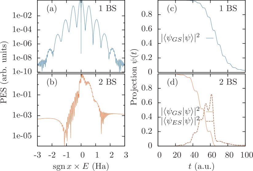
Figure 3: (Color online) Angle-resolved photoelectron spectra for the 1 BS system (a) and the 2 BS system (b), and projections of the evolving wavefunction for 1 BS (c) and 2 BS (d) at $1/E_{\text{L}}=1.1$ Ha.

Figure 3 further analyzes the ionization dynamics at $1/E_{\text{L}}=1.1$, the lowest laser energy, illustrating again how the two different ionization mechanisms of the two systems (with and without one bound excited state) produce different spectroscopic signatures. Panels (a) and (b) show the “angle-resolved” (in 1D: left-right) photoelectron spectrum of both systems. The spectrum of the 1 BS system exhibits equally distanced peaks with decreasing intensity. This spectrum shape is typical of above threshold ionization, where the electron absorbs more photons than necessary to overcome the ionization barrier. The symmetry is due to the fact that the ionization is considered to be “vertical”, i.e. independent of any preferred direction of the field. The spectrum of the system with 2 BS, instead, differs in two points: first, it is not symmetric with respect to left and right from the atomic position, second, it does not have distinct, equally distant peaks. Both properties are characteristics typical of nonadiabtaic tunneling Chelkowski and Bandrauk (2005).

Finally, Fig. 3 displays in panels (c) and (d) the projection of the propagated electron wavefunction onto bound field-free states. It once again helps to understand how the two ionizations proceed differently. The electron of the 2 BS system is first promoted to the excited state, leading to a peak in the projection of the wavefunction on it [Fig. 3(d)], and then tunnels out of the atomic potential.

IV Conclusions

We have analyzed the time it takes to photo-ionize a hydrogen-like model system, and how the variation of the shape of the laser pulse may be used to accelerate the process. For this purpose, we set-up a Pareto optimization scheme with the double objective of increasing ionization and reducing ionization time, and used a genetic-type algorithm (the differential evolution) to perform the optimizations. The search was performed on spaces of pulses carrying fixed energies per unit area, and we looked at different regimes by considering differents energies. The presence or absence of intermediate bound states was found to be relevant, since it may determine what is the fastest ionization channel. The shake-up-and-ionize mechanism may in fact lead to the fastest channel, depending on the energy carried by the laser pulse. The process may also have signatures of tunneling, or of multi-photon ionization. The possibility of designing pulse shapes that significantly accelerate ionization may be relevant to shed light into the problem of defining and measuring the times of these processes, and may be of use for the experimental design of atto-second resolution chronometers.