From Network Reliability to the Ising Model:
A Parallel Scheme for Estimating the Joint Density of States

Abstract

Network reliability is the probability that a dynamical system composed of discrete elements interacting on a network will be found in a configuration that satisfies a particular property. We introduce a new reliability property, Ising-feasibility, for which the network reliability is the Ising model’s partition function. As shown by Moore and Shannon, the network reliability can be separated into two factors: structural, solely determined by the network topology, and dynamical, determined by the underlying dynamics. In this case, the structural factor is known as the joint density of states. Using methods developed to approximate the structural factor for other reliability properties, we simulate the joint density of states, yielding an approximation for the partition function. Based on a detailed examination of why naïve Monte Carlo sampling gives a poor approximation, we introduce a novel parallel scheme for estimating the joint density of states using a Markov chain Monte Carlo method with a spin-exchange random walk. This parallel scheme makes simulating the Ising model in the presence of an external field practical on small computer clusters for networks with arbitrary topology with $\sim 10^{6}$ energy levels and more than $10^{308}$ microstates.

I Introduction

The Ising model Lenz (1920); Ising (1925) of ferromagnetism in crystals has been the object of sustained scrutiny since its introduction nearly a century ago, due to the rich phenomenology it produces from simple dynamics McCoy and Maillard (2012); Taroni (2015). The Ising model has also had a far-reaching influence in domains ranging from protein folding Tanaka and Scheraga (1977) to social science Schelling (1971); Stauffer and Solomon (2007). Yet it has proven resistant to analytical solution, except in special cases such as 1 or 2-dimensional lattices with no external field. Indeed, solving the model in the general case is known to be NP-hard Barahona (1982); Unger and Moult (1993); Istrail (2000). Hence we largely depend on approximations or numerical simulations for understanding its properties. Unfortunately, the naïve Metropolis algorithm suffers from poor convergence at precisely the most interesting region of parameter space, the critical point Metropolis et al. (1953); Swendsen and Wang (1987). Wang and Landau Wang and Landau (2001a, b) proposed a more efficient algorithm that focuses on estimating the density of states. Once the density of states is known, the system’s partition function and related thermodynamic quantities can be computed without further simulation. The original sequential Wang-Landau method is not practical for large systems, because its convergence time increases rapidly with the number of energy states. The state-of-the-art replica-exchange framework Vogel et al. (2013, 2014) provides a parallel algorithm to estimate the univariate density of states $g\left(k\right)$. However, it is not clear how to apply this parallel scheme to estimate the joint density of states $g\left(k,v\right)$, necessary for computing physical quantities in the presence of an external field. Here we use insights from Moore-Shannon network reliability Moore and Shannon (1956a, b) to construct a new parallel scheme that bridges the gap between the Wang-Landau approach and the estimation of joint density of states $g\left(k,v\right)$. The result is an efficient estimation scheme for the partition function of the Ising model in the presence of an external field that performs well even on large, irregular networks.

The Ising model is defined on a graph $G\left(V,E\right)$ with vertex and edge sets $V$ and $E$, respectively, by the Hamiltonian

$$H=J\sum_{\left(i,j\right)\in E}\sigma_{i}\sigma_{j}+\mu B\sum_{i\in V}\sigma_{i},$$ (1)

where $\sigma_{i}\in\left\{-1,1\right\}$ represents the state of the vertex $i$. $J$ is the coupling strength between neighboring vertices and $B$ is the external field. The exact solution of the Ising model in one dimension does not exhibit any critical phenomena. In the study of the order-disorder transformation in alloys, Bragg and Williams Bragg and Williams (1934, 1935) used a mean-field approximation for the Hamiltonian in which each individual vertex interacts with the mean state of the entire system. This is known as the Bragg-Williams approximation or the zeroth approximation of the Ising model Pathria (1996). An analytic expression for the partition function of a two-dimensional Ising model in the absence of an external field was given by Onsager Onsager (1944) and later derived rigorously by C. N. Yang Yang (1952). In spite of great effort in the seven decades since, the exact solution of the 2D Ising model in the presence of an external field remains unknown.

A network’s reliability is the probability it “functions” – i.e., continues to have a certain structural property – even under random failures of its components. It was proposed in 1956 by Moore and Shannon Moore and Shannon (1956a, b) as a theoretical framework for analyzing the trade-off between reliability and redundancy in telephone relay networks. The desired structural property in that case, known as “two-terminal” reliability, is to have a communication path between a specified source node and specified target node. Since then, a wide variety of properties have been studied, for example: “all-terminal” reliability requires the entire graph to be connected; “attack-rate-$\alpha$” reliability requires the root-mean-square of component sizes is no less than $\alpha N$ Youssef et al. (2013). Network reliability can be expressed as a polynomial in parameters of the dynamical system whose coefficients encode the interaction network’s structure. A reliability polynomial is the partition function of a physical system Essam and Tsallis (1986); Welsh and Merino (2000); Beaudin et al. (2010), but it emphasizes the role of an interaction network’s structure rather than the form of the interactions.

Specifically, the reliability of an interaction network $G\left(V,E\right)$ is

$$R\left(x;r,G\right)\equiv\sum_{s\in\mathcal{S}}r\left(s\right)p_{s}\left(x\right),$$ (2)

where $\mathcal{S}$ is the set of all subgraphs of $G\left(V,E\right)$; $r\left(s\right)\in\left\{0,1\right\}$ is a binary function indicating whether the subgraph $s$ has the desired property, i.e. “two-terminal”; and $p_{s}\left(x\right)$ is the probability resulting in a modified interaction subgraph $s$. The probability of picking a subgraph $p_{s}\left(x\right)$ reflects random, independent edge failures in the network with a failure rate $\left(1-x\right)\in\left[0,1\right]$ Moore and Shannon (1956a). Hence, with $M\equiv\left|E\right|$, $p_{s}\left(x\right)=x^{k}\left(1-x\right)^{M-k}$ where $k$ is the number of edges in the subgraph $s$.

If we group all $2^{M}$ subgraphs into $M$ equivalence classes by the number of edges in the subgraphs, the reliability can be expressed as

$$R\left(x;r,G\right)=\sum_{k=1}^{M}R_{k}\left(r,G\right)x^{k}\left(1-x\right)^{M-k}$$ (3)

where $R_{k}$ is the number of subgraphs with $k$ edges that have the desired property. As shown in Section II, $R_{k}$ is equivalent to the density of states in the Ising model.

Evaluating $R_{k}$ exactly is known to be as difficult as $\#P-complete$. In practice, however, $R_{k}$ can be estimated by $R_{k}=P_{k}{M\choose k}$, where $P_{k}$ is the fraction of subgraphs with the desired property, which can be estimated via sampling.

In summary, the reliability of a graph $G\left(V,E\right)$ with respect to a certain binary criterion can be written as a polynomial:

$$R\left(x;r,G\right)=\sum_{k=1}^{M}P_{k}\left(r,G\right){M\choose k}x^{k}\left(1-x\right)^{M-k}$$ (4)

Each term in the reliability polynomial, Eq. (4), contains two independent factors: a structural factor $P_{k}$ and a dynamical factor $x^{k}\left(1-x\right)^{M-k}$. The reason for calling this factor “dynamical” will become apparent in Section III. The structural factor depends only on the topology of the graph $G$ and the reliability criterion $r$, whereas the dynamical factor only depends on the parameter $x$ – for given values of $P_{k}$, the reliability $R$ is a function of $x$ alone.

This separation of dynamical and structural factors suggests new, more efficient ways to simulate Ising models. In Section II, we will illustrate that the reliability $R\left(x\right)$ is equivalent to the partition function $Z\left(\beta\right)$ of the Ising model; and the “failure rate” $1-x$ actually corresponds to physical quantities such as the temperature, the external field and the coupling strength in the Ising model. In Section III, we use this perspective to show that the Bragg-Williams approximation is given by the first-order term in a principled approximation to the structural factor. In Section IV, we use this perspective to extend the Wang-Landau method into an efficient parallel scheme for estimating the joint density of states, which we demonstrate on a $32\times 32$ square lattice and a Cayley tree.

II Network Reliability and Partition Function

The Ising model assumes that the state of a site is binary, either “spin-down” ($\sigma_{i}=-1$) or “spin-up” ($\sigma_{i}=1$), and that each site interacts only with its nearest neighbors, with a coupling strength $J$. All sites are exposed to a uniform external field $B$. The collection of all the sites’ states is called a “microstate” of the system. The Hamiltonian for the Ising model on a graph $G\left(V,E\right)$ is shown in Eq. (1). The canonical partition function $Z\left(\beta,B,J\right)$ is given by the summation of $\exp\left(-\beta H_{s}\right)$ over all possible microstates $s$: $Z\left(\beta,B,J\right)=\sum_{s}e^{-\beta H_{s}}$, where $\beta=\left(k_{B}T\right)^{-1}$ is the inverse temperature. In the alternative expression of the reliability polynomial Eq. (4), the summation over all subgraphs is organized into equivalence classes by the number of edges in the subgraphs. Similarly, we can group all microstates into equivalence classes (energy levels) determined by the number of adjacent sites in opposite states (“discordant vertex pairs” or “edges”) and the number of spin-up sites. With $N\equiv\left|V\right|$, the partition function can be expressed as:

$$Z\left(\beta,B,J\right)=C\sum_{k=0}^{M}\sum_{v=0}^{N}g\left(k,v\right)e^{-2\beta\left(Jk+\mu Bv\right)}$$ (5)

where $C\equiv e^{\beta\left(JM+\mu BN\right)}$ and $g\left(k,v\right)$ is the number of microstates with $v$ spin-up vertices and $k$ discordant adjacent vertex pairs (edges). Note that in the absence of an external field ($B=0$), the sum over $v$ reduces to the univariate density of states $g\left(k\right)$. Eq. (5) is a useful form for deriving a “low-temperature” expansion Pathria (1996), in which only equivalence classes with small $k$ and $v$ contribute. In analogy with the reliability polynomial Eq. (4), each term in Eq. (5) can be factored into two separate parts: structural – the number of microstates $g\left(k,v\right)$ determined by the graph, and dynamical – the physical quantities $\beta$, $J$ and $B$– or thermal to be more precise in the Ising model context. Just as the structural factors $R_{k}(r,G)$ of the reliability $R\left(x;r,G\right)$ can be computed independently of $x$, Eq. 3, $g\left(k,v\right)$ can be computed independently of $\beta$, $B$ or $J$. Once we have $g\left(k,v\right)$, we can plug in any value of physical quantities and compute the thermodynamic functions without any further simulation. This is more efficient than the traditional Metropolis methods. This observation has also been made by Wang and Landau Wang and Landau (2001a, b). By introducing the transformation $x\left(B,\beta\right)\equiv\left(1+e^{2\beta\mu B}\right)^{-1}$ and $y\left(J,\beta\right)\equiv\left(1+e^{2\beta J}\right)^{-1}$, we can express the partition function $Z\left(\beta,B,J\right)$ as a bivariate reliability polynomial $R\left(x,y;r,G\right)$ using the transformation $\beta\mu B\equiv\frac{1}{2}\ln\frac{1-x}{x}$ and $\beta J\equiv\frac{1}{2}\ln\frac{1-y}{y}$ (Appendix A):

$$Z\left(\beta,B,J\right) \propto \sum_{v,k}g\left(k,v\right)x^{v}\left(1-x\right)^{N-v}y^{k}\left(1-y\right)^{M-k}$$

$$= R\left(x,y;r,G\right)$$

Note that the density of states $g\left(k,v\right)$ is equivalent to $R_{k}$, the number of subgraphs satisfying a binary criterion, Eq. 3. We call the corresponding reliability criterion $r$ Ising-feasibility: a subgraph $s$ is Ising-feasible if and only if it is possible to find an assignment of spins to all vertices such that every pair of discordant vertices connected by an edge in $G$ is also connected by an edge in $s$ and there is no edge between any other pair of vertices. Fig. 1a illustrates an Ising-feasible microstate on a 4-by-4 square lattice; Fig. 1b, an infeasible one. Thus the Ising model’s partition function is a bivariate reliability polynomial with the special Ising-feasibility criterion.

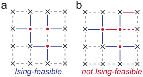
Figure 1: (a) An Ising-feasible configuration with three spin-up vertices (red dots) and eight discordant spin pairs or edges (solid line segments). (b) A configuration that is not Ising-feasible because of the inconsistent edges (red line segments). Independently choosing edges and spin-up vertices will rarely produce an Ising-feasible configuration, but any set of randomly chosen spin-up vertices uniquely determines a set of edges.

III $\delta-$Function Approximation

By definition, the structural factor $g\left(k,v\right)$ is independent of any of the physical variables, $\beta$, $J$, or $B$. Solving the Ising model numerically on any graph $G$ requires only estimating its joint density of states $g\left(k,v\right)$. Given the joint density of states, the partition function, and thus any thermodynamic quantities, can easily be evaluated for any particular values of $\beta$, $J$ and $B$. We use Monte Carlo sampling to estimate $g\left(k,v\right)$. Because sampling vertices and edges independently rarely produces an Ising-feasible configuration, we randomly assign $v$ vertices to be in the spin-up state and then measure the number of discordant node pairs (edges) $k$. We then estimate the conditional probability $p\left(k|v\right)$ by the frequency of producing $k$ edges given $v$ spin-up vertices. Because there are exactly ${N\choose v}$ ways to choose $v$ vertices, the joint density of states $g\left(k,v\right)$ can be expressed as $p\left(k|v\right){N\choose v}$. For example, on a 2D square lattice with periodic boundary conditions, when $v=1$ the only feasible microstates have $k=4$. Therefore, the number of microstates with 4 edges and 1 spin-up vertex is $g\left(4,1\right)=1\cdot{N\choose 1}=N$. Similarly, for $v=2$, $k=6$ when the two chosen vertices are neighbors and $k=8$ when they are not. Assuming $N\geq 4$, the corresponding conditional probabilities $p\left(k=6|v=2\right)=\frac{4}{N-1}$ and $p\left(k=8|v=2\right)=\frac{N-5}{N-1}$. The number of states $g\left(k=6,v=2\right)$ and $g\left(k=8,v=2\right)$ can be calculated accordingly by multiplying ${N\choose 2}$. These are the lowest order terms in the low temperature expansion. In general, $p\left(k|v\right)$ is very difficult to compute analytically.

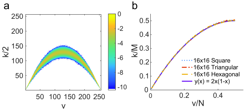
Figure 2: (a) Conditional state distribution of $p\left(k|v\right)$ sampled by a naïve Monte Carlo simulation on a 16-by-16 square lattice. The conditional probability is normalized separately for each value of $v$. The color reflects the value of $p\left(k|v\right)$ in logarithmic scale. As $p\left(k|v\right)$ is symmetric along $v=N/2$, the simulation is only done for $v\leq N/2$. (b) The peaks of $p\left(k|v\right)$ for various lattices have the same functional form: $y\left(x\right)=2x\left(1-x\right)$, where $x\equiv v/N$ and $y\equiv k/M$.

An example of $p\left(k|v\right)$ sampled using a naïve Monte Carlo method on a 16-by-16 square lattice is shown in Fig. 2a. Note that, because $p\left(k|v\right)$ is the conditional density function, it is normalized separately for each value of $v$ so that $\sum_{k}p\left(k|v\right)=1$. Also, for a 16-by-16 square lattice, $N=256$ and $M=512$, the maximum of $k$ can be as great as 512. This maximum is only achieved by a microstate in which spin-up and spin-down sites strictly alternate. There are only two such states out of ${256\choose 128}$ possible microstates with v=128. The naïve Monte Carlo method described above can hardly be expected to sample microstates as rare as this. Interestingly, as we explain in Section IV, these rare microstates can dominate the value of the joint density of states.

Empirically, the peaks of $p\left(k|v\right)$ lie on the curve $\frac{k}{M}=2\frac{v}{N}\left(1-\frac{v}{N}\right)$. This functional relationship seems independent of the system size $N$ or the coordination number (mean degree) $q\equiv 2M/N$ of the lattice, Fig. 2b. A simple argument suggests why this is the case. If the spin-up vertices are distributed uniformly across the lattice, the probability that the neighbor of a spin-up vertex is spin-down is $1-\frac{v}{N}$. For $v$ spin-up vertices, each with $q$ neighbors, the expected number of discordant pairs is thus $\frac{1}{2}qv(1-\frac{v}{N})$.

As the system size goes to infinity, $N\rightarrow\infty$, the conditional probability $p\left(k|v\right)$ becomes more sharply peaked at its center. We can approximate $p\left(k|v\right)$ as a Kronecker $\delta$-function $p\left(k|v\right)\simeq\delta\left(\frac{k}{M},2\frac{v}{N}\left(1-\frac{v}{N}\right)\right)$. Inserting the $\delta$-function approximation for $p\left(k|v\right)$ in our expression for the partition function, Eq. (5), yields:

$$Z\left(\zeta,\eta\right) = C\sum_{e,v}p\left(k|v\right){N\choose v}e^{-2\left(\zeta v+\eta k\right)}$$ (6)

$$\simeq C\sum_{e,v}\delta\left(k/M,y\left(v/N\right)\right){N\choose v}e^{-2\left(\zeta v+\eta k\right)}$$

$$\simeq C\sum_{v}{N\choose v}e^{-2N\left(\zeta\frac{v}{N}+\frac{1}{2}\eta qy\left(v/N\right)\right)}$$

where $\zeta\equiv\beta\mu B$, $\eta\equiv\beta J$ and $y\left(x\right)=2x\left(1-x\right)$. This produces the Bragg-Williams mean-field approximation Bragg and Williams (1934, 1935) , where the interaction term in the Hamiltonian $-J\sum_{\left(i,j\right)\in E}\sigma_{i}\sigma_{j}$ is approximated as $-J\left(\frac{1}{2}q\overline{\sigma}\right)\sum_{i}\sigma_{i}$, and $\overline{\sigma}=\frac{1}{N}\sum_{i}\sigma_{i}$ is the average spin of the system.

The Bragg-Williams mean-field approach – and hence Eq. 6 – incorrectly predicts that one-dimensional systems exhibit a critical point. According to Eq. 6, the partition function depends on the dimension of the system and the graph structure only through $q$, the coordination number, where $q=2$ for a 1D lattice, $q=4$ for a 2D square lattice and $q=6$ for a 2D triangular lattice. Moreover, its dependence on $q$ is only through the product $N\eta qy(x)$. If the external field is zero ($\zeta=0$), changing $q$ is equivalent to changing the system size $N$ or coupling strength $\eta$. In other words, a 2D square lattice with size $N$ behaves the same as a 1D lattice with size $2N$ in this approximation, which is physically incorrect. In Section IV we explore the causes of this failure and explain how to address it.

IV Estimating the Density of States

Although, for a particular $v$, it is reasonable to approximate $p\left(k|v\right)$ as a $\delta$-function, critical phenomena are determined by all $p\left(k|v\right)$ synergistically. The Ising model is hard to solve exactly because extremely rare events for one value of $v$ are as important as the most common events for another value. To demonstrate this, we first transform the conditional probability $p\left(k|v\right)$ to the number of states $g\left(k,v\right)=p\left(k|v\right){N\choose v}$. Since the binomial factor ${N\choose v}$ scales exponentially with $v$, it can dominate the ratio $g\left(k,v_{i}\right)/g\left(k,v_{j}\right)$. Ceteris paribus, this makes contributions to $Z$ from the tails of $p(k|v_{i})$ comparable to contributions from the peaks of $p\left(k|v_{j}\right)$. The joint density of states of a 5-by-5 2D lattice is shown in Fig. 3. Consider $g\left(16,5\right)$, the number of microstates with $k=16$ discordant neighbors when there are $v=5$ spins up. It corresponds to the peak of $p\left(k|5\right)$, and is roughly the same as $g(16,10)$, which is in the tail of $p\left(k|10\right)$. The naïve Monte Carlo method misses the tail of $p\left(k|v\right)$, and is thus inaccurate.

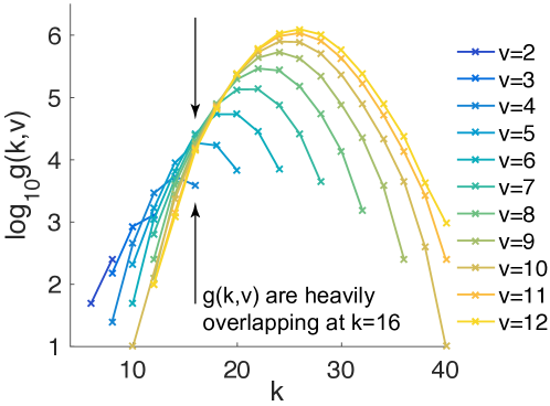
Figure 3: The exact joint density of states $g\left(k,v\right)$ computed via exhaustive enumeration on a 5-by-5 square lattice. Because a naïve Monte Carlo only samples points near the peak of each curve, and the tails of many curves are as important as the peaks of others, it severely underestimates the univariate density of states $g\left(k\right)\equiv\sum_{v}g\left(k,v\right)$ at $k=16$.

Despite the failure of the naïve Monte Carlo method, the strategy of dividing energy states into equivalence classes remains valuable. It separates the estimation of the joint density of states $g\left(k,v\right)$ into $N/2$ independent estimations of univariate distributions $p\left(k|v\right)$, thus enabling a novel parallel estimation scheme. And, each of $p\left(k|v\right)$ can be estimated using the improved Wang-Landau (WL) algorithmWang and Landau (2001a, b). The WL algorithm is a Markov-chain Monte Carlo algorithm to obtain the univariate density of states $g\left(k\right)$ for the Ising model.

The WL algorithm is very similar to the Metropolis-Hasting Metropolis et al. (1953); HASTINGS (1970) algorithm. However, instead of assuming the detailed balance condition, the WL algorithm pursues its so-called “flat” histogram by sculpting the $g\left(k\right)$ gradually during the simulation. Therefore, the running time of the WL algorithm largely depends on the number of energy states. As the number of states in $g\left(k,v\right)$ is proportional to $O\left(N^{2}\right)$, the square of the number of states in $g\left(k\right)$, the WL algorithm takes a tremendous amount of time to converge when computing the joint density of states Landau et al. (2004). Each step in the random walk in WL algorithm flips the spin of a random vertex, which inevitably changes both $v$ and $k$. Our modification of this algorithm is to constrain the random walk to maintain $v$ invariant. For each $v$-spin subspace, we assign an independent random walker. Therefore, the number of energy states is reduced to $O\left(N\right)$ for each walker. Specifically, instead of randomly flipping the spin of a vertex as is done in the WL random walk, each step of our random walk exchanges the locations of a spin-up vertex and spin-down vertex. The rest of the algorithm is as the same as the WL algorithm Wang and Landau (2001a), Appendix B.

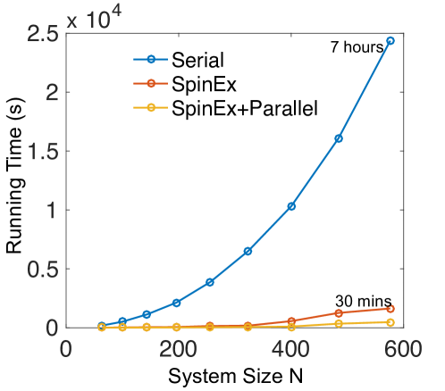
Figure 4: The running time for estimating the joint density of states $g\left(k,v\right)$ on 2D lattices of different sizes, from $N=8\times 8$ to $N=24\times 24$. The sequential Wang-Landau algorithm (blue) needs to cover $O\left(N^{2}\right)$ energy states, and become impractical for large systems. The spin-exchange WL algorithm (red) divides the energy states into $N/2$ energy slices, and the running time is bounded by the energy slice with the most number of states at $v=N/2$. This energy slice only contains $O\left(N\right)$ states. By dividing the energy slice into 6 equal-sized, 75% overlapping energy windows, the running time is reduced even further (yellow).

To demonstrate the efficiency of our algorithm, we compare the running time on 2D lattices of different sizes, from $N=8\times 8$ to $N=24\times 24$, Fig. 4. The number of energy states is proportional to $N^{2}$. The running time for the sequential WL algorithm (blue) grows exponentially as the number of energy states increases. It becomes impractical for large systems $N>10^{3}$. The spin-exchange method (red) splits the energy states into $N/2$ $v$-specific energy slices of different sizes. The overall running time is bounded by that of the slice for which $v=N/2$, which contains the most energy states. As the number of energy states in each slice is $O\left(N\right)$, the spin-exchange method is much faster than the sequential WL algorithm. Since each energy slice essentially is a univariate density, we can reduce the computation time even further by dividing an energy slice into multiple overlapping energy windows. We tested using six $75\%$ overlapping energy windows (yellow). The running time test simply assumes independent random walkers in each window. One can choose more sophisticated methods, such as the replica-exchange scheme Vogel et al. (2013, 2014).

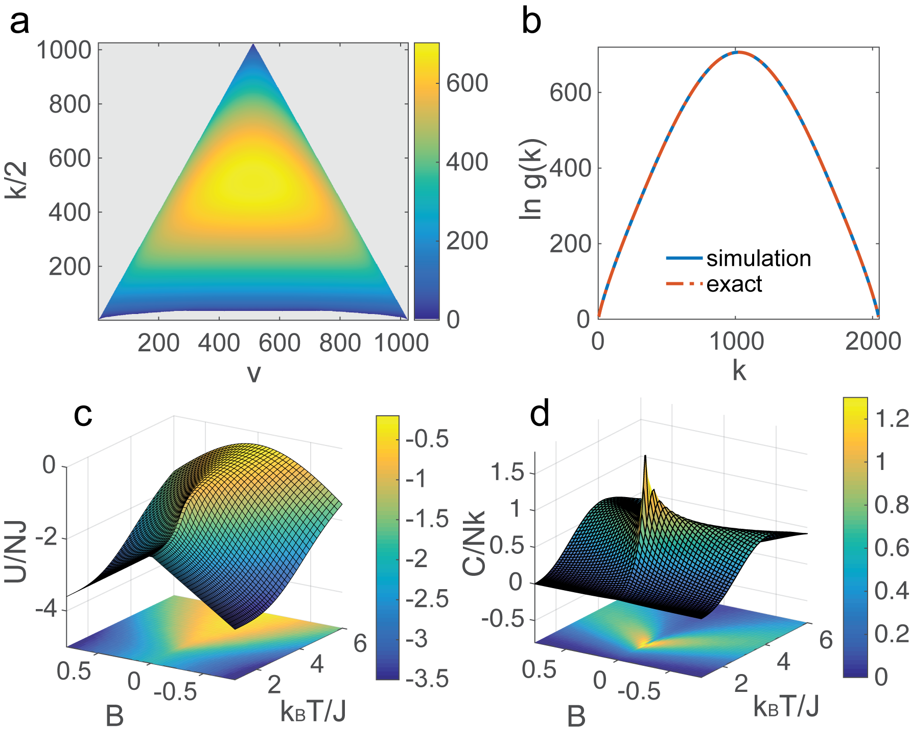
Figure 5: (a) The joint density of states $g\left(k,v\right)$ of a 32-by-32 square lattice. (b) The univariate density of states $g\left(k\right)\equiv\sum_{v}g\left(k,v\right)$ estimated using a spin-exchange MCMC algorithm, compared with the exact analytical result. (c) The internal energy $U=-\partial\ln Z/\partial\beta$, and (d) the heat capacity $C=\partial U/\partial T$ with coupling strength $J=0.5$.

We apply our algorithm on a 32-by-32 square lattice, with $\sim 0.5\times 10^{6}$ energy levels (equivalence classes) and more than $10^{308}$ microstates. Note that, for the same system, the univariate density of states $g\left(k\right)$ only has $\sim 10^{3}$ energy levels . Fig. 5a shows estimates for the joint density of states. The simulation is performed using 300 cores within two days. To verify this result, we compare its projection onto the univariate density of state $g\left(k\right)\equiv\sum_{v}g\left(k,v\right)$ with the known analytical result Beale (1996). As shown in Fig. 5b, the agreement is very good. Given the joint density of states, we can easily find the partition function $Z\left(\beta,B,J\right)$ using Eq. (5). Then, without additional simulations, any thermodynamic functions can be obtained directly from the partition function, such as the internal energy $U=-\partial\ln Z/\partial\beta$ and the heat capacity $C=\partial U/\partial T$. Fig. 5c and d show the internal energy $U$ and heat capacity $C$ as a function of inverse temperature $\beta$ and external field $B$ (assuming the magnetic susceptibility $\mu=1$) at $J=0.5$. The heat capacity curve presents the correct critical point of $k_{B}T/J=2.27$ at $B=0$. As the heat capacity is known to be very sensitive to the density of states, in Fig. 7a Appendix C, we show that the heat capacity at $B=0$ from our simulation agrees with the one from the analytic result.

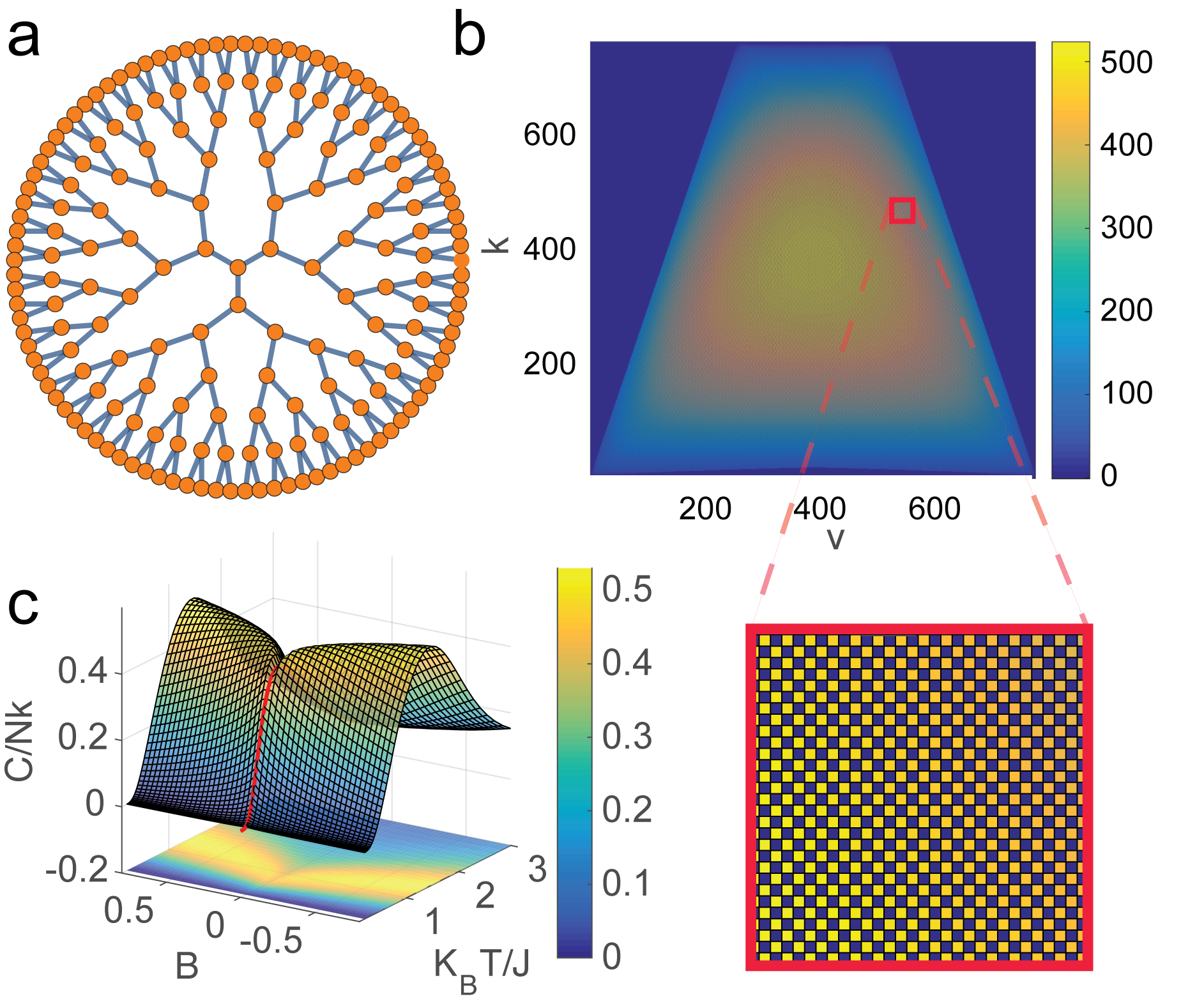
Figure 6: (a) A Cayley tree with degree $d=3$ and number of shells $r=6$. (b) The joint density of states $g\left(k,v\right)$ of the Cayley tree with $d=3$ and $r=8$ ($N=765$). As $d=3$, there are many inaccessible states. (c) The heat capacity of the Ising model on the Cayley tree. The red curve is from the exact solution at $B=0$.

We also apply our algorithm on Cayley trees (a finite-size analogue to Bethe lattices), where the exact result of the Ising model for $B=0$ is known Baxter (1982); Eggarter (1974). A Cayley tree has a central vertex and every vertex (except leaves) has $d$ neighbors, Fig. 6a. It is defined by two parameters, the degree $d$ and the number of shells $r$. There are $d\left(d-1\right)^{\left(j-1\right)}$ vertices at $j$-th shell and $d\left[\left(d-1\right)^{r}-1\right]/\left(d-2\right)$ vertices in total. So the ratio of the number of leaves to the system size tends to $\left(d-2\right)/\left(d-1\right)$. The dimensionality $\lim_{n\rightarrow\infty}\left(\ln c_{n}\right)/\ln n\rightarrow\infty$, where $c_{n}$ is the number of vertices within $n$ shells. All these characteristics make Cayley trees very different from a regular lattice and very interesting to study. The simulation on a Cayley tree with $d=3$ and $r=8$ ($N=765$) yields the joint density of states as shown in Fig. 6b. As $d=3$ in this particular Cayley tree, there are inaccessible states (“holes”) in the $g\left(k,v\right)$. The heat capacity is shown in Fig. 6c and a comparison with the analytic result at $B=0$ is shown in Fig. 7b in Appendix C. Due to the difference in topologies, the heat capacity of the Ising model on the Cayley tree is very different from that on the 2D square lattice.

The spin-exchange WL algorithm proposed above provides a unique and efficient parallel scheme for computing the joint density of states of Ising models in the presence of an external field. Essentially, this parallel scheme splits the joint density of states $g\left(k,v\right)$ into $N/2$ conditional densities $p\left(k|v\right)$.

V Conclusion

Network reliability is a general framework for understanding the interplay of network topology and network dynamics. Here we have used network reliability to study a prototypical network dynamical system – the Ising model. This framework can be adapted to other network dynamics as well, by defining a suitable feasibility criterion for microstates.

The network reliability perspective separates effects of network structure from dynamics in the system’s partition function. Based on this separation, we introduced a $\delta$-function approximation for the density of states, which leads to the Bragg-Williams approximation for the internal energy. We also showed why a naïve Monte Carlo method is not accurate enough for estimating the joint density of states. Finally, we introduced a novel parallel scheme using a spin-exchange MCMC algorithm for estimating the joint density of states. The scheme requires no inter-processor communication and can take advantage of the replica-exchange parallel framework. We applied our method to a periodic 32-by-32 square lattice estimating its internal energy and heat capacity as a function of both temperature and external magnetic field.

This work will make simulations of Ising-like dynamics on large, complex networks feasible and efficient, and opens the door to studying the Ising model in the presence of an external field. An efficient algorithm makes it possible to study the effects of network structure in systems that are too irregular to admit closed-form solutions. Furthermore, as is suggested by Fig. 5d, the nature of the phase transition depends on the external field strength. Our approach enables studies of such phenomena in large systems for the first time.

Appendix A

Here we show that the Ising model’s partition function, Eq. (5), can be expressed as the network reliability Eq. (4) under the transformation $x\left(\zeta\right)\equiv\left(1+e^{2\zeta}\right)^{-1}$ and $y\left(\eta\right)\equiv\left(1+e^{2\eta}\right)^{-1}$, where $\zeta\equiv\beta\mu B$ and $\eta\equiv\beta J$. The inverse transformations are $\zeta\equiv\frac{1}{2}\ln\frac{1-x}{x}$ and $\eta\equiv\frac{1}{2}\ln\frac{1-y}{y}$. Plugging $\zeta$ and $\eta$ into the partition function Eq. (5) gives:

$$Z\left(\zeta,\eta\right) = e^{\eta M+\zeta N}\sum_{k=0}^{M}\sum_{v=0}^{N}g\left(v,k\right)e^{-2\eta k-2\zeta v}$$

$$= e^{\left(\frac{1}{2}M\ln\frac{1-y}{y}+\frac{1}{2}N\ln\frac{1-x}{x}\right)}\sum_{k=0}^{M}\sum_{v=0}^{N}g\left(v,k\right)e^{-k\ln\frac{1-y}{y}-v\ln\frac{1-x}{x}}$$

$$= \left(\frac{1-y}{y}\right)^{\frac{M}{2}}\left(\frac{1-x}{x}\right)^{\frac{N}{2}}\sum_{k=0}^{M}\sum_{v=0}^{N}g\left(v,k\right)\left(\frac{y}{1-y}\right)^{k}\left(\frac{x}{1-x}\right)^{v}$$

$$= \left(y\left(1-y\right)\right)^{-\frac{M}{2}}\left(x\left(1-x\right)\right)^{-\frac{N}{2}}\sum_{k=0}^{M}\sum_{v=0}^{N}g\left(v,k\right)y^{k}\left(1-y\right)^{M-k}x^{v}\left(1-x\right)^{N-v}$$

$$= \left(y\left(1-y\right)\right)^{-\frac{M}{2}}\left(x\left(1-x\right)\right)^{-\frac{N}{2}}R\left(v,k;r,G\right)$$

Appendix B

The spin-exchange WL algorithm starts with a choice of $v\in[2,N/2]$, a prior unknown $p\left(k|v\right)$ and a histogram $H\left(k|v\right)$. At each step of the random walk, the system selects a new state $k^{\prime}$ with probability $P=\min\left(1,p\left(k|v\right)/p\left(k^{\prime}|v\right)\right)$. The $p\left(k^{*}|v\right)$ and $H\left(k^{*}|v\right)$ of the accepted state $k^{*}$ ($k^{*}=k$ or $k^{\prime}$) will be updated: $p\left(k^{*}|v\right)\leftarrow f\cdot p\left(k^{*}|v\right)$ and $H\left(k|v\right)\leftarrow H\left(k|v\right)+1$, where $f$ is a modification factor. Once the histogram $H\left(k|v\right)\geq 1/\sqrt{f},\ \forall k$ is sufficiently “flat”Zhou and Bhatt (2005), it is reset to zero $H\left(\cdot|v\right)\leftarrow 0$, and the modification factor is downscaled $f\leftarrow\sqrt{f}$. The simulation stops when the modification factor $f$ is very close to 1, e.g. $\exp\left(10^{-6}\right)$.

Appendix C

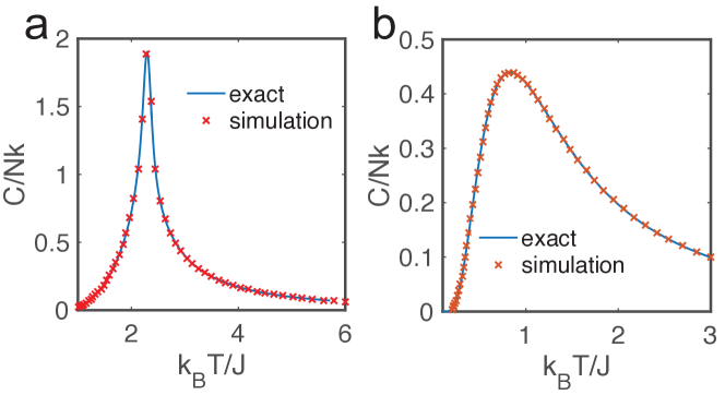
Figure 7: Compare the heat capacity with the known results at $B=0$ (without external field). (a) On a $32\times 32$ 2D square lattice. The exact solution is calculated from the exact density of states $g\left(k\right)$ from P.D. Beale Beale (1996). (b) On a $d=3$ and $r=6$ Cayley tree. The exact solution is computed as $C/k=-\beta^{2}d^{2}\ln Z/d\beta^{2}$, where $\ln Z$ is given by Eggarter (1974).

References

- Lenz (1920) W. Lenz, Physikalische Zeitschrift 21, 613 (1920).
- Ising (1925) E. Ising, Physikalische Zeitschrift 31, 253 (1925).
- McCoy and Maillard (2012) B. M. McCoy and J.-M. Maillard, Progress of Theoretical Physics 127, 791 (2012).
- Taroni (2015) A. Taroni, Nat Phys 11, 997 (2015).
- Tanaka and Scheraga (1977) S. Tanaka and H. A. Scheraga, Proceedings of the National Academy of Sciences 74, 1320 (1977).
- Schelling (1971) T. C. Schelling, The Journal of Mathematical Sociology, The Journal of Mathematical Sociology 1, 143 (1971).
- Stauffer and Solomon (2007) D. Stauffer and S. Solomon, The European Physical Journal B 57, 473 (2007).
- Barahona (1982) F. Barahona, Journal of Physics A: Mathematical and General 15, 3241 (1982).
- Unger and Moult (1993) R. Unger and J. Moult, Bulletin of Mathematical Biology 55, 1183 (1993).
- Istrail (2000) S. Istrail, in Proceedings of the Thirty-second Annual ACM Symposium on Theory of Computing, STOC ’00 (ACM, New York, NY, USA, 2000) pp. 87–96.
- Metropolis et al. (1953) N. Metropolis, A. W. Rosenbluth, M. N. Rosenbluth, A. H. Teller, and E. Teller, The Journal of Chemical Physics 21, 1087 (1953).
- Swendsen and Wang (1987) R. H. Swendsen and J.-S. Wang, Phys. Rev. Lett. 58, 86 (1987).
- Wang and Landau (2001a) F. Wang and D. P. Landau, Phys. Rev. Lett. 86, 2050 (2001a).
- Wang and Landau (2001b) F. Wang and D. P. Landau, Phys. Rev. E 64, 056101 (2001b).
- Vogel et al. (2013) T. Vogel, Y. W. Li, T. Wüst, and D. P. Landau, Phys. Rev. Lett. 110, 210603 (2013).
- Vogel et al. (2014) T. Vogel, Y. W. Li, T. Wüst, and D. P. Landau, Phys. Rev. E 90, 023302 (2014).
- Moore and Shannon (1956a) E. Moore and C. Shannon, Journal of the Franklin Institute 262, 191 (1956a).
- Moore and Shannon (1956b) E. Moore and C. Shannon, Journal of the Franklin Institute 262, 281 (1956b).
- Bragg and Williams (1934) W. L. Bragg and E. J. Williams, Proceedings of the Royal Society of London A: Mathematical, Physical and Engineering Sciences 145, 699 (1934).
- Bragg and Williams (1935) W. L. Bragg and E. J. Williams, Proceedings of the Royal Society of London A: Mathematical, Physical and Engineering Sciences 151, 540 (1935).
- Pathria (1996) R. K. Pathria, Statistical Mechanics, Second Edition (Butterworth-Heinemann, 1996).
- Onsager (1944) L. Onsager, Phys. Rev. 65, 117 (1944).
- Yang (1952) C. N. Yang, Phys. Rev. 85, 808 (1952).
- Youssef et al. (2013) M. Youssef, Y. Khorramzadeh, and S. Eubank, Phys. Rev. E 88, 052810 (2013).
- Essam and Tsallis (1986) J. W. Essam and C. Tsallis, Journal of Physics A: Mathematical and General 19, 409 (1986).
- Welsh and Merino (2000) D. J. Welsh and C. Merino, Journal of Mathematical Physics 41, 1127 (2000).
- Beaudin et al. (2010) L. Beaudin, J. Ellis-Monaghan, G. Pangborn, and R. Shrock, Discrete Mathematics 310, 2037 (2010).
- HASTINGS (1970) W. K. HASTINGS, Biometrika 57, 97 (1970).
- Landau et al. (2004) D. P. Landau, S.-H. Tsai, and M. Exler, American Journal of Physics 72, 1294 (2004).
- Beale (1996) P. D. Beale, Phys. Rev. Lett. 76, 78 (1996).
- Baxter (1982) R. J. Baxter, Exactly solved models in statistical mechanics (Academic Press, 1982).
- Eggarter (1974) T. P. Eggarter, Phys. Rev. B 9, 2989 (1974).
- Zhou and Bhatt (2005) C. Zhou and R. N. Bhatt, Phys. Rev. E 72, 025701 (2005).